Gated Deeper Models are Effective Factor Learners
Abstract
Precisely forecasting the excess returns of an asset (e.g., Tesla stock) is beneficial to all investors. However, the unpredictability of market dynamics, influenced by human behaviors, makes this a challenging task. In prior research, researcher have manually crafted among of factors as signals to guide their investing process. In contrast, this paper view this problem in a different perspective that we align deep learning model to combine those human designed factors to predict the trend of excess returns. To this end, we present a 5-layer deep neural network that generates more meaningful factors in a 2048-dimensional space. Modern network design techniques are utilized to enhance robustness training and reduce overfitting. Additionally, we propose a gated network that dynamically filters out noise-learned features, resulting in improved performance. We evaluate our model over 2,000 stocks from the China market with their recent three years records. The experimental results show that the proposed gated activation layer and the deep neural network could effectively overcome the problem. Specifically, the proposed gated activation layer and deep neural network contribute to the superior performance of our model. In summary, the proposed model exhibits promising results and could potentially benefit investors seeking to optimize their investment strategies.
Keywords: Deep neural network; Gated activation layer; Excess returns
1 Introduction
Deep learning has emerged as a powerful technique in the interdisciplinary field of computational finance, particularly in the area of quantitative factor mining. The promising capability of deep learning methods in analyzing large, complex, and high-dimensional datasets has enabled researchers to develop more accurate models for predicting financial market movements. Traditional methods, such as linear regression and time series analysis, have shown limitations in handling the intricate nature of financial data, thus leading to an increased interest in applying advanced deep learning techniques for better predictions and decision-making.
In the past decade, a rapid growing research have been conducted to explore adopting deep learning methods in computational finance. For instance, (Xiong et al., 2015) employed an LSTM neural network to model the volatility of the S&P 500 index, incorporating Google domestic trends as proxies for public sentiment and macroeconomic factors. Their work showed applicability to speech time series data. Singh and Srivastava (2017) applied deep learning to stock prediction, evaluating its performance on Google stock price multimedia data sourced from NASDAQ. Gao et al. (2016) aimed to achieve high precision in stock market forecasting using deep learning methods, with a focus on Stock Technical Indicators (STIs) Agrawal et al. (2019). Lin et al. (2018) utilized an LSTM model to learn and forecast the stock market valuation indicator, price-earnings ratio (P/E ratio). Jiang (2021) provided a comprehensive review of recent progress in deep learning applications for stock market prediction. Researchers have been exploring various machine learning tools with the objective of building effective prediction models.
In this paper, our goal is to construct a novel neural network model that combines Feedforward networks and Gated activation layers to predict whether a stock’s future excess returns will be positive. Excess returns refer to the portion of a stock’s performance that exceeds the market benchmark. Our proposed model addresses some limitations of previous models by incorporating advanced deep learning techniques and leveraging cutting-edge computational resources. The significance of this model lies in its potential to improve investment decision-making, enhance portfolio optimization, and facilitate risk management, ultimately contributing to the advancement of the computational finance industry.
2 Preliminary
In this paper, we mainly focus on identify the effective Alphas that can determine whether the future excess returns of stocks will be positive, that is, whether the future price changes of stocks can outperform the market average. Comparing with forecasting the future returns of stocks, forecasting the direction of excess returns of stocks is more straightforward and could eliminate noise to faithfully evaluate the quality of factors.
2.1 Quantitative trading alphas
The concept of Alpha () was originally derived from the capital asset pricing model (CAPM) Sharpe (1964), where it considers a linear relationship between the return of the asset and that of the market portfolio at each time step :
| (1) |
where is the return of the asset , is the risk-free rate, refers to the expected return of the market, and is the error term which can not be captured by this linear model. Then the excess return is defined as the left-hand side of the equation of CAPM:
| (2) |
According to the above formula, portfolio returns can be divided into two parts: return, which is the return compensation for bearing systematic (market) risk calculated by CAPM, and return, which is the difference in returns compared to the market benchmark and is not affected by market movements. Therefore, is considered a better measure of a stock’s true value and is most commonly used in multi-factor stock selection models. Here, the return made by the alphas and system are respectively defined as:
| (3) |
and
| (4) |
In this study, we focusing on constructing better factors to achieve higher alpha return .
2.2 Multi-factor stock selection models
A multi-factor stock selection model is a quantitative investment strategy that uses a combination of different financial factors to predict the future performance of stocks. Alpha factor is a critical component of multi-factor models, representing the excess return generated by a stock beyond its exposure to market risk. These alpha factors can be derived from a range of metrics, including fundamental indicators like earnings, revenue, and book value, as well as technical indicators like moving averages and momentum.
In this study, we aim to generate more factors that could effectively capture excess return of stocks for each stock and time step . To achieve this goal, we first introduce 101-Alpha factors Kakushadze (2015), which are dedicated designed by combining most popular price-volume-based signals (e.g., close-to-close returns, open price, close price, high price, low price, volume and vwap) with some financial formulations. The detail definitions of each factor in 101-Alpha is presented in the original article.
3 Method
3.1 Architecture
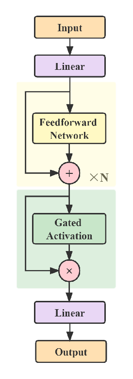
In this section, we present of our design for predicting the trend of future excess return of assets by aligning Alpha 101 factors. The model is primarily composes of two main modules, namely the Feedforward Networks and the Gated Activation Layer, where the former one is responsible to generating more meaningful in a higher dimensional space, while the later one dynamically select the new generated features. We also introduce batch normalization, skip connections, and dropout strategies into our model design to alleviate the degradation and overfitting problems for a robust training process. Figure 1 shows the overall architecture of our proposed model.
3.2 Feedforward Network
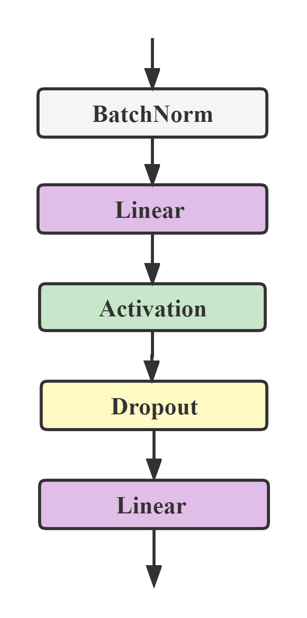
The naive Feedforward Network module includes two linear transformation layers and one non-linear (activation) layer . Specifically, we first use the first linear layer transform the input embedding into a ()-dimensional representation , then an activation layer is applied to operate the embedding . Here, the activation function is . Finally, the second linear layer is applied to map the high dimensional representation back into the original space . We expect the linear layers could learn an appropriate mapping between the input and output dimensions, thus enabling the embedding layers to capture and represent the underlying patterns and relationships within the input data.
Generally, stacking feedforward modules could increase the number of model capacity, enabling it to learn more complex feature representations and improve its performance. However, in some cases, adding more layers to a neural network may cause its performance to degrade, resulting in decreased accuracy as the depth of the network increases. This phenomenon is commonly referred to as the degradation problem, where the increased depth of the network causes the gradients to become smaller and prevents the model from properly learning and updating its weights. In this paper, we address this problem mainly by using batch normalization and residual connection. The residual connection is applied over each Feedforward module. That is, the output of each layer is , where denotes a Feedforward layer. To facilitate these residual connections, all embedding layers produce outputs of dimension . Additionally, batch normalization is introduced at the beginning of each feedforward module so that the strong dependency between two layers are decomposed. Finally, we adopt the dropout strategy over the outputs of the activation layer to encourage the second linear layer to learn more diverse and robust patterns from the high dimensional space. The strucuture of our feedforward network is presented in Figure 2(a).
Batch Normalization (BN).
The basic idea behind batch normalization is to normalize the input data for each mini-batch at each layer of the neural network, such that the mean is close to 0 and the variance is close to 1. The BN layer first determines the mean and the variance of the activation values across the batch:
| (5) |
Then the activation vector is normalized so that each neuron’s output follows a standard normal distribution across the mini-batch. The constant epsilon is used for numerical stability purposes:
| (6) |
Finally, the layer’s output is calculated by applying a linear transformation with two trainable parameters: and :
| (7) |
where is used to adjust the standard deviation and is used to adjust the center of the distribution.

Residual Connection.
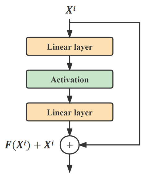
If we represent the formally underlying relationship between the input () and output () as for each neuron , we can train stacked nonlinear layers to fit an alternative mapping of . This allows us to transform the original mapping into . The rationale behind this approach is that it is generally easier to optimize the residual mapping than the original, as it involves fitting a smaller and simpler function Bishop (1995, 1999); Monti et al. (2018).
When the dimensions of and are unequal, we will perform a linear projection by the shortcut connections to match the dimensions:
| (8) |
where and are the input and output vectors of the layers; its the residual mapping to be learned and is a linear projection.
Based on the FeedForward network, we insert shortcut connections which turn the network into its counterpart residual version and presented in Figure 4. Through the linear projection in the above network, the dimensions of the outputs of layer 1 and layer 2 are the same and the identity shortcuts can be directly used.
Dropout.
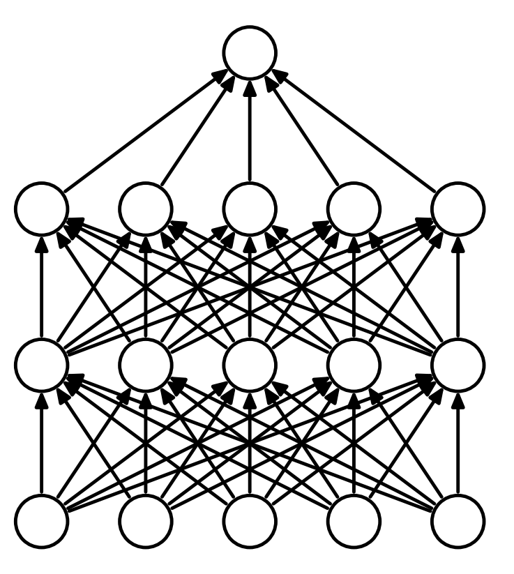
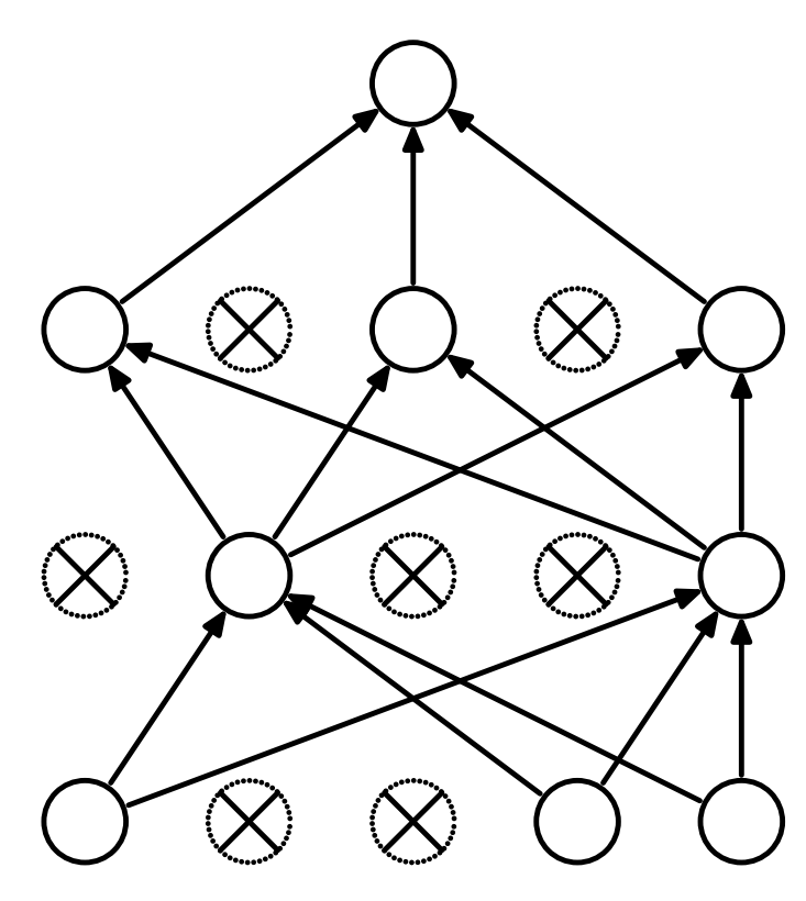
Dropout is a kind of computationally cheap and remarkably effective regularization method for reducing the overfitting problem and improving the generalization error in deep neural networks. It randomly sets a fraction of the activations in the neural network to zero during training, which forces the network to learn more robust features and reduces its reliance on any one activation.Srivastava et al. (2014)
3.3 Gated Activation Layer
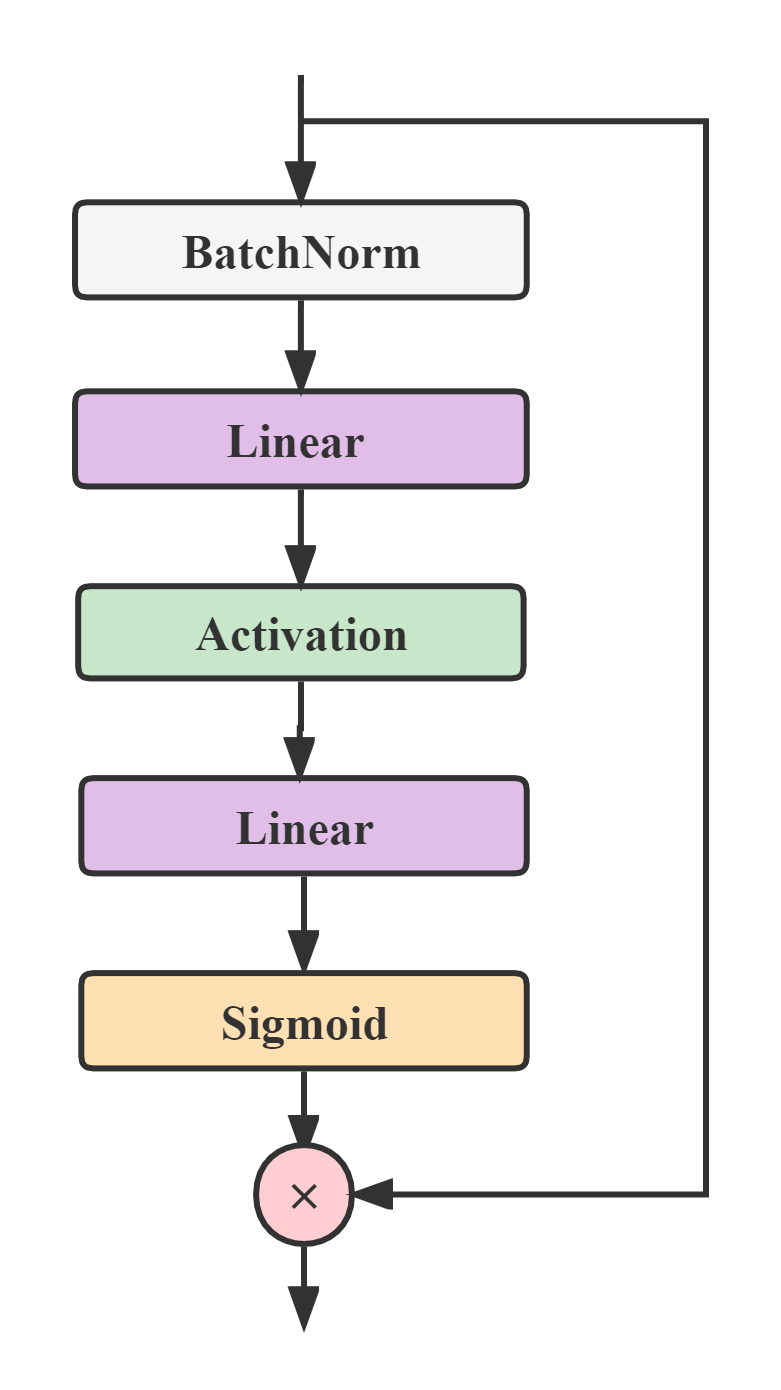
An essential aspect of constructing the Gated Activation Layer is its ability to perform denoising, which facilitates faster and more accurate model inference and improves the model’s robustness. As is shown in Figure 2(b), the Gated Activation Layer employs two linear transformations in a manner opposite to the Feedforward approach. The first linear transformation compresses the -dimensional data to dimensions, and the second one rescales it back to dimensions. After these transformations, we use the sigmoid function to extract effective factors from the reconstructed dimensions, while the information of ineffective factors is compressed during the compression process. Finally, we multiply the sigmoid-filtered output on the original layer input to eliminate noise, resulting in a refined output.
4 Experiments
4.1 Datasets
The main source of our data includes Wind Information Inc.(WIND) and China Stock Market & Accounting Research Database (CSMAR). The period of our data is from January 1, 2020, through March 1, 2023. Considering that institutions, organizations and individuals in China mainly trade in A-share market, we only select China A-shares that trade on the Shanghai Stock Exchange (SSE) in this paper.
Specifically, the stock data we need including daily technical data like open (opening price), close (closing price), high (daily highest price), low (dailylowest price), returns (daily close-to-close returns), volume(daily trading volume), vwap (daily volume-weighted average price), cap (market cap) and other fundamental data like cap(market cap) and ind (a generic placeholder for a binary industry classification such as GICS, BICS, NAICS, SIC, etc., where level = sector, industry, subindustry, etc. Multiple IndClass in the same alpha need not correspond to the same industry classification).
4.2 Settings
(1) The initial fundamental and technical indicators of stocks are transformed into 101 Alphas based on the formulas provided in "101 Formulaic Alphas" Kakushadze (2015). These 101 alphas serve as the initial inputs for our model.
(2) Testing set refers to the data from the last 70 days, while the training set includes all data before that. Additionally, a validation set was created by randomly selecting 5% of the training dataset.
(3) The dimension of the model is 512. The multiplier is 4 and divisor k is 8.
(4) The dropout rate is 15%.
(5) The output of total model is a one-dimension value, which is transformed by the last linear transformation: . The output of 1 means the expected excess return of stocks is positive and 0 means negative.
4.3 Results
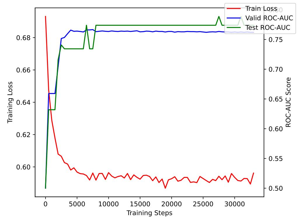
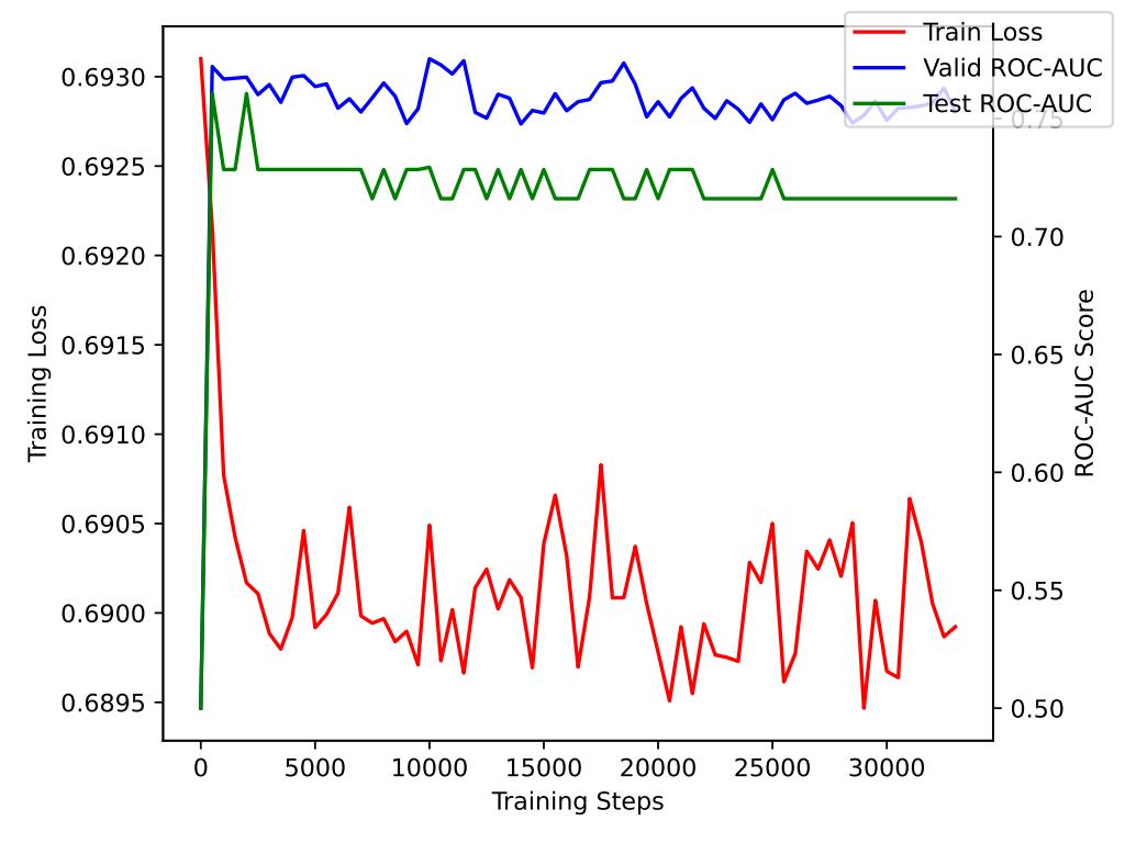
We benchmark our model against Linear regression, Simple MLP, Stack MLP and Deep MLP. Here Simple MLP is the Multilayer Perceptron with single hidden layer, Stack MLP is stacking the simple MLP modules over five times, and Deep MLP is a variation of the Stack MLP module empowered by batch normalization, skip connection, and the dropout strategies.
| Model | Valid | Test |
|---|---|---|
| Linear | 0.7681 | 0.6319 |
| Simple MLP | 0.7620 | 0.7343 |
| Stack MLP | 0.7531 | 0.7294 |
| Deep MLP | 0.7263 | 0.7887 |
| GatedDeep MLP | 0.7360 | 0.7962 |
Simply stacking layers could lead to degradation problem.
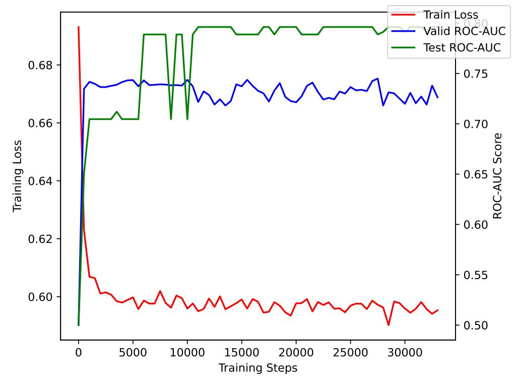
In Table1, the ROC-AUC score for the testing set of Stack MLP is 0.7294, which is lower than Simple MLP (0.7343). It shows that simply adding hidden layers is invalid for improving the model’s learning ability. The Stack MLP model’s AUC-ROC after 25000 steps did not improve significantly compared to its initial value.
Deeper models is beneficial in predicting.
Both Deep MLP and GatedDeep MLP perform better than Simple MLP and achieve high ROC-AUC scores for the testing set, which are 0.7887 and 0.7962 respectively.
Batch Normalization, Residual Connection and Dropout could enhance the model’s robustness.
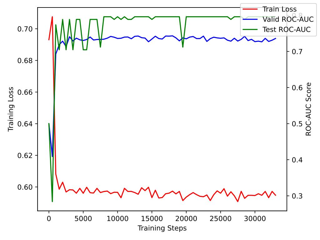
Deep MLP significantly outperforms Stack MLP. Besides higher ROC-AUC score, it is shown in Figure 6 that the training loss of Deep MLP obviously diverges and its ROC-AUC scores for the testing set quickly improves after 5000 steps.
The gated activation layer can improve the performance of model.
GatedDeepMLP outperforms the other three models on predicting the future excess return of stocks. Its ROC-AUC score (0.7962) is 1% higher than Deep MLP.
5 Future Works
The IC value is a metric that reflects the predictive power of a factor value on future returns. A larger absolute value of IC indicates a more effective factor. A negative IC indicates that a smaller factor value is better, while a positive IC indicates that a larger factor value is better.
Inspired by the concept of Information Coefficient (IC) which measures the correlation between a factor value and the cross-sectional next-period returns of a set of stocks, we have developed a new loss function:
| (9) | ||||
and
| (10) |
where:
-
is the value of factor for stock on day ;
-
is the excess return of stock on day ;
-
is the cosine similarity between the value of factor on day and the future excess return of stock on day ;
-
is the cosine similarity between the the value of factor on day and the value of factor on day . It is designed to address the issue of high correlation between the chosen factors. When factors are highly correlated, it can lead to problems such as multicollinearity and overfitting, which can affect the stability and reliability of the model.
Due to the high complexity of the proposed loss function, currently available computational resources are insufficient to run the experiments. However, future upgrades in computational power may enable the execution of this experiment.
6 Conclusion
In this study, we focus on the research problem about forecasting the trends of the asset’s excess returns. Specifically, we propose a deep neural network with gated activation layer to combine the manually designed factors. Our experimental results prove that the proposed Gated Deeper MLP model significantly outperform the Linear Regression and naive two-layers MLP model. We also prove the effective of the new deep learning strategies in enhancing the training robustness and alleviating the overfitting problem. We believe our findings from this paper could inspire further work in this challenging problem.
References
- Agrawal et al. (2019) Manish Agrawal, Asif Ullah Khan, and Piyush Kumar Shukla. 2019. Stock price prediction using technical indicators: a predictive model using optimal deep learning. Learning, 6(2):7.
- Bishop (1999) C. M. Bishop. 1999. Pattern Recognition and Feedforward Networks, page 629–631. MIT Press.
- Bishop (1995) Christopher M. Bishop. 1995. Neural Networks for Pattern Recognition. Oxford University Press, United Kingdom.
- Gao et al. (2016) Tingwei Gao, Xiu Li, Yueting Chai, and Youhua Tang. 2016. Deep learning with stock indicators and two-dimensional principal component analysis for closing price prediction system. In 2016 7th IEEE international conference on software engineering and service science (ICSESS), pages 166–169. IEEE.
- He et al. (2015) Kaiming He, X. Zhang, Shaoqing Ren, and Jian Sun. 2015. Deep residual learning for image recognition. 2016 IEEE Conference on Computer Vision and Pattern Recognition (CVPR), pages 770–778.
- Jiang (2021) Weiwei Jiang. 2021. Applications of deep learning in stock market prediction: recent progress. Expert Systems with Applications, 184:115537.
- Kakushadze (2015) Zura Kakushadze. 2015. 101 formulaic alphas. Risk Management & Analysis in Financial Institutions eJournal.
- Lin et al. (2018) Bo-Sheng Lin, Wei-Tao Chu, and Chuin-Mu Wang. 2018. Application of stock analysis using deep learning. In 2018 7th International Congress on Advanced Applied Informatics (IIAI-AAI), pages 612–617. IEEE.
- Monti et al. (2018) Ricardo Pio Monti, Sina Tootoonian, and Robin Cao. 2018. Avoiding degradation in deep feed-forward networks by phasing out skip-connections. In Artificial Neural Networks and Machine Learning–ICANN 2018: 27th International Conference on Artificial Neural Networks, Rhodes, Greece, October 4-7, 2018, Proceedings, Part III 27, pages 447–456. Springer.
- Sharpe (1964) William F Sharpe. 1964. Capital asset prices: A theory of market equilibrium under conditions of risk. The journal of finance, 19(3):425–442.
- Singh and Srivastava (2017) Ritika Singh and Shashi Srivastava. 2017. Stock prediction using deep learning. Multimedia Tools and Applications, 76:18569–18584.
- Srivastava et al. (2014) Nitish Srivastava, Geoffrey Hinton, Alex Krizhevsky, Ilya Sutskever, and Ruslan Salakhutdinov. 2014. Dropout: A simple way to prevent neural networks from overfitting. Journal of Machine Learning Research, 15:1929–1958.
- Xiong et al. (2015) Ruoxuan Xiong, Eric P Nichols, and Yuan Shen. 2015. Deep learning stock volatility with google domestic trends. arXiv preprint arXiv:1512.04916.