Towards Robust Probabilistic Modeling on SO(3)
via Rotation Laplace Distribution

Abstract

Estimating the 3DoF rotation from a single RGB image is an important yet challenging problem. As a popular approach, probabilistic rotation modeling additionally carries prediction uncertainty information, compared to single-prediction rotation regression. For modeling probabilistic distribution over $\mathrm{SO}(3)$, it is natural to use Gaussian-like Bingham distribution and matrix Fisher, however they are shown to be sensitive to outlier predictions, e.g. $180^{\circ}$ error and thus are unlikely to converge with optimal performance. In this paper, we draw inspiration from multivariate Laplace distribution and propose a novel rotation Laplace distribution on $\mathrm{SO}(3)$. Our rotation Laplace distribution is robust to the disturbance of outliers and enforces much gradient to the low-error region that it can improve. In addition, we show that our method also exhibits robustness to small noises and thus tolerates imperfect annotations. With this benefit, we demonstrate its advantages in semi-supervised rotation regression, where the pseudo labels are noisy. To further capture the multi-modal rotation solution space for symmetric objects, we extend our distribution to rotation Laplace mixture model and demonstrate its effectiveness. Our extensive experiments show that our proposed distribution and the mixture model achieve state-of-the-art performance in all the rotation regression experiments over both probabilistic and non-probabilistic baselines.

1 Introduction

Incorporating neural networks [1] to perform rotation regression is of great importance in the field of computer vision, computer graphics and robotics [2, 3, 4, 5, 6]. To close the gap between the $\mathrm{SO}(3)$ manifold and the Euclidean space where neural network outputs exist, one popular line of research discovers learning-friendly rotation representations including 6D continuous representation [7], 9D matrix representation with SVD orthogonalization [8], etc. Recently, Chen et al. [9] focuses on the gradient backpropagating process and replaces the vanilla auto differentiation with a $\mathrm{SO}(3)$ manifold-aware gradient layer, which sets the new state-of-the-art in rotation regression tasks.

Reasoning about the uncertainty information along with the predicted rotation is also attracting more and more attention, which enables many applications in aerospace [10], autonomous driving [11, 12] and localization [13, 14]. On this front, recent efforts have been developed to model the uncertainty of rotation regression via probabilistic modeling of rotation space. The most commonly used distributions are Bingham distribution [15] on $\mathcal{S}^{3}$ for unit quaternions and matrix Fisher distribution [16] on $\mathrm{SO}(3)$ for rotation matrices. These two distributions are equivalent to each other [17] and resemble the Gaussian distribution in Euclidean Space [15, 16]. While modeling noise using Gaussian-like distributions is well-motivated by the Central Limit Theorem, Gaussian distribution is well-known to be sensitive to outliers in the probabilistic regression models [18]. This is because Gaussian distribution penalizes deviations quadratically, so predictions with larger errors weigh much more heavily with the learning than low-error ones and thus potentially result in suboptimal convergence when a certain amount of outliers exhibit [19].

Unfortunately, in certain rotation regression tasks, we fairly often come across large prediction errors, e.g. $180^{\circ}$ error, due to either the (near) symmetry nature of the objects or severe occlusions [20]. In Fig. 1(left), using training on single image rotation regression as an example, we show the statistics of predictions after achieving convergence, assuming matrix Fisher distribution (as done in [21]). The blue histogram shows the population with different prediction errors and the red dots are the impacts of these predictions on learning, evaluated by computing the sum of their gradient magnitudes $\|\partial\mathcal{L}/\partial(\text{distribution param.})\|$ within each bin and then normalizing them across bins. It is clear that the 180^∘ outliers dominate the gradient as well as the network training though their population is tiny, while the vast majority of points with low error predictions are deprioritized. Arguably, at convergence, the gradient should focus more on refining the low errors rather than fixing the inevitable large errors (e.g. arose from symmetry). This motivates us to find a better probabilistic model for rotation.

As pointed out by [18], Laplace distribution, with heavy tails, is a better option for robust probabilistic modeling. Laplace distribution drops sharply around its mode and thus allocates most of its probability density to a small region around the mode; meanwhile, it also tolerates and assigns higher likelihoods to the outliers, compared to Gaussian distribution. Consequently, it encourages predictions near its mode to be even closer, thus fitting sparse data well, most of whose data points are close to their mean with the exception of several outliers[22, 23], which makes Laplace distribution to be favored in the context of deep learning[24].

In this work, we propose a novel Laplace-inspired distribution on $\mathrm{SO}(3)$ for rotation matrices, namely rotation Laplace distribution, for probabilistic rotation regression. We devise rotation Laplace distribution to be an approximation of multivariate Laplace distribution in the tangent space of its mode. As shown in the visualization in Fig. 1(right), our rotation Laplace distribution is robust to the disturbance of outliers, with most of its gradient contributed by the low-error region, and thus leads to a better convergence along with significantly higher accuracy. Moreover, our rotation Laplace distribution is simply parameterized by an unconstrained $3\times 3$ matrix and thus accommodates the Euclidean output of neural networks with ease. This network-friendly distribution requires neither complex functions to fulfill the constraints of parameterization nor any normalization process from Euclidean to rotation manifold which has been shown harmful for learning [9].For completeness of the derivations, we also propose the Laplace-inspired distribution on $\mathcal{S}^{3}$ for quaternions. We show that rotation Laplace distribution is equivalent to Quaternion Laplace distribution, similar to the equivalence of matrix Fisher distribution and Bingham distribution.

We extensively compare our rotation Laplace distributions to methods that parameterize distributions on $\mathrm{SO}(3)$ for pose estimation, and also non-probabilistic approaches including multiple rotation representations and recent $\mathrm{SO}(3)$-aware gradient layer [9]. On common benchmark datasets of rotation estimation from RGB images, we achieve a significant and consistent performance improvement over all baselines. For example, on ModelNet10-SO3 dataset, rotation Laplace distribution achieves relative improvement of around 35% on median error, and over 50% on 3 degree accuracy against the best competitor.

The superiority of rotation Laplace distribution are mainly benefited from the robustness to outliers. To gain a deeper understanding of this property, we provide more analysis from the aspect of training gradients, and further conduct experiments by manually injecting outliers into the perfectly labeled synthetic dataset. The results demonstrate that not only our model outperforms the baselines, but also better tolerate the outlier injections with significantly less performance degradation.

Additionally, due to the heavy-tail nature of our distribution, there is more probability density at the mode. One may concern that it will be sensitive to small noise perturbations of ground truths, since the wrong gradient around the mode can be large. To address this concern, we experiment with the perturbed data containing small noise injections and find that our method outperforms the baseline at all levels of perturbations and lead to comparable performance drop with the noise injections, illustrating its robustness to noise. Building upon these insights, we apply rotation Laplace distribution to the task of semi-supervised rotation regression where the pseudo labels are imperfect. Our method achieves new state-of-the-art in semi-supervised rotation regression tasks.

To better capture the multimodal rotation space, particularly for symmetric objects, we propose an extension of the rotation Laplace distribution in the form of a mixture model. Our rotation Laplace mixture model allows for the generation of multiple candidate predictions for one object, thereby improving its ability to capture the complete pose space for symmetric objects. We compare rotation Laplace mixture model with other methods that are capable capturing multimodal solutions and demonstrate the superior performance of our model.

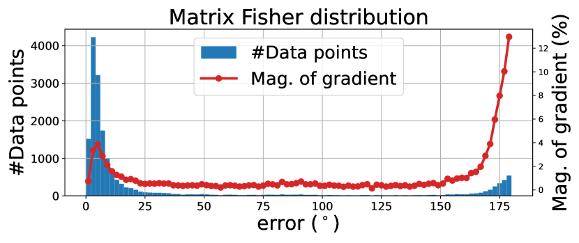
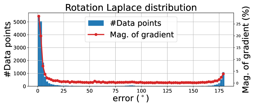
Figure 1: Visualization of the results of matrix Fisher distribution and rotation Laplace distribution after convergence. The horizontal axis is the geodesic distance between the prediction and the ground truth. The blue bins count the number of data points within corresponding errors (2^∘ each bin). The red dots illustrate the percentage of the sum of the gradient magnitude $\|\partial\mathcal{L}/\partial(\text{dist. param.})\|$ within each bin. The experiment is done on all categories of ModelNet10-SO3 dataset.

2 Related Work

2.1 Probabilistic regression

Nex and Weigend [25] first proposes to model the output of the neural network as a Gaussian distribution and learn the Gaussian parameters by the negative log-likelihood loss function, through which one obtains not only the target but also a measure of prediction uncertainty. More recently, Kendall and Gal [26] offers more understanding and analysis of the underlying uncertainties. Lakshminarayanan et al. [27] further improves the performance of uncertainty estimation by network ensembling and adversarial training. Makansi et al. [28] stabilizes the training with the winner-takes-all and iterative grouping strategies. Probabilistic regression for uncertainty prediction has been widely used in various applications, including optical flow estimation[29, 30], depth estimation [31, 32], weather forecasting [33], etc.

Among the literature of decades, the majority of probabilistic regression works model the network output by a Gaussian-like distribution, while Laplace distribution is less discovered. Li et al. [34] empirically finds that assuming a Laplace distribution in the process of maximum likelihood estimation yields better performance than a Gaussian distribution, in the field of 3D human pose estimation. Recent work [35] makes use of Laplace distribution to improve the robustness of maximum likelihood-based uncertainty estimation. Due to the heavy-tailed property of Laplace distribution, the outlier data produces comparatively less loss and have an insubstantial impact on training. Other than in Euclidean space, Mitianoudis et al. [22] develops Generalized Directional Laplacian distribution in $\mathcal{S}^{d}$ for the application of audio separation.

2.2 Probabilistic rotation regression

Several works focus on utilizing probability distributions on the rotation manifold for rotation uncertainty estimation. Prokudin et al. [36] uses the mixture of von Mises distributions [37] over Euler angles using Biternion networks. In [38] and [39], Bingham distribution over unit quaternion is used to jointly estimate a probability distribution over all axes. Mohlin et al. [21] leverages matrix Fisher distribution [16] on $\mathrm{SO}(3)$ over rotation matrices for deep rotation regression. Though both bear similar properties with Gaussian distribution in Euclidean space, matrix Fisher distribution benefits from the continuous rotation representation and unconstrained distribution parameters, which yields better performance [20]. Recently, Murphy et al. [20] introduces a non-parametric implicit pdf over $\mathrm{SO}(3)$, with the distribution properties modeled by the neural network parameters. Implicit-pdf especially does good for modeling rotations of symmetric objects.

2.3 Non-probabilistic rotation regression

The choice of rotation representation is one of the core issues concerning rotation regression. The commonly used representations include Euler angles [40, 41], unit quaternion [42, 43, 44, 45] and axis-angle [46, 47, 48], etc. However, Euler angles may suffer from gimbal lock, and unit quaternions doubly cover the group of $\mathrm{SO}(3)$, which leads to two disconnected local minima. Moreover, Zhou et al. [7] points out that all representations in the real Euclidean spaces of four or fewer dimensions are discontinuous and are not friendly for deep learning. To this end, the continuous 6D representation with Gram-Schmidt orthogonalization [7] and 9D representation with SVD orthogonalization [8] have been proposed, respectively. More recently, Chen et al. [9] investigates the gradient backpropagation in the backward pass and proposes a $\mathrm{SO}(3)$ manifold-aware gradient layer.

3 Notations and Definitions

3.1 Notations for Lie Algebra and Exponential & Logarithm Map

This paper follows the common notations for Lie algebra and exponential & logarithm map [49, 50, 51].

The three-dimensional special orthogonal group $\mathrm{SO}(3)$ is defined as

$$\mathrm{SO}(3)=\{\mathbf{R}\in\mathbb{R}^{3\times 3}|\mathbf{RR}^{T}=\mathbf{I},\det{(\mathbf{R})}=1\}.$$

The Lie algebra of $\mathrm{SO}(3)$, denoted by $\mathfrak{so}(3)$, is the tangent space of $\mathrm{SO}(3)$ at $\mathbf{I}$, given by

$$\mathfrak{so}(3)=\{\boldsymbol{\Phi}\in\mathbb{R}^{3\times 3}|\boldsymbol{\Phi}=-\boldsymbol{\Phi}^{T}\}.$$

$\mathfrak{so}(3)$ is identified with $(\mathbb{R}^{3},\times)$ by the hat $\wedge$ map and the vee $\vee$ map defined as

$$\mathfrak{so}(3)\ni\left[\begin{array}[]{ccc}0&-\phi_{z}&\phi_{y}\\ \phi_{z}&0&-\phi_{x}\\ -\phi_{y}&\phi_{x}&0\end{array}\right]\stackrel{{\scriptstyle\text{ vee }\vee}}{{\underset{\text{ hat }\wedge}{\rightleftarrows}}}\left[\begin{array}[]{l}\phi_{x}\\ \phi_{y}\\ \phi_{z}\end{array}\right]\in\mathbb{R}^{3}$$

The exponential map, taking skew symmetric matrices to rotation matrices is given by

$$\exp(\hat{\boldsymbol{\phi}})=\sum_{k=0}^{\infty}{\frac{\hat{\boldsymbol{\phi}}^{k}}{k!}}=\mathbf{I}+\frac{\sin{\theta}}{\theta}{\hat{\boldsymbol{\phi}}}+\frac{1-\cos{\theta}}{\theta^{2}}{\hat{\boldsymbol{\phi}}^{2}},$$

where $\theta=\left\lVert{\boldsymbol{\phi}}\right\rVert$. The exponential map can be inverted by the logarithm map, going from $\mathrm{SO}(3)$ to $\mathfrak{so}(3)$ as

$$\log(\mathbf{R})=\frac{\theta}{2\sin{\theta}}(\mathbf{R}-\mathbf{R}^{T}),$$

where $\theta=\arccos{\frac{\operatorname{tr}(\mathbf{R})-1}{2}}$.

3.2 Haar Measure

To evaluate the normalization factors and therefore the probability density functions, the measure $\mathrm{d}\mathbf{R}$ on $\mathrm{SO}(3)$ needs to be defined. For the Lie group $\mathrm{SO}(3)$, the commonly used bi-invariant measure is referred to as Haar measure [52, 53]. Haar measure is unique up to scalar multiples [54] and we follow the common practice [21, 49] that the Haar measure $\mathrm{d}\mathbf{R}$ is scaled such that $\int_{\mathrm{SO}(3)}\mathrm{d}\mathbf{R}=1$.

4 Laplace-inspired Distribution on SO(3)

4.1 Revisit matrix Fisher distribution

4.1.1 Matrix Fisher Distribution

Matrix Fisher distribution (or von Mises-Fisher matrix distribution) [16] is one of the widely used distributions for probabilistic modeling of rotation matrices.

Definition 1.

Matrix Fisher distribution. The random variable $\mathbf{R}\in\mathrm{SO}(3)$ follows matrix Fisher distribution with parameter $\mathbf{A}$, if its probability density function is defined as

$$\small p(\mathbf{R};\mathbf{A})=\frac{1}{F(\mathbf{A})}\exp\left(\operatorname{tr}(\mathbf{A}^{T}\mathbf{R})\right)$$ (1)

where $\mathbf{A}\in\mathbb{R}^{3\times 3}$ is an unconstrained matrix, and $F(\mathbf{A})\in\mathbb{R}$ is the normalization factor. Without further clarification, we denote $F$ as the normalization factor of the corresponding distribution in the remaining of this paper. We also denote matrix Fisher distribution as $\mathbf{R}\sim\mathcal{MF}(\mathbf{A})$.

Suppose the singular value decomposition of matrix $\mathbf{A}$ is given by $\mathbf{A}=\mathbf{U}^{\prime}\mathbf{S}^{\prime}(\mathbf{V}^{\prime})^{T}$, proper SVD is defined as $\mathbf{A}=\mathbf{USV}^{T}$ where

$$\mathbf{U}=\mathbf{U}^{\prime}\operatorname{diag}(1,1,\det(\mathbf{U}^{\prime}))\qquad\mathbf{V}=\mathbf{V}^{\prime}\operatorname{diag}(1,1,\det(\mathbf{V}^{\prime}))$$

$$\mathbf{S}=\operatorname{diag}({s_{1}},{s_{2}},{s_{3}})=\operatorname{diag}(s_{1}^{\prime},s_{2}^{\prime},\det(\mathbf{U}^{\prime}\mathbf{V}^{\prime})s_{3}^{\prime})$$

The definition of $\mathbf{U}$ and $\mathbf{V}$ ensures that $\det(\mathbf{U})=\det(\mathbf{V})=1$ and $\mathbf{U},\mathbf{V}\in\mathrm{SO}(3)$.

4.1.2 Relationship between Matrix Fisher Distribution in $\mathrm{SO}(3)$ and Gaussian Distribution in $\mathbb{R}^{3}$

It is shown that matrix Fisher distribution is highly relevant with zero-mean Gaussian distribution near its mode [49, 55]. Denote $\mathbf{R}_{0}$ as the mode of matrix Fisher distribution, and define $\mathbf{\widetilde{R}}=\mathbf{R}_{0}^{T}\mathbf{R}$, the relationship is shown as follows. Please refer to supplementary for the proof.

Proposition 1.

Let $\boldsymbol{\Phi}=\log\mathbf{\widetilde{R}}\in\mathfrak{so}(3)$ and $\boldsymbol{\phi}={\boldsymbol{\Phi}^{\vee}}\in\mathbb{R}^{3}$. For rotation matrix $\mathbf{R}\in\mathrm{SO}(3)$ following matrix Fisher distribution, when $\|\mathbf{R}-\mathbf{R}_{0}\|\rightarrow 0$ , $\boldsymbol{\phi}$ follows zero-mean multivariate Gaussian distribution.

4.2 Rotation Laplace Distribution

We get inspiration from multivariate Laplace distribution [56, 57], defined as follows.

Definition 2.

Multivariate Laplace distribution. If means $\boldsymbol{\mu}=\mathbf{0}$, the d-dimensional multivariate Laplace distribution with covariance matrix $\boldsymbol{\Sigma}$ is defined as

$$p(\mathbf{x};\boldsymbol{\Sigma})=\frac{1}{F}\left(\mathbf{x}^{T}\boldsymbol{\Sigma}^{-1}\mathbf{x}\right)^{v/2}K_{v}\left(\sqrt{2\mathbf{x}^{T}\boldsymbol{\Sigma}^{-1}\mathbf{x}}\right)$$

where $v=(2-{\color[rgb]{0,0,0}{d}})/2$ and $K_{v}$ is modified Bessel function of the second kind.

We consider three dimensional Laplace distribution of $\mathbf{x}\in\mathbb{R}^{3}$ (i.e. $d=3$ and $v=-\frac{1}{2}$). Given the property $K_{-\frac{1}{2}}(\xi)\propto\xi^{-\frac{1}{2}}\exp(-\xi)$, three dimensional Laplace distribution is defined as

$$p(\mathbf{x};\boldsymbol{\Sigma})=\frac{1}{F}\frac{\exp\left(-\sqrt{2\mathbf{x}^{T}\boldsymbol{\Sigma}^{-1}\mathbf{x}}\right)}{\sqrt{\mathbf{x}^{T}\boldsymbol{\Sigma}^{-1}\mathbf{x}}}$$

In this section, we first give the definition of our proposed rotation Laplace distribution and then shows its relationship with multivariate Laplace distribution.

Definition 3.

rotation Laplace distribution. The random variable $\mathbf{R}\in\mathrm{SO}(3)$ follows rotation Laplace distribution with parameter $\mathbf{A}$, if its probability density function is defined as

$$\small p(\mathbf{R};\mathbf{A})=\frac{1}{F(\mathbf{A})}\frac{\exp\left(-\sqrt{\operatorname{tr}\left(\mathbf{S}-\mathbf{A}^{T}\mathbf{R}\right)}\right)}{\sqrt{\operatorname{tr}\left(\mathbf{S}-\mathbf{A}^{T}\mathbf{R}\right)}}$$ (2)

where $\mathbf{A}\in\mathbb{R}^{3\times 3}$ is an unconstrained matrix, and $\mathbf{S}$ is the diagonal matrix composed of the proper singular values of matrix $\mathbf{A}$, i.e., $\mathbf{A=USV}^{T}$. We also denote rotation Laplace distribution as $\mathbf{R}\sim\mathcal{RL}(\mathbf{A})$.

Denote $\mathbf{R}_{0}$ as the mode of rotation Laplace distribution and define $\mathbf{\widetilde{R}}=\mathbf{R}_{0}^{T}\mathbf{R}$, the relationship between rotation Laplace distribution and multivariate Laplace distribution is shown as follows.

Proposition 2.

Let $\boldsymbol{\Phi}=\log\mathbf{\widetilde{R}}\in\mathfrak{so}(3)$ and $\boldsymbol{\phi}={\boldsymbol{\Phi}^{\vee}}\in\mathbb{R}^{3}$. For rotation matrix $\mathbf{R}\in\mathrm{SO}(3)$ following rotation Laplace distribution, when $\|\mathbf{R}-\mathbf{R}_{0}\|\rightarrow 0$ , $\boldsymbol{\phi}$ follows zero-mean multivariate Laplace distribution.

Proof.

Apply proper SVD to matrix $\mathbf{A}$ as $\mathbf{A}=\mathbf{USV}^{T}$. For $\mathbf{R}\sim\mathcal{RL}(\mathbf{A})$ , we have

$$p(\mathbf{R})\mathrm{d}\mathbf{R} \propto\frac{\exp\left(\sqrt{\operatorname{tr(\mathbf{S}-{\mathbf{A}^{T}\mathbf{R}})}}\right)}{\sqrt{\operatorname{tr(\mathbf{S}-{\mathbf{A}^{T}\mathbf{R}})}}}\mathrm{d}\mathbf{R}=\frac{\exp\left(\sqrt{\operatorname{tr}(\mathbf{S}-\mathbf{V}\mathbf{S}\mathbf{U}^{T}\mathbf{R})}\right)}{\sqrt{\operatorname{tr}(\mathbf{S}-\mathbf{V}\mathbf{S}\mathbf{U}^{T}\mathbf{R})}}\mathrm{d}\mathbf{R}$$ (3)

$$=\frac{\exp\left(\sqrt{\operatorname{tr}(\mathbf{S}-\mathbf{S}\mathbf{U}^{T}\mathbf{R}\mathbf{V})}\right)}{\sqrt{\operatorname{tr}(\mathbf{S}-\mathbf{S}\mathbf{U}^{T}\mathbf{R}\mathbf{V})}}\mathrm{d}\mathbf{R}$$

$$=\frac{\exp\left(\sqrt{\operatorname{tr(\mathbf{S}-\mathbf{S}\mathbf{V}^{T}\mathbf{\widetilde{R}}\mathbf{V})}}\right)}{\sqrt{\operatorname{tr(\mathbf{S}-\mathbf{S}\mathbf{V}^{T}\mathbf{\widetilde{R}}\mathbf{V})}}}\mathrm{d}\mathbf{R}$$

With $\boldsymbol{\phi}=(\log{\mathbf{\widetilde{R}}})^{\vee}\in\mathbb{R}^{3}$, $\mathbf{\widetilde{R}}$ can be parameterized as

$$\mathbf{\widetilde{R}}(\boldsymbol{\phi})=\exp(\hat{\boldsymbol{\phi}})=\mathbf{I}+\frac{\sin\left\lVert{\boldsymbol{\phi}}\right\rVert}{\left\lVert{\boldsymbol{\phi}}\right\rVert}\hat{\boldsymbol{\phi}}+\frac{1-\cos\left\lVert{\boldsymbol{\phi}}\right\rVert}{{\left\lVert{\boldsymbol{\phi}}\right\rVert}^{2}}{\hat{\boldsymbol{\phi}}}^{2}$$

We follow the common practice [21, 49] that the Haar measure $\mathrm{d}\mathbf{R}$ is scaled such that $\int_{SO(3)}\mathrm{d}\mathbf{R}=1$ and thus the Haar measure is given by

$$\footnotesize\mathrm{d}\mathbf{\widetilde{R}}=\frac{1-\cos\left\lVert{\boldsymbol{\phi}}\right\rVert}{{4\pi^{2}\left\lVert{\boldsymbol{\phi}}\right\rVert}^{2}}\mathrm{d}\boldsymbol{\phi}=\left(\frac{1}{8\pi^{2}}+O(\left\lVert{\boldsymbol{\phi}}\right\rVert)^{2}\right)\mathrm{d}\boldsymbol{\phi}.$$ (4)

Also, $\mathbf{\widetilde{R}}$ expanded at $\boldsymbol{\phi}=\mathbf{0}$ is computed as $\mathbf{\widetilde{R}}=\mathbf{I}+\hat{\boldsymbol{\phi}}+\frac{1}{2}\hat{\boldsymbol{\phi}}^{2}+O({\left\lVert{\boldsymbol{\phi}}\right\rVert}^{3})$, we have

$$\mathbf{V}^{T}\mathbf{\widetilde{R}}\mathbf{V} =\mathbf{I}+\mathbf{V}^{T}\hat{\boldsymbol{\phi}}\mathbf{V}+\frac{1}{2}\mathbf{V}^{T}\hat{\boldsymbol{\phi}}^{2}\mathbf{V}+O(\left\lVert{\boldsymbol{\phi}}\right\rVert^{3})$$ (5)

$$=\mathbf{I}+\widehat{\mathbf{V}^{T}\boldsymbol{\phi}}+\frac{1}{2}\widehat{\mathbf{V}^{T}\boldsymbol{\phi}}^{2}+O({\left\lVert{\boldsymbol{\phi}}\right\rVert}^{3})$$

$$=\left[\begin{array}[]{ccc}1-\frac{1}{2}(\mu_{2}^{2}+\mu_{3}^{2})&\frac{1}{2}{\mu_{1}}{\mu_{2}}-\mu_{3}&\frac{1}{2}{\mu_{1}}{\mu_{3}}+\mu_{2}\\ \frac{1}{2}{\mu_{1}}{\mu_{2}}+\mu_{3}&1-\frac{1}{2}(\mu_{3}^{2}+\mu_{1}^{2})&\frac{1}{2}{\mu_{2}}{\mu_{3}}-\mu_{1}\\ \frac{1}{2}{\mu_{1}}{\mu_{3}}-\mu_{2}&\frac{1}{2}{\mu_{2}}{\mu_{3}}+\mu_{1}&1-\frac{1}{2}(\mu_{1}^{2}+\mu_{2}^{2})\end{array}\right]$$

$$+O({\left\lVert{\boldsymbol{\phi}}\right\rVert}^{3}),$$

where $(\mu_{1},\mu_{2},\mu_{3})^{T}=\mathbf{V}^{T}\boldsymbol{\phi}$, and

$$\operatorname{tr(\mathbf{S}-\mathbf{S}\mathbf{V}^{T}\mathbf{\widetilde{R}}\mathbf{V})} =\sum_{(i,j,k)\in I}\frac{1}{2}(s_{j}+s_{k})\mu_{i}^{2}+O({\left\lVert{\boldsymbol{\phi}}\right\rVert}^{3})$$ (6)

$$=\frac{1}{2}\boldsymbol{\phi}^{T}\mathbf{V}\left[\begin{smallmatrix}s_{2}+s_{3}&&\\ &s_{1}+s_{3}&\\ &&s_{1}+s_{2}\end{smallmatrix}\right]\mathbf{V}^{T}\boldsymbol{\phi}+O({\left\lVert{\boldsymbol{\phi}}\right\rVert}^{3})$$

Considering Eq. 3, 4 and 6, we have

$$p(\mathbf{R})\mathrm{d}\mathbf{R} \propto\frac{\exp\left(\sqrt{\operatorname{tr(\mathbf{S}-{\mathbf{A}^{T}\mathbf{R}})}}\right)}{\sqrt{\operatorname{tr(\mathbf{S}-{\mathbf{A}^{T}\mathbf{R}})}}}\mathrm{d}\mathbf{R}$$ (7)

$$=\frac{1}{8\pi^{2}}\frac{\exp\left(-\sqrt{2\boldsymbol{\phi}^{T}\boldsymbol{\Sigma}^{-1}\boldsymbol{\phi}}\right)}{\sqrt{2\boldsymbol{\phi}^{T}\boldsymbol{\Sigma}^{-1}\boldsymbol{\phi}}}\left(1+O({\left\lVert{\boldsymbol{\phi}}\right\rVert}^{2})\right)\mathrm{d}\boldsymbol{\phi}$$

When $\|\mathbf{R}-\mathbf{R}_{0}\|\rightarrow 0$ , we have $\|\mathbf{\widetilde{R}}-\mathbf{I}\|\rightarrow 0$ and $\boldsymbol{\phi}\rightarrow\mathbf{0}$, so Eq. 7 follows the multivariate Laplace distribution with the covariance matrix as $\boldsymbol{\Sigma}$, where $\boldsymbol{\Sigma}=4\mathbf{V}\operatorname{diag}(\frac{1}{s_{2}+s_{3}},\frac{1}{s_{1}+s_{3}},\frac{1}{s_{1}+s_{2}})\mathbf{V}^{T}$. ∎

rotation Laplace distribution bears similar properties with matrix Fisher distribution. Its mode is computed as $\mathbf{UV}^{T}$. The columns of $\mathbf{U}$ and the proper singular values $\mathbf{S}$ describe the orientation and the strength of dispersions, respectively.

4.3 Negative Log-likelihood Loss

Given a collection of observations $\mathcal{X}=\{\boldsymbol{x}_{i}\}$ and the associated ground truth rotations $\mathcal{R}=\{\mathbf{R}_{i}\}$, we aim at training the network to best estimate the parameter $\mathbf{A}$ of rotation Laplace distribution. This is achieved by maximizing a likelihood function so that, under our probabilistic model, the observed data is most probable, which is known as maximum likelihood estimation (MLE). We use the negative log-likelihood of $\mathbf{R}_{\boldsymbol{x}}$ as the loss function:

$$\mathcal{L}(\boldsymbol{x},\mathbf{R}_{\boldsymbol{x}})=-\log p\left(\mathbf{R}_{\boldsymbol{x}};\mathbf{A}_{\boldsymbol{x}}\right)$$ (8)

4.4 Discrete Approximation of the Normalization Factor

Efficiently and accurately estimating the normalization factor for distributions over $\mathrm{SO}(3)$ is non-trivial. Inspired by [20], we approximate the normalization factor of rotation Laplace distribution through equivolumetric discretization over $\mathrm{SO}(3)$ manifold. We employ the discretization method introduced in [58], which starts with the equal area grids on the 2-sphere [59] and covers $\mathrm{SO}(3)$ by threading a great circle through each point on the surface of a 2-sphere with Hopf fibration. Concretely, we discretize $\mathrm{SO}(3)$ space into a finite set of equivolumetric grids $\mathcal{G}=\left\{\mathbf{R}|\mathbf{R}\in\mathrm{SO}(3)\right\}$, the normalization factor of Laplace Rotation distribution is computed as

$$F(\mathbf{A}) =\int_{\mathrm{SO}(3)}\frac{\exp\left(-\sqrt{\operatorname{tr}\left(\mathbf{S}-\mathbf{A}^{T}\mathbf{R}\right)}\right)}{\sqrt{\operatorname{tr}\left(\mathbf{S}-\mathbf{A}^{T}\mathbf{R}\right)}}\mathrm{d}\mathbf{R}$$

$$\approx{\color[rgb]{0,0,0}{\sum_{\mathbf{R}_{i}\in\mathcal{G}}\frac{\exp\left(-\sqrt{\operatorname{tr}\left(\mathbf{S}-\mathbf{A}^{T}\mathbf{R}_{i}\right)}\right)}{\sqrt{\operatorname{tr}\left(\mathbf{S}-\mathbf{A}^{T}\mathbf{R}_{i}\right)}}\Delta\mathbf{R}_{i}}}$$

where $\Delta\mathbf{R}_{i}=\frac{\int_{SO(3)}\mathrm{d}\mathbf{R}}{|\mathcal{G}|}=\frac{1}{|\mathcal{G}|}$. We set $|\mathcal{G}|$ as about 37k in experiments.

To avoid online computations (which is especially useful for devices without GPUs), we also provide a lookup table of normalization factors w.r.t. the proper singular values $\mathbf{S}$ for both the forward and backward pass. One can then apply trilinear interpolation to obtain the factor and gradient for the query singular values. This technique is also used in [38, 39]. Please refer to supplementary for more details.

4.5 Quaternion Laplace Distribution

In this section, we introduce our extension of Laplace-inspired distribution for quaternions, namely, quaternion Laplace distribution.

Definition 4.

quaternion Laplace distribution. The random variable $\mathbf{q}\in\mathcal{S}^{3}$ follows quaternion Laplace distribution with parameter $\mathbf{M}$ and $\mathbf{Z}$, if its probability density function is defined as

$$p(\mathbf{q};\mathbf{M},\mathbf{Z})=\frac{1}{F(\mathbf{Z})}\frac{\exp\left(-\sqrt{-\mathbf{q}^{T}\mathbf{M}\mathbf{Z}\mathbf{M}^{T}\mathbf{q}}\right)}{\sqrt{-\mathbf{q}^{T}\mathbf{M}\mathbf{Z}\mathbf{M}^{T}\mathbf{q}}}$$ (9)

where $\mathbf{M}\in\mathbf{O}(4)$ is a $4\times 4$ orthogonal matrix, and $\mathbf{Z}=\operatorname{diag}(0,z_{1},z_{2},z_{3})$ is a $4\times 4$ diagonal matrix with $0\geq z_{1}\geq z_{2}\geq z_{3}$. We also denote quaternion Laplace distribution as $\mathbf{q}\sim\mathcal{QL}(\mathbf{M},\mathbf{Z}).$

Proposition 3.

Denote $\mathbf{q}_{0}$ as the mode of quaternion Laplace distribution. Let $\pi$ be the tangent space of $\mathbb{S}^{3}$ at $\mathbf{q}_{0}$, and $\pi(\mathbf{x})\in\mathbb{R}^{4}$ be the projection of $\mathbf{x}\in\mathbb{R}^{4}$ on $\pi$. For quaternion $\mathbf{q}\in\mathbb{S}^{3}$ following Bingham distribution / quaternion Laplace distribution, when $\mathbf{q}\rightarrow\mathbf{q}_{0}$, $\pi(\mathbf{q})$ follows zero-mean multivariate Gaussian distribution / zero-mean multivariate Laplace distribution.

Both Bingham distribution and quaternion Laplace distribution exhibit antipodal symmetry on $\mathcal{S}^{3}$, i.e., $p(\mathbf{q})=p(-\mathbf{q})$, which captures the nature that the quaternions $\mathbf{q}$ and $-\mathbf{q}$ represent the same rotation on $\mathrm{SO}(3)$.

Proposition 4.

Denote $\gamma$ as the standard transformation from unit quaternions to corresponding rotation matrices. For rotation matrix $\mathbf{R}\in\mathrm{SO}(3)$ following rotation Laplace distribution, $\mathbf{q}=\gamma^{-1}(\mathbf{R})\in\mathbb{S}^{3}$ follows quaternion Laplace distribution.

Prop. 4 shows that our proposed rotation Laplace distribution is equivalent to quaternion Laplace distribution, similar to the equivalence of matrix Fisher distribution and Bingham distribution [17], demonstrating the consistency of our derivations. Please see supplementary for the proofs to the above propositions.

The normalization factor of quaternion Laplace distribution is also approximated by dense discretization, and a pre-computed lookup table is used to avoid online computations.

$$F(\mathbf{Z}) =\oint_{\mathcal{S}^{3}}\frac{\exp\left(-\sqrt{-\mathbf{q}^{T}\mathbf{M}\mathbf{Z}\mathbf{M}^{T}\mathbf{q}}\right)}{\sqrt{-\mathbf{q}^{T}\mathbf{M}\mathbf{Z}\mathbf{M}^{T}\mathbf{q}}}\mathrm{d}\mathbf{q}$$

$$\approx{\color[rgb]{0,0,0}{\sum_{\mathbf{q}_{i}\in\mathcal{G}_{\mathbf{q}}}\frac{\exp\left(-\sqrt{-\mathbf{q}_{i}^{T}\mathbf{M}\mathbf{Z}\mathbf{M}^{T}\mathbf{q}_{i}}\right)}{\sqrt{-\mathbf{q}_{i}^{T}\mathbf{M}\mathbf{Z}\mathbf{M}^{T}\mathbf{q}_{i}}}\Delta\mathbf{q}_{i}}}$$

where $\mathcal{G}_{\mathbf{q}}=\left\{\mathbf{q}|\mathbf{q}\in\mathcal{S}^{3}\right\}$ denotes the set of equivolumetric grids and $\Delta\mathbf{q}_{i}=\frac{\oint_{\mathcal{S}^{3}}\mathrm{d}\mathbf{q}}{|\mathcal{G}_{\mathbf{q}}|}=\frac{2\pi^{2}}{|\mathcal{G}_{\mathbf{q}}|}$.

5 Experiment with single prediction

Following the previous state-of-the-arts [20, 21], we evaluate our method on the task of object rotation estimation from single RGB images, where object rotation is the relative rotation between the input object and the object in the canonical pose. Concerning this task, we find two kinds of independent research tracks with slightly different evaluation settings. One line of research focuses on probabilistic rotation regression with different parametric or non-parametric distributions on $\mathrm{SO}(3)$ [36, 38, 39, 21, 20], and the other non-probabilistic track proposes multiple rotation representations [7, 8, 60] or improves the gradient of backpropagation [9]. To fully demonstrate the capacity of our rotation Laplace distribution, we leave the baselines in their original optimal states and adapt our method to follow the common experimental settings in each track, respectively.

5.1 Datasets & Evaluation Metrics

5.1.1 Datasets

ModelNet10-SO3 [61] is a commonly used synthetic dataset for single image rotation estimation containing 10 object classes. It is synthesized by rendering the CAD models of ModelNet-10 dataset [62] that are rotated by uniformly sampled rotations in $\mathrm{SO}(3)$. Pascal3D+ [63] is a popular benchmark on real-world images for pose estimation. It covers 12 common daily object categories. The images in Pascal3D+ dataset are sourced from Pascal VOC and ImageNet datasets, and are split into ImageNet_train, ImageNet_val, PascalVOC_train, and PascalVOC_val sets.

5.1.2 Evaluation metrics

We evaluate our experiments with the geodesic distance of the network prediction and the ground truth. This metric returns the angular error and we measure it in degrees. In addition, we report the prediction accuracy within the given error threshold.

5.2 Comparisons with Probabilistic Methods

5.2.1 Evaluation Setup

Settings In this section, we follow the experiment settings of the latest work [20] and quote its reported numbers for baselines. Specifically, we train one single model for all categories of each dataset. For Pascal3D+ dataset, we follow [20] to use (the more challenging) PascalVOC_val as test set. Note that [20] only measure the coarse-scale accuracy (e.g., Acc@30^∘) which may not adequately satisfy the downstream tasks [2, 13]. To facilitate finer-scale comparisons (e.g., Acc@5^∘), we further re-run several recent baselines and report the reproduced results in parentheses ($\cdot$).

Baselines We compare our method to recent works which utilize probabilistic distributions on $\mathrm{SO}(3)$ for the purpose of pose estimation. In concrete, the baselines are with mixture of von Mises distributions [36], Bingham distribution [38, 39], matrix Fisher distribution [21] and Implicit-PDF [20]. We also compare to the spherical regression work of [61] as [20] does.

5.2.2 Results

Table I shows the quantitative comparisons of our method and baselines on ModelNet10-SO3 dataset. From the multiple evaluation metrics, we can see that maximum likelihood estimation with the assumption of rotation Laplace distribution significantly outperforms the other distributions for rotation, including matrix Fisher distribution [21], Bingham distribution [46] and von-Mises distribution [36]. Our method also gets superior performance than the non-parametric implicit-PDF [20]. Especially, our method improves the fine-scale Acc@3^∘ and Acc@5^∘ accuracy by a large margin, showing its capacity to precisely model the target distribution.

TABLE I: Numerical comparisons with probabilistic baselines on ModelNet10-SO3 dataset averaged on all categories. Numbers in parentheses ($\cdot$) are our reproduced results. Please refer to supplementary for comparisons with each category.

	Acc@3∘$\uparrow$	Acc@5∘$\uparrow$	Acc@10∘$\uparrow$	Acc@15∘$\uparrow$	Acc@30∘$\uparrow$	Med.(∘)$\downarrow$
Liao et al.[61]	-	-	-	0.496	0.658	28.7
Prokudin et al.[36]	-	-	-	0.456	0.528	49.3
Deng et al.[39]	(0.138)	(0.301)	(0.502)	0.562 (0.584)	0.694 (0.673)	32.6 (31.6)
Mohlin et al.[21]	(0.164)	(0.389)	(0.615)	0.693 (0.684)	0.757 (0.751)	17.1 (17.9)
Murphy et al.[20]	(0.294)	(0.534)	(0.680)	0.719 (0.714)	0.735 (0.730)	21.5 (20.3)
rotation Laplace	0.445	0.611	0.716	0.742	0.771	13.0

TABLE II: Numerical comparisons with probabilistic baselines on Pascal3D+ dataset averaged on all categories. Numbers in parentheses ($\cdot$) are our reproduced results. Please refer to supplementary for comparisons with each category.

	Acc@3∘$\uparrow$	Acc@5∘$\uparrow$	Acc@10∘$\uparrow$	Acc@15∘$\uparrow$	Acc@30∘$\uparrow$	Med.(∘)$\downarrow$
Tulsiani & Malik[41]	-	-	-	-	0.808	13.6
Mahendran et al.[64]	-	-	-	-	0.859	10.1
Liao et al.[61]	-	-	-	-	0.819	13.0
Prokudin et al.[36]	-	-	-	-	0.838	12.2
Mohlin et al.[21]	(0.089)	(0.215)	(0.484)	(0.650)	0.825 (0.827)	11.5 (11.9)
Murphy et al.[20]	(0.102)	(0.242)	(0.524)	(0.672)	0.837 (0.838)	10.3 (10.2)
rotation Laplace	0.134	0.292	0.574	0.714	0.874	9.3

The experiments on Pascal3D+ dataset are shown in Table II, where our rotation Laplace distribution outperforms all the baselines. While our method gets reasonably good performance on the median error and coarser-scale accuracy, we do not find a similar impressive improvement on fine-scale metrics as in ModelNet10-SO3 dataset. We suspect it is because the imperfect human annotations of real-world images may lead to comparatively noisy ground truths, increasing the difficulty for networks to get rather close predictions with GT labels. Nevertheless, our method still manages to obtain superior performance, which illustrates the robustness of our rotation Laplace distribution.

5.3 Comparisons with Non-probabilistic Methods

5.3.1 Evaluation Setup

Settings For comparisons with non-probabilistic methods, we follow the latest work of [9] to learn a network for each category. For Pascal3D+ dataset, we follow [9] to use ImageNet_val as our test set. We use the same evaluation metrics as in [9] and quote its reported numbers for baselines.

Baselines We compare to multiple baselines that leverage different rotation representations to directly regress the prediction given input images, including 6D [7], 9D / 9D-Inf [8] and 10D [60]. We also include regularized projective manifold gradient (RPMG) series of methods [9].

5.3.2 Results

We report the numerical results of our method and on-probabilistic baselines on ModelNet10-SO3 dataset in Table III. Our method obtains a clear superior performance to the best competitor under all the metrics among all the categories. Note that we train a model for each category (so do all the baselines), thus our performance in Table III is better than Table I where one model is trained for the whole dataset. The results on Pascal3D+ dataset are shown in Table IV where our method with rotation Laplace distribution achieves state-of-the-art performance.

TABLE III: Numerical comparisons with non-probabilistic baselines on ModelNet10-SO3 dataset. One model is trained for each category.

Methods		Chair			Sofa			Toilet			Bed
	Mean$\downarrow$	Med.$\downarrow$	Acc@5$\uparrow$	Mean$\downarrow$	Med.$\downarrow$	Acc@5$\uparrow$	Mean$\downarrow$	Med.$\downarrow$	Acc@5$\uparrow$	Mean$\downarrow$	Med.$\downarrow$	Acc@5$\uparrow$
6D	19.6	9.1	0.19	17.5	7.3	0.27	10.9	6.2	0.37	32.3	11.7	0.11
9D	17.5	8.3	0.23	19.8	7.6	0.25	11.8	6.5	0.34	30.4	11.1	0.13
9D-Inf	12.1	5.1	0.49	12.5	3.5	0.70	7.6	3.7	0.67	22.5	4.5	0.56
10D	18.4	9.0	0.20	20.9	8.7	0.20	11.5	5.9	0.39	29.9	11.5	0.11
RPMG-6D	12.9	4.7	0.53	11.5	2.8	0.77	7.8	3.4	0.71	20.3	3.6	0.67
RPMG-9D	11.9	4.4	0.58	10.5	2.4	0.82	7.5	3.2	0.75	20.0	2.9	0.76
RPMG-10D	12.8	4.5	0.55	11.2	2.4	0.82	7.2	3.0	0.76	19.2	2.9	0.75
rot. Laplace	9.7	3.5	0.68	8.8	2.1	0.84	5.3	2.6	0.83	15.5	2.3	0.82

TABLE IV: Numerical comparisons with non-probabilistic baselines on Pascal3D+ dataset. One model is trained for each category.

Methods	Bicycle				Sofa
	Acc@10$\uparrow$	Acc@15$\uparrow$	Acc@20$\uparrow$	Med.$\downarrow$	Acc@10$\uparrow$	Acc@15$\uparrow$	Acc@20$\uparrow$	Med.$\downarrow$
6D	0.218	0.390	0.553	18.1	0.508	0.767	0.890	9.9
9D	0.206	0.376	0.569	18.0	0.524	0.796	0.903	9.2
9D-Inf	0.380	0.533	0.699	13.4	0.709	0.880	0.935	6.7
10D	0.239	0.423	0.567	17.9	0.502	0.770	0.896	9.8
RPMG-6D	0.354	0.572	0.706	13.5	0.696	0.861	0.922	6.7
RPMG-9D	0.368	0.574	0.718	12.5	0.725	0.880	0.958	6.7
RPMG-10D	0.400	0.577	0.713	12.9	0.693	0.871	0.939	7.0
rot. Laplace	0.435	0.641	0.744	11.2	0.735	0.900	0.964	6.3

5.4 Qualitative Results

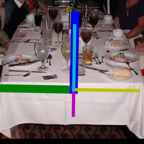
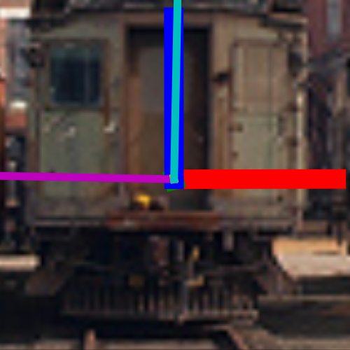
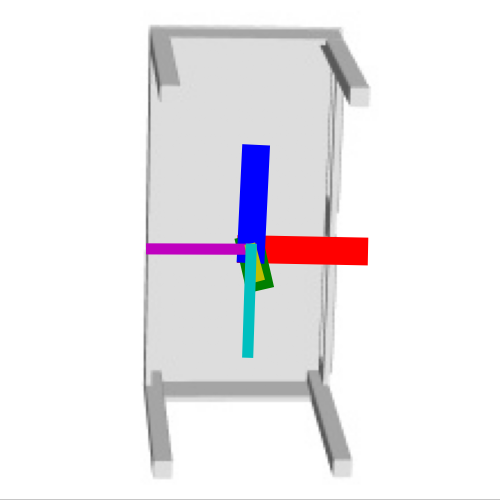
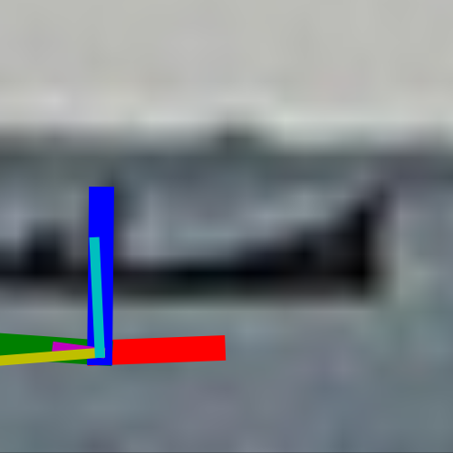
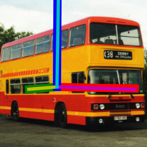
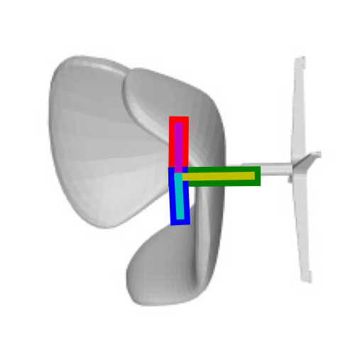
(a)	(b)	(c)	(d)	(e)	(f)

Figure 2: Visualizations of the predicted distributions. The top row displays example images with the projected axes of predictions (thick lines) and ground truths (thin lines) of the object. The bottom row shows the visualization of the corresponding predicted distributions of the image. For clarity we have aligned the predicted poses with the standard axes.

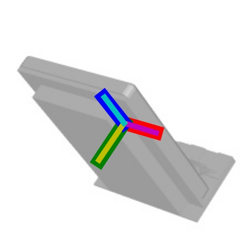
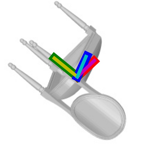
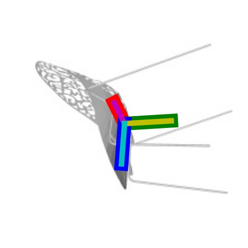
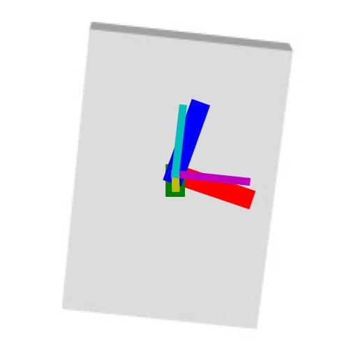
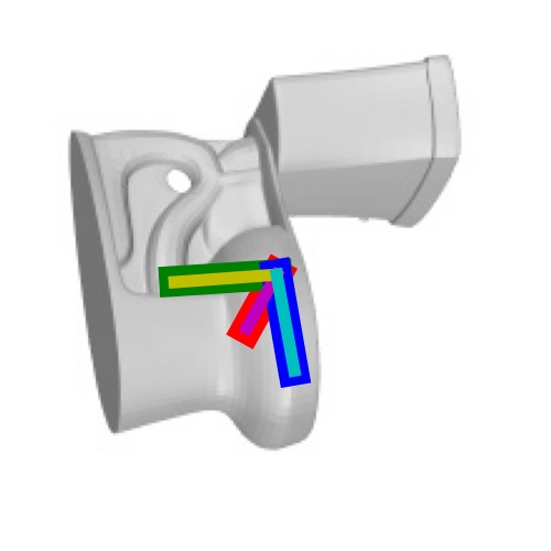
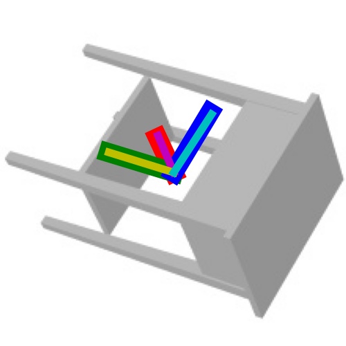
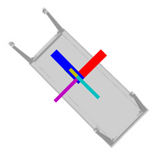
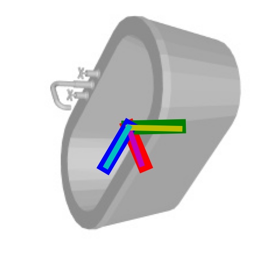
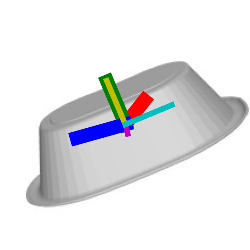
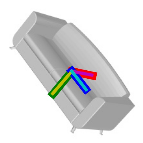
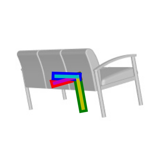
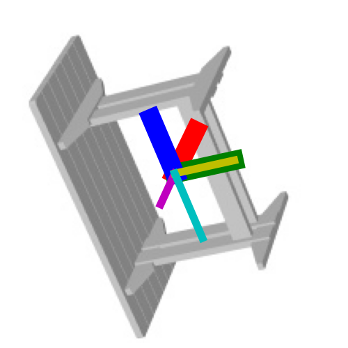
Input image	Distribution visual. [21]	Distribution visual. [20]	Input image	Distribution visual. [21]	Distribution visual. [20]

Figure 3: Visual results on ModelNet10-SO3 dataset. We adopt the distribution visualization methods in [21] and [20]. For input images and visualizations with [21], predicted rotations are shown with thick lines and the ground truths are with thin lines. For visualizations with [20], ground truths are shown by solid circles.

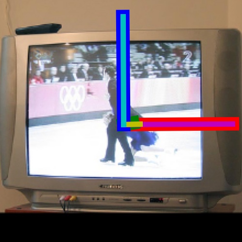
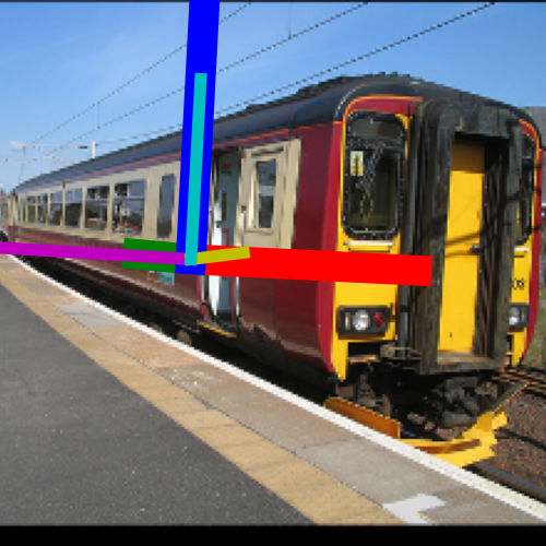
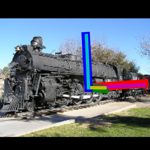
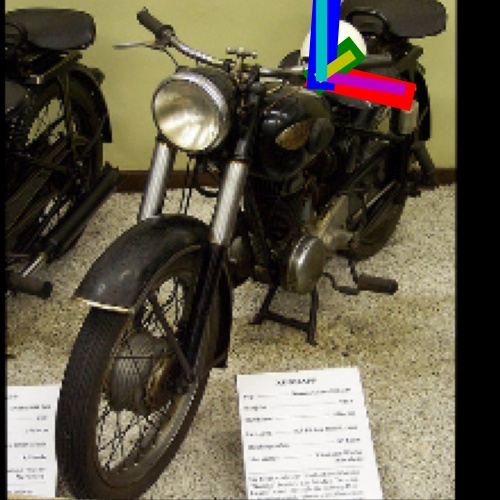
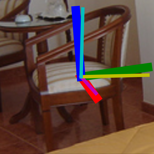
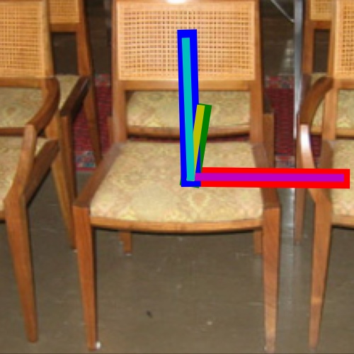
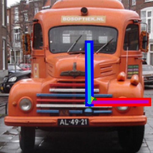
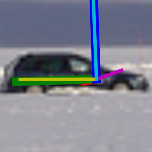
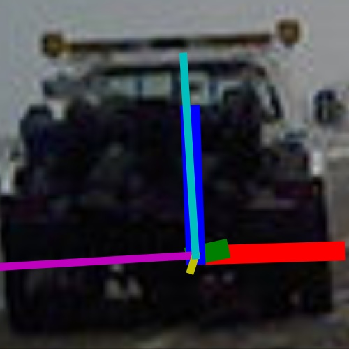
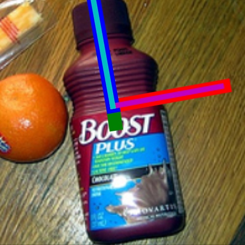
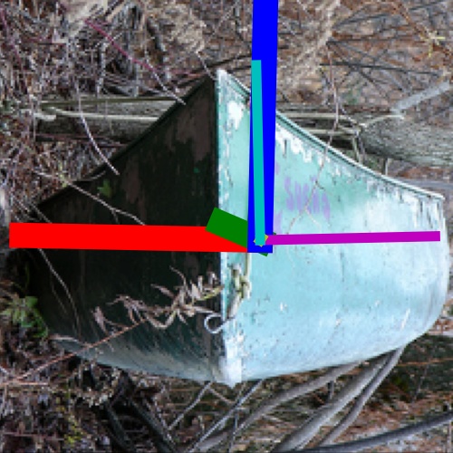
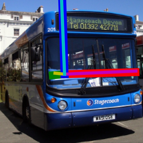
Input image	Distribution visual. [21]	Distribution visual. [20]	Input image	Distribution visual. [21]	Distribution visual. [20]

Figure 4: Visual results on Pascal3D+ dataset. We adopt the distribution visualization methods in [21] and [20]. For input images and visualizations with [21], predicted rotations are shown with thick lines and the ground truths are with thin lines. For visualizations with [20], ground truths are shown by solid circles.

We visualize the predicted distributions in Figure 2 with the visualization method in [21]. The visualization in [21] is achieved by summing the three marginal distributions over the standard basis of $\mathbb{R}^{3}$ and displaying them on the sphere with color coding. As shown in the figure, the predicted distributions can exhibit high uncertainty when the object has rotational symmetry, leading to near 180^∘ errors (a-c), or the input image is with low resolution (d). Subfigure (e-f) show cases with high certainty and reasonably low errors.

We have also included additional visual results on the ModelNet10-SO3 dataset in Figure 3 and the Pascal3D+ dataset in Figure 4. In addition to the visualization technique used in [21], we have included another popular visualization method utilized in [20]. This approach involves discretizing over $\mathrm{SO}(3)$, projecting a great circle of points onto $\mathrm{SO}(3)$ for each point on the 2-sphere, and using the color wheel to indicate the location on the great circle. The probability density is represented by the size of the points on the plot. We recommend consulting the corresponding papers for further details. As depicted in the figures, our distribution provides comprehensive information about the rotation estimations.

5.5 Implementation Details

For fair comparisons, we follow the implementation designs of [21] and merely change the distribution from matrix Fisher distribution to our rotation Laplace distribution. For numerical stability, we clip $\operatorname{tr}(\mathbf{S}-\mathbf{A}^{T}\mathbf{R})$ by $\max(1\mathrm{e}-8,\operatorname{tr}(\mathbf{S}-\mathbf{A}^{T}\mathbf{R}))$ for Eq.13. Please refer to supplementary for more details.

5.6 Comparisons of rotation Laplace Distribution and Quaternion Laplace Distribution

TABLE V: Numerical comparisons with our proposed Quaternion & rotation Laplace distribution and baselines on ModelNet10-SO3 dataset. One model is trained for each category. Quaternion Laplace distribution clearly outperforms Bingham distribution [39].

		Chair			Sofa			Toilet			Bed
	Mean$\downarrow$	Med.$\downarrow$	Acc@5$\uparrow$	Mean$\downarrow$	Med.$\downarrow$	Acc@5$\uparrow$	Mean$\downarrow$	Med.$\downarrow$	Acc@5$\uparrow$	Mean$\downarrow$	Med.$\downarrow$	Acc@5$\uparrow$
Deng et al.[39]	16.5	7.2	0.31	16.5	4.9	0.52	9.6	4.2	0.59	22.0	5.1	0.49
Mohlin et al.[21]	10.8	4.6	0.55	11.1	3.5	0.70	6.4	3.5	0.70	16.0	3.8	0.66
quat. Laplace	12.6	5.2	0.49	13.1	3.7	0.67	5.9	3.4	0.69	17.7	3.4	0.69
rot. Laplace	9.7	3.5	0.68	8.8	2.1	0.84	5.3	2.6	0.83	15.5	2.3	0.82

For the completeness of experiments, we also compare our proposed Quaternion Laplace distribution and Bingham distribution and report the performance in Table V. As shown in the table, Quaternion Laplace distribution consistently achieves superior performance than its competitor, which validates the effectiveness of our Laplace-inspired derivations. However, its rotation error is in general larger than rotation Laplace distribution, since its rotation representation, quaternion, is not a continuous representation, as pointed in [7], thus leading to inferior performance.

6 Analysis of the robustness with Outliers

6.1 Analysis on Gradient w.r.t. Outliers

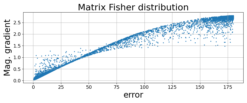
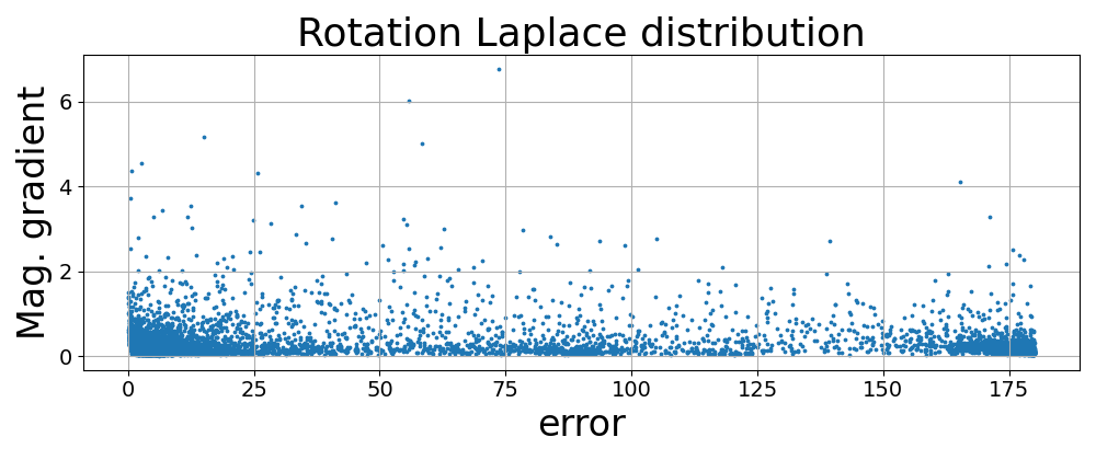
Figure 5: Visualization of the gradient magnituide $\|\partial\mathcal{L}/\partial\text{(distribution param.)}\|$ w.r.t. the prediction errors on ModelNet10-SO3 dataset after convergence.

In the task of rotation regression, predictions with really large errors (e.g., 180^∘ error) are fairly observed due to rotational ambiguity or lack of discriminate visual features. Properly handling these outliers during training is one of the keys to success in probabilistic modeling of rotations.

In Figure 5, for matrix Fisher distribution and rotation Laplace distribution, we visualize the gradient magnitudes $\|\partial\mathcal{L}/\partial\text{(distribution param.)}\|$ w.r.t. the prediction errors on ModelNet10-SO3 dataset after convergence, where each point is a data point in the test set. As shown in the figure, for matrix Fisher distribution, predictions with larger errors clearly yield larger gradient magnitudes, and those with near 180^∘ errors (the outliers) have the biggest impact. Given that outliers may be inevitable and hard to be fixed, they may severely disturb the training process and the sensitivity to outliers can result in a poor fit [18, 35]. In contrast, for our rotation Laplace distribution, the gradient magnitudes are not affected by the prediction errors much, leading to a stable learning process.

Consistent results can also be seen in Figure 1 of the main paper, where the red dots illustrate the sum of the gradient magnitude over the population within an interval of prediction errors. We argue that, at convergence, the gradient should focus more on the large population with low errors rather than fixing the unavoidable large errors.

6.2 Experiments on ModelNet10-SO3 Dataset with Outlier Injections

To further demonstrate the robustness of our distribution, we manually inject outliers to the perfectly labeled synthetic dataset and compare rotation Laplace distribution with matrix Fisher distribution. Specifically, we randomly choose 1%, 5%, 10% and 30% images from the training set of ModelNet10-SO3 dataset respectively, and apply a random rotation in $\mathrm{SO}(3)$ to the given ground truth. Thus, the chosen images become outliers in the dataset due to the perturbed annotations. We fix the processed dataset for different methods.

The results on the perturbed dataset are shown in Table VI and Figure 6, where our method consistently outperforms matrix Fisher distribution under different levels of perturbations. More importantly, as shown in Figure 6, our method clearly better tolerates the outliers, resulting in less performance degradation and remains a reasonable performance even under intense perturbations. For example, Acc@30^∘ of matrix Fisher distribution greatly drops from 0.751 to 0.467 with 30% outliers, while that of our method merely goes down from 0.770 to 0.700, which shows the superior robustness of our method.

TABLE VI: Comparisons on the perturbed ModelNet10-SO3 dataset where random outliers are injected.

Outlier Inject	Method	Acc@3∘$\uparrow$	Acc@5∘$\uparrow$	Acc@10∘$\uparrow$	Acc@15∘$\uparrow$	Acc@30∘$\uparrow$	Med.(∘)$\downarrow$
0%	Mohlin et al.[21]	0.164	0.389	0.615	0.684	0.751	17.9
	rotation Laplace	0.446	0.613	0.714	0.741	0.770	12.2
1%	Mohlin et al.[21]	0.141	0.336	0.589	0.664	0.740	20.5
	rotation Laplace	0.429	0.601	0.711	0.739	0.769	12.4
5%	Mohlin et al.[21]	0.0818	0.229	0.501	0.605	0.711	24.8
	rotation Laplace	0.368	0.561	0.693	0.727	0.762	12.6
10%	Mohlin et al.[21]	0.0493	0.151	0.403	0.536	0.677	26.8
	rotation Laplace	0.329	0.523	0.668	0.706	0.747	16.1
30%	Mohlin et al.[21]	0.0063	0.0255	0.126	0.243	0.467	45.3
	rotation Laplace	0.151	0.345	0.565	0.634	0.700	22.7

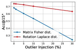
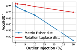
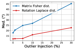
Figure 6: Comparisons on the perturbed ModelNet10-SO3 dataset where random outliers are injected. The horizontal axis is the percentage of perturbed images, and the vertical axis represents the corresponding metric.

7 Analysis of the robustness with Noise

Mathematically, our rotation Laplace distribution benefits from the heavy-tail nature of the distribution, which introduces a small gradient when the difference between prediction and label is large, resulting in its robustness to outliers. However, one possible trade-off is that when the prediction is close to the label, the gradient is large, which could result in the wrong gradient dominating the training process in scenarios with slight noise. To investigate this issue, we experiment with perturbed data that includes small noise injections in 7.1. We further evaluate and apply the robustness to the semi-supervised rotation regression task where pseudo labels are noisy in 7.2.

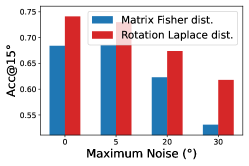
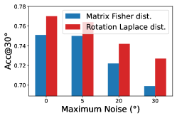
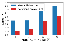
Figure 7: Comparisons on the perturbed ModelNet10-SO3 dataset where random noise are injected and fixed. The horizontal axis is the maximum noise, and the vertical axis represents the corresponding metric.

7.1 Experiments on ModelNet10-SO3 Dataset with Noise Injections

Noises on dataset labels, such as human labeling errors, can cause overfitting on imperfect training sets and lead to poor performance during testing. To assess the robustness of our rotation Laplace distribution to such noise, we perturb ModelNet10-SO3 with an injection of random noise and compare the performance of our rotation Laplace with baseline under this noisy condition. Specifically, we generate random rotation in the form of the axis-angle representation where the axis direction and the angle’s magnitude are sampled from uniform distributions on the unit sphere $\mathrm{S}^{2}$ and $\left[0,u\right]$, respectively. The upper bound of the magnitude $u$ was set to 5^∘, 20^∘, and 30^∘ in the following experiments. We add this random rotation to all training data labels as noise and fixed the processed dataset for different methods.

TABLE VII: Comparisons on the perturbed ModelNet10-SO3 dataset where random noise are injected and fixed.

Metric	Method	Maximum Noise (∘)
		0	5	20	30
Acc@15∘$\uparrow$	Mohlin et al.[21]	0.684	0.683	0.623	0.531
	rotation Laplace	0.741	0.730	0.674	0.618
Acc@30∘$\uparrow$	Mohlin et al.[21]	0.751	0.750	0.722	0.699
	rotation Laplace	0.770	0.764	0.742	0.727
Med.(∘)$\downarrow$	Mohlin et al.[21]	17.9	18.0	23.2	25.8
	rotation Laplace	12.2	13.4	17.7	20.5

TABLE VIII: Comparisons on the perturbed ModelNet10-SO3 dataset where dynamically changing noise are injected.

Metric	Method	Maximum Noise (∘)
		0	5	20	30
Acc@15∘$\uparrow$	Mohlin et al.[21]	0.684	0.682	0.678	0.667
	rotation Laplace	0.741	0.737	0.717	0.708
Acc@30∘$\uparrow$	Mohlin et al.[21]	0.751	0.753	0.745	0.745
	rotation Laplace	0.770	0.770	0.761	0.764
Med.(∘)$\downarrow$	Mohlin et al.[21]	17.9	16.8	17.7	17.1
	rotation Laplace	12.2	12.0	13.6	13.1

The results on the perturbed dataset are presented in Table VII and Figure 7, where our method consistently outperforms matrix Fisher distribution under different levels of perturbations. For instance, at a maximum human labeling noise of 5^∘ and 30^∘, Acc@15^∘ of our methods outperforms that of the matrix Fisher distribution by 4.7% and 8.7%. Our method maintains reasonable performance even under relatively severe perturbations, indicating its superior practical value in real-world scenarios involving human labeling errors.

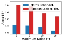
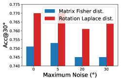
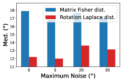
Figure 8: Comparisons on the perturbed ModelNet10-SO3 dataset where dynamically changing noise are injected. The horizontal axis is the maximum noise, and the vertical axis represents the corresponding metric.

We also perform experiments by introducing dynamically changing noise into the ground truth labels, simulating the use of pseudo-labeling in semi-supervised learning as discussed in Section 7.2. In this experiment, we regenerate random rotation noise each epoch using the same method as before, with an upper bound of 5^∘, 20^∘, and 30^∘. This approach allows us to evaluate the robustness of the rotation Laplace and matrix Fisher distributions under noisy while evolving labels.

Table VIII and Figure 8 present the quantitative comparisons of our rotation Laplace distribution and the matrix Fisher distribution on the perturbed ModelNet10-SO3 dataset, where dynamically changing noise is injected. Notably, our method consistently outperforms the matrix Fisher distribution in scenarios with both small and relatively large levels of dynamically changing noise while maintaining a reasonable margin. And both methods demonstrate better performance than training on a fixed perturbed dataset, for this setting alleviates overfitting on noisy training sets.

Although our method achieves good performance under various levels of dynamic noise, we observed that in some cases, training results with large noise may slightly outperform those with small noise with some measure. For example, the median error is lower when the maximum noise is 5^∘ compared to when there is no noise, and the Acc@15^∘ is higher when the maximum noise is 30^∘ compared to 20^∘. This can be attributed to the fact that dynamic noise makes the labels smoother to some extent, which achieves data augmentation through jittering. However, this situation is limited to cases where the noise gap is small. When the noise gap is large, training performance is still better with low noise levels, as evidenced by the comparison between no noise and 30^∘ noise.

7.2 Application on Semi-supervised Rotation Regression

One of the major obstacles to improving rotation regression is expensive rotation annotations. Though many large-scale image datasets have been curated with sufficient semantic annotations, obtaining a large-scale real dataset with rotation annotations can be extremely laborious, expensive and error-prone[63]. To reduce the amount of supervision, Yin et al. proposed FisherMatch[3] to learn regressor of matrix Fisher distribution from minor labeled data and a large amount of unlabeled data, namely semi-supervised learning. The core method is based on pseudo-labeling and further leverages the entropy of matrix Fisher distribution as uncertainty to filter low-quality pseudo-labels. According to our prior analysis, our method still demonstrates satisfactory performance in scenarios with dynamically changing noise. Therefore, it is more appropriate to utilize it for training scenes that involve the use of pseudo-labeling with minimal errors. In light of this, we incorporate rotation Laplace distribution into the framework of FisherMatch to evaluate its applicability in semi-supervised rotation regression tasks.

7.2.1 Uncertainty quantification measured by distribution entropy

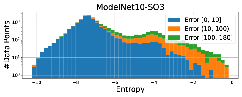
Figure 9: Visualization of the indication ability of the distribution entropy w.r.t. the performance. The horizontal axis is the distribution entropy and the vertical axis is the number of data points (in log scale), color coded by the errors (in degrees). The experiments are done on the test set of ModelNet10-SO3 dataset (left) and Pascal3D+ dataset (right).

Probabilistic modeling of rotation naturally models the uncertainty information of rotation regression. Yin et al.[3] proposes to use the entropy of the distribution as an uncertainty measure. We adopt it as the uncertainty indicator of rotation Laplace distribution and plot the relationship between the error of the prediction and the corresponding distribution entropy on the testset of ModelNet10-SO3 in Figure 9. As shown in the figure, predictions with lower entropies (i.e., lower uncertainty) clearly achieve higher accuracy than predictions with large entropies, demonstrating the ability of uncertainty estimation of our rotation Laplace distribution. We compute the entropy via discretization, where $\mathrm{SO}(3)$ space is quantized into a finite set of equivolumetric girds $\mathcal{G}=\{\mathbf{R}|\mathbf{R}\in\mathrm{SO}(3)\}$, and

$$\scriptsize H\left(p\right)=-\int_{\mathrm{SO}(3)}p\log p\mathrm{d}\mathbf{R}\approx-\sum_{\mathbf{R}_{i}\in\mathcal{G}}p_{i}\log p_{i}\Delta\mathbf{R}_{i}$$

We use about 0.3M grids to discretize $\mathrm{SO}(3)$ space.

TABLE IX: Comparing our method with the baselines under different ratios of labeled data for semi-supervised rotation regression.

Category	Method	5%		10%
		Mean(∘)	Med.(∘)	Mean(∘)	Med.(∘)
Sofa	SSL-9D-Consist.	36.86	8.65	25.94	6.81
	SSL-FisherMatch	31.09	7.55	21.16	5.21
	SSL-rot.Laplace	26.12	6.07	19.32	4.25
Chair	SSL-9D-Consist.	31.20	11.29	23.59	8.10
	SSL-FisherMatch	26.45	9.65	20.18	7.63
	SSL-rot.Laplace	23.66	8.51	18.35	6.75

7.2.2 Revisit FisherMatch

FisherMatch leverages a teacher-student mutual learning framework composed of a learnable student model and an exponential-moving-average (EMA) teacher model. A training batch for this framework contains a mixture of $\left\{\boldsymbol{x}_{i}^{l}\right\}_{i=1}^{B_{l}}$ labeled samples and $\left\{\boldsymbol{x}_{i}^{u}\right\}_{i=1}^{B_{u}}$ unlabeled samples.

On labeled data, the student network is trained by the ground-truth labels with the supervised loss; while on unlabeled data, the student model takes the pseudo labels from the EMA teacher. An entropy-based filtering technique is leveraged to filter out noisy teacher predictions. The overall loss term is as follows:

$$L_{ssl}=L_{l}\left(\boldsymbol{x}^{l},\boldsymbol{y}^{l}\right)+\lambda_{u}L_{u}\left(\boldsymbol{x}^{u}\right)$$ (10)

where $\lambda_{u}$ is the unsupervised loss weight.

For pseudo label filtering, a fixed entropy threshold $\tau$ is set, and the prediction will be reserved as a pseudo label only if its entropy is lower than the threshold. We denote rotation regressor as $\Phi$ that takes a single RGB image $\boldsymbol{x}$ as input and $\mathcal{MF}$ as matrix Fisher distribution. Specifically, for unlabeled data $\boldsymbol{x}^{u}$, assume $p_{t}=\mathcal{MF}(\mathbf{A}^{u}_{t})$ is the teacher output with $\mathbf{A}^{u}_{t}=\mathbf{\Phi}_{t}(\boldsymbol{x}^{u})$ and $p_{s}=\mathcal{MF}(\mathbf{A}^{u}_{s})$ is the student output with $\mathbf{A}^{u}_{s}=\mathbf{\Phi}_{s}(\boldsymbol{x}^{u})$ , the loss on unlabeled data is therefore:

$$L_{u}\left(\boldsymbol{x}^{u}\right)=\mathbbm{1}\left(H(p_{t})\leq\tau\right)L_{u}\left(p_{t},p_{s}\right)$$ (11)

We recommend the readers to [3] for more details.

7.2.3 Incorperating rotation Laplace into FisherMatch

Note that FisherMatch is a framework independent of probabilistic distribution of rotation, we can simply replace the matrix Fisher distribution with our rotation Laplace distribution. According to Equ 11, we can derive unsupervised loss as follows:

$$L_{u}\left(\boldsymbol{x}^{u}\right)=\mathbbm{1}\left(H(\mathcal{RL}(\mathbf{A}^{u}_{t}))\leq\tau\right)L\left(\mathcal{RL}(\mathbf{A}^{u}_{t}),\mathcal{RL}(\mathbf{A}^{u}_{t})\right)$$ (12)

Specifically, we use NLL loss for supervised loss similar to Sec.5 and CE (cross entropy) loss for unsupervised loss in Eq. 12.

We conduct experiment on ModelNet10-SO3 dataset, following the same semi-supervised learning setting in FisherMatch, which uses MobileNet-V2[65] architecture and Adam optimizer. Both the baselines come from Yin et al.[3] due to they are the unique work to tackle semi-supervised rotation regression on SO(3). SSL-L1-Consistency refers to adopting the teacher-student mutual learning framework which applies L1 loss as the consistency supervision between the student and teacher predictions without filtering.

The experimental results in Table IX indicate that our method consistently outperforms both baselines and achieves a significant improvement over FisherMatch in both 5% and 10% labeled data scenarios. Specifically, for the sofa class at a 5% label ratio, our method reduces the mean error by 4.97^∘ and the median error by 1.48^∘. These results demonstrate the superior noise-robustness of our rotation Laplace distribution for semi-supervised learning.

8 Multimodal prediction with rotation Laplace mixture model

For the purpose of capturing multimodal rotation space, especially with symmetric objects, we extend rotation Laplace distribution into rotation Laplace mixture model.

8.1 rotation Laplace mixture model

rotation Laplace mixture model can be built upon a set of single-modal rotation Laplace distributions by assigning a weight factor for each component and combining them linearly. In this way, each unimodal component may capture one plausible solution to the corresponding task and the mixture model takes multi-modality into account and covers a broader solution space.

Definition 5.

rotation Laplace mixture model. The random variable $\mathbf{R}\in\mathrm{SO}(3)$ follows rotation Laplace mixture model with parameter $\mathcal{A}=\{\mathbf{A}_{i}\}_{i=1}^{M}$ and weights $\mathcal{W}=\{w_{i}\}_{i=1}^{M}$, if its probability density function is defined as

$$p(\mathbf{R};\mathcal{A},\mathcal{W}) =\sum_{i=1}^{M}w_{i}\cdot p(\mathbf{R};\mathbf{A}_{i})$$ (13)

$$=\sum_{i=1}^{M}\frac{w_{i}}{F(\mathbf{A}_{i})}\frac{\exp\left(-\sqrt{\operatorname{tr}\left(\mathbf{S}_{i}-\mathbf{A}_{i}^{T}\mathbf{R}\right)}\right)}{\sqrt{\operatorname{tr}\left(\mathbf{S}_{i}-\mathbf{A}_{i}^{T}\mathbf{R}_{i}\right)}}$$

where $M$ is the number of components, $w_{i}\in[0,1]$ is the scalar weight of each component, and

$$\sum_{i=1}^{M}w_{i}=1$$

$\mathbf{A}_{i}\in\mathbb{R}^{3\times 3}$ is an unconstrained matrix, and $\mathbf{S}_{i}$ is the diagonal matrix composed of the proper singular values of matrix $\mathbf{A}_{i}$, i.e., $\mathbf{A}_{i}=\mathbf{U}_{i}\mathbf{S}_{i}\mathbf{V}_{i}^{T}$. We also denote rotation Laplace mixture model as $\mathbf{R}\sim\mathcal{RL}_{mix}(\mathcal{A},\mathcal{W})$.

8.2 Loss function

Mixture rotation Laplace loss Similar to Eq. 8, we define mixture rotation Laplace loss as the negative log-likelihood (NLL) of the distribution of the mixture model, as follows:

$$\mathcal{L}_{\text{nll}}(\boldsymbol{x},\mathbf{R}_{\boldsymbol{x}})=-\log p\left(\mathbf{R}_{\boldsymbol{x}};\mathcal{A}_{\boldsymbol{x}},\mathcal{W}_{\boldsymbol{x}}\right)$$ (14)

where $\mathcal{A}_{\boldsymbol{x}}$ and $\mathcal{W}_{\boldsymbol{x}}$ are predicted by the network. Mixture rotation Laplace loss can be viewed as the linear combination of the NLL loss of each component.

In theory, mixture rotation Laplace loss is sufficient for capturing the multi-modality of the solution space. However, as pointed out by previous works [66, 28], directly optimizing with the NLL loss of the mixture model can lead to numerical instabilities and mode collapse. Thus a proper technique used for encouraging diverging predictions is crucial.

Winner-Take-ALL loss Inspired by [39], we incoporate a “Winner-Take-All” (WTA) strategy in our training process, which has been shown to be effective with multimodal scenarios [67, 68]. In concrete, in WTA strategy, we only update the branch with highest probability density function of ground truth and leave the other branches unchanged. This provably leads to the Voronoi tesselation of the output space [39].

Denote $\mathcal{RL}_{i}$ as the i-th component of the mixture model. We first select the “winner” branch by checking the pdf of ground truth $\mathbf{R}_{\boldsymbol{x}}$:

$$i^{*}=\underset{i}{\arg\max}\mathcal{RL}_{i}\left(\mathbf{R}_{\boldsymbol{x}};\mathbf{A}_{i}\right)$$ (15)

And then optimizing this branch with NLL loss (Eq. 8):

$$\mathcal{L}_{WTA}=\mathcal{L}_{i^{*}}(\boldsymbol{x},\mathbf{R}_{\boldsymbol{x}})$$ (16)

In addition, Rupprecht et al. [67] find that a relaxted version of WTA which allows a small portion of gradient for unselected branches will help with training by avoiding “dead” branches which never get updated due to the bad initialization. Thus we use the relaxed WTA strategy:

$$\mathcal{L}_{RWTA}=\sum_{i=1}^{M}\pi_{i}\mathcal{L}_{i}(\boldsymbol{x},\mathbf{R}_{\boldsymbol{x}})$$ (17)

$$\pi_{i}=\begin{cases}1-\epsilon&i=i^{*}\\ \frac{\epsilon}{M-1}&\text{ others }\end{cases}$$

We use $\epsilon=0.05$ in experiments. RWTA loss guides our mixture model to better cover different modes of solution space.

The overall loss of rotation Laplace mixture model is defined as follows

$$\mathcal{L}_{\text{mix}}=\mathcal{L}_{\text{nll}}+\lambda\mathcal{L}_{\text{RWTA}}$$ (18)

We set $\lambda=1$ in experiments.

8.3 Experiments with rotation Laplace Mixture Model

We validate rotation Laplace mixture model on the task of object rotation estimation, similar to Sec. 5. To better evaluate the multi-modality property of the distributions, we follow IPDF [20] to use top-k metrics where the best results from k candidates are reported.

8.3.1 Top-k Metrics

Since only a single ground truth is available, for symmetric objects, the precision metrics can be misleading because they may penalize correct predictions that do not have a corresponding annotation. We follow IPDF [20] to use top-k metrics: $N$ pose candidates are predicted by the mixture model, and the best results of the $k$ ($k\leq N$) predictions are reported. We set $N=4$ and $k=2,4$ as IPDF. Note that we only train one model with $N$ branches without the burden to re-train it for every specified $k$.

8.3.2 Quantitative Results

TABLE X: Numerical comparisons on multimodal probabilistic distributions with top-k metrics on ModelNet10-SO3 dataset averaged on all categories.

		Acc@15∘$\uparrow$	Acc@30∘$\uparrow$	Med$\downarrow$
Single modal	Deng et al.[39]	0.562	0.694	32.6
	Mohlin et al.[21]	0.693	0.757	17.1
	Murphy et al.[20]	0.719	0.735	21.5
	rotation Laplace	0.742	0.772	12.7
Top-2	Deng et al.[39]	0.863	0.897	3.8
	Mohlin et al.[21]	0.864	0.903	3.8
	Murphy et al.[20]	0.868	0.888	4.9
	rotation Laplace	0.900	0.918	2.3
Top-4	Deng et al.[39]	0.875	0.915	3.7
	Mohlin et al.[21]	0.882	0.926	3.7
	Murphy et al.[20]	0.904	0.926	4.8
	rotation Laplace	0.919	0.940	2.2

We compare our rotation Laplace distribution with other probabilistic baselines on all categories of ModelNet10-SO3 dataset, and the results are reported in Tab X. Shown in the table, the performance of all methods increases dramatically when we allow for $k$ (even when $k=2$) candidates, which demonstrate the advantage of taking multi-modality into account.

Besides superior performance with single modal output, our rotation Laplace distribution also performs the best among all the baselines under all metrics in both top-2 and top-4 settings, which validates the feasibility and effectiveness of rotation Laplace mixture model.

8.3.3 Qualitative Results

Input image	Prediction of each branche

Figure 10: Visualizations of the predicted distributions of rotation Laplace mixture model. The first column displays the input images and the remaining columns show predicted distributions of each branch.

In Figure 10, we visualize the output distributions of each branch of rotation Laplace mixture model, and demonstrate how our model is able to capture different modes with ambiguous inputs. Shown in the first three rows, for objects with rotational symmetries, e.g., bathtub, the multi-hypothesis predictions well present the plausible solution space of the input. While in cases where an object does not carry ambiguity, illustrated in the last two rows, different branches tend to agree with each other and correctly collapse to a single mode.

9 Conclusion

In this paper, we draw inspiration from multivariant Laplace distribution and derive a novel distribution for probabilistic rotation regression, namely, rotation Laplace distribution. We demonstrate that our distribution is robust to the disturbance of both outliers and small noises, thus achieving significantly superior performance on supervised and semi-supervised rotation regression tasks over all the baselines. We also extend rotation Laplace distribution to rotation Laplace mixture model to better capture the multi-modal rotation space. Extensive comparisons with both probabilistic and non-probabilistic baselines demonstrate the effectiveness and advantages of our proposed distribution.

Yingda Yin is a Ph.D. student at School of Computer Science, Peking University. His research interests lie in 3D computer vision, including rotation modeling, object pose estimation and camera localization.

Jiangran Lyu is currently working toward the PhD degree in computer science at Peking University. His current research span 3D computer vision and robotics, with a special interest in embodied AI.

Yang Wang is an Undergraduate student at School of EECS, Peking University. His research interests are focused on the field of 3D vision, including rotation regression, object pose estimation and 3D reconstruction.

He Wang is a tenure-track assistant professor in the Center on Frontiers of Computing Studies (CFCS) at Peking University, where he founds and leads Embodied Perception and InteraCtion (EPIC) Lab. His research interests span 3D vision, robotics, and machine learning, with a special focus on embodied AI. His research objective is to endow robots working in complex real-world scenes with generalizable 3D vision and interaction policies in a scalable way. He has published more than 40 papers on top conferences and journals of computer vision, robotics and learning, including CVPR/ICCV/ECCV/TRO/ICRA/IROS/NeurIPS/ICLR/AAAI. His pioneering work on category-level 6D pose estimation, NOCS, receives 2022 World Artificial Intelligence Conference Youth Outstanding Paper (WAICYOP) Award and his work also receives ICRA 2023 outstanding manipulation finalist and Eurographics 2019 best paper honorable mention. He serves as an associate editor of Image and Vision Computing and serves area chairs in CVPR 2022 and WACV 2022. Prior to joining Peking University, he received his Ph.D. degree from Stanford University in 2021 under the advisory of Prof. Leonidas J. Guibas and his Bachelor’s degree in 2014 from Tsinghua University.

Baoquan Chen is a Professor of Peking University, where he is the Associate Dean of the School of Artificial Intelligence. For his contribution to spatial data (modeling) and visualization, he was elected IEEE Fellow 2020. His research interests generally lie in computer graphics, visualization, and human-computer interaction, focusing specifically on large-scale city modeling, simulation and visualization. He has published more than 200 papers in international journals and conferences, including 40+ papers in ACM Transactions on Graphics (TOG)/SIGGRAPH/SIGGRAPH Asia. Chen serves/served as associate editor of ACM TOG/IEEE Transactions on Visualization and Graphics (TVCG), and has served as conference steering committee member (ACM SIGGRAPH Asia, IEEE VIZ), conference chair (SIGGRAPH Asia 2014, IEEE Visualization 2005), program chair (IEEE Visualization 2004), as well as program committee member of almost all conferences in the visualization and computer graphics fields for numerous times. Prior to the current post, he was, Dean, School of Computer Science and Technology, SDU. Chen received an MS in Electronic Engineering from Tsinghua University, Beijing (1994), and a second MS (1997) and then PhD (1999) in Computer Science from the State University of New York at Stony Brook.

References

- [1] R. Morris, L. Rubin, and H. Tirri, “Neural network techniques for object orientation detection. solution by optimal feedforward network and learning vector quantization approaches,” IEEE Transactions on Pattern Analysis and Machine Intelligence, vol. 12, no. 11, pp. 1107–1115, 1990.
- [2] H. Wang, S. Sridhar, J. Huang, J. Valentin, S. Song, and L. J. Guibas, “Normalized object coordinate space for category-level 6d object pose and size estimation,” in Proceedings of the IEEE/CVF Conference on Computer Vision and Pattern Recognition, 2019, pp. 2642–2651.
- [3] Y. Yin, Y. Cai, H. Wang, and B. Chen, “Fishermatch: Semi-supervised rotation regression via entropy-based filtering,” in Proceedings of the IEEE/CVF Conference on Computer Vision and Pattern Recognition, 2022, pp. 11 164–11 173.
- [4] S. Dong, Q. Fan, H. Wang, J. Shi, L. Yi, T. Funkhouser, B. Chen, and L. J. Guibas, “Robust neural routing through space partitions for camera relocalization in dynamic indoor environments,” in Proceedings of the IEEE/CVF Conference on Computer Vision and Pattern Recognition, 2021, pp. 8544–8554.
- [5] M. Breyer, J. J. Chung, L. Ott, R. Siegwart, and J. Nieto, “Volumetric grasping network: Real-time 6 dof grasp detection in clutter,” arXiv preprint arXiv:2101.01132, 2021.
- [6] H. Ci, X. Ma, C. Wang, and Y. Wang, “Locally connected network for monocular 3d human pose estimation,” IEEE Transactions on Pattern Analysis and Machine Intelligence, vol. 44, no. 3, pp. 1429–1442, 2022.
- [7] Y. Zhou, C. Barnes, J. Lu, J. Yang, and H. Li, “On the continuity of rotation representations in neural networks,” in Proceedings of the IEEE/CVF Conference on Computer Vision and Pattern Recognition, 2019, pp. 5745–5753.
- [8] J. Levinson, C. Esteves, K. Chen, N. Snavely, A. Kanazawa, A. Rostamizadeh, and A. Makadia, “An analysis of svd for deep rotation estimation,” Advances in Neural Information Processing Systems, vol. 33, pp. 22 554–22 565, 2020.
- [9] J. Chen, Y. Yin, T. Birdal, B. Chen, L. J. Guibas, and H. Wang, “Projective manifold gradient layer for deep rotation regression,” in Proceedings of the IEEE/CVF Conference on Computer Vision and Pattern Recognition, 2022, pp. 6646–6655.
- [10] J. L. Crassidis and F. L. Markley, “Unscented filtering for spacecraft attitude estimation,” Journal of guidance, control, and dynamics, vol. 26, no. 4, pp. 536–542, 2003.
- [11] R. McAllister, Y. Gal, A. Kendall, M. Van Der Wilk, A. Shah, R. Cipolla, and A. Weller, “Concrete problems for autonomous vehicle safety: Advantages of bayesian deep learning.” International Joint Conferences on Artificial Intelligence, Inc., 2017.
- [12] G. Singh, S. Akrigg, M. D. Maio, V. Fontana, R. J. Alitappeh, S. Khan, S. Saha, K. Jeddisaravi, F. Yousefi, J. Culley, T. Nicholson, J. Omokeowa, S. Grazioso, A. Bradley, G. D. Gironimo, and F. Cuzzolin, “Road: The road event awareness dataset for autonomous driving,” IEEE Transactions on Pattern Analysis and Machine Intelligence, vol. 45, no. 1, pp. 1036–1054, 2023.
- [13] Q. Fang, Y. Yin, Q. Fan, F. Xia, S. Dong, S. Wang, J. Wang, L. Guibas, and B. Chen, “Towards accurate active camera localization,” arXiv e-prints, pp. arXiv–2012, 2020.
- [14] P. Wei, Y. Zhao, N. Zheng, and S.-C. Zhu, “Modeling 4d human-object interactions for joint event segmentation, recognition, and object localization,” IEEE Transactions on Pattern Analysis and Machine Intelligence, vol. 39, no. 6, pp. 1165–1179, 2017.
- [15] C. Bingham, “An antipodally symmetric distribution on the sphere,” The Annals of Statistics, pp. 1201–1225, 1974.
- [16] C. Khatri and K. V. Mardia, “The von mises–fisher matrix distribution in orientation statistics,” Journal of the Royal Statistical Society: Series B (Methodological), vol. 39, no. 1, pp. 95–106, 1977.
- [17] M. J. Prentice, “Orientation statistics without parametric assumptions,” Journal of the Royal Statistical Society: Series B (Methodological), vol. 48, no. 2, pp. 214–222, 1986.
- [18] K. P. Murphy, Machine learning: a probabilistic perspective. MIT press, 2012.
- [19] H. Yang and L. Carlone, “Certifiably optimal outlier-robust geometric perception: Semidefinite relaxations and scalable global optimization,” IEEE Transactions on Pattern Analysis and Machine Intelligence, vol. 45, no. 3, pp. 2816–2834, 2023.
- [20] K. A. Murphy, C. Esteves, V. Jampani, S. Ramalingam, and A. Makadia, “Implicit-pdf: Non-parametric representation of probability distributions on the rotation manifold,” in International Conference on Machine Learning. PMLR, 2021, pp. 7882–7893.
- [21] D. Mohlin, J. Sullivan, and G. Bianchi, “Probabilistic orientation estimation with matrix fisher distributions,” Advances in Neural Information Processing Systems, vol. 33, pp. 4884–4893, 2020.
- [22] N. Mitianoudis, “A generalized directional laplacian distribution: Estimation, mixture models and audio source separation,” IEEE Transactions on Audio, Speech, and Language Processing, vol. 20, no. 9, pp. 2397–2408, 2012.
- [23] L. Muñoz-Gonzalez, M. Lázaro-Gredilla, and A. R. Figueiras-Vidal, “Laplace approximation for divisive gaussian processes for nonstationary regression,” IEEE Transactions on Pattern Analysis and Machine Intelligence, vol. 38, no. 3, pp. 618–624, 2016.
- [24] I. Goodfellow, Y. Bengio, and A. Courville, Deep learning. MIT press, 2016.
- [25] D. A. Nix and A. S. Weigend, “Estimating the mean and variance of the target probability distribution,” in Proceedings of 1994 ieee international conference on neural networks (ICNN’94), vol. 1. IEEE, 1994, pp. 55–60.
- [26] A. Kendall and Y. Gal, “What uncertainties do we need in bayesian deep learning for computer vision?” Advances in neural information processing systems, vol. 30, 2017.
- [27] B. Lakshminarayanan, A. Pritzel, and C. Blundell, “Simple and scalable predictive uncertainty estimation using deep ensembles,” Advances in neural information processing systems, vol. 30, 2017.
- [28] O. Makansi, E. Ilg, O. Cicek, and T. Brox, “Overcoming limitations of mixture density networks: A sampling and fitting framework for multimodal future prediction,” in Proceedings of the IEEE/CVF Conference on Computer Vision and Pattern Recognition, 2019, pp. 7144–7153.
- [29] E. Ilg, O. Cicek, S. Galesso, A. Klein, O. Makansi, F. Hutter, and T. Brox, “Uncertainty estimates and multi-hypotheses networks for optical flow,” in Proceedings of the European Conference on Computer Vision (ECCV), 2018, pp. 652–667.
- [30] D. B. de Jong, F. Paredes-Vallés, and G. C. H. E. de Croon, “How do neural networks estimate optical flow? a neuropsychology-inspired study,” IEEE Transactions on Pattern Analysis and Machine Intelligence, vol. 44, no. 11, pp. 8290–8305, 2022.
- [31] M. Poggi, F. Aleotti, F. Tosi, and S. Mattoccia, “On the uncertainty of self-supervised monocular depth estimation,” in Proceedings of the IEEE/CVF Conference on Computer Vision and Pattern Recognition, 2020, pp. 3227–3237.
- [32] X. Qi, Z. Liu, R. Liao, P. H. S. Torr, R. Urtasun, and J. Jia, “Geonet++: Iterative geometric neural network with edge-aware refinement for joint depth and surface normal estimation,” IEEE Transactions on Pattern Analysis and Machine Intelligence, vol. 44, no. 2, pp. 969–984, 2022.
- [33] B. Wang, J. Lu, Z. Yan, H. Luo, T. Li, Y. Zheng, and G. Zhang, “Deep uncertainty quantification: A machine learning approach for weather forecasting,” in Proceedings of the 25th ACM SIGKDD International Conference on Knowledge Discovery & Data Mining, 2019, pp. 2087–2095.
- [34] J. Li, S. Bian, A. Zeng, C. Wang, B. Pang, W. Liu, and C. Lu, “Human pose regression with residual log-likelihood estimation,” in Proceedings of the IEEE/CVF International Conference on Computer Vision, 2021, pp. 11 025–11 034.
- [35] D. S. Nair, N. Hochgeschwender, and M. A. Olivares-Mendez, “Maximum likelihood uncertainty estimation: Robustness to outliers,” arXiv preprint arXiv:2202.03870, 2022.
- [36] S. Prokudin, P. Gehler, and S. Nowozin, “Deep directional statistics: Pose estimation with uncertainty quantification,” in Proceedings of the European conference on computer vision (ECCV), 2018, pp. 534–551.
- [37] K. V. Mardia, P. E. Jupp, and K. Mardia, Directional statistics. Wiley Online Library, 2000, vol. 2.
- [38] I. Gilitschenski, R. Sahoo, W. Schwarting, A. Amini, S. Karaman, and D. Rus, “Deep orientation uncertainty learning based on a bingham loss,” in International Conference on Learning Representations, 2019.
- [39] H. Deng, M. Bui, N. Navab, L. Guibas, S. Ilic, and T. Birdal, “Deep bingham networks: Dealing with uncertainty and ambiguity in pose estimation,” International Journal of Computer Vision, pp. 1–28, 2022.
- [40] A. Kundu, Y. Li, and J. M. Rehg, “3d-rcnn: Instance-level 3d object reconstruction via render-and-compare,” in Proceedings of the IEEE conference on computer vision and pattern recognition, 2018, pp. 3559–3568.
- [41] S. Tulsiani and J. Malik, “Viewpoints and keypoints,” in Proceedings of the IEEE Conference on Computer Vision and Pattern Recognition, 2015, pp. 1510–1519.
- [42] A. Kendall and R. Cipolla, “Geometric loss functions for camera pose regression with deep learning,” in Proceedings of the IEEE conference on computer vision and pattern recognition, 2017, pp. 5974–5983.
- [43] A. Kendall, M. Grimes, and R. Cipolla, “Posenet: A convolutional network for real-time 6-dof camera relocalization,” in Proceedings of the IEEE international conference on computer vision, 2015, pp. 2938–2946.
- [44] Y. Xiang, T. Schmidt, V. Narayanan, and D. Fox, “Posecnn: A convolutional neural network for 6d object pose estimation in cluttered scenes,” arXiv preprint arXiv:1711.00199, 2017.
- [45] S. Qin, X. Zhang, H. Xu, and Y. Xu, “Fast quaternion product units for learning disentangled representations in ,” IEEE Transactions on Pattern Analysis and Machine Intelligence, vol. 45, no. 4, pp. 4504–4520, 2023.
- [46] T.-T. Do, M. Cai, T. Pham, and I. Reid, “Deep-6dpose: Recovering 6d object pose from a single rgb image,” arXiv preprint arXiv:1802.10367, 2018.
- [47] G. Gao, M. Lauri, J. Zhang, and S. Frintrop, “Occlusion resistant object rotation regression from point cloud segments,” in Proceedings of the European Conference on Computer Vision (ECCV) Workshops, 2018, pp. 0–0.
- [48] B. Ummenhofer, H. Zhou, J. Uhrig, N. Mayer, E. Ilg, A. Dosovitskiy, and T. Brox, “Demon: Depth and motion network for learning monocular stereo,” in Proceedings of the IEEE conference on computer vision and pattern recognition, 2017, pp. 5038–5047.
- [49] T. Lee, “Bayesian attitude estimation with the matrix fisher distribution on so (3),” IEEE Transactions on Automatic Control, vol. 63, no. 10, pp. 3377–3392, 2018.
- [50] Z. Teed and J. Deng, “Tangent space backpropagation for 3d transformation groups,” in Proceedings of the IEEE/CVF Conference on Computer Vision and Pattern Recognition, 2021, pp. 10 338–10 347.
- [51] J. Sola, J. Deray, and D. Atchuthan, “A micro lie theory for state estimation in robotics,” arXiv preprint arXiv:1812.01537, 2018.
- [52] A. Haar, “Der massbegriff in der theorie der kontinuierlichen gruppen,” Annals of mathematics, pp. 147–169, 1933.
- [53] I. M. James, History of topology. Elsevier, 1999.
- [54] G. S. Chirikjian, Engineering applications of noncommutative harmonic analysis: with emphasis on rotation and motion groups. CRC press, 2000.
- [55] T. Lee, “Bayesian attitude estimation with approximate matrix fisher distributions on so (3),” in 2018 IEEE Conference on Decision and Control (CDC). IEEE, 2018, pp. 5319–5325.
- [56] T. Eltoft, T. Kim, and T.-W. Lee, “On the multivariate laplace distribution,” IEEE Signal Processing Letters, vol. 13, no. 5, pp. 300–303, 2006.
- [57] T. J. Kozubowski, K. Podgórski, and I. Rychlik, “Multivariate generalized laplace distribution and related random fields,” Journal of Multivariate Analysis, vol. 113, pp. 59–72, 2013.
- [58] A. Yershova, S. Jain, S. M. Lavalle, and J. C. Mitchell, “Generating uniform incremental grids on so (3) using the hopf fibration,” The International journal of robotics research, vol. 29, no. 7, pp. 801–812, 2010.
- [59] K. M. Gorski, E. Hivon, A. J. Banday, B. D. Wandelt, F. K. Hansen, M. Reinecke, and M. Bartelmann, “Healpix: A framework for high-resolution discretization and fast analysis of data distributed on the sphere,” The Astrophysical Journal, vol. 622, no. 2, p. 759, 2005.
- [60] V. Peretroukhin, M. Giamou, D. M. Rosen, W. N. Greene, N. Roy, and J. Kelly, “A Smooth Representation of SO(3) for Deep Rotation Learning with Uncertainty,” in Proceedings of Robotics: Science and Systems (RSS’20), Jul. 12–16 2020.
- [61] S. Liao, E. Gavves, and C. G. Snoek, “Spherical regression: Learning viewpoints, surface normals and 3d rotations on n-spheres,” in Proceedings of the IEEE/CVF Conference on Computer Vision and Pattern Recognition, 2019, pp. 9759–9767.
- [62] Z. Wu, S. Song, A. Khosla, F. Yu, L. Zhang, X. Tang, and J. Xiao, “3d shapenets: A deep representation for volumetric shapes,” in Proceedings of the IEEE conference on computer vision and pattern recognition, 2015, pp. 1912–1920.
- [63] Y. Xiang, R. Mottaghi, and S. Savarese, “Beyond pascal: A benchmark for 3d object detection in the wild,” in IEEE winter conference on applications of computer vision. IEEE, 2014, pp. 75–82.
- [64] S. Mahendran, H. Ali, and R. Vidal, “A mixed classification-regression framework for 3d pose estimation from 2d images,” arXiv preprint arXiv:1805.03225, 2018.
- [65] A. G. Howard, M. Zhu, B. Chen, D. Kalenichenko, W. Wang, T. Weyand, M. Andreetto, and H. Adam, “Mobilenets: Efficient convolutional neural networks for mobile vision applications,” 2017.
- [66] C. M. Bishop, “Mixture density networks,” 1994.
- [67] C. Rupprecht, I. Laina, R. DiPietro, M. Baust, F. Tombari, N. Navab, and G. D. Hager, “Learning in an uncertain world: Representing ambiguity through multiple hypotheses,” in Proceedings of the IEEE international conference on computer vision, 2017, pp. 3591–3600.
- [68] F. Manhardt, D. M. Arroyo, C. Rupprecht, B. Busam, T. Birdal, N. Navab, and F. Tombari, “Explaining the ambiguity of object detection and 6d pose from visual data,” in Proceedings of the IEEE/CVF International Conference on Computer Vision, 2019, pp. 6841–6850.