Reconstruction Error-based Anomaly Detection with Few Outlying Examples

Abstract

Reconstruction error-based neural architectures constitute a classical deep learning approach to anomaly detection which has shown great performances. It consists in training an Autoencoder to reconstruct a set of examples deemed to represent the normality and then to point out as anomalies those data that show a sufficiently large reconstruction error. Unfortunately, these architectures often become able to well reconstruct also the anomalies in the data. This phenomenon is more evident when there are anomalies in the training set. In particular when these anomalies are labeled, a setting called semi-supervised, the best way to train Autoencoders is to ignore anomalies and minimize the reconstruction error on normal data.

The goal of this work is to investigate approaches to allow reconstruction error-based architectures to instruct the model to put known anomalies outside of the domain description of the normal data. Specifically, our strategy exploits a limited number of anomalous examples to increase the contrast between the reconstruction error associated with normal examples and those associated with both known and unknown anomalies, thus enhancing anomaly detection performances.

The experiments show that this new procedure achieves better performances than the standard Autoencoder approach and the main deep learning techniques for semi-supervised anomaly detection.

1 Introduction

Anomaly detection is a fundamental and widely applicable data mining and machine learning task, whose aim is to isolate samples in a dataset that are suspected of being generated by a distribution different from the rest of the data.

Depending on the composition of training and test sets, anomaly detection settings can be classified as unsupervised, semi-supervised, and supervised. In the supervised setting training data are labeled as normal and abnormal and and the goal is to build a classifier. The difference with standard classification problems there is posed by the fact that abnormal data form a rare class. In the semi-supervised setting, the training set is composed by both labelled and unlabelled data. A special case of this setting is the one-class classification when we have a training set composed only by normal class items. In the unsupervised setting the goal is to detect outliers in an input dataset by assigning a score or anomaly degree to each object.

For each of these scenarios many techniques have been proposed, and recently deep learning based ones are witnessing great attention due to their effectiveness, among them, those employing Autoencoders are largely used. Roughly speaking, Autoencoders are neural networks that aim at reconstructing the input data after a dimensionality reduction step and anomalies are data with high reconstruction error. In [10, 3, 21, 26] detailed descriptions of such settings and related techniques are provided.

In this work we present a deep learning based technique for semi-supervised anomaly detection particularly suitable in the context in which also a few known anomalies are available. The idea at its basis is to output a reconstructed version of the input data through an innovative strategy to enlarge the difference between the reconstruction error of anomalies and normal items by instructing the model to put known anomalies outside of the domain description of the normal data.

Specifically we propose the AE–SAD algorithm (for Semi-supervised Anomaly Detection through Auto-Encoders), based on a novel training procedure and a new loss function that exploits the information of the labelled anomalies in order to allow Autoencoders to learn to poorly reconstruct them. We note that due to the strategy pursued by standard Autoencoders, which is based on a loss aiming at minimizing the training data reconstruction error such as the mean squared error function, if they are not provided just with normal data during the training they would learn to correctly reconstruct also the anomalous examples and this may cause a worsening of their generalization capabilities. Thus, the best strategy to exploit Autoencoders for semi-supervised anomaly detection, that is when anomalies are available, consists simply in disregarding anomalous examples. In this way the knowledge about the anomalies would not be exploited. Conversely, by means of the here proposed loss, the Autoencoder is able to take advantage of the information about the known anomalies and use it to increase the contrast between the reconstruction error associated with normal examples and those associated with both known and unknown anomalies, thus enhancing anomaly detection performances.

The experiments show that this new procedure achieves better performances than the standard Autoencoder approach and the main deep learning techniques for both unsupervised and semi-supervised anomaly detection. Moreover it shows better generalization on anomalies generated with a distribution different from the one of the anomalies in the training set and robustness to normal data pollution.

The main contributions of this work are listed next:

• We introduce AE–SAD, a novel approach to train Autoencoders that applies to the semi-supervised anomaly detection setting and exploits the presence of labeled anomalies in the training set;

• We show that AE–SAD is able to obtain excellent performances even with few anomalous examples in the training set;

• We perform a sensitivity analysis confirming that the selection of the right values for the hyperparameters of AE–SAD is not critic and the method reaches good results in a relatively small number of epochs;

• We apply AE–SAD on tabular and image datasets, and on both types of data it outperforms the state-of-the-art competitors;

• Finally, we show that our method behaves better than competitors also in two particularly relevant scenarios, that are the one in which anomalies in the test set belong to classes different from the ones in the training set and the one in which the training set is contaminated by some mislabeled anomalies.

The paper is organized as follows. In Section 2 the main related works are described. In Section 3 the method AE–SAD is described and a comparative example with standard Autoencoders is provided in order to highlight the motivations behind our approach. In Section 4 the experimental campaign is described and the results are presented. Finally, Section 5 concludes the paper.

2 Related Works

Several classical data mining and machine learning approaches have been proposed to detect anomalies, namely, statistical-based [33, 34], distance and density-based [14, 13, 12, 11, 8, 35], reverse nearest neighbor-based [36, 37, 38], isolation-based [9], angle-based [39], SVM-based [2, 1], and many others [10, 3].

In last years, the main focus has been on deep learning-based methods [4, 5, 21, 26]. Traditional deep learning methods for anomaly detection belong to the family of reconstruction error-based methods employing Autoencoders. Reconstruction error-based anomaly detection [6, 7] consists in training a Autoencoder to reconstruct a set of examples and then to detect as anomalies those inputs that show a sufficiently large reconstruction error. This approach is justified by the fact that, since the reconstruction process includes a dimensionality reduction step (the encoder) followed by a step mapping back representations in the compressed space (also called the latent space) to examples in the original space (the decoder), regularities should be better compressed and, hopefully, better reconstructed [6].

Besides reconstruction error approaches, recently some methods [22, 25, 24, 23] based on Generative Adversarial Networks have been introduced. Basically they consist in a training procedure where a generative network learns to produce artificial anomalies as realistic as possible, and a discriminative network that assigns an anomaly score to each item.

In this work we focus on the family of reconstruction error-based methods. In this context a well known weakness of Autoencoders is that they suffer from the fact that after the training they become able to well reconstruct also anomalies, thus worsening the effectiveness of the reconstruction error as anomaly score. In order to reduce the impact of this phenomenon, methods that isolate anomalies by taking into account the mapping of the data into the latent space together with their reconstruction error have been introduced [15, 16, 17]. Specifically these methods are tailored for the unsupervised and One-Class settings, but they do not straightly apply to the semi-supervised one, in that they cannot exploit labeled examples.

In last years, some approaches [19, 27, 41] based on deep neural networks have been proposed to specifically address the task of Semi-Supervised Anomaly Detection.

In [27] is introduced $A^{3}$, a neural architecture that combines three different networks that work together to identify anomalies: a target network that address the task of feature extractor, an anomaly network that generates synthetic anomalies and an alarm network that discriminate between normal and anomalous data. In particular the anomaly network has a generative task and is used to balance the training set with artificial anomalous examples.

In [18] is presented Deep-SVDD a method that tries to mimic, by means of deep learning architectures, the strategy pursued by different traditional one-class classification approaches, like SVDD and OC-SVM, consisting in transforming normal data so to enclose them in a minimum volume hyper-sphere. Differently form traditional reconstruction error based-approaches, these approaches can be trained to leave labeled anomalous outside the hyper-sphere representing the region of normality.

Although the original method was specifically designed for One-Class classification, in [19] it has been modified in order to address the semi-supervised task. This is done by means of a loss function that minimizes the distance of normal points from a fixed center and maximizes the distance of anomalous ones from it; this approach is called Deep-SAD. This kind of approach turns out to be so effective to be applied also to the unsupervised setting, indeed in [20] the neural architecture of Deep-SAD is trained together with an Autoencoder with a strategy that mixes reconstruction error and distance from an hyper-sphere.

In [41] is introduced DevNet which represents one of the seminal Deep Learning approaches specific for Semi-Supervised Anomaly Detection. Next, the authors of [27] and [19] showed that their methods outperform DevNet.

3 Method

In this section the technique AE–SAD is presented. It is designed for anomaly detection and, in particular, it is focused on semi-supervised anomaly detection, namely on a setting where the training set mainly contains samples of one normal class and very few examples of anomalous data. The aim is to exploit the information coming from this set to train a system able to detect anomalies in a test set. Specifically, let $X=\left\{\mathbf{x}_{1},\dots,\mathbf{x}_{n}\right\}$ be the training set and for each $i\in[1\dots n]$, let $y_{i}\in\{0,1\}$ be the label of $\mathbf{x}_{i}$, with $y_{i}=0$ if $\mathbf{x}_{i}$ belongs to the normal class and $y_{i}=1$ if $\mathbf{x}_{i}$ is anomalous; w.l.o.g. we assume that $X\subseteq[0,1]^{d}$ which is always possible to obtain by normalizing the data.

The proposed technique is based on an Autoencoder (AE), a special type of neural network whose aim is to reconstruct in output the data $\mathbf{x}$ received in input and, thus, its loss can be computed as the mean squared error between $\mathbf{x}$ and $\hat{\mathbf{x}}$:

$$\mathcal{L}(\mathbf{x})=\left|\left|\mathbf{x}-\hat{\mathbf{x}}\right|\right|_{2}^{2}.$$ (1)

In the unsupervised scenario, Autoencoder-based anomaly detection consists in training an AE to reconstruct a set of data and then to detect as anomalies those samples showing largest reconstruction error, which is defined as the value assumed by Equation (1) after the training phase and plays the role of anomaly score. This approach is justified by the observation that, since the reconstruction process includes a dimensionality reduction step (encoding) followed by a step mapping back representations in the latent space to examples in the original space (decoding), regularities should be better compressed and, hopefully, better reconstructed.

Unfortunately, deep non-linear architectures are able to perform high dimensionality reduction while keeping reconstruction error low and often they generalize so well that they can also well reconstruct anomalies.

To alleviate this problem and, thus, to improve the performance of the AE exploiting the presence of anomalous examples in the training set, we propose the following novel formulation of the loss:

$$\mathcal{L}_{F}(\mathbf{x})=\left(1-y\right)\cdot\left|\left|\mathbf{x}-\hat{\mathbf{x}}\right|\right|^{2}+\lambda\cdot y\cdot\left|\left|F\left(\mathbf{x}\right)-\hat{\mathbf{x}}\right|\right|^{2},$$ (2)

where $F:[0,1]^{d}\rightarrow[0,1]^{d}$, and $\lambda$ is an hyperparameter that controls the weight of the anomalies, in relation to the normal items, during the training.

When $\mathbf{x}$ is a normal item the contribution it brings to the loss is $\left|\left|\mathbf{x}-\hat{\mathbf{x}}\right|\right|^{2}$ which means that the reconstruction $\hat{\mathbf{x}}$ is forced to be similar to $\mathbf{x}$ as in the standard approach. Conversely, if $\mathbf{x}$ is an anomaly, the contribution brought to the loss is $\left|\left|F\left(\mathbf{x}\right)-\hat{\mathbf{x}}\right|\right|^{2}$ which means that in this case $\hat{\mathbf{x}}$ is forced to be similar to $F(\mathbf{x})$. Hence, the idea is that, by exploiting Equation (2) to evaluate the loss during the training process, normal data $\mathbf{x}$ are likely to be mapped to $\mathbf{\hat{x}}$ which is as similar as possible to $\mathbf{x}$ and anomalous data $\mathbf{x}$ are likely to be mapped to $F(\mathbf{x})$ which is substantially different from $\mathbf{x}$.

In this way, basically, the Autoencoder is trained to reconstruct in output the anomalies in the worst possible way and at the same time to maintain a good reconstruction of the normal items.

Moreover, differently from the standard approach, the proposed technique does not employ the same function both for training the system and for computing the anomaly score. Indeed, Equation (2) is exploited to compute the loss during the training process and Equation (1) is exploited to compute the anomaly score since it accounts for the reconstruction error and then it is likely to evaluate anomalies as data incorrectly reconstructed being $F(\mathbf{x})$ likely to be substantially different from $\mathbf{x}$.

In this work we use $F(\mathbf{x})=\mathbf{1}-\mathbf{x}$ which corresponds, in the domain of the images, to the negative image of $\mathbf{x}$.

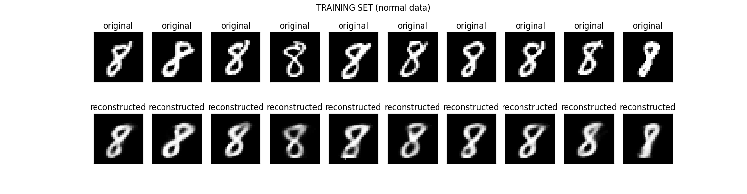
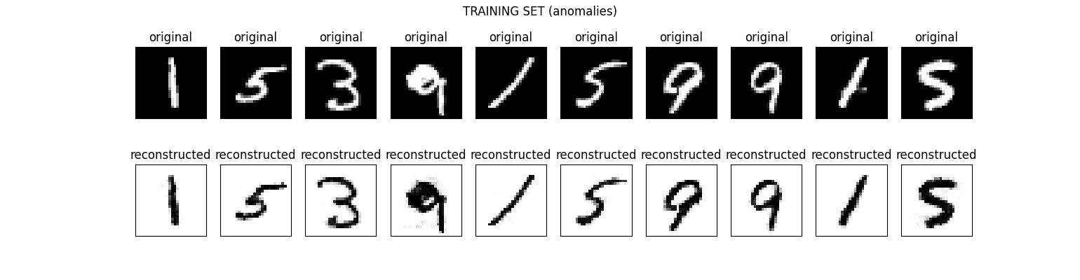
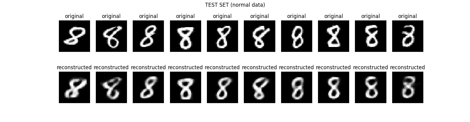
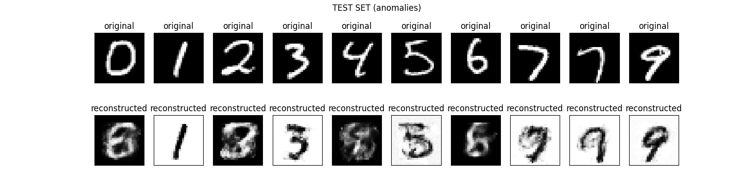
(a) AE–SAD.

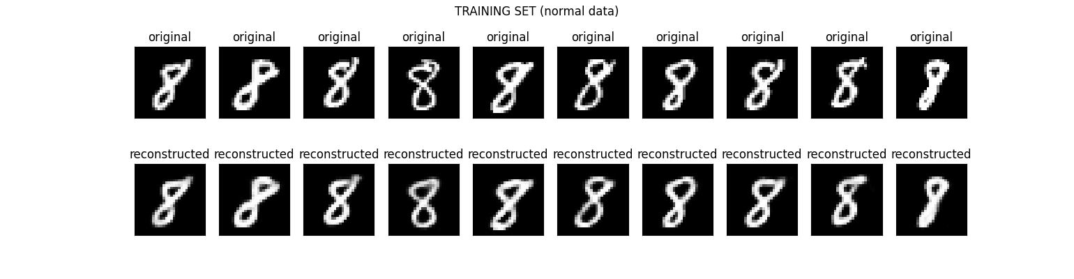
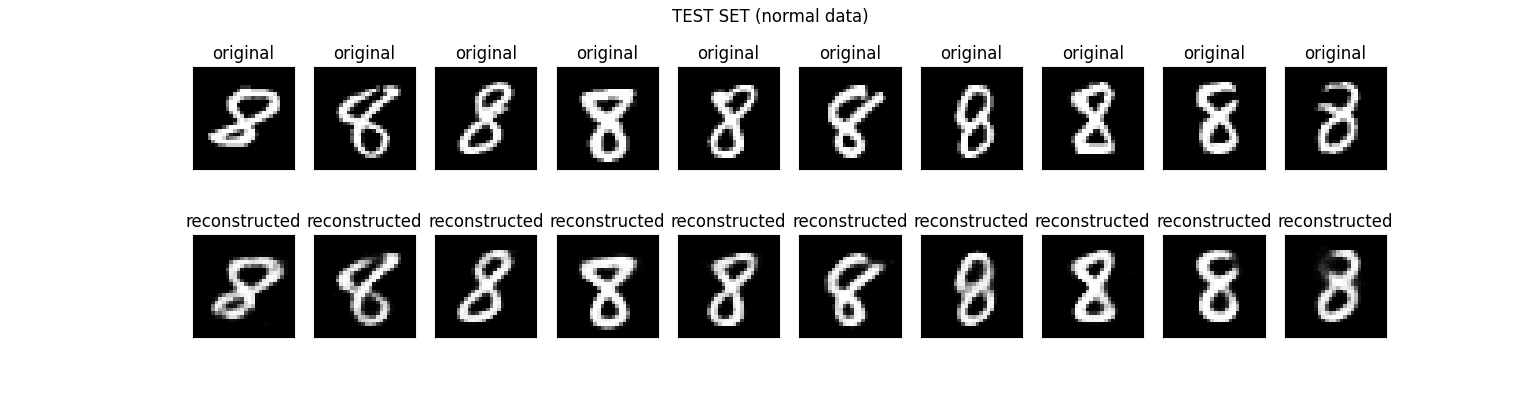
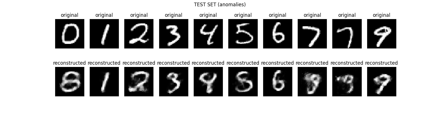
(b) Standard AE.

Figure 1: Original and reconstructed images of training and test set. In this example the class $8$ is normal and the class $1,3,5,9$ are the anomalous classes used in the training.

3.1 Comparative behavior with standard Autoencoder

In many real life situations, in general the anomalies that can arise in a evaluation phase may be generated from a distribution different from the anomalies used for the training.

In order to investigate the behaviour of our method in such a situation, we build a set-up in which, for each of the considered datasets, we select for the training phase all the items of a certain class as inliers, and a fixed number of examples from only some of the other classes as anomalies; the test set, on the contrary, is composed by all the classes of the selected dataset. In particular in the test set there will be

• examples from the normal class,

• anomalies belonging to classes that have been used for the training phase,

• anomalies belonging to classes that have not been used for the training, and thus are unknown for the model.

In Figure 1(a) are reported the original and the reconstructed images from the training and the test set obtained in a setting where the class $8$ of the dataset MNIST is considered as normal and the classes $1$, $3$, $5$, and $9$ are the anomalous classes used for the training. There are $100$ labeled anomalies in the training set. As we expected, in the training set the normal examples are well reconstructed in a similar way as what happens for the standard AE training setting, while the anomalies are reconstructed as the negative of the input images; for what concerns the test set we can see that the normal examples are again well reconstructed, while the anomalies must be distinguished in two different types: while the classes $1,3,5,9$, that have been used in the training, are reconstructed in a way very similar to the negative image, the remaining classes show a more confused reconstruction. In particular some unseen classes, such as $7$, are reconstructed in reverse because apparently the Autoencoder judges them more similar to the anomalies used for the training than to the normal class; other classes, such e.g. as $2$ and $4$, present a reconstruction more similar to the original image (the background remains black) but from which it is more difficult to determine the digit that it represents.

In any case all these reconstructions are very worse than the one obtained in a semi-supervised setting (Figure 1(b)), and this leads to better performances of the reconstruction error as anomaly score even in this setting where the Autoencoder is trained with only a portion of the anomalies.

Figure 2 reports some quantitative results associated with the above experiment. In particular, Figures 1(a) and (b) report the boxplot of the test reconstruction error associated with the examples of the classes $0$ to $9$ for the standard AE and for AE–SAD. These plots highlight the main effect of our strategy over the classical use of an AE, that is reconstruction errors of anomalous classes are greatly amplified (consider that the y-scale is logarithmic) and the overlapping with the normal class is reduced. For example, the class $1$, that is essentially indistinguishable from the normal data by the AE, is almost completely separated by our method. Clearly AE–SAD takes advantage of the fact that the class $1$ is an anomalous class seen during training. However, we can observe that a similar behavior is exhibited also by some classes that are not seen during training as, e.g., class $4$ and $7$. The reduced overlapping between reconstruction errors is witnessed by the comparison between AUCs (see 2(c)) which passes from $0.8775$ in the case of the AE to $0.9907$ after the adoption of the proposed strategy.

Class		AE	AE–SAD
seen	1	0.2780	0.9854	$+0.7074$
	3	0.9416	0.9960	$+0.0544$
	5	0.9365	0.9934	${+0.0569}$
	9	0.8863	0.9962	$+0.1099$
unseen	0	0.9907	0.9924	${+0.0017}$
	2	0.9718	0.9774	${+0.0056}$
	4	0.9431	0.9902	${+0.0471}$
	6	0.9527	0.9698	$+0.0171$
	7	0.9275	0.9919	${+0.0644}$

TABLE I: Comparison between the AUC of AE and AE–SAD on each anomalous class for the example of Figures 1 and 2.

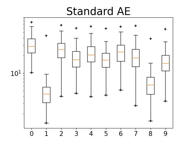
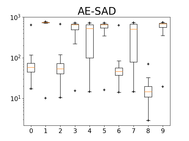
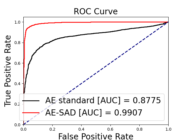
Figure 2: In this example the class $8$ is normal and the class $1,3,5,9$ are the anomalous classes used in the training.

Table I reports the AUC obtained on a test set consisting in unseen examples from the normal and each anomalous class of AE and AE–SAD, and the increase in AUC achieved by AE–SAD, respectively. Specifically, the first four rows concern classes seen during training, while the remaining five rows classes unseen during training. As a main result, we can observe that all the anomalous classes, both seen and unseen, take advantage of the AE–SAD strategy. As for the unseen classes, the increase in AUC is always above $+0.05$ and is practically close the maximum achievable, since all the final AUC values are around $0.99$. As for the unseen classes, two of them achieve sensible AUC improvements, namely class $4$ and $7$, while for the remaining classes there is a gain, even if less marked.

In conclusion, notably, all the seen anomalous classes, even those which are practically indistinguishable from the normal one by standard AE, become almost completely separated using our method. Moreover, also unseen anomalous may achieve large accuracy improvements either since they are reversely reconstructed or their associated reconstruction error get worse due to a more confused reconstruction.

4 Experimental results

In this section we describe experiments conducted to study the behavior of the proposed method. In particular, we start by describing the experimental settings (Section 4.1) and, subsequently, we report the experimental evaluation of AE–SAD driven by three main goals, namely

• studying how parameters affect its behavior,

• comparing its performance with existing algorithms,

• analyzing its effectiveness in the scenario of polluted data.

In detail, sections are organized as follows. In Sections 4.2 and 4.3 we describe the sensitivity of the method to the main parameters of the algorithm, namely the number of known anomalies, the regularization term and the number of training epochs. In Section 4.4 we compare AE–SAD with existing methods in the context where they are trained on a data set containing normal data and few known anomalies and tested on a data set with normal data and anomalies belonging to both seen and unseen anomalous classes. In Section 4.5 we test AE–SAD in the challenging scenario, often arising in real life applications, where the training set is polluted by mislabeled anomalies. Specifically, the methods are trained with a set containing normal data, data labeled as anomalous, and anomalous data incorrectly labeled as normal. Furthermore, we report, in Section 4.6, the behavior of the proposed technique when known anomalies belong to a set of classes.

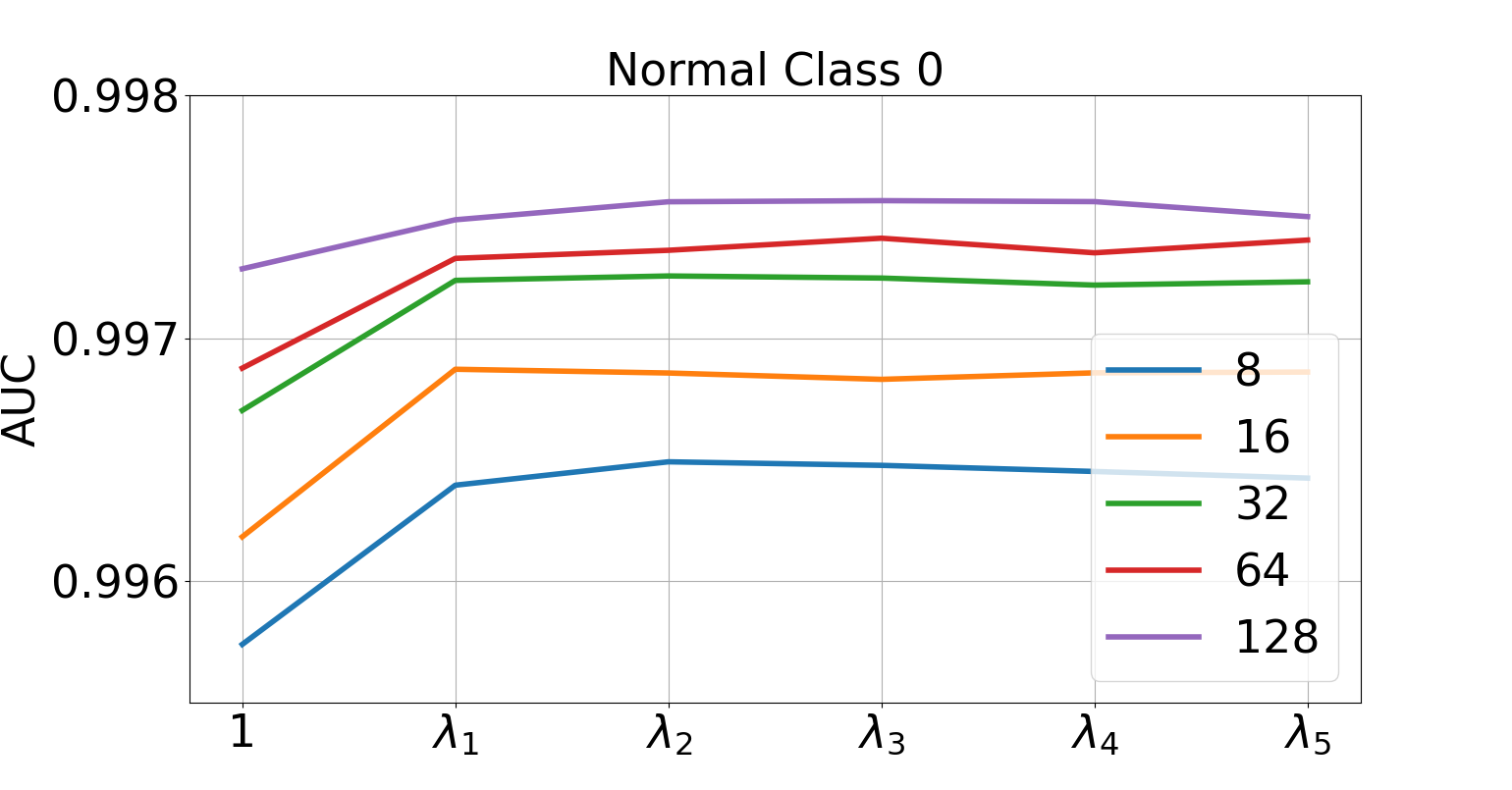
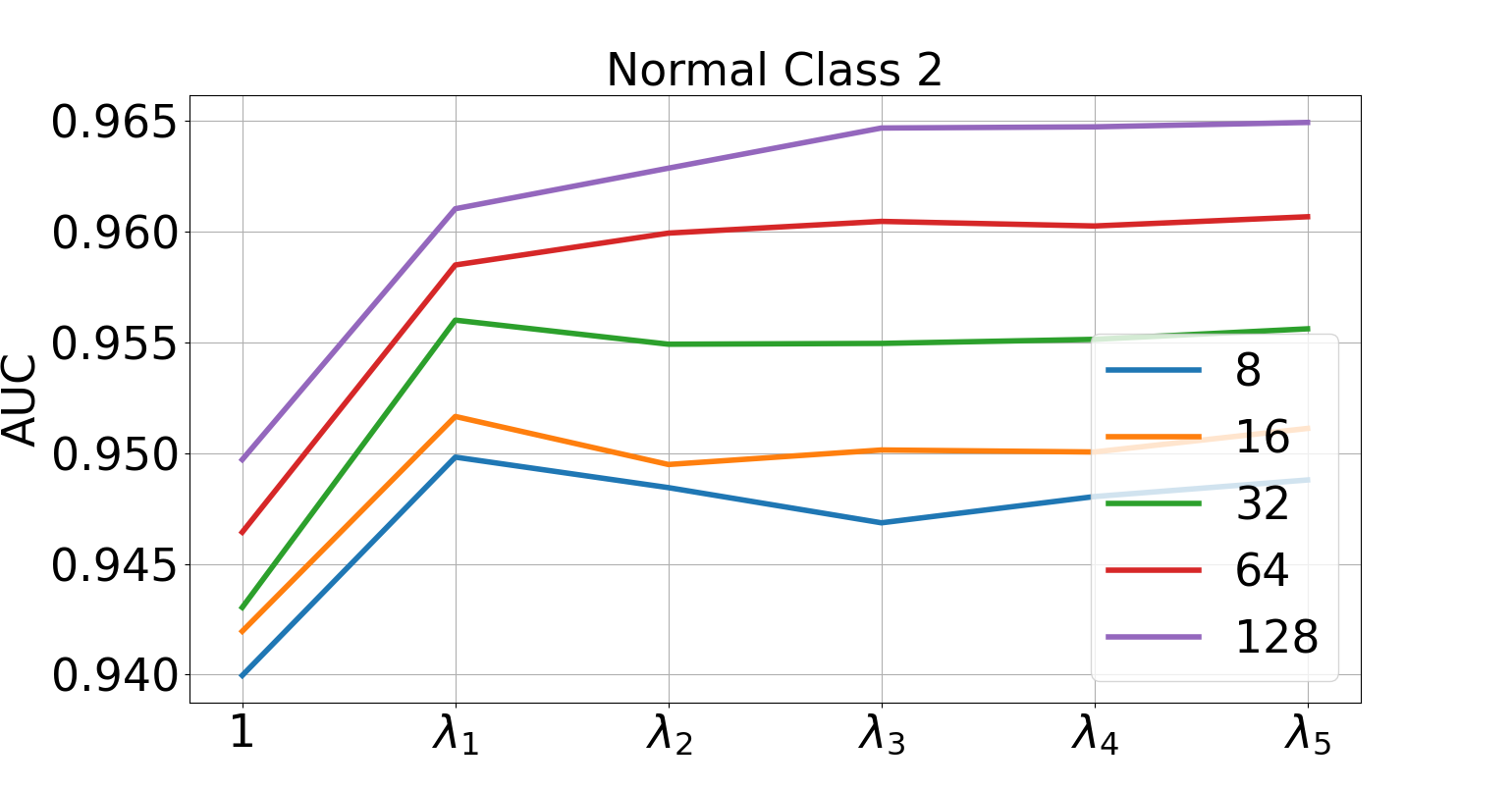
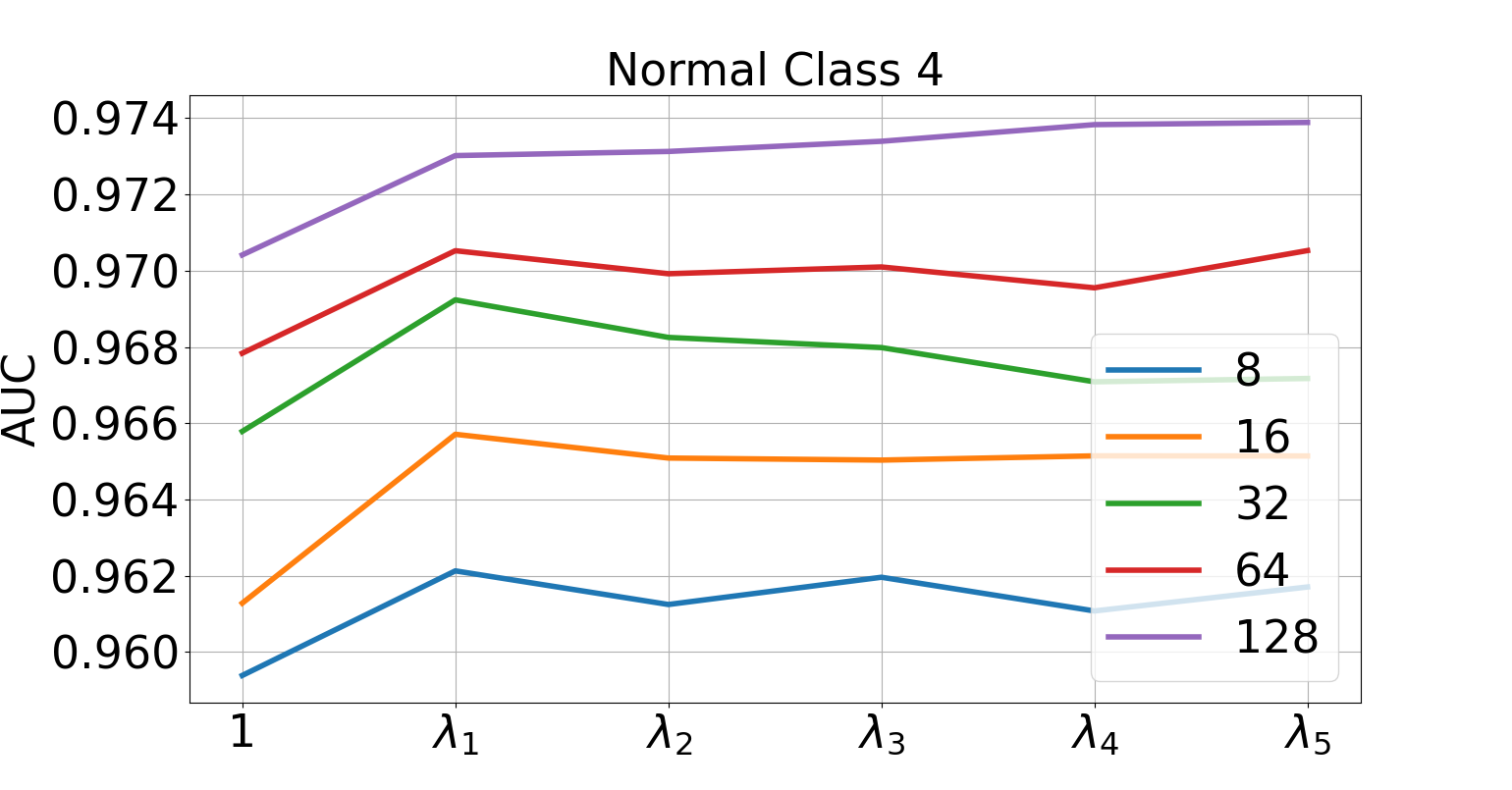
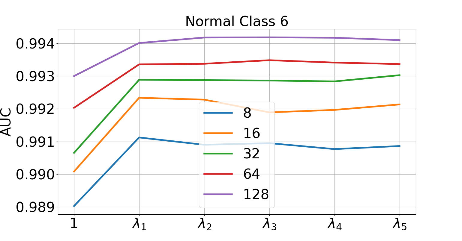
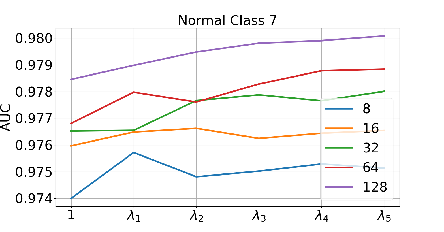
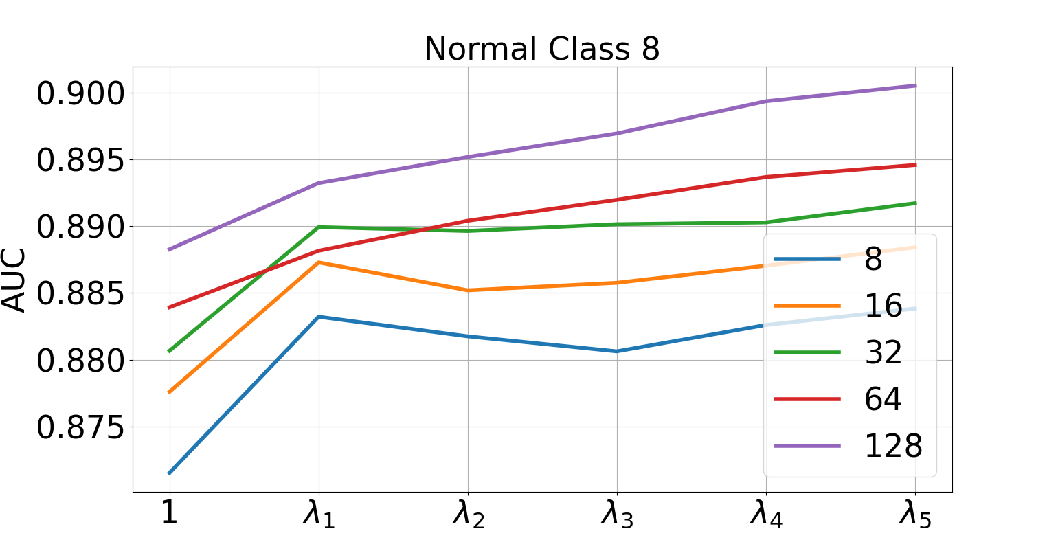
Figure 3: Sensitivity to the regularization parameter $\lambda$.

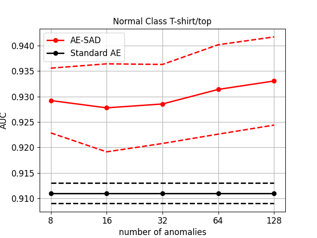
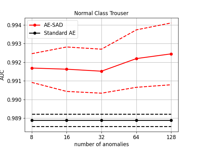
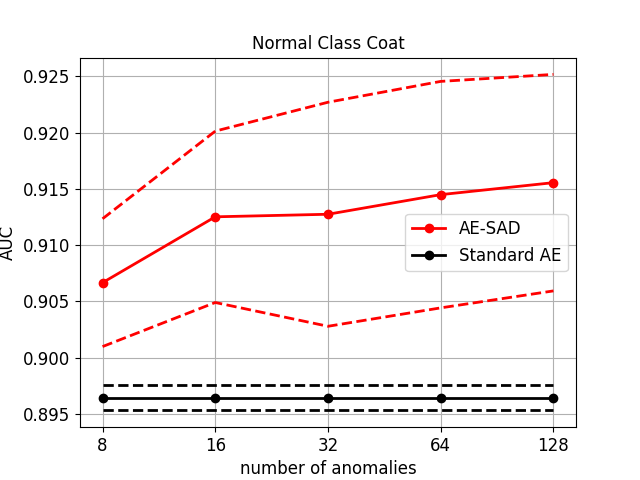
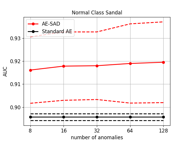
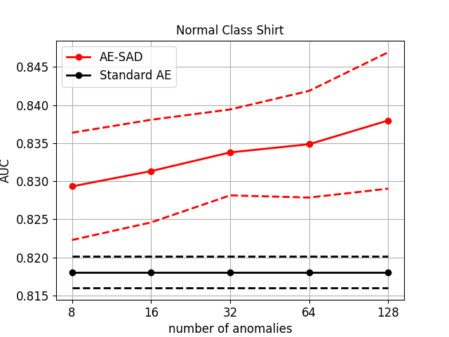
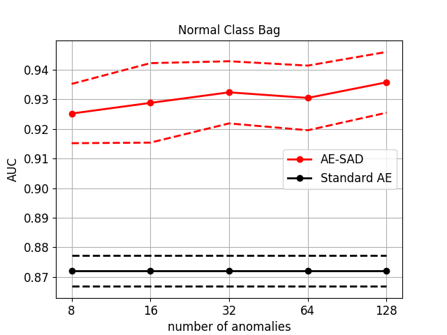
Figure 4: Sensitivity to the number of labeled anomalous examples $s$.

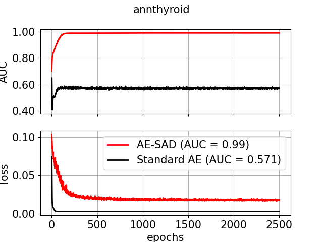
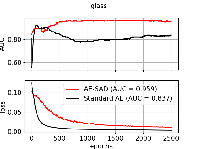
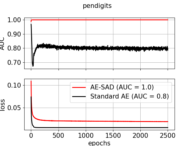
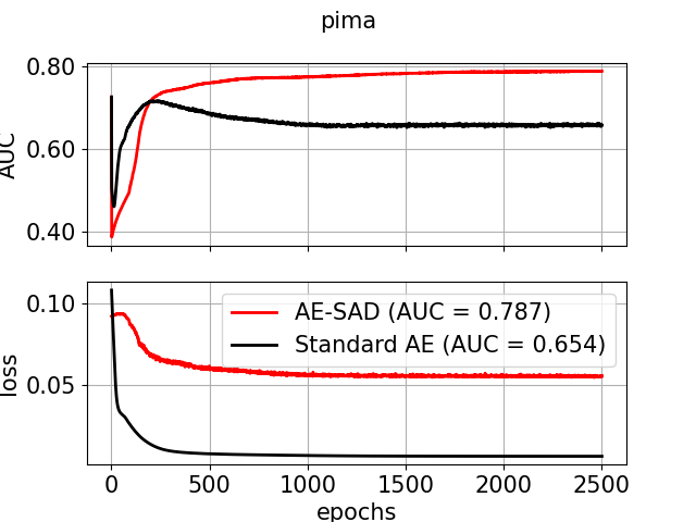
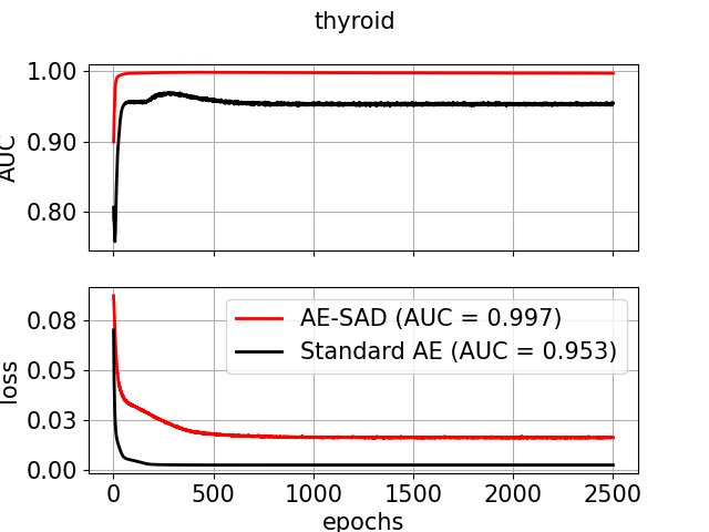
Figure 5: Sensitivity to the number of epochs. For both standard Autoencoder and AE–SAD is reported in the legend the AUC value relative to the epoch in which the lowest value of the loss has been observed.

4.1 Experimental settings

In general, given a multi-labeled dataset consisting of a training set and of a test set, we select some of the original classes to form the normal class of our problem and some other classes as known anomalous classes. The remaining classes form the unknown anomalous classes. Then, the training set for our method consists of all the training examples of the normal class, labeled as $0$, and of $s$ randomly picked training examples of the anomalies, labeled as $1$. Our test set coincides with the original test set and, hence, it comprises all the kinds of anomalies, both known and unknown.

In the rest of the section, we consider different rules for selecting normal and known anomalous classes in order to take into account different scenarios. We will refer to them later as one-vs-one, one-vs-many, one-vs-all, and many-vs-many, depending on the number of original classes used to form both the normal and the known anomalous classes. Moreover, sometimes we consider also the case in which the normal data is polluted by injecting a certain percentage of mislabeled known anomalous examples (these examples are wrongly labeled as $0$).

When an unsupervised method is employed to detect the anomalies in the test set, since it does not take advantage of the labels associated with training data, we remove the examples labeled as $1$ from the training set to avoid it incorporates them in the normal behavior. Indeed, in this case the method works as a semi supervised classifier and, hence, it expects to be trained only on normal data.

Because of fluctuations due to the random selection of the $s$ known anomalies, we run the methods on $10$ different versions of the same kind of training sets. Results of each experiment are obtained as the mean on the different runs.

The competitors considered were the baseline Autoencoder employing the same architecture of AE–SAD but with the classical reconstruction error loss, the One-Class SVM (OC-SVM) which is a classical statistical learning-based one-class classification approach [2], the $A^{3}$ method [27] which is deep learning semi-supervised anomaly detection approach exploiting the analysis of the activation values in its target network, and Deep-SAD [19] which is a deep learning semi-supervised anomaly detection approach extending the Deep-SVDD [18] strategy based on mapping normal data within an hyper-sphere. As for the datasets, depending on the experiment, we consider the tabular real-world anomaly detection specifc datasets belonging to the ODDS library [40], as well as the MNIST [29], E-MNIST [30], Fashion-MNIST [31], and CIFAR-10 [32] image datasets.

As for the architecture of AE–SAD, we employ an Autoencoder consisting of two layers for the encoder, a latent space of dimension $32$, and two layers symmetrical to the ones of the encoder for the decoder. We use dense layers on the MNIST and Fashion MNIST datasets and convolutional layers on CIFAR-10. As for the other methods, we employ the parameters suggested in their respective papers.

4.2 Sensitivity analysis to the parameters $\lambda$ and $s$

In this section, we intend to determine the impact of the regularization parameter $\lambda$ on the results of the method and the behavior for different numbers of labeled anomalies. To this aim, we first consider the MNIST dataset and vary both the number $s$ of labeled anomalies in $\{8,16,32,64,128\}$ and the value of the parameter $\lambda$.

As for the latter parameter, since it weights the contribution to the loss coming from the labeled anomalies, it makes sense to relate it to the number $s$ of anomalies seen during training. Thus, let $\alpha$ be a value in $[0,1]$. We denote by $\lambda(\alpha)$ the following value for the regularization parameter

$$\lambda(\alpha)=1+\alpha\left(\frac{n}{s}-1\right),$$

varying between $1$ (for $\alpha=0$) and $n/s$ (for $\alpha=1$). Since the weight of each is $1$ in our loss, for $\alpha=0$ each single anomalous example weights as a single inlier, while for $\alpha=1$ each single anomalous example weights as $n/s$ inliers and, thus, globally inliers and outliers contribute half of the total loss in terms of weights. For $\alpha>1$ outliers weight globally more than inliers. In our experiments, we varied $\lambda$ in $\lambda\in\{\lambda_{0}=\lambda(0)=1,\lambda_{1}=\lambda(\alpha_{1}),\dots,\lambda_{5}=\lambda(\alpha_{5})\}$, where $\alpha_{1},\ldots,\alpha_{5}$ are $5$ log-spaced values between $0.1$ and $2$.

As for the datasets, in this experiment we consider the one-vs-one setting. Consider a dataset containing $m$ classes. We fix in turn one of the $m$ classes as the normal one and then obtain $m-1$ different training sets by selecting one the remaining classes as the known anomalous. Since each of the considered datasets consists of $m=10$ classes and since for each training set we consider $10$ different versions, the total number of training sets is $10m(m-1)=900$.

Figure 3 reports the results of the experiment on MNIST. Since we consider $6$ different values for $\lambda$ and $5$ different values for $s$, the total number of runs is in this case $27,\!000$. Specifically each curve reports the average AUC of AE–SAD when the normal class is held fixed. All the curves show a similar behavior. As for the regularization parameter $\lambda$, it can be concluded that its selection does not represent a critical choice. For $\lambda>1$ some improvements can be appreciated, but the method appears to be not too much sensitive to the variation of the regularization parameter independently from the number of labeled anomalies. This behavior can be justified by the fact that, even if anomalies are few in comparison to normal examples and, moreover, even if anomalies would globally weight less than inliers in the loss function, the reconstruction error of a badly reconstructed anomaly (that is not reversely reconstructed as required by our loss) is potentially much larger than the reconstruction error associated with a single inlier. Indeed, if the network learned to output the original reconstruction of even a single anomaly, the associated loss contribution would be very large due to the requirement to minimize the distance to the target reverse reconstruction function. Informally, we can say that AE–SAD cannot afford to make a mistake in reconstructing anomalies. From the above analysis, as for the parameter $\lambda$ in the following, if not otherwise stated, we hold fixed $\lambda$ to the value $\lambda_{1}=\lambda(0.1)$.

Figure 4 shows the sensitivity to the parameter $s$ on Fashion-MNIST. The AUC of the baseline AE is also reported for comparison. The latter AUC is constant since AE in an unsupervised method and do not uses the labeled anomalies. These curves confirm the behavior already observed on MNIST. Summarizing, as for the number of labeled anomalies $s$, AE–SAD performs remarkably well even when only a few anomalies are available. The same reason provided above can be used to justify this additional result. As for the parameter $s$ in the following, if not otherwise stated, we set $s=8$ by default to considered the challenging scenario in which a limited number of labeled anomalous examples is available.

4.3 Sensitivity analysis to the number of epochs

The number training epochs is an important hyperparameter for all methods that employ neural networks.

In the anomaly detection context the choice of this hyperparameter might become critical since the value of the loss function of a standard AE is not indicative of the quality as anomaly detector. Indeed, while a low MSE value on the training set means that training examples are well reconstructed, this does not necessarily implies that anomalies are better identified. Differently, with our method we introduce a novel loss and a novel strategy to train an Autoencoder that aims at enlarging the difference between the reconstruction error of the anomalies and the ones of the normal items.

Thus in order to compare the behaviour of AE–SAD with standard Autoencoders as the number of epochs grows, we consider the ODDS datasets and we train both the models for $2500$ epochs and at each epoch we compute the AUC on the test set and the value of the relative loss function on the training set. Since the ODDS datasets are not partitioned into a training and a test set by design, we split each of them by randomly selecting the $60\%$ of the normal items to be part of the training set and keeping the rest for the test set. As for the anomalies, we randomly pick a number of them such that they represent the $5\%$ of the training set, while the remaining anomalies are used in the test set. For AE–SAD, we fix the parameter $\lambda$ by following the rule obtained in previous section.

The results reported in Figure 5 show that in general AE–SAD outperforms the standard AE in terms of AUC at each epoch. Moreover the trend of the AUC of our method is much more regular and almost always increasing. This can be justified because after a certain number of epochs the standard AE learns to reconstruct also the anomalies, while by using the loss (2) we always increase the contrast between the reconstruction of the two classes during all the training process. It can be concluded that, while the number of epochs is a critical hyperparameter for standard AE, this is not the case for AE–SAD. In our case it is not hard to select a good value for this hyperparameter, since the more epochs we consider, the higher the expected performances.

Legends of Figure 5 report between brackets the AUC value in the epoch in which the lowest value of the loss is reached. As we can see, while for AE–SAD a low value of the loss always implies an AUC value close to the maximum, the same fact does not hold for standard AE. Indeed, for what concerns the latter method, often the maximum AUC value is obtained when the value of the loss is still high. This happens because, the standard AE is able to generalize to classes not included in the training set that could share similarities with anomalies, while the same effect is mitigated in AE–SAD by the nature of the loss.

Finally from Figure 5, we can deduce that in general AE–SAD achieves good AUC values even after a relatively small number of epochs, thus the training is not too slow.

ODDS Datasets
Dataset ($d$)	AE–SAD	AE	OC-SVM	$A^{3}$	Deep-SAD
annthyroid ($6$)	.990$\pm$.001	.692$\pm$.104	.585$\pm$.003	.689$\pm$.084	.662$\pm$.040
arrhythmia ($274$)	.796$\pm$.054	.789$\pm$.011	.808$\pm$.019	.692$\pm$.041	.751$\pm$.036
breastw ($9$)	.992$\pm$.003	.995$\pm$.002	.994$\pm$.002	.995$\pm$.002	.977$\pm$.008
cardio ($21$)	.994$\pm$.002	.857$\pm$.078	.954$\pm$.003	.904$\pm$.025	.785$\pm$.071
glass ($9$)	.974$\pm$.014	.664$\pm$.114	.527$\pm$.182	.639$\pm$.098	.880$\pm$.076
ionosphere ($33$)	.971$\pm$.01	.910$\pm$.009	.918$\pm$.006	.668$\pm$.014	.953$\pm$.009
letter ($32$)	.908$\pm$.035	.802$\pm$.023	.546$\pm$.016	.539$\pm$.016	.768$\pm$.021
lympho ($18$)	.986$\pm$.011	.993$\pm$.007	.940$\pm$.043	.977$\pm$.037	.860$\pm$.158
mammography ($6$)	.916$\pm$.029	.874$\pm$.021	.880$\pm$.019	.835$\pm$.047	.759$\pm$.106
musk ($166$)	1.00$\pm$.000	1.00$\pm$.000	1.00$\pm$.000	1.00$\pm$.000	1.00$\pm$.000
optdigits ($64$)	1.00$\pm$.000	.975$\pm$.007	.718$\pm$.027	.906$\pm$.028	.843$\pm$.051
pendigits ($16$)	1.00$\pm$.000	.747$\pm$.083	.983$\pm$.006	.983$\pm$.009	.964$\pm$.023
pima ($8$)	.733$\pm$.022	.594$\pm$.033	.698$\pm$.013	.634$\pm$.049	.657$\pm$.024
satellite ($36$)	.907$\pm$.025	.812$\pm$.014	.728$\pm$.004	.802$\pm$.003	.827$\pm$.030
satimage-2 ($36$)	.999$\pm$.001	.998$\pm$.002	.997$\pm$.002	.982$\pm$.004	.968$\pm$.012
shuttle ($9$)	.808$\pm$.353	.914$\pm$.138	.993$\pm$.000	.977$\pm$.007	.984$\pm$.015
speech ($400$)	.479$\pm$.024	.463$\pm$.025	.465$\pm$.023	.535$\pm$.050	.478$\pm$.034
thyroid ($6$)	.987$\pm$.011	.922$\pm$.072	.897$\pm$.038	.776$\pm$.123	.885$\pm$.089
vertebral ($6$)	.635$\pm$.138	.444$\pm$.078	.522$\pm$.063	.351$\pm$.033	.558$\pm$.037
vowels ($12$)	.975$\pm$.021	.904$\pm$.026	.816$\pm$.051	.528$\pm$.061	.937$\pm$.055
wbc ($30$)	.970$\pm$.023	.964$\pm$.020	.953$\pm$.02	.878$\pm$.052	.891$\pm$.065
wine ($13$)	.994$\pm$.004	.829$\pm$.121	.998$\pm$.001	.893$\pm$.080	.817$\pm$.142

TABLE II: Comparison with competitors in the ODDS datasets.

MNIST
AE–SAD OC-SVM AE $A^{3}$ Deep-SAD mean AE–SAD — 1.00 0.91 1.00 0.85 0.94 OC-SVM 0.00 — 0.00 0.86 0.05 0.23 AE 0.09 1.00 — 1.00 0.70 0.70 $A^{3}$ 0.00 0.14 0.00 — 0.02 0.04 Deep-SAD 0.15 0.95 0.30 0.98 — 0.59 mean 0.06 0.74 0.28 0.94 0.38 —

Fashion MNIST
AE–SAD OC-SVM AE $A^{3}$ Deep-SAD mean AE–SAD — 1.00 0.98 0.98 0.64 0.90 OC-SVM 0.00 — 0.01 0.90 0.11 0.25 AE 0.02 0.99 — 0.97 0.38 0.59 $A^{3}$ 0.02 0.10 0.03 — 0.03 0.05 Deep-SAD 0.36 0.89 0.62 0.97 — 0.51 mean 0.11 0.65 0.37 0.89 0.26 —

CIFAR-10
AE–SAD OC-SVM AE $A^{3}$ Deep-SAD mean AE–SAD — 0.97 1.00 0.86 0.81 0.91 OC-SVM 0.03 — 0.48 0.39 0.29 0.30 AE 0.00 0.52 — 0.54 0.42 0.37 $A^{3}$ 0.14 0.61 0.46 — 0.48 0.42 Deep-SAD 0.19 0.71 0.58 0.52 — 0.50 mean 0.09 0.70 0.63 0.48 0.50 —

TABLE III: Probability of winning for each pair of methods in the one-vs-one experimental setting.

MNIST
0 1 2 3 4 5 6 7 8 9 $\mu$ 0  $-$ 1.00 1.00 1.00 0.98 1.00 1.00 0.95 1.00 0.98 0.99 1 0.98  $-$ 0.90 0.95 1.00 0.98 0.95 1.00 0.95 1.00 0.97 2 0.92 1.00  $-$ 0.95 0.92 0.98 0.88 0.95 1.00 0.92 0.95 3 0.90 1.00 0.95  $-$ 0.90 0.95 1.00 0.98 1.00 0.98 0.96 4 0.82 0.98 1.00 1.00  $-$ 0.88 0.70 0.95 0.98 0.88 0.91 5 0.88 1.00 0.98 1.00 0.92  $-$ 0.98 1.00 1.00 1.00 0.97 6 0.85 1.00 0.95 0.98 0.88 0.95  $-$ 0.90 1.00 1.00 0.94 7 0.95 1.00 0.95 0.98 0.98 1.00 0.98  $-$ 0.98 1.00 0.98 8 0.72 0.98 0.80 0.75 0.75 0.78 0.75 0.72  $-$ 0.80 0.78 9 0.88 1.00 1.00 0.98 0.95 0.98 0.92 1.00 0.92  $-$ 0.96 $\mu$ 0.88 0.99 0.95 0.95 0.92 0.94 0.91 0.94 0.98 0.95 0.94

Fashion MNIST
0 1 2 3 4 5 6 7 8 9 $\mu$ 0  $-$ 0.95 0.98 0.92 0.95 0.95 0.98 0.85 0.90 0.85 0.92 1 1.00  $-$ 1.00 0.98 1.00 0.98 1.00 1.00 1.00 0.95 0.99 2 1.00 0.88  $-$ 0.98 0.88 0.95 0.95 0.90 0.88 0.92 0.92 3 0.95 0.98 0.92  $-$ 0.90 0.92 0.95 0.88 0.92 0.82 0.92 4 0.98 1.00 0.85 1.00  $-$ 0.90 0.90 0.78 0.82 0.80 0.89 5 0.88 0.80 0.88 0.92 0.80  $-$ 0.80 1.00 0.82 0.92 0.87 6 0.98 0.98 0.88 1.00 0.95 1.00  $-$ 0.95 1.00 0.98 0.97 7 0.98 0.90 0.92 0.92 0.98 1.00 0.98  $-$ 0.92 0.98 0.95 8 0.82 0.75 0.85 0.80 0.82 0.80 0.78 0.82  $-$ 0.80 0.81 9 0.68 0.82 0.62 0.72 0.72 0.72 0.85 0.98 0.75  $-$ 0.76 $\mu$ 0.92 0.89 0.88 0.92 0.89 0.91 0.91 0.91 0.89 0.89 0.90
CIFAR-10
0 1 2 3 4 5 6 7 8 9 $\mu$ 0  $-$ 1.00 1.00 1.00 0.88 1.00 1.00 1.00 1.00 1.00 0.99 1 0.92  $-$ 1.00 0.52 1.00 1.00 0.72 1.00 1.00 0.78 0.88 2 1.00 1.00  $-$ 1.00 1.00 1.00 0.98 0.95 1.00 1.00 0.99 3 1.00 1.00 1.00  $-$ 1.00 1.00 1.00 1.00 1.00 1.00 1.00 4 0.98 1.00 0.78 1.00  $-$ 0.88 1.00 0.92 1.00 0.85 0.93 5 0.98 1.00 1.00 0.98 1.00  $-$ 1.00 1.00 1.00 1.00 0.99 6 0.98 0.75 0.95 0.85 1.00 0.88  $-$ 1.00 0.78 0.85 0.89 7 0.98 0.90 0.82 1.00 0.70 0.80 0.70  $-$ 1.00 0.65 0.84 8 0.95 1.00 1.00 0.95 1.00 1.00 1.00 1.00  $-$ 1.00 0.99 9 0.70 0.78 0.70 0.48 0.55 0.40 0.70 0.48 0.45  $-$ 0.58 $\mu$ 0.94 0.94 0.92 0.86 0.90 0.88 0.90 0.93 0.91 0.90 0.91

TABLE IV: Probability of winning of AE–SAD for each pair of normal and anomalous classes in the one-vs-one setting.

4.4 Comparison with other methods

In this section, we compare AE–SAD with the baseline AE, OC-SVM, $A^{3}$, and Deep-SAD. First, we test them on the ODDS datasets splitting them into training and test set in the same way as previous section. Since the selection of both anomalies and normal examples for training and test set is done by random sampling, we tested all the considered methods on 5 different runs for each dataset and we compute the mean and the standard deviation of the AUC. The results, reported in the Table II show that our method almost always achieves better performances than competitors, and sometimes this improvements are relevant.

We also consider for the comparison with the competitors the MNIST, Fashion-MNIST and CIFAR-10 datasets, for which we implement the one-vs-one setting already illustrated in Section 4.2. This setting simulates the scenario in which the detector has limited knowledge of the expected anomalies and, as such, it is a notable scenarios to deal with.

Table III reports the relative number of wins for each pair of methods on the MNIST, Fashion MNIST, and CIFAR-10 datasets. Specifically, each entry of the table is the probability that the method located on the corresponding row scores an AUC greater than that of the method located on the corresponding column. In the considered setting AE–SAD shows a larger probability of winning over all the competitors on all the datasets. Deep-SAD is the runner-up in terms of number of wins, while $A^{3}$ does not perform sufficiently in this setting despite being a semi-supervised method. In Section 4.6, we compare AE–SAD and $A^{3}$ on a setting where competitor performance are shown in [27] to be strong across various configurations.

Table IV details the result for each pair of normal and known anomalous classes, by reporting the relative number of wins of AE–SAD on the competitors. Specifically, each entry of the table is the probability that the AUC scored by AE–SAD is greater than the AUC scored by another method. For almost all the combinations AE–SAD is preferable to a randomly selected method of the pool.

To provide details also on the comparison of the methods on the each single dataset, Figure 7 reports the scatter plot of the AUC of AE–SAD (on the $y$-axis) vs the AUC of each competitor (on the $x$-axis) associated with each of the above experiments. Specifically, blue $+$-marks are relative to the experiments described in this section, while red $\times$-marks are relative experiments reported in the next section concerning polluted normal data. The plots provide a more complete picture of the relative performances of our method.

4.5 Normal data polluted

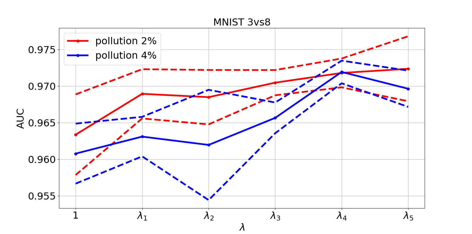
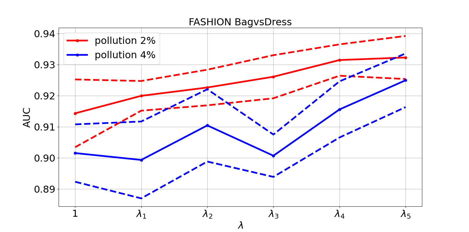
Figure 6: Sensitivity analysis of the regularization parameter $\lambda$ for different levels of pollution.

MNIST 3vs[4,5,6]
Method	Pollution
	$0.25\%$	$0.5\%$	$2.5\%$	$5\%$	$12.5\%$
AE–SAD	.968$\pm$.007	.966$\pm$.003	.957$\pm$.007	.961$\pm$.009	.955$\pm$.003
Standard AE	.944$\pm$.005	.942$\pm$.004	.919$\pm$.006	.904$\pm$.005	.864$\pm$.011
OC-SVM	.871$\pm$.000	.870$\pm$.000	.863$\pm$.000	.854$\pm$.000	.821$\pm$.001
$A^{3}$	.622$\pm$.037	.675$\pm$.035	.725$\pm$.099	.653$\pm$.085	.603$\pm$.077
Deep-SAD	.958$\pm$.009	.957$\pm$.004	.948$\pm$.003	.944$\pm$.009	.911$\pm$.032
Fashion MNIST 3vs[7,8,9]
Method	Pollution
	$0.25\%$	$0.5\%$	$2.5\%$	$5\%$	$12.5\%$
AE–SAD	.946$\pm$.002	.944$\pm$.003	.945$\pm$.004	.942$\pm$.004	.939$\pm$.002
Standard AE	.917$\pm$.001	.908$\pm$.002	.890$\pm$.003	.880$\pm$.003	.858$\pm$.002
OC-SVM	.902$\pm$.000	.901$\pm$.000	.898$\pm$.000	.895$\pm$.000	.880$\pm$.000
$A^{3}$	.877$\pm$.008	.875$\pm$.005	.861$\pm$.013	.852$\pm$.013	.838$\pm$.015
Deep-SAD	.925$\pm$.015	.913$\pm$.005	.904$\pm$.016	.905$\pm$.013	.901$\pm$.009

TABLE V: Comparison with competitors for various percentage levels of pollution.

MNIST
Class	AE–SAD	AE	OC-SVM	$A^{3}$	Deep-SAD
0	.980$\pm$.006	.885$\pm$.015	.911$\pm$.001	.770$\pm$.018	.910$\pm$.037
1	.996$\pm$.001	.996$\pm$.001	.986$\pm$.001	.983$\pm$.038	.983$\pm$.011
2	.913$\pm$.020	.767$\pm$.024	.729$\pm$.002	.676$\pm$.018	.869$\pm$.033
3	.929$\pm$.015	.821$\pm$.010	.820$\pm$.001	.730$\pm$.013	.861$\pm$.045
4	.940$\pm$.009	.854$\pm$.013	.876$\pm$.001	.794$\pm$.066	.880$\pm$.044
5	.915$\pm$.014	.807$\pm$.017	.697$\pm$.002	.484$\pm$.110	.827$\pm$.058
6	.958$\pm$.012	.877$\pm$.023	.863$\pm$.001	.882$\pm$.083	.925$\pm$.033
7	.956$\pm$.023	.907$\pm$.005	.895$\pm$.001	.879$\pm$.057	.900$\pm$.031
8	.843$\pm$.018	.750$\pm$.016	.788$\pm$.001	.663$\pm$.069	.866$\pm$.028
9	.942$\pm$.016	.897$\pm$.008	.884$\pm$.001	.829$\pm$.066	.922$\pm$.010
Fashion MNIST
Class	AE–SAD	AE	OC-SVM	$A^{3}$	Deep-SAD
T-shirt/top	.911$\pm$.071	.781$\pm$.007	.859$\pm$.001	.692$\pm$.053	.831$\pm$.061
Trouser	.980$\pm$.008	.958$\pm$.003	.957$\pm$.001	.949$\pm$.009	.957$\pm$.026
Pullover	.877$\pm$.039	.729$\pm$.016	.843$\pm$.001	.576$\pm$.103	.801$\pm$.072
Dress	.920$\pm$.028	.807$\pm$.009	.879$\pm$.001	.857$\pm$.024	.904$\pm$.021
Coat	.847$\pm$.041	.770$\pm$.039	.853$\pm$.001	.762$\pm$.064	.843$\pm$.049
Sandal	.908$\pm$.018	.633$\pm$.025	.807$\pm$.001	.841$\pm$.037	.864$\pm$.015
Shirt	.796$\pm$.037	.701$\pm$.039	.778$\pm$.001	.452$\pm$.078	.760$\pm$.030
Sneaker	.982$\pm$.004	.927$\pm$.010	.975$\pm$.001	.970$\pm$.004	.931$\pm$.058
Bag	.940$\pm$.019	.541$\pm$.009	.755$\pm$.001	.607$\pm$.051	.878$\pm$.052
Ankle boot	.971$\pm$.012	.807$\pm$.023	.952$\pm$.001	.966$\pm$.018	.937$\pm$.068

TABLE VI: Comparison with competitors in the one-vs-all polluted setting.

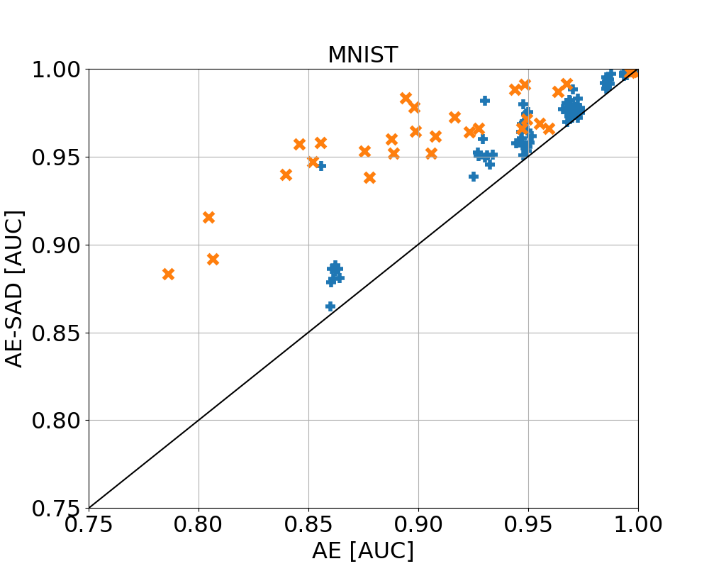
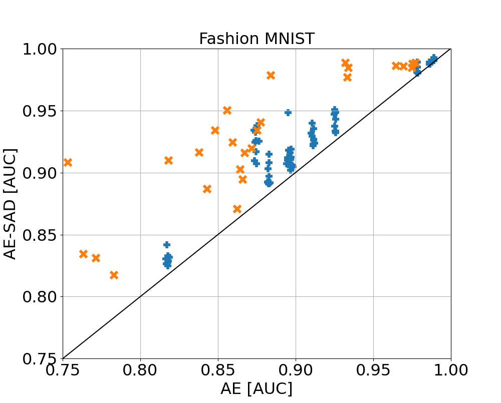
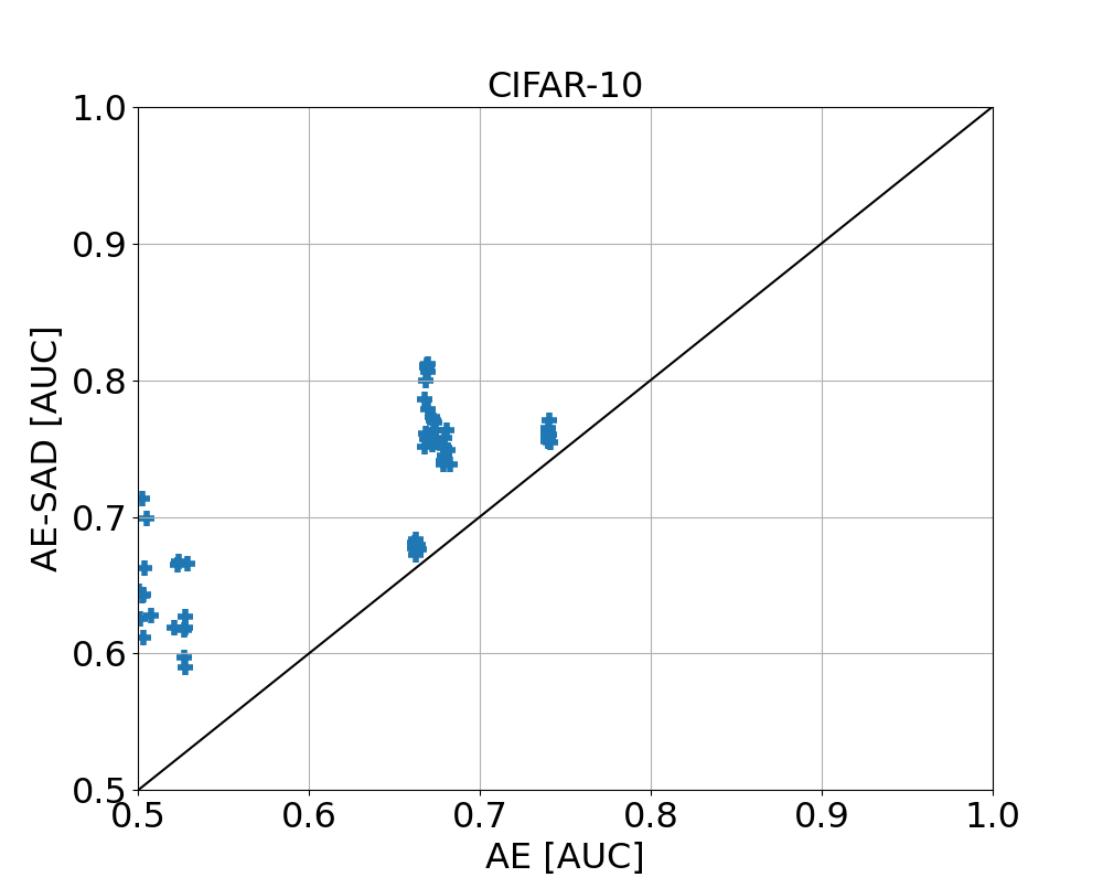
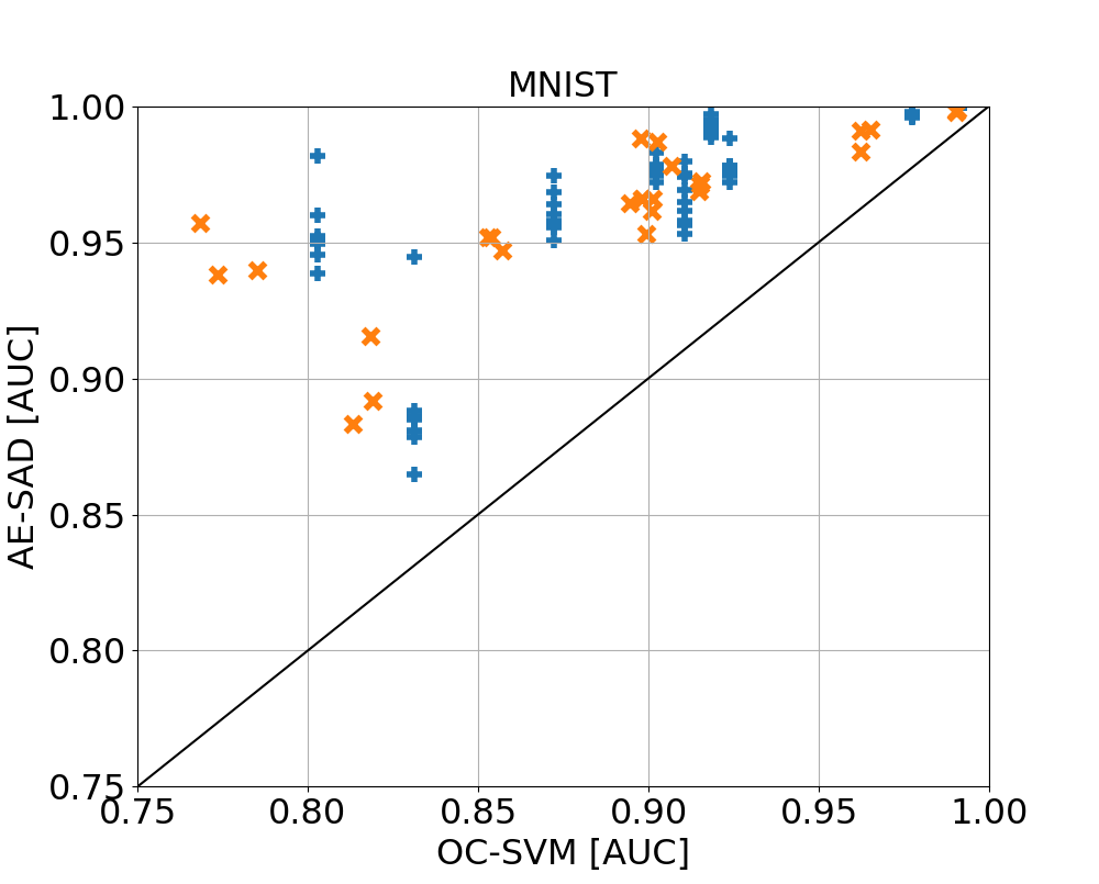
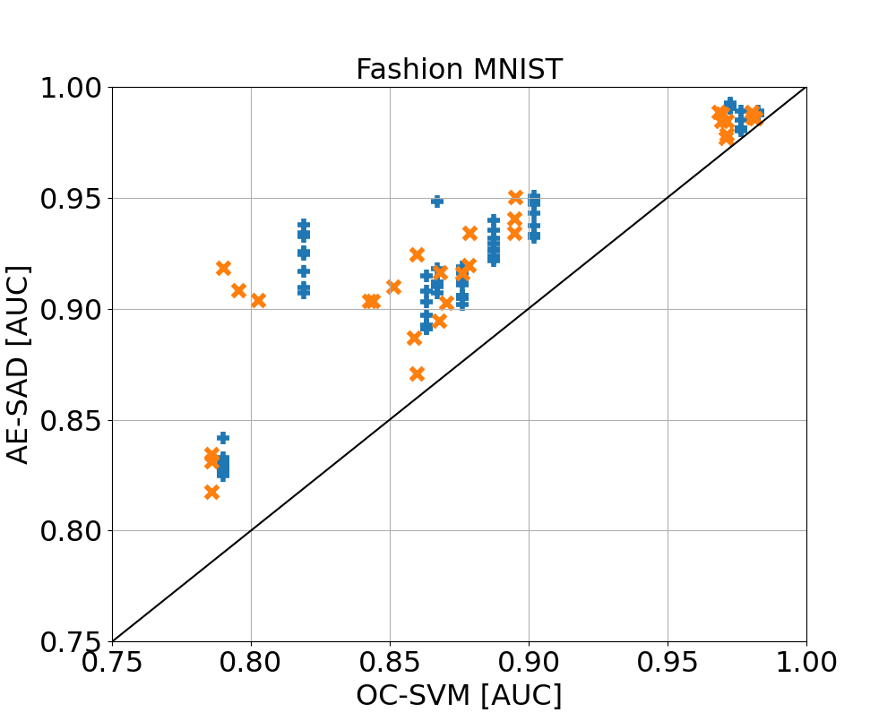
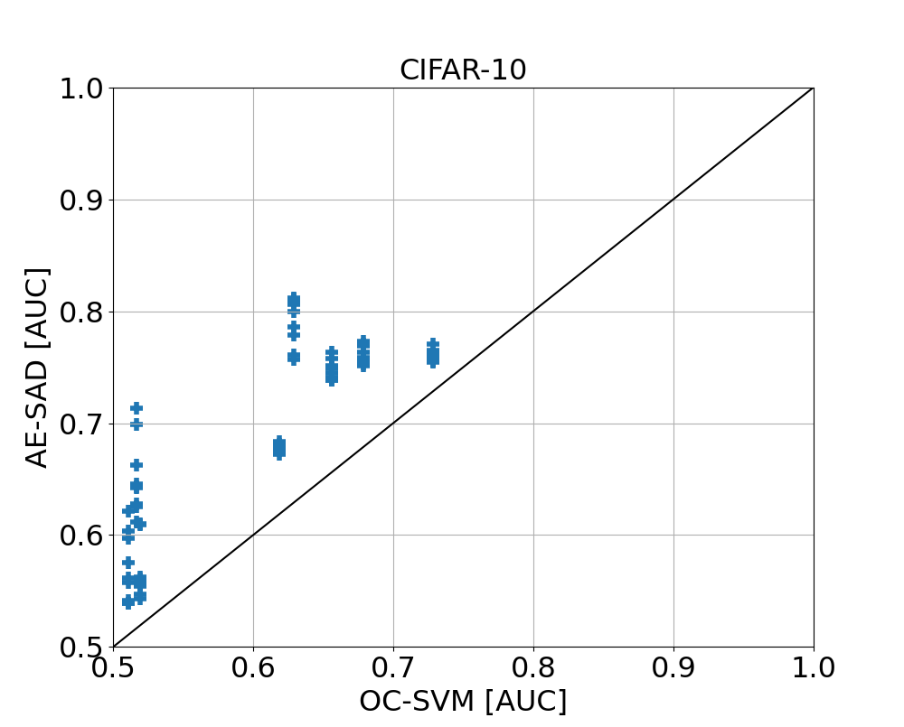
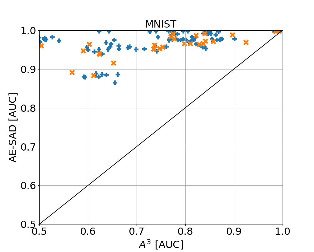
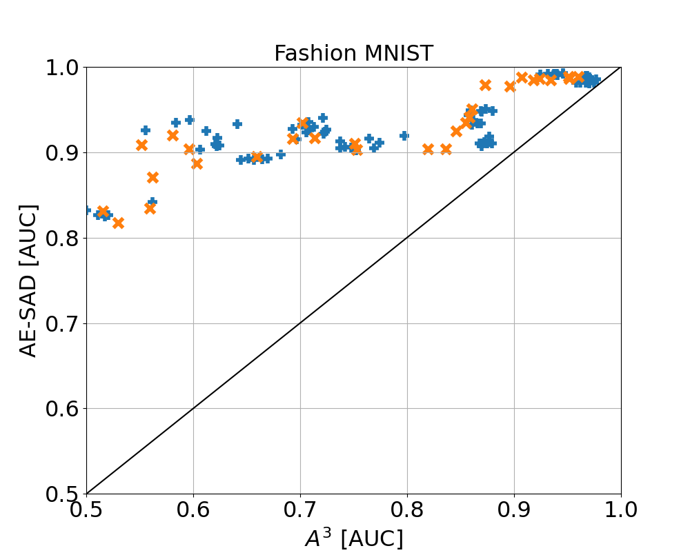
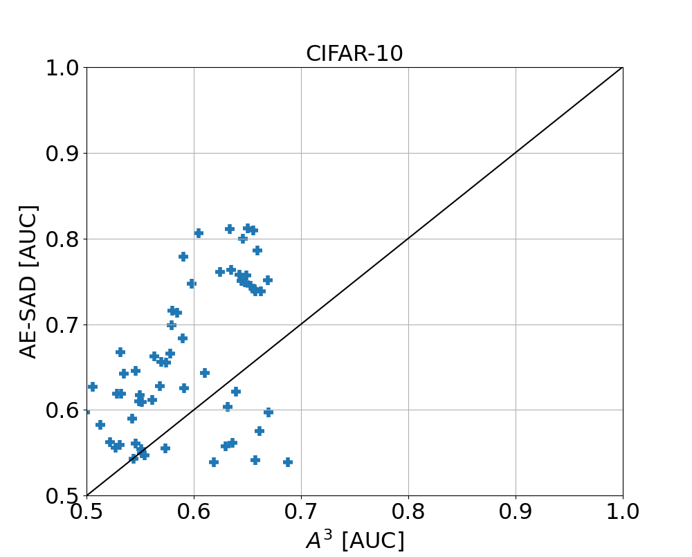
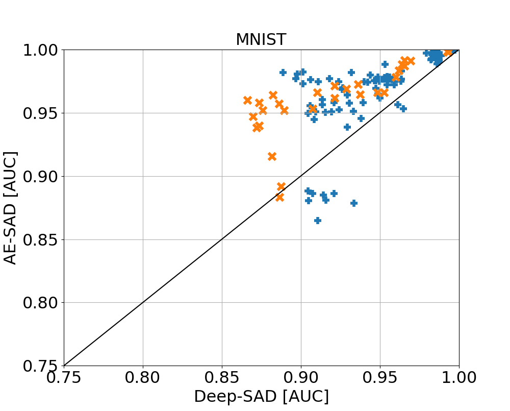
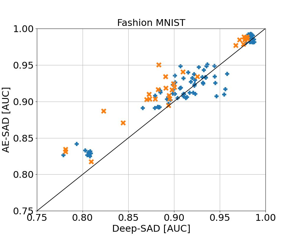
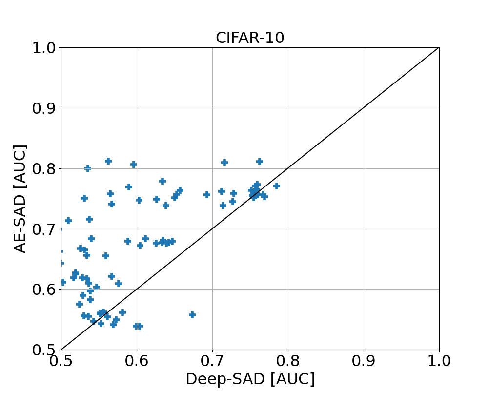
Figure 7: Comparison of the AUCs of AE–SAD and competitors on both clean (blue $+$-marks) and polluted (red $\times$-marks) data.

Dataset		MNIST					Fashion MNIST
N	A	AE–SAD	AE	OC-SVM	$A^{3}$	Deep-SAD	AE–SAD	AE	OC-SVM	$A^{3}$	Deep-SAD
0	[1,2,3]	.983$\pm$.007	.896$\pm$.005	.962$\pm$.000	.770$\pm$.083	.962$\pm$.015	.934$\pm$.003	.849$\pm$.002	.879$\pm$.000	.702$\pm$.042	.891$\pm$.020
	[4,5,6]	.991$\pm$.001	.968$\pm$.004	.965$\pm$.000	.840$\pm$.085	.965$\pm$.006	.920$\pm$.004	.870$\pm$.003	.878$\pm$.000	.581$\pm$.049	.900$\pm$.003
	[7,8,9]	.991$\pm$.001	.948$\pm$.005	.962$\pm$.000	.775$\pm$.061	.969$\pm$.005	.916$\pm$.002	.867$\pm$.002	.876$\pm$.000	.693$\pm$.012	.898$\pm$.006
1	[0,2,3]	.998$\pm$.000	.998$\pm$.000	.991$\pm$.000	.986$\pm$.007	.993$\pm$.003	.988$\pm$.002	.975$\pm$.001	.970$\pm$.000	.907$\pm$.043	.978$\pm$.003
	[4,5,6]	.998$\pm$.000	.997$\pm$.000	.990$\pm$.000	.992$\pm$.003	.993$\pm$.002	.984$\pm$.001	.974$\pm$.001	.969$\pm$.000	.934$\pm$.008	.977$\pm$.003
	[7,8,9]	.998$\pm$.000	.996$\pm$.000	.990$\pm$.000	.985$\pm$.019	.993$\pm$.002	.988$\pm$.000	.978$\pm$.001	.968$\pm$.000	.951$\pm$.006	.980$\pm$.003
2	[0,1,3]	.940$\pm$.013	.841$\pm$.003	.785$\pm$.001	.623$\pm$.089	.873$\pm$.013	.910$\pm$.002	.861$\pm$.003	.851$\pm$.000	.751$\pm$.023	.873$\pm$.015
	[4,5,6]	.938$\pm$.004	.879$\pm$.008	.774$\pm$.001	.624$\pm$.086	.872$\pm$.028	.871$\pm$.010	.819$\pm$.002	.860$\pm$.000	.562$\pm$.038	.844$\pm$.020
	[7,8,9]	.957$\pm$.007	.844$\pm$.008	.768$\pm$.001	.753$\pm$.102	.886$\pm$.024	.887$\pm$.002	.844$\pm$.003	.859$\pm$.000	.603$\pm$.021	.823$\pm$.045
3	[0,1,2]	.947$\pm$.002	.851$\pm$.002	.857$\pm$.000	.591$\pm$.071	.869$\pm$.049	.950$\pm$.004	.855$\pm$.002	.895$\pm$.000	.861$\pm$.015	.883$\pm$.067
	[4,5,6]	.952$\pm$.004	.905$\pm$.006	.854$\pm$.000	.736$\pm$.049	.889$\pm$.021	.934$\pm$.004	.876$\pm$.003	.895$\pm$.000	.855$\pm$.015	.909$\pm$.009
	[7,8,9]	.952$\pm$.008	.891$\pm$.010	.853$\pm$.000	.735$\pm$.042	.876$\pm$.038	.941$\pm$.001	.879$\pm$.004	.895$\pm$.000	.858$\pm$.013	.926$\pm$.023
4	[0,1,2]	.953$\pm$.014	.875$\pm$.003	.899$\pm$.000	.747$\pm$.055	.907$\pm$.009	.916$\pm$.004	.837$\pm$.003	.868$\pm$.000	.714$\pm$.051	.882$\pm$.009
	[3,5,6]	.966$\pm$.005	.926$\pm$.004	.901$\pm$.000	.798$\pm$.067	.910$\pm$.022	.895$\pm$.008	.865$\pm$.003	.868$\pm$.000	.660$\pm$.046	.870$\pm$.008
	[7,8,9]	.961$\pm$.007	.906$\pm$.004	.901$\pm$.000	.737$\pm$.063	.921$\pm$.026	.903$\pm$.004	.864$\pm$.002	.870$\pm$.000	.753$\pm$.016	.894$\pm$.027
5	[0,1,2]	.958$\pm$.006	.856$\pm$.004	.731$\pm$.001	.482$\pm$.092	.873$\pm$.006	.903$\pm$.004	.715$\pm$.008	.844$\pm$.000	.836$\pm$.015	.873$\pm$.014
	[3,4,6]	.964$\pm$.003	.916$\pm$.008	.725$\pm$.001	.603$\pm$.045	.882$\pm$.021	.903$\pm$.005	.746$\pm$.005	.843$\pm$.001	.819$\pm$.027	.879$\pm$.013
	[7,8,9]	.960$\pm$.005	.889$\pm$.005	.722$\pm$.001	.504$\pm$.048	.866$\pm$.014	.925$\pm$.007	.858$\pm$.005	.860$\pm$.000	.846$\pm$.048	.899$\pm$.014
6	[0,1,2]	.978$\pm$.003	.899$\pm$.002	.907$\pm$.000	.777$\pm$.098	.960$\pm$.011	.831$\pm$.007	.771$\pm$.003	.786$\pm$.000	.516$\pm$.033	.781$\pm$.041
	[3,4,5]	.987$\pm$.002	.962$\pm$.003	.903$\pm$.001	.822$\pm$.088	.965$\pm$.007	.818$\pm$.008	.783$\pm$.003	.786$\pm$.000	.530$\pm$.039	.781$\pm$.009
	[7,8,9]	.988$\pm$.002	.943$\pm$.005	.898$\pm$.000	.897$\pm$.048	.963$\pm$.005	.834$\pm$.002	.763$\pm$.002	.786$\pm$.000	.560$\pm$.027	.809$\pm$.009
7	[0,1,2]	.972$\pm$.001	.916$\pm$.002	.916$\pm$.000	.841$\pm$.046	.936$\pm$.012	.989$\pm$.001	.934$\pm$.007	.980$\pm$.000	.960$\pm$.009	.977$\pm$.002
	[3,4,5]	.969$\pm$.002	.956$\pm$.002	.915$\pm$.000	.924$\pm$.022	.929$\pm$.010	.986$\pm$.001	.966$\pm$.002	.981$\pm$.000	.924$\pm$.031	.978$\pm$.003
	[6,8,9]	.971$\pm$.003	.949$\pm$.003	.915$\pm$.000	.857$\pm$.048	.921$\pm$.016	.986$\pm$.001	.970$\pm$.003	.981$\pm$.000	.951$\pm$.023	.980$\pm$.003
8	[0,1,2]	.915$\pm$.007	.804$\pm$.009	.819$\pm$.001	.652$\pm$.042	.882$\pm$.025	.918$\pm$.004	.701$\pm$.007	.790$\pm$.000	.490$\pm$.055	.891$\pm$.030
	[3,4,5]	.892$\pm$.009	.802$\pm$.010	.819$\pm$.001	.567$\pm$.084	.887$\pm$.024	.908$\pm$.020	.753$\pm$.006	.795$\pm$.000	.552$\pm$.057	.895$\pm$.024
	[6,7,9]	.883$\pm$.011	.782$\pm$.010	.813$\pm$.000	.612$\pm$.944	.886$\pm$.015	.904$\pm$.017	.737$\pm$.005	.803$\pm$.001	.596$\pm$.024	.895$\pm$.023
9	[0,1,2]	.964$\pm$.001	.899$\pm$.002	.895$\pm$.000	.829$\pm$.028	.937$\pm$.006	.978$\pm$.002	.886$\pm$.007	.971$\pm$.000	.873$\pm$.050	.972$\pm$.006
	[3,4,5]	.966$\pm$.002	.959$\pm$.001	.898$\pm$.000	.837$\pm$.031	.953$\pm$.011	.977$\pm$.003	.934$\pm$.003	.971$\pm$.000	.896$\pm$.033	.967$\pm$.014
	[6,7,8]	.966$\pm$.004	.948$\pm$.002	.898$\pm$.000	.810$\pm$.072	.948$\pm$.013	.984$\pm$.002	.934$\pm$.002	.971$\pm$.000	.918$\pm$.028	.976$\pm$.008

TABLE VII: Comparison with competitors in the one-vs-many polluted setting.

In real scenarios it may happen that the training set is polluted by anomalies that are mislabeled and thus appear to the model as normal items. E.g. consider the cases in which the normal data is collected by exploiting semi-automatic or not completely reliable procedures and/or limited resources are available for cleaning the possibly huge normal data collection, and an human analyst points out to the system a small number of selected anomalies in order to improve its performances. In this section we investigate the above scenario. We pollute the datasets by injecting a certain percentage of mislabeled known anomalous examples (these examples are wrongly labeled as 0). The percentage level of pollution quantifies the number of mislabeled known anomalies as a percentage of the number of true inliers in the dataset. That is to say, a $5\%$ level of pollution means that in the training set there are $0.05n$ mislabeled known anomalies (i.e., labeled $0$) and $n$ inliers (also labeled $0$).

Because of the shape of the loss (2) the Autoencoder is trained to well reconstruct the mislabeled anomalies, it is important to select a value of the hyper-parameter $\lambda$ that forces the model to give more relevance to the (bad) reconstruction of the anomalies labeled $1$. In Figure 6 we show the results obtained for different values of $\lambda$. The number $s$ of correctly labeled known anomalies is set to $s=100$. The red lines refer to the $2\%$ percentage level of pollution, while the blue lines to the $4\%$ of pollution. We can observe that increasing values of $\lambda$ tend to mitigate the effect of the pollution and to obtain better results. Despite this, the choice of a good value for $\lambda$ is not critical, since all the values of $\lambda$ considered guarantee good performances, though the largest ones are generally associated with the best scores. In the sequel of this subsection we set $\lambda$ to about $n/s$ which corresponds approximately to $\lambda_{4}$.

In Table V we compare our method with other anomaly detection algorithms for various percentages of pollution. The one-vs-three setting is considered here to increase the diversity of the pollution. The number of correctly labeled known anomalies is $s=150$ ($50$ for each of the three known anomalous classes). AE–SAD improves on the baseline AE and performs better also in this setting.

In order to make the results more robust, we next build up two systematic experiments. In each one, we add to the inliers in the training set $100$ randomly selected elements for each anomalous class. Moreover, we assume that only $2$ examples per anomalous class are correctly labeled $1$.

The first experiment concerns the one-vs-all scenario in which we consider all the examples of a selected class as inliers and all the other classes as known anomalous ones. These datasets are extremely polluted, being their pollution percentage about $15\%$, and anomalies have large diversity. The results, reported in Table VI, show that for each class our method achieves good performances being almost always the best method. Even in those few cases in which it is not the best method, it is always the second ranked with an AUC value very close to the one of the first.

The second experiment considers the one-vs-many scenario in which we have three known anomalous classes. Specifically, to make experiments easily reproducible we fix in turn the normal class and partition the remaining nine classes into three groups consisting of three consecutive classes. The pollution percentage in this case is about the $5\%$. Table VII reports the result of this experiment, which confirm the generalization ability of AE–SAD in the polluted scenario. In Figure 7, red $\times$-marks compare the AUCs on polluted data of experiments in Tables VI and VII.

4.6 Behavior in the $A^{3}$ experimental setting

In this section, in order to compare AE–SAD and $A^{3}$ on a setting where competitor performance are shown in [27] to be strong across various configurations, we consider precisely the one proposed by the $A^{3}$ authors where they show how their method well surpasses the unsupervised baseline methods, and on most experiments also the semi-supervised baseline methods. In these experiments both normal examples and anomalies belong to a set of classes, thus can be characterized as a many-vs-many scenario, and consider the there employed image data, namely MNIST and E-MNIST. The composition of the datasets, as specified in [27], are reported in Table VIII and the results have been obtained by using the same experimental setting. In this experiments, authors [27] compare their method, namely $A^{3}$, with standard AE, Isolation Forest [9], DAGMM [28] and DevNet [26]. Since $A^{3}$ overcomes other competitors, we report only $A^{3}$ results and refer the interested readers to Table 3 of [27] for the performances of other methods.

It can be noted that performances of $A^{3}$ and AE–SAD are comparable when the set of anomalies in the test set belong to the same classes of the known anomalies, while AE–SAD outperforms $A^{3}$ in all datasets and experiments when the test set contains anomalies in classes not represented in the training set. This confirms the ability of AE–SAD in detecting anomalies belonging to completely unknown classes, an important requirement of anomaly detection systems.

Data	Normal	Train	Test	AE–SAD	$A^{3}$
		Anomaly	Anomaly	AUC	AUC
MNIST	$0,\dots,5$	6, 7	6, 7	.98$\pm$.00	.99$\pm$.00
	$4,\dots,9$	0, 1	0,1	1.0$\pm$.00	1.0$\pm$.00
	$0,\dots,5$	6, 7	6, 7, 8, 9	.92$\pm$.01	.88$\pm$.03
	$4,\dots,9$	0, 1	0, 1, 2, 3	.96$\pm$.01	.92$\pm$.02
E-MNIST	$0,\dots,5$	$A,\dots,E$	$A,\dots,E$	.99$\pm$.00	.99$\pm$.01
	$0,\dots,5$	$A,\dots,E$	$A,\dots,E,$ $V,\dots,Z$	.98$\pm$.00	.96$\pm$.01
	$0,\dots,5$	$V,\dots,Z$	$V,\dots,Z$	.99$\pm$.00	.99$\pm$.00
	$0,\dots,5$	$V,\dots,Z$	$A,\dots,E,$ $V,\dots,Z$	.98$\pm$.00	.95$\pm$.02

TABLE VIII: Results in the many-vs-many experimental setting described in the $A^{3}$ paper [27].

5 Conclusion

In this work, we deal with the semi-supervised anomaly detection problem in which a limited number of anomalous examples is available and introduce the AE–SAD algorithm, based on a new loss function that exploits the information of the labelled anomalies and allows Autoencoders to learn to reconstruct them poorly. This strategy increases the contrast between the reconstruction error of normal examples and that associated with both known and unknown anomalies, thus enhancing anomaly detection performances.

We focus on classical Autoencoders and show that our proposed strategy is able to reach state-of-the-art performances even when built on very simple architectures. We also prove that AE–SAD is very effective in some relevant anomaly detection scenarios, namely the one in which anomalies in the test set are different from the ones in the training set and the one in which the training set is polluted by some mislabeled examples.

As a future work we intend to inject the here presented strategy in other reconstruction-based architectures that permit to organize their latent space to guarantee continuity and completeness, such as VAEs and GANs, to possibly obtain even improved detection performances.

Fabrizio Angiulli is a full professor of computer science at DIMES, University of Calabria, Italy. His research interests include data mining, machine learning, and artificial intelligence, with a focus on anomaly detection, large and high-dimensional data analysis, and explainable learning. He has authored more than one hundred papers appearing in premier journals and conferences. He regularly serves on the program committee of several conferences and, as an associate editor of AI Communications.

Fabio Fassetti received the PhD degree in system engineering and computer science in 2008 from the University of Calabria, Italy. He currently is an associate professor of computer engineering at DIMES Department, University of Calabria, Italy. His research interests include bioinformatics, machine learning, data mining, artificial intelligence, knowledge representation and reasoning.

Luca Ferragina received the Master Degree in Mathematics at University of Pisa, Italy in 2018 and he is currently a PhD Student in Information and Communication Technology at the University of Calabria, Rende, Italy. The main topics of his research are about Anomaly Detection and Deep Learning.

References

- [1] Tax, D. & Duin, R. Support Vector Data Description. Machine Learning (2004).
- [2] Schölkopf, B., Platt, J., Shawe-Taylor, J., Smola, A. & Williamson, R. Estimating the Support of a High-Dimensional Distribution. Neural Computation. (2001).
- [3] Aggarwal, C. Outlier Analysis. (Springer,2013)
- [4] Goodfellow, I., Bengio, Y. & Courville, A. Deep Learning. (MIT Press,2016)
- [5] Chalapathy, R. & Chawla, S. Deep Learning for Anomaly Detection: A Survey. (2019)
- [6] Hawkins, S., He, H., Williams, G. & Baxter, R. Outlier Detection Using Replicator Neural Networks. Int. Conf. (DAWAK). (2002).
- [7] An, J. & Cho, S. Variational autoencoder based anomaly detection using reconstruction probability. (SNU Data Mining Center,2015)
- [8] Angiulli, F. CFOF: A Concentration Free Measure for Anomaly Detection. ACM (TKDD). (2020).
- [9] Liu, F., Ting, K. & Zhou, Z. Isolation-Based Anomaly Detection. ACM (TKDD). (2012).
- [10] Chandola, V., Banerjee, A. & Kumar, V. Anomaly detection: A survey. ACM Comput. Surv.. (2009).
- [11] Angiulli, F. & Fassetti, F. DOLPHIN: an Efficient Algorithm for Mining Distance-Based Outliers in Very Large Datasets. ACM (TKDD). (2009).
- [12] Angiulli, F. & Pizzuti, C. Fast Outlier Detection in Large High-Dimensional Data Sets. Int. Conf. (PKDD). (2002).
- [13] Breunig, M., Kriegel, H., Ng, R. & Sander, J. LOF: Identifying Density-based Local Outliers. Int. Conf. (SIGMOD). (2000).
- [14] Knorr, E., Ng, R. & Tucakov, V. Distance-Based Outlier: algorithms and applications. VLDB Journal. (2000).
- [15] Angiulli, F., Fassetti, F. & Ferragina, L. Improving Deep Unsupervised Anomaly Detection by Exploiting VAE Latent Space Distribution. 23rd Int. Conf. DS 2020, Thessaloniki, Greece, 2020.
- [16] Angiulli, F., Fassetti, F. & Ferragina, L. : an unsupervised deep anomaly detection approach exploiting latent space distribution. Machine Learning. (2022).
- [17] Angiulli, F., Fassetti, F. & Ferragina, L. Detecting Anomalies with : Novel Scores, Architectures, and Settings. 26th International Symposium ISMIS Cosenza, Italy, October 3-5, 2022.
- [18] Ruff, L., Görnitz, N., Deecke, L., Siddiqui, S., Vandermeulen, R., Binder, A., Müller, E. & Kloft, M. Deep One-Class Classification. 35th ICML 2018, Stockholm, Sweden, 2018.
- [19] Ruff, L., Vandermeulen, R., Görnitz, N., Binder, A., Müller, E., Müller, K. & Kloft, M. Deep Semi-Supervised Anomaly Detection. 8th ICLR 2020, Addis Ababa, Ethiopia, 2020.
- [20] Angiulli, F., Fassetti, F., Ferragina, L. & Spada, R. Cooperative Deep Unsupervised Anomaly Detection. 25th Int. Conf. DS 2022, Montpellier, France, 2022.
- [21] Ruff, L., Kauffmann, J., Vandermeulen, R., Montavon, G., Samek, W., Kloft, M., Dietterich, T. & Müller, K. A Unifying Review of Deep and Shallow Anomaly Detection. Proc. IEEE. (2021).
- [22] Schlegl, T., Seeböck, P., Waldstein, S., Schmidt-Erfurth, U. & Langs, G. Unsupervised Anomaly Detection with Generative Adversarial Networks to Guide Marker Discovery. 25th IPMI, Boone, USA, 2017.
- [23] Liu, Y., Li, Z., Zhou, C., Jiang, Y., Sun, J., Wang, M. & He, X. Generative Adversarial Active Learning for Unsupervised Outlier Detection. IEEE Trans. Knowl. Data Eng.. (2020).
- [24] Akcay, S., Atapour-Abarghouei, A. & Breckon, T. GANomaly: Semi-Supervised Anomaly Detection via Adversarial Training. (2018)
- [25] Schlegl, T., Seeböck, P., Waldstein, S., Langs, G. & Schmidt-Erfurth, U. f-AnoGAN: Fast Unsupervised Anomaly Detection with Generative Adversarial Networks. Medical Image Analysis. (2019).
- [26] Pang, G., Shen, C., Cao, L. & Hengel, A. Deep Learning for Anomaly Detection: A Review. ACM Comput. Surv. (2021).
- [27] Sperl, P., Schulze, J. & Böttinger, K. : Activation Anomaly Analysis. CoRR. abs/2003.01801 (2020).
- [28] Zong, B., Song, Q., Min, M., Cheng, W., Lumezanu, C., Cho, D. & Chen, H. Deep Autoencoding Gaussian Mixture Model for Unsupervised Anomaly Detection. ICLR (2018).
- [29] LeCun, Y. & Cortes, C. MNIST handwritten digit database. (http://yann.lecun.com/exdb/mnist/,2010)
- [30] Cohen, G., Afshar, S., Tapson, J. & Schaik, A. EMNIST: an extension of MNIST to handwritten letters. (2017), http://arxiv.org/abs/1702.05373
- [31] Xiao, H., Rasul, K. & Vollgraf, R. Fashion-MNIST: a Novel Image Dataset for Benchmarking Machine Learning Algorithms (2017).
- [32] Krizhevsky, A., Nair, V. & Hinton, G. CIFAR-10. http://www.cs.toronto.edu/ kriz/cifar.html
- [33] Davies, L. & Gather, U. The identification of multiple outliers. Journal Of The American Statistical Association. (1993).
- [34] Barnett, V. & Lewis, T. Outliers in Statistical Data. (John Wiley & Sons,1994)
- [35] Jin, W., Tung, A. & Han, J. Mining Top-n Local Outliers in Large Databases. ACM (KDD). (2001).
- [36] Hautamäki, V., Kärkkäinen, I. & Fränti, P. Outlier Detection Using k-Nearest Neighbour Graph. (ICPR), Cambridge, UK. (2004).
- [37] Radovanović, M., Nanopoulos, A. & Ivanović, M. Reverse Nearest Neighbors in Unsupervised Distance-Based Outlier Detection. IEEE (TKDE). (2015).
- [38] Angiulli, F. Concentration Free Outlier Detection. (ECMLPKDD), Skopje, Macedonia. (2017).
- [39] Kriegel, H., Schubert, M. & Zimek, A. Angle-based outlier detection in high-dimensional data. Proc. Int. Conf. On KDD. (2008)
- [40] Rayana, S. ODDS Library. http://odds.cs.stonybrook.edu (2017)
- [41] Pang, G., Shen, C., Hengel, A. Deep Anomaly Detection with Deviation Networks. 25th ACM SIGKDD Anchorage, USA, 2019.