Truncated Partial-Wave Analysis for $\eta$-photoproduction observables
via Bayesian Statistics

Abstract

A truncated partial-wave analysis is performed for $\eta$-photoproduction using the polarization observables $\sigma_{0},\Sigma,T,E,F$ and $G$. Different truncation orders are analyzed for six energy bins within the range of $E^{lab}_{\gamma}\in[750,1250]$ MeV. Bayesian statistics is combined with truncated partial-wave analysis for the first time to investigate the structure of emerging ambiguities and their relevance in comparison to each other. Marginal distributions for the electromagnetic multipole parameters are presented together with predictions for polarization observables which have not yet been measured, in order to determine promising future measurements able to remove remaining mathematical ambiguities.

I Introduction

Baryon spectroscopy is an experimental technique to acquire a better understanding of the strong interaction and its fundamental theoretical description given by quantum chromodynamics. Particles, for example pions, real photons as well as electrons [1], are brought to collision with a nucleon. With a sufficient high centre-of-mass energy, the nucleon can be excited to a resonant state, which is classified as a distinct particle with certain intrinsic properties. Two well-established examples for baryon resonances are the Delta resonance $\Delta(1232)3/2^{+}$ and the Roper resonance $N(1440)1/2^{+}$ [2]. As such resonances are often formed and decay via the strong interaction, their proper lifetimes are rather short, for the above examples in the order of $10^{-24}$ s. A direct detection of resonances with state-of-the-art detectors is not possible. Instead, the analysis of the final state particles angular distributions using partial-wave analysis, allows to draw conclusions about the formation of the resonance and its inherent properties such as total angular momentum, mass, decay width and parity.

Up to the present day, single pseudoscalar meson photoproduction reactions are the experimentally most studied reactions in terms of baryon spectroscopy. A comprehensive overview can be found in the recently published review on light baryon spectroscopy by Thiel et al. [1].

The experimental data which are used as input to partial-wave analyses are called polarization observables. In single pseudoscalar meson photoproduction there are sixteen distinct ones and multiple facilities worldwide [3, 4, 5, 6, 7] contributed to a large database. In addition, multiple partial-wave analysis approaches [8, 9, 10, 11, 12, 13] do exist for describing the data and extracting information about the resonant states. Such states can also be predicted in a purely mathematical manner via theory models based on quantum chromodynamics, such as quark models or Lattice quantum chromodynamics, see for example [14]. However, theory models predicted significantly more states than are experimentally confirmed, predominantly in the higher-mass region, which is known as the missing-resonance problem [1]. Indeed, there is no final conclusion yet, which motivates for further studies and the exploration of new approaches within this field of physics.

The above-mentioned partial-wave approaches share a common feature, the use of an energy-dependent parametrization for the complex amplitudes [1], which makes the results model-dependent.

With the previous points in mind, the paper at hand focuses on single pseudoscalar-meson photoproduction and on a completely model-independent analysis approach, namely truncated partial-wave analysis [15, 16, 17, 18, 19]. Based on a selection of measured polarization observables, the relevant, complex multipole parameters are to be determined, which again define the four complex spin-amplitudes of the reaction, and thus the matrix elements of the quantum field theoretical transition-operator $\mathcal{T}_{fi}$, as shown by Chew, Goldberger, Low and Nambu [20].

The large database of polarization observables enables a proficient choice of observables in order to avoid mathematical ambiguities. The determination of such an appropriate selection of observables is, for the problem of the extraction of the full production amplitudes, based on the theory of complete experiment analysis [21, 22, 23, 24]. The above-mentioned results have been derived under the assumption of measurements without uncertainties [18, 25].

A truncated partial-wave analysis, i.e. the extraction of the complex photoproduction multipoles up to some truncation angular-momentum $\ell_{\text{max}}$, was first studied by Omelaenko [26]. A detailed treatment of the subject can be found in Refs. [18, 17, 19]. As such, it is an indispensable step in each analysis using experimental data, to check for possible ambiguities and to study their relevance compared to other solutions.

This paper employs for the first time Bayesian statistics to truncated partial-wave analysis. Therefore, the results in this paper are given as distributions, as opposed to point estimates, allowing to quantify the uncertainty of an estimated multipole-parameter with an unprecedented level of detail, which is of particular importance. Through this approach it becomes possible to study the phase space in more detail and, by association, the structure of the above-mentioned ambiguities. It is even possible to discover a certain connectivity between different solutions, which hints to problematic ambiguities.

The statistical model takes systematic uncertainties of the used data sets as well as correlations between data points into account. The marginal parameter distributions are compared to the maximum a posteriori estimates in order to classify the results. Finally, predictions for the rest of the sixteen polarization observables, which were not utilized as input within this analysis, are given, which are then used to deduce promising future measurements.

The paper is structured as follows: a concise introduction to Bayesian statistics is given in Section II. An outline of truncated partial-wave analysis, hence the foundation of the employed model, is provided in Section III, followed by a discussion of the mathematical ambiguities. The employed data sets are introduced and discussed in Section IV, accompanied by the discussion of their systematic uncertainties and correlations between the used data points. Section V deals in detail with the statistical assumptions underlying the analysis presented in this paper, which form the final posterior distribution as described in Section VI. The focus of Section VII is on the applied analysis methods. Particularly, necessary adaptations and extensions of the standard methods, due to a multimodal posterior, are discussed. Finally, the results of truncated partial-wave analysis examined via Bayesian statistics are presented in Section VIII.

II Basics of Bayesian statistics

The fundamental equation of Bayesian statistics is Bayes’ theorem [27, 28]:

$$p({\bf\it\Theta}\mid{\bf\it y})=\frac{p({\bf\it y}\mid{\bf\it\Theta})\;p({\bf\it\Theta})}{\int p({\bf\it y}\mid{\bf\it\Theta})\;p({\bf\it\Theta})\differential{{\bf\it\Theta}}}.$$ (1)

Hereby, ${\bf\it\Theta}$ denotes the parameters of the used model whereas ${\bf\it y}$ stands for the employed data.

The posterior distribution $p({\bf\it\Theta}\mid{\bf\it y})$ is in general a multidimensional probability distribution reflecting the probability of the model given the data. It consists of the likelihood distribution $p({\bf\it y}\mid{\bf\it\Theta})$, comprising the data points and model predictions, and the prior distribution $p({\bf\it\Theta})$, which inhibits the current knowledge about the parameters of the model, before the data is taken into consideration. The denominator in Eq. 1 plays the role of a normalization factor and can be neglected within the computations of parameter estimation as it is constant for fixed ${\bf\it y}$.

The overall goal of each analysis is to scan the relevant regions of the posterior accurately. From this, the parameter distributions can then be extracted, i.e. their marginal distributions. In general, the posterior is non-trivial and the integrals encountered in the derivation of the marginal distributions cannot be solved analytically. Instead, one can employ numerical methods, such as Markov chain Monte Carlo algorithms, in order to estimate the involved integrals. For instance, the Metropolis-Hastings [29, 30] or the Hamiltonian Monte Carlo [31, 32] algorithm can be used, of which the latter one is applied in this work. The convergence of the Markov chains can be monitored by convergence diagnostics such as the potential-scale-reduction statistic $\hat{R}$ [34], Monte Carlo standard error [33] (which depends on the effective sample size [28]) and trace plots [35].

To check the plausibility of the model under consideration, a posterior predictive check can be performed [28]. Hereby, replicated data distributions ${\bf\it y}^{\text{rep}}$ are generated using the sampled parameter distributions as input for the posterior distribution, while at the same time treating the data points as unknown parameters.

Different statistical models can be compared by some measure for the goodness of fit. In Bayesian statistics, such a measure is the predictive accuracy of the model [28]. It can be estimated for example by cross-validation or the widely applicable information criterion [36, 37]. Both methods are discussed in detail in relation to their applicability within this work in Section VII.5.

III Truncated partial-wave analysis

Within this section, the basic equations of truncated partial-wave analysis for single pseudoscalar-meson photoproduction are outlined. For an in depth explanation, the reader is advised to Refs. [18, 19].

Polarization observables are the measurable quantities of interest in single pseudoscalar-meson photoproduction. They are used as experimental input for a truncated partial-wave analysis. In total there are sixteen distinct polarization observables, which can be calculated by measuring differential cross sections under different polarization states. Three groups can be distinguished: the unpolarized differential cross section, three single-polarization observables and twelve double-polarization observables [38]. A comprehensive list of the required polarization states for each observable is given in Table 1 while a mathematical definition is given in Appendix A, Table 4.

Table 1: This table collects the polarization configurations (beam, target, recoil) which allow to measure the sixteen polarization observables of pseudoscalar meson photoproduction. In the center-of-mass coordinate system, the unprimed coordinates are chosen as follows: $\hat{z}$-axis along incident photon beam direction and $\hat{y}$ perpendicular to the reaction plane $\hat{x}-\hat{z}$. The primed coordinates is a rotation of the unprimed coordinates such that the final state meson momentum points along the $\hat{z}^{\prime}$-axis. The table is redrawn from Ref. [38]. A mathematical definition of the observables can be found in Appendix A, Table 4.

Observable	Beam	Direction of target-/recoil-
	polarization	nucleon polarization
$\sigma_{0}$	unpolarized	—
$\Sigma$	linear	—
T	unpolarized	y
P	unpolarized	y’
H	linear	x
P	linear	y
G	linear	z
F	circular	x
E	circular	z
$O_{x^{\prime}}$	linear	x’
T	linear	y’
$O_{z^{\prime}}$	linear	z’
$C_{x^{\prime}}$	circular	x’
$C_{z^{\prime}}$	circular	z’
$T_{x^{\prime}}$	unpolarized	x, x’
$L_{x^{\prime}}$	unpolarized	z, x’
$\Sigma$	unpolarized	y, y’
$T_{z^{\prime}}$	unpolarized	x, z’
$L_{z^{\prime}}$	unpolarized	z, z’
$L_{z^{\prime}}$	linear	x, x’
$C_{z^{\prime}}$	linear	y, x’
$T_{z^{\prime}}$	linear	z, x’
E	linear	x, y’
$\sigma_{0}$	linear	y, y’
F	linear	z, y’
$L_{x^{\prime}}$	linear	x, z’
$C_{x^{\prime}}$	linear	y, z’
$T_{x^{\prime}}$	linear	z, z’
$O_{z^{\prime}}$	circular	y, x’
G	circular	x, y’
H	circular	z, y’
$O_{x^{\prime}}$	circular	y, z’

The theoretical prediction of a profile function of a polarization observable depends on the energy $W$ as well as the scattering angle $\theta$ in the center-of-mass frame. It can be expressed as an expansion into the basis of associated Legendre polynomials $P^{\beta_{\alpha}}_{k}$ [19]:

$$\check{\Omega}^{\alpha}_{\text{theo}}\quantity(W,\theta)=\rho\sum^{2\ell_{\text{max}}+\beta_{\alpha}+\gamma_{\alpha}}_{k=\beta_{\alpha}}\mathcal{A}^{\alpha}_{k}(W)\;P^{\beta_{\alpha}}_{k}\quantity(\cos\theta).$$ (2)

Equation 2 includes a kinematic phase-space factor $\rho$, angular expansion parameters $\beta_{\alpha},\gamma_{\alpha}$, which are fixed parameters for each of the sixteen polarization observables of pseudoscalar-meson photoproduction, and energy dependent series coefficients $\mathcal{A}^{\alpha}_{k}$:

$$\mathcal{A}^{\alpha}_{k}(W)=\mathcal{M}^{\dagger}(W)\cdot\mathbf{\mathcal{C}}^{\alpha}_{k}\cdot\mathcal{M}(W).$$ (3)

Here, $\mathcal{M}$ denotes the complex multipole vector, which contains all participating multipoles involved for the truncation order $\ell_{\text{max}}$. A valid choice for the definition of this vector, by means of electromagnetic multipoles [20], is:

$$\mathcal{M}(W)=[$$

$$\;\;E_{0+}(W),E_{1+}(W),M_{1+}(W),M_{1-}(W),$$

$$\;\;E_{2+}(W),E_{2-}(W),M_{2+}(W),M_{2-}(W),\dots,$$

$$\;\;E_{\ell_{\text{max}}+}(W),E_{\ell_{\text{max}}-}(W),M_{\ell_{\text{max}}+}(W),M_{\ell_{\text{max}}-}(W)$$

$$].$$ (4)

In addition, Eq. 3 contains a complex $4\ell_{\text{max}}\crossproduct 4\ell_{\text{max}}$ matrix $\mathcal{C}$ for each observable $\alpha$ and each summand $k$. Its general definition can be found in [18]. From these matrices one can not only read off the contributing partial-waves but also their interferences with each other [19].

Equations 2, 3 and 4 imply:

1. The statistical analysis is performed for a single energy at a time.

2. The polarization observable $\Omega^{\alpha}\quantity(W,\theta)$ and the unpolarized differential cross-section $\sigma_{0}\quantity(W,\theta)$ have to share the same energy- and angular-binning.

3. The observables $\Omega^{\alpha}\quantity(W,\theta)$ used within the truncated partial-wave analysis have to share the same energy binning.

4. As $\check{\Omega}^{\alpha}\quantity(W,\theta)$ is an observable, i.e. a real number, the matrices $\mathbf{\mathcal{C}}^{\alpha}_{k}$ are hermitian.

5. The bilinear form of $\mathcal{A}^{\alpha}_{k}$ gives rise to mathematical ambiguities, as certain transformations leave this quantity invariant.

The last point is discussed in more detail in the following.

III.1 Ambiguities

The origin of the immanent mathematical ambiguities lies in the definition of the polarization observables. For photoproduction, they can be written in general as a bilinear product of the form [21, 24, 39]:

$$\check{\Omega}^{\alpha}(W,\theta)=\kappa\cdot b^{\dagger}(W,\theta)\;\Gamma^{\alpha}\;b(W,\theta),$$ (5)

with a numerical prefactor $\kappa$, a vector $b$ of length $N_{\text{A}}$, containing the complex spin-amplitudes $b_{i}$, and a matrix $\Gamma^{\alpha}$ with dimensions $N_{\text{A}}\times N_{\text{A}}$. Certain transformations $T$ of the complex spin-amplitudes $b_{i}(W,\theta)\overset{T}{\longrightarrow}\tilde{b}_{i}(W,\theta)$ leave the bilinear product and thus the observable invariant. Hence, when all observables in a subset $\quantity{\check{\Omega}^{\alpha_{1}},\dots,\check{\Omega}^{\alpha_{n}}}$ are invariant under the same transformation, an ambiguity emerges [21, 18], as the experimental distinction between $b_{i}$ and $\tilde{b}_{i}$ is not possible any more. Such an ambiguity can be resolved by including a further observable $\check{\Omega}^{\alpha_{k}}$ into the subset, which is not invariant under the specific transformation [21, 18]. There exists one special case of an ambiguity which cannot be resolved by including any further observables, namely the simultaneous rotation of all transversity amplitudes by the same (possibly energy and angle-dependent) phase: $b_{i}(W,\theta)\overset{T}{\longrightarrow}e^{i\phi(W,\theta)}b_{i}(W,\theta)$ (see [21]). However, this continuous ambiguity can be ignored for the special case of a truncated partial-wave analysis, since the angle-dependent part of the ambiguity is generally removed by the assumed truncation (see comments made in reference [40]), and the energy-dependent part is fixed by imposing certain phase-conventions for the multipoles. The formalism for the remaining relevant discrete ambiguities in a truncated partial-wave analysis is outline briefly in the following. For more information about discrete as well as continuous ambiguities in the case of the complete experiment analysis, see the paper of Chiang and Tabakin [21].

As shown by Omelaenko [26, 18], in a truncated partial-wave analysis (truncated at some finite $\ell_{\text{max}}\geq 1$) the complex spin-amplitudes can be expressed (up to kinematical prefactors) as a finite product of irreducible polynomials:

$$b_{1}(W,\theta) \propto\prod_{k=1}^{2\ell_{\text{max}}}\quantity(\tan\frac{\theta}{2}+\beta_{k}(W)),$$ (6)

$$b_{2}(W,\theta) \propto\prod_{k=1}^{2\ell_{\text{max}}}\quantity(\tan\frac{\theta}{2}-\beta_{k}(W)),$$ (7)

$$b_{3}(W,\theta) \propto\prod_{k=1}^{2\ell_{\text{max}}}\quantity(\tan\frac{\theta}{2}+\alpha_{k}(W)),$$ (8)

$$b_{4}(W,\theta) \propto\prod_{k=1}^{2\ell_{\text{max}}}\quantity(\tan\frac{\theta}{2}-\alpha_{k}(W)),$$ (9)

with the complex roots $\alpha_{k}(W)$ and $\beta_{k}(W)$, which are in essence equivalent to multipoles. It can be shown [26, 17, 41] that the special case where $\tan\frac{\theta}{2}=0$ implies a direct connection between the roots:

$$\prod^{2\ell_{\text{max}}}_{i=1}\alpha_{i}(W)=\prod^{2\ell_{\text{max}}}_{j=1}\beta_{j}(W).$$ (10)

All transformations $T$ which correspond to a discrete ambiguity of the four group $\mathcal{S}$ observables $\left\{\sigma_{0},\check{\Sigma},\check{T},\check{P}\right\}$, must also satisfy Eq. 10, which allows to rule out a major part of the maximal possible $4^{2\ell_{\text{max}}}$[17] discrete ambiguity-transformations from the beginning. The so-called ’double ambiguity’ [26, 17], which corresponds to the simultaneous complex conjugation of all root, automatically preserves the constraint in Eq. 10.

Unfortunately, there can also occur so-called accidental ambiguities. These emerge when any discrete ambiguity other than the double ambiguity of all roots approximately fulfills Eq. 10 [17]. The accidental ambiguities as well as the double ambiguity can in principle be resolved by including further observables into the analysis apart from the four group $\mathcal{S}$ observables. Candidates for observables capable of resolving the above-mentioned discrete ambiguities would be either $\check{F}$, $\check{G}$ or any of the $\mathcal{BR}$- and $\mathcal{TR}$-type observables.

The accidental ambiguities cannot be avoided for analyses of real data due to their abundance (i.e. $4^{2\ell_{\text{max}}}-2$ possible candidates exist for such ambiguities), and they will show up as modes within the posterior distribution and thus in the marginal parameter distributions.

In contrast to the discrete ambiguities described above, there can also exist so-called continuous ambiguities in the truncated partial-wave analysis (in addition to the above-mentioned simultaneous phase-rotation of all transversity amplitudes, which has been ruled out), which exist on continuously connected regions within the multipole parameter-space [18]. These ambiguities can occur in case an insufficiently small set of observables is analyzed, and they manifest as plateau-like structures (with possibly rounded edges) in the marginalized posterior-distributions, as opposed to the peak-like structures (or modes) originating from discrete ambiguities. The set of six observables analyzed in this work (see Section IV) is large enough to avoid such continuous ambiguities.

For more information about discrete ambiguities in truncated partial-wave analysis, the paper by Omelaenko [26] and especially the subsequent work [17] is recommended. The proof of the completeness of the set of six observables analyzed in this work (Section IV) in the idealized case of an ’exact’ truncated partial-wave analysis  proceeds a little bit different compared to the work by Omelaenko [26]. The proof is outlined in some detail in Appendix A.

Summarizing, accidental discrete ambiguities will likely be present within truncated partial-wave analysis performed on real data, resulting in a multimodal likelihood and posterior distribution.

IV Discussion of the used database

A review of the currently available database on polarization observables for the reaction $\gamma p\rightarrow\eta p$ can be found in [1]. In order to cover the largest possible energy range and to resolve discrete mathematical ambiguities, the truncated partial-wave analysis is performed using the six polarization observables $\sigma_{0}$ [42], $\Sigma$ [43], $T$ [44], $E$ [45], $F$ [44] and $G$ [46]. This choice of observables indeed resolve the discrete ambiguities of truncated partial-wave analysis, as shown in Appendix A.

An overview of the data is given in Table 2 and a visualization of the phase-space coverage of the individual data sets can be found in Appendix B, Fig. 16.

Table 2: Information on the experimental data, given as dimensionless asymmetries, used for the truncated partial-wave analysis of $\gamma p\rightarrow\eta p$. Energy and angular ranges are written as intervals.

Observable	Number of data points	$E^{\text{lab}}_{\gamma}$ / MeV	$\cos(\theta)$	Facility	References
$\sigma_{0}$	5736	$[723,1571]$	$[-0.958,0.958]$	MAMI	Kashevarov et al. [42]
$T,F$	144	$[725,1350]$	$[-0.917,0.917]$	MAMI	Akondi et al. [44]
$\Sigma$	140	$[761,1472]$	$[-0.946,0.815]$	GRAAL	Bartalini et al. [43]
$E$	84	$[750,1350]$	$[-0.917,0.917]$	MAMI	Afzal et al. [45, 47]
$G$	47	$[750,1250]$	$[-0.889,0.667]$	CBELSA/TAPS	Müller et al. [46]

The available energies for the truncated partial-wave analysis are determined by the observable with the lowest statistics [38, 18], which in this case is the observable $G$. In total six energy bins are available, starting near the $\eta p$ photoproduction threshold at $E_{\gamma}^{\text{lab}}=750$ MeV up to 1250 MeV, in 100 MeV steps.

As truncated partial-wave analysis is a single-energy fit, the energy binning of each observable has to be shifted to that of $G$. The procedure is described in [18]. The advantage of this method is that no new, i.e. experimentally unobserved, data points have to be constructed, for example via interpolation.

However, none of the observables are given as profile-functions which are needed for the truncated partial-wave analysis, see Eq. 2. Thus, the angular distribution of $\sigma_{0}$ has to be adjusted for each observable, in order to multiply both. This is not an issue, since the very precise MAMI $\sigma_{0}$-dataset [42] covers a large angular range $[-0.958,0.958]$ with a small step size $\sim 0.083$ in all available energies.

The data discussed in Section IV do not only have statistical- but also systematic uncertainties. The latter ones originate primarily from the determination of the polarization degree of the photon beam and the target nucleon, the dilution factor as well as the background subtraction procedure [46, 45, 44, 42, 43].

In principle, each data point has its own systematic uncertainty. However, there is no generally accepted method to model the systematic uncertainty for each data point separately. Instead, the contributions to the systematic uncertainty, which are constant over the whole angular range, are determined for each data set. Then, the same systematic uncertainty is used for each data point within a data set.

The contributions split up into the “general systematic uncertainty” ($\sigma_{0}$: $4\%$ [42, p. 5]), the degree of photon beam polarization (F: $2\%$ [44], E: $2.7\%$ [45], G: $5\%$ [46]) and the degree of target polarization (T,F: $4\%$ [44], E: $2.8\%$ [45], G: $2\%$ [46]). The authors of the polarization observable $\Sigma$ added the statistical- and systematic uncertainty in quadrature for each data point [43]. Thus, their systematic uncertainty can not be modeled separately within this paper.

The individual systematic contributions within a data set are combined in a conservative way. A worst-case scenario approach is employed, based on the formulas used to calculate the polarization observables, as given in the papers. In comparison with the ’standard’ procedure of adding the different contributions in quadrature, there are two main advantages: 1) The functional dependence is taken into account without the need to make an assumption about the distribution of the individual contributions. 2) The worst-case scenario covers the maximum/minimum impact of the systematic uncertainties, and everything in between.

As an illustrative example, suppose an observable $A$ which depends reciprocal on the degree of polarization of the photon beam $p_{\gamma}$ and target $p_{\text{t}}$, each with their own relative systematic uncertainty $\Delta^{p_{\gamma}}_{\text{sys}}$ and $\Delta^{p_{\text{t}}}_{\text{sys}}$, respectively. Then the combined, relative systematic uncertainty of $A$ would be:

$$\Delta^{A}_{\text{sys}}=\max\Bigl{(} \quantity|1-(1+\Delta^{p_{\gamma}}_{\text{sys}})^{-1}\cdot(1+\Delta^{p_{\text{t}}}_{\text{sys}})^{-1}|,$$

$$\quantity|1-(1-\Delta^{p_{\gamma}}_{\text{sys}})^{-1}\cdot(1-\Delta^{p_{\text{t}}}_{\text{sys}})^{-1}|\Bigr{)}.$$ (11)

With input taken from the references, corresponding to the respective data sets [42, 43, 46, 45, 44], the outlined approach results in: $\Delta^{\sigma_{0}}_{\text{sys}}=4.0\%$, $\Delta^{\text{G}}_{\text{sys}}=7.4\%$, $\Delta^{\text{E}}_{\text{sys}}=5.7\%$, $\Delta^{\text{T}}_{\text{sys}}=4.2\%$, $\Delta^{\text{F}}_{\text{sys}}=6.3\%$.

Due to the calculation of the profile functions, the systematic uncertainty of both data sets have to be combined as well:

$$\Delta^{\check{A}}_{\text{sys}}=\max\Bigl{(} \quantity|1-(1+\Delta^{A}_{\text{sys}})\cdot(1+\Delta^{\sigma_{0}}_{\text{sys}})|,$$

$$\quantity|1-(1-\Delta^{A}_{\text{sys}})\cdot(1-\Delta^{\sigma_{0}}_{\text{sys}})|\Bigr{)}.$$ (12)

Thus, the relative systematic uncertainties for the profile functions are: $\Delta^{\sigma_{0}}_{\text{sys}}=4.0\%$, $\Delta^{\check{G}}_{\text{sys}}=11.7\%$, $\Delta^{\check{E}}_{\text{sys}}=10.0\%$, $\Delta^{\check{T}}_{\text{sys}}=8.3\%$, $\Delta^{\check{F}}_{\text{sys}}=10.5\%$. The incorporation of the systematic uncertainties into the statistical model is described in more detail in Section VI.

Furthermore, the calculation of the profile functions introduces a correlation between the unpolarized differential cross-section and the profile functions, as well as among the profile functions themselves. Since certain values of $\sigma_{0}(W,\theta)$ were used to calculate $\check{\Omega}^{\alpha}(W,\theta)$, correlations were introduced between certain data points of both observables. Moreover, the same value of $\sigma_{0}(W,\theta)$ might be used to calculate data points of different profile functions.

The relevance of these correlations can be estimated via the Pearson correlation coefficient [48], see Eqs. 48 and 49 in Appendix C. The measured values of the polarization observables are used as expectation values and the corresponding squared statistical uncertainties as the variances. An example for a correlation matrix is shown in Fig. 1.

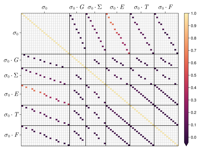
Figure 1: Example for a correlation matrix. The correlations between the data points of the unpolarized differential cross-section $\sigma_{0}$ and the used profile functions, as well as the correlation between the profile functions themselves, is shown for $E^{\text{lab}}_{\gamma}=750$ MeV. Each square represents a certain data point. The color encodes the correlation strength ranging from $-1$ (darker colors) to $+1$ (lighter colors).

The correlations are quite small, with absolute values below $\sim 0.17$, but typically in the order of $10^{-2}-10^{-3}$. An exception is the significantly higher correlation between $\sigma_{0}$ and $\sigma_{0}\cdot E$, with minimal and maximal values of $\sim 0.29$ and $\sim 0.67$, respectively. This can be explained by the similar definition of the coefficients $\mathcal{A}^{\alpha}_{k}(W)$ of $\sigma_{0}$ and $\sigma_{0}\cdot E$. Both having sensitivity to almost the exact same interference terms of multipoles, albeit with different strengths (see Ref. [19]). The magnitude of the correlation matrix elements as a function of the energy can be seen in Fig. 2.

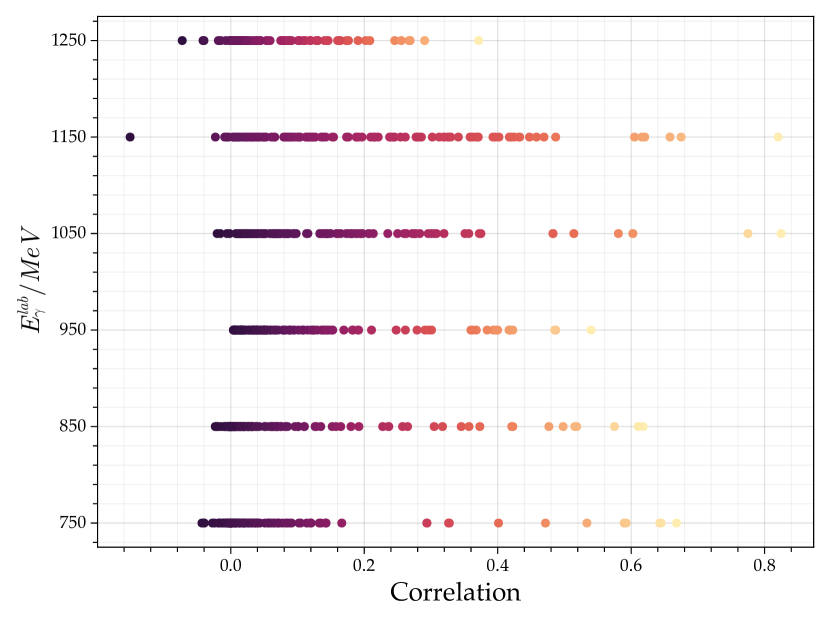
Figure 2: Unique correlation matrix element values as a function of the lab frame energy. The color encodes the correlation strength ranging from $-1$ (darker colors) to $+1$ (lighter colors).

The corresponding covariance matrix, which is used to construct the likelihood distribution in Section VI.1, can be estimated via Eqs. 46 and 47 in Appendix C.

V Underlying assumptions

An enormous strength of Bayesian statistics is its clarity about the underlying assumptions and how these evolve into the used statistical model. In general one has $N$ data-pairs $\quantity(y,x)_{i}$, where the two components can be distinguished as follows:

1. The random variables ${\bf\it y}=\quantity(y_{1},\dots,y_{N})$ follow a certain distribution. In this context, these correspond to the values of the profile functions of the polarization observables $\check{\Omega}^{\alpha}(W,\theta)$.

2. The explanatory variables [28] ${\bf\it x}=\quantity(x_{1},\dots,x_{N})$ do not belong to any probability distribution. In this context, these are the angular values $\cos(\theta_{i})$ at which the $y_{i}$ were measured.

The underlying distribution of ${\bf\it y}$ is of upmost importance as it defines the shape of the likelihood function and, by association, the structure of the parameter space. It is therefore essential to examine the distribution from which ${\bf\it y}$ originates and discuss the validity of the involved assumptions. Hereby, an understanding of the data-taking as well as the subsequent analysis, to extract values for the polarization observables, is mandatory. For this reason, special emphasis is placed on their discussion within this paper.

The polarization observables used within this analysis, originate from measurements at multiple experimental facilities: ELSA [5], MAMI [49] and GRAAL [50]. The measured quantities are count rates, corresponding to differential cross-sections, from which then, one or multiple polarization observables can be extracted. The two most common methods are a ’binned chi-square fit’ and an ’unbinned maximum-likelihood fit’ [45]. For the first case, it is common to use an asymmetry of the form:

$$A\propto\frac{N_{1}-N_{2}}{N_{1}+N_{2}},$$ (13)

where $N_{1},N_{2}$ are normalized count rates of reconstructed $\gamma p\rightarrow\eta p$ events for different polarization states [44, 43]. This has the advantage that systematic effects for example from the reconstruction efficiency cancel out.

Certainly, the distribution of this asymmetry is not explicitly addressed in any of the analyses, concerning polarization observables, which the authors have encountered up to this point. However, since the distribution of $A$ determines the structure of the likelihood distribution, it is mandatory to study its proper form.

The count rates $N_{1},N_{2}$ are Poisson-distributed random variables. If the expectation value, typically denoted as $\lambda$, is high enough, the distribution goes over to a Gaussian distribution. In the case of the here used data, this should be a good assumption.

The sum or difference of two independent Gaussian distributed random variables, as present in Eq. 13 is again Gaussian distributed, which can be shown for example using characteristic functions.

However, the ratio of two, eventually correlated, Gaussian distributions $Z=X/Y$ is far more complicated. A general treatment can be found in Ref. [51]. Additionally a closed form expression is given in Eq. 52, Section D.1. Indeed, there exist Gaussian shapes for the asymmetry $A$ in certain limits, but there exists also the possibility for a bimodal distribution [51]. Therefore, the shape of the asymmetry $A$ has to be checked for the absence of a bimodal structure. In order to use $\chi^{2}$ as likelihood function, the distribution should be well approximated by a Gaussian distribution. These checks can be performed by inserting the corresponding values for the expectation values ($\mu_{x},\mu_{y}$), standard deviations ($\sigma_{x},\sigma_{y}$) and correlation ($\rho$) into the formula for $Z$ and its transformation, see Ref. [51], or by using Eq. 52.

An alternative approach, where the utilization of such an asymmetry can be circumvented, is the already mentioned ’unbinned maximum-likelihood fit’. Albeit, in contrast to the first method, the detector acceptance has to be taken into account [45], which is possible [52]. Within this approach, the likelihood distribution can be modeled appropriately using Poisson distributions.

Summarizing, it is advantageous to use the ’unbinned maximum-likelihood fit’ for future analyses, in order to extract values for the polarization observables.

However, the distribution of the extracted polarization observables not only depends on the shape of the used likelihood function, but also implicitly on the method used to estimate the parameter uncertainties. Again, the distribution of the parameters is rarely explicitly discussed within papers such as the references cited in Table 2. The error analysis of MINUIT uses by default the HESSE approach [53], which assumes an asymptotic approximation to a Gaussian distribution for the parameters under consideration. Thus, it is likely that the parameters were assumed to be Gaussian distributed. Another indication in the same direction is that all data used within the present analysis (cf. Table 2) do have symmetric statistical uncertainties [42, 46, 45, 44, 43].

The profile functions $\check{\Omega}^{\alpha}$ are calculated by a product of random variables. However, even when these two random variables are independent and Gaussian distributed, the result is not always a Gaussian, only when one of the standard deviations is very small, see [18] or Section D.2. Fortunately, this is the case for $\sigma_{0}$ as it is the observable in $p\eta$-photoproduction with an unprecedented accuracy.

VI The posterior distribution

Using the knowledge of Section V, it seems reasonable to assume that the used dimensionless polarization observables, as well as the unpolarized differential cross-section, are Gaussian distributed and independent of each other. Furthermore, it seems reasonable that the profile functions are Gaussian distributed. The profile functions are correlated with the unpolarized differential cross-section, as well as among themselves, see Section IV. This dependence is modeled within the likelihood distribution using a covariance matrix. In favor of a compact representation, the functional dependencies are not shown explicitly in the subsequent equations.

VI.1 Likelihood distribution

Combining the results of Sections IV and V, the conditional likelihood distribution, for each of the analyzed energies, can be formulated as an $N$-dimensional multivariate Gaussian distribution:

$$p({\bf\it y},{\bf\it x}\mid{\bf\it\Theta},{\bf\it\kappa}) =\mathcal{N}({\bf\it\mu}({\bf\it\Theta},{\bf\it\kappa},{\bf\it x}),{\bf\it\Lambda})$$

$$=\frac{\exp(-\frac{1}{2}\quantity({\bf\it y}-{\bf\it\mu})^{\mathrm{T}}{\bf\it\Lambda}^{-1}\quantity({\bf\it y}-{\bf\it\mu}))}{\sqrt{(2\pi)^{N}|{\bf\it\Lambda}|}}.$$ (14)

Hereby, the vectors ${\bf\it x},{\bf\it y}\in\mathbb{R}^{N}$ contain the entirety of the $N\in\mathbb{N}$ used polarization observable data points and the corresponding angular values at which they were measured, respectively:

$${\bf\it y} =[{\bf\it y}^{\sigma_{0}},{\bf\it y}^{\check{G}},{\bf\it y}^{\check{\Sigma}},{\bf\it y}^{\check{E}},{\bf\it y}^{\check{T}},{\bf\it y}^{\check{F}}],$$ (15)

$${\bf\it x} =[{\bf\it x}^{\sigma_{0}},{\bf\it x}^{\check{G}},{\bf\it x}^{\check{\Sigma}},{\bf\it x}^{\check{E}},{\bf\it x}^{\check{T}},{\bf\it x}^{\check{F}}].$$ (16)

The parameters of the model can be divided into two groups. On the one hand, the real- and imaginary parts of multipoles, i.e. Eq. 4, denoted by ${\bf\it\Theta}\in\mathbb{R}^{8\ell_{\text{max}}-1}$ are used to model the underlying physical process. On the other hand, the parameters ${\bf\it\kappa}\in\mathbb{R}^{5}$ which are used to model the systematic uncertainties of the involved data sets:

$${\bf\it\kappa}=[\kappa^{\sigma_{0}},\kappa^{\check{G}},\kappa^{\check{E}},\kappa^{\check{T}},\kappa^{\check{F}}].$$ (17)

The multivariate normal distribution in Eq. 14 is constructed with the model predictions ${\bf\it\mu}\in\mathbb{R}^{N}$ for the expectations of ${\bf\it y}$:

$${\bf\it\mu}({\bf\it\Theta},{\bf\it\kappa},{\bf\it x})=[ \kappa^{\sigma_{0}}\cdot{\bf\it\mu}^{\sigma_{0}},\kappa^{\check{G}}\cdot{\bf\it\mu}^{\check{G}},1\cdot{\bf\it\mu}^{\check{\Sigma}},$$

$$\kappa^{\check{E}}\cdot{\bf\it\mu}^{\check{E}},\kappa^{\check{T}}\cdot{\bf\it\mu}^{\check{T}},\kappa^{\check{F}}\cdot{\bf\it\mu}^{\check{F}}].$$ (18)

The ${\bf\it\mu}^{\alpha}({\bf\it\Theta},{\bf\it x}^{\alpha})$ are the model predictions for the individual profile functions, i.e. Eq. 2. Hence, in order to model the systematic uncertainties, one additional parameter per relevant data set is introduced and multiplied with the corresponding theoretical prediction for the profile function. Thus, the model gets additional degrees of freedom to adjust for possible systematic uncertainties. However, these parameters are restricted to physical meaningful bounds, further discussed in Section VI.2. As explained in Section IV, the systematic uncertainty of the polarization observable $\Sigma$ can not be modeled.

Finally, there is the covariance matrix ${\bf\it\Lambda}\in\mathbb{R}^{N\times N}$. Its off-diagonal terms are not identical, and therefore the data-pairs are not exchangeable. This will become relevant when discussing the predictive performance in Section VII.5.

VI.2 Prior distribution

The priors for the multipole parameters are chosen as uniform priors with bounds corresponding to the physically allowed ranges of the parameters (see [18]). Thus, the priors incorporate physical knowledge while being uninformative compared to the likelihood distribution.

In principle a uniform prior for the systematic parameters would be reasonable. However, in this case the hard boundaries in the parameter space lead to numerical issues. Thus, the prior distributions for the scaling parameters ${\bf\it\kappa}$ are assumed to be normal distributed, and centered around the value one. The standard deviation is chosen such that $99\%$ of the distribution are within the range $1\pm\Delta^{\alpha}_{\text{sys}}$, which results in (rounded to five digits):

$$\kappa^{\sigma_{0}} \sim\mathcal{N}(1,0.01552),$$ (19)

$$\kappa^{\check{G}} \sim\mathcal{N}(1,0.04542),$$ (20)

$$\kappa^{\check{E}} \sim\mathcal{N}(1,0.03882),$$ (21)

$$\kappa^{\check{T}} \sim\mathcal{N}(1,0.03222),$$ (22)

$$\kappa^{\check{F}} \sim\mathcal{N}(1,0.04076).$$ (23)

This choice is in accordance with the conservative combination of the systematic uncertainties as discussed in Section IV. The treatment of systematic errors within this paper is similar to that in Refs. [55, 56, 38].

VII Analysis steps

This section explains in detail the analysis steps in order to determine the complex multipole parameters using Bayesian statistics, from which predictions of polarization observables are then obtained.

The posterior, which may in many cases be explicitly multimodal, and the goal to analyze the structure of the mathematical ambiguities, bear a major challenge with respect to the sampling of the posterior distribution.

On the one hand, posteriors with multiple modes connected by regions of low posterior density persuade the Markov chains to get stuck within a certain mode, unable to explore multiple ones [28]. This results in drastically failing Markov chain Monte Carlo convergence diagnostics, such as the potential-scale-reduction statistic $\hat{R}$.

On the other hand, the number of possible modes increases exponentially with the truncation order $\ell_{\text{max}}$. An upper limit can be given by $2^{4\ell_{\text{max}}}-2$, as this is the maximal possible number of accidental ambiguities of the four group $\mathcal{S}$ observables (note that the bulk of this number is probably not realized as actual ambiguities, due to the multiplicative constraint Eq. 10) [18]. Capturing consistently all modes of the marginal posterior distributions via a large number of chains, with randomized starting values is computationally inefficient. Furthermore, randomized starting values will lead to traceplots where one can not distinguish between chains that have not converged yet and chains which have explored more than one mode. An illustrative example is shown in Fig. 3.

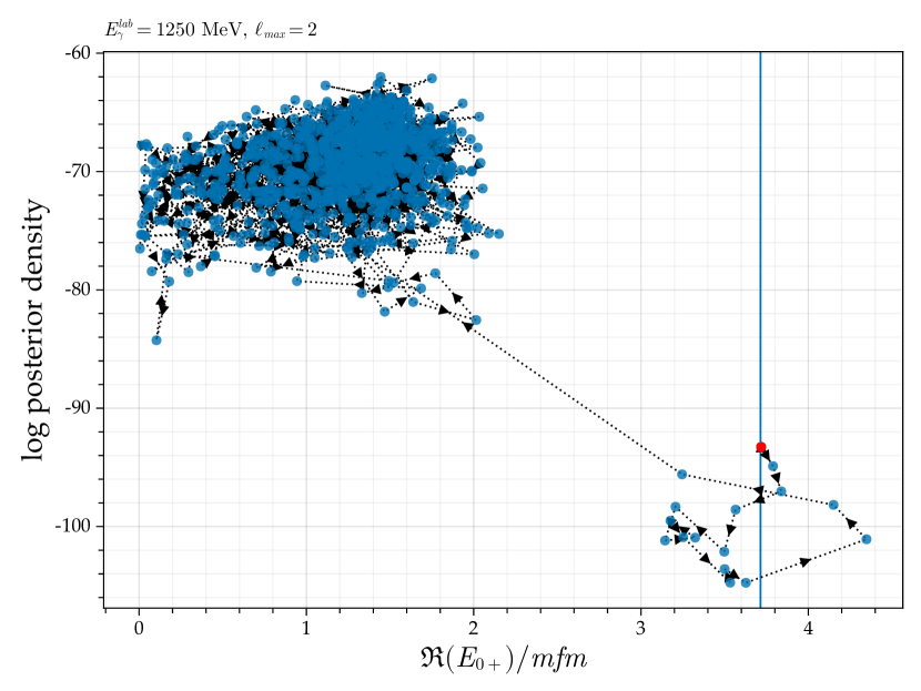
Figure 3: Illustration of the first 1000 sampling points of a chain with initial value at $3.7$ (the blue vertical line). The first sampling point is drawn in red. The chain converges from its starting point to a more likely solution, i.e. with higher log posterior density value.

These difficulties can be overcome by specifying well chosen starting values for the Markov chain Monte Carlo algorithm, explained in more detail in Sections VII.2 and VII.3. On that account, certain parts of the typical Bayesian workflow [57] have to be adapted.

VII.1 Monte Carlo maximum a posteriori estimation

In order to compare between different solutions, found within the same analysis, it is important to find all modes of the marginal posterior distributions, especially the global maximum.

As already mentioned, the number of accidental ambiguities rises exponentially with the truncation order. Thus, the utilization of an optimization routine is substantially more efficient than a large number of Markov chain Monte Carlo chains. With this in mind, a Monte Carlo maximum a posteriori estimation of the proposed posterior is employed as a preparatory step for the Bayesian inference procedure. The results of the following approach are cross checked via an implementation in Mathematica [58], using the Levenberg-Marquard-algorithm [59, 60], as well as in Julia [61], using the L-BFGS-algorithm [62, 63, 64, 65, 66] via Optim.jl [67].

At first, one needs to fix the overall phase of the multipoles, due to the bilinear product in Eq. 3. Indeed, without such a constraint the minimization algorithms would have convergence problems, as the solutions are no longer located at isolated points in the parameter space but on continuous connected regions. Without loss of generality, a valid choice is $\real(E_{0+})>0$, $\imaginary(E_{0+})=0$ [18].

Second, the minimization algorithm is performed for $n$ different starting values. The starting values are chosen within the physically allowed parameter space, which solely depends on the total cross-section $\sigma_{\text{tot}}$ [18, 68]. Fortunately, the unpolarized differential cross-section is the most accurately measured observable in $p\eta$-photoproduction [1], thus yielding accurate limits. An appropriate amount of $n$ equidistant points is chosen on each axis of this $8\ell_{\text{max}}-1$ dimensional hyper-rectangle, such that the volume is sufficiently covered. Each of these parameter configurations is then used as starting values for the minimization algorithm.

Finally, the non redundant solutions, of the $n$ possible mode candidates, can be extracted via a clustering algorithm. Hereby, all values of the multipole parameters are rounded to six digits. Then the unique solution vectors can be filtered out.

A rough estimate for the uncertainty of each parameter solution is calculated via the inverse of the Hesse matrix [69], i.e. assuming a Gaussian shape of the parameters.

VII.2 Sampling of the posterior

Within this work, the well established probabilistic programming software Stan [70] has been used to encode the employed model and to run the posterior sampling with the state-of-the-art Hamiltonian Monte Carlo algorithm [31, 32] in combination with the No-U-Turn sampler [71]. The employed Stan model can be found in the supplementary material Ref. [72].

For each mode of the posterior distribution, determined within Section VII.1, $N_{\text{c}}$ chains are sampled with starting values for the multipole and systematic parameters equal to the corresponding $(8\ell_{\text{max}}+4)$-dimensional solution vector. This approach ensures adequate sampling of all marginal posterior modes and enables again a meaningful convergence diagnostics, further discussed in Section VII.3. Hence, this is true as long as the posterior modes are in the vicinity of the ’typical set’ , which is the case within this paper.

The following tuning-parameters of the Hamiltonian Monte Carlo algorithm and the No-U-Turn sampler are adapted to the problem at hand. The average Metropolis acceptance probability $\delta\in[0,1]$ is increased from its default value of 0.8 to $\delta=0.99$. Thus, preferring a more fine-grained sampling, i.e. smaller leapfrog steps $\epsilon$ [71], over the additional computation time. The maximum tree depth, with a default value of 10, is increased to 50, so that the algorithm can explore even challenging posterior regions without hitting the termination conditions [70].

VII.3 Monitor Markov chain Monte Carlo convergence

Naturally one is interested in how well the structure of the posterior was explored by the applied Markov chain Monte Carlo algorithm. The goal is to diagnose whether all Markov chains have explored the same part of the posterior distribution [28], i.e. whether the obtained distribution is reliable or accrued due to a random effect. This can be monitored by convergence diagnostics such as the potential-scale-reduction statistic $\hat{R}$ [34] and Monte Carlo standard error [33] (which depends on the effective sample size [28]). Within this work, the adapted versions of these diagnostics, as proposed by Vehtari et al. [74], are employed. In addition, trace plots [35] can be used to monitor the behavior of chains which explore multiple marginal modes. For each of these diagnostics, it is essential to use multiple chains [74, 35] for a reliable result.

However, a multimodal posterior provides some pitfalls. As already mentioned at the beginning of Section VII, the Markov chains can get stuck in certain, isolated modes. Thus not all chains would have seen the same parts of the posterior distribution and the convergence diagnostics would indicate that the chains have not converged.

Therefore, in case a multimodal posterior is studied, where all modes are of interest, the usual methods are not applicable. An adaptation has to be made. Under the assumption that all modes of the posterior were found via Monte Carlo maximum a posteriori estimation, see Section VII.1, the following strategy is employed. A schematic representation of the adapted approach can be found in Fig. 4.

Figure 4: Adapted workflow to monitor Markov chain Monte Carlo convergence due to a multimodal posterior.

Instead of applying the convergence diagnostics to all chains at once, the chains are clustered into groups according to their sampled parameter space and the convergence diagnostics are then applied onto each group separately. Consequently, the convergence for the whole posterior is monitored.

The chains can be grouped according to their similarity as follows: To avoid problems during the clustering process, coming from high dimensional data [76], a dimensional reduction of the chains is performed. Each chain, consisting of $S$ sampling points, is characterized via a vector of its quantiles, in this case the $[0.1,0.2,0.3,0.4,0.5,0.6,0.7,0.8,0.9]$ - quantiles. Subsequent, the corresponding distance matrix [77] of the quantile vectors is calculated using the Euclidean metric. The constructed matrix serves as input for the DBSCAN algorithm [78]. The minimal cluster size should be at least two, as this is the minimal amount of chains required to perform the $\hat{R}$ diagnostic [35]. An appropriate $\epsilon$ - neighborhood for the DBSCAN algorithm can be graphically determined, for example by visualizing the Euclidean distances of the quantile vectors to each other. Afterwards, the correct clustering of chains can be checked visually. Alternatively, the two-sample Kolmogorov-Smirnov test [79, 80] or the K-Sample Anderson–Darling test [81] could be employed to compare two distributions with each other.

The outlined approach still allows to adjust the number of chains $N_{\text{c}}$ per group and the sampling points $S$ in order to gain adequate convergence diagnostics and the desired precision for the parameter estimates. Within this paper, one is aiming for $\hat{R}<1.01$ [74] and a relative Monte Carlo standard error in the region of a few percent.

VII.4 Posterior predictive check

In general, a posterior predictive check [28] is useful for determining flaws within the Bayesian analysis, such as problematic data points, programming errors, systematic effects or the inadequacy of the employed model. Furthermore, it allows for a more detailed investigation of the ambiguities, as it helps to clarify if a clear distinction between the different solutions is even possible. In conjunction with this, it is possible to check whether additional measured observables could resolve the ambiguity. Furthermore, predictions of polarization observables, which were not included within the analysis, can be calculated.

The central component is the probability distribution of reproduced data points ${\bf\it y}^{\text{rep}}$ given the used data ${\bf\it y}$, which is called the posterior predictive distribution [28, 37]:

$$p({\bf\it y}^{\text{rep}}\mid{\bf\it y}) =\mathbb{E}_{{\bf\it\Theta}}\quantity[p\quantity({\bf\it y}^{\text{rep}}\mid{\bf\it\Theta})],$$

$$=\int p({\bf\it y}^{\text{rep}}\mid{\bf\it\Theta})p({\bf\it\Theta}\mid{\bf\it y})\differential{{\bf\it\Theta}},$$ (24)

where $\mathbb{E}_{{\bf\it\Theta}}[\ldots]$ denotes the expectation value over the parameter-vector ${\bf\it\Theta}$. Hence, this allows to compare each data point $y_{i}$ directly with its corresponding replicated marginal distribution $p(y^{\text{rep}}_{i}\mid{\bf\it y})$. Both should look similar under a reasonable model [28]. Irregularities, such as outliers or statistically weak data points, can be detected.

As in the last section, the posterior predictive check is performed for each group of chains. Hence, one can check if different marginal modes give the same posterior predictive distribution, which is indeed very helpful to determine potentially harmful ambiguities.

VII.5 Predictive performance

In principle, predictive performance could be used to compare different solutions found within the same analysis or even different models. However, as described in Section IV, the statistical analysis takes correlations between the used data points into account. As a consequence, the off-diagonal elements of the calculated covariance matrices, for all six energies, are non-identical. Thus, the data pairs $(y,x)_{i}$ are no longer exchangeable. Unfortunately, methods like cross-validation [28] or information criteria like the widely applicable information criterion [37] are not applicable any more in order to estimate the predictive performance. This is explained in detail in Appendix E.

As an alternative approach to compare different solutions, found within one specific analysis, the log posterior density distributions are used. It is assumed that higher log posterior density values correspond to more likely parameter values (within one specific analysis).

VII.6 Analysis of generated data

It is crucial to prove the correct implementation and validity of the used model. An ideal testing scenario would be the a priori knowledge of the correct outcome of the analysis using the model under consideration. Therefore the partial-wave analysis solution EtaMAID2018 [82] is employed for the electromagnetic multipoles in Eq. 4 up to the desired truncation order $\ell_{\text{max}}$. By these means, pseudo data for the profile functions $\check{\Omega}^{\alpha}(W,\theta)$ can be generated via Eq. 2 for certain energies and angular positions for the observables $\sigma_{0}$, $\Sigma$, $T$, $E$, $F$ and $G$. These data are then used as input for the truncated partial-wave analysis following the described steps in Sections VII.1, VII.2, VII.3 and VII.4. The analysis should yield again the EtaMAID2018 multipole solutions.

VIII Results

In a first step, Bayesian inference was applied to the generated data, see Section VII.6, and was successful in extracting the EtaMAID2018 multipole solutions again. In a second step, Bayesian inference, i.e. the outlined approach in Sections VII.1, VII.2, VII.3, VII.4 and VII.5, was applied to the experimental data sets introduced in Section IV. The results of these analyses are discussed in the following.

The maximum a posteriori approach implemented in Julia and Mathematica gave the same results for the analyzed truncation orders and energy-bins, i.e. with two different minimization algorithms. Predictions for $H$, $P$, as well as the polarization observables of group $\mathcal{BR}$ and $\mathcal{TR}$ are generated . All predicted data distributions are within the physical bounds between -1 and 1 and their overall course over the angular range shows the correct tendency at $\cos(\theta)=\pm 1$ towards the mathematically expected values [17], see for example Fig. 15 and Ref. [72]. In general, the posterior predictive checks are plotted together with the theory values of EtaMAID2018 [82], BnGa-2019 [46] and JüBo-2022 [56].

Bayesian inference gives more insight into the relevance of ambiguities, due to the Hamiltonian Monte Carlo algorithm. When multiple chains sample consistently multiple marginal modes together, this is a sign of a problematic ambiguity, as they tend to have comparable log posterior densities. An example is shown in the top left of Fig. 12.

The presentation of the multipole parameter results is quite detailed and deserves an explanation. The top part shows the solutions found via Monte Carlo maximum a posteriori estimation and their corresponding $\chi^{2}/ndf$ values, together with the $1\sigma$-uncertainty (see Section VII.1). The middle part shows the marginal-parameter distributions obtained via Bayesian inference, as explained in Sections VI and VII.2. For a better comparison of the two approaches for $\ell_{\text{max}}=1$, the $[0.16,0.5,0.84]$-quantiles of the distributions, corresponding to the median of the distribution and the $1\sigma$-uncertainty boundaries, are drawn as dashed lines through all parts of the figure. Whereas, for $\ell_{\text{max}}=2$ a solid vertical line is drawn for each peak of the multimodal distribution, i.e. the most probable values. The bottom part of the figure is a contour plot of the log posterior density distribution and the corresponding marginal-parameter distribution. The outermost contour line is at $1\%$ of the maximum altitude, each subsequent line represents an $11\%$ increase. It is assumed that a log posterior distribution centered around a higher log posterior value, corresponds to more likely parameter values, as this solution contributes more probability mass to the posterior.

Each solution group is drawn in a different color. These colors are consistent between the shown figures (Monte Carlo convergence- , multipole-, predictive performance plots, etc.) for a certain energy and truncation order.

Within the following discussion of the results a representative selection of figures is shown. All parameter figures, for all analyzed energies and truncation orders can be found in the supplementary material Ref. [72].

VIII.1 Truncation order $\ell_{\text{max}}=1$

The number of warmup and post-warmup samples are set to $2\crossproduct 10^{4}$, respectively, for each of the six energy-bins. The number of chains started at each solution, found via the Monte Carlo maximum a posteriori approach, is set to $N_{\text{c}}=10$. The corresponding convergence diagnostics, which are shown in Appendix F, Fig. 17, validate this choice, i.e. $\hat{R}<1.01$ and a relative Monte Carlo standard error in the region of a few percent or less. The following discussion is separated according to two sets of energy-bins, in each of which the analyses exhibit a certain behavior.

VIII.1.1 $E^{\text{lab}}_{\gamma}=[750,850,950]$ MeV

For the energies in the neighborhood of the $\eta p$ production threshold one has two distinct groups of chains. The corresponding log posterior density distributions are clearly distinguishable. A typical example is shown at the top of Fig. 5. The estimated parameter values associated with the curves around $-50$ are more likely than the ones corresponding to the curves around $-90$.

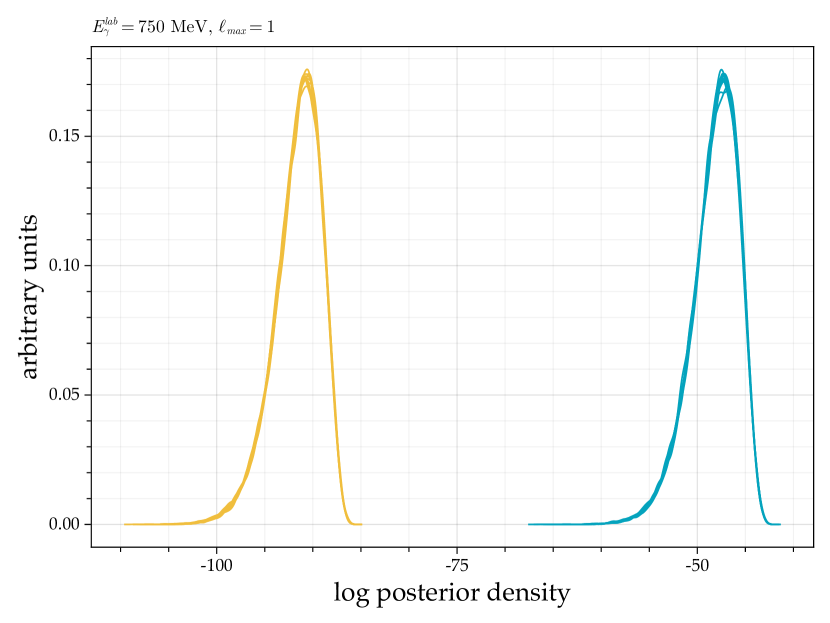
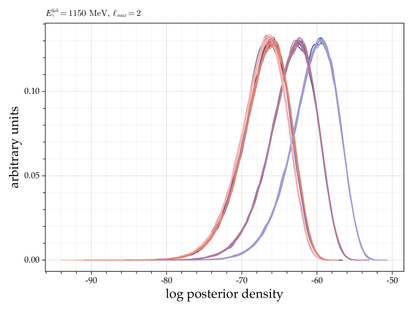
Figure 5: Examples for log posterior density distributions. Top) Two groups of chains with clearly distinct distributions, $E^{\text{lab}}_{\gamma}=750$ MeV and truncation order of $\ell_{\text{max}}=1$. Bottom) Five groups of chains with similar distributions, $E^{\text{lab}}_{\gamma}=1150$ MeV and truncation order of $\ell_{\text{max}}=2$.

The interpretation is that all $N_{\text{c}}$ chains of one starting value configuration explore exclusively the same single mode. Hence, the two modes are disconnected by regions of low probability, thus the chains are unlikely to explore both modes [32].

In general, the sampled marginal-parameter distributions from Bayesian inference share the median and $1\sigma$-uncertainty very well with the solutions of the Monte Carlo maximum a posteriori approach. The multipole parameters $\real(E_{0+})$ and $\imaginary(M_{1-})$ are shown as examples in Fig. 6 in place of the other multipole parameters, which show a similar behavior (see Ref. [72]).

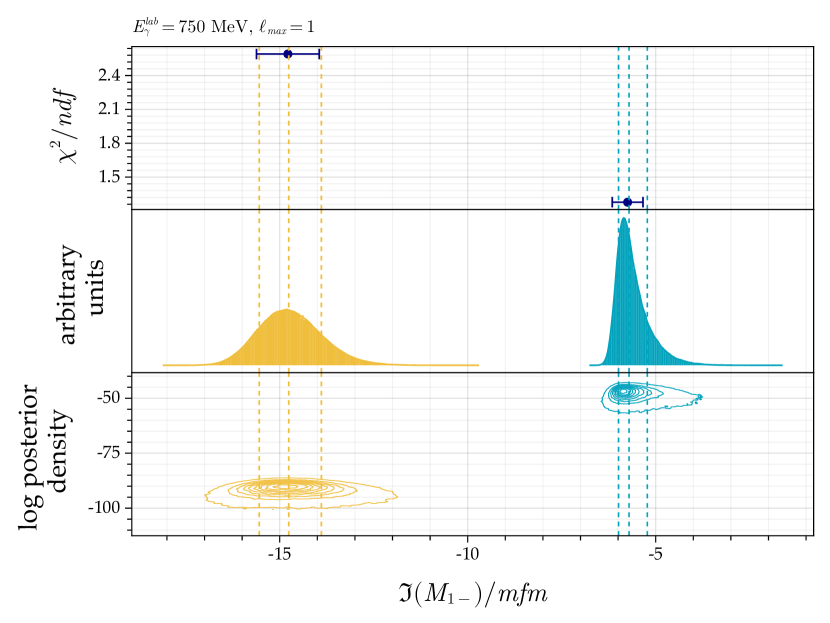
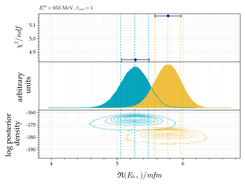
Figure 6: Parameter distributions for the multipoles $\imaginary(M_{1-})$ at $E^{\text{lab}}_{\gamma}=750$ MeV and $\real(E_{0+})$ at $E^{\text{lab}}_{\gamma}=950$ MeV for a truncation order of $\ell_{\text{max}}=1$. The corresponding log posterior density and the solutions found via the Monte Carlo maximum a posteriori approach, as explained in Section VII.1, are shown as well. Further illustrations can be found in the supplementary material Ref. [72].

The reproduced data distributions can be seen in Fig. 7 and show an interesting behavior.

Figure 7: Posterior predictive check for the profile functions $\sigma_{0},\check{G},\check{\Sigma},\check{E},\check{T}$ and $\check{F}$, for truncation order $\ell_{\text{max}}=1$ and energy-bins $E^{\text{lab}}_{\gamma}=\quantity[750,850,950,1050,1150,1250]$ MeV. The reproduced data distributions for the different solutions are shown together with the original data with statistical uncertainties as black points. In addition, the corresponding values from EtaMAID2018 [82] (dashed line), BnGa-2019 [46] (dotted line) and JüBo-2022 [56] (dash-dotted line) are shown as well.

For the unpolarized differential cross-section $\sigma_{0}$ and the profile functions $\check{G},\check{\Sigma}$ and $\check{E}$ the posterior predictive check looks reasonable, as it resembles the original data and do not show significant evidence of overfitting nor systematic effects. However, the different distributions are hardly distinguishable. In contrast, the distributions for the different solutions for $\check{T}$ and $\check{F}$ can be clearly distinguished. It seems that certain outliers in the original polarization observable data facilitate the emergence of an ambiguity, because these outliers are not able to exclude either of the two mathematical descriptions. Thus, a remeasurement or a reanalysis of $\check{T}$ or $\check{F}$ could be able to resolve the remaining mathematical ambiguity.

VIII.1.2 $E^{\text{lab}}_{\gamma}=[1050,1150,1250]$ MeV

These energies do not show any mathematical ambiguities, i.e. there is exactly one group of chains. The maximum a posteriori approach and Bayesian inference yield again very similar results, see Ref. [72].

The posterior predictive checks for the profile functions look reasonable (no overfitting, no systematic effects visible), with the two exceptions $\sigma_{0}$ and $\check{\Sigma}$. At each of the three energy bins, the measured data for $\sigma_{0}$ are systematically higher for $\cos(\theta)>0$ than the model predictions would suggest and for $\check{\Sigma}$ it seems they do not resemble the original data points at all, see Fig. 7. It seems that the employed statistical model with truncation order $\ell_{\text{max}}=1$ is not able to reproduce data points for all observables equally well. This behavior could be explained by an emerging resonance in the energy range between $950$ and $1050$ MeV, which couples to a higher orbital angular momentum and contributes predominantly to $\sigma_{0}$ and $\check{\Sigma}$.

The reaction of $\eta$-photoproduction acts as an isospin-filter due to the isospin conservation in the strong interaction, therefore only $N^{*}$ resonances are relevant for the following discussion. There are two $N^{*}$ resonances which fulfill the conservation laws, couple to $\ell_{\text{max}}=2$ and are within the required energy range (taking into account the Breit-Wigner width [2] of the resonances), namely $N(1675)5/2^{-}$ [2] at $E^{\text{lab}}_{\gamma}\approx 1026$ MeV and $N(1700)3/2^{-}$ [2] at $E^{\text{lab}}_{\gamma}\approx 1071$ MeV. There is also a resonance which opens up already at $E^{\text{lab}}_{\gamma}\approx 762$ MeV namely $N(1520)3/2^{-}$ [2]. However, this resonance has a $\sim 10$ times smaller branching ratio to $\eta N$ [2] than the two previously mentioned resonances and the used data sets do not seem to provide the required sensitivity for it.

As the applied theoretical model is not able to reproduce the used data, neither the predicted observable distributions nor multipole or systematic parameters are shown here, but can be found in the supplementary material Ref. [72].

VIII.2 Truncation order $\ell_{\text{max}}=2$

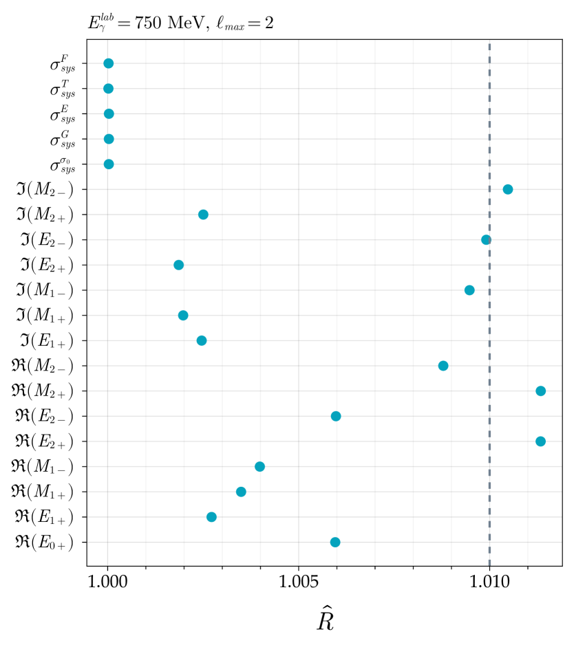
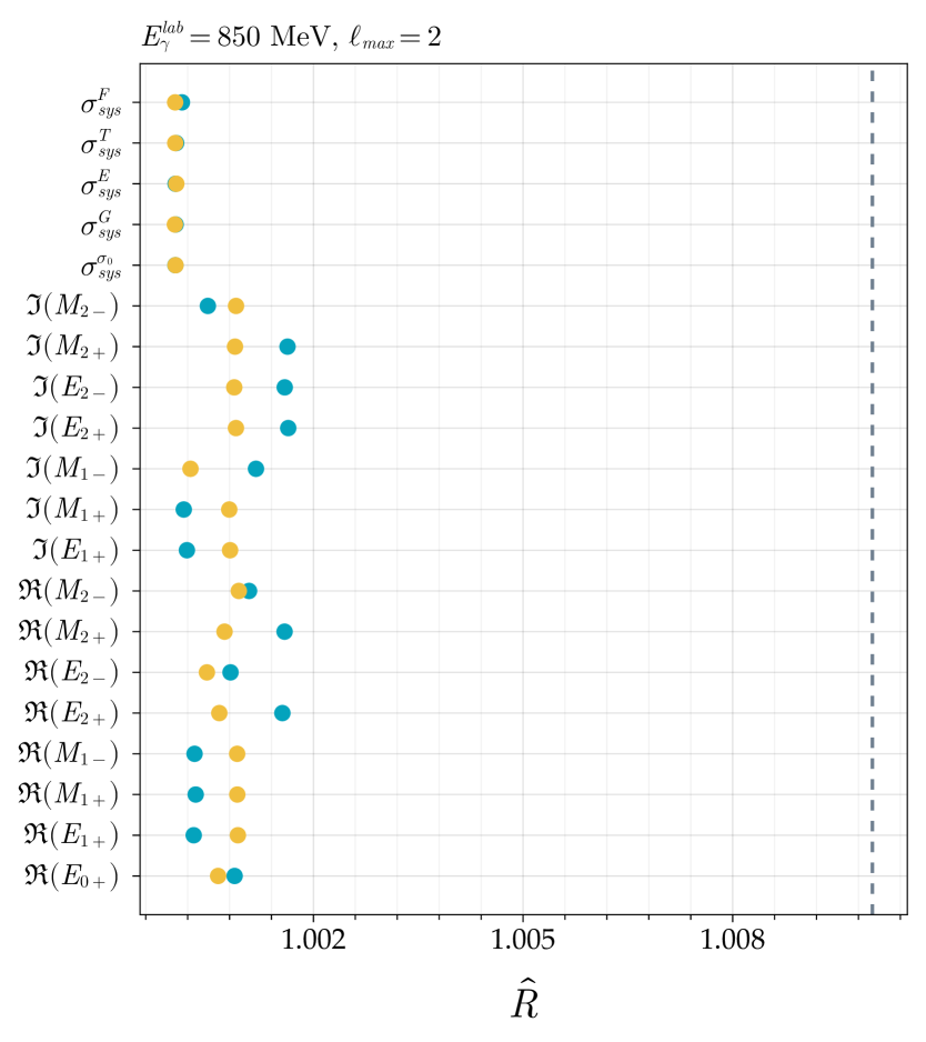
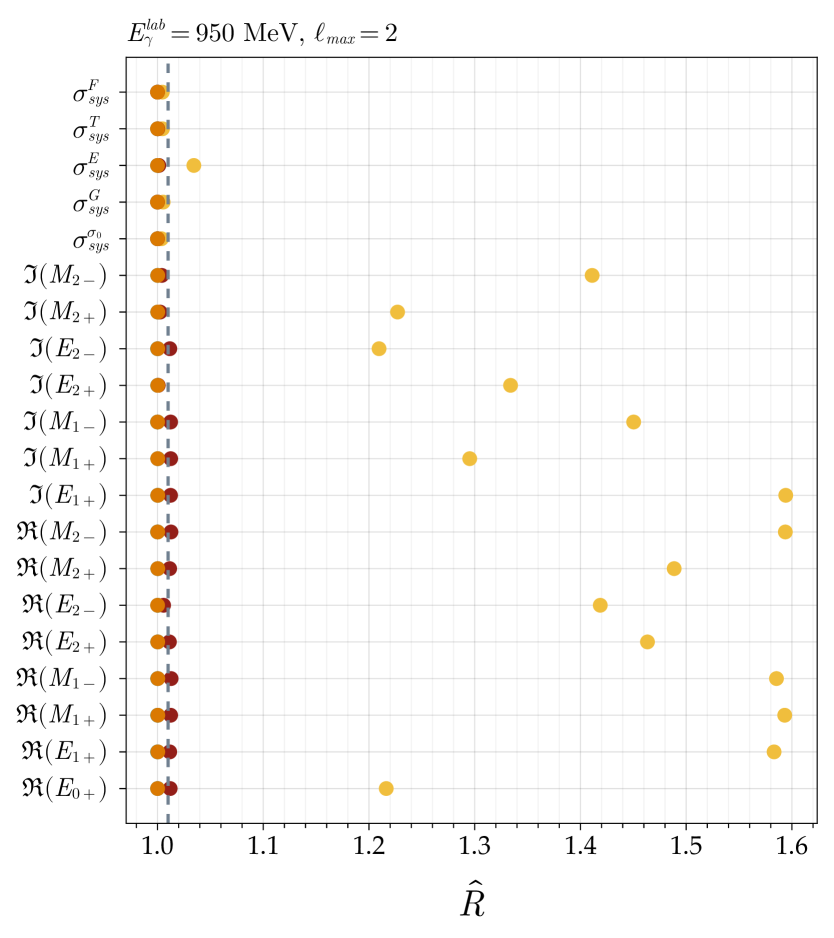
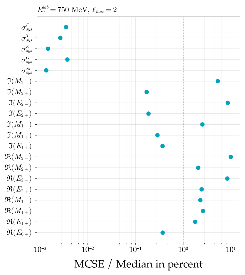
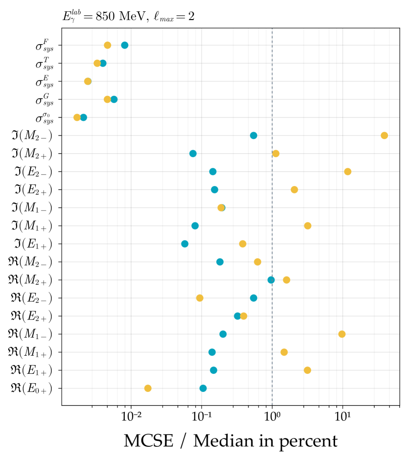
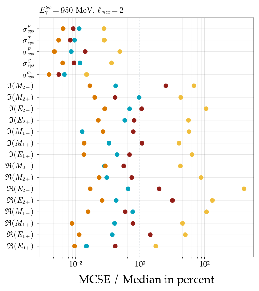
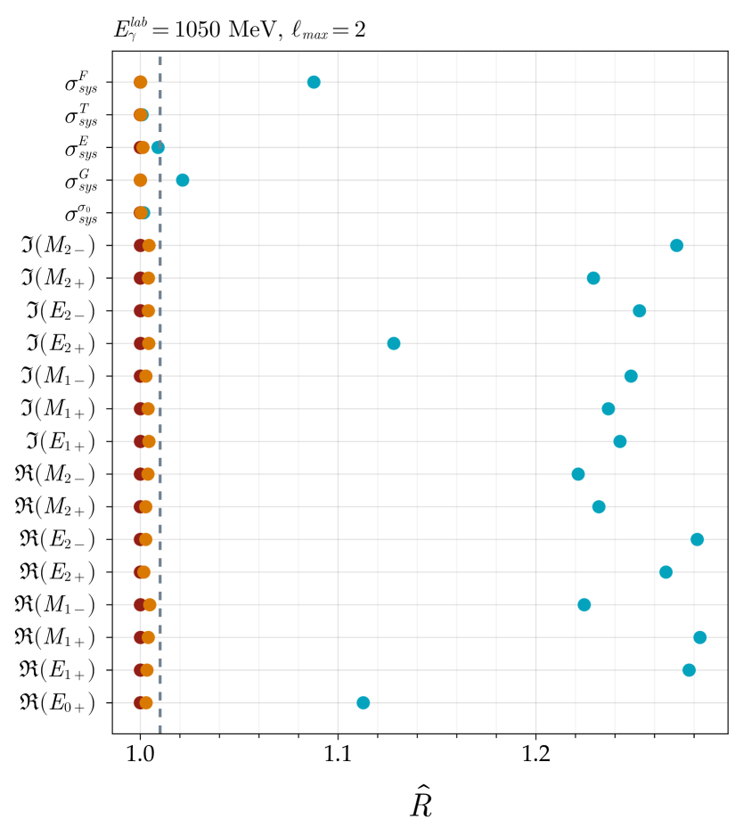
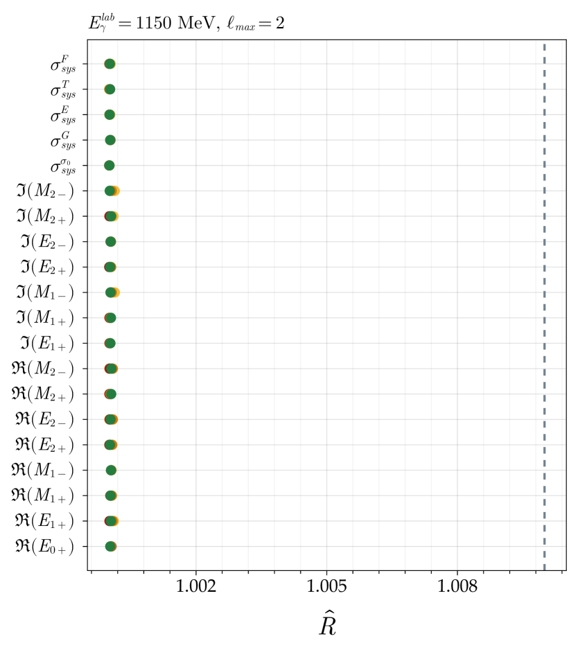
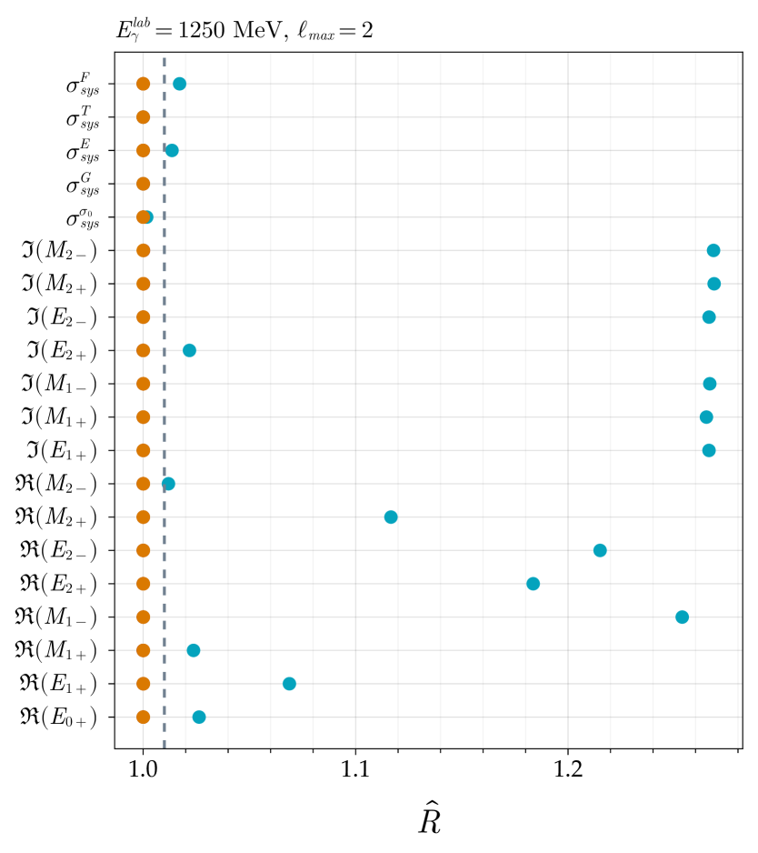
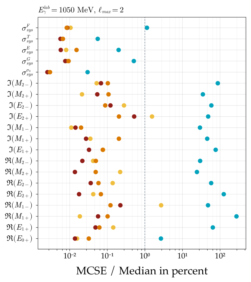
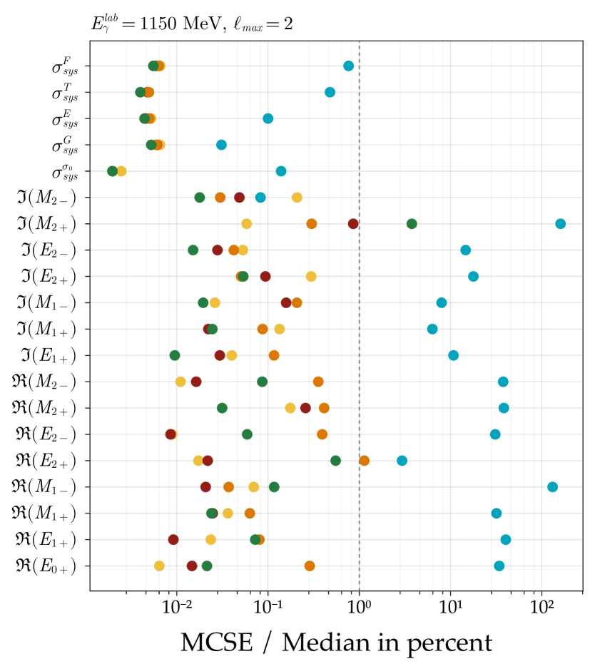
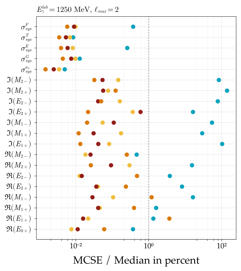
Figure 18: Markov chain Monte Carlo convergence diagnostics for the truncation order $\ell_{\text{max}}=2$. Shown are the potential-scale-reduction statistic $\hat{R}$ (the grey, dashed line indicates the value of 1.01) and the Monte Carlo standard error (MCSE) for the median divided by the median in percent (the grey, dashed line indicates the value of $1\%$).

The number of warmup and post-warmup samples are increased to $5\crossproduct 10^{4}$, respectively, for each of the six energies. The number of chains, started at each solution, found via the Monte Carlo maximum a posteriori approach, is set to $N_{\text{c}}=10$. The corresponding convergence diagnostics, which are shown in Appendix F, Fig. 18, validate this choice, i.e. $\hat{R}<1.01$ and a relative Monte Carlo standard error in the region of a few percent. The diagnostics for $750$ MeV are fine, despite their slightly increased values, caused by the highly multimodal marginal parameter distribution.

In general, the log posterior density distributions are less separated in comparison to $\ell_{max}=1$, an example is shown at the bottom of Fig. 5.

There are several phenomena appearing at this truncation order, which are discussed in the following:

1)

The convergence diagnostics, see Fig. 18, for the four energies $E^{\text{lab}}_{\gamma}=[950,1050,1150,1250]$ MeV look suspicious. In each case one group of chains show $\hat{R}$-values way above 1.01 and relative Monte Carlo standard errors of over $100\%$. This results from two modes separated in phase space by a small region of low probability, so that the Metropolis acceptance probability [32] for a transition between the two high probability regions is quite small but nonzero. Hence, just a small number of chains is able to explore both marginal modes at once, which is the reason for the suspicious convergence diagnostics. For the case of $1050$ MeV, the blue distribution corresponds to a cluster with just one group member. Hence, it is not possible to calculate an $\hat{R}$-value for this cluster. It is important to note that this behavior can not be prevented as it is inherently a random effect. As an example how this phenomenon manifests within a parameter distribution, see the blue distributions of $\imaginary(M_{1+})$ and $\imaginary(M_{2+})$ in Fig. 8.

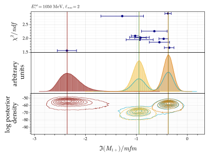
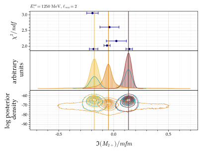
Figure 8: Examples for a group of chains with inadequate Markov chain Monte Carlo convergence diagnostics, i.e. the orange distribution (left) and the cyan distribution (right). Compare this with the corresponding diagnostics in Fig. 18. The different parts of the tripartite plots are explained at the beginning of Section VIII. Further illustrations can be found in the supplementary material Ref. [72].

Despite their convergence diagnostics, these types of distributions are shown within the multipole parameter and posterior predictive plots for their illustrative purposes.

2)

The truncated partial-wave analysis with $\ell_{\text{max}}=2$ is able to reproduce the data points for all used profile functions for all energies, as can be seen in Fig. 9. Indeed the used model is now able to describe the data points for $\sigma_{0}$ and $\check{\Sigma}$ for $E^{\text{lab}}_{\gamma}=[1050,1150,1250]$ MeV, in contrast to $\ell_{\text{max}}=1$.

Figure 9: Posterior predictive check for the profile functions $\sigma_{0},\check{G},\check{\Sigma},\check{E},\check{T}$ and $\check{F}$, for truncation order $\ell_{\text{max}}=2$ and energy-bins $E^{\text{lab}}_{\gamma}=\quantity[750,850,950,1050,1150,1250]$ MeV. The reproduced data distributions for the different solutions are shown together with the original data with statistical uncertainties as black points. In addition, the corresponding values from EtaMAID2018 [82] (dashed line), BnGa-2019 [46] (dotted line) and JüBo-2022 [56] (dash-dotted line) are shown as well.

3)

As the two former points validate the Markov chain Monte Carlo sampling and the employed model, the multipole results can be studied. As to be expected, in comparison to truncation order $\ell_{\text{max}}=1$, more ambiguities emerge. Their corresponding log posterior distributions, likewise $\chi^{2}/ndf$-values, have moved closer together in terms of their range of values. Thus, in some cases the most likely solution can not be determined. Each marginal distribution, for all systematic parameters, for all analyzed energy-bins, is exclusively unimodal. Examples are shown in Fig. 10, see also Ref. [72]. The solutions for $E_{0+}$ and $M_{2+}$ are shown as representative examples of the multipole parameters in Figs. 11, 12 and 13. The solutions for all multipole parameters can be found in Ref. [72]. Typically, the peaks of the marginal distributions are in agreement with the first few ’best’ a posteriori estimates. However, not every a posteriori solution has a corresponding peak within the marginal distributions. The reason could be twofold. On the one hand, the interpretation of a marginal distribution differs from that of a maximum a posteriori estimate. On the other hand, the reason might be in the Hamiltonian Monte Carlo algorithm [31, 32], i.e. it is observed that some of the starting values are not in the direct vicinity of the ’typical set’ [73] but adjust rather quickly. An example is shown in Fig. 3.

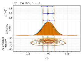
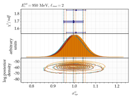
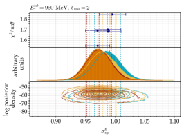
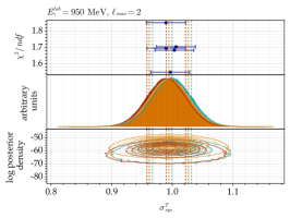
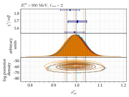
Figure 10: Examples for solutions of systematic parameters for a truncation order of $\ell_{\text{max}}=2$, for the energy-bin $E^{\text{lab}}_{\gamma}=950$ MeV.

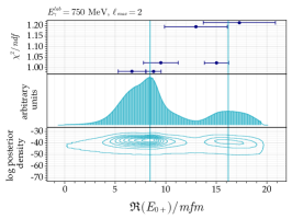
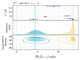
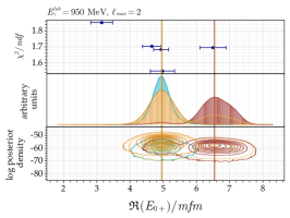
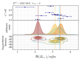
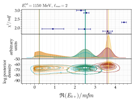
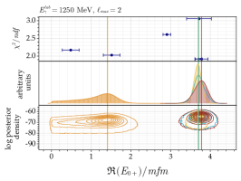
Figure 11: Solutions of the multipole parameter $\real(E_{0+})$ for a truncation order of $\ell_{\text{max}}=2$, for the energy-bins $E^{\text{lab}}_{\gamma}=\quantity[750,850,950,1050,1150,1250]$ MeV. The different parts of the tripartite plots are explained at the beginning of Section VIII.

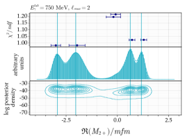
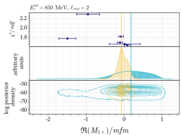
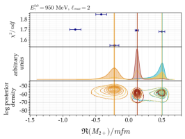
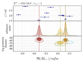
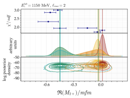
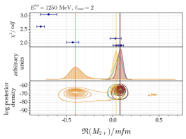
Figure 12: Solutions of the multipole parameter $\real(M_{2+})$ for a truncation order of $\ell_{\text{max}}=2$, for the energy-bins $E^{\text{lab}}_{\gamma}=\quantity[750,850,950,1050,1150,1250]$ MeV. The different parts of the tripartite plots are explained at the beginning of Section VIII.

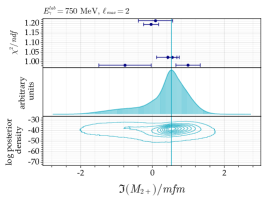
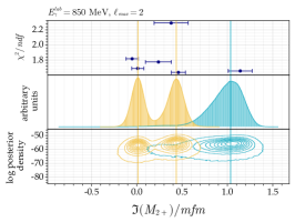
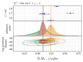
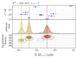
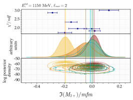
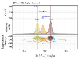
Figure 13: Solutions of the multipole parameter $\imaginary(M_{2+})$ for a truncation order of $\ell_{\text{max}}=2$, for the energy-bins $E^{\text{lab}}_{\gamma}=\quantity[750,850,950,1050,1150,1250]$ MeV. The different parts of the tripartite plots are explained at the beginning of Section VIII.

4)

Within Fig. 14 the solution clusters of the $8\ell_{\text{max}}-1$ multipole parameters are shown as a function of the photon energy $E^{\text{lab}}_{\gamma}$ together with the results of EtaMAID2018 [82], BnGa-2019 [46] and JüBo-2022 [56].

Figure 14: Marginal multipole solutions for the truncation order $\ell_{\text{max}}=2$ for the energy-bins $E^{\text{lab}}_{\gamma}=\quantity[750,850,950,1050,1150,1250]$ MeV. In addition, the multipole parameter predictions from EtaMAID2018 [82] (dashed line), BnGa-2019 [46] (dotted line) and JüBo-2022 [56] (dash-dotted line) are shown as well. The relevance of a solution is represented by a transition from sienna (less relevant) to blue (more relevant) hues. However, for a detailed comparison between the solutions and their relevance to each other, the reader is advised to the tripartite multipole parameter figures in Figs. 11, 12 and 13 and Ref. [72].

For a detailed comparison between the different solution clusters and their relevance to each other, the reader is advised to the tripartite multipole parameter figures in Figs. 11, 12 and 13 and Ref. [72]. In general, the results of this paper are in good agreement with their results. However, for the multipole parameter $\real(E_{0+})$ at $750$ MeV the results of EtaMAID2018, BnGa-2019 and JüBo-2022 are at a value of $\sim 20$ mfm. The data sets of $\eta$-photoproduction (see Section IV) used within this analysis do not emphasize such high values. While the marginal parameter distribution does indeed have a non vanishing probability at $\sim 19$ mfm, it favors values of $\sim 8.5$ mfm. The strength of the multipole $E_{0+}$ near the $\eta p$ production threshold, as seen in EtaMAID2018, BnGa-2019 and JüBo-2022, comes from the dominant $N(1535)1/2^{-}$ resonance, which couples to the $S$-wave $E_{0+}$. The reason for this is probably the conceptual difference between truncated partial-wave and a full partial wave analysis. On the one hand, this information could come from the fact that BnGa-2019 and JüBo-2022 are coupled-channel analyses, which include at the same time multiple different final states [83]. On the other hand, do EtaMAID2018, BnGa-2019 and JüBo-2022 use the $\pi N$ partial-wave amplitudes from SAID [83] as input, in which the $N(1535)1/2^{-}$ resonance is included as well [84]. In contrast, the present analysis is not a coupled-channel analysis and does not use the SAID solutions. In addition, the partial wave analyses use the full available data sets, which, especially for the differential cross section, increase the amount of data in the fits by a large factor. However, a truncated partial-wave analysis is completely model independent, but it is only performed at discrete points in energy, and thus can only use data from selected energy bins. Furthermore, while a dominant $S$-wave $E_{0+}$ leads to for example a nearly constant maximal allowed value of one for the observable $E$ for all angles, the reverse conclusion is not always true. Thus, the observable $E$ can not distinguish between $S$-wave $E_{0+}$ and $P$-wave $M_{1-}$ as both can lead to these maximum values. As can be seen for example in our results for 750 MeV (see Fig. 14), the anticipated strength of $E_{0+}$ has migrated to other multipoles, as for example into $M_{1-}$. Improved statistics of the involved data sets in terms of the angular range or using additional observables in a future analysis, may shift the probability mass of the distribution of $\real(E_{0+})$ at $750$ MeV to the values of the three above-mentioned partial wave models.

5)

In relation to truncation order $\ell_{\text{max}}=1$: if different groups of chains are present for a given energy, these have nearly identical reproduced data distributions, see Fig. 9. Hence, one has to look for additional observables which could resolve the ambiguities. The prediction of observables, which were not utilized in this analysis, can be used for this purpose. Specifically, one is looking for observables for which the different groups of chains give distinct predictions, i.e. unique functional behaviors over the $\cos(\theta)$-range.

Figure 15: Predicted data distributions for the polarization observables $C_{z^{\prime}},H,T_{x^{\prime}},O_{z^{\prime}},L_{x^{\prime}},P,T_{z^{\prime}},O_{x^{\prime}},L_{z^{\prime}}$ and $C_{x^{\prime}}$ for the energy-bins $E^{\text{lab}}_{\gamma}=\quantity[750,850,950,1050,1150,1250]$ MeV, using a truncation order of $\ell_{\text{max}}=2$. In addition, the corresponding values from EtaMAID2018 [82] (dashed line), BnGa-2019 [46] (dotted line) and JüBo-2022 [56] (dash-dotted line) are shown as well.

The utilization of such an observable could resolve the remaining ambiguities. Promising candidates for future measurements of polarization observables are listed in Table 3 and shown in Fig. 15. In particular, the polarization observable $C_{z^{\prime}}$ seems suitable to reduce the ambiguities at all six energy-bins.

Table 3: Promising polarization observable candidates to resolve the ambiguities for truncation order $\ell_{\text{max}}=2$. The corresponding predicted data distributions are shown in Fig. 15.

$E^{\text{lab}}_{\gamma}$ / MeV	Observables
750	$C_{x^{\prime}},C_{z^{\prime}},L_{x^{\prime}},L_{z^{\prime}}$
850	$C_{x^{\prime}},C_{z^{\prime}},L_{x^{\prime}},L_{z^{\prime}},T_{x^{\prime}},T_{z^{\prime}}$
950	$C_{x^{\prime}},C_{z^{\prime}},L_{x^{\prime}},L_{z^{\prime}},T_{z^{\prime}}$
1050	$C_{x^{\prime}},C_{z^{\prime}},L_{x^{\prime}},O_{z^{\prime}},T_{z^{\prime}}$
1150	$C_{z^{\prime}},O_{x^{\prime}},T_{x^{\prime}},T_{z^{\prime}}$
1250	$C_{z^{\prime}}$

VIII.3 Truncation order $\ell_{\text{max}}>2$

In general, the truncation order should be as high as possible, as lower partial waves interfere with higher ones and can create non-negligible contributions. That said, as the truncation order increases so does the number of accidental ambiguities, e.g. $43$ posterior modes were found for $\ell_{\text{max}}=3$ and $1250$ MeV. This leads to a numerical demanding situation for reaching the targeted Markov chain Monte Carlo convergence diagnostics. Through the required, huge number of chains the visual check of clustering becomes challenging as well. Furthermore, the theoretical model with truncation order $\ell_{\text{max}}=2$ is able to describe the data very well, see the reproduced data distributions in Fig. 9. The statistical quality of the used data do not allow to see any F-wave contributions, for example from the $N(1680)5/2^{+}$ [2] resonance at $E^{\text{lab}}_{\gamma}\approx 1035$ MeV.

Due to the mentioned points, the truncation orders $\ell_{\text{max}}>2$ are part of further research and are not shown within this paper.

IX Summary and Outlook

For the first time, Bayesian statistics has been applied to truncated partial-wave analysis. The analysis was performed with the six polarization observables $\sigma_{0},\Sigma,T,E,F$ and $G$ of $\eta$-photoproduction for the energy-bins $E^{\text{lab}}_{\gamma}=[750,850,950,1050,1150,1250]$ MeV and different truncation orders. Hereby, highly multimodal posterior distributions were encountered which enforced adaptations for monitoring the Markov chain Monte Carlo convergence diagnostics.

The analysis itself consisted of a nonlinear model which considered correlations between data points as well as systematic uncertainties. The used data show clear $D$-Wave contributions above $E^{\text{lab}}_{\gamma}=950$ MeV, but are not sensitive to $F$-Wave or higher partial wave contributions.

The results were marginal distributions as well as a posteriori estimates of the electromagnetic multipole parameters. Despite the fact that truncated-partial wave analysis is a simpler, yet model-independent, approach and used significantly less data than a full partial wave analysis, the results of this paper are in good agreement with the results of MAID2018, BnGa-2019 and JüBo-2022.

In addition, predictions for the polarization observables $H$, $P$ as well as of group $\mathcal{BR}$ and $\mathcal{TR}$ were given, which includes previously unmeasured polarization observables. Based on this, promising future measurements could be determined in order to minimize the remaining ambiguities.

In a future study, the role of the prior distribution with regard to resolving the mathematical ambiguities could be investigated. And for even more challenging phase spaces, where the Markov chain Monte Carlo starting values from the maximum a posteriori approach are not in the vicinity of the ’typical set’, one might use the expectation maximization algorithm to determine the marginal posterior modes and use these as starting values.

Appendix A Discrete ambiguities of the analyzed set of six polarization observables

Within this appendix, the discrete partial-wave ambiguities of the six observables $\quantity{\sigma_{0},\check{\Sigma},\check{T},\check{F},\check{G},\check{E}}$ analyzed within this work (cf. Section IV and Table 2) are discussed. It is argued that this specific set is mathematically complete in a truncated partial-wave analysis. As has been demonstrated already in other works (e.g. Ref. [18]), such mathematical considerations can still serve as a useful precursor to analyses of real data.

The following discussion is based on the ’Omelaenko formalism’ [26]. The basic definitions of the sixteen observables in pseudoscalar meson photoproduction, expressed in the transversity basis, are used. The expressions are collected in Table 4.

Table 4: The definition of the sixteen polarization observables in terms of transversity amplitudes $b_{i}$ are displayed. The table is adapted from [21]. The definition of the observables in terms of the required polarization configurations can be found in Table 1.

Observable	Transversity-representation / $\rho$	Type
$\check{\Omega}^{1}=\sigma_{0}$	$\frac{1}{2}\left(\left|b_{1}\right|^{2}+\left|b_{2}\right|^{2}+\left|b_{3}\right|^{2}+\left|b_{4}\right|^{2}\right)$
$\check{\Omega}^{4}=-\check{\Sigma}$	$\frac{1}{2}\left(\left|b_{1}\right|^{2}+\left|b_{2}\right|^{2}-\left|b_{3}\right|^{2}-\left|b_{4}\right|^{2}\right)$	$\mathcal{S}$
$\check{\Omega}^{10}=-\check{T}$	$\frac{1}{2}\left(-\left|b_{1}\right|^{2}+\left|b_{2}\right|^{2}+\left|b_{3}\right|^{2}-\left|b_{4}\right|^{2}\right)$
$\check{\Omega}^{12}=\check{P}$	$\frac{1}{2}\left(-\left|b_{1}\right|^{2}+\left|b_{2}\right|^{2}-\left|b_{3}\right|^{2}+\left|b_{4}\right|^{2}\right)$
$\check{\Omega}^{3}=\check{G}$	$\mathrm{Im}\left[-b_{1}b_{3}^{\ast}-b_{2}b_{4}^{\ast}\right]$
$\check{\Omega}^{5}=\check{H}$	$\mathrm{Re}\left[b_{1}b_{3}^{\ast}-b_{2}b_{4}^{\ast}\right]$	$\mathcal{BT}$
$\check{\Omega}^{9}=-\check{E}$	$\mathrm{Re}\left[b_{1}b_{3}^{\ast}+b_{2}b_{4}^{\ast}\right]$
$\check{\Omega}^{11}=\check{F}$	$\mathrm{Im}\left[b_{1}b_{3}^{\ast}-b_{2}b_{4}^{\ast}\right]$
$\check{\Omega}^{14}=\check{O}_{x^{\prime}}$	$\mathrm{Re}\left[-b_{1}b_{4}^{\ast}+b_{2}b_{3}^{\ast}\right]$
$\check{\Omega}^{7}=-\check{O}_{z^{\prime}}$	$\mathrm{Im}\left[-b_{1}b_{4}^{\ast}-b_{2}b_{3}^{\ast}\right]$	$\mathcal{BR}$
$\check{\Omega}^{16}=-\check{C}_{x^{\prime}}$	$\mathrm{Im}\left[b_{1}b_{4}^{\ast}-b_{2}b_{3}^{\ast}\right]$
$\check{\Omega}^{2}=-\check{C}_{z^{\prime}}$	$\mathrm{Re}\left[b_{1}b_{4}^{\ast}+b_{2}b_{3}^{\ast}\right]$
$\check{\Omega}^{6}=-\check{T}_{x^{\prime}}$	$\mathrm{Re}\left[-b_{1}b_{2}^{\ast}+b_{3}b_{4}^{\ast}\right]$
$\check{\Omega}^{13}=-\check{T}_{z^{\prime}}$	$\mathrm{Im}\left[b_{1}b_{2}^{\ast}-b_{3}b_{4}^{\ast}\right]$	$\mathcal{TR}$
$\check{\Omega}^{8}=\check{L}_{x^{\prime}}$	$\mathrm{Im}\left[-b_{1}b_{2}^{\ast}-b_{3}b_{4}^{\ast}\right]$
$\check{\Omega}^{15}=\check{L}_{z^{\prime}}$	$\mathrm{Re}\left[-b_{1}b_{2}^{\ast}-b_{3}b_{4}^{\ast}\right]$

A.1 Discrete ambiguities of the group $\mathcal{S}$ observables in truncated partial-wave analysis

As is well-known from Omelaenko’s work, in the case of a truncated partial wave analysis with maximum angular momentum $\ell_{\text{max}}$, the four transversity amplitudes can be expressed in terms of linear factorizations:

$$b_{1}\left(\theta\right) =-\hskip 1.0pt\mathcal{C}\hskip 1.0pta_{2L}\hskip 1.0pt\frac{\exp\left(-i\frac{\theta}{2}\right)}{\left(1+t^{2}\right)^{L}}\hskip 1.0pt\prod_{k=1}^{2L}\left(t+\beta_{k}\right)\mathrm{,}$$ (25)

$$\hskip 5.0ptb_{2}\left(\theta\right) =-\hskip 1.0pt\mathcal{C}\hskip 1.0pta_{2L}\hskip 1.0pt\frac{\exp\left(i\frac{\theta}{2}\right)}{\left(1+t^{2}\right)^{L}}\hskip 1.0pt\prod_{k=1}^{2L}\left(t-\beta_{k}\right)\mathrm{,}$$ (26)

$$b_{3}\left(\theta\right) =\mathcal{C}\hskip 1.0pta_{2L}\hskip 1.0pt\frac{\exp\left(-i\frac{\theta}{2}\right)}{\left(1+t^{2}\right)^{L}}\hskip 1.0pt\prod_{k=1}^{2L}\left(t+\alpha_{k}\right)\mathrm{,}\hskip 5.0pt$$ (27)

$$b_{4}\left(\theta\right) =\mathcal{C}\hskip 1.0pta_{2L}\hskip 1.0pt\frac{\exp\left(i\frac{\theta}{2}\right)}{\left(1+t^{2}\right)^{L}}\hskip 1.0pt\prod_{k=1}^{2L}\left(t-\alpha_{k}\right)\mathrm{,}$$ (28)

where $t=\tan\frac{\theta}{2}$ (with the center-of-mass scattering angle $\theta$) and $\quantity{\alpha_{k},\beta_{k}}$ are the Gersten/Omelaenko-roots which are, in essence, equivalent to multipoles.

Furthermore, all permissible solutions have to satisfy Omelaenko’s constraint, i.e. Eq. 10. The solution theory for the case where all four group $\mathcal{S}$ observables have been selected, and thus only ambiguities of the four moduli $\left|b_{1}\right|,\left|b_{2}\right|,\left|b_{3}\right|,\left|b_{4}\right|$ have to be considered, has been worked out at length in Ref. [18]. This solution theory leads to the known complete sets of five (e.g.: $\quantity{\sigma_{0},\check{\Sigma},\check{T},\check{P},\check{F}}$). In the following subsection, the special case where less than four diagonal observables are selected is considered.

A.2 Discrete ambiguities of the three group $\mathcal{S}$ observables $\quantity{\sigma_{0},\Sigma,T}$

The set of observables, used within this work, contains only three simultaneously diagonalized observables ($\sigma_{0},\check{\Sigma},\check{T}$, see Table 4). Therefore, one has to investigate which kinds of discrete ambiguities are allowed by this set of three observables, using the root-formalism described in Section A.1. For this purpose, one can look at the ’minimal’ linear combinations of squared moduli:

$$\sigma_{0}-\check{\Sigma} =2\left(\left|b_{1}\right|^{2}+\left|b_{2}\right|^{2}\right),$$ (29)

$$\sigma_{0}+\check{\Sigma} =2\left(\left|b_{3}\right|^{2}+\left|b_{4}\right|^{2}\right),$$ (30)

$$\sigma_{0}+\check{T} =2\left(\left|b_{1}\right|^{2}+\left|b_{4}\right|^{2}\right),$$ (31)

$$\sigma_{0}-\check{T} =2\left(\left|b_{2}\right|^{2}+\left|b_{3}\right|^{2}\right),$$ (32)

$$-\check{\Sigma}+\check{T} =2\left(\left|b_{1}\right|^{2}-\left|b_{3}\right|^{2}\right),$$ (33)

$$-\check{\Sigma}-\check{T} =2\left(\left|b_{2}\right|^{2}-\left|b_{4}\right|^{2}\right).$$ (34)

Upon reducing the problem to the non-redundant amplitudes $b_{2}$ and $b_{4}$ in the truncated partial-wave analysis (by using $b_{4}(W,\theta)=b_{3}(W,-\theta)$ and $b_{2}(W,\theta)=b_{1}(W,-\theta)$, cf. Eqs. 6 to 9), one obtains:

$$\sigma_{0}-\check{\Sigma} \propto\prod_{k=1}^{2\ell_{\text{max}}}(t+\alpha^{\ast}_{k})(t+\alpha_{k})+\prod_{k=1}^{2\ell_{\text{max}}}(t-\alpha^{\ast}_{k})(t-\alpha_{k}),$$ (35)

$$\sigma_{0}+\check{\Sigma} \propto\prod_{k=1}^{2\ell_{\text{max}}}(t+\beta^{\ast}_{k})(t+\beta_{k})+\prod_{k=1}^{2\ell_{\text{max}}}(t-\beta^{\ast}_{k})(t-\beta_{k}),$$ (36)

$$\sigma_{0}+\check{T} \propto\prod_{k=1}^{2\ell_{\text{max}}}(t+\alpha^{\ast}_{k})(t+\alpha_{k})+\prod_{k=1}^{2\ell_{\text{max}}}(t-\beta^{\ast}_{k})(t-\beta_{k}),$$ (37)

$$\sigma_{0}-\check{T} \propto\prod_{k=1}^{2\ell_{\text{max}}}(t-\alpha^{\ast}_{k})(t-\alpha_{k})+\prod_{k=1}^{2\ell_{\text{max}}}(t+\beta^{\ast}_{k})(t+\beta_{k}),$$ (38)

$$-\check{\Sigma}+\check{T} \propto\prod_{k=1}^{2\ell_{\text{max}}}(t+\alpha^{\ast}_{k})(t+\alpha_{k})-\prod_{k=1}^{2\ell_{\text{max}}}(t+\beta^{\ast}_{k})(t+\beta_{k}),$$ (39)

$$-\check{\Sigma}-\check{T} \propto\prod_{k=1}^{2\ell_{\text{max}}}(t-\alpha^{\ast}_{k})(t-\alpha_{k})-\prod_{k=1}^{2\ell_{\text{max}}}(t-\beta^{\ast}_{k})(t-\beta_{k}).$$ (40)

The problem is now to find out which kinds of discrete ambiguity-transformations, when applied to the roots $\quantity{\alpha_{k},\beta_{k}}$, leave the full set of quantities Eqs. 35 to 40 invariant, while also satisfying the multiplicative constraint Eq. 10. The first set of transformations which comes to mind is given by the well-known double ambiguity:

$$\alpha_{k}\rightarrow\alpha_{k}^{\ast}\hskip 5.0pt\text{and}\hskip 5.0pt\beta_{k}\rightarrow\beta_{k}^{\ast}\hskip 5.0pt\forall k=1,\ldots,2\ell_{max}.$$ (41)

But other transformations may also be possible in addition, since the observable $\check{P}$ is missing from the full diagonalizable set $\quantity{\sigma_{0},\check{\Sigma},\check{T},\check{P}}$. Ideas that one would have to test are for instance exchange symmetries

$$\alpha_{k}\rightarrow\beta_{k}\hskip 5.0pt\text{and}\hskip 5.0pt\beta_{k}\rightarrow\alpha_{k}\hskip 5.0pt\forall k=1,\ldots,2\ell_{max},$$ (42)

sign-changes

$$\alpha_{k}\rightarrow-\alpha_{k}\hskip 5.0pt\text{and}\hskip 5.0pt\beta_{k}\rightarrow-\beta_{k}\hskip 5.0pt\forall k=1,\ldots,2\ell_{max},$$ (43)

or combinations of both

$$\alpha_{k}\rightarrow-\alpha^{\ast}_{k}\hskip 5.0pt\text{and}\hskip 5.0pt\beta_{k}\rightarrow-\beta^{\ast}_{k}\hskip 5.0pt\forall k=1,\ldots,2\ell_{max}.$$ (44)

All of these ideas indeed do not violate the constraint Eq. 10. In case any such additional symmetry of the quantities Eqs. 35 to 40 were found, the next step would be to test which of the remaining three observables $\quantity{F,G,E}$ resolves the symmetry. Neither of the proposed symmetries Eqs. 42, 43 and 44 leaves all the six quantities Eqs. 35 to 40 invariant. It remains to be asked whether such additional symmetries actually exist. In case they do not exist, the discussion would be simplified significantly (since $\check{F}$ and $\check{G}$ in this case already resolve the double ambiguity Eq. 41). Due to information-theoretical reasons, it only seems permissible to simultaneously use three of the quantities from Eqs. 35 to 40, i.e. to use three new quantities obtained via invertible and linear transformations from the three diagonal, initial observables $\quantity{\sigma_{0},\check{\Sigma},\check{T}}$.

As an example, one can select the three quantities given by Eqs. 35, 36 and 37. The full set of discrete ambiguity-transformations, which, when applied to the roots $\quantity{\alpha_{k},\beta_{k}}$, leaves Eqs. 35 and 36 invariant while maintaining the constraint in Eq. 10, is given by the two transformations in Eqs. 41 and 43. Under the exchange symmetry Eq. 42, Eqs. 35 and 36 are transformed into each other and thus are not invariant.

Now considering additionally the quantity in Eq. 37, one can see that while the transformation Eq. 41 leaves this quantity invariant, transformation Eq. 43 does not. This only leaves one possible conclusion, namely that also for the case of only three diagonal observables $\quantity{\sigma_{0},\check{\Sigma},\check{T}}$, or equivalently the three new quantities in Eqs. 35, 36 and 37, the double ambiguity is the only relevant discrete ambiguity of the problem.

The argument given above can be repeated for any other case where a combination of three quantities from the six definitions Eqs. 35 to 40 is taken as a starting point. None of the other starting-combinations is necessary for a proof, since this would give a redundant derivation, with the same outcome.

A.3 Completeness of the set $\quantity{\sigma_{0},\check{\Sigma},\check{T},\check{F},\check{G},\check{E}}$

It has already been shown in Refs. [18, 17] that the observables $\check{F}$ and $\check{G}$ change sign under the double-ambiguity transformation.

All the arguments made up to this point prove that the set $\quantity{\sigma_{0},\check{\Sigma},\check{T},\check{F},\check{G},\check{E}}$ is free of discrete ambiguities in the truncated partial-wave analysis. Assuming furthermore that this set of six observables has no continuous ambiguities, the set is complete.

Appendix B Covered phase space of the used data

The phase-space coverages of the used polarization observable data are illustrated in Fig. 16. For a detailed description of the data see Sections IV and 2. The vertical orange lines correspond to the energy bins of the statistically weakest polarization observable $G$ and indicate by which amount the data set of an other observable has to be shifted to match these energies.

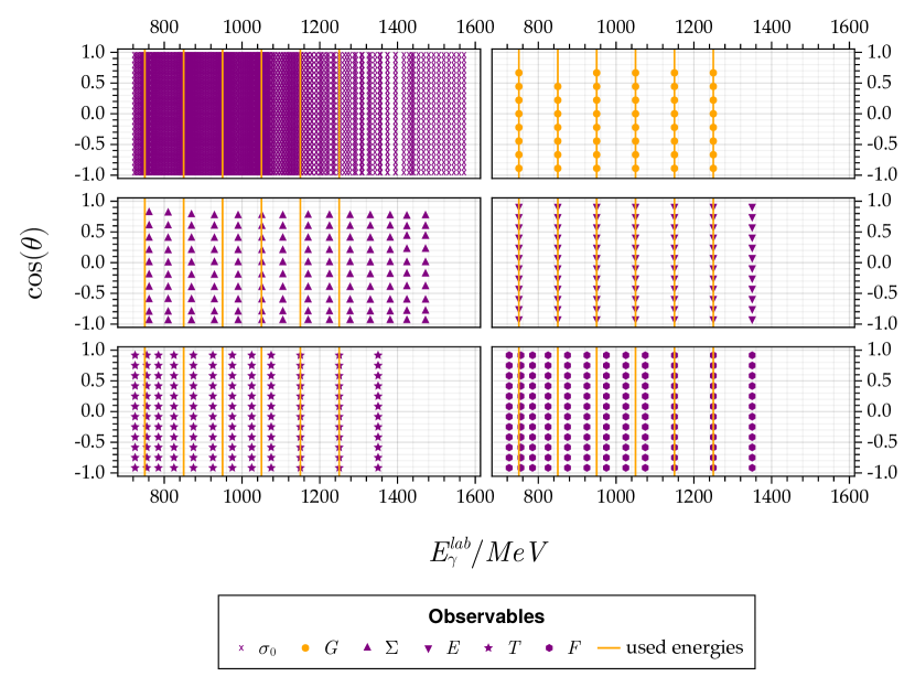
Figure 16: Energy and angular coverage of the six observables $\sigma_{0},\Sigma,G,E,T$ and $F$ [42, 43, 46, 45, 44] which were used for the analysis. The used energies $E^{\text{lab}}_{\gamma}=[750,850,950,1050,1150,1250]$ MeV are determined by the observable $G$.

Appendix C On the correlation of profile functions

The correlation of two random variables $X$ and $Y$ can be calculated using the Pearson correlation coefficient defined as [48]:

$$\mathrm{Corr}(X,Y)=\frac{\mathrm{Cov}(X,Y)}{\sqrt{\mathrm{Var}[X]\mathrm{Var}[Y]}},$$ (45)

with their respective variances $\mathrm{Var}$ and the covariance $\mathrm{Cov}$ between the two random variables. Under the assumption that the dimensionless observables do not have any correlation with each other, the covariance of the unpolarized differential cross-section $\sigma_{0}(W,\theta)$ (denoted with $X$) and a profile function (denoted as $Y^{\prime}=XY$, as $\sigma_{0}(W,\theta)$ was used to calculate the profile function) is:

$$\mathrm{Cov}(X,Y^{\prime}) =\mathrm{E}[XXY]-\mathrm{E}[X]\cdot\mathrm{E}[XY],$$

$$=\quantity(\mathrm{E}[X^{2}]-\mathrm{E}[X]^{2})\cdot\mathrm{E}[Y],$$

$$=\mathrm{Var}[X]\cdot\mathrm{E}[Y].$$ (46)

And similarly for the covariance of one profile function (denoted as $Y^{\prime}=XY$) to another (denoted as $Z^{\prime}=XZ$):

$$\mathrm{Cov}(Y^{\prime},Z^{\prime}) =\mathrm{E}[XYXZ]-\mathrm{E}[XY]\cdot\mathrm{E}[XZ],$$

$$=\quantity(\mathrm{E}[X^{2}]-\mathrm{E}[X]^{2})\cdot\mathrm{E}[Y]\cdot\mathrm{E}[Z],$$

$$=\mathrm{Var}[X]\cdot\mathrm{E}[Y]\cdot\mathrm{E}[Z].$$ (47)

Substituting Eq. 46, and Eq. 47 respectively, into Eq. 45 the correlation for both cases is:

$$\mathrm{Corr}(X,Y^{\prime}) =\sqrt{\frac{\mathrm{Var}[X]}{\mathrm{Var}[Y^{\prime}]}}\cdot\mathrm{E}[Y],$$ (48)

$$\mathrm{Corr}(Y^{\prime},Z^{\prime}) =\frac{\mathrm{Var}[X]}{\sqrt{\mathrm{Var}[Y^{\prime}]\cdot\mathrm{Var}[Z^{\prime}]}}\cdot\mathrm{E}[Y]\cdot\mathrm{E}[Z].$$ (49)

Appendix D Probability distributions for the quotient and product of two Gaussian random-variables

Assuming the original observables to follow a Gaussian probability distribution up to a very good approximation, the result of forming the quotient and/or product is generally non-Gaussian. This appendix collects some basic facts about the quotient- and the product-distribution and considers some limiting cases.

D.1 The quotient distribution: $Z:=X/Y$

Given are two independent, uncorrelated, Gaussian distributed random variables $X$ and $Y$:

$$X\sim\mathcal{N}\left(\mu_{X},\sigma_{X}\right)\mathrm{,}\hskip 5.0ptY\sim\mathcal{N}\left(\mu_{Y},\sigma_{Y}\right)\mathrm{,}$$ (50)

together with the integral defining the probability distribution function of the quotient variable $Z:=X/Y$ [85]:

$$\mathrm{P}_{X/Y}(u) =\int_{-\infty}^{\infty}\differential{x}\int_{-\infty}^{\infty}\differential{y}\delta\left(\frac{x}{y}-u\right)$$

$$\times\frac{\exp\quantity[-\frac{1}{2}\quantity(\frac{(x-\mu_{X})^{2}}{\sigma_{X}^{2}}+\frac{\left(y-\mu_{Y}\right)^{2}}{\sigma_{Y}^{2}})]}{2\pi\sigma_{X}\sigma_{Y}}$$

$$=\int_{-\infty}^{\infty}\differential{y}\left|y\right|\frac{\exp\quantity[-\frac{1}{2}\quantity(\frac{(uy-\mu_{X})^{2}}{\sigma_{X}^{2}}+\frac{\left(y-\mu_{Y}\right)^{2}}{\sigma_{Y}^{2}})]}{2\pi\sigma_{X}\sigma_{Y}}.$$ (51)

Mathematica yields the following result (for positive values of $\sigma_{X}$ and $\sigma_{Y}$):

$$\mathrm{P}_{X/Y}(u) =f_{1}(u)\cdot\left[\sqrt{2}\;f_{2}(u)\;c\right.$$

$$\left.+\sqrt{\pi}\;f_{3}(u)\;\text{erf}\quantity(f_{4}(u))\exp\quantity(f_{4}(u)^{2})\right],$$ (52)

with the declarations:

$$f_{1}(u) :=\frac{\exp(-\frac{1}{2}\quantity(\frac{\mu_{X}^{2}}{\sigma_{X}^{2}}+\frac{\mu_{Y}^{2}}{\sigma_{Y}^{2}}))}{\sqrt{2}\pi f_{2}(u)^{3}},$$ (53)

$$f_{2}(u) :=\sqrt{\sigma_{X}^{2}+\sigma_{Y}^{2}u^{2}},$$ (54)

$$f_{3}(u) :=\mu_{Y}\sigma_{X}^{2}+\mu_{X}\sigma_{Y}^{2}u,$$ (55)

$$f_{4}(u) :=\frac{f_{3}(u)}{\sqrt{2}\;f_{2}(u)\;c},$$ (56)

$$c :=\sigma_{X}\sigma_{Y}$$ (57)

and the error function ’erf’ [86]. In the following, two limiting cases for Eq. 52 are analyzed: first, the vanishing of the expectation values (i.e. $\mu_{X}=\mu_{Y}=0$):

$$\mathrm{P}_{X/Y}(u)=\frac{\sigma_{X}\sigma_{Y}}{\pi\quantity(\sigma_{X}^{2}+\sigma_{Y}^{2}u^{2})}.$$ (58)

This is a result which is known from earlier publications on the quotient distribution, for instance [87].

Second, considering also unit standard-deviations (i.e. $\sigma_{X}=\sigma_{Y}=1$) the result Eq. 58 further simplifies to:

$$\mathrm{P}_{X/Y}(u)=\frac{1}{\pi\left(1+u^{2}\right)}.$$ (59)

This is the well-known Cauchy distribution.

D.2 The product distribution: $Z:=XY$

Similar to Eq. 51 the probability-distribution function for the product of two independent, uncorrelated Gaussian distributed random variables can be written [88]:

$$\mathrm{P}_{XY}(u) =\int_{-\infty}^{\infty}\differential{x}\int_{-\infty}^{\infty}\differential{y}\delta\quantity(xy-u)$$

$$\times\frac{\exp\quantity[-\frac{1}{2}\quantity(\frac{(x-\mu_{X})^{2}}{\sigma_{X}^{2}}+\frac{\left(y-\mu_{Y}\right)^{2}}{\sigma_{Y}^{2}})]}{2\pi\sigma_{X}\sigma_{Y}}.$$ (60)

By introducing an integral-representation for the $\delta$-function

$$\delta\quantity(xy-u)=\int_{-\infty}^{+\infty}\frac{\differential{k}}{2\pi}e^{ik\quantity(xy-u)}=\int_{-\infty}^{+\infty}\frac{\differential{k}}{2\pi}e^{ikxy}e^{-iku},$$ (61)

one can bring Eq. 60 into the following form:

$$\mathrm{P}_{XY}(u)=\int_{-\infty}^{+\infty}\frac{\differential{k}}{2\pi}e^{-iku}F_{k}\quantity[\mu_{X},\sigma_{X};\mu_{Y},\sigma_{Y}],$$ (62)

where

$$F_{k}\quantity[\mu_{X},\sigma_{X};\mu_{Y},\sigma_{Y}]=\int_{-\infty}^{\infty}\differential{x}\int_{-\infty}^{\infty}\differential{y}e^{ikxy}$$

$$\times\frac{\exp\quantity[-\frac{1}{2}\quantity(\frac{(x-\mu_{X})^{2}}{\sigma_{X}^{2}}+\frac{\left(y-\mu_{Y}\right)^{2}}{\sigma_{Y}^{2}})]}{2\pi\sigma_{X}\sigma_{Y}}.$$ (63)

This characteristic function can be solved analytically:

$$F_{k}\quantity[\mu_{X},\sigma_{X};\mu_{Y},\sigma_{Y}]$$

$$=\int_{-\infty}^{\infty}\differential{y}\exp\quantity[-\frac{1}{2}ky\quantity(k\sigma_{X}^{2}y-2i\mu_{X})]\frac{\exp\left[-\frac{\left(y-\mu_{Y}\right)^{2}}{2\sigma_{Y}^{2}}\right]}{\sqrt{2\pi}\sigma_{Y}}$$

$$=\frac{\exp\left[-\frac{k\left(k\mu_{Y}^{2}\sigma_{X}^{2}+k\mu_{X}^{2}\sigma_{Y}^{2}-2i\mu_{X}\mu_{Y}\right)}{2+2k^{2}\sigma_{X}^{2}\sigma_{Y}^{2}}\right]}{\sqrt{1+k^{2}\sigma_{X}^{2}\sigma_{Y}^{2}}}.$$ (64)

The final result has the shape of a Fourier integral:

$$\mathrm{P}_{XY}(u) =\int_{-\infty}^{+\infty}\frac{dk}{2\pi}\exp\left[-iku\right]$$

$$\times\frac{\exp\left[-\frac{k\left(k\mu_{Y}^{2}\sigma_{X}^{2}+k\mu_{X}^{2}\sigma_{Y}^{2}-2i\mu_{X}\mu_{Y}\right)}{2+2k^{2}\sigma_{X}^{2}\sigma_{Y}^{2}}\right]}{\sqrt{1+k^{2}\sigma_{X}^{2}\sigma_{Y}^{2}}}.$$ (65)

In analogy to the quotient distribution, the limiting case $\mu_{X}=\mu_{Y}=0$ shall be analyzed. The Fourier coefficients become:

$$F_{k}\left[0,\sigma_{X};0,\sigma_{Y}\right]=\frac{1}{\sqrt{1+k^{2}\sigma_{X}^{2}\sigma_{Y}^{2}}}.$$ (66)

The result for the product distribution can in this case be written with a modified Bessel function of the second kind $K_{n}(z)$:

$$\mathrm{P}_{XY}(u)=\frac{K_{0}\left(\frac{|u|}{\sigma_{X}\sigma_{Y}}\right)}{\pi\sigma_{X}\sigma_{Y}}.$$ (67)

This is the analogue of Eq. 58 from the case of the quotient distribution. For unit standard deviations, Eq. 67 becomes simply $K_{0}\quantity(\left|u\right|)/\pi$, which is the analogue of Eq. 59.

For the product distribution, especially one limiting case is of interest for this paper, namely where the standard deviation of one random variable almost vanishes (i.e. $\sigma_{Y}\rightarrow 0$). The characteristic function becomes:

$$\lim_{\sigma_{Y}\to 0}F_{k}=\exp\quantity(-\frac{k\quantity(k\mu_{Y}^{2}\sigma_{X}^{2}-2i\mu_{X}\mu_{Y})}{2}).$$ (68)

Substituting Eq. 68 into Eq. 65 and solving the integral gives the result:

$$\mathrm{P}_{XY}(u)=\frac{\exp\quantity(-\frac{\quantity(u-\mu_{X}\mu_{Y})^{2}}{2\mu_{Y}^{2}\sigma_{X}^{2}})}{\sqrt{2\pi}\quantity|\mu_{Y}|\quantity|\sigma_{X}|},$$ (69)

which is indeed a Gaussian probability distribution function. This result is used in Section V.

Appendix E Predictive performance

To allow for the comparison of different models (only possible when each model uses the same data points), a certain measure of model performance is needed. A valid, yet intuitive, choice is its predictive accuracy [36] of a future data point $\tilde{y}_{i}$. This is also known under the name of ’expected out-of-sample log predictive density’ [28] or ’Bayes generalization loss’ [37] and it is defined as [37, 28, 36]:

$$\mathcal{BGL}:= -\mathbb{E}_{\tilde{y}}\quantity[\log\mathbb{E}_{{\bf\it\Theta}}\quantity[p\quantity(\tilde{y}\mid{\bf\it\Theta})]],$$

$$= -\int p_{t}(\tilde{y})\log p(\tilde{y}|{\bf\it y})\differential{\tilde{y}},$$ (70)

with the true probability density function $p_{t}(\tilde{y})$ of the future data [36]. The quantity, defined in Eq. 70 uses a local, proper utility function, as recommended by [89].

However, in a regression problem the quantity $p_{t}(\tilde{y})$ is not known a priori, indeed the overall goal of such an analysis is to gain a deeper understanding of the data generating process. An approximation to Eq. 70 is required, given for example by the Akaike information criterion, deviance information criterion, leave-one-out cross-validation [28] or the widely applicable information criterion [37].

These criteria require the conditional independence of the data points. According to De Finetti’s representation theorem [91, 90], a sequence of random variables is conditional independent on the empirical distribution function, i.e. the sampling distribution of $(y,x)_{i}$, if they are exchangeable [54]. However, as this paper incorporates correlations between the used data points and the off-diagonal elements of the resulting covariance matrix are non-identical, see Section IV, the data pairs $(y,x)_{i}$ are no longer exchangeable. Thus, none of the criteria can be applied to the problem at hand.

Nevertheless, for future analysis that have exchangeable data pairs and involving mathematical ambiguities, it shall be discussed why one should use the widely applicable information criterion.

The widely applicable information criterion was chosen for two reasons. On the one hand, it “is fully Bayesian in that it uses the entire posterior distribution” [36, p. 2] and is an improvement over the Akaike information criterion and deviance information criterion [28, 36]. On the other hand, methods such as K-fold cross validation [36], which require the data to be split into holdout and training sets, should not be used within this analysis. Running the Markov chain Monte Carlo sampling with holdout data points could emphasize one or even produce more mathematical ambiguities, making the estimate of Eq. 70 unreliable. In other words: such a method “has a different problem in that it relies on inference from a smaller subset of the data being close to inference from the full data set, an assumption that is typically but not always true”. [36, p. 16].

The widely applicable information criterion can be calculated by [37]:

$$\mathcal{WAIC}:=\mathcal{BTL}+\mathcal{FV},$$ (71)

with the Bayes training loss [37]:

$$\mathcal{BTL}:=-\frac{1}{N}\sum^{N}_{i=1}\log\mathbb{E}_{{\bf\it\Theta}}\quantity[p(y_{i}\mid{\bf\it\Theta})],$$ (72)

and the functional variance [37]:

$$\mathcal{FV}:=\frac{1}{N}\sum^{N}_{i=1}\mathbb{V}_{{\bf\it\Theta}}\quantity[\log p(y_{i}\mid{\bf\it\Theta})],$$ (73)

with the sample variance $\mathbb{V}_{{\bf\it\Theta}}$. Hence, Eq. 73 serves as a bias term for models comprising more parameters [28].

The quantities in Eqs. 72 and 73 can be calculated from sampled parameter distributions ${\bf\it\Theta}^{s}$ [36]:

$$\widehat{\mathcal{BTL}} =-\frac{1}{N}\sum^{N}_{i=1}\log\quantity(\frac{1}{S}\sum^{S}_{s=1}p(y_{i}\mid{\bf\it\Theta}^{s})),$$ (74)

$$\widehat{\mathcal{FV}} =\frac{1}{N}\sum^{N}_{i=1}\mathbb{V}_{{\bf\it\Theta}^{s}}\quantity[\log p(y_{i}\mid{\bf\it\Theta}^{s})].$$ (75)

The asymptotic equivalence of Bayes generalization loss and $\mathcal{WAIC}$ can be shown to be [37]:

$$\mathbb{E}\quantity[\mathcal{BGL}]=\mathbb{E}\quantity[\mathcal{WAIC}]+\mathcal{O}(\frac{1}{N}),$$ (76)

where $N$ data points were used.

Appendix F Convergence diagnostics

Markov chain Monte Carlo convergence diagnostics for the truncation orders $\ell_{\text{max}}=1$ and $\ell_{\text{max}}=2$ for all analyzed energies are shown in Figs. 17 and 18.

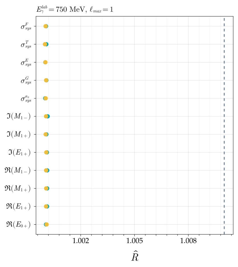
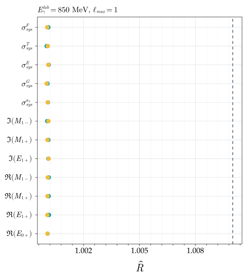
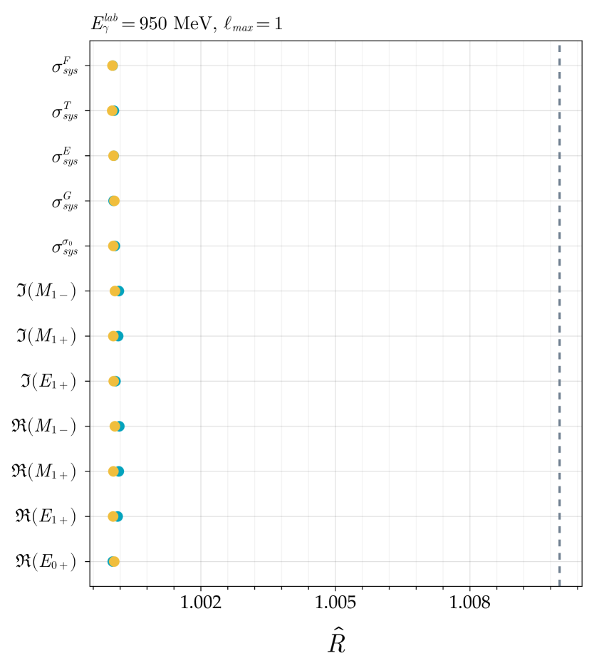
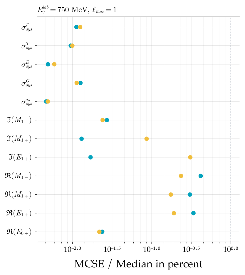
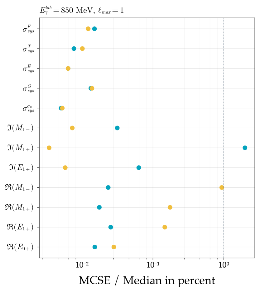
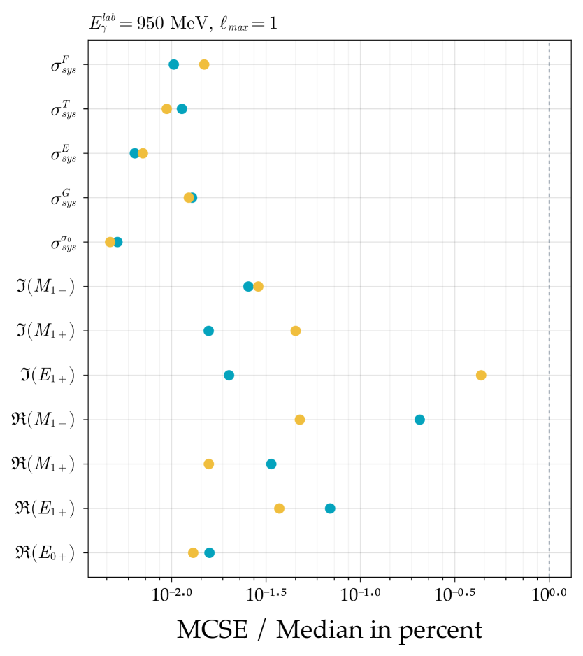
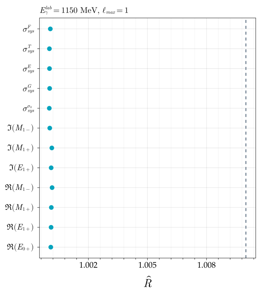
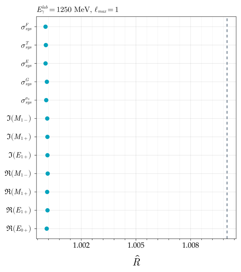
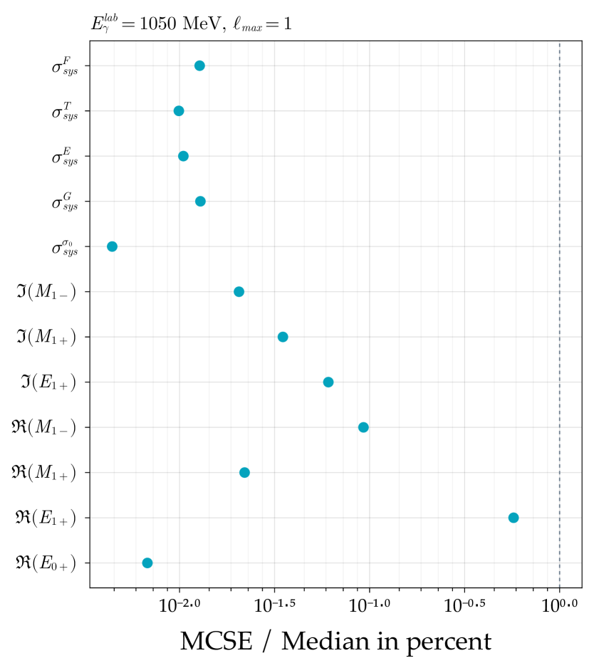
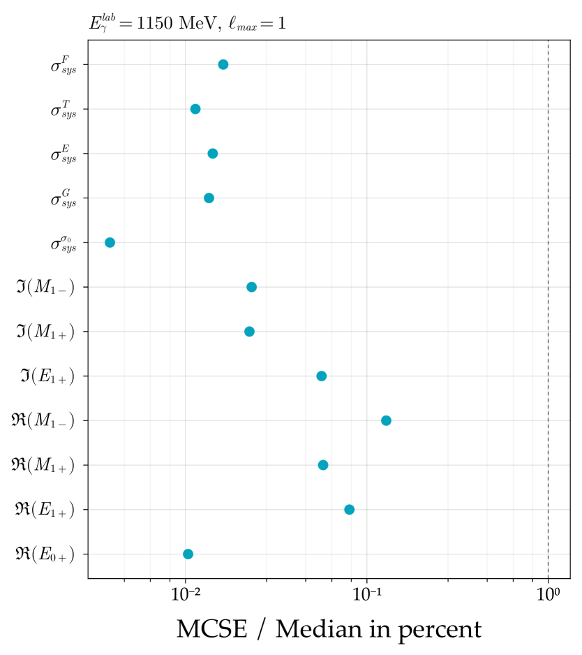
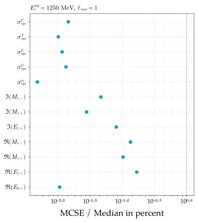
Figure 17: Markov chain Monte Carlo convergence diagnostics for the truncation order $\ell_{\text{max}}=1$. Shown are the potential-scale-reduction statistic $\hat{R}$ (the grey, dashed line indicates the value of 1.01) and the Monte Carlo standard error (MCSE) for the median divided by the median in percent (the grey, dashed line indicates the value of $1\%$).

References

- Thiel et al. [2022] A. Thiel, F. Afzal, and Y. Wunderlich, Light baryon spectroscopy, Progress in Particle and Nuclear Physics 125, 103949 (2022).
- Workman and Others [2022] R. L. Workman and Others (Particle Data Group), Review of Particle Physics, PTEP 2022, 083C01 (2022).
- Haensel [1988] R. Haensel, European synchrotron radiation facility, Nucl. Instrum. Methods Phys. Res., Sect. A.;(Netherlands) 266 (1988).
- Walcher [1990] T. Walcher, The mainz microtron facility mami, Progress in Particle and Nuclear Physics 24, 189 (1990).
- Hillert [2006] W. Hillert, The bonn electron stretcher accelerator elsa: Past and future, in Many Body Structure of Strongly Interacting Systems, edited by H. Arenhövel, H. Backe, D. Drechsel, J. Friedrich, K.-H. Kaiser, and T. Walcher (Springer Berlin Heidelberg, Berlin, Heidelberg, 2006) pp. 139–148.
- Rode et al. [2012] C. Rode, D. Arenius, W. Chronis, D. Kashy, and M. Keesee, Continuous electron beam accelerator facility, Advances in Cryogenic Engineering: Part A & B 35, 275 (2012).
- Yamanaka [1992] C. Yamanaka, Super photon ring-8 and its application to fel, Nuclear Instruments and Methods in Physics Research Section A: Accelerators, Spectrometers, Detectors and Associated Equipment 318, 239 (1992).
- Arndt et al. [2006] R. A. Arndt, W. J. Briscoe, I. I. Strakovsky, and R. L. Workman, Extended partial-wave analysis of scattering data, Phys. Rev. C 74, 045205 (2006).
- Anisovich et al. [2012] A. Anisovich, R. Beck, E. Klempt, V. Nikonov, A. Sarantsev, and U. Thoma, Properties of baryon resonances from a multichannel partial wave analysis, The European Physical Journal A 48, 1 (2012).
- Rönchen et al. [2018] D. Rönchen, M. Döring, and U.-G. Meißner, The impact of photoproduction on the resonance spectrum, The European Physical Journal A 54, 1 (2018).
- Drechsel et al. [1999] D. Drechsel, O. Hanstein, S. Kamalov, and L. Tiator, A unitary isobar model for pion photo- and electroproduction on the proton up to 1 gev, Nuclear Physics A 645, 145 (1999).
- Sato and Lee [1996] T. Sato and T.-S. H. Lee, Meson-exchange model for n scattering and nn reaction, Phys. Rev. C 54, 2660 (1996).
- Švarc et al. [2013] A. Švarc, M. Hadžimehmedović, H. Osmanović, J. Stahov, L. Tiator, and R. L. Workman, Introducing the pietarinen expansion method into the single-channel pole extraction problem, Phys. Rev. C 88, 035206 (2013).
- Ronniger and Metsch [2011] M. Ronniger and B. C. Metsch, Effects of a spin-flavour-dependent interaction on the baryon mass spectrum, The European Physical Journal A 47, 1 (2011).
- Grushin [1989] V. F. Grushin, Photoproduction of Pions on Low-Energy Protons: Complete Experiments and Multipole Analysis, in Photoproduction of Pions on Nucleons and Nuclei, edited by A. A. Komar (Nova Science, New York, 1989) p. 1.
- Tiator [2012] L. Tiator, Towards a model-independent partial wave analysis for pseudoscalar meson photoproduction, in AIP Conference Proceedings, Vol. 1432 (American Institute of Physics, 2012) pp. 162–167.
- Wunderlich et al. [2014] Y. Wunderlich, R. Beck, and L. Tiator, The complete-experiment problem of photoproduction of pseudoscalar mesons in a truncated partial-wave analysis, Phys. Rev. C 89, 055203 (2014).
- Wunderlich [2019] Y. Wunderlich, The complete experiment problem of pseudoscalar meson photoproduction in a truncated partial wave analysis, Ph.D. thesis, Rheinische Friedrich-Wilhelms-Universität Bonn (2019).
- Wunderlich et al. [2017a] Y. Wunderlich, F. Afzal, A. Thiel, and R. Beck, Determining the dominant partial wave contributions from angular distributions of single-and double-polarization observables in pseudoscalar meson photoproduction, The European Physical Journal A 53, 1 (2017a).
- Chew et al. [1957] G. F. Chew, M. L. Goldberger, F. E. Low, and Y. Nambu, Relativistic dispersion relation approach to photomeson production, Phys. Rev. 106, 1345 (1957).
- Chiang and Tabakin [1997] W.-T. Chiang and F. Tabakin, Completeness rules for spin observables in pseudoscalar meson photoproduction, Phys. Rev. C 55, 2054 (1997).
- Nakayama [2019] K. Nakayama, Explicit derivation of the completeness condition in pseudoscalar meson photoproduction, Phys. Rev. C 100, 035208 (2019).
- Wunderlich et al. [2020] Y. Wunderlich, P. Kroenert, F. Afzal, and A. Thiel, Moravcsik’s theorem on complete sets of polarization observables reexamined, Phys. Rev. C 102, 034605 (2020).
- Kroenert et al. [2021] P. Kroenert, Y. Wunderlich, F. Afzal, and A. Thiel, Minimal complete sets for two-pseudoscalar-meson photoproduction, Phys. Rev. C 103, 014607 (2021).
- Ireland [2010] D. G. Ireland, Information content of polarization measurements, Phys. Rev. C 82, 025204 (2010).
- Omelaenko [1981] A. Omelaenko, Ambiguities of the multipole analysis of neutral-pion photoproduction from nucleons, Soviet Journal of Nuclear Physics 34, 406 (1981).
- Bayes [1763] T. Bayes, Lii. an essay towards solving a problem in the doctrine of chances. by the late rev. mr. bayes, frs communicated by mr. price, in a letter to john canton, amfr s, Philosophical transactions of the Royal Society of London , 370 (1763).
- Gelman et al. [2013] A. Gelman, J. B. Carlin, H. S. Stern, D. B. Dunson, A. Vehtari, and D. B. Rubin, Bayesian data analysis (CRC press, 2013).
- Metropolis et al. [1953] N. Metropolis, A. W. Rosenbluth, M. N. Rosenbluth, A. H. Teller, and E. Teller, Equation of state calculations by fast computing machines, The journal of chemical physics 21, 1087 (1953).
- Hastings [1970] W. K. Hastings, Monte Carlo sampling methods using Markov chains and their applications, Biometrika 57, 97 (1970), https://academic.oup.com/biomet/article-pdf/57/1/97/23940249/57-1-97.pdf .
- Duane et al. [1987] S. Duane, A. Kennedy, B. J. Pendleton, and D. Roweth, Hybrid monte carlo, Physics Letters B 195, 216 (1987).
- Neal et al. [2011] R. M. Neal et al., Mcmc using hamiltonian dynamics, Handbook of markov chain monte carlo 2, 2 (2011).
- Geyer [2011] C. J. Geyer, Introduction to markov chain monte carlo, Handbook of Markov chain Monte Carlo 20116022, 45 (2011).
- Gelman and Rubin [1992] A. Gelman and D. B. Rubin, Inference from iterative simulation using multiple sequences, Statistical Science 7, 457 (1992).
- Gelman et al. [2011] A. Gelman, K. Shirley, et al., Inference from simulations and monitoring convergence, Handbook of Markov chain Monte Carlo 6, 163 (2011).
- Vehtari et al. [2017] A. Vehtari, A. Gelman, and J. Gabry, Practical bayesian model evaluation using leave-one-out cross-validation and waic, Statistics and computing 27, 1413 (2017).
- Watanabe [2010] S. Watanabe, Asymptotic equivalence of bayes cross validation and widely applicable information criterion in singular learning theory, Journal of Machine Learning Research 11, 3571 (2010).
- Sandorfi et al. [2011] A. M. Sandorfi, S. Hoblit, H. Kamano, and T.-S. H. Lee, Determining pseudoscalar meson photoproduction amplitudes from complete experiments, Journal of Physics G: Nuclear and Particle Physics 38, 053001 (2011).
- Pichowsky et al. [1996] M. Pichowsky, i. m. c. Şavkli, and F. Tabakin, Polarization observables in vector meson photoproduction, Phys. Rev. C 53, 593 (1996).
- Wunderlich et al. [2017b] Y. Wunderlich, A. Švarc, R. L. Workman, L. Tiator, and R. Beck, Toward an understanding of discrete ambiguities in truncated partial-wave analyses, Phys. Rev. C 96, 065202 (2017b), arXiv:1708.06840 [nucl-th] .
- Workman et al. [2017] R. L. Workman, L. Tiator, Y. Wunderlich, M. Döring, and H. Haberzettl, Amplitude reconstruction from complete photoproduction experiments and truncated partial-wave expansions, Phys. Rev. C 95, 015206 (2017).
- Kashevarov et al. [2017] V. L. Kashevarov, P. Ott, S. Prakhov, P. Adlarson, F. Afzal, Z. Ahmed, C. S. Akondi, J. R. M. Annand, H. J. Arends, R. Beck, A. Braghieri, W. J. Briscoe, F. Cividini, R. Codling, C. Collicott, S. Costanza, A. Denig, E. J. Downie, M. Dieterle, M. I. Ferretti Bondy, L. V. Fil’kov, A. Fix, S. Gardner, S. Garni, D. I. Glazier, D. Glowa, W. Gradl, G. Gurevich, D. J. Hamilton, D. Hornidge, D. Howdle, G. M. Huber, A. Käser, S. Kay, I. Keshelashvili, R. Kondratiev, M. Korolija, B. Krusche, J. Linturi, V. Lisin, K. Livingston, I. J. D. MacGregor, R. MacRae, J. Mancell, D. M. Manley, P. P. Martel, J. C. McGeorge, E. McNicol, D. G. Middleton, R. Miskimen, E. Mornacchi, C. Mullen, A. Mushkarenkov, A. Neiser, M. Oberle, M. Ostrick, P. B. Otte, B. Oussena, D. Paudyal, P. Pedroni, V. V. Polyanski, A. Rajabi, G. Reicherz, J. Robinson, G. Rosner, T. Rostomyan, A. Sarty, D. M. Schott, S. Schumann, C. Sfienti, V. Sokhoyan, K. Spieker, O. Steffen, B. Strandberg, I. I. Strakovsky, T. Strub, I. Supek, M. F. Taragin, A. Thiel, M. Thiel, L. Tiator, A. Thomas, M. Unverzagt, S. Wagner, D. P. Watts, D. Werthmüller, J. Wettig, L. Witthauer, M. Wolfes, R. L. Workman, and L. Zana (A2 Collaboration at MAMI), Study of and photoproduction at mami, Phys. Rev. Lett. 118, 212001 (2017).
- Bartalini et al. [2007] O. Bartalini, V. Bellini, J. Bocquet, P. Calvat, M. Capogni, L. Casano, M. Castoldi, A. d’Angelo, J.-P. Didelez, R. Di Salvo, et al., Measurement of photoproduction on the proton from threshold to 1500 mev, The European Physical Journal A 33, 169 (2007).
- Akondi et al. [2014] C. S. Akondi, J. R. M. Annand, H. J. Arends, R. Beck, A. Bernstein, N. Borisov, A. Braghieri, W. J. Briscoe, S. Cherepnya, C. Collicott, S. Costanza, E. J. Downie, M. Dieterle, A. Fix, L. V. Fil’kov, S. Garni, D. I. Glazier, W. Gradl, G. Gurevich, P. Hall Barrientos, D. Hamilton, D. Hornidge, D. Howdle, G. M. Huber, V. L. Kashevarov, I. Keshelashvili, R. Kondratiev, M. Korolija, B. Krusche, A. Lazarev, V. Lisin, K. Livingston, I. J. D. MacGregor, J. Mancel, D. M. Manley, P. Martel, E. F. McNicoll, W. Meyer, D. Middleton, R. Miskimen, A. Mushkarenkov, B. M. K. Nefkens, A. Neganov, A. Nikolaev, M. Oberle, M. Ostrick, H. Ortega, P. Ott, P. B. Otte, B. Oussena, P. Pedroni, A. Polonski, V. V. Polyanski, S. Prakhov, G. Reicherz, T. Rostomyan, A. Sarty, S. Schumann, O. Steffen, I. I. Strakovsky, T. Strub, I. Supek, L. Tiator, A. Thomas, M. Unverzagt, Y. A. Usov, D. P. Watts, D. Werthmüller, L. Witthauer, and M. Wolfes (A2 Collaboration at MAMI), Measurement of the transverse target and beam-target asymmetries in meson photoproduction at mami, Phys. Rev. Lett. 113, 102001 (2014).
- Afzal [2019] F. N. Afzal, Measurement of the beam and helicity asymmetries in the reactions and , Ph.D. thesis, Rheinische Friedrich-Wilhelms-Universität Bonn (2019).
- Müller et al. [2020] J. Müller, J. Hartmann, M. Grüner, F. Afzal, A. Anisovich, B. Bantes, D. Bayadilov, R. Beck, M. Becker, Y. Beloglazov, A. Berlin, M. Bichow, S. Böse, K.-T. Brinkmann, T. Challand, V. Crede, F. Dietz, M. Dieterle, P. Drexler, H. Dutz, H. Eberhardt, D. Elsner, R. Ewald, K. Fornet-Ponse, S. Friedrich, F. Frommberger, C. Funke, M. Gottschall, A. Gridnev, S. Goertz, E. Gutz, C. Hammann, V. Hannen, J. Hannappel, J. Herick, W. Hillert, P. Hoffmeister, C. Honisch, O. Jahn, T. Jude, I. Jaegle, A. Käser, D. Kaiser, H. Kalinowsky, F. Kalischewski, S. Kammer, I. Keshelashvili, P. Klassen, V. Kleber, F. Klein, E. Klempt, K. Koop, B. Krusche, M. Kube, M. Lang, I. Lopatin, Y. Maghrbi, P. Mahlberg, K. Makonyi, F. Messi, V. Metag, W. Meyer, J. Müllers, M. Nanova, V. Nikonov, D. Novinski, R. Novotny, D. Piontek, G. Reicherz, C. Rosenbaum, T. Rostomyan, B. Roth, A. Sarantsev, C. Schmidt, H. Schmieden, R. Schmitz, T. Seifen, V. Sokhoyan, A. Thiel, U. Thoma, M. Urban, H. van Pee, D. Walther, C. Wendel, U. Wiedner, A. Wilson, A. Winnebeck, and L. Witthauer, New data on with polarized photons and protons and their implications for decays, Physics Letters B 803, 135323 (2020).
- [47] F. Afzal et al. [A2 Collaboration], to be published soon.
- Weisstein [a] E. W. Weisstein, Statistical correlation, From MathWorld–A Wolfram Web Resource. https://mathworld.wolfram.com/StatisticalCorrelation.html (a), Accessed: 2022-05-30.
- Kaiser et al. [2008] K.-H. Kaiser, K. Aulenbacher, O. Chubarov, M. Dehn, H. Euteneuer, F. Hagenbuck, R. Herr, A. Jankowiak, P. Jennewein, H.-J. Kreidel, U. Ludwig-Mertin, M. Negrazus, S. Ratschow, S. Schumann, M. Seidl, G. Stephan, and A. Thomas, The 1.5gev harmonic double-sided microtron at mainz university, Nuclear Instruments and Methods in Physics Research Section A: Accelerators, Spectrometers, Detectors and Associated Equipment 593, 159 (2008).
- Bartalini et al. [2005] O. Bartalini, V. Bellini, J. Bocquet, M. Capogni, L. Casano, M. Castoldi, P. Calvat, A. d’Angelo, R. Di Salvo, A. Fantini, et al., Measurement of photoproduction on the proton from 550 to 1500 mev at graal, The European Physical Journal A-Hadrons and Nuclei 26, 399 (2005).
- Marsaglia [2006] G. Marsaglia, Ratios of normal variables, Journal of Statistical Software 16, 1–10 (2006).
- Jan Hartmann [2017] Jan Hartmann, Measurement of Double Polarization Observables in the Reactions and with the Crystal Barrel/TAPS Experiment at ELSA, Ph.D. thesis, Rheinische Friedrich-Wilhelms-Universität Bonn (2017).
- James and Roos [1975] F. James and M. Roos, Minuit - a system for function minimization and analysis of the parameter errors and correlations, Computer Physics Communications 10, 343 (1975).
- O’Neill [2009] B. O’Neill, Exchangeability, correlation, and bayes’ effect, International Statistical Review 77, 241 (2009), https://onlinelibrary.wiley.com/doi/pdf/10.1111/j.1751-5823.2008.00059.x .
- Döring et al. [2016] M. Döring, J. Revier, D. Rönchen, and R. L. Workman, Correlations of partial waves for multireaction analyses, Phys. Rev. C 93, 065205 (2016).
- Rönchen et al. [2022] D. Rönchen, M. Döring, U.-G. Meißner, and C.-W. Shen, Light baryon resonances from a coupled-channel study including photoproduction (2022), arXiv:2208.00089 [nucl-th] .
- Gelman et al. [2020] A. Gelman, A. Vehtari, D. Simpson, C. C. Margossian, B. Carpenter, Y. Yao, L. Kennedy, J. Gabry, P.-C. Bürkner, and M. Modrák, Bayesian workflow (2020).
- Inc. [2020] W. R. Inc., Mathematica, Version 12.2 (2020), champaign, IL.
- LEVENBERG [1944] K. LEVENBERG, A method for the solution of certain non-linear problems in least squares, Quarterly of Applied Mathematics 2, 164 (1944).
- Marquardt [1963] D. W. Marquardt, An algorithm for least-squares estimation of nonlinear parameters, Journal of the Society for Industrial and Applied Mathematics 11, 431 (1963), https://doi.org/10.1137/0111030 .
- Bezanson et al. [2017] J. Bezanson, A. Edelman, S. Karpinski, and V. B. Shah, Julia: A fresh approach to numerical computing, SIAM Review 59, 65 (2017), https://doi.org/10.1137/141000671 .
- BROYDEN [1970] C. G. BROYDEN, The Convergence of a Class of Double-rank Minimization Algorithms 1. General Considerations, IMA Journal of Applied Mathematics 6, 76 (1970), https://academic.oup.com/imamat/article-pdf/6/1/76/2233756/6-1-76.pdf .
- Fletcher [1970] R. Fletcher, A new approach to variable metric algorithms, The Computer Journal 13, 317 (1970), https://academic.oup.com/comjnl/article-pdf/13/3/317/988678/130317.pdf .
- Goldfarb [1970] D. Goldfarb, A family of variable-metric methods derived by variational means, Math. Comp. 24, 23 (1970).
- Shanno [1970] D. F. Shanno, Conditioning of quasi-Newton methods for function minimization, Math. Comp. 24, 647 (1970).
- Nocedal [1980] J. Nocedal, Updating quasi-Newton matrices with limited storage, Math. Comp. 35, 773 (1980).
- Mogensen and Riseth [2018] P. Mogensen and A. Riseth, Optim: A mathematical optimization package for julia, Journal of Open Source Software 3 (2018).
- Dreschsel and Tiator [1992] D. Dreschsel and L. Tiator, Threshold pion photoproduction on nucleons, Journal of Physics G: Nuclear and Particle Physics 18, 449 (1992).
- Barlow [1993] R. J. Barlow, Statistics: a guide to the use of statistical methods in the physical sciences, Vol. 29 (John Wiley & Sons, 1993).
- Team [2022] S. D. Team, Stan modeling language users guide and reference manual, version 2.28, https://mc-stan.org (2022).
- Hoffman and Gelman [2014] M. D. Hoffman and A. Gelman, The no-u-turn sampler: Adaptively setting path lengths in hamiltonian monte carlo, Journal of Machine Learning Research 15, 1593 (2014).
- [72] See Supplemental Material at https://arxiv.org/src/2305.10367v2/anc/supplement.pdf for all parameter figures and the implementation of the used model within Stan.
- Betancourt [2017] M. Betancourt, A Conceptual Introduction to Hamiltonian Monte Carlo (2017).
- Vehtari et al. [2021] A. Vehtari, A. Gelman, D. Simpson, B. Carpenter, and P.-C. Bürkner, Rank-Normalization, Folding, and Localization: An Improved for Assessing Convergence of MCMC (with Discussion), Bayesian Analysis 16, 667 (2021).
- Zhu et al. [2021] Y.-C. Zhu, Z. Sun, and Q.-L. He, Clustering-based convergence diagnostic for multi-modal identification in parameter estimation of chromatography model with parallel mcmc (2021).
- Jonathan et al. [1999] K. B. Jonathan, J. Goldstein, R. Ramakrishnan, and U. Shaft, When is ”nearest neighbor” meaningful?, in In Int. Conf. on Database Theory (1999) pp. 217–235.
- Graham and Pollak [1971] R. L. Graham and H. O. Pollak, On the addressing problem for loop switching, The Bell system technical journal 50, 2495 (1971).
- Ester et al. [1996] M. Ester, H.-P. Kriegel, J. Sander, X. Xu, et al., A density-based algorithm for discovering clusters in large spatial databases with noise., in kdd, Vol. 96 (1996) pp. 226–231.
- Kolmogorov [1933] A. Kolmogorov, Sulla determinazione empirica di una lgge di distribuzione, Inst. Ital. Attuari, Giorn. 4, 83 (1933).
- Smirnov [1939] N. V. Smirnov, Estimate of deviation between empirical distribution functions in two independent samples, Bulletin Moscow University 2, 3 (1939).
- Scholz and Stephens [1987] F. W. Scholz and M. A. Stephens, K-sample anderson–darling tests, Journal of the American Statistical Association 82, 918 (1987), https://doi.org/10.1080/01621459.1987.10478517 .
- Tiator et al. [2018] L. Tiator, M. Gorchtein, V. L. Kashevarov, K. Nikonov, M. Ostrick, M. Hadžimehmedović, R. Omerović, H. Osmanović, J. Stahov, and A. Švarc, Eta and Etaprime Photoproduction on the Nucleon with the Isobar Model EtaMAID2018, Eur. Phys. J. A 54, 210 (2018), arXiv:1807.04525 [nucl-th] .
- Anisovich et al. [2016] A. Anisovich, R. Beck, M. Döring, M. Gottschall, J. Hartmann, V. Kashevarov, E. Klempt, U.-G. Meißner, V. Nikonov, M. Ostrick, et al., The impact of new polarization data from bonn, mainz and jefferson laboratory on multipoles, The European Physical Journal A 52, 284 (2016).
- Workman et al. [2012] R. L. Workman, R. A. Arndt, W. J. Briscoe, M. W. Paris, and I. I. Strakovsky, Parameterization dependence of -matrix poles and eigenphases from a fit to elastic scattering data, Phys. Rev. C 86, 035202 (2012).
- Weisstein [b] E. W. Weisstein, Normal ratio distribution, From MathWorld–A Wolfram Web Resource. https://mathworld.wolfram.com/NormalRatioDistribution.html (b), Accessed: 2022-09-02.
- Weisstein [c] E. W. Weisstein, Error function, From MathWorld–A Wolfram Web Resource.https://mathworld.wolfram.com/Erf.html (c), Accessed: 2022-09-02.
- Curtiss [1941] J. H. Curtiss, On the Distribution of the Quotient of Two Chance Variables, The Annals of Mathematical Statistics 12, 409 (1941).
- Weisstein [d] E. W. Weisstein, Normal product distribution, From MathWorld–A Wolfram Web Resource. https://mathworld.wolfram.com/NormalProductDistribution.html (d), Accessed: 2022-09-02.
- Bernardo [1979] J. M. Bernardo, Expected information as expected utility, The Annals of Statistics 7, 686 (1979).
- Diaconis and Freedman [1980] P. Diaconis and D. Freedman, Finite exchangeable sequences, The Annals of Probability 8, 745 (1980).
- de Finetti [1992] B. de Finetti, Foresight: Its logical laws, its subjective sources, in Breakthroughs in Statistics: Foundations and Basic Theory, edited by S. Kotz and N. L. Johnson (Springer New York, New York, NY, 1992) pp. 134–174.