Set-Membership Filtering-Based Cooperative State Estimation for Multi-Agent Systems

Abstract

In this article, we focus on the cooperative state estimation problem of a multi-agent system. Each agent is equipped with absolute and relative measurements. The purpose of this research is to make each agent generate its own state estimation with only local measurement information and local communication with neighborhood agents using Set Membership Filter(SMF). To handle this problem, we analyzed centralized SMF framework as a benchmark of distributed SMF and propose a finite-horizon method called OIT-Inspired centralized constrained zonotopic algorithm. Moreover, we put forward a distributed Set Membership Filtering(SMFing) framework and develop a distributed constained zonotopic algorithm. Finally, simulation verified our theoretical results, that our proposed algorithms can effectively estimate the state of each agent.

I Introduction

Recent years, cooperative estimation over sensor networks has received considerable research attention due to its extensive applications in many fields such as target tracking, environmental monitoring and industrial automation [1]. So far theories such as consensus [2] and diffusion strategies [3] have been used for developing filters over sensor networks. From the purpose of cooperative estimation, there are mainly two kinds of problems. The first one is to estimate a common target state by using multiple sensors, and this scene is common in cooperative detection [4]. The second one is each agent utilizes absolute and relative measurements to make the estimation of its own state [5].

For the first kind of cooperative estimation, there are a few articles with set-membership theory to handle this problem, which can be mainly divided into the following two types:

• Ellipsoidal SMF. In [6], a recursive resource-efficient filtering algorithm is proposed to realize distributed estimation in the simultaneous presence of the Round-Robin transmission protocol, the multi-rate mechanism and bounded noises, such that there exists a certain ellipsoid that includes all possible error states at each time instant. Reference [7] considered system with sensor saturation, and derived a sufficient condition for distributed average set-membership filtering algorithm to contain the true state with recursive ellipsoids.

• Polytopic SMF. Reference [8] developed a zonotopic estimation algorithm providing a design of obsever gains to minimize the estimation uncertainties, and proposed a method to reduce the amount of information at each time, which considered the trade-off between communication burden and estimation performance. A distributed zonotopic filter is proposed for robust observation and FDI (Fault Detection and Isolation) of LTV (Linear Time Varying) cyber-physical systems in [9]. The concept of bit-level reduction is introduced to relax the bit-rate requirements to communicate zonotopic sets between agents, and the negociation of data reconciliation strategies to maintain robustness/consistency under potential packet losses is proposed.

However, to the best of our knowledge, few studies paid attention to the second kind of cooperative estimation problem with set-membership filter. Reference [10] defined the parameterized distributed state bounding zonotope for each interconnected system, and proposed an optimization problem to minimize the effect of uncertainties based on the P-radius minimization criterion. Similarly, [11] minimized the intersection zonotopes using an optimization-based method with a series of linear matrix inequalities (LMIs). An on-line method is also discussed for updating the correction matrices method. These two articles are the first propose pioneer of the distributed set-membership estimation problem of systems with inertial interactions. However, relative measurements between neighbourhood agents are not considered in the above mentioned two studies. In the literature, systematic studies of distributed SMFing framework are also neglected. Thus in this article, we study the centralized and distributed set-membership filtering frameworks in the cooperative estimation problem of multi-agent systems with absolute and relative measurements, such that each agent can obtain the estimate of its own state with high accuracy.

The contributions of this paper are summarized as follows:

• To provide a benchmark for distributed set-membership filters, we firstly analyzed the centralized set-membership filtering framework, and put forward a finite horizon constrained zonotopic algorithm. Compared with classical constrained zonotopic algorithm, our algorithm works productively.

• Most importantly, we propose a distributed set-membership filter framework, each can estimate its own state with only local measurements and measurements of its neighbours.

• A decentralized SMF algorithm based on constrained zonotope is then developed with our distributed framework. Finally, simulations examples verified our proposed algorithms.

This paper is organized as follows: Section II gives the system model and the problem description. Section III provides the framework of centralized SMF and our proposed finite-horizon method called OIT-Inspired constrained zonotopic algorithm. In Section IV, we present the framework of distributed SMF, based on this, a distributed constrained zonotopic algorithm is developed. Simulation results are provided to verify our theoretical results in Section V.

Notation: For a sample space $\Omega$, a measurable function $\mathbf{x}:\Omega\to\chi$ from the sample space $\Omega$ to a measurable set $\chi$ is called an uncertain variable. A realization of $\mathbf{x}$ is defined as $\mathbf{x}(\omega)=x$. The range of an uncertain variable is described by its range: $[\![\mathbf{x}]\!]=\{x(\omega):\omega\in\Omega\}$, $\mathbb{R}^{n}$ denotes the $n$- dimensional Euclidean space. The conditional range of $\mathbf{x}$ given $\mathbf{y}=y$ is $[\![\mathbf{x}|y]\!]=\{\mathbf{x}(\omega):\mathbf{y}(\omega)=y,\omega\in\Omega\}=\{\mathbf{x}(\omega):\omega\in\Omega_{\mathbf{y}=y}\}$. A directed graph $\mathcal{G}=(\mathcal{V},\mathcal{E})$ is used to represent system topology. $\mathcal{E}=\{(v_{i},v_{j}):i,j\in\mathcal{V}\}$ is the set of edges which models information flow. In this paper, a set $\overline{\mathcal{N}}_{i}$ is defined as $\overline{\mathcal{N}}_{i}=i\cup\mathcal{N}_{i}$ to denote the union set of the $i$th agent and its in-neighbors, and $q_{i}=|\overline{\mathcal{N}}_{i}|$, where $|\cdot|$ returns the cardinality of a given set. The out-neighborhood of agent $i$ is denoted by $\mathcal{M}_{i}=\{l\in\mathcal{V}:(v_{l},v_{i})\in\mathcal{E}\}$. $\mathbb{N}$ denotes the natural number set, while $\mathbb{N}_{0}$ is the set of positive natural set. $\oplus$ stands for the Minkowski sum. $1_{N}$ denotes a N-length column vector whose each element is $1$.

II System Model and Problem Description

Consider a system composed by $N$ agents, where each agent is identified by a positive integer $i\in\{1,2,\ldots,N\}$. The dynamic of agent $i$ is represented by a discrete-time equation

$$x_{i,k+1}=A_{i}x_{i,k}+B_{i}w_{i,k},\quad i=1,\ldots,N,$$ (1)

where $k\in\mathbb{N}$. As a realization of $\mathbf{x}_{i,k}$, $x_{i,k}\in\mathbb{R}_{i}^{n}$ denotes the state at time instant $k$ for agent $i$, $x_{i,k}\in[\![\mathbf{x}_{i,k}]\!]\subseteq\mathbb{R}_{i}^{n}$; $w_{i,k}$ is the process noise, which is the realization of $\mathbf{w}_{i,k}\in[\![\mathbf{w}_{i,k}]\!]\subseteq\mathbb{R}^{p_{i}}$. $A_{i}\in\mathbb{R}^{n_{i}\times n_{i}}$ stand for the system matrix, while $B_{i}$ is the input matrix with appropriate dimensions.

In this work, we consider two types of measurements, i.e., absolute measurements and relative measurements, which are widely considered in the literature  [12].

Absolute measurement: An absolute measurement refers to agent $i$ takes an observation on its state directly, with an observation equation as the following form:

$$y_{i,k}=C_{i}x_{i,k}+v_{i,k},$$ (2)

where $y_{i,k}\in\mathbb{R}^{m_{i}}$ is the measurement at time instant $k$ for agent $i$. $C_{i}\in\mathbb{R}_{i}^{m_{i}\times n_{i}}$ is the measurement matrix, $v_{i,k}$ is unknown but bounded measurement noise. $v_{i,k}\in[\![\mathbf{v}_{i,k}]\!]$, with $d([\![\mathbf{v}_{i,k}]\!])\leq\overline{v}_{i}$, where $d(\cdot)$ returns the diameter of a set.

Relative measurement: Relative measurements generate the observation with both the state of agent $i$ the in-neighborhood agents $j\in\mathcal{N}_{i}$,

$$z_{i,j,k}=D_{i}(x_{i,k}-x_{j,k})+r_{i,j,k},~{}j\in\mathcal{N}_{i},$$ (3)

where $z_{i,j,k}\in\mathbb{R}^{p_{i}}$ is the measurement at time instant $k$ between agent $i$ and its in-neighborhood agent $j$. $D_{i}\in\mathbb{R}_{i}^{p_{i}\times n_{i}}$ is the measurement matrix. $r_{i,j,k}\in[\![\mathbf{r}_{i,j,k}]\!]$ is the measurement noise, with $d([\![\mathbf{r}_{i,j,k}]\!])\leq\overline{r}_{i,j}$.

In this article, we consider the communication topology is consistent with the time-invariant measurement topology, i.e., $(v_{i},v_{j})\in\mathcal{E}$ implies agent $i$ takes a relative measurement from agent $j$ and receives information from agent $j$ simultaneously.

The aim of this paper is to derive an estimate of uncertain range $S_{i,k}\supseteq[\![\mathbf{x}_{i,k}|y_{0:k},z_{0:k}]\!]$ for each agent $i$ by using all the measurements $y_{i,k}$, $y_{j,k}$ and $z_{i,j,k},~{}j\in\mathcal{N}_{i}$, such that at each instant $k$, $x_{i,k}\in S_{i,k}$.

III Centralized SMFing Framework and Algorithm

In this section, a centralized SMFing framework is presented as the benchmark. Based on this framework, we propose a finite-horizon SMFing constrained zonotopic algorithm with high efficiency. Let $x_{k}=[x_{1,k}^{T},x_{2,k}^{T},\cdots,x_{N,k}^{T}]^{T}$ and $w_{k}=[w_{1,k}^{T},w_{2,k}^{T},\cdots,w_{N,k}^{T}]^{T}$. The system dynamics can be written as follows:

$$x_{k+1} =A_{c}x_{k}+B_{c}w_{k},$$ (4)

where

$$A_{c} =\mathrm{diag}\{A_{1},~{}A_{2},~{}\cdots,~{}A_{N}\},$$ (5)

$$B_{c} =\mathrm{diag}\{B_{1},~{}B_{2},\cdots,~{}B_{N}\}.$$

The augmented form of absolute measurements is

$$y_{k} =[y_{1,k}^{T},y_{2,k}^{T},\cdots,y_{N,k}^{T}]^{T}$$ (6)

$$=C_{c}x_{k}+v_{k},$$

where

$$C_{c} =\mathrm{diag}\{C_{1},~{}C_{2},\cdots,~{}C_{N}\},$$ (7)

$$v_{k} =[v_{1,k}^{T},v_{2,k}^{T},\cdots,v_{N,k}^{T}]^{T}.$$

Since the relative measurements of an agent are related to its in-neighbors, we define $z_{i,k}$ as the all the relative measurements taken by agent $i$, i.e.,

$$z_{i,k} =D_{c}\begin{bmatrix}x_{i,k}-x_{j_{1},k}\\ x_{i,k}-x_{j_{2},k}\\ \vdots\\ x_{i,k}-x_{j_{s},k}\end{bmatrix}+\begin{bmatrix}r_{i,j_{1},k}\\ r_{i,j_{2},k}\\ \vdots\\ r_{i,j_{s},k}\end{bmatrix},\quad j_{1},\cdots,j_{s}\in\mathcal{N}_{i},$$ (8)

where $D_{c}=\mathrm{diag}\{D_{1},~{}D_{2},\cdots,~{}D_{N}\}$.

The relative measurements for all the agents can be written as a compact form $z_{k}=[z_{1,k}^{T},z_{2,k}^{T},\cdots,z_{N,k}^{T}]^{T}$.

Let $Y_{k}=\begin{bmatrix}y_{k}\\ z_{k}\end{bmatrix}$, $r_{i,k}=[r_{i,j_{1},k}^{T},~{}r_{i,j_{2},k}^{T},\cdots,~{}r^{T}_{i,j_{s},k}]^{T}$, $V_{k}=[v_{k}^{T},r_{1,k}^{T},r_{2,k}^{T},\cdots,r_{N,k}^{T}]^{T}$. The augment form of all the measurements can be written as

$$Y_{k} =\begin{bmatrix}C_{c}\\ D_{c}\end{bmatrix}x_{k}+\begin{bmatrix}v_{k}\\ r_{1,k}\\ \vdots\\ r_{N,k}\end{bmatrix}$$ (9)

$$=H_{c}x_{k}+V_{k}.$$

The prediction and update of classical centralized set-membership filter are given as follows:

$$[\![\mathbf{x}_{k}|Y_{0:k-1}]\!]=A_{c}[\![\mathbf{x}_{k-1}|Y_{0:k-1}]\!]\oplus B_{c}[\![\mathbf{w}_{k-1}]\!],$$ (10)

$$[\![\mathbf{x}_{k}|Y_{0:k}]\!]=[\underset{V_{k}\in[\![\mathbf{V}_{k}]\!]}{\bigcup}H^{-1}_{c}(Y_{k}-V_{k})]\cap[\![\mathbf{x}_{k}|Y_{0:k-1}]\!],$$ (11)

where $H^{-1}_{c}(\cdot)$ is the inverse map of $H_{c}(\cdot)$. The uncertain set of agent $i$ solved by centralized set-membership filter is denoted by $S_{i,k}^{c}=\{x_{i,k}:(x_{1,k},x_{2,k},\ldots,x_{N,k})\in[\![\mathbf{x}_{k}|Y_{0:k}]\!]\}$.

A common geometric figure to realize this centralized framework is the extended constrained zonotope, which is defined as follows.

Definition 1.

(Extended Constrained Zonotope [13]) A set $\mathcal{Z}\subseteq\mathbb{R}^{n}$ is an extended constrained zonotope if there exists a quintuple $(G,c,A,b,h)\in\mathbb{R}^{n\times n_{g}}\times\mathbb{R}^{n}\times\mathbb{R}^{n_{c}\times n_{g}}\times\mathbb{R}^{n_{c}}\times[0,\infty]^{n_{g}}$ such that $\mathcal{Z}$ is expressed by

$$\{G\xi+c:A\xi=b,\xi\in\underset{j=1}{\overset{n_{g}}{\prod}}[-h^{(j)},h^{(j)}]\}=:Z(G,c,A,b,h),$$ (12)

where $h^{(j)}$ is the $j$^th component of $h$.

When $h^{(j)}=1,~{}j=1,\cdots,n_{g}$, Definition 1 becomes the classical constrained zonotope in [14]. $\widehat{Z}_{k}^{c}=(G^{c},c^{c},A^{c},b^{c},h^{c})\supseteq[\![x_{k}|Y_{0:k}]\!]$ denotes the centralized posterior uncertain range of the augmented system state at $k$.

Since the centralized method is optimal, we can employ it as a benchmark. However, the complexity will go unbounded as time elapses. To handle this problem, we propose a finite-horizon algorithm (see Algorithm 1) based on the theoretical result of  [13], and we provide a line by line explanation as follows:

Algorithm 1 OIT Inspired Centralized Constrained Zonotopic SMF Algorithm

1:  $\mathbf{Initialization}$. Bounded Constrained zonotope $[\![\mathbf{x}_{0}]\!]\subset\mathbb{R}^{n\times N}$, $\overline{\delta}\geq\mu_{0}-1$.

2:  if $k\leq\overline{\delta}$ then

3:  $\widehat{Z}_{k}^{c}\leftarrow$  (10) and  (11).

4:  else

5:  Set $\widehat{Z}_{k-\overline{\delta}}^{c}=\mathbb{R}^{n\times N}$, with  (10) and  (11), solve $\widehat{Z}_{k}^{c}$.

• Line 1 initializes  Algorithm 1, where the additional parameter $\overline{\delta}$ is the length of time slide window, that a larger $\overline{\delta}$ leads to higher accuracy but increases the complexity. $\mu_{0}$ is the observability index of the augmented system.

• Line 3 is for $k\leq\overline{\delta}$, which is the same as the classical constrained zonotope SMF algorithm [15].

• Line 5 is for $k>\overline{\delta}$, which is a finite-horizon version of Section 5 of  [14] over the time window $[k-\overline{\delta},k]$; it is a simplified version of the OIT inspired constrained zonotopic SMF in [13].

IV Distributed SMFing Framework and Constrained Zonotopic Algorithm

In this section, we propose a framework of distributed set-membership filtering framework that each agent only utilizes its local observation and communication to realized its own high-accuracy state estimation. Based on this framework, we develop a distributed constrained zonotopic SMF algorithm.

IV-A Distributed SMFing Framework

Without loss of generality, we assume agents $j_{1},~{}j_{2},~{}\cdots,~{}j_{s}$ are the in-neighborhood agents of $i$. Let $x_{\overline{\mathcal{N}}_{i},k}=[x^{T}_{i,k},x^{T}_{j_{1},k},\cdots,x_{j_{s},k}^{T}]^{T}$ and $W_{\overline{\mathcal{N}}_{i},k}=[w_{i,k}^{T},w_{j_{1},k}^{T},\cdots,w_{j_{s},k}^{T}]^{T}$ with $W_{\overline{\mathcal{N}}_{i},k}\in[\![\mathbf{W}_{\overline{\mathcal{N}}_{i},k}]\!]$. Then the system dynamic and measurement equation can be written as

$$x_{\overline{\mathcal{N}}_{i},k+1} =\begin{bmatrix}A_{i}&&&\\ &A_{j_{1}}&&\\ &&\ddots&\\ &&&A_{j_{s}}\end{bmatrix}\begin{bmatrix}x_{i,k}\\ x_{j_{1},k}\\ \vdots\\ x_{j_{s},k}\end{bmatrix}$$ (13)

$$+\begin{bmatrix}B_{i}&&&\\ &B_{j_{1}}&&\\ &&\ddots&\\ &&&B_{j_{s}}\end{bmatrix}\begin{bmatrix}w_{i,k}\\ w_{j_{1},k}\\ \vdots\\ w_{j_{s},k}\end{bmatrix}$$

$$=A_{\overline{\mathcal{N}}_{i}}x_{\overline{\mathcal{N}}_{i},k}+B_{\overline{\mathcal{N}}_{i}}W_{\overline{\mathcal{N}}_{i},k},$$

$$Y_{\overline{\mathcal{N}}_{i},k} =\begin{bmatrix}C_{i}x_{i,k}\\ C_{j_{1}}x_{j_{1},k}\\ \vdots\\ C_{j_{s},k}x_{j_{s},k}\\ D_{i}(x_{i,k}-x_{j_{1},k})\\ \vdots\\ D_{i}(x_{i,k}-x_{j_{s},k})\end{bmatrix}+\begin{bmatrix}v_{i,k}\\ v_{j_{1},k}\\ \vdots\\ v_{j_{s},k}\\ r_{i,j_{1},k}\\ \vdots\\ r_{i,j_{s},k}\end{bmatrix}$$ (14)

$$=H_{\overline{\mathcal{N}}_{i},k}x_{\overline{\mathcal{N}}_{i},k}+V_{\overline{\mathcal{N}}_{i},k},$$

where $V_{\overline{\mathcal{N}}_{i},k}=[v_{i,k}^{T},v_{j_{1},k}^{T},\cdots,v_{j_{s},k}^{T},r_{i,j_{1},k}^{T},\cdots,r_{i,j_{s},k}^{T}]^{T}$.

For each agent $i$, $\overline{S}_{i,k}^{d}$ and $S_{i,k}^{d}$ denote the prior and posterior uncertain set at $k$, respectively. The joint uncertain prior and posterior range of $(x_{i},x_{j_{1}},\cdots,x_{j_{s}})$ at $k$ are denoted by $\overline{S}_{i,j_{1},j_{2},\cdots,j_{s},k}^{d}$ and $S_{i,j_{1},j_{2},\cdots,j_{s},k}^{d}$. For convenience, we simplify them as $\overline{S}_{\overline{\mathcal{N}}_{i},k}^{d}$ and $S_{\overline{\mathcal{N}}_{i},k}^{d}$, respectively. The framework of joint distributed set-membership filter is proposed in Algorithm 2 and its detailed explanation is given as follows:

Algorithm 2 Distributed Set-membership Filtering Framework

1:  $\mathbf{Initialization}$. For agent $i$, set the initial joint prior range $S_{i,0}^{d}$

2:  loop

3:     $\mathbf{Prediction}$. Given $S_{i,k-1}^{d}$, each agent’s prior range $\overline{S}_{i,k}^{d}$ is given by

$$\overline{S}_{i,k}^{d}=A_{i}(S_{i,k-1}^{d})\oplus B_{i}[\![\mathbf{w}_{i,k-1}]\!],\quad i=1,2,\cdots,N$$ (15)

4:     Receive $\overline{S}_{j,k}^{d}$ from neighborhood agents The joint prior uncertain range $\overline{S}_{\overline{\mathcal{N}}_{i},k}^{p}=\overline{S}_{i,k}^{d}\times\underset{j\in\mathcal{N}_{i}}{\prod}\overline{S}_{j,k}^{d}$.

5:     $\mathbf{Measurement}$. Take integrated measurements $Y_{\overline{\mathcal{N}}_{i},k}$ .

6:     $\mathbf{Joint~{}Update}$. For $k\in\mathbb{N}_{0}$, given the observation $Y_{\overline{\mathcal{N}}_{i},k}$ the joint posterior set $S_{\overline{\mathcal{N}}_{i},k}^{d}$ is formulated by

$$S_{\overline{\mathcal{N}}_{i},k}^{d}=[\underset{V_{i,k}\in[\![\mathbf{V}_{i,k}]\!]}{\bigcup}H_{\overline{\mathcal{N}}_{i},k}^{-1}(Y_{\overline{\mathcal{N}}_{i},k}-V_{\overline{\mathcal{N}}_{i},k})]\cap\overline{S}_{\overline{\mathcal{N}}_{i},k}^{d}$$ (16)

7:     Receive $S_{l,k}^{d,i}=\{x_{i,k}:(x_{l,k},x_{i,k},\cdots,x_{l_{s},k})\in S_{\overline{\mathcal{N}}_{l},k}^{d}\}$ from $l\in\mathcal{M}_{i}\cap\mathcal{N}_{i}$, $l_{1},\cdots,l_{s}\in\mathcal{N}_{l}$. If $\mathcal{M}_{i}\cap\mathcal{N}_{i}=\emptyset$, $S_{l,k}^{d,i}=R^{n}_{i}$.

8:     $\mathbf{Update~{}Intersection}$. The joint posterior uncertain range of UAV $i$ is formulated by

$$S_{i,k}^{d}=[\underset{l\in\mathcal{M}_{i}\cap\mathcal{N}_{i}}{\cap}S_{l,k}^{d,i}]\cap[\underset{\mathbb{R}_{i}^{n}\times\underset{j\in\mathcal{N}_{i}}{\prod}\mathbb{R}_{j}^{n}\to\mathbb{R}_{i}^{n}}{\mathrm{Proj}}S_{\overline{\mathcal{N}}_{i},k}^{d}]$$ (17)

9:     $k=k+1$;

10:  end loop

• Line 1 initializes the $i$^th agent and its in-neighborhood agents’ joint uncertain range $S_{\overline{\mathcal{N}}_{i},0}^{d}$.

• Line 4 denotes the communication process that transmits the information required in the joint progress.

• Line 6 calculates the joint prediction $\overline{S}_{\overline{\mathcal{N}}_{i},k}^{d}$.

• Line 7-8 formulate $S_{\overline{\mathcal{N}}_{i},k}^{d*}$ using a projection method, where the state estimation can be implemented by computing the intersection of the posterior uncertain range of agents that receive information from $i$.

IV-B Distributed Constrained Zonotopic SMF Algorithm

In this section, we design the distributed SMF algorithm based on constrained zonotope method. To distinguish with the system dynamic matrix $A_{i}$, in this section we use $\overline{A}_{i,k}$ and $\widehat{A}_{i,k}$ to denote prior and posterior in the constrained zonotope expression, respectively. The calculation in each step is highlighted as follows:

(1) Initialization. For agent $i$, set the initial uncertain range as

$$\widehat{Z}_{i,0}^{d}=(\widehat{G}_{i,0}^{d},\widehat{c}_{i,0}^{d},\widehat{A}_{i,0}^{d},\widehat{b}_{i,0}^{d},\widehat{h}_{i,0}^{d})$$ (18)

$$=\{z:z=\widehat{G}_{i,0}^{d}\xi+\widehat{c}_{i,0}^{d},\widehat{A}_{i,0}^{d}\xi=\widehat{b}_{i,0}^{d},\xi\in\underset{t=1}{\overset{n_{g}^{i}}{\prod}}[-\widehat{h}_{i,0}^{d,t},\widehat{h}_{i,0}^{d,t}]\},$$

where $\widehat{h}_{i,0}^{d,t}$ denotes the $t$^th component of $\widehat{h}_{i,0}^{d}$.

(2) Prediction. Given the uncertain range of last instant $\widehat{Z}_{i,k-1}^{d}=(\widehat{G}_{i,k-1}^{d},\widehat{c}_{i,k-1}^{d},\widehat{A}_{i,k-1}^{d},\widehat{b}_{i,k-1}^{d},\widehat{h}_{i,k-1}^{d})$, the prior uncertain range at $k$ is given by

$$\overline{Z}_{i,k}^{d}=(\overline{G}_{i,k}^{d},\overline{c}_{i,k}^{d},\overline{A}_{i,k}^{d},\overline{b}_{i,k}^{d},\overline{h}_{i,k}^{d})$$ (19)

$$=([A_{\overline{\mathcal{N}}_{i}}\overline{G}_{i,k}^{d}\quad B_{i}\overline{G}_{w_{i,k}}],A_{\overline{\mathcal{N}}_{i}}\overline{c}_{i,k}^{d},\begin{bmatrix}\overline{A}_{i,k}^{d}&0\\ 0&\overline{A}_{w_{i,k}}\end{bmatrix},$$

$$\begin{bmatrix}\overline{b}_{i,k}^{d}\\ \overline{b}_{w_{i,k}}\end{bmatrix},\begin{bmatrix}\overline{h}_{i,k}^{d}\\ \overline{h}_{w_{i,k}}\end{bmatrix}).$$

The joint prior uncertain range is given by

$$\overline{Z}_{\overline{\mathcal{N}}_{i},k}^{d}=(\overline{G}_{\overline{\mathcal{N}}_{i},k}^{d},\overline{c}_{\overline{\mathcal{N}}_{i},k}^{d},\overline{A}_{\overline{\mathcal{N}}_{i},k}^{d},\overline{b}_{\overline{\mathcal{N}}_{i},k}^{d},\overline{h}_{\overline{\mathcal{N}}_{i},k}^{d})$$ (20)

$$=(\mathrm{diag}\{\overline{G}_{i,k}^{d},~{}\overline{G}_{j_{1},k}^{d},\cdots,~{}\overline{G}_{j_{s},k}^{d}\},\begin{bmatrix}\overline{c}_{i,k}^{d}\\ \vdots\\ \overline{c}_{j_{s},k}^{d}\end{bmatrix},$$

$$\mathrm{diag}\{\overline{A}_{i,k}^{d},~{}\overline{A}_{j_{1},k}^{d},\cdots,~{}\overline{A}_{j_{s},k}^{d}\},\begin{bmatrix}\overline{b}_{i,k}^{d}\\ \vdots\\ \overline{b}_{j_{s},k}^{d}\end{bmatrix},\begin{bmatrix}\overline{h}_{i,k}^{d}\\ \vdots\\ \overline{h}_{j_{s},k}^{d}\end{bmatrix})$$

(3) Joint update. Given Sample integrated measurements at instant $k$ $y_{i,k}$ and $z_{i,k}$, joint update is given by

$$\widehat{Z}_{\overline{\mathcal{N}}_{i},k}^{d}=(\widehat{G}_{\overline{\mathcal{N}}_{i},k}^{d},\widehat{c}_{\overline{\mathcal{N}}_{i},k}^{d},\widehat{A}_{\overline{\mathcal{N}}_{i},k}^{d},\widehat{b}_{\overline{\mathcal{N}}_{i},k}^{d},\widehat{h}_{\overline{\mathcal{N}}_{i},k}^{d})$$ (21)

$$=([\overline{G}_{\overline{\mathcal{N}}_{i},k}^{p}~{}0],\overline{c}_{\overline{\mathcal{N}}_{i},k}^{d},\begin{bmatrix}\overline{A}_{\overline{\mathcal{N}}_{i},k}^{d}&0\\ 0&\overline{A}_{\overline{\mathcal{N}}_{i},k}^{V_{i}}\\ \overline{G}_{\overline{\mathcal{N}}_{i},k}^{d}&(H_{\overline{\mathcal{N}}_{i},k}^{T}H_{\overline{\mathcal{N}}_{i},k})^{-1}H_{\overline{\mathcal{N}}_{i},k}G_{\overline{\mathcal{N}}_{i},k}^{V_{i}}\end{bmatrix}$$

$$,\begin{bmatrix}\overline{b}_{\overline{\mathcal{N}}_{i},k}^{d}\\ b_{\overline{\mathcal{N}}_{i},k}^{V_{i}}\\ \overline{c}_{\overline{\mathcal{N}}_{i},k}^{d}+(H_{\overline{\mathcal{N}}_{i},k}^{T}H_{\overline{\mathcal{N}}_{i},k})^{-1}H_{\overline{\mathcal{N}}_{i},k}Y_{i,k}\end{bmatrix},\begin{bmatrix}h_{\overline{\mathcal{N}}_{i},k}^{d}\\ h_{\overline{\mathcal{N}}_{i},k}^{V_{i}}\end{bmatrix}).$$

(4) Update intersection. Let $e_{\alpha,u}$ denote a projection matrix to choose the $\alpha$th element from a $u$-length vector, and $E_{\alpha,u}=e_{\alpha,u}\otimes I_{n}$.

The final uncertain range at instant $k$ after update intersection $\widehat{Z}_{i,k}^{d}=(\widehat{G}_{i,k}^{d},\widehat{c}_{i,k}^{d},\widehat{A}_{i,k}^{d},\widehat{b}_{i,k}^{d},\widehat{h}_{i,k}^{d})$ is formulated by

$$\widehat{G}_{i,k}^{d}=[E_{1,q_{i}}\widehat{G}_{\overline{\mathcal{N}}_{i},k}\quad 0],$$ (22)

$$\widehat{c}_{i,k}^{d}=E_{1,q_{i}}\widehat{c}_{\overline{\mathcal{N}}_{i},k},$$ (23)

$$\widehat{A}_{i,k}^{d}=\begin{bmatrix}A_{i,k}^{1,1}\\ A_{i,k}^{2,1}\end{bmatrix},$$ (24)

$$\widehat{b}_{i,k}^{d}=\begin{bmatrix}B_{i,k}^{1,1}\\ B_{i,k}^{2,1}\end{bmatrix},$$ (25)

$$\widehat{h}_{i,k}^{d}=\begin{bmatrix}\widehat{h}^{d}_{\overline{\mathcal{N}}_{i},k}\\ \widehat{h}^{d}_{\overline{\mathcal{N}}_{l_{1}},k}\\ \vdots\\ \widehat{h}^{d}_{\overline{\mathcal{N}}_{l_{s}},k}\end{bmatrix},$$ (26)

where $A_{i,k}^{1,1}=\mathrm{diag}_{l\in M_{i}\cap\overline{\mathcal{N}}_{i}}\{\widehat{A}_{\overline{\mathcal{N}}_{l},k}^{d}\}$ , and $A_{i,k}^{2,1}=[A^{1,1}\quad A^{1,2}]$ is a block matrix composed by $A^{1,1}=\mathbf{1}_{q_{i}}\otimes E_{1,q_{i}}\widehat{G}_{\overline{\mathcal{N}}_{i},k}^{d}$ with $q_{i}=|\overline{\mathcal{N}}_{i}|$; $E_{\alpha_{l},q_{l}}$ denotes the serial number of $i$ in $\overline{\mathcal{N}}_{l}$; $A^{1,2}=\mathrm{diag}_{l\in M_{i}\cap\overline{\mathcal{N}}_{i}}\{E_{\alpha_{l},q_{l}}\widehat{G}_{\overline{\mathcal{N}}_{l},k}^{d}\}$, $B_{i,k}^{1,1}=\begin{bmatrix}\widehat{b}_{\overline{\mathcal{N}}_{i},k}\\ \vdots\\ \widehat{b}_{\overline{\mathcal{N}}_{j_{s}},k}\end{bmatrix}$, and $B_{i,k}^{2,1}=\begin{bmatrix}E_{1}c_{i,j\in\mathcal{N}_{i},k}-E_{\alpha_{1}}c_{l_{1},m\in\mathcal{N}_{l_{1}},k}\\ \vdots\\ E_{1}c_{i,j\in\mathcal{N}_{i},k}-E_{\alpha_{l_{s}}}c_{l_{s},m\in\mathcal{N}_{l_{s}},k}\end{bmatrix}$.

Algorithm 3 Distributed Constrained Zonotopic SMF Algorithm

1:  The initial uncertain range of agent $i$ is given by  (18).

2:  loop

3:     The joint prior uncertain range of agent $i$ and its in-neighborhood agents at instant $k$ is given by  (20).

4:     The joint posterior uncertain range is updated as  (21).

5:     The posterior uncertain range of agent $i$ at instant $k$ is formulated by $\widehat{Z}_{i,k}^{d*}=(\widehat{G}_{i,k}^{d*},\widehat{c}_{i,k}^{d*},\widehat{A}_{i,k}^{d},\widehat{b}_{i,k}^{d},\widehat{h}_{i,k}^{d})$, where each matrix is given in (22) - (26).

6:     Find an interval hull $(\widehat{G}_{i,k}^{d},\widehat{c}_{i,k}^{d})$ such that $\widehat{Z}_{i,k}^{d}=\{z=\widehat{G}_{i,k}^{d}\xi+\widehat{c}_{i,k}^{d}\}\supseteq Z_{i,k}^{d*}$, and the final posterior uncertain range at instant $k$ is $\widehat{Z}_{i,k}^{d}=(\widehat{G}_{i,k}^{d},\widehat{c}_{i,k}^{d},[~{}],[~{}],B_{\infty})$.

7:     $k=k+1$;

8:  end loop

Taking the topology in  Fig. 1 as an example, we explain the update intersection step in Line 6 of  Algorithm 3 as follows:

• The augmented state of UAV2 and its in-neighbourhood UAVs can be written as $\mathbf{x}_{\overline{\mathcal{N}}_{2},k}=[\mathbf{x}_{2,k}^{T},\mathbf{x}_{1,k}^{T},\mathbf{x}_{3,k}^{T},\mathbf{x}_{4,k}^{T}]^{T}$, $q_{2}=|\overline{\mathcal{N}}_{2}|=4$. Clearly, $\mathbf{x}_{2,k}=[I\quad 0\quad 0\quad 0]\mathbf{x}_{\overline{\mathcal{N}}_{2},k}$, the projection matrix is $E_{1,4}=[I\quad 0\quad 0\quad 0]$.

• Notice that UAV2 is also the in-neighbourhood agent of UAV4, which implies $\mathbf{x}_{2,k}$ will appear in the augmented vector $\mathbf{x}_{\overline{\mathcal{N}}_{4},k}$, i.e., $\mathbf{x}_{2,k}=[0\quad I\quad 0][\mathbf{x}_{4,k}^{T},\mathbf{x}^{T}_{2,k},\mathbf{x}^{T}_{3,k}]^{T}$, $q_{4}=|\overline{\mathcal{N}}_{4}|=3$. The corresponding projection matrix is $E_{2,3}=[0\quad I\quad 0]$. The posterior range after update intersection $\widehat{Z}_{2,k}^{d}$ is given by

  $$\widehat{G}_{2,k}^{d}=[E_{1,4}\widehat{G}^{d}_{\overline{\mathcal{N}}_{2},k}\quad 0],$$ (27)

  $$\widehat{c}_{2,k}^{d}=E_{1,4}\widehat{c}^{d}_{\overline{\mathcal{N}}_{2},k},$$

  $$\widehat{A}_{2,k}^{d}=\begin{bmatrix}\widehat{A}^{d}_{\overline{\mathcal{N}}_{2},k}&0\\ 0&\widehat{A}^{d}_{\overline{\mathcal{N}}_{4},k}\\ E_{1,4}\widehat{G}^{d}_{\overline{\mathcal{N}}_{2},k}&-E_{2,3}\widehat{G}^{d}_{\overline{\mathcal{N}}_{4},k}\end{bmatrix},$$

  $$\widehat{b}_{2,k}^{d}=\begin{bmatrix}\widehat{b}^{d}_{\overline{\mathcal{N}}_{2},k}\\ \widehat{b}^{d}_{\overline{\mathcal{N}}_{4},k}\\ E_{1,4}\widehat{c}^{d}_{\overline{\mathcal{N}}_{2},k}-E_{2,3}\widehat{c}^{d}_{\overline{\mathcal{N}}_{4},k}\end{bmatrix},$$

  $$\widehat{h}_{2,k}^{d}=\begin{bmatrix}\widehat{h}^{d}_{\overline{\mathcal{N}}_{2},k}\\ \widehat{h}^{d}_{\overline{\mathcal{N}}_{4},k}\end{bmatrix}.$$

In Line 8, we take an interval hull instead of the precise posterior constrained zonotope for fast calculation.

V Simulation Results

In this section, we consider five UAVs in a 2-D plane, each utilizes absolute and relative measurements to localize its position. Let $x_{i,k}=[p^{T}_{x,i,k},v^{T}_{x,i,k},p^{T}_{y,i,k},v^{T}_{y,i,k}]^{T}$, where $p^{T}_{i,k}$ and $v^{T}_{i,k}$ denote the position and velocity of UAV $i$ at instant $k$, respectively. The parameters are listed as follows:

$$A_{i,k}=\begin{bmatrix}a_{11}&a_{12}\\ a_{21}&a_{22}\end{bmatrix}$$ (28)

with $a_{11}=a_{22}=1+\frac{1}{\omega}(\mathrm{sin}(k+1)\omega T-\mathrm{sin}(k\omega T))$,
$a_{12}=-a_{21}=-\frac{1}{\omega}(\mathrm{cos}(k+1)\omega T-\mathrm{cos}(k\omega T))$, and

$$B_{i}=\begin{bmatrix}\frac{T^{2}}{2}\\ T\end{bmatrix},C_{i}=[1\quad 0],D_{i}=I_{2},\omega=1,T=\frac{\pi}{12}$$ (29)

The topology is shown in  Fig. 1 and the noise constrained zonotope is as follows:

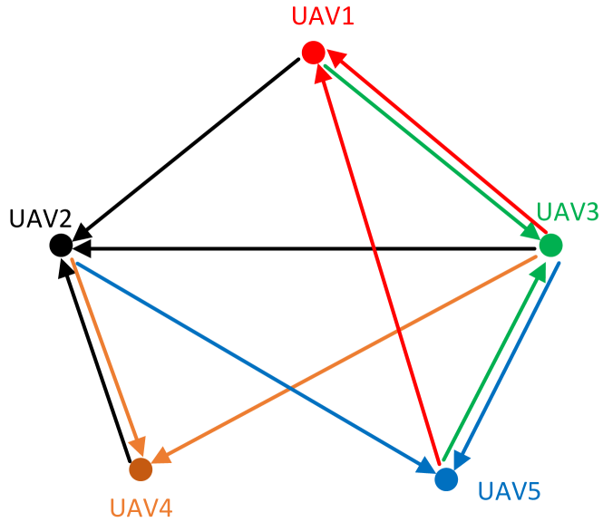
Figure 1: System measurement and communication topology.

$$[\![w_{i,k}]\!]=[\![r_{i,j,k}]\!]=[-1,1]\times[-1,1],[\![v_{i,k}]\!]=[-1,1].$$ (30)

The initial state and its uncertain range are randomly generated by Matlab.

Due to the page limit, we only present the results of UAV 4 and UAV 5. In  Fig. 2, the trajectory of UAV5 is the black line, with the dots representing the real positions at different time steps. The position estimation set in 2-D plane are rectangles. The constrained zonotope generated by OIT-Inspired centralized SMF zonotopic algorithm is presented by pink rectangles, shown as  Fig. 2. The interval hull corresponding to the distributed SMF algorithm is plotted by blue rectangles; see  Fig. 2. At each step, We can see that the constrained zonotope presented by both the OIT centralized algorithm and distributed SMF algorithm contain the real positions of UAV 5, which corroborates the effectiveness of our proposed methods.

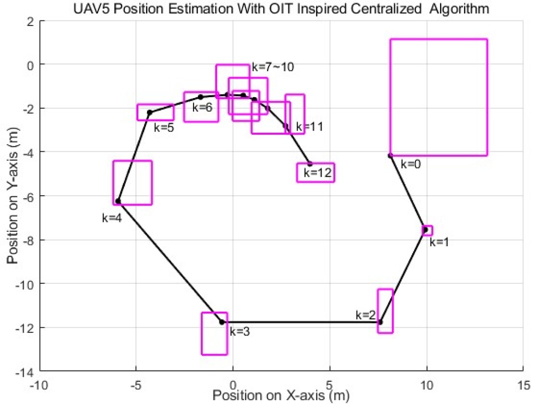
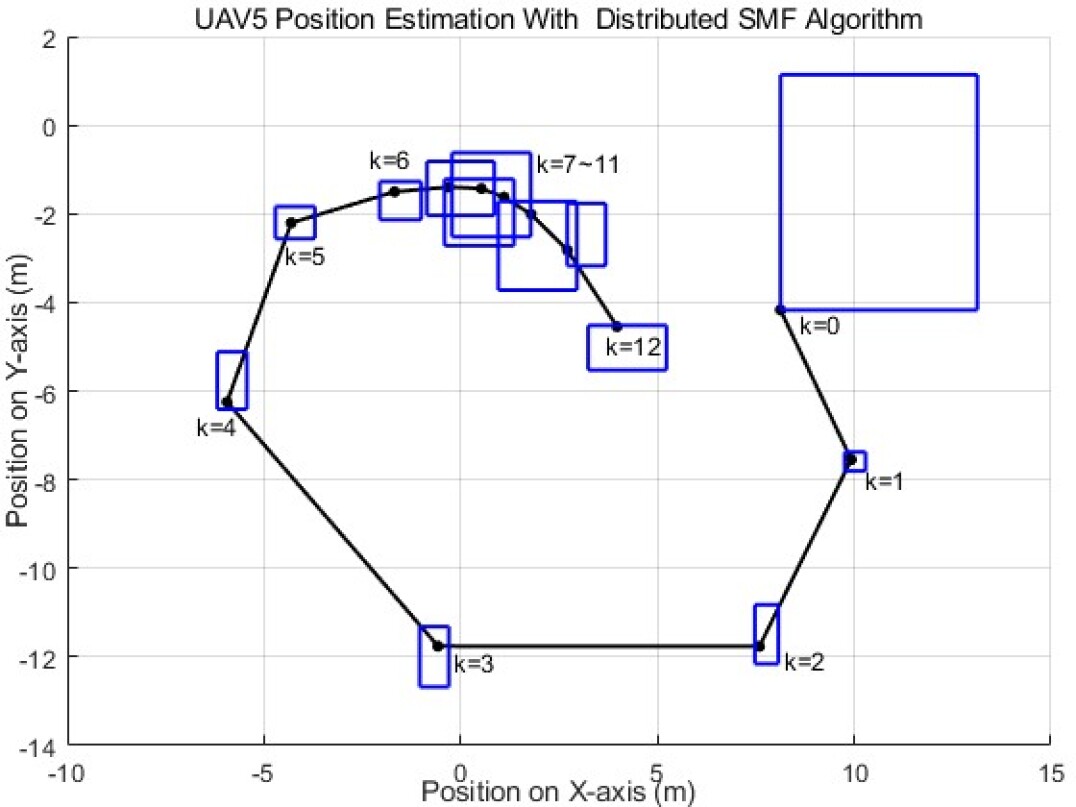
Figure 2: Position estimation of UAV 5 with OIT-Inspired centralized and distributed SMF algorithm. (a)UAV 5 position estimation sketch map with OIT-Inspired centralized constrained zonotopic algorithm. (b) UAV5 position estimation with proposed distributed SMF constrained zonotopic algorithm.

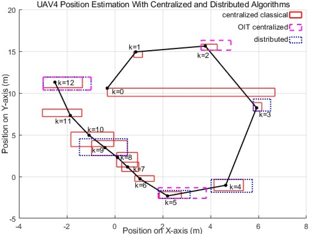
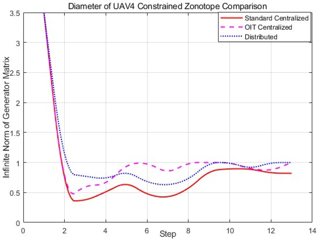
Figure 3: The comparison of standard centralized, OIT-Inspired centralized algorithm and distributed SMF constrained zonotopic algorithm. (a) The constrained zonotope generated by standard centralized SMF algorithm, OIT Inspired centralized algorithm and distributed SMF algorithm simultaneously. (b) The infinite norm of generator matrix $\|G\|_{\infty}$ corresponding to the diameter of uncertain range.

In  Fig. 3, we compare the proposed OIT Inspired centralized algorithm and distributed SMF algorithm with the benchmark (the standard centralized algorithm). The constrained zonotopes generated by standard centralized SMF algorithm each step are presented with red solid line rectangles. The OIT Inspired centralized zonotopes are depicted by pink dash line rectangles. Zonotopic rectangles presented by our proposed distributed algorithm is plotted by blue dotted line. At instant $k=5$ and $k=12$, the three rectangles are labeled together. The red rectangle, corresponding to the standard centralized algorithm, is the smallest among three boxes, which implies both OIT-Inspired method and distributed method have conservativeness. To measure the conservativeness directly, we consider using the diameter of sets, i.e.,

$$d(S)=\underset{s_{1},s_{2}\in S}{\mathrm{sup}}\|s_{1}-s_{2}\|_{\infty}.$$ (31)

For an interval hull in 2-D plane, $d(S)$ is the maximum edge length, which is the twice of the infinite norm of $\widehat{G}$ matrix. Thus in  Fig. 3 we execute comparison of infinite norm of $\widehat{G}$ matrix of the interval hull computed by three algorithms. From  Fig. 3 we can see that the curve corresponding to OIT-Inspired centralized method and distributed method is always above the standard centralized method; This implies our OIT inspired centralized algorithm sacrifice over-estimation accuracy to obtain low complexity, and our distributed SMF method realize distributed structure with low conservativeness.

VI Conclusion

In this paper, we study the state estimation problem of a multi-agent system with absolute and relative measurements. Firstly, we analyzed the centralized SMF framework as the benchmark. To restrict the unlimited complexity increasing in the classical constrained zonotopic algorithm, we develop a finite-horizon version called OIT-Inspired centralized algorithm Secondly, a distributed SMFing framework is presented. Utilizing this framework, each agent can estimate its own state with local measurements and communications with neighbourhood agents. Based on our proposed framework, a distributed SMF zonotopic algorithm is developed. Finally, simulation results indicate that our proposed algorithms are feasible to generate estimation with relatively low conservativeness, and effective facing linear time varying systems.

For future work, we aim to focus on extending our framework to non-linear systems, and consider the stability of our proposed framework.

References

• [1] X. Zhang, S. Li, Z. Lin, and W. Hui, “Range based target localization using a single mobile robot or multiple cooperative mobile robots,” in Proc. of the 10th IEEE Int. Conf. on Control and Automation, 2013.
• [2] R. Olfati-Saber, “Kalman-consensus filter: Optimality, stability, and performance,” in Proc. of the 48h IEEE Conf. on Decision and Control (CDC) and 28th Chinese Control Conf., 2009, pp. 7036–7042.
• [3] M. G. Bruno and S. S. Dias, “A bayesian interpretation of distributed diffusion filtering algorithms,” IEEE Signal Process. Mag., vol. 35, no. 3, pp. 118–123, 2018.
• [4] Y. Zhentao, W. Zhongqing, and L. Peng, “Multi-robot cooperative localization based on maximum consensus cubature kalman filter,” Navigation Positioning and Timing, vol. 9, no. 1, pp. 104–110, 2022.
• [5] D. Viegas, P. Batista, P. Oliveira, and C. Silvestre, “Discrete-time distributed kalman filter design for multi-vehicle systems,” in 2017 Amer. Control Conf. (ACC), 2017, pp. 5538–5543.
• [6] S. Liu, Z. Wang, G. Wei, and M. Li, “Distributed set-membership filtering for multirate systems under the round-robin scheduling over sensor networks,” IEEE Trans. Cybern., vol. 50, no. 5, pp. 1910–1920, 2020.
• [7] H. Zhang, H. Yan, F. Yang, and Q. Chen, “Distributed average filtering for sensor networks with sensor saturation,” IEEE Trans. Control Theory Appl., pp. 887–893, 2013.
• [8] L. Orihuela, P. Millán, S. Roshany-Yamchi, and R. A. García, “Negotiated distributed estimation with guaranteed performance for bandwidth-limited situations,” Automatica, vol. 87, pp. 94–102, 2018.
• [9] A. Combastel, C.;Zolghadri, “Fdi in cyber physical systems: A distributed zonotopic and gaussian kalman filter with bit-level reduction,” IFAC papers Online, pp. 776–783, 2018.
• [10] Y. Wang, T. Alamo, V. Puig, and G. Cembrano, “A distributed set-membership approach based on zonotopes for interconnected systems,” in 2018 IEEE Conf. on Decision and Control (CDC).   IEEE, 2018, pp. 668–673.
• [11] ——, “Distributed zonotopic set-membership state estimation based on optimization methods with partial projection,” IFAC papers online, pp. 4039–4044, 2017.
• [12] W. Li, Y. Jia, and J. Du, “Distributed kalman filter for cooperative localization with integrated measurements,” IEEE Trans. Aerosp. Electron. Syst., vol. 56, no. 4, pp. 3302–3310, 2020.
• [13] Y. C. W. Zhou, “Stability of linear set-membership filters,” 2022.
• [14] J. K. Scott, D. M. Raimondo, G. R. Marseglia, and R. D. Braatz], “Constrained zonotopes: A new tool for set-based estimation and fault detection,” Automatica, 2016.
• [15] Y. Cong, X. Wang, and X. Zhou, “Rethinking the mathematical framework and optimality of set-membership filtering,” IEEE Trans. Autom. Control, vol. PP, no. 99, pp. 1–1, 2021.