Effects of Kaluza-Klein Neutrinos on $R_{D}$ and $R_{D^{*}}$

Abstract

Recent measurements of $R_{D}$ and $R_{D^{*}}$ by the LHCb collaboration show deviations from their respective Standard Model values. These semileptonic $B$ meson decays, associated with $b\rightarrow c\tau\bar{\nu}$ transition, are pointing toward new physics beyond the Standard Model via leptonic flavor universality violation. In this paper, we show that such anomaly can be resolved by the cummulative Kaluza-Klein (KK) modes of singlet right-handed neutrino which propagates in the large extra dimensional space. We found that the number of extra dimension should be 2 to explain $R_{D}$ and $R_{D^{*}}$. We show that both $R_{D}$ and $R_{D^{*}}$ constraint the energy scale $M_{F}$ of this extra dimension which are compatible with the limits from lepton flavor violating tau decays. In contrast, our findings are in tension with the limits coming from the neutrino experiments which set the most stringent lower bound on $M_{F}$. The future measurements of $R_{D^{(*)}}^{exp}$ with reduced uncertainties will exclude this extra dimensional model with right-handed neutrino propagating in the bulk, if the central values stay.

I Introduction

Discrepancies between the Standard Model (SM) predictions and experimental data in the decays of B mesons have gained much attention for years since they may be the hints of new physics beyond the SM, in particular the violations of lepton flavor universality (LFU) in the measurements of $R_{K^{(*)}}$ and $R_{D^{(*)}}$. Even though the updated LHCb measurement LHCb:2022qnv confirmed the consistency with SM predictions in $R_{K}$ and $R_{K^{*}}$ due to the $b\to s$ transitions, the LFU violation remains about $3\sigma$ away from the SM expectations in $b\rightarrow c\tau\bar{\nu}_{\tau}$ transition in the $R_{D}$ and $R_{D^{*}}$ measurements.

The definition of $R_{D^{(*)}}$ is given as

$$R_{D^{(*)}}=\dfrac{Br(B\rightarrow D^{(*)}\tau\bar{\nu}_{\tau})}{[(Br(B\rightarrow D^{(*)}e\bar{\nu}_{e}+Br(B\rightarrow D^{(*)}\mu\bar{\nu}_{\mu}))/2]},$$ (1)

which is independent of $|V_{cb}|$ and also of the $B\to D^{(*)}$ form factor to a large extent HFLAV:2022pwe . A newly calculated world average Iguro using the data from Belle, BaBar, and LHCb collaborations in 2022 obtained $R_{D}^{ave}=0.358\pm 0.027$ and $R_{D^{*}}^{ave}=0.285\pm 0.013$. The SM predictions of the branching ratios $R_{D}^{SM}$ and $R_{D^{*}}^{SM}$ are $0.298\pm 0.004$ and $0.254\pm 0.005$ HFLAV:2022pwe , respectively, which are clearly smaller than the measurements. After incorporating all the recent developments in $B\rightarrow D^{(*)}$ that include form factors for predicting $R_{D^{(*)}}^{SM}$, the largest pull of the combined new world average is $4.1\sigma$ from SM predictions Iguro . Furthermore, even the most updated results of LHCb HFLAV:2023prelim using the data collected in 2015 and 2016 are included, the global picture of the combined new world average does not change. And this corresponds to the most recent combined world average $R_{D}^{ave}=0.356\pm 0.029$ and $R_{D^{*}}^{ave}=0.284\pm 0.013$. For this large deviation, the new physics effect could be comparable to the tree-level SM contributions, therefore many models have been proposed, such as introducing leptoquarks Hiller:2021pul , or new colorless vector $W^{\prime}$ Megias:2017ove , or scalar particles Tanaka:1994ay as tree-level mediators.

In this work, we study a large extra-dimensional model in which three generations of right-handed neutrinos propagate in the bulk Strumia:2000 . As a result of the compactification of these fields, active neutrinos become massive and eventually mix with KK neutrinos due to the mass matrix diagonalization process. Concerning $R_{D}^{(*)}$, it is important to note that SM tree-level semileptonic processes with $W^{\pm}$ as mediators preserved the LFU in the SM. With the existence of KK neutrinos, there may be additional decay channels for $b$ decays into $c$ and KK neutrinos, $b\rightarrow c\ell\bar{\nu}_{\ell}^{KK}$, if KK neutrinos are light enough. Furthermore, if $b\rightarrow c\tau\bar{\nu}_{\tau}^{KK}$ decay width is much lager than $b\rightarrow ce\bar{\nu}_{e}^{KK}$ and $b\rightarrow c\mu\bar{\nu}_{\mu}^{KK}$, the $R_{D^{(*)}}$ would be larger than the SM prediction, and this is the case we consider in this study. Namely, new physics contributes to $R_{D}^{(*)}$ from the cumulative effects of $\tau$ neutrino KK modes in $b\rightarrow c\tau\bar{\nu}_{\tau}^{KK}$ transition as a tree-level process via $W^{\pm}$ exchange.

The following is how the paper is structured: we briefly discuss the extra-dimensional KK model described by Strumia:2000 in section II. Then in section III, we calculate the decay width $\Gamma(B\rightarrow D\tau\bar{\nu}_{\tau}^{KK})$ in a tree-level process to determine the total contributions of the KK neutrinos to $R_{D^{(*)}}$ measurements. Section IV discusses the constraints we consider for the lower limits of fundamental scale $M_{F}$ of extra dimension. In addition to this part, the results of a combined analysis of several neutrino experiments performed in Forero:2022skg to confront the upper bound of the Large Extra Dimension (LED) size $R$ has been implemented. From Forero:2022skg , the upper bound for $R$ at $90\%$ confidence level (C.L.) is $R<0.20\,\mu m$ for normal ordering (NO) and $R<0.10\,\mu m$ for inverted ordering (IO). Finally, in section V we present our conclusions.

II Model

In this section, we briefly review a model in the extra-dimensional framework, where three right-handed neutrinos are introduced and able to propagate in the bulk, while all the SM particles are on the brane Strumia:2000 .

The effective action of such interaction is given as Strumia:2000

$$S=\int d^{4}xdy[\bar{\Psi_{i}}\Gamma_{A}i\partial^{A}\Psi_{i}]+\int d^{4}x[\bar{\nu_{i}}i\not{\partial}\nu_{i}+\nu_{i}\lambda_{ij}\psi_{j}(x^{\mu},0)H+h.c.]\,,$$ (2)

where $A=0,1,2,3,4$, $\Psi_{i}(x,y)$ and $\nu_{i}$ with $i=1,2,3$ are respectively the right-handed neutrino and active neutrino fields, $H$ is the 4D Higgs doublet, and $\lambda$ is the matrix of Yukawa couplings. The right-handed neutrino fields can be written as

$$\Psi_{j}(x,y)=\begin{pmatrix}\psi_{j}(x,y)\\ \bar{\psi}_{j}^{c}(x,y)\end{pmatrix}\,,$$ (3)

such that $\psi_{j}$ and $\bar{\psi}_{j}^{c}$ are two-component Weyl spinors in five dimensions. Here, we denote $x\equiv x^{\mu}$ as the four-vector with $\mu=0,1,2,3$, where $x^{0}$ is the time coordinate and $x^{i}$ are the spatial coordinates for each $i=1,2,3$. The extra-dimensional coordinates are represented by $y\equiv y^{k}$, where $k=1,2,...,\delta$ with $\delta$ the number of extra dimensions. Note that the fundamental scale $M_{F}$ is related to the Planck scale $M_{p}\simeq 10^{19}$ GeV by $M_{F}^{\delta+2}\simeq M_{P}^{2}R^{-\delta}$. Suppose $\Psi_{j}(x,y)$ are $2\pi R$-periodic on variable $y$ then we can express its components into Fourier modes as

$$\psi_{j}(x,y)=\frac{1}{\sqrt{2\pi R}}\sum_{n=-\infty}^{+\infty}\psi_{j}^{(n)}(x)\exp(\frac{iny}{R})\,,$$ (4)

$$\psi_{j}^{c}(x,y)=\frac{1}{\sqrt{2\pi R}}\sum_{n=-\infty}^{+\infty}\psi_{j}^{(n)c}(x)\exp(\frac{iny}{R})\,.$$ (5)

With a redefinition of the standard left-handed neutrinos $\nu_{i}$ with its neutrino flavor eigenstates, the relation

$$\nu_{\alpha,L}^{f}=\sum_{i=1,2,3}V_{\alpha i}\nu_{i},\>\>\>\>\>\>\>\>\alpha=e,\mu,\tau.$$ (6)

and the compactification in coordinate $y$ on a circle of radius $R$, the action  (2), after spontaneous symmetry breaking, will give $S=\int\mathcal{L}d^{4}x$ Strumia:2000 , where

$$\mathcal{L}=\sum_{i=1,2,3}\left(\bar{\nu}_{i}i\not{\partial}\nu_{i}+\sum_{n=-\infty}^{+\infty}\Big{[}\bar{\psi}_{i}^{(n)}i\not{\partial}\psi_{i}^{(n)}+\bar{\psi}_{i}^{(n)c}i\not{\partial}\psi_{i}^{(n)c}+m_{i}\nu_{i}\psi_{i}^{(n)}\Big{]}+\sum_{n=1}^{+\infty}\dfrac{n}{R}(\psi_{i}^{(n)}\psi_{i}^{(n)c}-\psi_{i}^{(-n)}\psi_{i}^{(-n)c})+h.c.\right)$$ (7)

such that $m_{i}=\dfrac{M_{F}}{M_{P}}\dfrac{h_{i}v}{\sqrt{2}}$ as in Ioannisian:1999cw , with $h_{i}$ as the corresponding Yukawa coupling for $i=e,\mu,\tau$. It is important to note that $m_{i}$ is suppressed by a volume factor $\dfrac{M_{F}}{M_{P}}$ of the extra compactified dimensions Hamed ; Dienes . Finally the relevant mass terms in the action is given by

$$\mathcal{L}_{mass}^{KK}=\sum_{i,j=1}^{3}N_{Li}^{T}M_{ij}N_{Rj}+h.c.\,,$$ (8)

with KK index being suppressed, and the mass matrix is given by

$$M=\begin{pmatrix}m_{i}&\sqrt{2}m_{i}&\sqrt{2}m_{i}&...\\ 0&\frac{1}{R}&0&...\\ 0&0&\frac{2}{R}&...\\ \vdots&\vdots&\vdots&\ddots\\ \end{pmatrix}\,.$$ (9)

The corresponding basis vectors for this mass matrix are

$$N_{Li}=\begin{pmatrix}\nu\\ \nu_{nL}\\ \end{pmatrix}_{i},\>\>\>\>\>\textrm{and}\>\>\>\>\>N_{Ri}=\begin{pmatrix}\nu_{R}\\ \nu_{nR}\\ \end{pmatrix}_{i}\,,$$ (10)

where we have redefined the fields as Strumia:2000

$$\nu_{nR.i}=\dfrac{1}{\sqrt{2}}(\psi_{i}^{(n)}+\psi_{i}^{(-n)}),\>\>\>\>\>\nu_{(n)L,i}=\dfrac{1}{\sqrt{2}}(\psi_{i}^{(n)c}+\psi_{i}^{(-n)c})\>\>\>\>\>\textrm{for}\>\>\>\>\>n\geq 1\>\>\>\>\>\textrm{and}\>\>\>\>\nu_{R}=\psi_{i}^{0}.$$ (11)

We diagonalize the matrix $MM^{T}$ for each generation $i$ using a unitary matrix $U^{(i)}$ to obtain the square of the masses of the mass eigenstates. Let’s call the eigenvalues of $MM^{T}$ to be $\dfrac{\lambda_{i}^{(n)2}}{R^{2}}$ which satisfies Strumia:2000

$$\lambda_{i}^{(n)2}-\pi\lambda_{i}^{(n)}\xi_{i}^{2}\cot\pi\lambda_{i}^{(n)}=0\,,$$ (12)

for $n\geq 0$ and $\xi_{i}=m_{i}R$ with $i=e,~{}\mu,~{}\tau$.

Following Ioannisian:1999cw ; Langacker the mixing component of KK neutrinos for active neutrinos can be written as

$$\Xi^{(i)}\equiv\big{(}\dfrac{U_{01}^{(i)}}{U_{00}^{(i)}},\dfrac{U_{02}^{(i)}}{U_{00}^{(i)}},\dfrac{U_{03}^{(i)}}{U_{00}^{(i)}},...\big{)}\,.$$ (13)

As shown in Strumia:2000 ; Dienes ; Dvali ; Mohapatra by setting $\xi_{i}=m_{i}R$ we obtain

$$U_{0n}^{(i)2}=\dfrac{2}{1+\pi^{2}\xi_{i}^{2}+\dfrac{\lambda_{i}^{(n)2}}{\xi_{i}^{2}}}\,.$$ (14)

In the case of $\xi_{i}<<1$ the approximation $\lambda_{n}^{(i)}\approx n$ for $n>0$ gives

$$U_{0n}^{(i)2}\approx\dfrac{2\xi_{i}^{2}}{\xi_{i}^{2}+n^{2}}.$$ (15)

Consequently, for $n=0$, $\lambda_{0}^{(i)}$ is approximately equal to $\xi_{i}$ which yields $U_{00}^{(i)2}\approx 1$. Therefore it can be easily checked in equation (13) that

$$\Xi^{(i)}\approx(U_{01}^{(i)},U_{02}^{(i)},U_{03}^{(i)},...).$$ (16)

The following is the relevant interaction Lagrangian involving the neutrino mass eigenstates $\nu_{l}$ and $\chi^{(n)}$, the charged leptons $l$, together with the weak bosons $W^{\pm}$, and their corresponding Goldstone bosons $G^{\pm}$ given by Schechter

$$\mathcal{L}_{W^{\pm}}^{int} =-\dfrac{g_{w}}{\sqrt{2}}W^{-\mu}\sum_{l=e,\mu,\tau}\Big{(}B_{l\nu_{l}}\bar{l}\gamma_{\mu}P_{L}\nu_{l}+\sum_{n=-\infty}^{\infty}B_{l,n}\bar{l}\gamma_{\mu}P_{L}\chi^{(n)}+h.c.\Big{)}\,,$$

$$\mathcal{L}_{G^{\pm}}^{int} =-\dfrac{g_{w}}{\sqrt{2}M_{W}}G^{-}\sum_{l=e,\mu,\tau}\Big{[}B_{l\nu_{l}}m_{l}\bar{l}P_{L}\nu_{l}+\sum_{n=-\infty}^{\infty}B_{l,n}\bar{l}\big{(}m_{l}P_{L}-m_{(n)}P_{R}\big{)}\chi^{(n)}+h.c.\Big{]}\,,$$ (17)

where $g_{w}$ is the weak coupling constant and $P_{R,L}=\dfrac{1\pm\gamma_{5}}{2}$ are the chirality projection operators. Here $m_{(n)}$ and $m_{l}$ represent the masses of KK neutrinos and charged leptons respectively. Also the expressions for the elements of the matrix $B$ are given in Ioannisian:1999cw

$$B_{l,n}=\sum_{i=e,\mu,\tau}V_{li}^{l}U_{i,n}^{\nu}\,,\qquad B_{l\nu_{k}}=\sum_{i=e,\mu,\tau}V_{li}^{l}U_{ik}^{\nu}\quad\textrm{for each}\>\>k=e,\mu,\tau\,,$$ (18)

where the matrix $V^{l}$ diagonalizes the charged lepton mass matrix Indeed, the KK neutrino mixing parameters emphasized in Ioannisian:1999cw ; Langacker ; jcaban are

$$(s_{L}^{\nu_{i}})^{2}=\sum_{n=1}^{+\infty}{|B_{l,n}|^{2}}\approx\Xi^{(i)}\Xi^{(i)T}\approx\sum_{n=1}^{\infty}{U_{0n}^{(i)2}}.$$ (19)

The discrete summation including all of the KK modes can be written into continuous integration over all of its energy scale $E$ as a prescription of Ioannisian:1999cw ; jcaban

$$\sum_{n=1}^{\infty}\longrightarrow S_{\delta}R^{\delta}\int_{\frac{1}{R}}^{M_{F}}E^{\delta-1}dE\,,$$ (20)

with $M_{F}$ as the ultraviolet (UV) cut-off, $R$ is the radius of the extra dimension, and $S_{\delta}=2\pi^{\delta/2}/\Gamma(\frac{\delta}{2})$ to be the surface area of the unit sphere in $\delta$ dimensions. As a result, the mixings can be expressed as

$$(s_{L}^{\nu_{i}})^{2}\approx\begin{cases}\dfrac{\pi h_{i}^{2}v^{2}}{M_{F}^{2}}\ln\Big{[}\dfrac{M_{P}^{2}}{M_{F}^{2}}\Big{]}&\textrm{for}\>\>\>\delta=2\\ \dfrac{S_{\delta}h_{i}^{2}v^{2}}{(\delta-2)M_{F}^{2}}\Big{[}\Big{(}1-\big{(}\dfrac{M_{F}}{M_{P}}\big{)}^{2-\frac{4}{\delta}}\Big{)}\Big{]}&\textrm{for}\>\>\>\delta>2\,.\end{cases}$$ (21)

III $b\rightarrow c\tau\nu_{\tau}^{KK}$ transition and constraints

In additional to the SM diagram, the relevant Feynman diagram in extra-dimensional model that gives the the same experimental signatures as SM $B\to D^{(*)}\tau\bar{\nu}$ is shown in Fig. 1.

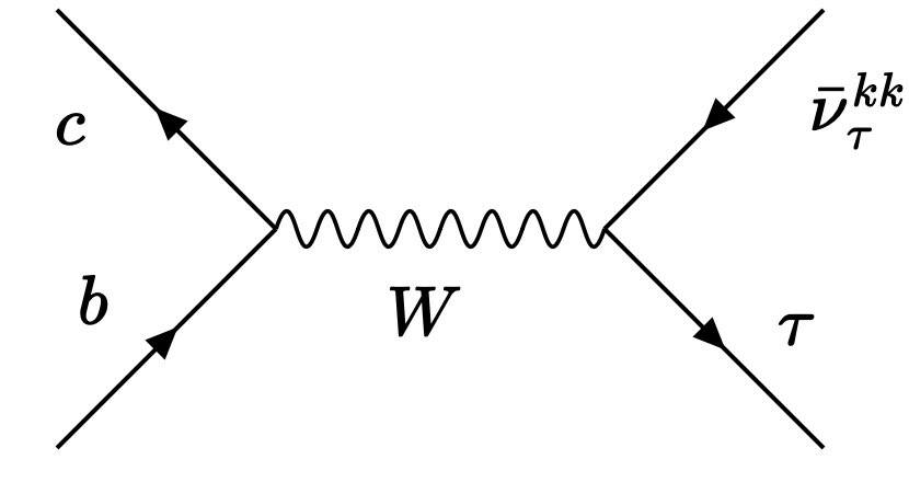
Figure 1: The relevant Feynman diagram of $b\rightarrow c\tau\bar{\nu}_{\tau}^{KK}$ transition that contributes to the same experimental signatures of $B\to D^{(*)}\tau\bar{\nu}$ decay.

Therefore, together with the new contributions from the KK neutrinos, the prediction for $R_{D^{(*)}}$ is

$$R_{D^{(*)}} =\dfrac{Br(B\rightarrow D^{(*)}\tau\bar{\nu}_{\tau})+Br(B\rightarrow D^{(*)}\tau\bar{\nu}_{\tau}^{KK})}{[(Br(B\rightarrow D^{(*)}e\bar{\nu}_{e}+Br(B\rightarrow D^{(*)}\mu\bar{\nu}_{\mu}))/2]}\approx R_{D^{(*)}}^{SM}\left(1+\frac{\Gamma(B\rightarrow D^{(*)}\tau\bar{\nu}_{\tau}^{KK}))}{\Gamma^{SM}(B\rightarrow D^{(*)}\tau\bar{\nu}_{\tau}))}\right)$$ (22)

$$\approx R_{D^{(*)}}^{SM}\left(1+\ \sum_{n=1}^{+\infty}\eta_{n}B_{\tau,n}^{*}B_{\tau,n}\right)=R_{D^{(*)}}^{SM}\left(1+\dfrac{h_{\tau}^{2}v^{2}M_{P}^{\frac{4}{\delta}-2}}{M_{F}^{\frac{4}{\delta}}}S_{\delta}R^{\delta-2}\int_{\frac{1}{R}}^{m_{B}-m_{D^{(*)}}-m_{\tau}}\frac{E^{\delta-1}}{m^{2}+E^{2}}\eta(E)dE\right),$$

where $m^{2}=\dfrac{h_{\tau}^{2}v^{2}M_{F}^{2}}{2M_{P}^{2}}$ and $\eta_{n}$ are the effects from three-body phase, having $\eta(E)$ as the corresponding transformation of $\eta_{n}$ (see the Appendix for the details) after summing up over all the contributions from KK neutrinos while invoking Eq. (20). Also note that we have $\dfrac{1}{R}\simeq\dfrac{M_{F}^{\frac{2}{\delta}+1}}{M_{P}^{\frac{2}{\delta}}}$ from the fundamental relation between $M_{P}$ and $M_{F}$. To fit the $R_{D}$ central value, the needed $M_{F}$ is about $7~{}{\rm TeV}$ for Yukawa coupling $h_{\tau}=1$, which is excluded by the LHC mono-jet plus missing energy search ATLAS:2021kxv that imposes a lower bound $M_{F}\gtrsim 11.2~{}{\rm TeV}$. Therefore, we choose Yukawa coupling $h_{\tau}=5$ for our benchmark value throughout this paper unless otherwise stated. Fig. 2 shows the relation between fundamental scale $M_{F}$ and $R_{D^{(*)}}$.

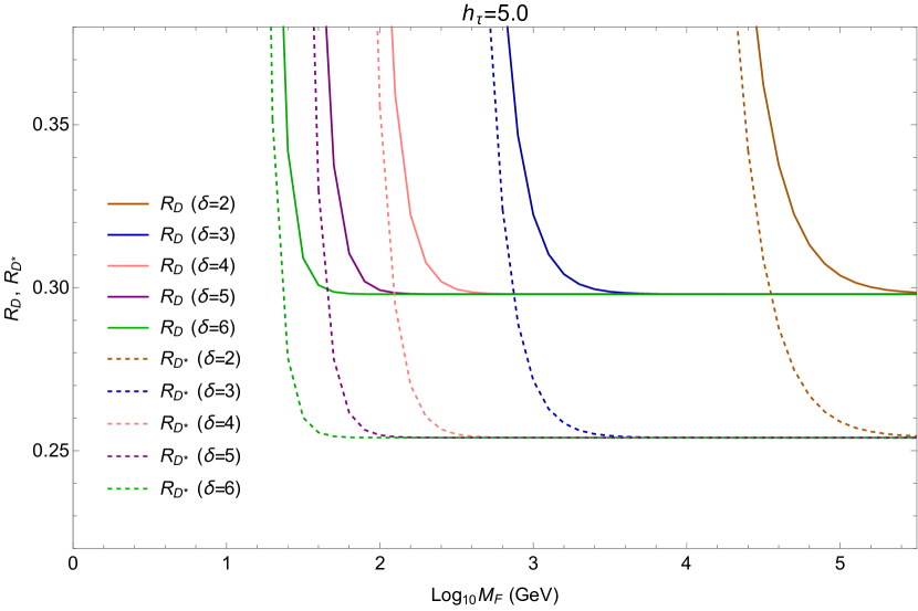
Figure 2: The plot of $M_{F}$ vs $R_{D^{(*)}}$ for a fixed Yukawa coupling strength $h_{\tau}=5$. The solid lines represent the $R_{D}$ while the dashed lines represent the $R_{D^{*}}$.

The plots are made by plugging in the SM central values of $R_{D^{(*)}}^{SM}$ HFLAV:2022pwe in eq. (41). The solid and dashed lines represent the $R_{D}$ and $R_{D^{*}}$, respectively, for $\delta=2,3,4,5,$ and 6. Clearly as fundamental scale $M_{F}$ increases, $R_{D^{(*)}}$ approach to the SM values. The best fit of the most recent experimental central values of $R_{D^{(*)}}^{exp}$ HFLAV:2023prelim with Yukawa coupling $h_{\tau}=5$ are

$$M_{F}=33\>\textrm{TeV},\>748\>\textrm{GeV},\>127\>\textrm{GeV},\>46\>\textrm{GeV},\>24\>\textrm{GeV}\>\>\>\>\>\textrm{for}\>\>R_{D}\,,$$ (23)

$$M_{F}=42\>\textrm{TeV},\>834\>\textrm{GeV},\>135\>\textrm{GeV},\>48\>\textrm{GeV},\>24\>\textrm{GeV}\>\>\>\>\>\textrm{for}\>\>R_{D^{*}}\,,$$ (24)

corresponding to $\delta=2,3,4,5,6$. It is clear that the fundamental scales $M_{F}$ are excluded by LHC searches, even when $h_{\tau}$ is increased up to $4\pi$, except for $\delta=2$. Hence, the only feasible scenario is when $\delta=2$.

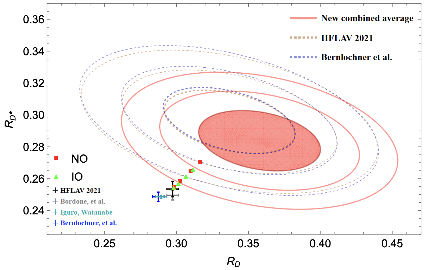
Figure 3: The upper panel shows the ($1\sigma,2\sigma,3\sigma$) contour plots of the experimental results of $R_{D}$ and $R_{D^{*}}$ of the world average (red) Iguro in mid-autumn 2022, HFLAVCollaboration HFLAV 2021 average results (dashed orange) and with Bernlochner (dashed purple). The Standard Model (SM) predictions are denoted by the crosses UBernlochner ; Watanabe ; Bordonea ; Bordoneb . The pairs of points $(R_{D},R_{D^{*}})$ in normal (inverted) ordering are shown in red squares (green triangles) with Yukawa couplings $h_{\tau}=1,5,8,10$ and fixed $M_{F}=110(128)$ TeV. The lower panel shows the most updated results of the combined new world average using the most recent results of LHCb HFLAV:2023prelim , and the global picture is almost the same as in upper panel.

The Fig. 3 shows the ($1\sigma,2\sigma,3\sigma$) contour plots between $R_{D}$ and $R_{D^{*}}$ taken from Iguro ; HFLAVCollaboration ; Bernlochner . The Standard Model predictions are the crosses UBernlochner ; Watanabe ; Bordonea ; Bordoneb . Along with the $KK$ neutrinos contributions to $R_{D}$ and $R_{D^{*}}$ the four pairs of points ($R_{D},R_{D^{*}}$) are plotted corresponding to Yukawa couplings $h_{\tau}=1,5,8,10$ with fixed $M_{F}=110$ TeV and $M_{F}=128$ TeV derived from the lower bounds Forero:2022skg in neutrino fittings for normal and inverted ordering, respectively. It can be observed that as Yukawa coupling increases the contributions from KK neutrinos increase, and as a result, predictions of $R_{D^{(*)}}$ are more close to the experimental central values of the new world average Iguro .

In the case of normal ordering the two points corresponding to $h_{\tau}=5$ and $h_{\tau}=8$ lie within the $3\sigma$ of the world average, while the point with $h_{\tau}=1$ lies outside $3\sigma$, and lastly the point with $h_{\tau}=10$ lies within $2\sigma$. Moreover, in inverted ordering the points with $h_{\tau}=8$ and $h_{\tau}=10$ lie within $3\sigma$, and the remaining two points lie outside $3\sigma$. With regards to the most updated results from LHCb shown in lower panel, the global picture of the combined world average will not change.

IV Constraints from $\tau$ decays

Now let’s consider constraints for the predictions of $R_{D}$ and $R_{D^{*}}$. Since the new contributions come from the $\tau$ lepton sector only, the most relevant and stringent constraints we consider are the experimental bounds for rare $\tau$ decays, including $\tau\rightarrow e\gamma$, $\tau\rightarrow\mu\gamma$, $\tau\rightarrow e\mu^{+}\mu^{-}$ and $\tau\rightarrow\mu e^{+}e^{-}$.

After summing up all the KK neutrino modes, the expression of the branching ratios of $\tau\rightarrow l^{{}^{\prime}}\gamma$ is given as Ioannisian:1999cw

$$Br(l\rightarrow l^{{}^{\prime}}\gamma)\approx\frac{\alpha^{3}_{w}\,s^{2}_{w}}{1024\pi^{2}}\,\frac{m^{4}_{\tau}}{M^{4}_{W}}\,\frac{m_{\tau}}{\Gamma_{\tau}}\,(s^{\nu_{\tau}}_{L})^{2}\,(s^{\nu_{l^{{}^{\prime}}}}_{L})^{2}\,,$$ (25)

where $M_{W}$ is the mass of $W$-boson, $\alpha_{w}=\frac{g_{w}^{2}}{4\pi}$ with $g_{w}$ being the $SU(2)_{L}$ coupling strength, $s_{w}=\sin\theta_{w}$ with $\theta_{w}$ being the weak mixing angle, and $\ell^{\prime}=e,~{}\mu$. The current experimental value from, $Br_{\text{exp}}(\tau\rightarrow e\gamma)<3.3\times 10^{-8}$ and $Br_{\text{exp}}(\tau\rightarrow\mu\gamma)<4.2\times 10^{-8}$ Workman:2022ynf at 90$\%$ confidence level (CL), and $\Gamma_{\tau}=2.23\times 10^{-12}$ GeV using the mean-lifetime of $\tau$ lepton in Workman:2022ynf , one obtains the lower limits

$$M_{F}>\begin{cases}67\>\textrm{TeV}&\textrm{for}\>\>\>\tau\rightarrow e\gamma\,,\\ 63\>\textrm{TeV}&\textrm{for}\>\>\>\tau\rightarrow\mu\gamma\,,\end{cases}$$ (26)

by setting $h_{e}=h_{\mu}=1$ and $h_{\tau}=5$. The next constraints come from the three-body decay of $\tau$ lepton, namely $\tau\rightarrow e\mu\mu$ and $\tau\rightarrow\mu ee$. The corrresponding branching ratios are given by Ioannisian:1999cw

$$Br(\tau\rightarrow e\mu\mu) =\dfrac{\alpha_{w}^{4}}{98304}\dfrac{m_{\tau}^{4}}{M_{W}^{4}}\dfrac{M_{F}^{4}}{M_{W}^{4}}d_{\delta}^{2}(s_{L}^{\nu_{\tau}})^{2}(s_{L}^{\nu_{e}})^{2}\Bigg{\{}(s_{L}^{\nu_{\mu}})^{4}+2(1-2s_{w}^{2})(s_{L}^{\nu_{\mu}})^{4}\big{[}\sum_{l=e,\mu,\tau}{(s_{L}^{\nu_{l}})^{2}}\big{]}$$

$$+8s_{w}^{4}\big{[}\sum_{l=e,\mu,\tau}(s_{L}^{\nu_{l}})^{2}\big{]}^{2}\Bigg{\}}\,,$$ (27)

$$Br(\tau\rightarrow\mu ee) =\dfrac{\alpha_{w}^{4}}{98304}\dfrac{m_{\tau}^{4}}{M_{W}^{4}}\dfrac{M_{F}^{4}}{M_{W}^{4}}d_{\delta}^{2}(s_{L}^{\nu_{\tau}})^{2}(s_{L}^{\nu_{\mu}})^{2}\Bigg{\{}(s_{L}^{\nu_{e}})^{4}+2(1-2s_{w}^{2})(s_{L}^{\nu_{e}})^{4}\big{[}\sum_{l=e,\mu,\tau}{(s_{L}^{\nu_{l}})^{2}}\big{]}$$

$$+8s_{w}^{4}\big{[}\sum_{l=e,\mu,\tau}(s_{L}^{\nu_{l}})^{2}\big{]}^{2}\Bigg{\}}\,,$$ (28)

where $d_{\delta}=d_{2}=\frac{\pi^{2}}{12\ln^{2}(M_{P}/M_{F})}\lesssim 1$ is a dimension-dependent factor. The current experimental bounds $Br(\tau\rightarrow e\mu\mu)<2.7\times 10^{-8}$ and $Br(\tau\rightarrow\mu ee)<1.8\times 10^{-8}$ Workman:2022ynf give

$$M_{F}>\begin{cases}54\>\textrm{TeV}&\textrm{for}\>\>\>\tau\rightarrow e\mu\mu\,,\\ 60\>\textrm{TeV}&\textrm{for}\>\>\>\tau\rightarrow\mu ee\,,\end{cases}$$ (29)

with $h_{\tau}=5$ and $h_{e}=h_{\mu}=1$. The last constraints are from the fittings of various neutrino experiments. It is shown that the upper bounds on the size of the extra dimension should be smaller than $0.2~{}{\rm\mu m}$ and $0.1~{}{\rm\mu m}$ at $90~{}\%$ C.L. for normal and inverted ordering, respectively Forero:2022skg .

The corresponding lower limits of fundamental scale for $\delta=2$ are given as

$$M_{F}>110\>(128)\>\textrm{TeV}\,,$$ (30)

for normal ordering (inverted ordering).

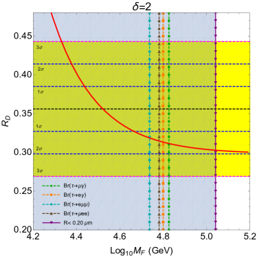
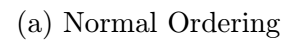
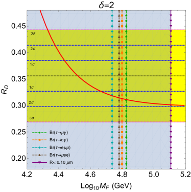
Figure 4: The left (right) panel of Fig. 4(a) and Fig. 4(b) is the plot of $M_{F}$ vs $R_{D^{(*)}}$ for $\delta=2$ with Yukawa coupling $h_{\tau}=5$ together with the following constraints: (i.) Br$(\tau\rightarrow e\mu\mu)<2.7\times 10^{-8}$ (dashed cyan), (ii.) Br$(\tau\rightarrow\mu ee)<1.8\times 10^{-8}$ (dashed brown) , (iii.) Br$(\tau\rightarrow\mu\gamma)<4.2\times 10^{-8}$ (dashed green), (iv.) Br$(\tau\rightarrow e\gamma)<3.3\times 10^{-8}$ (dashed orange) Workman:2022ynf , and (v.) neutrino bounds (solid purple) Forero:2022skg . The yellow bands give $1\sigma$, $2\sigma$ and $3\sigma$ regions of $R_{D^{(*)}}^{exp}$. The dashed black lines determine the central values of $R_{D^{(*)}}^{exp}$, while dashed blue and red lines are the boundaries of $1\sigma$ and $2\sigma$ , and $3\sigma$ regions of $R_{D^{(*)}}^{exp}$. The data we used here is the most updated world average HFLAV:2023prelim .

Fig. 4 summarises the data of $R_{D^{(*)}}$ for $\delta=2$ with Yukawa coupling $h_{\tau}=5$ together with the experimental bounds on $M_{F}$ from $Br(\tau\rightarrow e\mu\mu)$, $Br(\tau\rightarrow\mu ee)$, $Br(\tau\rightarrow\mu\gamma)$, $Br(\tau\rightarrow e\gamma)$ and neutrino oscillations. The yellow bands determine the $1\sigma$, $2\sigma$ and $3\sigma$ regions of $R_{D^{(*)}}$. The horizontal dashed lines give the central values, and boundaries of $1\sigma$, $2\sigma$ and $3\sigma$ of $R_{D^{(*)}}^{exp}$. The most stringent bound comes from the size of extra dimensions for normal and inverted ordering in Forero:2022skg . As determined in (30), these lower limits correspond to $R_{D}=0.304\>(0.301)$ and $R_{D^{*}}=0.259\>(0.257)$, for normal (inverted) ordering, respectively. All these $R_{D^{(*)}}$ predictions can be found very near to the boundary of $2\sigma$ below from the central values of $R_{D^{(*)}}^{exp}$ for both NO and IO, respectively.

V Conclusion

A possible violation of the lepton flavor universality can be found in anomalies involving rare B meson decays. This is a positive sign of physics beyond the SM. A newly calculated world average of the data by different experimental groups BaBar, Belle, and LHCb collaboration strongly supports again the leptonic flavor universality violation in the $b\rightarrow c\tau\bar{\nu}_{\tau}$ transition. We show in this work that it is possible to explain these anomalies in the extra-dimensional framework, where the Planck scale $M_{P}$ is lowered to the fundamental scale $M_{F}$. By introducing three right-handed neutrinos propagating in the bulk, the contributions from their corresponding KK neutrino modes after compactification give a plausible description of the anomalies through mixings from the active neutrinos. The central values $R_{D}^{exp}=0.356$ and $R_{D^{*}}^{exp}=0.284$ ruled out the cases $\delta=3,4,5,$ and 6 since the needed values of $M_{F}$ are lower than the bounds from LHC searches. As a result, we only considered the very special number of extra dimensions $\delta=2$. The most severe bounds from neutrino experiments on the size of large extra dimension are $R<0.2\mu m$ and $R<0.1\mu m$ for NO and IO, respectively. To satisfy these bounds the lower limits for the fundamental scale $M_{F}$ must be 110 TeV and 128 TeV, for NO and IO, respectively. With Yukawa coupling strength $h_{\tau}=5$, the predictions for $R_{D}$ and $R_{D^{*}}$ with the corresponding lower limits of $M_{F}$ from neutrino experiments are 0.304 (0.301) and 0.259 (0.257) on the boundary of $2\sigma$ contour, respectively, for NO (IO). Apparently, there is a tension between central values of $R_{D^{(*)}}^{exp}$ with the lower bounds from neutrino experiments. The future measurements of $R_{D^{(*)}}^{exp}$ will exclude this extra dimensional model with right-handed neutrino propagating in the bulk, if the central values stay.

Appendix

The three-body phase of $B\to D\tau\nu_{\tau}^{(n)KK}$ is given as

$$\int_{y^{(n)}_{min}}^{y_{max}}\int_{x^{(n)}_{min}}^{x^{(n)}_{max}}(x+y+s)(t^{(n)}-x-y)dxdy\,,$$ (31)

where

$$s=-(m_{D^{(*)}}^{2}+m_{\tau}^{2}),\>\>\>\>\ t^{(n)}=(m_{B}^{2}+m_{KK}^{(n)2})\,.$$ (32)

. The lower and upper limits in variable $y$ are

$$y_{min}^{(n)}=(m^{(n)}_{KK}+m_{\tau})^{2},\>\>\>\>\ y_{max}=(m_{B}-m_{D^{(*)}})^{2}\,,$$ (33)

while the lower and upper limits for variable $x$ can be written in terms of $y$

$$x^{(n)}_{max/min}=\dfrac{-(y^{2}+A^{(n)}-yB^{(n)})\pm\sqrt{(y^{2}+A^{(n)}-yB^{(n)})^{2}-4y(yC^{(n)}+D^{(n)})}}{2y}\,,$$ (34)

such that the expressions for $A^{(n)},B^{(n)},C^{(n)}$, and $D^{(n)}$ are the following:

$$A^{(n)} =(m_{\tau}^{2}-m_{KK}^{(n)2})(m_{B}^{2}-m_{D^{(*)}}^{2})\,,$$ (35)

$$B^{(n)} =(m_{B}^{2}+m_{D^{(*)}}^{2}+m_{KK}^{(n)2}+m_{\tau}^{2})\,,$$ (36)

$$C^{(n)} =(m_{D^{(*)}}^{2}-m_{KK}^{(n)2})(m_{B}^{2}-m_{\tau}^{2})\,,$$ (37)

$$D^{(n)} =(m_{KK}^{(n)2}m_{B}^{2}-m_{D^{(*)}}^{2}m_{\tau}^{2})(m_{B}^{2}-m_{D^{(*)}}^{2}+m_{KK}^{(n)2}-m_{\tau}^{2}).$$ (38)

Here $m_{B}$, $m_{D^{(*)}}$, $m^{(n)}_{KK}$, and $m_{\tau}$ are the masses of the B-meson, D-meson, KK mass eigenstates, and tau lepton respectively. When we sum over $n$, the integration replacement of the discrete sum in Eq. (20) transforms Eq. (31) into

$$S_{\delta}R^{\delta-2}\int_{\frac{1}{R}}^{m_{B}-m_{D^{(*)}}-m_{\tau}}\frac{E^{\delta-1}}{m^{2}+E^{2}}\times\int_{y_{min}}^{y_{max}}\int_{x_{min}}^{x_{max}}(x+y+s)(t-x-y)dxdydE\,,$$ (39)

such that $m^{2}=\dfrac{h_{\tau}^{2}v^{2}M_{F}^{2}}{2M_{P}^{2}}$ and every appearance of $m^{(n)}_{KK}$ in the expression

$$\int_{y^{(n)}_{min}}^{y_{max}}\int_{x^{(n)}_{min}}^{x^{(n)}_{max}}(x+y+s)(t^{(n)}-x-y)dxdy\,,$$ (40)

is replaced by variable $E$. The prediction for $R_{D^{(*)}}$ with contributions from the KK neutrinos is given by

$$R_{D^{(*)}} =\dfrac{Br(B\rightarrow D^{(*)}\tau\bar{\nu}_{\tau})+Br(B\rightarrow D^{(*)}\tau\bar{\nu}_{\tau}^{KK})}{[(Br(B\rightarrow D^{(*)}e\bar{\nu}_{e}+Br(B\rightarrow D^{(*)}\mu\bar{\nu}_{\mu}))/2]}\approx R_{D^{(*)}}^{SM}\left(1+\frac{\Gamma(B\rightarrow D^{(*)}\tau\bar{\nu}_{\tau}^{KK}))}{\Gamma^{SM}(B\rightarrow D^{(*)}\tau\bar{\nu}_{\tau}))}\right)$$ (41)

$$\approx R_{D^{(*)}}^{SM}\left(1+\ \sum_{n=1}^{+\infty}\eta_{n}B_{\tau,n}^{*}B_{\tau,n}\right)=R_{D^{(*)}}^{SM}\left(1+\dfrac{h_{\tau}^{2}v^{2}M_{P}^{\frac{4}{\delta}-2}}{M_{F}^{\frac{4}{\delta}}}S_{\delta}R^{\delta-2}\int_{\frac{1}{R}}^{m_{B}-m_{D^{(*)}}-m_{\tau}}\frac{E^{\delta-1}}{m^{2}+E^{2}}\eta(E)dE\right),$$

where

$$\eta_{n}=\dfrac{\int_{y^{(n)}_{min}}^{y_{max}}\int_{x^{(n)}_{min}}^{x^{(n)}_{max}}(x+y+s)(t^{(n)}-x-y)dxdy}{\int_{y_{min}}^{y_{max}}\int_{x_{min}}^{x_{max}}(x+y+s)(t-x-y)dxdy\>\>\Big{|}_{SM}},~{}~{}\eta(E)=\eta_{n}\>\>\Big{|}_{m^{(n)}_{KK}=E}\,.$$ (42)

References

(1)
[LHCb],
[arXiv:2212.09152 [hep-ex]].
(2)
Y. Amhis et al. [HFLAV],
[arXiv:2206.07501 [hep-ex]].
(3)
S. Iguro, T. Kitahara and R. Watanabe, doi:10.48550/arXiv.2210.10751
[arXiv:2210.10751 [hep-ph]]
(4)
https://indico.cern.ch/event/1231797/
(5)
G. Hiller, D. Loose and I. Nišandžić,
JHEP 06, 080 (2021);
B. Gripaios, M. Nardecchia and S. A. Renner,
JHEP 05, 006 (2015);
R. Barbieri, C. W. Murphy and F. Senia,
Eur. Phys. J. C 77, no.1, 8 (2017);
B. Fornal, S. A. Gadam and B. Grinstein,
Phys. Rev. D 99, no.5, 055025 (2019);
C. Cornella, J. Fuentes-Martin and G. Isidori,
JHEP 07, 168 (2019);
O. Popov, M. A. Schmidt and G. White,
Phys. Rev. D 100, no.3, 035028 (2019);
I. Bigaran, J. Gargalionis and R. R. Volkas,
JHEP 10, 106 (2019);
C. Hati, J. Kriewald, J. Orloff and A. M. Teixeira,
JHEP 12, 006 (2019);
A. Datta, J. L. Feng, S. Kamali and J. Kumar,
Phys. Rev. D 101, no.3, 035010 (2020);
P. S. Bhupal Dev, R. Mohanta, S. Patra and S. Sahoo,
Phys. Rev. D 102, no.9, 095012 (2020);
M. Du, J. Liang, Z. Liu and V. Q. Tran,
K. Ban, Y. Jho, Y. Kwon, S. C. Park, S. Park and P. Y. Tseng,
(6)
E. Megias, M. Quiros and L. Salas,
JHEP 07, 102 (2017);
X. G. He and G. Valencia,
Phys. Lett. B 779, 52-57 (2018);
S. Matsuzaki, K. Nishiwaki and R. Watanabe,
JHEP 08, 145 (2017);
K. S. Babu, B. Dutta and R. N. Mohapatra,
JHEP 01, 168 (2019);
A. Greljo, D. J. Robinson, B. Shakya and J. Zupan,
JHEP 09, 169 (2018);
P. Asadi, M. R. Buckley and D. Shih,
JHEP 09, 010 (2018)
(7)
M. Tanaka,
Z. Phys. C 67, 321-326 (1995);
A. Celis, M. Jung, X. Q. Li and A. Pich,
JHEP 01, 054 (2013);
A. Celis, M. Jung, X. Q. Li and A. Pich,
Phys. Lett. B 771, 168-179 (2017);
S. Iguro and K. Tobe,
Nucl. Phys. B 925, 560-606 (2017);
S. Fraser, C. Marzo, L. Marzola, M. Raidal and C. Spethmann,
Phys. Rev. D 98, no.3, 035016 (2018);
R. Martinez, C. F. Sierra and G. Valencia,
Phys. Rev. D 98, no.11, 115012 (2018);
(8)
R. Barbieri, P. Creminelli and A. Strumia
Nucl. Phys. B 585, 28-44 (2000)
doi:10.1016/S0550-3213(00)00348-5
[arXiv:hep-ph/0002199 [hep-ph]]
(9)
D. V. Forero, C. Giunti, C. A. Ternes and O. Tyagi,
Phys. Rev. D 106, no.3, 035027 (2022)
doi:10.1103/PhysRevD.106.035027
[arXiv:2207.02790 [hep-ph]].
(10)
N. Arkani-Hamed, S. Dimopoulos, G. Dvali and J. March-Russell,
Phys. Rev. D 65, 024032 (2001)
doi:10.1103/PhysRevD.65.024032
[arXiv:hep-ph/9811448 [hep-ph]].
(11)
K.R. Dienes, E. Dudas and T. Gherghetta,
Nucl. Phys. B 557, 25 (1999)
doi:10.1016/S0550-3213(99)00377-6
[arXiv:hep-ph/9811428 [hep-ph]].
(12)
G. R. Dvali and A. Y. Smirnov, Nucl. Phys. B 563, 63 (1999)
doi:10.1016/S0550-3213(99)00574-X
[arXiv:hep-ph/9904211 [hep-ph]]
(13)
A. Ioannisian and A. Pilaftsis,
Phys. Rev. D 62, 066001 (2000)
doi:10.1103/PhysRevD.62.066001
[arXiv:hep-ph/9907522 [hep-ph]].
(14)
R. N. Mohapatra and A. Perez-Lorenzana, Nucl. Phys. B 593, 451 (2001)
doi:10.1016/S0550-3213(00)00634-9
[arXiv:hep-ph/0006278 [hep-ph]]
(15)
P. Langacker, D. London, Phys. Rev. D 38, 886 (1988)
doi:org/10.1103/PhysRevD.38.886.
(16)
J.C. Aban, C.R. Chen and C.S. Nugroho, Phys. Lett. B 830, 137164 (2022)
doi:10.1016/j.physletb.2022.137164
[arXiv:hep-ph/2112.12477 [hep-ph]]
(17)
J. Schechter and J.W.F. Valle, Phys. Rev. D 22, 2227 (1980)
doi:10.1103/PhysRevD.22.2227.
(18)
G. Aad et al. [ATLAS],
Phys. Rev. D 103, no.11, 112006 (2021)
doi:10.1103/PhysRevD.103.112006
[arXiv:2102.10874 [hep-ex]].
(20)
F. U. Bernlochner, M. F. Sevilla, D. J. Robinson, and G. Wormser, Rev. Mod. Phys. 94, 015003 (2022)
[arXiv:2101.08326] [hep-ex]]
(21)
F. U. Bernlochner, M. F. Sevilla, D. J. Robinson and G. Wormser,
Rev. Mod. Phys. 94, no.1, 015003 (2022)
doi:10.1103/RevModPhys.94.015003
[arXiv:2101.08326 [hep-ex]].
(22)
S. Iguro and R. Watanabe,
JHEP 08, no.08, 006 (2020)
doi:10.1007/JHEP08(2020)006
[arXiv:2004.10208 [hep-ph]].
(23)
M. Bordone, M. Jung and D. van Dyk,
Eur. Phys. J. C 80, no.2, 74 (2020)
doi:10.1140/epjc/s10052-020-7616-4
[arXiv:1908.09398 [hep-ph]].
(24)
M. Bordone, N. Gubernari, D. van Dyk and M. Jung,
Eur. Phys. J. C 80, no.4, 347 (2020)
doi:10.1140/epjc/s10052-020-7850-9
[arXiv:1912.09335 [hep-ph]].
(25)
R. L. Workman et al. [Particle Data Group],
PTEP 2022, 083C01 (2022)
doi:10.1093/ptep/ptac097