Existence of minimizers for the SDRI model in $\mathbb{R}^{n}$: Wetting and dewetting regimes with mismatch strain

Abstract.

The existence and the regularity results obtained in [37] for the variational model introduced in [36] to study the optimal shape of crystalline materials in the setting of stress-driven rearrangement instabilities (SDRI) are extended from two dimensions to any dimensions $n\geq 2$. The energy is the sum of the elastic and the surface energy contributions, which cannot be decoupled, and depend on configurational pairs consisting of a set and a function that model the region occupied by the crystal and the bulk displacement field, respectively. By following the physical literature, the “driving stress” due to the mismatch between the ideal free-standing equilibrium lattice of the crystal with respect to adjacent materials is included in the model by considering a discontinuous mismatch strain in the elastic energy. Since two-dimensional methods and the methods used in the previous literature where Dirichlet boundary conditions instead of the mismatch strain and only the wetting regime were considered, cannot be employed in this setting, we proceed differently, by including in the analysis the dewetting regime and carefully analyzing the fine properties of energy-equibounded sequences. This analysis allows to establish both a compactness property in the family of admissible configurations and the lower-semicontinuity of the energy with respect to the topology induced by the $L^{1}$-convergence of sets and a.e. convergence of displacement fields, so that the direct method can be applied. We also prove that our arguments work as well in the setting with Dirichlet boundary conditions.

1. Introduction

Elastic effects can strongly affect the structure of crystalline materials by inducing morphological destabilizations from the optimal free-standing crystalline equilibrium, that are often referred to as the family of stress-driven rearrangement instabilities (SDRI) [4, 19, 30, 34, 48]. In order to relieve the strain, atoms move from their crystalline order possibly inducing both bulk deformations and interface irregularities. The latter can be originated in various forms, such as the roughness of the exposed crystalline boundaries, the formation of internal cracks in the bulk, the nucleation of dislocations in the crystalline lattice, and the delamination at contact edges with adjacent materials. However, such corrugations and extra boundary interfaces are not favorable with respect to the surface energy, which would instead prescribe regular specific Wulff/Winterbottom-type shapes [44, 45, 50, 51]. Therefore, the surface energy competes against the destabilizing effect of the elastic energy with a regularizing effect: a delicate microscopical compromise between such opposite mechanisms must then be reached strongly affecting in a variety of ways the original crystalline-material macroscopical properties.

In the strive of capturing such interplay between elastic and (anisotropic) surface energy described by the physical literature [25, 35, 39, 46, 47, 49, 52], various mathematical models with a variational nature have been introduced in relation to the different settings relevant for the applications. A non-exhaustive list includes [6, 9, 20, 21, 27, 33, 38] for epitaxially-strained thin films deposited on supporting materials, [10, 11, 29] for fractures, [5, 40] for delamination, and, e.g., [28] for crystalline cavities. Establishing the existence of minimizers for such models even in dimension $n=2$ is a challenging task especially due to compactness issues. Such issues were first solved in simplified settings, by working under the antiplane-shear assumption [8, 16], or by distinguishing the applications with adhoc geometric assumptions on the morphology of the crystalline materials, such as adopting graph-type and star-shapedness constraints on film profiles and crystal cavities, respectively. More recently, the development of several techniques related to GSBD-functions, a specific subclass of functions of bounded deformation [18], have been sucessfully applied to models related to the Griffith energy [11, 12, 13, 14, 18, 29]. Following this progress, there has been a growing effort [15, 17, 36, 37] to develop mathematical frameworks enabling the simultaneous treatment of the various mechanisms of mass rearrangement and boundary instabilities, which is of crucial importance, as often such phenomena concomitantly occur in applications.

The aim of this paper is to extend to dimension $n\geq 2$, and hence including the physical relevant case of $n=3$, the existence and the regularity results obtained in [37] for $n=2$ for the SDRI model introduced in [36]. In regard of the existence, such an extension was previously achieved in [17] for the wetting regime, i.e., the case for which it is more convenient for the crystal material to always cover the surface of a (supporting) adjacent material rather than letting it exposed, and the setting in which the stress driving effect characterizing SDRI is mathematically prescribed by introducing boundary Dirichlet conditions. Here we address also the dewetting regime and, as previously done by the authors in [36, 37] for $n=2$, by following the physical literature [4, 19, 30, 34, 47, 48, 52] we avoid the use of any Dirichlet boundary conditions and we directly introduce a mismatch strain in the elastic energy. As suggested by its name, such strain is induced in the free crystal, i.e., the crystal of which we are studying the morphology, by the mismatch between its ideal free-standing equilibrium lattice and the lattice of adjacent materials. Since the approach used in [17] cannot be applied to this setting without boundary conditions as it is described below (see also [37]), we have developed an alternative strategy that allows us to tackle both the case with mismatch strain and the one with Dirichlet conditions (see Remark 2.10 for more details). Finally, the method of this paper extends (also to both the settings with and without Dirichlet conditions) the regularity results for the bulk displacements and the morphologies of the energy minimizing configurations obtained by the authors in [37] for $n=2$ (besides extending the existence results of [37] to the presence of different adjacent materials and to Griffith-type models with mismatch strain and delamination).

To facilitate this generalization, we adopt the terminology introduced in [36, 37], by referring to the bounded region $\Omega$ in the space $\mathbb{R}^{n}$ where the free crystal is located as the container in analogy to capillarity problems, and to the region $S$ occupied by adjacent materials outside the container, i.e., $S\subset\mathbb{R}^{n}\setminus\Omega$, as the substrate in analogy to the thin-film setting where $S$ is the supporting material on which the film is being deposited. We notice that the contact region between the container and the substrate $\Sigma:=\partial\Omega\cap\partial S$ is assumed to be a Lipschitz $(n-1)$-manifold and that $S$ can be given by a finite number of different connected components possibly modeling different adjacent materials. The free crystals are then represented by configurational pairs of set-function type $(A,u)$, where $A\subset\Omega$ is a set of finite perimeter denoting the region occupied by the free crystal and subject to the volume constraint $|A|=\mathtt{v}$ with $\mathtt{v}\in(0,|\Omega|]$, and $u$ is a vector valued faction in $GSBD^{2}(\rm{Int}(A\cup\Sigma\cup S))\color[rgb]{0,0,0}\cap H_{\mathrm{loc}}^{1}(S)\color[rgb]{0,0,0}$ denoting the displacement field of the free-crystal and substrate bulk materials with respect to their optimal equilibrium arrangements. The family of all such admissible configurational pairs $(A,u)$ is denoted by $\mathcal{C}$.

The configurational energy of any free-crystal pair $(A,u)\in\mathcal{C}$ is defined by

$$\mathcal{F}(A,u)=\mathcal{W}(A,u)+\mathcal{S}(A,u),$$ (1.1)

where $\mathcal{S}$ and $\mathcal{W}$ represent the elastic and the surface energy, respectively. The elastic energy $\mathcal{W}$ in (1.1) is defined as in [27] by

$$\mathcal{W}(A,u)=\int_{A\cup S}\mathbb{C}(x)[\mathcal{E}u-\mathbf{M}_{0}]:[\mathcal{E}u-\mathbf{M}_{0}]\,\mathrm{d}x,$$

where $\mathbb{C}$ is a bounded measurable tensor-valued map $\mathbb{C}$ in $\Omega\cup S$ satisfying the coercivity assumption $\mathbb{C}\geq c\,\mathbb{I}>0$ (in the sense of linear operators), where $\mathbb{I}$ is the identity tensor, $\mathcal{E}u$ is the approximate symmetric gradient of $u$ (see (2.2)) and $\mathbf{M}_{0}$ is the (discontinuous) mismatch strain defined as

$$\mathbf{M}_{0}=\begin{cases}\mathcal{E}u_{0}&\text{in $\Omega,$}\\ 0&\text{in $S$}\end{cases}$$ (1.2)

for some fixed $u_{0}\in H^{1}(\mathbb{R}^{n})$. In the special case in which the equilibrium lattice of the free crystal and of the substrate matches at $\Sigma$, we take $u_{0}\equiv 0$. The surface energy $\mathcal{S}$ in (1.1) is defined as

$$\mathcal{S}(A,u):=\int_{\partial^{*}A\cup J_{u}}\psi(x,\nu(x))\mathrm{d}\mathcal{H}^{n-1},$$

where $\partial^{*}A$ is the reduced boundary of $A$, $J_{u}$ is the jump set of $u$, and the surface energy density $\psi(\cdot,\nu(\cdot))$ is given by

$$\psi(x,\nu(x)):=\begin{cases}\varphi(x,\nu_{A}(x))&\text{if $x\in\Omega\cap\partial^{*}A,$}\\ 2\varphi(x,\nu_{J_{u}}(x))&\text{if $x\in A^{(1)}\cap J_{u},$}\\ \beta(x)&\text{if $x\in[\Sigma\cap\partial^{*}A]\setminus J_{u},$}\\ \varphi(x,\nu_{\Sigma}(x))&\text{if $x\in\Sigma\cap\partial^{*}A\cap J_{u}$,}\end{cases}$$ (1.3)

where $\nu_{U}(x)$ denotes the outward-pointing normal vector to $U$ at $x\in\partial^{*}U$ for any set of finte perimeter $U\subset\mathbb{R}^{n}$, $\nu_{\Sigma}:=\nu_{S}$, $\nu_{J_{u}}$ is the normal on $J_{u}$, $A^{(1)}$ is the set of points of density $1$ for $A$, $\varphi\in C(\overline{\Omega}\times\mathbb{R}^{n})$ is a a Finsler norm denoting the anisotropic surface tension of the free-crystal material, and $\beta\in L^{\infty}(\Sigma)$ represents the relative adhesion coefficient of $\Sigma$ for which we assumed, as in capillarity theory (see, e.g., [24]), that

$$|\beta(x)|\leq\varphi(x,\nu_{\Sigma})\quad\text{for \color[rgb]{0,0,0}a.e.\ \color[rgb]{0,0,0}$x\in\Sigma$.}$$ (1.4)

We notice that the weights in (1.3), which forbid to decouple the surface energy from the elastic energy making the energy $\mathcal{F}$ highly nonlocal, are consistent with the ones chosen in [17, 27, 28, 36, 37], where they were crucial to prove energy lower-semicontinuity-type properties. In particular, the anisotropy on internal cracks $A^{(1)}\cap J_{u}$ is weighted twice as much as the free boundary $\Omega\cap\partial^{*}A$ of the exposed boundary of the free crystal, because cracks can be approximated by “closing voids” as in [17, 27, 36]. The presence of the surface energy over $\Sigma\cap\partial^{*}A\cap J_{u}$ allows to consider a more general framework for thin films depositing on a substrate, in which cracks are allowed to appear not only inside the film material, but also along the surface of the substrate characterizing the delamination region, where debonding between the atoms of the two materials occurs, and as such, the corresponding surface tension in (1.3) is regarded as the same of the one on the free-crystal exposed boundary. Finally, on the complementary region to the delamination in $\Sigma\cap\partial^{*}A$ where the bulk displacement is continuous, the relative adhesion coefficient $\beta$ is considered.

We observe that in the case of total wetting case, i.e., if $\beta(x)=-\varphi(x,\nu_{\Sigma}(x))$ for a.e. $x\in\Sigma,$ we reduce to the setting of material voids considered in [17] (with the mismatch strain $\mathbf{M}_{0}$ replaced by a Dirichlet boundary condition). On the contrary, in the total dewetting case, i.e., if $\beta(x)=\varphi(x,\nu_{\Sigma}(x))$ for a.e. $x\in\Sigma,$ then one can readily check that the energy $\mathcal{F}$ is minimized by configurational pairs with displacement $u\equiv u_{0}$ in $\Omega$ and null otherwise, and so characterized by having a zero elastic energy: the model reduces to the dewetted capillarity setting, or in other words, to the anisotropic isoperimetric problem in a container. Finally, in the case with $\mathtt{v}=|\Omega|$, we reduces to the Griffith model with the inclusion of possible delamination at the substrate boundary, which generalize also for $n=2$ the setting considered by the authors in [36, 37] together with $S\neq\emptyset$.

We now present the two main results of the paper (see Section 2.2 for more detailed statements) and comment their proofs. We begin by observing that, since the values of the admissible displacement fields $u$ in the void regions $\Omega\setminus A$ do not play any role in the energy of $(A,u)$, as only a formal difference with respect to the previous presentation of the SDRI models introduced in [36, 37], for every $(A,u)\in\mathcal{C}$ we can redefine $u$ in $\Omega\setminus A$ with a properly chosen constant such that $\Omega\cap\partial^{*}A\subset J_{u}$ (see Remark 2.1), and so without changing the value of $\mathcal{F}(A,u)$. We make use of this observation in the following.

Theorem 1.1 (Existence of minimizing configurations).

The minimum problem

$$\min\limits_{(A,u)\in\mathcal{C},\,|A|=\mathtt{v}}\,\,\mathcal{F}(A,u)$$ (1.5)

admits a solution.

We refer the Reader to Theorem 2.4 for a more detailed and comprehensive statement of the existence result of Theorem 1.1.

Theorem 1.1 is established by means of the direct method of the calculus of variations with respect to a properly chosen topology $\tau_{\mathcal{C}}$ with which we equip $\mathcal{C}$, and that is characterized by the convergence:

$$(A_{k},u_{k})\overset{\tau_{\mathcal{C}}}{\longrightarrow}(A,u)\qquad\Longleftrightarrow\qquad\begin{cases}A_{k}\to A\quad\text{in $L^{1}(\mathbb{R}^{n}),$}\\ u_{k}\to u\quad\text{\color[rgb]{0,0,0}a.e.\ \color[rgb]{0,0,0}in $\Omega\cup S.$}\end{cases}$$

In order to establish the $\tau_{\mathcal{C}}$-lower semicontinuity of $\mathcal{F}$ in Theorem 2.5 we consider the positive Radon measures $\mu_{k}$ and $\mu$ in $\mathbb{R}^{n}$ associated to the localized energy versions of $\mathcal{F}(A_{k},u_{k})$ and $\mathcal{F}(A,u)$, respectively, for which it holds that

$$\liminf\limits_{k\to+\infty}\mathcal{F}(A_{k},u_{k})\geq\mathcal{F}(A,u)\qquad\Longleftrightarrow\qquad\liminf\limits_{k\to+\infty}\mu_{k}(\mathbb{R}^{n})\geq\mu(\mathbb{R}^{n}).$$ (1.6)

Then, we observe that, up to a subsequence, $\mu_{k}$ weakly* converges to some positive Radon measure $\mu_{0}$, and that $\mu$ is absolutely continuous with respect to $\mathcal{H}^{n-1}\mathop{\hbox{\vrule height=9.0pt,width=0.5pt,depth=0.0pt\vrule height=0.5pt,width=5.0pt,depth=0.0pt}}\nolimits(\partial^{*}A\cup J_{u}\cup\Sigma)+\mathcal{L}^{n}\mathop{\hbox{\vrule height=9.0pt,width=0.5pt,depth=0.0pt\vrule height=0.5pt,width=5.0pt,depth=0.0pt}}\nolimits(\Omega\cup S),$ and we establish the following estimates for the Radon-Nikodym derivatives:

$$\frac{\mathrm{d}\mu_{0}}{\mathrm{d}\mathcal{H}^{n-1}\mathop{\hbox{\vrule height=9.0pt,width=0.5pt,depth=0.0pt\vrule height=0.5pt,width=5.0pt,depth=0.0pt}}\nolimits(\partial^{*}A\cup J_{u}\cup\Sigma)}\geq\frac{\mathrm{d}\mu}{\mathrm{d}\mathcal{H}^{n-1}\mathop{\hbox{\vrule height=9.0pt,width=0.5pt,depth=0.0pt\vrule height=0.5pt,width=5.0pt,depth=0.0pt}}\nolimits(\partial^{*}A\cup J_{u}\cup\Sigma)}\quad\text{$\mathcal{H}^{n-1}$ -a.e. on $\partial^{*}A\cup J_{u}\cup\Sigma,$}$$ (1.7)

$$\frac{\mathrm{d}\mu_{0}}{\mathrm{d}\mathcal{L}^{n}\mathop{\hbox{\vrule height=9.0pt,width=0.5pt,depth=0.0pt\vrule height=0.5pt,width=5.0pt,depth=0.0pt}}\nolimits(\Omega\cup S)}\geq\frac{\mathrm{d}\mu}{\mathrm{d}\mathcal{L}^{n}\mathop{\hbox{\vrule height=9.0pt,width=0.5pt,depth=0.0pt\vrule height=0.5pt,width=5.0pt,depth=0.0pt}}\nolimits(\Omega\cup S)}\quad\text{$\mathcal{L}^{n}$-a.e. in $\Omega\cup S,$}$$ (1.8)

which imply that $\lim\mu_{k}(\mathbb{R}^{n})=\mu_{0}(\mathbb{R}^{n})\geq\mu(\mathbb{R}^{n})$ and, in view of (1.6), conclude the proof of the lower-semicontinuity. For the estimate (1.7) we need to distinguish between the estimate at the reduced boundary of $A$ and at $\Sigma\setminus J_{u}$, where we can implement techniques developed in capillarity theory [1, 24], from the estimate at the (approximate) jump points of $u$, where we employ arguments based on the slicing properties of GSBD-functions as in the Griffith model [13, 14, 15], for which though extra care is needed: unless $\mathtt{v}=|\Omega|,$ we cannot directly apply those arguments because at jump points we need to obtain different weights with respect to the ones at the reduced boundary of $A.$ Rather, we replace $J_{u_{k}}$ in small “holes” up to some error by means of Corollaries 3.3 and 3.5 in such a way that each slice intersects the boundary of those holes at least in two points (see the proof of Proposition 4.1), which in turns yields the desired estimate with weight $2$ at such jump points (see Corollary 4.2). Finally, we prove (1.8) by using the convexity of $\mathcal{W}(A,\cdot)$ and by observing that the condition $u_{k}\to u$ a.e. in $\Omega\cup S,$ together with the compactness result [14, Theorem 1.1], allows us to conclude that $\mathcal{E}u_{k}\rightharpoonup\mathcal{E}u$ in $L^{2}(\Omega\cup S)$. We recall that in [17] the authors prove the lower semicontinuity of an energy for crystalline voids via relaxation arguments. Namely, the authors start in the regular family of pair configurations given by voids with a Lipschitz boundary and Sobolev displacement fields, and then in the relaxation, the jump set appears as the void boundaries collapse, resulting in a coefficient $2$ in front of the jump energy of $\mathcal{S}$. We are here actually arguing in the reverse direction: first we start in $\mathcal{C}$ with admissible pairs allowing displacements with jump sets, and then we carefully create an at most countable family of voids around them.

The $\tau_{\mathcal{C}}$-compactness of an energy-equibounded sequence $\{(A_{k},u_{k})\}\subset\mathcal{C}$ is established in Theorem 2.6. We easily get the uniform bounds on the perimeters of $A_{k}$, the $\mathcal{H}^{n-1}$- measure of the jumps $J_{u_{k}}$, and the $L^{2}$-norm of $\mathcal{E}u_{k}$ by the assumptions on the anisotropic surface tensions and the elasticity tensor (see Remark 2.3). Thus, we can directly deduce the convergence in $L^{1}(\mathbb{R}^{n})$ up to a non-relabelled subsequence of $A_{k}$ to some set $A\subset\Omega$ of finite perimeter. However, establishing the $\mathcal{L}^{n}$ a.e.  convergence of the displacements $u_{k}$ is delicate: by [14, Theorem 1.1] there could be an exceptional set $E$ with $\mathcal{L}^{n}$ positive measure, in which $|u_{k}|\to+\infty$. The presence of such an exceptional set has been previously treated by prescribing Dirichlet boundary conditions [13, 14, 17]. For instance, in [17] the compactness issue is solved by considering in the proof an auxiliary more general class $GSBD_{\infty}^{p}$, $p>1$, of displacements (which are allowed to attain the infinite value on a subset of their domain of also $\mathcal{L}^{n}$ positive measure) and then, by using the Dirichlet condition imposed on the displacements at the boundary, the authors are able to prove that the minimizing displacements belong to the original space $GSBD^{p}.$ However, as in the setting with the mismatch strain (1.2), we cannot rely on any fixed boundary condition, one cannot even exclude the situation with $E=\Omega\cup S$ and hence, this issue unfortunately forbids the implementation of the strategy of [17] to our SDRI setting. The other option of excluding the presence of the exceptional set is based on the employment of Poincaré-Korn inequality for GSBD-functions citeCCF:2016 with small jump: the set $\Omega$ is partitioned into a Caccioppoli family $\{P_{j}\}$ of sets $P_{j}$ in which a sequence $\{a_{k}^{j}\}$ of rigid displacements are defined in such a way that $u_{k}-a_{k}^{j}$ is convergent pointwise a.e. in $P_{j}$, so that one can conclude that the sequence

$$v_{k}:=u_{k}-\sum\limits_{j}a_{k}^{j}\chi_{P_{j}}$$ (1.9)

converges to some $u\in GSBD^{p}(\Omega)$ a.e. in $\Omega$, $\mathcal{E}v_{k}\rightharpoonup\mathcal{E}u$ in $L^{p}(\Omega)$, and

$$\lim\limits_{k\to+\infty}\mathcal{H}^{n-1}(J_{u_{k}})\geq\mathcal{H}^{n-1}\Big{(}J_{u}\cup(\Omega\cap\bigcup_{j}\partial^{*}P_{j})\Big{)}$$

(see [15, Theorem 1.1]). However, also this approach seems not implementable in our SDRI setting, since the functions $v_{k}$ defined in (1.9) may admit extra jumps along the boundary of the partition phases $P_{j}$ that should be counted with different weights in our setting with different surface tensions.

In view of these issues, in order to prove compactness we use a different strategy in this paper by directly partitioning the sets $A$ and $A_{k}$ (not only $A$!) into Caccioppoli families (that need to be created by starting from the connected components of the substrate) up to a controllable error (see Figures 3 and 5). Such strategy is a reminiscence of the ideas already used by the authors in [36, Theorem 2.7], of partitioning $A_{k}$ by means of introducing extra circles closing the shrinking “necks”, which though works only for $n=2$ and under the constraint assumed in [36] on the number of boundary components for the admissible free-crystal regions. More precisely, we proceed here arguing as follows: First, by the classical Poincaré-Korn inequality we partition $S$ in a family $\{S^{i}\}_{i\geq 1}$ of sets $S^{i}$ such that for each $i\geq 1$ the set $S^{i}$ is a union of connected components of $S$ and there exists a sequence of rigid displacements $\{a_{k}^{i}\}$ such that, up to a subsequence, $u_{k}-a_{k}^{i}$ converges a.e. in $S^{i}$ and $|a_{k}^{i}-a_{k}^{j}|\to+\infty$ a.e. in $\mathbb{R}^{n}$ for every $j\neq i$. Second, by applying [14, Theorem 1.1] with $u_{k}-a_{k}^{i}$ we construct a family $\{F^{i}\}_{i\geq 0}$ of pairwise disjoint Caccioppoli subsets of $A,$ such that for $i\geq 1$ the sequence $u_{k}-a_{k}^{i}$ converges a.e. in $F^{i}\cup S^{i}$ and diverges to infinity otherwise, and $F^{0}:=A\setminus\bigcup_{i\geq 1}F^{i}$. Furthermore, since $F^{0}$ is the portion of the free crystal, so-called in the following “hanging phase” (see Figure 1), that does not “interact” with any substrate component, we can redefine the displacements in $F^{0}$ as $u_{0}$ (see (1.2)), which corresponds to providing a zero contribution to the overall elastic energy. Third, by using the $\mathcal{H}^{n-1}$-rectifiability of $\partial^{*}F^{i}$ and Propositions 4.1 and 5.2, we construct for any $\delta>0$ a union $G_{k}^{\delta}\subset\Omega$ of open sets covering $\bigcup\partial^{*}F^{i}$ up to some error of order $O(\sqrt{\delta})$ and whose perimeter and volume are controlled, and we set

$$B_{k}^{\delta}:=A_{k}\setminus G_{k}^{\delta}\quad\text{and}\quad v_{k}^{\delta}:=u_{0}\chi_{F^{0}}+\sum\limits_{i\geq 1}(u_{k}-a_{k}^{i})\chi_{S^{i}\cup(F^{i}\setminus G_{k}^{\delta})}+u_{0}\chi_{F^{0}}.$$ (1.10)

We notice that actually the definition of the $v_{k}^{\delta}$ in (1.10) is more involved (see (5.3)), as we need also to control the possible large jumps created along $\Sigma$, that though in the limit disappear (becoming wetting layer), by creating artificial small jumps in $A_{k}^{\delta}\setminus A$ and redefining $v_{k}^{\delta}$ in that set near $\Sigma$. The obtained configurations satisfy

$$\mathcal{F}(A_{k},u_{k})\geq\mathcal{F}(B_{k}^{\delta},v_{k}^{\delta})-c\sqrt{\delta}\Big{(}\mathcal{H}^{n-1}(\partial^{*}A_{k})+\mathcal{H}^{n-1}(J_{u_{k}})+\sum\limits_{h=0}^{m}P(F^{h})\Big{)}$$ (1.11)

for some constant $c>0$ (see Proposition 5.1), from which Theorem 2.6 follows by a diagonal argument.

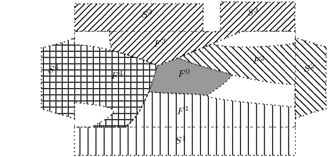
Figure 1. The partitions of the substrate and the free crystal into, respectively, the families $\{S^{i}\}_{i\geq 1}$ and $\{F^{i}\}_{i\geq 0}$ of Caccioppoli sets, which are used to prove the $\tau_{\mathcal{C}}$-compactness result, are depicted by representing the various phases of the free crystal that are interacting with the substrate with different line patterns and the remaining “hanging phase” $F^{0}$ with a point pattern.

We also notice that in the case with Dirichlet boundary conditions, one see at most 2 elements in the partition, the hanging phase $F^{0}$ and a phase $F^{1}$ interacting with the substrate, since in this case we do not need to add any rigid displacements. Apart from this simplification, the methods used in the proof of Theorems 2.5 and 2.6 still work, even by relaxing the assumptions on the convex elastic energy densities, i.e., by allowing for a $p$-growth with respect to the strains (see Section 2.3). This allows us in particular to recover in Remark 2.10 the existence results for the model representing material voids in the framework with Dirichlet boundary conditions of [17] and the existence and regularity results for the Griffith fracture model with Dirichlet boundary conditions of [13].

The second main result of the paper relates to properties of partial regularity satisfied by the minimizers $(A,u)$ of $\mathcal{F}$, such as the essential closedness of $J_{u}$ and $\partial^{*}A.$

Theorem 1.2 (Regularity results for minimizing configurations).

Let $(\widetilde{A},\widetilde{u})$ be a solution of (1.5). Then the pair $(A,u)$ defined by

$$A\color[rgb]{0,0,0}:=\color[rgb]{0,0,0}\mathrm{Int}(A^{(1)})\qquad\text{and}\qquad u\color[rgb]{0,0,0}:=\color[rgb]{0,0,0}\widetilde{u}\chi_{A\cup S}+\xi\chi_{\Omega\setminus A},$$

where $\xi\in\mathbb{R}^{n}$ is chosen such that $\Omega\cap\partial^{*}A\subset J_{u}$ (see Remark 2.1), is also a solution of (1.5). Furthermore, we have that

$$\mathcal{H}^{n-1}(\widetilde{A}^{(1)}\setminus A)<+\infty,\quad\mathcal{H}^{n-1}(J_{u}\setminus J_{u}^{*})=0,\qquad\text{and}\qquad\mathcal{H}^{n-1}(\overline{J_{u}^{*}}\setminus J_{u}^{*})=0,$$

where

$$J_{u}^{*}:=\{x\in J_{u}:\,\,\theta(J_{u},x)=1\}$$

with $\theta(J_{u},x)$ denoting the $(n-1)$-dimensional density of $J_{u}$ at $x.$ Finally, there exists a constant $c>0$ such that if $E\subset A$ is a “hanging” component of $A,$ i.e., if $\mathcal{H}^{n-1}([\partial^{*}E\cap\Sigma]\setminus J_{u})=0,$ then $|E|\geq c.$

We refer the Reader to Theorem 2.7 for a more detailed statement of Theorem 1.2.

The proof of Theorem 1.2 is carried out by implementing in the SDRI setting the methods for the partial regularity of the minimizers of the Griffith model by means of the ideas already employed by the authors in [37] for $n=2$: we introduce a localized version of $\mathcal{F}$ and establish uniform lower and upper $\mathcal{H}^{n-1}$ density estimates for the jump sets (see Section 6). by paying extra care to treat the presence of voids and of the different weights for the surface tension in the surface energy, which is a crucial difference from the Griffith model. We overcome such difficulties by means of the strategy employed in [43] and based on the relative isoperimetric inequality [3] to distinguish in the Decay Lemma the blows up “inside the free crystal” from the ones “in the voids”, and by applying the approximation result of [12, Theorem 3].

The paper is organized as follows: In Section 2 we introduce the SDRI model, some preliminary results related to sets of finite perimeter and GSBD-functions, and state the main results. In Section 3 we provide some technical results which allows to replace a part of jump set with an open set without modifying too much the corresponding SDRI energy. Section 4 is devoted to the proof of the lower semicontinuity of $\mathcal{F}.$ Section 5 contains the proof of the compactness for energy-equibounded sequences. In Section 6 we prove the decay estimates for $\mathcal{F}$ and the regularity results of Theorem 2.7. Finally, we conclude the paper with the Appendix containing the results related to the equivalence of the volume-constrained minimum problem with the volume-uncontrained penalized minimum problem, and to some properties of GSBD-functions.

2. Mathematical setting and formulation of the main results

Notation

Unless otherwise stated, all sets we consider are subsets of $\mathbb{R}^{n},$ in which the coordinates $(x_{1},\ldots,x_{n})$ of $x\in\mathbb{R}^{n}$ are given with respect to the standard basis $\{{\bf e}_{1},\ldots,{\bf e}_{n}\}.$ The symbol $B_{r}(x)$ stands for the open ball in $\mathbb{R}^{n}$ centered at $x$ and of radius $r>0.$ The symbol $Q_{r}(x):=x+[-\frac{r}{2},\frac{r}{2}]^{n}$ stands for the standard $n$-dimensional (hyper) cube in $\mathbb{R}^{n}$ of sidelength $r$ centered at $x.$ We write $Q_{r}:=[-\frac{r}{2},\frac{r}{2}]^{n}.$ Given $r>0,$ $\nu\in\mathbb{S}^{n-1}$ and $x\in\mathbb{R}^{n}$ we denote by $Q_{r,\nu}(x)$ the cube of sidelength $r$ centered at $x$ whose sides are either parallel or perpendicular to $\nu$. The characteristic function of a Lebesgue measurable set $F$ is denoted by $\chi_{F}$ and its Lebesgue measure by $|F|;$ we set also $\omega_{n}:=|B_{1}(0)|.$ We denote by $E^{c}$ the complement of $E$ in $\mathbb{R}^{n}.$ By $\mathcal{H}^{n-1}$ we denote by $(n-1)$-dimensional Hausdorff measure in $\mathbb{R}^{n}$ and we write $K=_{\mathcal{H}^{n-1}}L$ and $K\subset_{\mathcal{H}^{n-1}}L$ to mean $\mathcal{H}^{n-1}(K\Delta L)=0$ and $\mathcal{H}^{n-1}(K\setminus L)=0.$

Given an open set $U\subset\mathbb{R}^{n},$ the set of $L^{1}(U)$-functions having bounded total variation in $U$ is denoted by $BV(U)$ and the elements of

$$BV(U;\{0,1\}):=\{E\subseteq U:\,\,\chi_{E}\in BV(U)\}$$

are called sets of finite perimeter in $U$. The standard references for $BV$-functions and sets of finite perimeter are for instance [3, 32, 41].

Given $E\in BV(U,\{0,1\})$ we denote

• by $P(E,U):=\int_{U}|D\chi_{E}|$ the perimeter of $E$ in $U;$

• by $\partial E$ the measure-theoretic boundary of $E,$ i.e.,

  $$\partial E:=\{x\in\mathbb{R}^{n}:\,\,0<|B_{\rho}\cap E|<|B_{\rho}|\quad\forall\rho>0\};$$

• by $\partial^{*}E$ the reduced boundary of $E,$ i.e.,

  $$\partial^{*}E:=\Big{\{}x\in\mathbb{R}^{n}:\,\,\exists\nu_{E}(x):=-\lim\limits_{r\to 0}\frac{D\chi_{E}(B_{r}(x))}{|D\chi_{E}|(B_{r}(x))}\quad\text{and}\quad|\nu_{E}(x)|=1\Big{\}}.$$

• by $\nu_{E}$ the outer measure-theoretic unit normal to $\partial^{*}E.$

Given a Lebesgue measurable set $E\subseteq\mathbb{R}^{n}$ and $\alpha\in[0,1]$ we define

$$E^{(\alpha)}:=\left\{x\in\mathbb{R}^{n}:\,\,\lim\limits_{\rho\to 0^{+}}\frac{|B_{\rho}(x)\cap E|}{|B_{\rho}(x)|}=\alpha\right\}.$$

Given a set $K\subset\mathbb{R}^{n}$ and a point $x_{0}\in\mathbb{R}^{n},$ we denote by

$$\theta_{*}(K,x_{0}):=\liminf\limits_{r\to 0}\frac{\mathcal{H}^{n-1}(B_{r}(x_{0})\cap K)}{\omega_{n-1}r^{n-1}}$$

and

$$\theta^{*}(K,x_{0}):=\limsup\limits_{r\to 0}\frac{\mathcal{H}^{n-1}(B_{r}(x_{0})\cap K)}{\omega_{n-1}r^{n-1}}$$

the $(n-1)$-dimensional lower and upper density of $K$ at $x_{0}$, respectively (see e.g., [3, page 78]). When these densities coincide, we denote their common value by $\theta(K,x_{0})$. Recall that by [3, Theorem 2.63], $K$ is $\mathcal{H}^{n-1}$-rectifiable if and only if $\theta(K,x)=1$ for $\mathcal{H}^{n-1}$-a.e. $x\in K.$

Given $x\in\mathbb{R}^{n}$ and $r>0,$ the blow-up map $\sigma_{x,r}$ is defined as

$$\sigma_{x,r}(y)=\frac{y-x}{r}.$$ (2.1)

Given an open set $U\subset\mathbb{R}^{n}$ and a metric space $X$ we denote by $\mathrm{Lip}(U;X)$ the family of all Lipschitz functions $\psi:U\to X.$ We denote by $\mathrm{Lip}(\psi)$ the Lipschitz constant of $\psi\in\mathrm{Lip}(U;X).$

By $GSBD(U;\mathbb{R}^{n})$ we denote the collection of all generalized special functions of bounded deformation (see [14, 18] for their definition and properties). Given $u\in GSBD(U;\mathbb{R}^{n})$ we denote by $\mathcal{E}u\in\mathbb{M}^{n\times n}_{\rm sym}$ the approximate symmetric gradient and by $J_{u}$ the jump set of $u;$ we recall that by [18, Theorem 9.1]

$$\mathop{\mathrm{ap\,\,lim}}\limits_{y\to x}\frac{[u(y)-u(x)-\mathcal{E}u(x)(y-x)]\cdot(y-x)}{|y-x|^{2}}=0\qquad\text{for a.e.\ $x\in U$}$$ (2.2)

and by [18, Theorem 6.2] $J_{u}$ is $\mathcal{H}^{n-1}$-rectifiable. Let us also define

$$GSBD^{2}(U):=\{u\in GSBD(U;\mathbb{R}^{n}):\,\,\mathcal{E}u\in L^{2}(U;\mathbb{M}^{n\times n}_{\rm sym})\}.$$

Given a $\mathcal{H}^{n-1}$-rectifiable set $K\subset\overline{U},$ we consider a normal vector $\nu_{K}$ to its approximate tangent space and we denote by $u_{K}^{+}$ and $u_{K}^{-}$ the approximate limits of $u\in GSBD(U;\mathbb{R}^{n})$ with respect to $\nu_{K},$ i.e.,

$$u_{K}^{+}(x):=\mathop{\mathrm{ap\,\,lim}}\limits_{\begin{subarray}{c}(y-x)\cdot\nu_{K}>0,\\ y\in U\end{subarray}}\,\,u(y)\quad\text{and}\quad u_{K}^{-}(x):=\mathop{\mathrm{ap\,\,lim}}\limits_{\begin{subarray}{c}(y-x)\cdot\nu_{K}<0\\ y\in U\end{subarray}}\,\,u(y)$$

for every $x\in K$ whenever they exist [18, Definition 2.4]. We refer to $u_{K}^{+}$ and $u_{K}^{-}$ as the two-sided traces of $u$ at $K$ and we notice that they are uniquely determined up to a permutation when changing the sign of $\nu_{K}.$

Let us recall some notation from [14] related to GSBD-functions. For $\xi\in\mathbb{S}^{n-1},$ $y\in\mathbb{R}^{n},$ $B\subset\mathbb{R}^{n}$ and $v:B\to\mathbb{R}^{n}$ let

$$\Pi_{\xi}:=\{x\in\mathbb{R}^{n}:\,x\cdot\xi=0\},\qquad B_{y}^{\xi}:=\{t\in\mathbb{R}:\,\,y+t\xi\in B\},$$

and

$$v_{y}^{\xi}(t):=v(y+t\xi),\qquad\widehat{v}_{y}^{\xi}(t):=v_{y}^{\xi}(t)\cdot\xi.$$

We denote by $\pi_{\xi}$ the projection of $\mathbb{R}^{n}$ onto $\Pi_{\xi},$ i.e.,

$$\pi_{\xi}:=x-(x\cdot\xi)\xi.$$

Recall that if $v\in GSBD^{2}(U)$ for an open set $U\subset\mathbb{R}^{n},$ then $\widehat{v}_{y}^{\xi}\in SBV^{2}_{\mathrm{loc}}(U_{y}^{\xi})$ for every $\xi\in\mathbb{S}^{n-1}$ and $\mathcal{H}^{n-1}$-a.e.  $y\in\Pi_{\xi}.$ We denote by $\dot{u}_{y}^{\xi}$ the the absolutely continuous part of $Du_{y}^{\xi}$ w.r.t. $\mathcal{L}^{1}.$ Let us introduce

$$I_{y,\xi}^{U}(v):=\int_{U_{y}^{\xi}}|\dot{v}_{y}^{\xi}|^{2}\mathrm{d}t$$

and

$$II_{y,\xi}^{U}(v):=|D[\tau(v\cdot\xi)]_{y}^{\xi}|(U_{y}^{\xi}),$$

where $\tau\in C^{1}(\mathbb{R},(-\frac{1}{2},\frac{1}{2}))$ and satisfies $0\leq\tau^{\prime}\leq 1.$ By [14, Eq. 3.8]

$$\int_{\Pi_{\xi}}I_{y,\xi}^{U}(v)\mathrm{d}\mathcal{H}^{n-1}(y)=\int_{U}|\mathcal{E}v(x)\xi\cdot\xi|^{2}\mathrm{d}x\leq\int_{U}|\mathcal{E}v|^{2}\mathrm{d}x$$ (2.3)

and by [14, Eq. 3.9] and obvious estimate $a\leq 1+a^{2}$

$$\int_{\Pi_{\xi}}II_{y,\xi}^{U}(v)\mathrm{d}\mathcal{H}^{n-1}(y)=|D_{\xi}[\tau(v\cdot\xi)]|(U)\leq \int_{U}|\mathcal{E}v|\mathrm{d}x+\mathcal{H}^{n-1}(U\cap J_{v})$$

$$\leq |U|+\int_{U}|\mathcal{E}v|^{2}\mathrm{d}x+\mathcal{H}^{n-1}(U\cap J_{v}).$$ (2.4)

By the Fubini Theorem and the equality

$$\int_{\mathbb{S}^{n-1}}|\nu\cdot\xi|\,\mathrm{d}\mathcal{H}^{n-1}(\xi)=2\omega_{n-1},\qquad\nu\in\mathbb{S}^{n-1},$$

for any $\mathcal{H}^{n-1}$-rectifiable Borel set $L\subset\mathbb{R}^{n}$ and an open set $U\subset\mathbb{R}^{n}$ we have

$$\mathcal{H}^{n-1}(U\cap L)= \frac{1}{2\omega_{n-1}}\,\int_{\mathbb{S}^{n-1}}\mathrm{d}\mathcal{H}^{n-1}(\xi)\int_{U\cap L}|\nu_{L}\cdot\xi|\,\mathrm{d}\mathcal{H}^{n-1}(y)$$

$$= \frac{1}{2\omega_{n-1}}\,\int_{\mathbb{S}^{n-1}}\mathrm{d}\mathcal{H}^{n-1}(\xi)\int_{\Pi_{\xi}}\mathcal{H}^{0}(U_{y}^{\xi}\cap L_{y}^{\xi})\,\mathrm{d}\mathcal{H}^{n-1}(y),$$ (2.5)

where we applied the area formula with $\pi_{\xi}$ in the second equality.

A linear function $a:\mathbb{R}^{n}\to\mathbb{R}^{n}$ satisfying $\nabla a=-(\nabla a)^{T}$ is called an (infinitesimal) rigid displacement.

2.1. The SDRI model

Given nonempty open sets $\Omega\subset\mathbb{R}^{n}$ and $S\subset\mathbb{R}^{n}\setminus\Omega,$ we define the space of admissible configurations by

$$\mathcal{C}:=\Big{\{}(A,u): A\in BV(\Omega;\{0,1\}),\,\,u\in GSBD^{2}({\rm Int}{(\Omega\cup S\cup\Sigma)})\cap H_{\mathrm{loc}}^{1}(S)\Big{\}}$$

where $\Sigma:=\partial S\cap\partial\Omega.$

The energy of admissible configurations is given by

$$\mathcal{F}:\mathcal{C}\to[-\infty,+\infty],\qquad\mathcal{F}:=\mathcal{S}+\mathcal{W},$$

where $\mathcal{S}$ and $\mathcal{W}$ are the surface and elastic energies of the configuration, respectively. The surface energy of $(A,u)\in\mathcal{C}$ is defined as

$$\mathcal{S}(A,u):= \int_{\Omega\cap\partial^{*}A}\varphi(x,\nu_{A}(x))\,\mathrm{d}\mathcal{H}^{n-1}(x)$$

$$+\int_{A^{(1)}\cap J_{u}}\big{[}\varphi(x,\nu_{J_{u}}(x))+\varphi(x,-\nu_{J_{u}}(x))\big{]}\,\mathrm{d}\mathcal{H}^{n-1}(x)$$

$$+\int_{\Sigma\cap\partial^{*}A\setminus J_{u}}\beta(x)\,\mathrm{d}\mathcal{H}^{n-1}(x)+\int_{\Sigma\cap\partial^{*}A\cap J_{u}}\varphi(x,-\nu_{\Sigma}(x))\,\mathrm{d}\mathcal{H}^{n-1}(x),$$

where $\varphi:\overline{\Omega}\times\mathbb{S}^{n-1}\to(0,+\infty)$ and $\beta:\Sigma\to\mathbb{R}$ are Borel functions denoting the anisotropy of crystal and the relative adhesion coefficient of the substrate boundary, respectively, and $\nu_{\Sigma}:=\nu_{S}$. In applications instead of $\varphi(x,\cdot)$ it is more convenient to use its positively one-homogeneous extension $|\xi|\varphi(x,\xi/|\xi|).$ With an abuse of notation we denote this extension also by $\varphi.$

The elastic energy of $(A,u)\in\mathcal{C}$ is defined as

$${\mathcal{W}}(A,u):=\int_{A\cup S}W(x,\mathcal{E}u-\mathbf{M}_{0})\mathrm{d}x,$$

where the elastic energy density $W$ is a quadratic form

$$W(x,\mathbf{M}):=\mathbb{C}(x)\mathbf{M}:\mathbf{M},$$

determined by a tensor-valued measurable map $x\in\Omega\cup S\to\mathbb{C}(x),$ the so-called stress-tensor, in the Hilbert space $\mathbb{M}^{n\times n}_{\rm sym}$ of all $n\times n$-symmetric matrices with the natural inner product

$$\mathbf{M}:\mathbf{N}=\sum\limits_{i,j=1}^{n}M_{ij}N_{ij}.$$

The mismatch strain $x\in\Omega\cup S\mapsto\mathbf{M}_{0}(x)\in\mathbb{M}^{n\times n}_{\rm sym}$ is given by

$$\mathbf{M}_{0}:=\begin{cases}\mathcal{E}u_{0}&\text{in $\Omega,$}\\ 0&\text{in $S,$}\end{cases}$$

for a fixed $u_{0}\in H^{1}(\mathbb{R}^{n})$.

Remark 2.1 (Values of displacements outside a set).

 

• The functional $\mathcal{F}(A,u)$ does not “see” the values of $u$ in $\Omega\setminus A,$ i.e.,

  $$\mathcal{F}(A,u)=\mathcal{F}(A,u\chi_{A\cup S}+v\chi_{\Omega\setminus A})\quad\text{for any $v\in GSBD^{2}(\Omega).$}$$

  Thus, we can redefine $u$ in $\Omega\setminus A$ arbitrarily without changing the energy of the configuration $(A,u)$.

• For any $(A,u)\in\mathcal{C}$ there exists an at most countable set $\Xi^{(A,u)}\subset\mathbb{R}^{n}$ such that for any $\xi\in\mathbb{R}^{n}\setminus\Xi^{(A,u)}$ the function

  $$u^{\xi}:=u\chi_{A\cup S}+\xi\chi_{\Omega\setminus A}$$ (2.6)

  satisfies

  $$J_{u^{\xi}}=_{\mathcal{H}^{n-1}}(\Omega\cap\partial^{*}A)\cup(\Sigma\cap J_{u})\cup(A^{(1)}\cap J_{u})\cup(\Sigma\setminus\partial^{*}A).$$ (2.7)

  Indeed, for $\xi\in\mathbb{R}^{n}$ let $E_{\xi}^{(A,u)}:=\{x\in\partial^{*}A\cup\Sigma:\,\,\mathrm{tr}_{A\cup S}u(x)=\xi\}\subset\Sigma\cup\partial^{*}A$ and let

  $$\Xi^{(A,u)}:=\{\xi\in\mathbb{R}^{n}:\,\,\mathcal{H}^{n-1}(E_{\xi}^{(A,u)})>0\}.$$

  Since $\mathcal{H}^{n-1}(\partial^{*}A\cup\Sigma)<+\infty$ and $E_{\xi}^{(A,u)}\cap E_{\eta}^{(A,u)}=\emptyset$ for $\xi\neq\eta,$ by slicing arguments (see e.g. [37, Proposition A.2]) the set $\Xi^{(A,u)}$ is at most countable. By the definition of jump, for any $\xi\in\mathbb{R}^{n}\setminus\Xi^{(A,u)}$ the function $u^{\xi}$ satisfies (2.7).

• For any countable set $\mathcal{U}\subset\mathcal{C}$ there exists an at most countable set $\Xi_{\mathcal{U}}\subset(0,1)^{n}$ such that for any $\xi\in(0,1)^{n}\setminus\Xi_{\mathcal{U}}$ and $(A,u)\in\mathcal{U}$ the function $\widetilde{u}^{\xi}$, defined as in (2.6), satisfies (2.7). Indeed, it is enough to define

  $$\Xi_{\mathcal{U}}:=\bigcup_{(A,u)\in\mathcal{U}}\Xi^{(A,u)}.$$

We introduce a topology in $\mathcal{C}$ as follows.

Definition 2.2.

We say that a sequence $\{(A_{k},u_{k})\}$ converges to $(A,u)\in\mathcal{C}$ in the $\tau_{\mathcal{C}}$-topology (or shortly $\tau_{\mathcal{C}}$-converges) and denote as $(A_{k},u_{k})\overset{\tau_{\mathcal{C}}}{\to}(A,u)$ if

• $A_{k}\to A$ in $L^{1}(\mathbb{R}^{n}),$

• $u_{k}\to u$ a.e.  in $\Omega\cup S.$

2.2. Main results

Unless otherwise stated, throughout the paper the parameters $\Omega,$ $S,$ $\varphi,$ $\beta,$ $\mathbb{C}$ of SDRI energy and volume constant $\mathtt{v}$ are assumed to satisfy the following:

• $\Omega$ and $S$ are bounded Lipschitz open sets, $S$ has finitely many connected components, $\Sigma:=\partial\Omega\cap\partial S$ is a Lipschitz $(n-1)$-manifold;

• $\varphi\in C^{0}(\overline{\Omega}\times\mathbb{R}^{n})$ and is a Finsler norm, i.e., there exist $b_{2}\geq b_{1}>0$ such that for every $x\in\overline{\Omega},$ $\varphi(x,\cdot)$ is a norm in $\mathbb{R}^{n}$ satisfying

  $$b_{1}|\xi|\leq\varphi(x,\xi)\leq b_{2}|\xi|,\qquad x\in\overline{\Omega},\quad\xi\in\mathbb{R}^{n};$$ (2.8)

• $\beta\in L^{\infty}(\Sigma)$ and satisfies

  $$-\varphi(x,\nu_{\Sigma}(x))\leq\beta(x)\leq\varphi(x,\nu_{\Sigma}(x))\qquad\text{$\mathcal{H}^{n-1}$-a.e.\ $x\in\Sigma$};$$ (2.9)

• $\mathbb{C}\in L^{\infty}(\Omega\cup S)\cap C^{0}(\overline{\Omega})$ and there exists $b_{4}\geq b_{3}>0$ such that

  $$2b_{3}\,\mathbf{M}:\mathbf{M}\leq\mathbb{C}(x)\mathbf{M}:\mathbf{M}\leq 2b_{4}\,\mathbf{M}:\mathbf{M},\qquad x\in\Omega\cup S,\quad\mathbf{M}\in\mathbb{M}^{n\times n}_{\rm sym};$$ (2.10)

• $\mathtt{v}\in(0,|\Omega|].$

Remark 2.3 (A priori bounds).

Hypotheses (H1)-(H3) are important to get a priori estimates for energy-equibounded countable families. Indeed, let $\mathcal{U}\subset\mathcal{C}$ be any at most countable family of $\mathcal{C}$ such that

$$M:=\sup\limits_{(A,u)\in\mathcal{U}}\,\mathcal{F}(A,u)<+\infty.$$

Then by (2.8) and (2.9)

$$\mathcal{S}(A,u)\leq M\quad\text{and}\quad\mathcal{W}(A,u)\leq M+\int_{\Sigma}|\beta|\mathrm{d}\mathcal{H}^{n-1}\leq M+b_{2}\mathcal{H}^{n-1}(\Sigma).$$

Moreover:

• for any $(A,u)\in\mathcal{U}$

  $$P(A)+\mathcal{H}^{n-1}(A^{(1)}\cap J_{u})\leq\frac{M+b_{2}\mathcal{H}^{n-1}(\Sigma)}{b_{1}}+P(\Omega)$$

  and

  $$\int_{A\cup S}|\mathcal{E}u|^{2}\mathrm{d}x\leq\frac{2M+2b_{2}\mathcal{H}^{n-1}(\Sigma)}{b_{3}}+3\int_{\Omega}|\mathcal{E}u_{0}|^{2}\mathrm{d}x;$$

• if $\mathcal{U}\ni(A_{k},u_{k})\overset{\tau_{\mathcal{C}}}{\to}(A,u)$ for some $(A,u)\in\mathcal{C},$ then

  $$\chi_{A_{k}\cup S}\mathcal{E}u_{k}\rightharpoonup\chi_{A\cup S}\mathcal{E}u\quad\text{in $L^{2}({\rm Int}{(\Omega\cup S\cup\Sigma)})$.}$$ (2.11)

Now we formulate main results of the paper. First we deal with the existence of admissible configurations with minimal energy.

Theorem 2.4 (Existence of minimizing configurations).

The minimum problem

$$\inf\limits_{(A,u)\in\mathcal{C},\,\,|A|=\mathtt{v}}\mathcal{F}(A,u)$$ (2.12)

has a solution. Moreover, there exists $\lambda_{0}>0$ such that $(A,u)\in\mathcal{C}$ is a solution of (2.12) if and only if it solves

$$\inf\limits_{(A,u)\in\mathcal{C}}\mathcal{F}^{\lambda}(A,u)$$ (2.13)

for any $\lambda\geq\lambda_{0},$ where

$$\mathcal{F}^{\lambda}(A,u):=\mathcal{F}(A,u)+\lambda\big{|}|A|-\mathtt{v}\big{|}.$$

To prove Theorem 2.4 we will apply direct methods of Calculus of Variations. To this aim we establish the $\tau_{\mathcal{C}}$-lower semicontinuity of $\mathcal{F}$ and the $\tau$-compactness of energy-equibounded sequences in $\mathcal{C}.$

Theorem 2.5 (Lower semicontinuity).

Assume that the sequence $\{(A_{k},u_{k})\}\subset\mathcal{C}$ $\tau_{\mathcal{C}}$-converges to $(A,u)\in\mathcal{C}.$ Then

$$\liminf\limits_{k\to+\infty}\,\mathcal{F}(A_{k},u_{k})\geq\mathcal{F}(A,u).$$ (2.14)

Theorem 2.6 (Compactness).

Let $\{(A_{k},u_{k})\}\in\mathcal{C}$ be such that

$$M:=\sup_{k}\,\mathcal{F}(A_{k},u_{k})<+\infty.$$

Then there exists a subsequence $\{(A_{k_{l}},u_{k_{l}})\},$ a sequence $\{(B_{l},v_{l})\}\subset\mathcal{C}$ and $(A,u)\in\mathcal{C}$ such that $(B_{l},v_{l})\overset{\tau_{\mathcal{C}}}{\to}(A,u),$ $|A_{k_{l}}\Delta B_{l}|\to 0$ and

$$\liminf\limits_{l\to+\infty}\,\mathcal{F}(A_{k_{l}},u_{k_{l}})\geq\liminf\limits_{l\to+\infty}\,\mathcal{F}(B_{l},v_{l})\geq\mathcal{F}(A,u).$$

Notice that our compactness result is analogous to those in [27, 36]. According to the proof, in general we have $|B_{l}|\leq|A_{k_{l}}|,$ i.e., the volume constraint may not be preserved. Rather, Theorems 2.5 and 2.6 allow to solve the unconstrained minimum problem (2.13), and then, as in [26, Theorem 1], using the equivalence of the minimum problems (2.12) and (2.13) (see Proposition A.1), we establish the existence of a volume-constraint minimizer.

It is worth to remark that in both Theorems 2.5 and 2.6 (and hence, in the existence) the assumption $\mathbb{C}\in C(\overline{\Omega})$ can be relaxed to $\mathbb{C}\in L^{\infty}(\Omega)$. The continuity of $\mathbb{C}$ is important in the (partial) regularity of minimizers of $\mathcal{F}$.

Theorem 2.7 (Properties of minimizing configurations)).

Let $(\widetilde{A},\widetilde{u})\in\mathcal{C}$ be a solution of (2.12) and let

$$A=\mathrm{Int}(\widetilde{A}^{(1)})\quad\text{and}\quad u=\widetilde{u}\chi_{A\cup S}+\xi\chi_{\Omega\setminus A},$$

where $\xi\in(0,1)^{n}$ is chosen such that $\Omega\cap\partial^{*}A\subset_{\mathcal{H}^{n-1}}J_{u}$ (see Remark 2.1), and let

$$J_{u}^{*}=\{x\in J_{u}:\,\,\theta(J_{u},x)=1\}.$$

Then:

• $(A,u)$ is a minimizer of $\mathcal{F}$ and

  $$\mathcal{H}^{n-1}(\widetilde{A}^{(1)}\setminus A)<+\infty,\quad\mathcal{H}^{n-1}(J_{u}\setminus J_{u}^{*})=0,\quad\mathcal{H}^{n-1}(\overline{J_{u}^{*}}\setminus J_{u}^{*})=0;$$

• for any $x\in\Omega$ and $r\in(0,\min\{1,\mathrm{dist}(x,\partial\Omega)\})$

  $$\frac{\mathcal{H}^{n-1}(Q_{r}(x)\cap J_{u}}{r^{n-1})}\leq\frac{4nb_{2}+\lambda_{0}}{b_{1}},$$

  where $\lambda_{0}$ is given by Theorem 2.4;

• there exist $\varsigma_{0}=\varsigma_{0}(b_{1},b_{2},b_{3},b_{4})\in(0,1)$ and $R_{0}=R_{0}(b_{1},b_{2},b_{3},b_{4})>0$ such that

  $$\frac{\mathcal{H}^{n-1}(Q_{r}(x)\cap J_{u})}{r^{n-1}}\geq\varsigma_{0}$$

  for all cubes $Q_{r}(x)\subset\Omega$ centered at $x\in\Omega\cap\overline{J_{u}^{*}}$ with sidelength $r\in(0,R_{0});$

• if $E\subset A$ is any connected component of $A$ with $\mathcal{H}^{n-1}([\partial^{*}E\cap\Sigma]\setminus J_{u})=0,$ then $|E|\geq\omega_{n}\big{(}\frac{b_{1}n}{\lambda_{0}}\big{)}^{n}$ and $u=u_{0}+a$ in $E$ for some rigid displacement $a.$

2.3. Generalization and extra results related to Literature models

In this section we discuss some models related to the SDRI model for which the proofs of the main results above can be adapted, by also recovering as a byproduct of our analysis some results already available in the Literature.

First we consider more general elastic energy densities.

Theorem 2.8 (Elastic density with $p$-growth).

For $p>1$ let a measurable function $W_{p}:{\rm Int}{(\Omega\cup S\cup\Sigma)}\times\mathbb{M}^{n\times n}_{\rm sym}\to\mathbb{R}$ be such that

• for any $x\in{\rm Int}{(\Omega\cup S\cup\Sigma)},$ $W_{p}(x,\cdot)$ is convex and there exist $c>0$ and $f\in L^{1}({\rm Int}{(\Omega\cup S\cup\Sigma)})$ such that

  $$W_{p}(x,\mathbf{M})\geq c|\mathbf{M}|^{p}+f(x)\quad\text{for a.e.\ $x\in{\rm Int}{(\Omega\cup S\cup\Sigma)}$ and for all $\mathbf{M}\in\mathbb{M}^{n\times n}_{\rm sym};$}$$ (2.15)

• for any $u\in GSBD^{p}({\rm Int}{(\Omega\cup S\cup\Sigma)})$ the map $x\mapsto W_{p}(x,\mathcal{E}u(x))$ belongs to $L^{1}({\rm Int}{(\Omega\cup S\cup\Sigma)}).$

Let

$$\mathcal{C}_{p}:=\{(A,u):\,\,A\in BV(\Omega;\{0,1\}),\,\,u\in GSBD^{p}({\rm Int}{(\Omega\cup S\cup\Sigma)})\}$$

be a class of admissible configurations and let

$$\mathcal{F}_{p}=\mathcal{S}+\mathcal{W}_{p}\qquad\text{in $\mathcal{C}_{p}$},$$

where

$$\mathcal{W}_{p}(A,u)=\int_{A\cup S}W_{p}(x,\mathcal{E}u-\mathbf{M}_{0})\,\mathrm{d}x.$$

Then for any $\mathtt{v}\in(0,|\Omega|]$ the minimum problem

$$\min\limits_{(A,u)\in\mathcal{C}_{p},\,\,|A|=\mathtt{v}}\,\mathcal{F}_{p}(A,u)$$ (2.16)

admits a solution. Moreover, there exists $\lambda_{0}>0$ such that for any $\lambda>\lambda_{0}$ a configuration $(A,u)$ is a solution to (2.16) if and only if it is a minimizer of

$$\mathcal{F}_{p}^{\lambda}(A,u)=\mathcal{F}(A,u)+\lambda\big{|}|A|-\mathtt{v}\big{|}.$$

A standard example of $W_{p}$ is

$$W_{p}(x,\mathbf{M})=f(x)|\mathbf{M}|^{p}+g(x)$$

for some $f\in L^{\infty}({\rm Int}{(\Omega\cup S\cup\Sigma)})$ with $f\geq c>0$ a.e.  and $g\in L^{1}({\rm Int}{(\Omega\cup S\cup\Sigma)}).$

Now we study the existence of minimizers in models related to the SDRI setting, but with Dirichlet boundary conditions.

Theorem 2.9 (Dirichlet case with a $p$-growth elastic density).

For $p>1$ let

$$\mathcal{C}_{\rm Dir}:=\{(A,u):\,\,A\in BV(\Omega;\{0,1\}),\,\,u\in GSBD^{p}({\rm Int}{(\Omega\cup S\cup\Sigma)}),\,\,u=u_{0}\,\,\text{in $S$}\},$$

where $u_{0}\in H^{1}(\mathbb{R}^{n})$ is fixed, and let

$$\mathcal{F}_{\rm Dir}:=\mathcal{S}+\mathcal{W}_{\rm Dir}\qquad\text{in $\mathcal{C}_{\rm Dir}$},$$

where

$$\mathcal{W}_{\rm Dir}(A,u):=\int_{A}W_{p}(x,\mathcal{E}u)\,\mathrm{d}x$$

and the elastic energy density $W_{p}$ satisfies all assumptions of Theorem 2.8. Then for any $\mathtt{v}\in(0,|\Omega|]$ the minimum problem

$$\min\limits_{(A,u)\in\mathcal{C}_{\rm Dir},\,\,|A|=\mathtt{v}}\,\mathcal{F}_{\rm Dir}(A,u)$$ (2.17)

admits a solution. Moreover, there exists $\lambda_{0}>0$ such that for any $\lambda>\lambda_{0}$ a configuration $(A,u)$ is a solution to (2.17) and only if it is a minimizer of

$$\mathcal{F}_{\rm Dir}^{\lambda}(A,u)=\mathcal{F}_{\rm Dir}(A,u)+\lambda\big{|}|A|-\mathtt{v}\big{|}.$$

Remark 2.10 (Relation to some Literature results).

As a consequence of Theorem 2.9 we have:

• Let $\beta(x)=-\varphi(x,\nu_{\Sigma}(x))$ for $\mathcal{H}^{n-1}$-a.e. $x\in\Sigma$ and let $W_{p}:\mathbb{M}^{n\times n}_{\rm sym}\to\mathbb{R}$ satisfy

  $$c^{\prime}|\mathbf{M}|^{p}-c^{\prime\prime}\leq W_{p}(\mathbf{M})\leq c^{\prime\prime}(|\mathbf{M}|^{p}+1)$$

  for some $c^{\prime\prime},c^{\prime}>0.$ Then Theorem 2.9 coincides with the existence result [17, Proposition 5.8] in the setting of material voids.

• Let $\beta=0$ and $W_{p}$ be as in (i). Then the minimizers of $\mathcal{F}_{\rm Dir}$ in $\mathcal{C}_{\rm Dir}$ with volume constraint $|\mathtt{v}|=|\Omega|$ (i.e., free-crystal regions have full $\mathcal{L}^{n}$-measure) coincide with the (strong) Griffith minimizers in [13] under Dirichlet boundary condition.

• In the proof of Theorem 2.7 we work only in $\Omega,$ i.e., we study the regularity of $\partial^{*}A$ and $J_{u}$ only in the points of $\Omega.$ Therefore, the assertion on the essential closedness of $J_{u}$ and $\partial^{*}A$ holds also for minimizers of $\mathcal{F}_{\rm Dir}$ with $W_{p}(x,\mathbf{M})=\mathbb{C}(x)\mathbf{M}:\mathbf{M}.$ In particular, this covers a partial regularity part of results in [13].

We anticipate here that we equip both $\mathcal{C}_{p}$ and $\mathcal{C}_{\rm Dir}$ with the same type of convergence introduced in $\mathcal{C},$ i.e.

$$(A_{k},u_{k})\overset{\tau}{\to}(A,u)\quad\Longleftrightarrow\quad A_{k}\overset{L^{1}(\mathbb{R}^{n})}{\longrightarrow}A\,\,\text{and}\,\,u_{k}\to u\,\,\text{a.e.\ in $\Omega\cup S.$}$$ (2.18)

3. Replacing cracks with voids

In this section we provide some technical results that allow to replace a portion of the jump set of the displacement fields with an open set without modifying too much the corresponding SDRI energy. These results will be used in both the lower-semicontinuity and the compactness results. We start with the following main ingredient of all crack-opening results.

Lemma 3.1.

Let $\delta\in(0,1/4),$ $Q:=Q_{r,\nu}(x_{0})$ be a cube, $\Gamma\subset Q$ is an $(n-1)$-dimensional Lipschitz graph and $K\subset Q$ be an $\mathcal{H}^{n-1}$-rectifiable set. Assume that

• $x_{0}\in\Gamma,$ $\nu$ is the unit normal to $\Gamma$ at $x_{0}$ and $|(x-x_{0})\cdot\nu|\leq r/2$ for all $x\in\Gamma$;

• $\Gamma$ separates $Q$ into two open connected components $G_{1}$ and $G_{2}$;

• $\theta(K,x_{0})=\theta(K\cap\Gamma,x_{0})=1,$ $\nu$ is the generalized unit normal to $K$ at $x_{0},$ and

  $$(1-\delta)r^{n-1}\leq\mathcal{H}^{n-1}(K\cap\Gamma)\leq\mathcal{H}^{n-1}(\Gamma)\leq(1+\delta)r^{n-1};$$

• $\mathcal{H}^{n-1}(K\setminus\Gamma)<\delta r^{n-1}$.

Then there exist open sets $C,D\subset\subset Q$ of finite perimeter such that

• $C\subset G_{1},$ and $\mathcal{H}^{n-1}(\partial C\setminus\partial^{*}C)=\mathcal{H}^{n-1}(\partial D\setminus\partial^{*}D)=0;$

• $\mathcal{H}^{n-1}(K\setminus\overline{C})<2\delta r^{n-1}$ and $\mathcal{H}^{n-1}(K\setminus D)<2\delta r^{n-1};$

• $|C|<\delta r^{n}$ and $|D|<\delta r^{n};$

• $(1-2\delta)r^{n-1}\leq\mathcal{H}^{n-1}(K\cap\partial C\cap\Gamma)\leq\mathcal{H}^{n-1}(\partial C\cap\Gamma)<(1+\delta)r^{n-1};$

• for any norm $\phi$ in $\mathbb{R}^{n}$ satisfying (4.1) one has

  $$\int_{\partial D}\phi(\nu_{D})\mathrm{d}\mathcal{H}^{n-1}\leq 2\int_{K}\phi(\nu_{K})\mathrm{d}\mathcal{H}^{n-1}+5b_{2}\delta r^{n-1}.$$ (3.1)

  $$\int_{\partial C}\phi(\nu_{C})\mathrm{d}\mathcal{H}^{n-1}\leq 2\int_{K}\phi(\nu_{K})\mathrm{d}\mathcal{H}^{n-1}+5b_{2}\delta r^{n-1}$$ (3.2)

  and

  $$\int_{G_{1}\cap\partial C}\phi(\nu_{C})\mathrm{d}\mathcal{H}^{n-1}\leq\int_{K}\phi(\nu_{K})\mathrm{d}\mathcal{H}^{n-1}+3b_{2}\delta r^{n-1},$$ (3.3)

Proof.

Without loss of generality we assume that $\nu={\bf e}_{n},$ $x_{0}=0$ and $G_{1}$ lies above $\Gamma$. Since $\Gamma$ is a Lipschitz graph, $f\in\mathrm{Lip}(V)$ such that $\Gamma={\rm graph}(f),$ where $V=[-\frac{r}{2},\frac{r}{2}]^{n-1}\subset\mathbb{R}^{n-1}.$ By (a1), $\|f\|_{\infty}\leq r/2,$ hence, $\Gamma$ intersects only lateral sides of $Q.$ Let

$$\epsilon:=\frac{\delta}{4(1+\mathrm{Lip}(f))}.$$

Let $V^{\prime\prime}\subset\subset V^{\prime}\subset\subset V$ be any $(n-1)$-dimensional cubes in $\mathbb{R}^{n-1}$ such that

$$\mathcal{H}^{n-1}(V\setminus V^{\prime\prime})<\epsilon r^{n-1}.$$ (3.4)

For $\gamma\in(0,\epsilon r)$ let $g\in\mathrm{Lip}_{c}(V;[0,\gamma])$ be such that $g\equiv\gamma$ in $V^{\prime\prime},$ $\mathrm{supp}\,(g)=\overline{V^{\prime}}$ and $\|g\|_{\infty}\leq 1.$ Let $C$ be the open set bounded between the graphs of $f$ and $f+g$ and let $D$ be the open set bounded between the graphs of $f+g$ and $f-g.$ Since both $\partial C$ and $\partial D$ consists of two Lipschitz graphs, it is a set of finite perimeter.

We claim that $C$ and $D$ satisfy the assertion of the lemma.

(i) Since $\|f\pm g\|_{\infty}<3r/4$ (by (a1) and choice of $\gamma$) and $g=0$ on $V\setminus V^{\prime},$ $C\subset G_{1}$ and $C,D\subset\subset Q_{r}.$ Moreover, since $V^{\prime}$ is an $(n-1)$-dimensional hypercube, by the area formula

$$\mathcal{H}^{n-1}(\partial C\setminus\partial^{*}C)=\mathcal{H}^{n-1}(\partial D\setminus\partial^{*}D)\leq(1+\mathrm{Lip}(f))\mathcal{H}^{n-1}(\overline{V^{\prime}}\setminus V^{\prime})=0.$$

(i) By (a4)

$$\mathcal{H}^{n-1}(K\setminus\overline{C})\leq \mathcal{H}^{n-1}(\Gamma\cap K\setminus\overline{C})+\mathcal{H}^{n-1}(K\setminus\Gamma)<\mathcal{H}^{n-1}(\Gamma\setminus\overline{C})+\delta r^{n-1}.$$

Moreover, by contruction

$$\Gamma\setminus\overline{C}=\Gamma\setminus\partial C=\Gamma\setminus\overline{D}=f(V\setminus\overline{V^{\prime}}),$$

and hence, by the area formula and (3.4)

$$\mathcal{H}^{n-1}(\Gamma\setminus\overline{C})\leq\int_{V\setminus V^{\prime}}\sqrt{1+|\nabla f|^{2}}\mathrm{d}x^{\prime}\leq(1+\mathrm{Lip}(f))\mathcal{H}^{n-1}(V\setminus V^{\prime})<\frac{\delta}{4}\,r^{n-1}.$$ (3.5)

Thus, $\mathcal{H}^{n-1}(K\setminus C)<\frac{5}{4}\,\delta r^{n-1}.$ Similarly, $\mathcal{H}^{n-1}(\Gamma\setminus\overline{D})=\mathcal{H}^{n-1}(\Gamma\setminus D)<\frac{1}{4}\delta r^{n-1}.$

(iii) By the Fubini’s theorem, the choice of $\gamma$ and also the area formula

$$|C|= \int_{V^{\prime}}(f+g-f)\mathrm{d}x\leq\gamma\mathcal{H}^{n-1}(V^{\prime})<\epsilon r\int_{V}\sqrt{1+|\nabla f|^{2}}\mathrm{d}x^{\prime}=\epsilon r\mathcal{H}^{n-1}(\Gamma)$$

and

$$|D|= \int_{V^{\prime}}(f+g-(f-g))\mathrm{d}x\leq 2\gamma\mathcal{H}^{n-1}(V^{\prime})<2\epsilon r\int_{V}\sqrt{1+|\nabla f|^{2}}\mathrm{d}x^{\prime}=2\epsilon r\mathcal{H}^{n-1}(\Gamma)$$

Hence, by (a3) $|C|<\frac{\delta(1+\delta)}{4}r^{n}$ and $|C|<\frac{\delta(1+\delta)}{2}r^{n}.$

(iv) By (a3)

$$\mathcal{H}^{n-1}(\partial C\cap\Gamma)<\mathcal{H}^{n-1}(\Gamma)\leq(1+\delta)r^{n-1}.$$

Moreover, by (3.5)

$$\mathcal{H}^{n-1}(K\cap\Gamma)-\mathcal{H}^{n-1}(K\cap\partial C\cap\Gamma)=\mathcal{H}^{n-1}(K\cap\Gamma\setminus\partial C)\leq\mathcal{H}^{n-1}(\Gamma\setminus\partial C)=\mathcal{H}^{n-1}(\Gamma\setminus C)<\frac{\delta}{4}r^{n-1}.$$

Hence, by (a3)

$$\mathcal{H}^{n-1}(K\cap\partial C\cap\Gamma)\geq\mathcal{H}^{n-1}(K\cap\Gamma)-\frac{\delta}{4}r^{n-1}>(1-\tfrac{5}{4}\delta)r^{n-1}.$$

(v) By the definition of $C,$ the area formula, the convexity of $\phi$, the definition of $g$, (4.1) and (3.4)

$$\int_{G_{1}\cap\partial C}\phi(\nu_{C})\mathrm{d}\mathcal{H}^{n-1}= \int_{G_{1}\cap{\rm graph}(f+g)}\phi(\nu_{C})\mathrm{d}\mathcal{H}^{n-1}=\int_{V^{\prime}}\phi(-\nabla(f+g),1)\mathrm{d}\mathcal{H}^{n-1}$$

$$\leq \int_{V^{\prime}}\phi(-\nabla f,1)\mathrm{d}\mathcal{H}^{n-1}+\int_{V^{\prime}}\phi(-\nabla g,0)\mathrm{d}\mathcal{H}^{n-1}$$

$$\leq \int_{V}\phi(-\nabla f,1)\mathrm{d}\mathcal{H}^{n-1}+\int_{V^{\prime}\setminus V^{\prime\prime}}\phi(-\nabla g,0)\mathrm{d}\mathcal{H}^{n-1}$$

$$\leq \int_{\Gamma}\phi(\nu_{\Gamma})\mathrm{d}\mathcal{H}^{n-1}+b_{2}\|g\|_{\infty}\mathcal{H}^{n-1}(V^{\prime}\setminus V^{\prime\prime})$$

$$\leq \int_{\Gamma}\phi(\nu_{\Gamma})\mathrm{d}\mathcal{H}^{n-1}+\frac{b_{2}\delta}{4}\,r^{n-1}.$$

Moreover, by (a3)

$$\mathcal{H}^{n-1}(\Gamma\setminus K)=\mathcal{H}^{n-1}(\Gamma)-\mathcal{H}^{n-1}(\Gamma\cap K)\leq 2\delta r^{n-1},$$

and hence, by (4.1)

$$\int_{\Gamma}\phi(\nu_{\Gamma})\mathrm{d}\mathcal{H}^{n-1}\leq\int_{K\cap\Gamma}\phi(\nu_{K})\mathrm{d}\mathcal{H}^{n-1}+b_{2}\mathcal{H}^{n-1}(\Gamma\setminus K)\leq\int_{K}\phi(\nu_{K})\mathrm{d}\mathcal{H}^{n-1}+\frac{9b_{2}}{4}\,\delta r^{n-1}.$$ (3.6)

Thus, (3.3) follows. Since $\partial C\cap\partial G_{1}=\Gamma,$ the proof of 3.2 follows from (3.6) and (3.3). Similarly,

$$\int_{\partial D}\phi(\nu_{D})\mathrm{d}\mathcal{H}^{n-1}= \int_{V^{\prime}}\Big{[}\phi(-\nabla(f+g),1)\mathrm{d}\mathcal{H}^{n-1}+\phi(-\nabla(f-g),1)\Big{]}\mathrm{d}\mathcal{H}^{n-1}$$

$$\leq 2\int_{V^{\prime}}\phi(-\nabla f,1)\mathrm{d}\mathcal{H}^{n-1}+2\int_{V^{\prime}}\phi(-\nabla g,0)\mathrm{d}\mathcal{H}^{n-1}$$

$$\leq 2\int_{\Gamma}\phi(\nu_{\Gamma})\mathrm{d}\mathcal{H}^{n-1}+\frac{b_{2}}{2}\,\delta r^{n-1}$$

$$\leq 2\int_{K}\phi(\nu_{K})\mathrm{d}\mathcal{H}^{n-1}+\frac{9b_{2}}{2}\,\delta r^{n-1}.$$

∎

The following result will be used in the proof of Proposition 4.1 with $K=A_{k}^{(1)}\cap J_{u_{k}}$ and allows to replace $u_{k}$ with $v_{k},$ whose jump set is a reduced boundary of an open set of finite perimeter (see Corollary 3.3 below). Recall that this property is important to obtain the surface tension $2\varphi$ in the “interior” jump energy in the functional $\mathcal{S}.$

Lemma 3.2.

Let $U\subset\mathbb{R}^{n}$ be an open set, $K\subset U$ be a $\mathcal{H}^{n-1}$-rectifiable set and $\delta>0.$ There exists an at most countable family $\{C_{i}\}_{i\geq 1}$ of open sets of finite perimeter such that

• $C_{i}\subset\subset U$ and $\mathcal{H}^{n-1}(\partial C_{i}\setminus\partial^{*}C_{i})=0$;

• $\mathcal{H}^{n-1}(K\setminus\bigcup_{i}C_{i})<\delta$ and $|\bigcup_{i}C_{i}|<\delta;$

• for any norm $\phi$ in $\mathbb{R}^{n}$ satisfying (4.1)

  $$\sum\limits_{i\geq 1}\int_{\partial C_{i}}\phi(\nu_{C_{i}})\,\mathrm{d}\mathcal{H}^{n-1}<2\int_{K}\phi(\nu_{K})\,\mathrm{d}\mathcal{H}^{n-1}+\delta.$$

Proof.

First we consider a special case.

Claim. Let $K={\rm graph}(f)$ for some $f\in\mathrm{Lip}(V),$ where $V\subset\mathbb{R}^{n-1}$ is a bounded open set. Let $V^{\prime\prime}\subset\subset V^{\prime}\subset\subset V$ be smooth open sets such that

$$\Big{(}1+\frac{1}{b_{1}}\Big{)}\,\int_{V\setminus V^{\prime\prime}}\phi(-\nabla f,1)\mathrm{d}x^{\prime}+\mathcal{H}^{n-1}(V\setminus V^{\prime\prime})<\frac{\delta}{2+2b_{2}}.$$ (3.7)

For $\gamma\in\big{(}0,\frac{\delta}{4[1+\mathcal{H}^{n-1}(V^{\prime})]}\big{)}$ let $g\in\mathrm{Lip}(V;[0,\gamma])$ be such that $\mathrm{supp}\,(g)=\overline{V^{\prime}},$ $g\equiv\gamma$ in $V^{\prime\prime}$ and $\|\nabla g\|_{L^{\infty}(V)}\leq 1.$ Then $g=0$ on $\partial V^{\prime}.$ Moreover, taking $\gamma$ small enough we assume that the graphs of $f\pm g\big{|}_{V^{\prime}}$ are compactly contained in $U.$ Let $C$ be the bounded open set whose boundary consists of the graphs of $f-g:V^{\prime}\to\mathbb{R}$ and $f+g:V^{\prime}\to\mathbb{R}.$ Then $C\subset\subset U$ and by the area formula, triangle inequality for $\phi,$ (4.1), (3.7) and the inequality $\|\nabla g\|_{\infty}\leq 1$

$$\int_{\partial C}\phi(\nu_{C})\mathrm{d}\mathcal{H}^{n-1}= \int_{V^{\prime}}\Big{(}\phi(-\nabla(f+g),1)+\phi(-\nabla(f-g),1)\Big{)}\mathrm{d}x^{\prime}$$

$$\leq 2\int_{V^{\prime}}\phi(-\nabla f,1)\mathrm{d}x^{\prime}+2\int_{V^{\prime}}\phi(-\nabla g,0)\mathrm{d}x^{\prime}$$

$$\leq 2\int_{V^{\prime\prime}}\phi(-\nabla f,1)\mathrm{d}x^{\prime}+2\int_{V^{\prime}\setminus V^{\prime\prime}}\phi(-\nabla f,1)\mathrm{d}x^{\prime}+2\int_{V^{\prime}\setminus V^{\prime\prime}}\phi(\nabla g,0)\mathrm{d}x^{\prime}$$

$$\leq 2\int_{V^{\prime}}\phi(-\nabla f,1)\mathrm{d}x^{\prime}+\delta=2\int_{K}\phi(\nu_{K})\mathrm{d}\mathcal{H}^{n-1}+\delta.$$

Moreover, by (4.1) and (3.7)

$$\mathcal{H}^{n-1}(K\setminus C)=\int_{V\setminus V^{\prime}}\sqrt{1+|\nabla f|^{2}}\mathrm{d}x^{\prime}\leq\frac{1}{b_{1}}\,\int_{V\setminus V^{\prime\prime}}\phi(-\nabla f,1)\mathrm{d}x^{\prime}<\delta.$$

Finally since $0\leq|g|\leq\frac{\delta}{4[1+\mathcal{H}^{n-1}(V^{\prime})]}$ it follows that

$$|C|=\int_{W^{\prime}}[f+g-(f-g)]\mathrm{d}x^{\prime}\leq 2\|g\|_{\infty}\mathcal{H}^{n-1}(W^{\prime})<\delta.$$

The equality $\mathcal{H}^{n-1}(\partial C\setminus\partial^{*}C)=0$ follows from the smoothness of $V^{\prime}$.

Now we prove the lemma. By the countable $\mathcal{H}^{n-1}$-rectifiability of $K$ there exists an at most countable family $\{\Gamma_{i}\}$ of Lipschitz graphs such that $\Gamma_{i}\subset U,$ $\Gamma_{i}\cap\Gamma_{j}=\emptyset$ for $i\neq j,$ and $\mathcal{H}^{n-1}(K\setminus\bigcup_{i}\Gamma_{i})=0.$ Since $\mathcal{H}^{n-1}\mathop{\hbox{\vrule height=9.0pt,width=0.5pt,depth=0.0pt\vrule height=0.5pt,width=5.0pt,depth=0.0pt}}\nolimits\Gamma_{i}$ is Radon, by the regularity of Radon measures for each $i$ there exists a relatively open subset $\Gamma_{i}^{\prime}$ of $\Gamma_{i}$ such that $\Gamma_{i}^{\prime}\cap K\subset\Gamma_{i}\cap K$ and

$$\mathcal{H}^{n-1}(\Gamma_{i}^{\prime}\setminus K)<\frac{\delta}{2^{i+2}(1+b_{2})},\quad i\geq 1.$$ (3.8)

For shortness, we assume $\Gamma_{i}=\Gamma_{i}^{\prime}$. Then applying the claim above with $\delta:=\frac{\delta}{2^{i+1}(1+b_{2})}$ and $\Gamma=\Gamma_{i}$ we find an open set $C_{i}\subset\subset U$ such that

$$|C_{i}|<\frac{\delta}{2^{i+1}(1+b_{2})},\qquad\mathcal{H}^{n-1}(\Gamma_{i}\setminus C_{i})<\frac{\delta}{2^{i+1}(1+b_{2})}$$ (3.9)

and

$$\int_{\partial C_{i}}\phi(\nu_{C_{i}})\mathrm{d}\mathcal{H}^{n-1}\leq 2\int_{\Gamma_{i}}\phi(\nu_{\Gamma_{i}})\mathrm{d}\mathcal{H}^{n-1}+\frac{\delta}{2^{i+1}(1+b_{2})}.$$ (3.10)

Thus, by the pairwise disjointness of $\{\Gamma_{i}\}$

$$\mathcal{H}^{n-1}\Big{(}K\setminus\bigcup_{j}C_{j}\Big{)}\leq \mathcal{H}^{n-1}\Big{(}\bigcup_{i}\Big{(}\Gamma_{i}\setminus\bigcup_{j}C_{j}\Big{)}\Big{)}=\sum_{i}\mathcal{H}^{n-1}\Big{(}\Gamma_{i}\setminus\bigcup_{j}C_{j}\Big{)}$$

$$\leq \sum_{i}\mathcal{H}^{n-1}(\Gamma_{i}\setminus C_{i})<\delta$$

and by (3.8) and (3.10),

$$\sum\limits_{i}\int_{\partial C_{i}}\phi(\nu_{C_{i}})\mathrm{d}\mathcal{H}^{n-1}\leq 2\sum\limits_{i}\int_{\Gamma_{i}}\phi(\nu_{\Gamma_{i}})\mathrm{d}\mathcal{H}^{n-1}+\frac{\delta}{2}$$

$$\leq 2\sum\limits_{i}\int_{\Gamma_{i}\cap K}\phi(\nu_{K})\mathrm{d}\mathcal{H}^{n-1}+2\sum\limits_{i}\int_{\Gamma_{i}\setminus K}\phi(\nu_{\Gamma_{i}})\mathrm{d}\mathcal{H}^{n-1}+\frac{\delta}{2}$$

$$\leq 2\int_{\cup_{i}\Gamma_{i}\cap K}\phi(\nu_{K})\mathrm{d}\mathcal{H}^{n-1}+\sum\limits_{i}\frac{2b_{2}\delta}{2^{i+2}(1+b_{2})}+\frac{\delta}{2}$$

$$= 2\int_{K}\phi(\nu_{K})\mathrm{d}\mathcal{H}^{n-1}+\delta.$$

Finally, by the estimate for $|C_{i}|$ in (3.9)

$$\Big{|}\bigcup_{i}C_{i}\Big{|}\leq\sum\limits_{i}|C_{i}|<\delta.$$

∎

Corollary 3.3.

Let $U\subset\subset\Omega$ be an open set, $(A,u)\in\mathcal{C}$ and $\delta>0.$ Then there exists an open set $G\subset\subset U$ of finite perimeter such that

• the configuration $(B,v)$ with $B:=A\setminus G$ and $v:=u\chi_{B\cup S}$ belongs to $\mathcal{C};$

• $|G|<\delta;$

• $\mathcal{H}^{n-1}(U\cap B^{(1)}\cap J_{v})<\delta;$

• for any norm $\phi$ in $\mathbb{R}^{n}$ satisfying (4.1)

  $$\int_{U\cap\partial^{*}A}\phi(\nu_{A})\mathrm{d}\mathcal{H}^{n-1}+2\int_{U\cap A^{(1)}\cap J_{u}}\phi(\nu_{J_{u}})\mathrm{d}\mathcal{H}^{n-1}\geq\int_{U\cap\partial^{*}B}\phi(\nu_{B})\mathrm{d}\mathcal{H}^{n-1}-\delta.$$

Proof.

Let $\epsilon:=\frac{\delta}{8}.$ Since $\mathcal{H}^{n-1}(U\cap A^{(1)}\cap J_{u})<+\infty,$ there exists an open set $U^{\prime}\subset\subset U$ such that

$$\mathcal{H}^{n-1}((U\setminus U^{\prime})\cap A^{(1)}\cap J_{u})<\epsilon.$$ (3.11)

By Lemma 3.2 applied with $U^{\prime},$ $K:=U^{\prime}\cap A^{(1)}\cap J_{u}$ and $\epsilon$ we find an at most countable family $\{C_{i}\}_{i\geq 1}$ of open sets of finite perimeter such that

• $C_{i}\subset\subset U^{\prime}$ and $\mathcal{H}^{n-1}(\partial C_{i}\setminus\partial^{*}C_{i})=0$;

• $\mathcal{H}^{n-1}([U^{\prime}\cap K]\setminus\bigcup_{i}C_{i})<\epsilon$ and $|\bigcup_{i}C_{i}|<\epsilon;$

• $$\sum\limits_{i\geq 1}\int_{\partial C_{i}}\phi(\nu_{C_{i}})\,\mathrm{d}\mathcal{H}^{n-1}<2\int_{U^{\prime}\cap K}\phi(\nu_{K})\,\mathrm{d}\mathcal{H}^{n-1}+\epsilon.$$

Define

$$G:=\bigcup_{i\geq 1}C_{i}.$$

We claim that $G$ satisfies the assertion of the lemma. Indeed, (i) is obvious and (ii) follows from ($a_{2}$). By construction, $B^{(1)}\cap J_{v}=_{\mathcal{H}^{n-1}}B^{(1)}\cap J_{u}$ and hence, by (3.11) and ($a_{2}$) we have

$$\mathcal{H}^{n-1}(U\cap B^{(1)}\cap J_{v})\leq\mathcal{H}^{n-1}((U\setminus U^{\prime})\cap A^{(1)}\cap J_{u})+\mathcal{H}^{n-1}(U^{\prime}\cap A^{(1)}\cap J_{u}\setminus G)<2\epsilon.$$

Finally, since $\partial^{*}B\setminus\partial^{*}A\subset\partial^{*}G,$ by ($a_{3}$)

$$\int_{U\cap\partial^{*}B}\phi(\nu_{B})\mathrm{d}\mathcal{H}^{n-1}= \int_{U\cap\partial^{*}B\cap\partial^{*}A}\phi(\nu_{B})\mathrm{d}\mathcal{H}^{n-1}+\int_{U\cap\partial^{*}B\setminus\partial^{*}A}\phi(\nu_{B})\mathrm{d}\mathcal{H}^{n-1}$$

$$\leq \int_{U\cap\partial^{*}A}\phi(\nu_{A})\mathrm{d}\mathcal{H}^{n-1}+\sum\limits_{i\geq 1}\int_{\partial C_{i}}\phi(\nu_{C_{i}})\,\mathrm{d}\mathcal{H}^{n-1}$$

$$\leq \int_{U\cap\partial^{*}A}\phi(\nu_{A})\mathrm{d}\mathcal{H}^{n-1}+2\int_{U^{\prime}\cap K}\phi(\nu_{J_{u}})\,\mathrm{d}\mathcal{H}^{n-1}+\epsilon.$$

∎

The next lemma is a counterpart of Lemma 3.2 and relates to the “opening” of cracks along $\Sigma.$ Notice that in this case the opening should not get out from $\Omega.$ Thus, we are replacing the jump of $u$ only from one side (Corollary 3.5) and this is the reason for having $\varphi$ (without factor $2$) in the jump energy along $\Sigma$ in the functional $\mathcal{S}.$

Lemma 3.4.

Let $U\subset\subset{\rm Int}{(\Omega\cup S\cup\Sigma)}$ be an open set, $\delta\in(0,1)$ and $K\subset U\cap\Sigma$ be any $\mathcal{H}^{n-1}$-measurable set. Then there exist an open set $C\subset U\cap\Omega$ of finite perimeter such that

• $C\subset\subset U$ and $\mathcal{H}^{n-1}(\partial C\setminus\partial^{*}C)=0;$

• $\mathcal{H}^{n-1}(K\setminus\partial C)=\mathcal{H}^{n-1}(K\setminus\overline{C})<\delta$ and $|C|<\delta;$

• $\mathcal{H}^{n-1}(U\cap\Sigma\cap\partial C\setminus K)<\delta;$

• for any norm $\phi$ in $\mathbb{R}^{n}$ satisfying (4.1)

  $$\int_{\Omega\cap\partial C}\phi(\nu_{C})\mathrm{d}\mathcal{H}^{n-1}\leq\int_{K}\phi(\nu_{\Sigma})\mathrm{d}\mathcal{H}^{n-1}+\delta,$$

  and

  $$\int_{\partial C}\phi(\nu_{C})\mathrm{d}\mathcal{H}^{n-1}\leq 2\int_{K}\phi(\nu_{\Sigma})\mathrm{d}\mathcal{H}^{n-1}+\delta.$$

Proof.

Let

$$\epsilon:=\frac{\delta}{8(1+b_{2})(1+\mathcal{H}^{n-1}(\Sigma))}.$$

We divide the proof into two steps.

Step 1. Let $Q_{r}(x_{0})\subset U$ be a cube centered at $x\in\Sigma$ such that $\Sigma\cap Q_{r}(x_{0})={\rm graph}(f)$ for some Lipschitz function $f:V\to\mathbb{R}$ and a cube $V\subset\mathbb{R}^{n-1},$ and assume that $S\cap Q_{r}(x_{0})$ is a subgraph of $f.$ Let $V^{\prime\prime}\subset\subset V^{\prime}\subset\subset V$ be open sets such that

$$\mathcal{H}^{n-1}(V\setminus V^{\prime\prime})<\frac{\mathcal{H}^{n-1}(Q_{r}(x_{0})\cap\Sigma)}{1+\mathrm{Lip}(f)}\,\epsilon$$

and for $\gamma\in(0,\frac{\mathcal{H}^{n-1}(Q_{r}(x_{0})\cap\Sigma)}{1+\mathcal{H}^{n-1}(V)}\,\epsilon)$ let $g\in\mathrm{Lip}_{c}(V;[0,\gamma])$ be such that $g\equiv 1$ in $V^{\prime\prime},$ $\mathrm{supp}\,(g)=V^{\prime}$ and $\mathrm{Lip}(g)<1.$ We may assume that $\gamma$ is so small that the set open set $C,$ whose boundary lies on the graphs of $f$ and $f+g,$ is compactly contained in $Q_{r}(x_{0})$ and $C\cap S=\emptyset.$ Then

$$\int_{\Omega\cap\partial C}\phi(\nu_{C})\mathrm{d}\mathcal{H}^{n-1}= \int_{V^{\prime}}\phi(-\nabla(f+g),1)\mathrm{d}\mathcal{H}^{n-1}\leq\int_{V^{\prime}}\Big{(}\phi(-\nabla f,1)+\phi(-\nabla g,0)\Big{)}\mathrm{d}\mathcal{H}^{n-1}$$

$$\leq \int_{V}\phi(-\nabla f,1)\mathrm{d}\mathcal{H}^{n-1}+b_{2}\mathrm{Lip}(f)\mathcal{H}^{n-1}(V^{\prime}\setminus V^{\prime\prime})$$

$$< \int_{Q_{r}(x_{0})\cap\Sigma}\phi(\nu_{\Sigma})\mathrm{d}\mathcal{H}^{n-1}+b_{2}\mathcal{H}^{n-1}(Q_{r}(x_{0})\cap\Sigma)\epsilon.$$

Similarly,

$$\int_{\partial C}\phi(\nu_{C})\mathrm{d}\mathcal{H}^{n-1}= \int_{V^{\prime}}[\phi(-\nabla(f+g),1)+\phi(-\nabla f,1)]\mathrm{d}\mathcal{H}^{n-1}$$

$$\leq \int_{V^{\prime}}\Big{(}2\phi(-\nabla f,1)+\phi(-\nabla g,0)\Big{)}\mathrm{d}\mathcal{H}^{n-1}$$

$$< 2\int_{Q_{r}(x_{0})\cap\Sigma}\phi(\nu_{\Sigma})\mathrm{d}\mathcal{H}^{n-1}+b_{2}\mathcal{H}^{n-1}(Q_{r}(x_{0})\cap\Sigma)\epsilon.$$

Also by the Fubini’s theorem

$$|C|=\int_{V^{\prime}}g\mathrm{d}x^{\prime}\leq\gamma\mathcal{H}^{n-1}(V^{\prime})<\mathcal{H}^{n-1}(Q_{r}(x_{0})\cap\Sigma)\,\epsilon.$$

Finally,

$$\mathcal{H}^{n-1}(Q_{r}(x_{0})\cap\Sigma\setminus\partial C)= \mathcal{H}^{n-1}(Q_{r}(x_{0})\cap\Sigma\setminus\overline{C})=\int_{V\setminus V^{\prime}}\sqrt{1+|\nabla f|^{2}}\mathrm{d}\mathcal{H}^{n-1}$$

$$\leq (1+\mathrm{Lip}(f))\mathcal{H}^{n-1}(V\setminus V^{\prime})<\mathcal{H}^{n-1}(Q_{r}(x_{0})\cap\Sigma)\,\epsilon.$$

Step 2. Since $\Sigma$ is Lipschitz and $K$ is $\mathcal{H}^{n-1}$-rectifiable, we can find a finite family $Q_{r_{1},\nu_{1}}(x_{1}),\ldots,Q_{r_{m},\nu_{m}}(x_{m})\subset U$ of pairwise disjoint cubes centered at $K$ such that

• for each $j,$ $\Sigma\cap Q_{r_{j},\nu_{j}}(x_{j})$ is a graph of a Lipschitz function in $\nu_{j}$ direction;

• $\theta(K,x_{j})=\theta(\Sigma,x_{j})=1,$ and the unit normals $\nu_{K}(x_{j})$ and $\nu_{\Sigma}(x_{j})$ exist and coincide with $\nu_{j};$

• $(1-\epsilon)r_{j}^{n-1}<\mathcal{H}^{n-1}(Q_{r_{j},\nu_{j}}(x_{j})\cap\Sigma\cap K)\leq\mathcal{H}^{n-1}(Q_{r_{j},\nu_{j}}(x_{j})\cap\Sigma)<(1+\epsilon)r_{j}^{n-1};$

• $\mathcal{H}^{n-1}\Big{(}K\setminus\bigcup_{j=1}^{m}Q_{r_{j},\nu_{j}}(x_{j})\Big{)}<\epsilon.$

Note that by ($\rm a_{3}$)

$$\mathcal{H}^{n-1}(Q_{r_{j},\nu_{j}}(x_{j})\cap\Sigma\setminus K)<2\epsilon r_{j}^{n-1}<\frac{2\epsilon}{1-\epsilon}\mathcal{H}^{n-1}(Q_{r_{j},\nu_{j}}(x_{j})\cap\Sigma).$$ (3.12)

By Step 1 for each $j$ we can contruct an open set $C_{j}\subset\subset Q_{r_{j},\nu_{j}}(x_{j})$ with $C_{j}\cap S=\emptyset$ and

$$\int_{\Omega\cap\partial C_{j}}\phi(\nu_{C_{j}})\mathrm{d}\mathcal{H}^{n-1}<\int_{Q_{r_{j},\nu_{j}}(x_{j})\cap\Sigma}\phi(\nu_{\Sigma})\mathrm{d}\mathcal{H}^{n-1}+b_{2}\mathcal{H}^{n-1}(Q_{r_{j},\nu_{j}}(x_{j})\cap\Sigma)\epsilon$$ (3.13)

and

$$\int_{\partial C_{j}}\phi(\nu_{C_{j}})\mathrm{d}\mathcal{H}^{n-1}<2\int_{Q_{r_{j},\nu_{j}}(x_{j})\cap\Sigma}\phi(\nu_{\Sigma})\mathrm{d}\mathcal{H}^{n-1}+b_{2}\mathcal{H}^{n-1}(Q_{r_{j},\nu_{j}}(x_{j})\cap\Sigma)\epsilon.$$

Moreover,

$$|C_{j}|<\mathcal{H}^{n-1}(Q_{r_{j},\nu_{j}}(x_{j})\cap\Sigma)\epsilon$$ (3.14)

and

$$\mathcal{H}^{n-1}(Q_{r_{j},\nu_{j}}(x_{j})\cap\Sigma\setminus\partial C_{j})<\mathcal{H}^{n-1}(Q_{r_{j},\nu_{j}}(x_{j})\cap\Sigma)\,\epsilon.$$ (3.15)

We claim that $C=\bigcup_{i=1}^{m}C_{j}$ satisfies all assertions of the lemma.

(i) By construction $C\subset\subset U$ and since each $C_{j}$ is almost Lipschitz, $\mathcal{H}^{n-1}(\partial C_{j}\setminus\partial^{*}C_{j})=0.$ Hence, by the pairwise disjointness of $\overline{C_{j}},$ $\mathcal{H}^{n-1}(\partial C\setminus\partial^{*}C)=0$ and (i) follows.

(ii) By ($\rm a_{4}$) and (3.15)

$$\mathcal{H}^{n-1}(K\setminus\partial C)\leq \mathcal{H}^{n-1}\Big{(}K\setminus\bigcup_{j=1}^{m}Q_{r_{j},\nu_{j}}(x_{j})\Big{)}+\sum\limits_{j=1}^{m}\mathcal{H}^{n-1}(Q_{r_{j},\nu_{j}}(x_{j})\cap\Sigma\setminus\partial C_{j})$$

$$< \epsilon+\sum\limits_{j=1}^{m}\mathcal{H}^{n-1}(Q_{r_{j},\nu_{j}}(x_{j})\cap\Sigma)\,\epsilon\leq(1+\mathcal{H}^{n-1}(\Sigma))\epsilon<\delta.$$

Moreover, by (3.14)

$$|C|\leq\sum\limits_{j=1}^{n}|C_{j}|\leq\mathcal{H}^{n-1}(\Sigma)\epsilon<\delta.$$

(iii) By (3.12)

$$\mathcal{H}^{n-1}(U\cap\Sigma\cap\partial C\setminus K)= \sum\limits_{j=1}^{m}\mathcal{H}^{n-1}(Q_{r_{j},\nu_{j}}(x_{j})\cap\Sigma\cap\partial C_{j}\setminus K)$$

$$\leq \sum\limits_{j=1}^{m}\mathcal{H}^{n-1}(Q_{r_{j},\nu_{j}}(x_{j})\cap\Sigma\setminus K)<\frac{2\epsilon}{1-\epsilon}\mathcal{H}^{n-1}(\Sigma)<\delta.$$

(iv) Since $\partial^{*}C\subset\cup_{j}\partial^{*}C_{j},$ by (3.13) we get

$$\int_{\Omega\cap\partial C}\phi(\nu_{C})\mathrm{d}\mathcal{H}^{n-1}\leq\sum\limits_{j=1}^{m}\int_{Q_{r_{j},\nu_{j}}(x_{j})\cap\Sigma}\phi(\nu_{\Sigma})\mathrm{d}\mathcal{H}^{n-1}+b_{2}\mathcal{H}^{n-1}(\Sigma)\epsilon$$

Moreover, by (4.1)

$$\int_{Q_{r_{j},\nu_{j}}(x_{j})\cap\Sigma}\phi(\nu_{\Sigma})\mathrm{d}\mathcal{H}^{n-1}\leq\int_{Q_{r_{j},\nu_{j}}(x_{j})\cap K}\phi(\nu_{\Sigma})\mathrm{d}\mathcal{H}^{n-1}+b_{2}\mathcal{H}^{n-1}(Q_{r_{j},\nu_{j}}(x_{j})\cap\Sigma\setminus K),$$

and thus, by (3.12)

$$\int_{\Omega\cap\partial C}\phi(\nu_{C})\mathrm{d}\mathcal{H}^{n-1}\leq\int_{K}\phi(\nu_{\Sigma})\mathrm{d}\mathcal{H}^{n-1}+\Big{(}\tfrac{b_{2}}{1-\epsilon}+b_{2})\mathcal{H}^{n-1}(\Sigma)\epsilon<\int_{K}\phi(\nu_{\Sigma})\mathrm{d}\mathcal{H}^{n-1}+\delta.$$

Finally, since $\Sigma\cap\partial C\subset K\cup(\Sigma\cap\partial C\setminus K),$

$$\int_{\partial C}\phi(\nu_{C})\mathrm{d}\mathcal{H}^{n-1}= \int_{\Omega\cap\partial C}\phi(\nu_{C})\mathrm{d}\mathcal{H}^{n-1}+\int_{\Sigma\cap\partial C}\phi(\nu_{\Sigma})\mathrm{d}\mathcal{H}^{n-1}$$

$$\leq 2\int_{K}\phi(\nu_{\Sigma})\mathrm{d}\mathcal{H}^{n-1}+3b_{2}\mathcal{H}^{n-1}(\Sigma)\epsilon+b_{2}\mathcal{H}^{n-1}(\Sigma\cap\partial C\setminus K)$$

$$< 2\int_{K}\phi(\nu_{\Sigma})\mathrm{d}\mathcal{H}^{n-1}+7b_{2}\mathcal{H}^{n-1}(\Sigma)\epsilon<2\int_{K}\phi(\nu_{\Sigma})\mathrm{d}\mathcal{H}^{n-1}+\delta.$$

∎

Corollary 3.5.

Let $U\subset\subset{\rm Int}{(\Omega\cup S\cup\Sigma)}$ be an open set, $(A,u)\in\mathcal{C}$ and $\delta>0.$ Then there exists an open set $G\subset\Omega$ of finite perimeter such that

• $G\subset\subset U$ and $|G|<\delta;$;

• the configuration $(B,v)$ with $B:=A\setminus G$ and $v:=u\chi_{B\cup S}$ belongs to $\mathcal{C};$

• $$\mathcal{H}^{n-1}(\Sigma\cap\partial^{*}G\setminus(\partial^{*}A\cap J_{u}))+\mathcal{H}^{n-1}(U\cap\Sigma\cap J_{u}\cap\partial^{*}A\setminus\partial^{*}G)<\delta$$

  and

  $$\mathcal{H}^{n-1}(U\cap B^{(1)}\cap J_{v})<\delta+\mathcal{H}^{n-1}(U\cap\Sigma\cap J_{v}\cap\partial^{*}B)<\delta;$$

• for any norm $\phi$ in $\mathbb{R}^{n}$ satisfying (4.1)

  $$\int_{U\cap\Omega\cap\partial^{*}A}\phi(\nu_{A})\mathrm{d}\mathcal{H}^{n-1}+2\int_{U\cap A^{(1)}\cap J_{u}}\phi(\nu_{\Sigma})\mathrm{d}\mathcal{H}^{n-1}+\int_{U\cap\Sigma\cap\partial^{*}A\cap J_{u}}\phi(\nu_{\Sigma})\mathrm{d}\mathcal{H}^{n-1}\\ \geq\int_{U\cap\Omega\cap\partial^{*}B}\phi(\nu_{B})\mathrm{d}\mathcal{H}^{n-1}-\delta\geq\int_{U\cap\partial^{*}G}\phi(\nu_{G})\mathrm{d}\mathcal{H}^{n-1}-\delta$$ (3.16)

  and

  $$\int_{U\cap\Omega\cap\partial^{*}A}\phi(\nu_{A})\mathrm{d}\mathcal{H}^{n-1}+2\int_{U\cap A^{(1)}\cap J_{u}}\phi(\nu_{\Sigma})\mathrm{d}\mathcal{H}^{n-1}+2\int_{U\cap\Sigma\cap\partial^{*}A\cap J_{u}}\phi(\nu_{\Sigma})\mathrm{d}\mathcal{H}^{n-1}\\ \geq\int_{U\cap\Omega\cap\partial^{*}B}\phi(\nu_{B})\mathrm{d}\mathcal{H}^{n-1}+\int_{\Sigma\cap\partial^{*}G}\phi(\nu_{\Sigma})\mathrm{d}\mathcal{H}^{n-1}-\delta\geq\int_{\partial^{*}G}\phi(\nu_{G})\mathrm{d}\mathcal{H}^{n-1}$$ (3.17)

Proof.

The last inequalities in (3.16) and (3.17) follow from the definition of $B.$

Let $\epsilon:=\frac{\delta}{16(1+b_{2})}.$ Let $U^{\prime}\subset\subset\Omega\cap U$ be any open set such that

$$\mathcal{H}^{n-1}(\Omega\cap U\cap J_{u}\setminus U^{\prime})<\epsilon.$$

By Corollary 3.3 applied with $U^{\prime},$ $(A,u)\in\mathcal{C}$ and $\epsilon$ we find an open set $D^{\prime}\subset\subset U^{\prime}$ of finte perimeter such that

• the configuration $(B^{\prime},v^{\prime})$ with $B^{\prime}:=A\setminus D^{\prime}$ and $v^{\prime}:=u\chi_{S\cup B^{\prime}}$ belongs to $\mathcal{C}$;

• $|D^{\prime}|<\epsilon;$

• $\mathcal{H}^{n-1}(U^{\prime}\cap[B^{\prime}]^{(1)}\cap J_{v^{\prime}})<\epsilon;$

• $$\int_{U^{\prime}\cap\partial^{*}A}\phi(\nu_{A})\mathrm{d}\mathcal{H}^{n-1}+2\int_{U^{\prime}\cap A^{(1)}\cap J_{u}}\phi(\nu_{J_{u}})\mathrm{d}\mathcal{H}^{n-1}\geq\int_{U^{\prime}\cap\partial^{*}B^{\prime}}\phi(\nu_{B^{\prime}})\mathrm{d}\mathcal{H}^{n-1}-\epsilon.$$

Now choose another open set $U^{\prime\prime}\subset\subset U$ such that $\overline{U^{\prime}}\cap\overline{U^{\prime\prime}}=\emptyset$ and

$$\mathcal{H}^{n-1}((U\setminus U^{\prime\prime})\cap\Sigma\cap\partial^{*}A\cap J_{u})<\epsilon.$$

By Lemma 3.4 applied with $U^{\prime\prime},$ $\epsilon$ and $K:=U^{\prime\prime}\cap\Sigma\cap\partial^{*}A\cap J_{u}$ we find an open set $C^{\prime}\subset U^{\prime\prime}\cap\Omega$ of finite perimeter such that

• $C^{\prime}\subset\subset U^{\prime}$ and $\mathcal{H}^{n-1}(\partial C^{\prime}\setminus\partial^{*}C^{\prime})=0$;

• $\mathcal{H}^{n-1}(K\setminus\partial C^{\prime})=\mathcal{H}^{n-1}(K\setminus\overline{C^{\prime}})<\epsilon$ and $|C^{\prime}|<\epsilon;$

• $\mathcal{H}^{n-1}(\Sigma\cap\partial C^{\prime}\setminus K)<\epsilon;$

• $$\int_{\Omega\cap\partial C^{\prime}}\phi(\nu_{C^{\prime}})\mathrm{d}\mathcal{H}^{n-1}\leq\int_{K}\phi(\nu_{\Sigma})\mathrm{d}\mathcal{H}^{n-1}+\epsilon,$$

  and

  $$\int_{\partial C^{\prime}}\phi(\nu_{C^{\prime}})\mathrm{d}\mathcal{H}^{n-1}\leq 2\int_{K}\phi(\nu_{\Sigma})\mathrm{d}\mathcal{H}^{n-1}+\epsilon.$$

Define

$$G:=C^{\prime}\cup D^{\prime}.$$

We claim that $G$ satisfies the assertion of the lemma. Indeed, assertions (i)-(iii) follow from ($\rm a_{1}$)-($\rm a_{3}$) and ($\rm b_{1}$)-($\rm b_{3}$), whereas (iv) follows from the inclusion $\partial^{*}B\setminus\partial^{*}A\subset\Omega\cap\partial C^{\prime}\cup\partial D^{\prime}$ and conditions ($\rm a_{4}$) and ($\rm b_{4}$). ∎

4. $\tau_{\mathcal{C}}$-lower semicontinuity

In this section we prove Theorem 2.5 by following the arguments of [36, Proposition 4.1], and in particular by using density estimates for some Radon measures associated to $\mathcal{F}.$ We start with the following lower bound for the localized surface energy.

Proposition 4.1.

Let $\delta\in(0,1),$ $Q_{r,\nu}(x_{0})\subset\subset\mathrm{Int}(\Omega\cup\Sigma\cup S),$ $r>0,$ $\nu\in\mathbb{S}^{n-1},$ be a cube and $\Gamma\subset Q_{r,\nu}(x_{0})$ be an $(n-1)$-dimensional Lipschitz graph separating $Q_{r,\nu}(x_{0})$ into two connected components such that

• $x_{0}\in\Gamma,$ $\nu_{\Gamma}(x_{0})=\nu$ and

  $$|\nu_{\Gamma}(x)-\nu|<\delta\quad\text{and}\quad|(x-x_{0})\cdot\nu|<\tfrac{\delta r}{2}\quad\text{for all $x\in\Gamma;$}$$

• $\mathcal{H}^{n-1}(Q_{r,\nu}(x_{0})\cap\Gamma)<(1+\delta)r^{n-1}.$

Assume that a sequence $\{(A_{k},u_{k})\}\subset\mathcal{C}$ and a configuration $(A,u)\in\mathcal{C}$ satisfy

• $u_{k}=\xi$ for some $\xi\in(0,1)^{n}\setminus\Xi_{\{(A_{k},u_{k})\}}$ (see Remark 2.1) and

  $$M:=\sup_{k\geq 1}\mathcal{F}(A_{k},u_{k})<+\infty;$$

• $A_{k}\to A$ in $L^{1}(\mathbb{R}^{n});$

• $\mathcal{H}^{n-1}(Q_{r,\nu}(x_{0})\cap\partial^{*}(A\cup S))<\delta r^{n-1}$ and $|(A\cup S)\cap Q_{r,\nu}(x_{0})|>(1-\delta)r^{n};$

• either

  $$u_{k}\to u\quad\text{a.e.\ in $Q_{r,\nu}(x_{0})$}$$

  and

  $$K:=Q_{r,\nu}(x_{0})\cap J_{u}$$

  or there exists a set of finite perimeter $E\subset Q_{r,\nu}(x_{0})$ such that

  $$u_{k}\to u\quad\text{a.e.\ in $Q_{r,\nu}(x_{0})\setminus E$}\qquad\text{and}\qquad|u_{k}|\to+\infty\quad\text{a.e.\ in $Q_{r,\nu}(x_{0})\cap E,$}$$

  and

  $$K:=Q_{r,\nu}(x_{0})\cap\partial^{*}E$$

  (see Figure 2).

  

  Figure 2. Set $K$ in Proposition 4.1.

• the set $K$ satisfies

  • $\nu_{K}(x_{0})=\nu$ and $\theta(K,x_{0})=\theta(\Gamma\cap K,x_{0})=1;$

  • $\mathcal{H}^{n-1}(K\cap\Gamma)>(1-\delta)r^{n-1};$

  • $\mathcal{H}^{n-1}(K\setminus\Gamma)<\delta r^{n-1}.$

We also denote by $\phi$ a norm in $\mathbb{R}^{n}$ satisfying

$$b_{1}\leq\phi(\nu)\leq b_{2},\quad\nu\in\mathbb{S}^{n-1}.$$ (4.1)

Let $C,D\subset\subset Q_{r,\nu}(x_{0})$ be given by Lemma 3.1 applied with $\delta,$ $\Gamma$ and $K.$ Then there exist $c^{\prime}=c_{b_{2}}^{\prime}>0$ and $k_{\delta}^{\prime}:=k_{\delta}^{\prime}(b_{2})>0$ such that for any $k>k_{\delta}^{\prime}:$

• if $Q_{r,\nu}(x_{0})\subset\subset\Omega,$ then

  $$\int_{D\cap\partial^{*}A_{k}}\phi(\nu_{A_{k}})\mathrm{d}\mathcal{H}^{n-1}+2\int_{D\cap A_{k}^{(1)}\cap J_{u_{k}}} \phi(\nu_{J_{u_{k}}})\mathrm{d}\mathcal{H}^{n-1}$$

  $$\geq 2\int_{K}\phi(\nu_{K})\mathrm{d}\mathcal{H}^{n-1}-c^{\prime}\delta r^{n-1}$$

  $$\geq \int_{\partial D}\phi(\nu_{D})\mathrm{d}\mathcal{H}^{n-1}-(c^{\prime}+5b_{2})\delta r^{n-1};$$ (4.2)

• if $x_{0}\in\Sigma$ and $\Gamma=Q_{r,\nu}(x_{0})\cap\Sigma,$ then

  $$\int_{C\cap\partial^{*}A_{k}}\phi(\nu_{A_{k}})\mathrm{d}\mathcal{H}^{n-1}+2\int_{C\cap A_{k}^{(1)}\cap J_{u_{k}}}\phi(\nu_{J_{u_{k}}}) \mathrm{d}\mathcal{H}^{n-1}+2\int_{\Sigma\cap\partial C\cap\partial^{*}A_{k}\cap J_{u_{k}}}\phi(\nu_{\Gamma})\mathrm{d}\mathcal{H}^{n-1}$$

  $$\geq 2\int_{K}\phi(\nu_{K})\mathrm{d}\mathcal{H}^{n-1}-c^{\prime}\delta r^{n-1}$$

  $$\geq \int_{\partial C}\phi(\nu_{C})\mathrm{d}\mathcal{H}^{n-1}-(c^{\prime}+5b_{2})\delta r^{n-1}.$$ (4.3)

The proof of this proposition is left after the proof of Theorem 2.5. In the proof of lower semicontinuity we only use the following corollary of Proposition 4.1; the assertions including sets $C,$ $D$ and $E$ will used in the proof of compactness.

Corollary 4.2.

Under assumptions of Proposition 4.1, together with

• $u_{k}\to u\quad\text{a.e.\ in $Q_{r,\nu}(x_{0})$}$ and

  $$K:=Q_{r,\nu}(x_{0})\cap J_{u},$$

there exist $c^{\prime}=c_{b_{2}}^{\prime}>0$ and $k_{\delta}^{\prime}:=k_{\delta}^{\prime}(b_{2})>0$ such that for any $k>k_{\delta}^{\prime}:$

• if $Q_{r,\nu}(x_{0})\subset\subset\Omega,$ then

  $$\int_{Q_{r,\nu}(x_{0})\cap\partial^{*}A_{k}}\phi(\nu_{A_{k}})\mathrm{d}\mathcal{H}^{n-1}+2\int_{Q_{r,\nu}(x_{0})\cap A_{k}^{(1)}\cap J_{u_{k}}}\phi(\nu_{J_{u_{k}}})\mathrm{d}\mathcal{H}^{n-1}\\ \geq 2\int_{K}\phi(\nu_{K})\mathrm{d}\mathcal{H}^{n-1}-c^{\prime}\delta r^{n-1};$$

• if $x_{0}\in\Sigma$ and $\Gamma=Q_{r,\nu}(x_{0})\cap\Sigma,$ then

  $$\int_{Q_{r,\nu}(x_{0})\cap\partial^{*}A_{k}}\phi(\nu_{A_{k}})\mathrm{d}\mathcal{H}^{n-1}+2\int_{Q_{r,\nu}(x_{0})\cap A_{k}^{(1)}\cap J_{u_{k}}}\phi(\nu_{J_{u_{k}}})\mathrm{d}\mathcal{H}^{n-1}\\ +2\int_{Q_{r,\nu}(x_{0})\cap\Sigma\cap\partial^{*}A_{k}\cap J_{u_{k}}}\phi(\nu_{\Gamma})\mathrm{d}\mathcal{H}^{n-1}\geq 2\int_{K}\phi(\nu_{K})\mathrm{d}\mathcal{H}^{n-1}-c^{\prime}\delta r^{n-1}.$$

Proof of Theorem 2.5.

In view of Remark 2.1 we may assume that $u_{k}=\xi$ for some $\xi\in(0,1)^{n}\setminus\Xi_{\{(A_{k},u_{k})\}}.$ Moreover, there is no loss of generality in assuming $liminf$ in (2.14) is a finite limit. Thus,

$$M:=\sup\limits_{k\geq 1}\,\mathcal{F}(A_{k},u_{k})<+\infty.$$

In particular, $\{(A_{k},u_{k})\}$ satisfies the assumptions (a3) and (a4) of Proposition 4.1.

Let

$$\mu_{k}(B):= \int_{B\cap\Omega\cap\partial^{*}A_{k}}\varphi(x,\nu_{A_{k}})\,\mathrm{d}\mathcal{H}^{n-1}+2\int_{B\cap A_{k}^{(1)}\cap J_{u_{k}}}\varphi(x,\nu_{J_{u_{k}}})\,\mathrm{d}\mathcal{H}^{n-1}$$

$$+\int_{B\cap\Sigma\cap\partial^{*}A_{k}\setminus J_{u_{k}}}[\beta+\varphi(x,\nu_{\Sigma})]\,\mathrm{d}\mathcal{H}^{n-1}+2\int_{B\cap\Sigma\cap\partial^{*}A_{k}\cap J_{u_{k}}}\varphi(x,\nu_{\Sigma})\,\mathrm{d}\mathcal{H}^{n-1}$$

$$+\int_{B\cap\Sigma\setminus\partial^{*}A_{k}}\varphi(x,\nu_{\Sigma})\,\mathrm{d}\mathcal{H}^{n-1}+\int_{B\cap(A\cup S)}W(x,\mathcal{E}u_{k}-\mathbf{M}_{0})\mathrm{d}x$$

and

$$\mu(B):= \int_{B\cap\Omega\cap\partial^{*}A}\varphi(x,\nu_{A})\,\mathrm{d}\mathcal{H}^{n-1}+2\int_{B\cap A^{(1)}\cap J_{u}}\varphi(x,\nu_{J_{u}})\,\mathrm{d}\mathcal{H}^{n-1}$$

$$+\int_{B\cap\Sigma\cap\partial^{*}A\setminus J_{u}}[\beta+\varphi(x,\nu_{\Sigma})]\,\mathrm{d}\mathcal{H}^{n-1}+2\int_{B\cap\Sigma\cap\partial^{*}A\cap J_{u}}\varphi(x,\nu_{\Sigma})\,\mathrm{d}\mathcal{H}^{n-1}$$

$$+\int_{B\cap\Sigma\setminus\partial^{*}A}\varphi(x,\nu_{\Sigma})\,\mathrm{d}\mathcal{H}^{n-1}+\int_{B\cap(A\cup S)}W(x,\mathcal{E}u-\mathbf{M}_{0})\mathrm{d}x$$

be positive Radon measures in $\mathbb{R}^{n}.$ Notice that

$$\mu_{k}(\mathbb{R}^{n})=\mathcal{F}(A_{k},u_{k})+\int_{\Sigma}\varphi(x,\nu_{\Sigma})\,\mathrm{d}\mathcal{H}^{n-1}$$ (4.4)

and

$$\mu(\mathbb{R}^{n})=\mathcal{F}(A,u)+\int_{\Sigma}\varphi(x,\nu_{\Sigma})\,\mathrm{d}\mathcal{H}^{n-1}.$$ (4.5)

In particular,

$$\sup\limits_{k\geq 1}\mu_{k}(\mathbb{R}^{n})\leq M+\int_{\Sigma}\varphi(x,\nu_{\Sigma})\,\mathrm{d}\mathcal{H}^{n-1},$$

and thus, there exist a positive Radon measure $\mu_{0}$ in $\mathbb{R}^{n}$ and a not relabelled subsequence $\{\mu_{k}\}$ such that $\mu_{k}\rightharpoonup^{*}\mu_{0}.$ Let us show

$$\mu_{0}\geq\mu.$$ (4.6)

Note that (2.14) directly follows from (4.6), (4.4), (4.5). By the nonnegativity of $\mu$ and $\mu_{0},$ and the explicit form of the support of $\mu,$ to establish (4.6) it suffices to prove the following density estimates:

$$\frac{\mathrm{d}\mu_{0}}{\mathrm{d}\mathcal{H}^{n-1}\mathop{\hbox{\vrule height=9.0pt,width=0.5pt,depth=0.0pt\vrule height=0.5pt,width=5.0pt,depth=0.0pt}}\nolimits[\Omega\cap\partial^{*}A]}\,(x)\geq\varphi(x,\nu_{A}(x))\quad\text{$\mathcal{H}^{n-1}$-a.e.\ $x\in(\Omega\cap\partial^{*}A)\cup(\Sigma\setminus\partial^{*}A),$}$$ (4.7a)

$$\frac{\mathrm{d}\mu_{0}}{\mathrm{d}\mathcal{H}^{n-1}\mathop{\hbox{\vrule height=9.0pt,width=0.5pt,depth=0.0pt\vrule height=0.5pt,width=5.0pt,depth=0.0pt}}\nolimits[A^{(1)}\cap J_{u}]}\,(x)\geq 2\varphi(x,\nu_{J_{u}}(x))\quad\text{$\mathcal{H}^{n-1}$-a.e.\ $x\in A^{(1)}\cap J_{u},$}$$ (4.7b)

$$\frac{\mathrm{d}\mu_{0}}{\mathrm{d}\mathcal{H}^{n-1}\mathop{\hbox{\vrule height=9.0pt,width=0.5pt,depth=0.0pt\vrule height=0.5pt,width=5.0pt,depth=0.0pt}}\nolimits[\Sigma\cap\partial^{*}A\cap J_{u}]}\,(x)\geq 2\varphi(x,\nu_{\Sigma}(x))\quad\text{$\mathcal{H}^{n-1}$-a.e.\ $x\in\Sigma\cap\partial^{*}A\cap J_{u},$}$$ (4.7c)

$$\frac{\mathrm{d}\mu_{0}}{\mathrm{d}\mathcal{H}^{n-1}\mathop{\hbox{\vrule height=9.0pt,width=0.5pt,depth=0.0pt\vrule height=0.5pt,width=5.0pt,depth=0.0pt}}\nolimits[\Sigma\cap\partial^{*}A]}\,(x)\geq\beta(x)+\varphi(x,\nu_{\Sigma}(x))\quad\text{$\mathcal{H}^{n-1}$-a.e.\ $x\in\Sigma\cap\partial^{*}A,$}$$ (4.7d)

$$\frac{\mathrm{d}\mu_{0}}{\mathrm{d}\mathcal{H}^{n-1}\mathop{\hbox{\vrule height=9.0pt,width=0.5pt,depth=0.0pt\vrule height=0.5pt,width=5.0pt,depth=0.0pt}}\nolimits[\Sigma\setminus\partial^{*}A]}\,(x)\geq\varphi(x,\nu_{\Sigma}(x))\quad\text{$\mathcal{H}^{n-1}$-a.e.\ $x\in\Sigma\setminus\partial^{*}A,$}$$ (4.7e)

$$\frac{\mathrm{d}\mu_{0}}{\mathrm{d}\mathcal{L}^{n}\mathop{\hbox{\vrule height=9.0pt,width=0.5pt,depth=0.0pt\vrule height=0.5pt,width=5.0pt,depth=0.0pt}}\nolimits[A\cup S]}\,(x)\geq W(x,\mathcal{E}u(x)-\mathbf{M}_{0}(x))\quad\text{$\mathcal{L}^{n}$-a.e.\ $x\in A\cup S.$}$$ (4.7f)

Proofs of (4.7a), (4.7d) and (4.7e). By assumptions (H1)-(H3), the capillary functional

$$\mathcal{C}(E;U)=\int_{U\cap\partial^{*}E}\varphi(x,\nu_{E})\mathrm{d}\mathcal{H}^{n-1}+\int_{U\cap\Sigma\cap\partial^{*}E}[\beta+\varphi(x,\nu_{\Sigma})]\,\mathrm{d}\mathcal{H}^{n-1}+\int_{U\cap\Sigma\setminus\partial^{*}E}\varphi(x,\nu_{\Sigma})\,\mathrm{d}\mathcal{H}^{n-1}$$

is $L^{1}(U)$-lowersemicontinuous in any open set $U\subset\mathbb{R}^{n}$ (see e.g., [1, Theorem 3.4]). As $A_{k}\to A$ and $\mu_{k}\rightharpoonup^{*}\mu_{0},$ for any ball $B_{r}(x_{0})$ with $\mu_{0}(\partial B_{r}(x_{0}))=0$ we have

$$\mu_{0}(B_{r}(x_{0}))= \lim\limits_{k\to+\infty}\mu_{k}(B_{r}(x_{0}))\geq\liminf\limits_{k\to+\infty}\mathcal{C}(A_{k},B_{r}(x_{0}))\geq\mathcal{C}(A,B_{r}(x_{0})).$$

This inequality and the Besicovitch differentiation theorem imply (4.7a), (4.7d) and (4.7e).

Proof of (4.7b). Fix $\epsilon\in(0,2^{-10})$ and let $K:=A^{(1)}\cap J_{u}.$ By the $\mathcal{H}^{n-1}$-rectifiability of $K$, there exists an at most countable family $\{\Gamma_{l}\}$ of $(n-1)$-dimensional $C^{1}$-graphs such that

$$\mathcal{H}^{n-1}\Big{(}K\setminus\bigcup_{l\geq 1}\Gamma_{l}\Big{)}=0.$$

Let $x_{0}\in L$ be such that

• $x_{0}\in\Gamma_{l}$ for some $l\geq 1$ so that the generalized unit normal $\nu_{0}:=\nu_{K}(x_{0})$ to $L$ at $x_{0}$ exists and equals to $\nu_{\Gamma_{l}}(x_{0})$;

• $\theta(K,x_{0})=\theta(\Gamma_{l}\cap K,x_{0})=1;$

• $\frac{\mathrm{d}\mu_{0}}{\mathrm{d}\mathcal{H}^{n-1}\mathop{\hbox{\vrule height=9.0pt,width=0.5pt,depth=0.0pt\vrule height=0.5pt,width=5.0pt,depth=0.0pt}}\nolimits K}(x_{0})$ exists;

• $\lim\limits_{r\to 0}\frac{1}{r^{n-1}}\int_{Q_{r,\nu_{0}}(x_{0})\cap K}\varphi(x_{0},\nu_{K})\mathrm{d}\mathcal{H}^{n-1}=\varphi(x_{0},\nu_{0}).$

By the $\mathcal{H}^{n-1}$-rectifiability of $K,$ [3, Theorem 2.63] and Lebesgue-Besicovitch differentiation theorem, the set of $x_{0}\in K$ for which at least one of these conditions fails is $\mathcal{H}^{n-1}$-negligible. Since $\varphi$ is uniformly continuous in $\overline{\Omega},$ there exists $r_{1,\epsilon}>0$ such that

$$|\varphi(x,\nu)-\varphi(y,\nu)|<\epsilon\quad\text{whenever $|x-y|<r_{1,\epsilon}$ and $\nu\in\mathbb{S}^{n-1}.$}$$ (4.8)

Decreasing $r_{1,\epsilon}$ if necessary, we assume that $Q_{r_{1,\epsilon},\nu_{0}}(x_{0})\subset\subset\Omega.$ Then for any $r\in(0,r_{1,\epsilon})$

$$\mu_{k}(Q_{r,\nu_{0}}(x_{0}))\geq\alpha_{k}(Q_{r,\nu_{0}}(x_{0}))\\ -\epsilon\Big{(}\mathcal{H}^{n-1}(Q_{r,\nu_{0}}(x_{0})\cap\partial^{*}A_{k})+2\mathcal{H}^{n-1}(Q_{r,\nu_{0}}(x_{0})\cap A_{k}^{(1)}\cap J_{u_{k}})\Big{)},$$ (4.9)

where

$$\alpha_{k}(U):=\int_{U\cap\partial^{*}A_{k}}\phi(\nu_{A_{k}})\mathrm{d}\mathcal{H}^{n-1}+2\int_{U\cap A_{k}^{(1)}\cap J_{u_{k}}}\phi(\nu_{J_{u_{k}}})\mathrm{d}\mathcal{H}^{n-1}$$

and $\phi(\nu):=\varphi(x_{0},\nu).$ By assumption (2.8) and the nonnegativity of the summands of $\mu_{k}$ we have an a priori bound

$$\mathcal{H}^{n-1}(Q_{r,\nu_{0}}(x_{0})\cap\partial^{*}A_{k})+2\mathcal{H}^{n-1}(Q_{r,\nu_{0}}(x_{0})\cap A_{k}^{(1)}\cap J_{u_{k}})\leq\frac{\mu(Q_{r,\nu_{0}}(x_{0}))}{b_{1}},$$

and thus, inserting this in (4.9) we get

$$\Big{(}1+\frac{\epsilon}{b_{1}}\Big{)}\mu_{k}(Q_{r,\nu_{0}}(x_{0}))\geq\alpha_{k}(Q_{r,\nu_{0}}(x_{0})).$$ (4.10)

Now we estimate $\alpha_{k}$ from below using Corollary 4.2 (a). Since $\Gamma_{l}$ is a $C^{1}$-graph, by ($a_{1}$) there exists $r_{2,\epsilon}\in(0,r_{1,\epsilon})$ such that

• $\Gamma_{l}$ divides the cube $Q_{r_{2,\epsilon},\nu_{0}}(x_{0})$ into two connected components;

• $|\nu_{\Gamma_{l}}(x)-\nu_{0}|<\epsilon$ for any $x\in Q_{r_{2,\epsilon},\nu_{0}}(x_{0})\cap\Gamma_{l};$

• $|(x-x_{0})\cdot\nu_{0}|<\epsilon r/2$ for any $r\in(0,r_{2,\epsilon})$ and $x\in Q_{r,\nu_{0}}(x_{0})\cap\Gamma_{l};$

• $\mathcal{H}^{n-1}(Q_{r,\nu_{0}}(x_{0})\cap\Gamma_{l})<(1+\epsilon)r^{n-1}$ for all $r\in(0,r_{2,\epsilon}).$

In particular, for any $r\in(0,r_{2,\epsilon})$ the cube $Q_{r,\nu_{0}}(x_{0})$ and the $C^{1}$-graph $\Gamma:=Q_{r,\nu_{0}}(x_{0})\cap\Gamma_{l}$ satisfy the assumptions (a1)-(a2) of Proposition 4.1. As we mentioned in the beginning of the proof, $\{(A_{k},u_{k})\}$ satisfies (a3)-(a4) of Proposition 4.1. Moreover, by assumptions $x_{0}\in A^{(1)}$ and ($a_{2}$) there exists $r_{3,\epsilon}\in(0,r_{2,\epsilon})$ such that

• $P(A,Q_{r,\nu_{0}}(x_{0}))<\epsilon r^{n-1}$ and $|A\cap Q_{r,\nu_{0}}(x_{0})|>(1-\epsilon)r^{n-1}$ for all $r\in(0,r_{3,\epsilon});$

• $\mathcal{H}^{n-1}(Q_{r,\nu_{0}}(x_{0})\cap K\cap\Gamma_{l})>(1-\epsilon)r^{n-1}$ for any $r\in(0,r_{3,\epsilon});$

• $\mathcal{H}^{n-1}(Q_{r,\nu_{0}}(x_{0})\cap K\setminus\Gamma_{l})<\delta r^{n-1}$ for any $r\in(0,r_{3,\epsilon}).$

Thus, assumptions (a5)-(a7) of Proposition 4.1 also hold. Therefore, by Corollary 4.2 (i) there exists $k_{\epsilon}>0$ and $c^{\prime}>0$ such that

$$\alpha_{k}(Q_{r,\nu_{0}}(x_{0}))\geq 2\int_{Q_{r,\nu_{0}}(x_{0})\cap K}\phi(\nu_{K})\mathrm{d}\mathcal{H}^{n-1}-c^{\prime}\epsilon r^{n-1}$$

for all $k>k_{\epsilon}.$ This and (4.10) yield

$$\Big{(}1+\frac{\epsilon}{b_{1}}\Big{)}\mu_{k}(Q_{r,\nu_{0}}(x_{0}))\geq 2\int_{Q_{r,\nu_{0}}(x_{0})\cap K}\phi(\nu_{K})\mathrm{d}\mathcal{H}^{n-1}-c^{\prime}\epsilon r^{n-1}.$$

Now letting $k\to+\infty$ for a.e.  $r\in(0,r_{3,\epsilon})$ we get

$$\Big{(}1+\frac{\epsilon}{b_{1}}\Big{)}\mu_{0}(Q_{r,\nu_{0}}(x_{0}))\geq 2\int_{Q_{r,\nu_{0}}(x_{0})\cap K}\phi(\nu_{K})\mathrm{d}\mathcal{H}^{n-1}-c^{\prime}\epsilon r^{n-1}.$$

Therefore, by ($a_{3}$) and ($a_{4}$)

$$\Big{(}1+\frac{\epsilon}{b_{1}}\Big{)}\frac{\mathrm{d}\mu_{0}}{\mathrm{d}\mathcal{H}^{n-1}\mathop{\hbox{\vrule height=9.0pt,width=0.5pt,depth=0.0pt\vrule height=0.5pt,width=5.0pt,depth=0.0pt}}\nolimits K}(x_{0})=\Big{(}1+\frac{\epsilon}{b_{1}}\Big{)}\lim\limits_{r\to 0^{+}}\frac{\mu_{0}(Q_{r,\nu}(x_{0}))}{r^{n-1}}\geq 2\varphi(x_{0},\nu_{0})-c^{\prime}\epsilon.$$

Now letting $\epsilon\to 0$ we obtain (4.7b).

Proof of (4.7c). Let $\epsilon\in(0,2^{-10})$ and let $L:=\Sigma\cap\partial^{*}A\cap J_{u}.$ Since $\Sigma$ is Lipschitz, $L$ is $\mathcal{H}^{n-1}$-rectifiable.

Let $x_{0}\in L$ be such that

• $\nu_{0}:=\nu_{\Sigma}(x_{0})$ exist and equals to $\nu_{L}(x_{0});$

• $\theta(L,x_{0})=\theta(\Sigma,x_{0})=\theta(\partial^{*}A,x_{0})=1;$

• $\frac{\mathrm{d}\mu_{0}}{\mathrm{d}\mathcal{H}^{n-1}\mathop{\hbox{\vrule height=9.0pt,width=0.5pt,depth=0.0pt\vrule height=0.5pt,width=5.0pt,depth=0.0pt}}\nolimits L}(x_{0})$ exists.

• $\lim\limits_{r\to 0}\frac{1}{r^{n-1}}\int_{Q_{r,\nu_{0}}(x_{0})\cap L}\varphi(x_{0},\nu_{J_{u}})\mathrm{d}\mathcal{H}^{n-1}=\varphi(x_{0},\nu_{0}).$

By the lipschitzianity of $\Sigma,$ $\mathcal{H}^{n-1}$-rectifiablity of $\partial^{*}A,$ [3, Theorem 2.63] and Besicovitch differentiation theorem, the set of $x_{0}\in L$ for which at least one of these conditions fails is $\mathcal{H}^{n-1}$-negligible.

Let $r_{1,\epsilon}>0$ be such that (4.8) holds and $Q_{r_{1,\epsilon},\nu_{0}}(x_{0})\subset\subset{\rm Int}{(\Omega\cup S\cup\Sigma)}.$ Then as in (4.10)

$$\Big{(}1+\frac{\epsilon}{b_{1}}\Big{)}\mu_{k}(Q_{r,\nu_{0}}(x_{0}))\geq\gamma_{k}(Q_{r,\nu_{0}}(x_{0}))$$

for any $r\in(0,r_{1,\epsilon}),$ where

$$\gamma_{k}(U):=\int_{U\cap\Omega\cap\partial^{*}A_{k}}\phi(\nu_{A_{k}})\mathrm{d}\mathcal{H}^{n-1}+2\int_{U\cap A_{k}^{(1)}\cap J_{u_{k}}}\phi(\nu_{J_{u_{k}}})\mathrm{d}\mathcal{H}^{n-1}+2\int_{U\cap\Sigma\cap\partial^{*}A_{k}\cap J_{u_{k}}}\phi(\nu_{\Sigma})\mathrm{d}\mathcal{H}^{n-1}.$$

Since $\Sigma$ is Lipschitz continuous, by ($\rm b_{1}$) and ($\rm b_{2}$) there exists $r_{2,\epsilon}\in(0,r_{1,\epsilon})$ such that

• $\Sigma$ divides the cube $Q_{r_{2,\epsilon},\nu_{0}}(x_{0})$ into two connected components;

• $|\nu_{\Sigma}(x)-\nu_{\Sigma}(x_{0})|<\epsilon$ for any $x\in Q_{r_{2,\epsilon},\nu_{0}}(x_{0})\cap\Sigma;$

• $|(x-x_{0})\cdot\nu_{0}|<\epsilon r/2$ for any $r\in(0,r_{2,\epsilon})$ and $x\in Q_{r,\nu_{0}}(x_{0})\cap\Sigma;$

• $\mathcal{H}^{n-1}(Q_{r,\nu_{0}}(x_{0})\cap\Sigma)<(1+\epsilon)r^{n-1}$ for all $r\in(0,r_{2,\epsilon}).$

Moreover, since $x_{0}\in\Sigma\cap\partial^{*}A$ and $\theta(L,x_{0})=\theta(\partial^{*}A,x_{0})=1,$ there exists $r_{3,\epsilon}\in(0,r_{2,\epsilon})$ such that

• $\mathcal{H}^{n-1}(Q_{r,\nu_{0}}(x_{0})\cap\Sigma\cap\partial^{*}A)>(1-\epsilon)r^{n-1}$ and $\mathcal{H}^{n-1}(Q_{r,\nu_{0}}(x_{0})\cap\partial^{*}A\setminus\Sigma)<\delta r^{n-1}.$

Thus, applying Corollary 4.2 (b) we find $k_{\epsilon}^{\prime\prime}>0$ and $c^{\prime\prime}>0$ such that

$$\gamma_{k}(Q_{r,\nu_{0}}(x_{0}))\geq 2\int_{Q_{r,\nu_{0}}(x_{0})\cap L}\phi(\nu_{\Sigma})\mathrm{d}\mathcal{H}^{n-1}-c^{\prime\prime}\delta r^{n-1}$$

for all $k>k_{\epsilon}^{\prime\prime}.$ Therefore,

$$\Big{(}1+\frac{\epsilon}{b_{1}}\Big{)}\mu_{k}(Q_{r,\nu_{0}}(x_{0}))\geq 2\int_{Q_{r,\nu_{0}}(x_{0})\cap L}\phi(\nu_{\Sigma})\mathrm{d}\mathcal{H}^{n-1}-c^{\prime\prime}\delta r^{n-1}$$

and hence, by ($\rm b_{3}$) and ($\rm b_{4}$)

$$\frac{\mathrm{d}\mu_{0}}{\mathrm{d}\mathcal{H}^{n-1}\mathop{\hbox{\vrule height=9.0pt,width=0.5pt,depth=0.0pt\vrule height=0.5pt,width=5.0pt,depth=0.0pt}}\nolimits L}(x_{0})\geq 2\varphi(x_{0},\nu_{0}).$$

Proof of (4.7f). By the nonnegativity of $\mu_{k}$ and our assumption $u_{k}=\xi$ on $\Omega\setminus A_{k}$

$$\mu_{k}(B_{r}(x))\geq \int_{B_{r}(x)\cap(A_{k}\cup S)}W(y,\mathcal{E}u_{k}-\mathbf{M}_{0})\mathrm{d}y$$

$$= \int_{B_{r}(x)\cap(\Omega\cup S)}W(y,\mathcal{E}u_{k}-\mathbf{M}_{0})\mathrm{d}y-\int_{B_{r}(x)\cap(\Omega\setminus A_{k})}W(y,-\mathbf{M}_{0})\mathrm{d}y.$$ (4.11)

Since $\mu_{k}\rightharpoonup^{*}\mu_{0},$ $\mathcal{E}u_{k}\rightharpoonup\mathcal{E}u$ in $L^{2}(\Omega\cup S)$ (see (2.11)) and $A_{k}\to A$ in $L^{1}(\mathbb{R}^{n}),$ letting $k\to+\infty$ in (4) for any ball $B_{r}(x)$ with $\mu_{0}(\partial B_{r}(x))=0,$ we get

$$\mu_{0}(B_{r}(x))= \lim\limits_{k\to+\infty}\mu_{k}(B_{r}(x))$$

$$\geq \int_{B_{r}(x)\cap(\Omega\cup S)}W(y,\mathcal{E}u-\mathbf{M}_{0})\mathrm{d}y-\int_{B_{r}(x)\cap(\Omega\setminus A)}W(y,-\mathbf{M}_{0})\mathrm{d}y$$

$$= \int_{B_{r}(x)\cap(A\cup S)}W(y,\mathcal{E}u-\mathbf{M}_{0})\mathrm{d}y,$$

where in the equality we used $u=\xi$ in $\Omega\setminus A.$ Now (4.7f) follows from the Besicovitch differentiation theorem. ∎

Remark 4.3.

According to the proof of Theorem 2.5 both $\mathcal{S}$ and $\mathcal{W}$ are $\tau_{\mathcal{C}}$-lower semicontinuous in $\mathcal{C}.$

Now we prove bounds ((i))-((ii)).

Proof of Proposition 4.1.

We only prove (i). The last inequality in ((i)) directly follows from (3.1)-(3.3). Therefore, we establish only the first estimate. Without loss of generality, we assume $x_{0}=0,$ $r=1$ and $\nu={\bf e}_{n}.$ By (a1) $\Gamma\subset(-\frac{1}{2},\frac{1}{2})^{n-1}\times(-\frac{\delta}{2},\frac{\delta}{2}),$ by (a3) and a priori estimates in Remark 2.3

$$M_{1}:=\sup\limits_{k\geq 1}\Big{(}\int_{\Omega\cup S}|\mathcal{E}u_{k}|^{2}\mathrm{d}x+\mathcal{H}^{n-1}(J_{u_{k}})\Big{)}<+\infty.$$ (4.12)

We prove ((i)) for $K=Q_{1}\cap\partial^{*}E$ (i.e., in the case $|u_{k}|\to+\infty$ a.e.  in $Q_{1}\cap E$); the other case being similar. For any open set $G\subset Q_{1}$ define

$$\alpha_{k}(G):=\int_{G\cap\partial^{*}A_{k}}\phi(\nu_{A_{k}})\mathrm{d}\mathcal{H}^{n-1}+2\int_{G\cap A_{k}^{(1)}\cap J_{u_{k}}}\phi(\nu_{J_{u_{k}}})\mathrm{d}\mathcal{H}^{n-1}.$$

Step 1. Let

$$\Upsilon:=\{\xi\in\mathbb{S}^{n-1}:\,\,|\xi\cdot e_{n}|\geq 2\delta\}.$$

Then by (a1) for any $\xi\in\Upsilon$ and $x\in Q_{1}\cap\Gamma$

$$|\xi\cdot\nu_{\Gamma}(x)|\geq|\xi\cdot{\bf e}_{n}|-|\xi\cdot(\nu_{\Gamma}(x)-{\bf e}_{n})|>\delta,$$

and hence, $Q_{1}\cap\Gamma$ is a graph also in $\xi$-direction, i.e., for any $y\in\Pi_{\xi}$ the line $\pi_{\xi}^{-1}(y)$ intersects $Q_{1}\cap\Gamma$ at most at one point.

Step 2. Let $D$ be given by Lemma 3.1 and let $U\subset\subset D$ be any open set such that $U\cap\Gamma\cap K\neq\emptyset.$ Let also $(B_{k}^{U},v_{k}^{U})$ be given by Corollary 3.3 applied with $U,$ $\delta=\frac{|U|}{k}$ and $(A_{k},u_{k})$. Then for all $k:$

• $B_{k}^{U}\subset A_{k},$ $A_{k}\setminus B_{k}^{U}\subset\subset U$ and $|A_{k}\setminus B_{k}^{U}|<1/k;$

• $v_{k}^{U}=u_{k}$ in $B_{k}^{U}\cup S;$

• $\mathcal{H}^{n-1}(U\cap[B_{k}^{U}]^{(1)}\cap J_{v_{k}^{U}})<1/k;$

• $\alpha_{k}(U)+|U|/k\geq\Lambda_{k}(U),$ where

$$\Lambda_{k}(U):=\int_{U\cap\partial^{*}B_{k}^{U}}\phi(\nu_{B_{k}^{U}})\mathrm{d}\mathcal{H}^{n-1}.$$

By ($\rm a_{1}$) $B_{k}^{U}\to A$ in $L^{1}(\mathbb{R}^{n})$, and by ($\rm a_{1}$), ($\rm a_{2}$) and also (a6)

$$v_{k}^{U}\to u\,\,\,\,\text{a.e.\ in $U\setminus E$}\qquad\text{and}\qquad|v_{k}^{U}|\to+\infty\,\,\,\,\text{a.e.\ in $U\cap E.$}$$ (4.13)

Moreover, by (4.12) and ($\rm a_{2}$)

$$\sup_{k\geq 1}\Big{(}\int_{U}|\mathcal{E}v_{k}^{U}|^{2}\mathrm{d}x+\mathcal{H}^{n-1}(U\cap J_{v_{k}^{U}})\Big{)}<+\infty.$$

We claim that

$$\liminf\limits_{k\to+\infty}\,\Lambda_{k}(U)\geq \frac{2}{\phi^{o}(\xi)}\,\int_{U\cap\Gamma}|\nu_{\Gamma}\cdot\xi|\mathrm{d}\mathcal{H}^{n-1}-2b_{2}P(A,U)-2b_{2}\mathcal{H}^{n-1}(U\cap[\Gamma\setminus\partial^{*}E]).$$ (4.14)

for $\mathcal{H}^{n-1}$-a.e.  $\xi\in\Upsilon.$

To prove (4.14) we study some properties of one-dimensional slices $[\widehat{v}_{k}^{U}]_{y}^{\xi}$ of $v_{k}^{U}.$ We closely follow the arguments of [14, pp. 11-13]; see also [15]. Let $k_{j}:=k_{j}^{U}$ be such that

$$\liminf\limits_{k\to+\infty}\int_{U\cap J_{v_{k}^{U}}}\phi(\nu_{J_{v_{k}^{U}}})\mathrm{d}\mathcal{H}^{n-1}=\lim\limits_{j\to+\infty}\int_{U\cap J_{v_{k_{j}}^{U}}}\phi(\nu_{J_{v_{k_{j}}^{U}}})\mathrm{d}\mathcal{H}^{n-1}.$$

Applying (2.3) and (2.4) with $v=v_{k_{j}}^{U},$ (2.5) with $L=J_{v_{k_{j}}^{U}},$ and using (4.12) we find

$$\liminf\limits_{j\to+\infty}\int_{\Pi_{\xi}}\Big{[}\mathcal{H}^{0}(J_{[\widehat{v}_{k_{j}}^{U}]_{y}^{\xi}})+\kappa I_{y,\xi}^{U}(v_{k_{j}}^{U})+\kappa II_{y,\xi}^{U}(v_{k_{j}}^{U})\Big{]}\mathrm{d}\mathcal{H}^{n-1}(y)<+\infty$$ (4.15)

for any $\kappa>0$ and $\mathcal{H}^{n-1}$-a.e.  $\xi\in\Upsilon.$ Moreover, by [14, Lemma 2.7] and (4.13)

$$|v_{k}^{U}\cdot\xi|\to+\infty\quad\text{a.e.\ in $U\cap E$}$$ (4.16)

for $\mathcal{H}^{n-1}$-a.e.  $\xi\in\Upsilon.$ Fix any $\xi\in\Upsilon$ satisfying (4.15) and (4.16) and consider the one-dimensional slices $[\widehat{v}_{k_{j}}^{U}]_{y}^{\xi}$ and $\widehat{u}_{y}^{\xi}.$ In view of (4.15) and Fatou’s lemma, for $\mathcal{H}^{n-1}$-a.e.  $y\in\pi_{\xi}(U)$

$$\liminf\limits_{k\to+\infty}\Big{[}\mathcal{H}^{0}(J_{[\widehat{v}_{k_{j}}^{U}]_{y}^{\xi}})+\kappa I_{y,\xi}^{U}(v_{k_{j}}^{U})+\kappa II_{y,\xi}^{U}(v_{k_{j}}^{U})\Big{]}<+\infty.$$

Thus, for $\mathcal{H}^{n-1}$-a.e.  $y\in\pi_{\xi}(U)$ there exists a subsequence $\{k_{j}^{y}\}\subset\{k_{j}\}$ (depending also on $\kappa>0$) such that

$$\liminf\limits_{j\to+\infty}\Big{[}\mathcal{H}^{0}(J_{[\widehat{v}_{k_{j}}^{U}]_{y}^{\xi}})+\kappa I_{y,\xi}^{U}(v_{k_{j}}^{U})+\kappa II_{y,\xi}^{U}(v_{k_{j}}^{U})\Big{]}\\ =\lim\limits_{j\to+\infty}\Big{[}\mathcal{H}^{0}(J_{[\widehat{v}_{k_{j}^{y}}^{U}]_{y}^{\xi}})+\kappa I_{y,\xi}^{U}(v_{k_{j}^{y}}^{U})+\kappa II_{y,\xi}^{U}(v_{k_{j}^{y}}^{U})\Big{]},$$ (4.17)

and by (4.13) and (4.16)

$$[\widehat{v}_{k_{j}^{y}}^{U}]_{y}^{\xi}\to\widehat{u}_{y}^{\xi}\quad\text{$\mathcal{L}^{1}$-a.e.\ in $[U\setminus E]_{y}^{\xi}$}\quad\text{and}\quad\Big{|}[\widehat{v}_{k_{j}^{y}}^{U}]_{y}^{\xi}\Big{|}\to+\infty\quad\text{$\mathcal{L}^{1}$-a.e.\ in $[U\cap E]_{y}^{\xi}.$}$$ (4.18)

For $\tau(t)=\arctan(t),$ set $f_{j}:=\tau\circ[\widehat{v}_{k_{j}^{y}}^{U}]_{y}^{\xi}.$ Then $f_{j}\in SBV_{\mathrm{loc}}^{2}(U_{y}^{\xi})$ and $J_{[\widehat{v}_{k_{j}^{y}}^{U}]_{y}^{\xi}}=J_{f_{j}}.$ By (4.17), (4.18) and [2, Proposition 4.2] we find a not relabelled subsequence $\{v_{k_{j}^{y}}^{U}\}$ such that

$$f_{j}\to f_{0}\quad\text{$\mathcal{L}^{1}$-a.e.\ in $U_{y}^{\xi}$ as $j\to+\infty.$}$$

By (4.18)

$$\begin{cases}f_{0}=\tau\circ\widehat{u}_{y}^{U}&\text{in $[U\setminus E]_{y}^{\xi},$}\\ |f_{0}|=\pi/2&\text{in $[U\cap E]_{y}^{\xi}.$}\end{cases}$$

By [2, Proposition 4.2]

$$\liminf\limits_{j\to+\infty}\mathcal{H}^{0}\Big{(}J_{[\widehat{v}_{k_{j}^{y}}^{U}]_{y}^{\xi}}\Big{)}=\liminf\limits_{j\to+\infty}\mathcal{H}^{0}(J_{f_{j}})\geq\mathcal{H}^{0}(J_{f_{0}}).$$ (4.19)

Thus, $\mathcal{H}^{0}(U_{y}^{\xi}\cap J_{f_{0}})<+\infty$ and hence, $[U\cap E]_{y}^{\xi}$ consists of finitely many segments in each of which either $f_{0}\equiv\pi/2$ or $f_{0}\equiv-\pi/2.$

By (4.17) $\mathcal{H}^{0}(J_{f_{j}})$ is uniformly bounded and hence, there exists a further not relabelled subsequence and $N_{y}\in\mathbb{N}_{0}$ such that

$$\mathcal{H}^{0}(J_{f_{j}})=N_{y}\quad\text{and}\quad J_{f_{j}}=\{t_{j}^{1},\ldots,t_{j}^{N_{y}}\}\subset U_{y}^{\xi}\quad\text{for all $j.$}$$

Then points of $J_{f_{j}}$ converges to $M_{y}\leq N_{y}$ points $t^{1}<\ldots<t^{M_{y}}.$ Since $II_{y,\xi}^{U}(v_{k_{j}^{y}}^{U})$ is uniformly bounded, the precise representatives of $f_{j}$ uniformly bounded in $W_{\mathrm{loc}}^{1,1}(t^{l},t^{l+1})$ so that $f_{j}\to f_{0}$ locally uniformly in $(t^{l},t^{l+1})$ and $J_{f_{0}}\subset\{t^{1},\ldots,t^{M_{y}}\}.$ Repeating the arguments of [14, Section 1] we can show that $t^{1}:=U_{y}^{\xi}\cap[\partial^{*}E]_{y}^{\xi}\in J_{f_{0}}.$

Let us estimate the $\mathcal{H}^{n-1}$-measures of the sets

$$Y_{0}:= \{y\in\Pi_{\xi}\cap\pi_{\xi}(U\cap K):\,\,N_{y}=0\},$$

$$Y_{1}:= \{y\in\Pi_{\xi}\cap\pi_{\xi}(U\cap K):\,\,N_{y}=1\},$$

$$Y_{2}:= \{y\in\Pi_{\xi}\cap\pi_{\xi}(U\cap K):\,\,N_{y}\geq 2\}.$$

By (4.19) $\mathcal{H}^{0}(J_{f_{0}})=0$ for any $y\in Y_{0}.$ Hence, $U\cap\pi_{\xi}^{-1}(y)\cap(\partial^{*}E\cup J_{u})=\emptyset,$ and therefore $Y_{0}\subset\pi_{\xi}(U\cap\Gamma\setminus\partial^{*}E).$ Then by the $1$-Lipschitz continuity of the projection $\pi_{\xi}$

$$\mathcal{H}^{n-1}(Y_{0})\leq\mathcal{H}^{n-1}(\pi_{\xi}(U\cap[\Gamma\setminus\partial^{*}E]))\leq\mathcal{H}^{n-1}(U\cap[\Gamma\setminus\partial^{*}E]).$$ (4.20)

Now consider any $y\in Y_{1}.$ By definition $\pi_{\xi}^{-1}(y)$ intersects $U\cap J_{v_{k_{j}^{y}}^{U}}$ just once and therefore, by the construction of $(B_{k}^{U},v_{k}^{U})$ (see the proof of Corollary 3.3) either $y\in\pi_{\xi}\Big{(}U\cap[B_{k_{j}^{y}}^{U}]^{(1)}\cap J_{u_{k_{j}^{y}}}\cap J_{v_{k_{j}^{y}}^{U}}\Big{)}$ or $y\in\pi_{\xi}(U\setminus B_{k_{j}^{y}}^{U}).$ If $y\in\pi_{\xi}(U\setminus B_{k_{j}^{y}}^{U}),$ then $t_{j}^{1}$ divides the line $U\cap\pi_{\xi}^{-1}(y)$ into two parts one is a subset of $U\cap B_{k_{j}^{y}}^{U}$ and the other is that of $U\setminus B_{k_{j}^{y}}^{U}.$ Since $B_{k_{j}^{y}}^{U}\to A$ and $t^{1}=U_{y}^{\xi}\cap[\partial^{*}E]_{y}^{\xi}\in J_{f_{0}},$ it follows that $t^{1}\in\partial^{*}A$ and divides $U\cap\pi_{\xi}^{-1}(y)$ into two parts one belonging to $U\cap A$ other to $U\setminus A.$ In particular, $y\in\pi_{\xi}(U\cap\partial^{*}A).$ Hence,

$$y\in\Big{[}U\cap[B_{k_{j}^{y}}^{U}]^{(1)}\cap J_{u_{k_{j}^{y}}}\cap J_{v_{k_{j}^{y}}^{U}})\Big{]}_{y}^{\xi}\cup\Big{[}U\cap\partial^{*}A\Big{]}_{y}^{\xi}$$

for all $j.$ Thus,

$$\mathcal{H}^{n-1}(Y_{1})= \int_{Y_{1}}\mathcal{H}^{0}\left(\bigcap_{j}\Big{(}\Big{[}U\cap[B_{k_{j}^{y}}^{U}]^{(1)}\cap J_{u_{k_{j}^{y}}}\cap J_{v_{k_{j}^{y}}^{U}})\Big{]}_{y}^{\xi}\cup\Big{[}U\setminus B_{k_{j}^{y}}^{U}\Big{]}_{y}^{\xi}\Big{)}\right)\,\mathrm{d}\mathcal{H}^{n-1}(y)$$

$$\leq \int_{Y_{1}}\lim\limits_{j\to+\infty}\mathcal{H}^{0}\Big{(}\Big{[}U\cap[B_{k_{j}^{y}}^{U}]^{(1)}\cap J_{u_{k_{j}^{y}}}\cap J_{v_{k_{j}^{y}}^{U}})\Big{]}_{y}^{\xi}\Big{)}\,\mathrm{d}\mathcal{H}^{n-1}(y)$$

$$+\int_{Y_{1}}\mathcal{H}^{0}\Big{(}\Big{[}U\cap\partial^{*}A\Big{]}_{y}^{\xi}\Big{)}\,\mathrm{d}\mathcal{H}^{n-1}(y).$$

By the choice of $\{k_{j}^{y}\}$, the Fatou’s lemma, the second equality in (2.5) and ($\rm a_{3}$)

$$\int_{Y_{1}}\lim\limits_{j\to+\infty}\mathcal{H}^{0}\Big{(}\Big{[}U\cap[B_{k_{j}^{y}}^{U}]^{(1)}\cap J_{u_{k_{j}^{y}}}\cap J_{v_{k_{j}^{y}}^{U}})\Big{]}_{y}^{\xi}\Big{)}\,\mathrm{d}\mathcal{H}^{n-1}(y)\\ \leq\liminf\limits_{k\to+\infty}\mathcal{H}^{n-1}\Big{(}U\cap[B_{k}^{U}]^{(1)}\cap J_{u_{k}}\cap J_{v_{k}^{U}})\Big{)}=0.$$

Similarly,

$$\int_{Y_{1}}\mathcal{H}^{0}\Big{(}\Big{[}U\cap\partial^{*}A\Big{]}_{y}^{\xi}\Big{)}\,\mathrm{d}\mathcal{H}^{n-1}(y)\leq P(A,U).$$

Thus,

$$\mathcal{H}^{n-1}(Y_{1})\leq P(A,U).$$ (4.21)

Now using $\Pi_{\xi}\cap\pi_{\xi}(U)=Y_{0}\cup Y_{1}\cup Y_{2},$ from (4.20) and (4.21) we obtain

$$\mathcal{H}^{n-1}([\Pi_{\xi}\cap\pi_{\xi}(U)]\setminus Y_{2})\leq P(A,U)+\mathcal{H}^{n-1}(U\cap[\Gamma\setminus\partial^{*}E]).$$

Moreover, let

$$X:=\{y\in\Pi_{\xi}\cap\pi_{\xi}(U):\,\,\text{$\pi_{\xi}^{-1}(y)\cap\Gamma\cap\partial^{*}E$ is a singleton}\}.$$

Then as above

$$\mathcal{H}^{n-1}(Y_{2}\setminus X)\leq \mathcal{H}^{n-1}([\Pi_{\xi}\cap\pi_{\xi}(U)]\setminus X)\leq\mathcal{H}^{n-1}([U\cap(\Gamma\cup\partial^{*}A)]\setminus\partial^{*}E)$$

$$\leq \mathcal{H}^{n-1}(U\cap[\Gamma\setminus\partial^{*}E])+P(A,U),$$

and therefore,

$$\mathcal{H}^{n-1}([\Pi_{\xi}\cap\pi_{\xi}(U)]\setminus[Y_{2}\cap X])\leq 2P(A,U)+2\mathcal{H}^{n-1}(U\cap[\Gamma\setminus\partial^{*}E]).$$ (4.22)

By the definition of $X$ and $Y_{2}$ for any $y\in Y_{2}\cap X$ we have $\mathcal{H}^{0}(J_{f_{0}})=1$ and $N_{y}\geq 2,$ therefore, we can improve (4.19) as

$$\lim\limits_{j\to+\infty}\mathcal{H}^{0}\Big{(}J_{[\widehat{v}_{k_{j}^{y}}^{U}]_{y}^{\xi}}\Big{)}\geq 2=2\mathcal{H}^{0}([U\cap\Gamma]_{y}^{\xi}).$$

For such $y$ from (4.17) we get

$$\liminf\limits_{j\to+\infty}\Big{[}\mathcal{H}^{0}(J_{[\widehat{v}_{k_{j}}^{U}]_{y}^{\xi}})+\kappa I_{y,\xi}^{U}(v_{k_{j}}^{U})+\kappa II_{y,\xi}^{U}(v_{k_{j}}^{U})\Big{]}\geq 2\mathcal{H}^{0}([U\cap\Gamma]_{y}^{\xi})$$

Now integrating over $X\cap Y_{2}$ and using (4.15) and the Fatou’s lemma we get

$$\liminf\limits_{k\to+\infty}\int_{\Pi_{\xi}}\Big{[}\mathcal{H}^{0}(J_{[\widehat{v}_{k}^{U}]_{y}^{\xi}})+\kappa I_{y,\xi}^{U}(v_{k}^{U})+\kappa II_{y,\xi}^{U}(v_{k}^{U})\Big{]}\mathrm{d}\mathcal{H}^{n-1}(y)\geq 2\int_{X\cap Y_{2}}\mathcal{H}^{0}([U\cap\Gamma]_{y}^{\xi})\mathrm{d}\mathcal{H}^{n-1}(y).$$

By the definition of $\Upsilon,$ $\mathcal{H}^{0}([U\cap\Gamma]_{y}^{\xi})=1$ for all $y\in\Pi_{\xi}\cap\pi_{\xi}(U)$ and therefore by (4.22)

$$\int_{X\cap Y_{2}}\mathcal{H}^{0}([U\cap\Gamma]_{y}^{\xi})\mathrm{d}\mathcal{H}^{n-1}(y)\geq\int_{\Pi_{\xi}\cap\pi_{\xi}(U)}\mathcal{H}^{0}([U\cap\Gamma]_{y}^{\xi})\mathrm{d}\mathcal{H}^{n-1}(y)\\ -P(A,U)-\mathcal{H}^{n-1}(U\cap[\Gamma\setminus\partial^{*}E]).$$

Hence,

$$\liminf\limits_{k\to+\infty}\int_{\Pi_{\xi}}\Big{[}\mathcal{H}^{0}(J_{[\widehat{v}_{k}^{U}]_{y}^{\xi}})+\kappa I_{y,\xi}^{U}(v_{k}^{U})+\kappa II_{y,\xi}^{U}(v_{k}^{U})\Big{]}\mathrm{d}\mathcal{H}^{n-1}(y)\\ \geq 2\int_{\Pi_{\xi}\cap\pi_{\xi}(U)}\mathcal{H}^{0}([U\cap\Gamma]_{y}^{\xi})\mathrm{d}\mathcal{H}^{n-1}(y)-2P(A,U)-2\mathcal{H}^{n-1}(U\cap[\Gamma\setminus\partial^{*}E]).$$

This, (2.5), (2.3), (2.4) as well as (4.12) yield

$$\liminf\limits_{k\to+\infty}\int_{U\cap J_{v_{k}^{U}}}|\nu_{J_{v_{k}^{U}}}\cdot\xi|\mathrm{d}\mathcal{H}^{n-1}+(M_{1}+|U|)\kappa\geq 2\int_{U\cap\Gamma}|\nu_{\Gamma}\cdot\xi|\mathrm{d}\mathcal{H}^{n-1}\\ -2P(A,U)-2\mathcal{H}^{n-1}(U\cap[\Gamma\setminus\partial^{*}E])$$ (4.23)

Let $\phi^{o}$ be the dual norm to $\phi,$ i.e.,

$$\phi^{o}(\xi)=\sup\limits_{\phi(\nu)=1}|\xi\cdot\nu|.$$

Then $|\xi\cdot\nu|\leq\phi^{o}(\xi)\phi(\nu)$ and hence, by (4.23) and the arbitrariness of $\kappa$ we get

$$\phi^{o}(\xi)\liminf\limits_{k\to+\infty}\int_{U\cap J_{v_{k}^{U}}}\phi(\nu_{J_{v_{k}^{U}}})\mathrm{d}\mathcal{H}^{n-1} \geq 2\int_{U\cap\Gamma}|\nu_{\Gamma}\cdot\xi|\mathrm{d}\mathcal{H}^{n-1}$$

$$-2P(A,U)-2\mathcal{H}^{n-1}(U\cap[\Gamma\setminus\partial^{*}E]).$$ (4.24)

Now using $\phi^{o}(\xi)\geq 1/b_{2}$ from (4) we get (4.14).

Step 3. Now we prove ((i)).

Substep 3.1. Let

$$\mathbb{S}_{\phi^{o}}^{n-1}:=\{\xi\in\mathbb{R}^{n}:\,\,\phi^{o}(\xi)=1\}.$$

Since $\mathbb{S}_{\phi^{o}}^{n-1}$ is compact,

$$\phi(\eta)=\max\limits_{i\geq 1}\eta\cdot\xi_{i}$$

for any countable set $\{\xi_{j}\}_{j}\subset\mathbb{S}_{\phi^{o}}^{n-1}$ dense in $\mathbb{S}_{\phi^{o}}^{n-1}.$

Fix any such dense set $\{\xi_{j}\}_{j}\subset\mathbb{S}_{\phi^{o}}^{n-1}$ that if $\xi=\xi_{j}/|\xi_{j}|\in\Upsilon$, then (4.15) and (4.16) hold with $\xi.$ By [23, Lemma 6] there exists a finite family $U_{1},\ldots,U_{m}$ of disjoint open set compactly contained in $D$ such that

$$2\int_{D\cap\Gamma}\phi(\nu_{\Gamma})\mathrm{d}\mathcal{H}^{n-1}\leq\sum\limits_{j=1}^{m}2\int_{U_{j}\cap\Gamma}|\nu_{\Gamma}\cdot\xi_{j}|\mathrm{d}\mathcal{H}^{n-1}+\delta.$$ (4.25)

Recalling the definition of $(B_{k}^{U},u_{k}^{U})$ from Step 2, let us define

$$B_{k}=\bigcap\limits_{j=1}^{m}B_{k}^{U_{j}}\quad\text{and}\quad v_{k}:=u_{k}\chi_{B_{k}\cup S}.$$

Then by ($\rm a_{2}$) $B_{k}\subset A_{k},$ $A_{k}\setminus B_{k}\subset\subset D$ and

$$|A_{k}\setminus B_{k}|\leq\sum\limits_{j=1}^{m}|U_{j}\cap(A_{k}\setminus B_{k}^{U_{j}})|\leq\sum\limits_{j=1}^{m}\frac{|U_{j}|}{k}\leq\frac{|D|}{k}.$$

Let $\Lambda_{k}(D)$ be defined as in ($\rm a_{4}$) of Step 2 with $(B_{k},v_{k})$ in place of $(B_{k}^{U},v_{k}^{U})$. Then by the definition of $(B_{k},v_{k}),$ $\alpha_{k}(D)$ and ($a_{4}$)

$$\alpha_{k}(D)-\Lambda_{k}(D)=\sum\limits_{j=1}^{m}\big{(}\alpha_{k}(U_{j})-\Lambda_{k}(U_{j})\big{)}\geq-\sum\limits_{j=1}^{m}\frac{|U_{j}|}{k}\geq-\frac{|D|}{k}.$$

Thus,

$$\alpha_{k}(D)\geq\Lambda_{k}(D)-\frac{|D|}{k}.$$ (4.26)

Substep 3.2. Now we estimate $\Lambda_{k}(D)$ from below. Note that if $\xi_{j}/|\xi_{j}|\in\Upsilon,$ then since $\phi^{o}(\xi_{j})=1,$ by (4.14)

$$2\int_{U_{j}\cap\Gamma}|\nu_{\Gamma}\cdot\xi_{j}| \mathrm{d}\mathcal{H}^{n-1}\leq\liminf\limits_{k\to+\infty}\Lambda_{k}(U_{j})+2b_{2}P(A,U_{j})+2b_{2}\mathcal{H}^{n-1}(U_{j}\cap[\Gamma\setminus\partial^{*}E]).$$ (4.27)

Now assume that $\xi:=\xi_{j}/|\xi_{j}|\notin\Upsilon.$ Then by the definition of $\Upsilon$ and (a3)

$$|\nu_{\Gamma}(x)\cdot\xi|\leq|(\nu_{\Gamma}(x)-{\bf e}_{n})\cdot\xi|+|{\bf e}_{n}\cdot\xi|<3\delta$$

for any $x\in U_{j}\cap\Gamma.$ Thus,

$$2\int_{U_{j}\cap\Gamma}|\nu_{\Gamma}\cdot\xi_{j}|\mathrm{d}\mathcal{H}^{n-1}\leq 6\delta\mathcal{H}^{n-1}(U_{j}\cap\Gamma).$$ (4.28)

Now by (4.25), (4.27) and (4.28)

$$2\int_{D\cap\Gamma}\phi(\nu_{\Gamma})\mathrm{d}\mathcal{H}^{n-1}\leq\delta+\sum\limits_{j=1,\,j\in\Upsilon}^{m}\liminf\limits_{k\to+\infty}\,\Lambda_{k}(U_{j})+6\delta\sum\limits_{j=1,\,j\notin\Upsilon}^{m}\mathcal{H}^{n-1}(U_{j}\cap\Gamma)\\ +2b_{2}\sum\limits_{j=1}^{n}\Big{[}P(A,U_{j})+2\mathcal{H}^{n-1}(U_{j}\cap[\Gamma\setminus\partial^{*}E])\Big{]}.$$

Since set function $Q\mapsto\Lambda_{k}(Q)$ is additive and non-increasing and the family $\{U_{j}\}$ is pairwise disjoint,

$$\sum\limits_{j=1,\,j\in\Upsilon}^{m}\liminf\limits_{k\to+\infty}\,\Lambda_{k}(U_{j})\leq\liminf\limits_{k\to+\infty}\Lambda_{k}(\cup_{j}U_{j})\leq\liminf\limits_{k\to+\infty}\Lambda_{k}(D).$$

Moreover, by (a2)

$$\sum\limits_{j=1,\,j\notin\Upsilon}^{m}\mathcal{H}^{n-1}(U_{j}\cap\Gamma)\leq\mathcal{H}^{n-1}(Q_{1}\cap\Gamma)<1+\delta,$$

and by (a2), (a5), (a7.2) and (a7.3)

$$\sum\limits_{j=1}^{n}\Big{[}P(A,U_{j})+\mathcal{H}^{n-1}(Q_{1}\cap[\Gamma\setminus\partial^{*}E])\Big{]}\\ \leq P(A,Q_{1})+\mathcal{H}^{n-1}(Q_{1}\cap\Gamma)-\mathcal{H}^{n-1}(Q_{1}\cap\Gamma\cap\partial^{*}E)\leq 6\delta.$$

Then

$$2\int_{D\cap\Gamma}\phi(\nu_{\Gamma})\mathrm{d}\mathcal{H}^{n-1}\leq \delta+\liminf\limits_{k\to+\infty}\Lambda_{k}(D)+6\delta(1+\delta)+6b_{2}\delta,$$

and hence,

$$\liminf\limits_{k\to+\infty}\Lambda_{k}(D)\geq 2\int_{D\cap\Gamma}\phi(\nu_{\Gamma})\mathrm{d}\mathcal{H}^{n-1}-c_{0}\delta,$$ (4.29)

where

$$c_{0}:=13+6b_{2}$$

depends only on $b_{2}.$

Substep 3.3. From (4.26) and (4.29) there exist $k_{0}:=k_{0}(\delta,b_{2})>0$ such that

$$\Lambda_{k}(D)\geq 2\int_{D\cap\Gamma}\phi(\nu_{\Gamma})\mathrm{d}\mathcal{H}^{n-1}-2c_{0}\delta$$ (4.30)

for all $k>k_{0}.$ Since $|D|<|Q|=1,$ one has $|D|/k<c_{0}\delta$ provided $k>\frac{1}{c_{0}\delta}.$ Let

$$k_{\delta}^{\prime}:=\max\Big{\{}k_{0},\frac{1}{c_{0}\delta}\Big{\}}.$$

Observe that

$$\int_{D\cap\Gamma}\phi(\nu_{\Gamma})\mathrm{d}\mathcal{H}^{n-1}\geq\int_{D\cap\Gamma\cap\partial^{*}E}\phi(\nu_{\Gamma})\mathrm{d}\mathcal{H}^{n-1}.$$

Moreover, by (a7.3)

$$\int_{D\cap\partial^{*}E\setminus\Gamma}\phi(\nu_{E})\mathrm{d}\mathcal{H}^{n-1}\leq b_{2}\delta$$

and by Lemma 3.1 (ii)

$$\mathcal{H}^{n-1}(Q_{1}\cap\partial^{*}E\setminus D)<2\delta,$$

and therefore,

$$\int_{D\cap\Gamma}\phi(\nu_{\Gamma})\mathrm{d}\mathcal{H}^{n-1}\geq\int_{Q_{1}\cap\partial^{*}E}\phi(\nu_{E})\mathrm{d}\mathcal{H}^{n-1}-3b_{2}\delta\qquad\text{for all $k>k_{\delta}^{\prime}$}.$$

Combining these estimates with (4.26) and (4.30) we deduce

$$\alpha_{k}(D)\geq 2\int_{K}\phi(\nu_{K})\mathrm{d}\mathcal{H}^{n-1}-(2c_{0}+6b_{2})\delta.$$

Hence, $c^{\prime}:=c_{b_{2}}^{\prime}=(2c_{0}+6b_{2})$ satisfies the assertion. ∎

4.1. Lower semicontinuity of $\mathcal{F}_{p}$ and $\mathcal{F}_{\rm Dir}$

We conclude this section by showing that the functionals $\mathcal{F}_{p}$ and $\mathcal{F}_{\rm Dir}$ in Theorems 2.8 and 2.9, respectively, are lower semicontinuous with respect to the $\tau$-convergence defined in (2.18). Indeed, the proof of the $\tau$-lower semicontinuity of $\mathcal{S}$ in $\mathcal{C}_{p}$ and $\mathcal{C}_{\rm Dir}$ is exactly the same as the $\tau_{\mathcal{C}}$-lower semicontinuity of $\mathcal{S}$ in $\mathcal{C}$ (see the proof of Theorem 2.5). To prove the $\tau$-lower semicontinuity of $\mathcal{W}_{p}$ and $\mathcal{W}_{\rm Dir}$ we notice that according to the proof of the density estimate (4.7f), we only need the convexity of $W_{p}(x,\cdot)$ and the weak convergence of $\mathcal{E}u_{k}$ to $\mathcal{E}u$ in $L^{p}({\rm Int}{(\Omega\cup S\cup\Sigma)});$ the first condition is already stated in the assumption (a1) of $W_{p}$ and the second condition follows from the lower bound in (a2) and the compactness result [14, Theorem 1.1].

5. Compactness in $\mathcal{C}$

In this section we prove Theorem 2.6. Note that if $\{(A_{k},u_{k})\}$ is an energy-equibounded sequence, then by a priori estimates (see Remark 2.3) we can find a set of finite perimeter $A\subset\Omega$ such that, up to a subsequence, $A_{k}\to A$ in $L^{1}(\mathbb{R}^{n}).$ Moreover, since each connected component $S_{i}$ of $S$ is Lipschitz, the convergence of $u_{k}$ in $S_{i}$ can be obtained by adding rigid displacements in $S_{i}.$ However, since the rigid displacements for $S_{i}$ may differ from those for $S_{j},$ $j\neq i,$ we need to create extra jumps for the resulting displacement field. Hence, as in [36] we need to partition $A_{k}$ to compensate those jumps. The following proposition provides such a partition up to some error.

Proposition 5.1.

Let $(A_{k},u_{k}),(A,u)\in\mathcal{C}$ be admissible configurations, $S^{i}$ for $i\in\{1,\ldots,m\}$ be a nonempty union of some connected components of $S$ such that $S^{i}\cap S^{j}=\emptyset$ and $S=\bigcup_{i=1}^{m}S^{i},$ $\{a_{k}^{1}\},\ldots,\{a_{k}^{m}\}$ be sequences of rigid displacements, $u^{1},\ldots,u^{m}\in GSBD^{2}({\rm Int}{(\Omega\cup S\cup\Sigma)})$ and $F^{1},\ldots,F^{m}\subset A$ be pairwise disjoint sets of finite perimeter. Assume that

• $\sup_{k}\mathcal{F}(A_{k},u_{k})<+\infty$ and $A_{k}\to A$ in $L^{1}(\mathbb{R}^{n});$

• for any $i\in\{1,\ldots,m\}$ one has $u_{k}-a_{k}^{i}\to u^{i}$ a.e. in $S^{i}\cup F^{i}$ and $|u_{k}-a_{k}^{i}|\to+\infty$ a.e. $(S\setminus S^{i})\cup(A\setminus F^{i}).$

Then for any $\delta\in(0,\frac{1}{8}\,\min_{i\neq j}\{1,\mathrm{dist}(S^{i},S^{j})\})$ there exist a (not relabelled) subsequence $\{(A_{k},u_{k})\},$ $k_{\delta}>0,$ $s_{\delta}\in(0,\delta)$ and a sequence $\{G_{k}^{\delta}\}\subset BV(\Omega;\{0,1\})$ such that

$$\mathcal{H}^{n-1}([A_{k}\setminus A]^{(1)}\cap\{\mathrm{dist}(\cdot,S)=s_{\delta}\})<c^{*}\delta,$$ (5.1a)

$$\mathcal{H}^{n-1}(\{\mathrm{dist}(\cdot,S)<s_{\delta}\}\cap\partial^{*}A)<c^{*}\delta,$$ (5.1b)

$$|G_{k}^{\delta}|<c^{*}\sqrt{\delta}\sum_{0\leq i\leq m}P(F^{i}),$$ (5.1c)

$$P(G_{k}^{\delta})\leq c^{*}\sum_{0\leq i\leq m}P(F^{i}),$$ (5.1d)

and the sequence $\{(B_{k}^{\delta},v_{k}^{\delta})\},$ defined as

$$B_{k}^{\delta}:=A_{k}\setminus G_{k}^{\delta}$$ (5.2)

and

$$v_{k}^{\delta}:=\begin{cases}u_{k}-a_{k}^{i}&\text{in $S^{i}\cup[F^{i}\setminus G_{k}^{\delta}]\cup[R_{\delta}^{i}\cap(B_{k}^{\delta}\setminus A)]$ for $i=1,\ldots,m,$}\\ u_{0}&\text{in $B_{k}^{\delta}\cap F^{0},$}\\ \xi&\text{in $(\Omega\setminus B_{k}^{\delta})\cup(B_{k}^{\delta}\setminus[A\cup\bigcup_{i=1}^{m}R_{\delta}^{i}]),$}\end{cases}$$ (5.3)

where $\xi\in(0,1)^{n},$

$$R_{\delta}^{i}:=\{x\in\Omega:\,\,\mathrm{dist}(x,S^{i})<s_{\delta}\},\qquad F^{0}:=A\setminus\bigcup_{i=1}^{m}F^{i},$$

satisfies

$$\mathcal{S}(A_{k},u_{k})\geq\mathcal{S}(B_{k}^{\delta},v_{k}^{\delta})-c^{*}\sqrt{\delta}\Big{[}1+P(A_{k})+\mathcal{H}^{n-1}(J_{u_{k}})+\sum\limits_{i=0}^{m}\mathcal{H}^{n-1}(\partial^{*}F^{i})\Big{]}$$ (5.4)

for all $k>k_{\delta}.$ Here constant $c^{*}>0$ depends only on $n,$ $b_{1}$ and $b_{2}.$

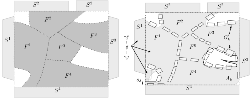
Figure 3. The partition of $A=\bigcup_{i\geq 0}F^{i}$ and the construction of $B_{k}^{\delta}:=A_{k}\setminus G_{k}^{\delta}$ in Proposition 5.1. The set $G_{\delta,k}$ is a finite union of holes along the boundaries $F^{i}\cup\bigcup_{j\neq i}S^{j}$ in which $u_{k}-a_{k}^{i}$ converges. Note that the sets $\{F^{i}\setminus G_{k}^{\delta}\}_{i=0}^{m}$ partition $B_{k}^{\delta}.$ Since $F^{0}$ is a “hanging” component of $A,$ i.e., not linked to the substrate, and hence, it is reasonable to assume that the elastic energy in $F^{0}$ is $0.$ Then we define the displacement fields $v_{k}^{\delta}$ as follows: in $S^{i}\cup(F^{i}\setminus G_{k}^{\delta})$ for $i=1,\ldots,m$ we set $v_{k}^{\delta}:=u_{k}-a_{k}^{i}$ and in $F^{0}\setminus G_{k}^{\delta}$ we write $v_{k}^{\delta}:=u_{0}.$ Finally, since $A_{k}\setminus A$ may present large trace portions along $\partial S$ on which $v_{k}^{\delta}$ forms a jump, we need to change the values of $v_{k}^{\delta}$ in $R_{\delta}^{i}\setminus A$ near $S^{i}.$

We postpone the proof of Proposition 5.1 after the proof of Theorem 2.6.

Proof of Theorem 2.6.

Since $S$ is Lipschitz open set with finitely many connected components, applying the Poincaré-Korn inequality and the Rellich-Kondrachov compactness theorem we find a not relabelled subsequence $\{(A_{k},u_{k})\},$ a partition $\{S^{i}\}_{i=1}^{m}$ of $S$ and $m$ sequences $\{a_{k}^{1}\},\ldots,\{a_{k}^{m}\}$ of rigid displacements such that

• each $S^{i}$ is the union of some connected components of $S$ and $S=\bigcup_{i=1}^{m}S^{i};$

• for each $i\in\{1,\ldots,m\}$ there exists $w^{i}\in H^{1}(S^{i})$ such that $u_{k}-a_{k}^{i}$ converges to $w^{i}$ weakly in $H^{1}(S^{i})$ and a.e. in $S^{i};$

• if $i\neq j,$ then $|a_{k}^{i}-a_{k}^{j}|\to+\infty$ a.e.  in $\mathbb{R}^{n}.$

We may also assume $A_{k}\to A$ in $L^{1}(\mathbb{R}^{n})$ for some $A\in BV(\Omega;\{0,1\}).$ Since $\mathcal{E}v=\mathcal{E}(v+a)$ for any rigid displacement $a$, by Remark 2.3 we have

$$\sup_{k\geq 1}\Big{(}P(A_{k})+\mathcal{H}^{n-1}(J_{(u_{k}-a_{k}^{i})\chi_{A_{k}\cup S}})+\int_{A_{k}\cup S}|\mathcal{E}(u_{k}-a_{k}^{i})|^{2}\mathrm{d}x\Big{)}<+\infty$$

for any $i.$ Hence, by [14, Theorem 1.1] there exist a not relabelled subsequence $\{(A_{k},u_{k})\}$ such that for each $i$ the set

$$F_{i}:=\{x\in\Omega:\,\,\limsup\limits_{k\to+\infty}|(u_{k}(x)-a_{k}^{i}(x))\chi_{A_{k}}(x)|=+\infty\}$$

has finite perimeter and there exists a function $u^{i}\in GSBD^{2}({\rm Int}{(\Omega\cup S\cup\Sigma)})$ such that

$$u_{k}-a_{k}^{i}\to u^{i}\quad\text{a.e.\ in $S^{i}\cup F^{i},$}$$

where

$$F^{i}:=A\setminus F_{i}.$$

By assumption ($\rm a_{3}$) the sets $F^{1},\ldots,F^{m}$ are pairwise disjoint (see Figure 3).

Let $\delta_{0}:=2^{-10}\min_{i\neq j}\{1,\mathrm{dist}(S^{i},S^{j})\}$ and consider any sequence $\delta_{l}\searrow 0$ with $\delta_{1}<\delta_{0}.$ By Proposition 5.1 for any $l\geq 1$ there exists a subsequence $\{(A_{k,l},u_{k,l})\}_{k}\subset\{(A_{k,l-1},u_{k,l-1})\}_{k},$ $k_{\delta_{l}}>0,$ $s_{\delta_{l}}\in(0,\delta_{l})$ and a sequence $\{G_{k}^{\delta_{l}}\}_{k}$ of sets of finite perimeter satisfying (5.1a)-(5.1d) with $\delta=\delta_{l}$ such that the sequence $\{(B_{k}^{\delta_{l}},v_{k}^{\delta_{l}})\}_{k},$ defined as (5.2)-(5.3), satisfies

$$\mathcal{S}(A_{k,l},u_{k,l})\geq\mathcal{S}(B_{k}^{\delta_{l}},v_{k}^{\delta_{l}})-c^{*}\sqrt{\delta_{l}}\Big{[}1+P(A_{k,l})+\mathcal{H}^{n-1}(J_{u_{k,l}})+\sum\limits_{i=0}^{m}\mathcal{H}^{n-1}(\partial^{*}F^{i})\Big{]}$$ (5.5)

for all $k>k_{\delta_{l}}.$ Here we set $(A_{k,0},u_{k,0})=(A_{k},u_{k}).$ By (5.1d) we may also assume that $G_{k}^{\delta_{l}}\to G^{\delta_{l}}$ in $L^{1}(\mathbb{R}^{n})$ as $k\to+\infty,$ and therefore, $B_{k}^{\delta_{l}}\to A\setminus G^{\delta_{l}}.$ Moreover, setting $v_{k}^{\delta_{l}}=\xi$ in $\Omega\setminus B_{k}^{\delta_{l}}$ and $B_{k}^{\delta_{l}}\setminus[\cup_{i}R_{\delta_{l}}^{i}\cup A]$ for some $\xi\in(0,1)^{n}\setminus\Xi_{\{B_{k}^{\delta_{l}},u_{k}^{\delta_{l}}\}_{k,l}}$ (see Remark 2.1), by the choice of $a_{k}^{i}$ we get $v_{k}^{\delta_{l}}\to v^{\delta_{l}}$ a.e.  in $\Omega\cup S,$ where

$$v^{\delta_{l}}:=\sum\limits_{i=1}^{m}u^{i}\chi_{S^{i}\cup(F^{i}\setminus G^{\delta_{l}})}+u_{0}\chi_{F^{0}\setminus G^{1/l}}+\xi\chi_{(\Omega\setminus A)\cup G^{1/l}}.$$

By (5.1c)-(5.1d)

$$|G^{\delta_{l}}|\leq c^{*}\sqrt{\delta_{l}}\sum_{i=0}^{m}P(F^{i}),\qquad P(G^{\delta_{l}})\leq c^{*}\sum_{i=0}^{m}P(F^{i}),$$

and hence, $G^{\delta_{l}}\to\emptyset$ in $L^{1}(\mathbb{R}^{n})$ as $l\to+\infty.$ Therefore, $v^{\delta_{l}}\to u$ a.e.  in $\Omega\cup S$ as $l\to+\infty,$ where

$$u:=\sum\limits_{i=1}^{m}u^{i}\chi_{S^{i}\cup F^{i}}+u_{0}\chi_{F^{0}}+\xi\chi_{\Omega\setminus A}.$$

By the nonnegativity and invariance w.r.t. rigid displacements of the elastic energy we have also

$$\mathcal{W}(A_{k,l},u_{k,l})\geq\mathcal{W}(B_{k}^{\delta_{l}},v_{k}^{\delta_{l}}).$$ (5.6)

For each $l\geq 1$ let us choose $k_{l}>k_{\delta_{l}}$ and consider the sequences $\{(A_{k_{l},l},u_{k_{l},l})\}_{l}$ and let $(B_{l},v_{l}):=(B_{k_{l}}^{l},u_{k_{l}}^{l}).$ We may also assume that $l\mapsto k_{l}$ is strictly increasing. By construction and the definition of $u,$ one readily check that $(B_{l},v_{l})\overset{\tau_{\mathcal{C}}}{\longrightarrow}(A,u).$ Moreover, by construction and (5.1c) $|A_{k_{l},l}\Delta B_{l}|=|G_{k_{l}}^{\delta_{l}}|\to 0.$ Finally, from (5.5) and (5.6) we immediately get

$$\liminf\limits_{l\to+\infty}\mathcal{F}(A_{k_{l},l},u_{k_{l},l})\geq\liminf\limits_{l\to+\infty}\mathcal{F}(B_{l},u_{l}).$$

Thus, the subsequence $\{(A_{k_{l},l},u_{k_{l},l})\}_{l},$ the sequence $\{(B_{l},u_{l})\}$ and the configuration $(A,u)$ satisfy the assertions of Theorem 2.6. ∎

Note that by construction $|B_{l}|\leq|A_{k_{l}}|$ and hence, in general our technique does not imply the compactness of energy-equibounded sequences $\{(A_{k},u_{k})\}$ satisfying a volume constraint.

5.1. Proof of Proposition 5.1

We start with the following estimates near the points of reduced boundary of $A$ (in Proposition 5.1).

Proposition 5.2.

Let $\delta\in(0,1/8),$ $U\subset\mathbb{R}^{n}$ be an open set, $E_{k},E\in BV(U;\{0,1\}),$ and $Q_{r,\nu}(x_{0})\subset\subset U,$ $r>0,$ $\nu\in\mathbb{S}^{n-1},$ be a cube such that

• $x_{0}\in\partial^{*}E,$ $\nu_{E}(x_{0})=\nu$ and

  $$1-\delta<\frac{1}{\phi(\nu)r^{n-1}}\int_{Q_{r,\nu}(x_{0})\cap\partial^{*}E}\phi(\nu_{E})\mathrm{d}\mathcal{H}^{n-1}<1+\delta;$$

• $$\Big{(}\frac{1}{2}-\delta\Big{)}r^{n}<|E\cap Q_{r,\nu}^{-}(x_{0})|,|E\cap Q_{r,\nu}^{+}(x_{0})|<\Big{(}\frac{1}{2}+\delta\Big{)}r^{n},$$

  where $Q_{r,\nu}^{\pm}(x_{0})=\{x\in Q_{r,\nu}(x_{0}):\,\,(x-x_{0})\cdot\nu\gtrless 0\};$

• $E_{k}\to E$ in $L^{1}(U).$

We also denote by $\phi$ a norm in $\mathbb{R}^{n}$ satisfying (4.1). Then there exists $k_{\delta}>0$ such that for any $k>k_{\delta}$ there is $t_{k}^{\delta}\in(\sqrt{\delta},2\sqrt{\delta})$ such that $\mathcal{H}^{n-1}(T_{t_{k}^{\delta}r}\cap\partial^{*}E_{k})=0$ and

$$\mathcal{H}^{n-1}(T_{t_{k}^{\delta}r}\cap E_{k}^{(1)})+\mathcal{H}^{n-1}(T_{-t_{k}^{\delta}r}\cap(Q_{1}^{-}\setminus E^{(1)}))+\mathcal{H}^{n-1}(T_{-t_{k}^{\delta}r}\cap(E_{k}^{(1)}\Delta E^{(1)}))<4\sqrt{\delta}r^{n-1},$$

where

$$T_{t}:=\{x\in Q_{r,\nu}(x_{0}):\,\,(x-x_{0})\cdot\nu=t\},\quad t\in(-r,r),$$

and the set

$$D_{k}^{\delta}:=Q_{r,\nu}(x_{0})\cap\{|(x-x_{0})\cdot\nu|<t_{k}^{\delta}r\}$$

satisfies

$$\int_{D_{k}^{\delta}\cap\partial^{*}E_{k}}\phi(\nu_{E_{k}})\mathrm{d}\mathcal{H}^{n-1}\geq \phi(\nu)\mathcal{H}^{n-1}(T_{-t_{k}^{\delta}r})-(4n+12)b_{2}\sqrt{\delta}r^{n-1}.$$

(see Figure 4).

In the proof of Proposition 5.1 we apply this proposition with $U=\Omega,$ $E_{k}:=A_{k}$ and $E=A.$

Figure 4. The sets $E_{k}$ and $E$ in Proposition 5.2.

Proof.

Without loss of generality we assume that $x_{0}=0,$ $\nu={\bf e}_{n}$ and $r=1.$ By (a2)

$$|Q_{1}^{+}\cap E|\leq|E|-|E\cap Q_{1}^{-}|<2\delta,$$

and hence, by (a3) there exists $k_{\delta}>0$ such that

$$|Q_{1}^{+}\cap E_{k}|<2\delta\quad\text{and}\quad|E_{k}\Delta E|<\delta\quad\text{for all $k>k_{\delta}.$ }$$ (5.7)

Also by (a2)

$$|Q_{1}^{-}\setminus E|\leq|Q_{1}^{-}|-|Q_{1}^{-}\cap E|<\delta,$$

thus, by (5.7) and the coarea formula

$$4\delta>|Q_{1}^{+}\cap E_{k}|+|Q_{1}^{-}\setminus E|+|E_{k}\Delta E|=\int_{0}^{1/2}\Big{[}\mathcal{H}^{n-1}(T_{t}\cap E_{k}^{(1)})+\mathcal{H}^{n-1}(T_{-t}\cap[Q_{1}^{-}\setminus E^{(1)}])\\ +\mathcal{H}^{n-1}(T_{t}\cap[E_{k}^{(1)}\Delta E^{(1)}])+\mathcal{H}^{n-1}(T_{-t}\cap[E_{k}^{(1)}\Delta E^{(1)}])\Big{]}\mathrm{d}t.$$

In particular there exists $t_{k}^{\delta}\in(\sqrt{\delta},2\sqrt{\delta})$ such that

$$\mathcal{H}^{n-1}(T_{t_{k}^{\delta}}\cap E_{k}^{(1)})+\mathcal{H}^{n-1}(T_{-t_{k}^{\delta}}\cap(Q_{1}^{-}\setminus E^{(1)}))+\mathcal{H}^{n-1}(T_{-t_{k}^{\delta}}\cap(E_{k}^{(1)}\Delta E^{(1)}))<4\sqrt{\delta}.$$ (5.8)

Define

$$D_{k}^{\delta}:=\big{(}-1/2,1/2\big{)}^{n-1}\times(-t_{k}^{\delta},t_{k}^{\delta})$$

(see Figure 4). Note that

$$\int_{D_{k}^{\delta}\cap\partial^{*}E_{k}}\phi(\nu_{E_{k}})\mathrm{d}\mathcal{H}^{n-1}=\int_{\{x\cdot{\bf e}_{n}>-t_{k}^{\delta}\}\cap\partial^{*}(D_{k}^{\delta}\cap E_{k})}\phi(\nu_{D_{k}^{\delta}\cap E_{k}})\mathrm{d}\mathcal{H}^{n-1}\\ -\int_{\partial^{*}E_{k}\cap\overline{D_{k}^{\delta}}\cap\partial Q_{1}}\phi(\nu_{Q_{1}})\mathcal{H}^{n-1}-\int_{E_{k}^{(1)}\cap T_{t_{k}^{\delta}}}\phi({\bf e}_{n})\mathcal{H}^{n-1}.$$

By the choice (5.8) of $t_{k}^{\delta}$

$$\int_{E_{k}^{(1)}\cap T_{t_{k}^{\delta}}}\phi({\bf e}_{n})\mathcal{H}^{n-1}\leq b_{2}\mathcal{H}^{n-1}(E_{k}^{(1)}\cap T_{t_{k}^{\delta}})<4b_{2}\sqrt{\delta}$$

and

$$\int_{\partial^{*}E_{k}\cap\overline{D_{k}^{\delta}}\cap\partial Q_{1}}\phi(\nu_{Q_{1}})\mathcal{H}^{n-1}\leq b_{2}\mathcal{H}^{n-1}(\partial D_{k}^{\delta}\cap\partial Q_{1})<4(n-1)b_{2}\sqrt{\delta},$$

where $2(n-1)$ is the perimeter of $(-1/2,1/2)^{n-1}.$ Moreover, by the anisotropic (local) minimality of half-spaces (see e.g. [7, Example 2.4])

$$\int_{\{x\cdot{\bf e}_{n}>-t_{k}^{\delta}\}\cap\partial^{*}(D_{k}\cap E_{k})}\phi(\nu_{D_{k}\cap E_{k}})\mathrm{d}\mathcal{H}^{n-1}\geq\phi({\bf e}_{n})\mathcal{H}^{n-1}(E_{k}^{(1)}\cap T_{-t_{k}^{\delta}}),$$

and hence, by (5.8) (we can replace $E_{k}$ with $E$)

$$\int_{\{x\cdot{\bf e}_{n}>-t_{k}^{\delta}\}\cap\partial^{*}(D_{k}\cap E_{k})}\phi(\nu_{D_{k}\cap E_{k}})\mathrm{d}\mathcal{H}^{n-1}\geq\phi({\bf e}_{n})\mathcal{H}^{n-1}(E^{(1)}\cap T_{-t_{k}^{\delta}})-4b_{2}\sqrt{\delta}.$$

Again by (5.8)

$$\mathcal{H}^{n-1}(E^{(1)}\cap T_{-t_{k}^{\delta}})=\mathcal{H}^{n-1}(T_{-t_{k}^{\delta}})-\mathcal{H}^{n-1}((Q_{1}^{-}\setminus E^{(1)})\cap T_{-t_{k}^{\delta}})>\mathcal{H}^{n-1}(T_{-t_{k}^{\delta}})-4\sqrt{\delta}$$

and therefore,

$$\int_{D_{k}^{\delta}\cap\partial^{*}E_{k}}\phi(\nu_{E_{k}})\mathrm{d}\mathcal{H}^{n-1}\geq\phi({\bf e}_{n})\mathcal{H}^{n-1}(T_{-t_{k}^{\delta}})-4(n+3)b_{2}\sqrt{\delta}.$$

∎

Now applying Proposition 4.1 and 5.2 we construct the set $G_{k}^{\delta}$ in Proposition 5.1.

Proof of Proposition 5.1.

Without loss of generality we assume $u_{k}=\xi$ in $\Omega\setminus A_{k}$ for some $\xi\in(0,1)^{n}\setminus\Xi_{\{(A_{k},u_{k})\}\}}$ (see Remark 2.1).

By the uniform continuity of $\varphi,$ there exists $r_{\delta}\in(0,1)$ such that

$$|\varphi(x,\nu)-\varphi(y,\nu)|<\delta\quad\text{for all $x,y\in\overline{\Omega}$ with $|x-y|<r_{\delta}.$}$$ (5.9)

Let

$$\widetilde{K}_{1}:= \Sigma\cap\partial^{*}A\cap\bigcup_{i=1}^{m}\Big{(}\partial S^{i}\cap\bigcup_{j\neq i}\partial^{*}F^{j}\Big{)},$$

$$\widetilde{K}_{2}:= \Omega\cap A^{(1)}\cap\bigcup_{i=0}^{m}\partial^{*}F^{i},$$

$$\widetilde{K}_{3}:= \Omega\cap\partial^{*}A\cap\bigcup_{i=0}^{m}\partial^{*}F^{i}.$$

Since these sets are $\mathcal{H}^{n-1}$-rectifiable and pairwise disjoint, (by a simple covering argument) we can find open sets $U_{1}\subset\subset{\rm Int}{(\Omega\cup S\cup\Sigma)}$ and $U_{2},U_{3}\subset\subset\Omega$ with disjoint closures such that

$$\sum\limits_{i=1}^{3}\mathcal{H}^{n-1}\big{(}\widetilde{K}_{i}\setminus U_{i}\big{)}+\sum\limits_{i=1}^{3}\mathcal{H}^{n-1}\Big{(}\widetilde{K}_{i}\cap\bigcup_{j\neq i}U_{j}\Big{)}<\delta.$$ (5.10)

Set

$$K_{i}:=U_{i}\cap\widetilde{K}_{i},\quad i=1,2,3.$$

Note that around $\mathcal{H}^{n-1}$-a.e.  point of $\cup_{i}K_{i}$ there exist $j\in\{1,\ldots,m\}$ and a cube $Q$ such that $\cup_{i}K_{i}$ “roughly divides” $Q$ into two parts in one $u_{k}-a_{k}^{j}$ converges and in the other either $u_{k}$ is constant or $|u_{k}-a_{k}^{j}|\to+\infty.$ For convenience of the reader we divide the construction of $G_{k}^{\delta}$ into smaller steps.

Step 1. Using the $\mathcal{H}^{n-1}$-rectifiability of $K_{i},$ $\partial^{*}A,$ $\partial^{*}F^{i},$ the lipschitzianity of $\Sigma$ and the Borel regularity of corresponding unit normals we construct a fine cover of $\cup_{i}K_{i}$ as follows.

Substep 1.1: fine cover for $K_{1}.$ For $\mathcal{H}^{n-1}$-a.e.  $x\in K_{1}$ there exist $i_{x},j_{x}\in\{1,\ldots,m\}$ with $i_{x}\neq j_{x}$ and $r_{x}>0$ such that $x\in(\partial S^{i_{x}}\setminus\partial^{*}F^{i_{x}})\cap\partial^{*}F^{j_{x}}$ and:

• $r_{x}<\frac{1}{4}\min\{r_{\delta},\mathrm{dist}(x,\partial U_{1})\},$ where $r_{\delta}$ is defined in (5.9);

• $\theta(\Sigma,x)=\theta(K_{1},x)=\theta(\partial^{*}F^{j_{x}},x)=\theta(\partial^{*}A,x)=1$ and $\nu_{\Sigma}(x),$ $\nu_{K_{1}}(x),$ $\nu_{F^{j_{x}}}(x)$ and $\nu_{A}(x)$ exist and are parallel each other. For shortness, we set $\nu_{x}:=\nu_{\Sigma}(x);$

• $\Gamma_{x}:=Q_{r_{x},\nu_{x}}(x)\cap\Sigma$ separates $Q_{r_{x},\nu_{x}}(x)$ into two connected components;

• for any $r\in(0,r_{x})$

  $$|\nu_{\Gamma_{x}}(y)-\nu_{x}|<\delta\quad\text{and}\quad|(y-x)\cdot\nu_{x}|<\tfrac{\delta r}{2}\quad\text{for all $y\in\Gamma_{x},$}$$ (5.11a)

  $$(1-\delta)r^{n-1}<\mathcal{H}^{n-1}(Q_{r}\cap\Gamma_{x}\cap\partial^{*}F^{j_{x}})\leq\mathcal{H}^{n-1}(Q_{r}\cap\Gamma_{x})<(1+\delta)r^{n-1},$$ (5.11b)

  $$\mathcal{H}^{n-1}\Big{(}\Big{[}Q_{r}\cap\bigcup_{j=0}^{m}\partial^{*}F^{j}\Big{]}\setminus\Gamma_{x}\Big{)}+\mathcal{H}^{n-1}(Q_{r}\cap[\partial^{*}F^{j_{x}}\Delta\Gamma_{x}])<\delta r^{n-1},$$ (5.11c)

  $$|(F^{j_{x}}\cup S)\cap Q_{r}|\geq(1-\delta)r^{n},$$ (5.11d)

  where $Q_{r}:=Q_{r,\nu_{x}}(x).$

Removing an $\mathcal{H}^{n-1}$-negligible set from $K_{1}$ if necessary we assume that for all points $x\in K_{1}$ there exist $r_{x}$ and $i_{x},j_{x}$ satisfying ($a_{1.1}$)-($a_{1.4}$).

Let us show that for any $x\in K_{1}$ and $r\in(0,r_{x})$, the cube $Q_{r,\nu_{x}}(x)$, the sequence $\{(A_{k},u_{k}-a_{k}^{j_{x}})\},$ the configuration $(A,u^{j_{x}})$, conditions ($\rm a_{1.1}$)-($\rm a_{1.4}$), the sets $E:=Q_{r_{x},\nu_{x}}(x)\setminus F^{j_{x}}$ and $K:=Q_{r_{x},\nu_{x}}(x)\cap\partial^{*}F^{j_{x}}$ satisfy all assumptions of Proposition 4.1. Indeed, conditions for $\Gamma$ follow from ($\rm a_{1.3}$), (5.11a) and (5.11b), while conditions (a3)-(a4) for $\{(A_{k},u_{k})\}$ follows from our assumption in the beginning of the proof and the assumption of Proposition 5.1. The definition of $F^{j_{x}}$ implies condition (a6) with $E:=Q_{r_{x},\nu_{x}}(x)\setminus F^{j_{x}}$ and $K:=Q_{r_{x},\nu_{x}}(x)\cap\partial^{*}F^{j_{x}}.$ Finally, the estimates (5.11b) and (5.11c) together with ($\rm a_{1.2}$) yield that $A\cup S$ and $K$ satisfy conditions (a5) and (a7), respectively.

Substep 1.2: fine cover for $K_{2}.$ For $\mathcal{H}^{n-1}$-a.e.  $x\in K_{3}$ there exist $r_{x}>0,$ $i_{x},j_{x}\in\{0,\ldots,m\}$ with $i_{x}\neq j_{x}$ and an $(n-1)$-dimensional $C^{1}$-graph $\Gamma_{x}$ containing $x$ such that

• $r_{x}<\frac{1}{4}\min\{r_{\delta},\mathrm{dist}(x,\partial U_{2})\}.$

• $\theta(K_{2},x)=\theta(\partial^{*}F^{i_{x}},x)=\theta(\partial^{*}F^{j_{x}},x)=\theta(K_{2}\cap\partial^{*}F^{i_{x}}\cap\partial^{*}F^{j_{x}}\cap\Gamma_{x},x)=1$ and unit normals $\nu_{K_{2}},$ $\nu_{F^{i_{x}}}(x)$ and $\nu_{F^{j_{x}}}(x)$ exist and is parallel to $\nu_{x}:=\nu_{\Gamma_{x}}(x);$

• $\Gamma_{x}$ separates $Q_{r_{x},\nu_{x}}(x)$ into two connected components;

• for any $r\in(0,r_{x})$

  $$|\nu_{\Gamma_{x}}(y)-\nu_{x}|<\delta\quad\text{and}\quad|(y-x)\cdot\nu_{x}|<\tfrac{\delta r}{2}\quad\text{for all $y\in\Gamma_{x}\cap Q_{r}$,}$$ (5.12a)

  $$(1-\delta)r^{n-1}<\mathcal{H}^{n-1}(Q_{r}\cap\Gamma_{x}\cap K_{2}\cap\partial^{*}F^{i_{x}}\cap\partial^{*}F^{j_{x}})$$

  $$\hskip 142.26378pt\leq\mathcal{H}^{n-1}(Q_{r}\cap\Gamma_{x})<(1+\delta)r^{n-1},$$ (5.12b)

  $$\mathcal{H}^{n-1}(Q_{r}\cap[\Gamma_{x}\Delta(\partial^{*}F^{i_{x}}\cap\partial^{*}F^{j_{x}})])+\mathcal{H}^{n-1}\Big{(}\Big{[}Q_{r}\cap\bigcup_{j=0}^{N_{2}}\partial^{*}F^{j}\Big{]}\setminus\Gamma_{x}\Big{)}<\delta r^{n-1},$$ (5.12c)

  $$\Big{(}\tfrac{1}{2}-\delta\Big{)}r^{n}\leq|F^{i_{x}}\cap Q_{r}^{-}|,|F^{j_{x}}\cap Q_{r}^{+}|\leq\Big{(}\tfrac{1}{2}+\delta\Big{)}r^{n},$$ (5.12d)

  where $Q_{r}:=Q_{r,\nu_{x}}(x)$ and $Q_{r}^{\pm}:=\{y\in Q_{r}:\,\,(y-x)\cdot\nu_{x}\gtrless 0\}.$ Here the volume density estimates follows from the definition of reduced boundary.

Removing an $\mathcal{H}^{n-1}$-negligible set from $K_{2}$ if necessary we assume that for all points $x\in K_{2}$ there exist $r_{x}$ and $i_{x},j_{x}$ satisfying ($\rm a_{2.1}$)-($\rm a_{2.4}$). Then using $A=\cup_{j=0}^{N_{2}}F^{j}$ and $\partial^{*}A\subset\cup_{j=0}^{N_{2}}\partial^{*}F^{j}$ as in Substep 1.1. one can check that for any $x\in K_{2}$ and $r\in(0,r_{x})$, the cube $Q_{r,\nu_{x}}(x)$, the sequence $\{(A_{k},u_{k}-a_{k}^{i_{x}})\},$ the configuration $(A,u^{i_{x}})$ and the sets $E:=Q_{r_{x},\nu_{x}}(x)\setminus F^{i_{x}}$ and $K=Q_{r_{x},\nu_{x}}(x)\cap\partial^{*}F^{i_{x}}$ satisfy all conditions of Proposition 4.1.

Substep 1.3: fine cover for $K_{3}.$ For $\mathcal{H}^{n-1}$-a.e.  $x\in K_{3}$ there exist $r_{x}>0,$ $i_{x}\in\{0,\ldots,m\}$ and an $(n-1)$-dimensional $C^{1}$-graph $\Gamma_{x}$ containing $x$ such that

• $r_{x}<\frac{1}{4}\min\{r_{\delta},\mathrm{dist}(x,\partial U_{4})\};$

• $\theta(K_{3},x)=\theta(\partial^{*}F^{i_{x}},x)=\theta(\partial^{*}A,x)=\theta(K_{3}\cap\Gamma_{x}\cap\partial^{*}A\cap\partial^{*}F^{i_{x}},x)=1$ and the unit normals $\nu_{K_{3}}(x),$ $\nu_{A}(x)$ and $\nu_{F^{i_{x}}}(x)$ exist and coincide with $\nu_{x}:=\nu_{\Gamma_{x}}(x);$

• $\Gamma_{x}$ separates $Q_{r_{x},\nu_{x}}(x)$ into two connected components;

• for any $r\in(0,r_{x})$

  $$|\nu_{\Gamma_{x}}(y)-\nu_{x}|<\delta\quad\text{and}\quad|(y-x)\cdot\nu_{x}|<\tfrac{\delta r}{2}\quad\text{for all $y\in\Gamma_{x}\cap Q_{r},$}$$ (5.13a)

  $$(1-\delta)r^{n-1}<\mathcal{H}^{n-1}(Q_{r}\cap\Gamma_{x}\cap K_{3}\cap\partial^{*}F^{i_{x}}\cap\partial^{*}A)$$

  $$\hskip 170.71652pt\leq\mathcal{H}^{n-1}(Q_{r}\cap\Gamma_{x})<(1+\delta)r^{n-1},$$ (5.13b)

  $$\mathcal{H}^{n-1}(Q_{r}\cap[\Gamma_{x}\Delta(\partial^{*}F^{i_{x}}\cap\partial^{*}A)])+\mathcal{H}^{n-1}\Big{(}\Big{[}Q_{r}\cap\bigcup_{j=0}^{N_{3}}\partial^{*}F^{i_{x}}\Big{]}\setminus\Gamma_{x}\Big{)}<\delta r^{n-1},$$ (5.13c)

  $$(1-\delta)r^{n-1}<\frac{1}{\varphi(x,\nu_{x})}\,\int_{Q_{r}\cap\partial^{*}F^{i_{x}}}\varphi(x,\nu_{F^{i_{x}}}(y))\mathrm{d}\mathcal{H}^{n-1}(y)$$ (5.13d)

  $$\hskip 85.35826pt\leq\frac{1}{\varphi(x,\nu_{x})}\,\int_{Q_{r}\cap\partial^{*}A}\varphi(x,\nu_{A}(y))\mathrm{d}\mathcal{H}^{n-1}(y)<(1+\delta)r^{n-1},$$ (5.13e)

  $$\Big{(}\tfrac{1}{2}-\delta\Big{)}r^{n}<|Q_{r}^{-}\cap F^{i_{x}}|\leq|Q_{r}^{-}\cap A|<\Big{(}\tfrac{1}{2}+\delta\Big{)}r^{n},$$ (5.13f)

  $$|Q_{r}^{+}\cap A|<\delta r^{n},$$ (5.13g)

  where $Q_{r}:=Q_{r,\nu_{x}}(x).$

Removing an $\mathcal{H}^{n-1}$-negligible set from $K_{3}$ if necessary we assume that for all points $x\in K_{3}$ there exists $r_{x}>0$ and $i_{x}$ satisfying ($\rm a_{3.1}$)-($\rm a_{3.4}$). Then for any $x\in K_{3}$ and $r\in(0,r_{x})$ the set $U=U_{3},$ the cube $Q_{r,\nu_{x}}(x),$ the sequence $E_{k}:=Q_{r,\nu_{x}}(x)\cap A_{k},$ the set $E:=Q_{r,\nu_{x}}(x)\cap A$ and conditions ($\rm a_{3.1}$)-($\rm a_{3.4}$) satisfy all assumptions of Proposition 5.2. Indeed, conditions (a1)-(a2) are given in (5.13e) and (5.13f), whereas (a3) follows from the assumption $A_{K}\to A$ in $L^{1}(\mathbb{R}^{n})$ as $k\to+\infty.$

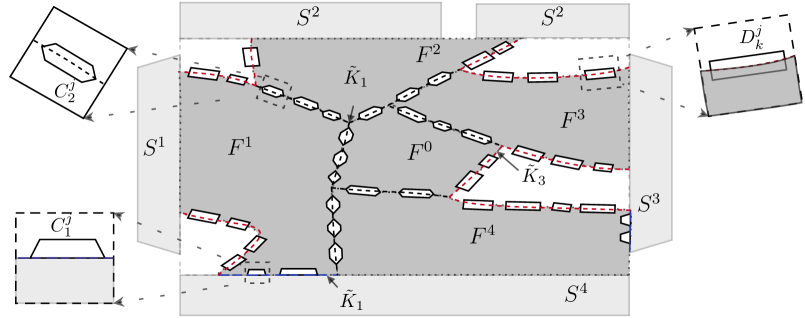
Figure 5. Construction of holes $C_{1}^{j},$ $C_{2}^{j}$ and $D_{k}^{j}.$

Step 2. Now we extract finitely many covering cubes still covering $\cup_{i}K_{i}$ up to some error of order $O(\sqrt{\delta}),$ and create “holes” inside those cubes (i.e., the sets $C_{1}^{j},$ $C_{2}^{j}$ and $D_{k}^{j}$ in Figure 5). By Step 1, for each $i\in\{1,2,3\}$ the collection $\{\overline{Q_{r,\nu_{x}}(x)}:\,\,x\in K_{i},\,\,r\in(0,r_{x})\}$ of cubes provides a fine cover for $K_{i}$ and hence, by the Vitali covering lemma we can extract an at most countable pairwise disjoint family $\{Q_{r_{j}^{i},\nu_{x_{j}^{i}}}(x_{j}^{i}),\,x_{j}^{i}\in K_{i}\}$ such that

$$\mathcal{H}^{n-1}\Big{(}K_{i}\setminus\bigcup_{j}Q_{r_{j}^{i},\nu_{x_{j}^{i}}}(x_{j}^{i})\Big{)}=0.$$

Since $\mathcal{H}^{n-1}(K_{i})<+\infty$, there exists $N_{i}\geq 1$ such that

$$\mathcal{H}^{n-1}\Big{(}K_{i}\setminus\bigcup_{j>N_{i}}Q_{r_{j}^{i},\nu_{x_{j}^{i}}}(x_{j}^{i})\Big{)}<\delta.$$ (5.14)

Moreover, decreasing $r_{j}$ a bit necessary, we assume that $\overline{Q_{r_{j}^{i},\nu_{x_{j}^{i}}}(x_{j}^{i})}\cap\overline{Q_{r_{j^{\prime}}^{i},\nu_{x_{j^{\prime}}^{i}}}(x_{j^{\prime}}^{i})}=\emptyset$ for all $1\leq j<j^{\prime}\leq N_{i}.$ Since $\overline{U_{i}}\cap\overline{U_{j}}=\emptyset$ for $i\neq j,$ cubes belonging to the union of $\mathcal{G}_{i}:=\{Q_{r_{j}^{i},\nu_{x_{j}^{i}}}(x_{j}^{i})\}_{j=1}^{N_{i}},$ $i=1,2,3,$ have disjoint closures. When no confusion arises, we drop the dependence of $x_{j}^{i}$ and $r_{j}^{i}$ on $i.$

Substep 2.1: definition of $C_{1}^{j}.$ Let $Q_{r_{j},x_{j}}(x_{j})\in\mathcal{G}_{1}$ for some $j\in\{1,\ldots,N_{1}\}.$ By Substep 1.1 $x_{j}\in K_{1}\cap\partial S^{l_{j}}\cap\partial^{*}F^{h_{j}}$ for some $l_{j},h_{j}\in\{1,\ldots,m\}$ with $l_{j}\neq h_{j}.$ Applying Proposition 4.1 (ii) with $Q_{r_{j},\nu_{x_{j}}}(x_{j})\subset\subset{\rm Int}{(\Omega\cup S\cup\Sigma)},$ $\Gamma_{x_{j}}:=Q_{r_{j},\nu_{x_{j}}}(x_{j})\cap\Sigma,$ $\{(A_{k},u_{k}-a_{k}^{h_{j}})\},$ $(A,u^{h_{j}}),$ $E:=Q_{r_{j},\nu_{x_{j}}}(x_{j})\setminus F^{h_{j}},$ $K:=Q_{r_{j},\nu_{x_{j}}}(x_{j})\cap\partial^{*}F^{h_{j}}$ and $\phi(\cdot)=\varphi(x_{j},\cdot)$ we find an open set $C_{1}^{j}\subset\Omega\cap Q_{r_{j},\nu_{x_{j}}}(x_{j})$ of finite perimeter (given by Lemma 3.1) and $k_{\delta}^{1,j}>0$ such that

$$\int_{C_{1}^{j}\cap\partial^{*}A_{k}}\phi(\nu_{A_{k}})\mathrm{d}\mathcal{H}^{n-1}+2\int_{C_{1}^{j}\cap A_{k}^{(1)}\cap J_{u_{k}}}\phi(\nu_{J_{u_{k}}}) \mathrm{d}\mathcal{H}^{n-1}+2\int_{\Sigma\cap\partial^{*}C_{1}^{j}\cap\partial^{*}A_{k}\cap J_{u_{k}}}\phi(\nu_{J_{u_{k}}})\mathrm{d}\mathcal{H}^{n-1}$$

$$\geq 2\int_{Q_{r_{j},\nu_{j}}(x_{j})\cap\partial^{*}F^{h_{j}}}\phi(\nu_{F^{h_{j}}})\mathrm{d}\mathcal{H}^{n-1}-c^{\prime}\delta r_{j}^{n-1}$$

$$\geq \int_{\partial^{*}C_{1}^{j}}\phi(\nu_{C_{1}^{j}})\mathrm{d}\mathcal{H}^{n-1}-(c^{\prime}+5b_{2})\delta r_{j}^{n-1}$$ (5.15)

for all $k>k_{\delta}^{1,j}$ and for some $c^{\prime}>0$ (depending only on $b_{2}$).

Let us estimate the perimeter and the volume of $\cup_{j}C_{1}^{j}.$ By (5.11b)

$$r_{j}^{n-1}\leq\frac{1}{1-\delta}\mathcal{H}^{n-1}(Q_{r_{j},\nu_{j}}\cap\Sigma\cap\partial^{*}F^{h_{j}})$$ (5.16)

and hence, by (2.8) and (3.2)

$$b_{1}\mathcal{H}^{n-1}(\partial^{*}C_{1}^{j})\leq \int_{\partial^{*}C_{1}^{j}}\phi(\nu_{C_{1}^{j}})\mathrm{d}\mathcal{H}^{n-1}\leq 2\int_{Q_{r_{j},\nu_{j}}(x_{j})\cap\partial^{*}F^{h_{j}}}\phi(\nu_{F^{h_{j}}})\mathrm{d}\mathcal{H}^{n-1}+5b_{2}\delta r_{j}^{n-1}$$

$$\leq 2b_{2}\mathcal{H}^{n-1}(Q_{r_{j},\nu_{j}}(x_{j})\cap\partial^{*}F^{h_{j}})+5b_{2}\delta r_{j}^{n-1}$$

so that

$$\mathcal{H}^{n-1}(\partial^{*}C_{1}^{j})\leq\frac{3b_{2}}{b_{1}}\mathcal{H}^{n-1}(Q_{r_{j},\nu_{j}}(x_{j})\cap\partial^{*}F^{h_{j}}).$$ (5.17)

Moreover,

$$|C_{1}^{j}|\leq\delta r_{j}^{n}<\delta r_{j}^{n-1}\leq 2\delta\mathcal{H}^{n-1}(Q_{r_{j},\nu_{j}}(x_{j})\cap\Sigma\cap\partial^{*}F^{h_{j}})$$

and therefore,

$$\Big{|}\bigcup_{j=1}^{N_{i}}C_{1}^{j}\Big{|}\leq 2\delta\sum\limits_{h=1}^{m}\mathcal{H}^{n-1}(\partial^{*}F^{h}).$$ (5.18)

Let us estimate the error in covering $K_{1}$ by $\{C_{1}^{j}\}.$ Fix some $j\in\{1,\ldots,N_{1}\}.$ Then by the definition of $K_{1},$ the error estimate (5.11c) and Lemma 3.1 (ii)

$$\mathcal{H}^{n-1}((Q_{r_{j},\nu_{x_{j}}}(x_{j})\cap K_{1})\setminus\overline{C_{1}^{j}})\leq\mathcal{H}^{n-1}\Big{(}\Big{[}Q_{r_{j},\nu_{x_{j}}}(x_{j})\cap\bigcup_{j=0}^{N_{1}}\partial^{*}F^{j}\Big{]}\setminus\Gamma_{x_{j}}\Big{)}+\mathcal{H}^{n-1}(\Gamma_{x_{j}}\setminus\partial^{*}F^{h_{j}})\\ +\mathcal{H}^{n-1}([Q_{r_{j},\nu_{x_{j}}}(x_{j})\cap\partial^{*}F^{h_{j}}]\setminus\overline{C_{1}^{j}})<3\delta r_{j}^{n-1}$$

and thus, by (5.16) and the choice $\delta<1/8$

$$\mathcal{H}^{n-1}((Q_{r_{j},\nu_{x_{j}}}(x_{j})\cap K_{1})\setminus\overline{C_{1}^{j}})<4\delta\,\mathcal{H}^{n-1}(Q_{r_{j},\nu_{x_{j}}}(x_{j})\cap\Sigma\cap\partial^{*}F^{h_{j}}).$$ (5.19)

From (5.14) and (5.19) it follows that

$$\mathcal{H}^{n-1}\Big{(}K_{1}\setminus\bigcup_{j=1}^{N_{1}}\overline{C_{1}^{j}}\Big{)}= \mathcal{H}^{n-1}\Big{(}K_{1}\setminus\bigcup_{j>N_{1}}Q_{r_{j},\nu_{j}}(x_{j})\Big{)}+\sum\limits_{j=1}^{N_{1}}\mathcal{H}^{n-1}([Q_{r_{j},\nu_{x_{j}}}(x_{j})\cap K_{1}]\setminus\overline{C_{1}^{j}})$$

$$< \delta+4\delta\sum_{j=1}^{N_{1}}\mathcal{H}^{n-1}(Q_{r_{j},\nu_{x_{j}}}(x_{j})\cap\Sigma\cap\partial^{*}F^{h_{j}})$$

so that by the disjointness of $\{F^{h}\}$

$$\mathcal{H}^{n-1}\Big{(}K_{1}\setminus\bigcup_{j=1}^{N_{1}}\overline{C_{1}^{j}}\Big{)}<\delta+4\delta\sum\limits_{h=1}^{m}\mathcal{H}^{n-1}(\partial^{*}F^{h}).$$ (5.20)

Substep 2.2: construction of $C_{2}^{j}$. Let $Q_{r_{j},\nu_{j}}(x_{j})\in\mathcal{G}_{2}$ for some $j\in\{1,\ldots,N_{2}\}$ so that there exist $l_{j},h_{j}\in\{0,\ldots,m\}$ with $l_{j}\neq h_{j}\neq 0$ such that $x_{j}\in\partial^{*}F^{l_{j}}\cap\partial^{*}F^{h_{j}}.$ As in Substep 2.1 applying Proposition 4.1 with $Q_{r_{j},\nu_{x_{j}}}(x_{j})\subset\subset\Omega,$ $\Gamma_{x_{j}},$ $\{(A_{k},u_{k}-a_{k}^{h_{j}})\},$ $(A,u^{h_{j}}),$ $E:=Q_{r_{j},\nu_{j}}(x_{j})\setminus F^{h_{j}},$ $K:=Q_{r_{j},\nu_{j}}(x_{j})\cap\partial^{*}F^{h_{j}}$ and $\phi(\cdot)=\varphi(x_{j},\cdot)$ we find an open set $C_{2}^{j}\subset\subset Q_{r_{j},\nu_{x_{j}}}(x_{j})$ of finite perimeter (given by Lemma 3.1) and $k_{\delta}^{2,j}>0$ such that

$$\int_{C_{2}^{j}\cap\partial^{*}A_{k}}\phi(\nu_{A_{k}})\mathrm{d}\mathcal{H}^{n-1}+2\int_{C_{2}^{j}\cap A_{k}^{(1)}\cap J_{u_{k}}}\phi(\nu_{J_{u_{k}}})\mathrm{d}\mathcal{H}^{n-1}\geq\int_{\partial C_{2}^{j}}\phi(\nu_{C_{2}^{j}})\mathrm{d}\mathcal{H}^{n-1}-c^{\prime}\delta r_{j}^{n-1}$$ (5.21)

for all $k>k_{\delta}^{2,j},$ where $c^{\prime}$ depends only on $b_{2}.$ As in Substep 2.1, by (5.12b)

$$r_{j}^{n-1}\leq\frac{1}{1-\delta}\mathcal{H}^{n-1}(Q_{r_{j},\nu_{j}}(x_{j})\cap\partial^{*}F^{l_{j}}\cap\partial^{*}F^{h_{j}})$$ (5.22)

by (2.8) and (3.1)

$$\mathcal{H}^{n-1}(\partial^{*}C_{2}^{j})\leq\frac{2b_{2}}{b_{1}}\mathcal{H}^{n-1}(Q_{r_{j},\nu_{j}}(x_{j})\cap\partial^{*}F^{h_{j}})+\frac{5b_{2}}{b_{1}}\,\delta r_{j}^{n-1}\leq\frac{3b_{2}}{b_{1}}\mathcal{H}^{n-1}(Q_{r_{j},\nu_{j}}(x_{j})\cap\partial^{*}F^{h_{j}})$$ (5.23)

and

$$\Big{|}\bigcup_{j=1}^{N_{2}}C_{2}^{j}\Big{|}\leq 2\delta\sum_{h=0}^{m}\mathcal{H}^{n-1}(\partial^{*}F^{h}).$$ (5.24)

Moreover,

$$\mathcal{H}^{n-1}\Big{(}K_{2}\setminus\bigcup_{j=1}^{N_{2}}\overline{C_{2}^{j}}\Big{)}<\delta+4\delta\sum_{h=0}^{m}\mathcal{H}^{n-1}(\partial^{*}F^{h})$$ (5.25)

Substep 2.3: construction of $D_{k}^{j}$. Let $Q_{r_{j},\nu_{j}}(x_{j})\in\mathcal{G}_{3}$ for some $j\in\{1,\ldots,N_{3}\}$ and let $x_{j}\in\partial^{*}F^{h_{j}}\cap\partial^{*}A$ for some $h_{j}\in\{0,\ldots,m\}.$ Using Proposition 5.2 applied with $U:=Q_{r_{j},\nu_{x_{j}}}(x_{j}),$ $E_{k}:=Q_{r_{j},\nu_{x_{j}}}(x_{j})\cap A_{k},$ $E:=Q_{r_{j},\nu_{x_{j}}}(x_{j})\cap A$ and $\phi(\cdot)=\varphi(x_{j},\cdot)$ we find $k_{\delta}^{3,j}>0$ such that for any $k>k_{\delta}^{3,j}$ there exists $t_{k,j}^{\delta}\in(\sqrt{\delta},2\sqrt{\delta})$ such that $\mathcal{H}^{n-1}(\partial^{*}A_{k}\cap T_{t_{k,j}^{\delta},r_{j}}^{j})=0$ and

$$\mathcal{H}^{n-1}(T_{t_{k,j}^{\delta}r_{j}}^{j}\cap A_{k}^{(1)})+\mathcal{H}^{n-1}(T_{-t_{k,j}^{\delta}r_{j}}^{j}\cap [Q_{r_{j},\nu_{j}}^{-}(x_{j})\setminus A^{(1)}])$$

$$+\mathcal{H}^{n-1}(T_{-t_{k,j}^{\delta}r_{j}}^{j}\cap[A_{k}^{(1)}\Delta A^{(1)}])<4\sqrt{\delta}r_{j}^{n-1},$$ (5.26)

where

$$T_{t}^{j}:=\{x\in Q_{r_{j},\nu_{j}}(x_{j}):\,\,(x-x_{j})\cdot\nu_{j}=t\},\quad t\in(-r_{j},r_{j}),$$

and the set

$$D_{k}^{j}:=\{x\in Q_{r_{j},\nu_{x_{j}}}(x_{j}):\,\,|(x-x_{j})\cdot\nu_{x_{j}}|<t_{k,j}^{\delta}r_{j}\}$$

satisfy

$$\int_{D_{k}^{j}\cap\partial^{*}A_{k}}\phi(\nu_{A_{k}})\mathrm{d}\mathcal{H}^{n-1}\geq\phi(\nu_{j})\mathcal{H}^{n-1}(T_{-t_{k,j}^{\delta}r_{j}}^{j})-c^{\prime}\sqrt{\delta}r_{j}^{n-1}$$ (5.27)

for some $c^{\prime}>0$ depending only on $b_{2}$ and $n.$ Note that by (5.13b)

$$r_{j}^{n-1}\leq\frac{1}{1-\delta}\mathcal{H}^{n-1}(Q_{r_{j},\nu_{j}}(x_{j})\cap\partial^{*}F^{h_{j}}\cap\partial^{*}A)$$ (5.28)

and hence by the choice of $t_{k,j}^{\delta}$ and (5.28)

$$|D_{k}^{j}|=2t_{k,j}^{\delta}r^{n}\leq\frac{4\sqrt{\delta}}{1-\delta}\mathcal{H}^{n-1}(Q_{r_{j},\nu_{j}}(x_{j})\cap\partial^{*}F^{h_{j}})$$

so that

$$\Big{|}\bigcup_{j=1}^{N_{3}}D_{k}^{j}\Big{|}\leq 5\sqrt{\delta}\sum\limits_{h=1}^{m}\mathcal{H}^{n-1}(\partial^{*}F^{h}).$$ (5.29)

Moreover, by the definition of $D_{k}^{j},$ (5.1), (5.28) and the equality $\mathcal{H}^{n-1}(T_{\pm t_{k,j}^{\delta}r_{j}}^{j})=r_{j}^{n-1}$ we have

$$\mathcal{H}^{n-1}(\partial^{*}D_{k}^{j})\leq(2+4\sqrt{\delta})r_{j}^{n-1}\leq 4\mathcal{H}^{n-1}(Q_{r_{j},\nu_{j}}(x_{j})\cap\partial^{*}F^{h_{j}}).$$ (5.30)

Let us estimate the error in covering $K_{3}$ with $\{D_{k}^{j}\}.$ Fox some $j\in\{1,\ldots,N_{3}\}.$ Recalling the definition of $\Gamma_{x_{j}}$ in Substep 1.3 in view of (5.13a) we have $Q_{r_{j},\nu_{j}}(x_{j})\cap\Gamma_{x_{j}}\subset D_{k}^{j}$ and hence, by (5.13c) and (5.28)

$$\mathcal{H}^{n-1}([K_{3}\cap Q_{r_{j},\nu_{j}}(x_{j})]\setminus D_{k}^{j})$$

$$\leq \mathcal{H}^{n-1}\Big{(}\Big{[}Q_{r_{j},\nu_{j}}(x_{j})\cap\bigcup_{j=1}^{N_{3}}\Big{]}\setminus\Gamma_{x_{j}}\Big{)}+\mathcal{H}^{n-1}([Q_{r_{j},\nu_{j}}(x_{j})\cap\Gamma_{x_{j}}]\setminus[\partial^{*}A\cap\partial^{*}F^{h_{j}}])$$

$$\leq \delta r_{j}^{n-1}\leq 2\delta\mathcal{H}^{n-1}(Q_{r_{j},\nu_{j}}(x_{j})\cap\partial^{*}F^{h_{j}})$$

and hence, by (5.14)

$$\mathcal{H}^{n-1}\Big{(}K_{3}\setminus\bigcup_{j=1}^{N_{3}}D_{k}^{j}\Big{)}= \mathcal{H}^{n-1}\Big{(}K_{3}\setminus\bigcup_{j>N_{3}}Q_{r_{j},\nu_{j}}(x_{j})\Big{)}+\sum\limits_{j=1}^{N_{3}}\mathcal{H}^{n-1}\Big{(}[K_{3}\cap Q_{r_{j},\nu_{j}}(x_{j})]\setminus D_{k}^{j}\Big{)}$$

so that

$$\mathcal{H}^{n-1}\Big{(}K_{3}\setminus\bigcup_{j=1}^{N_{3}}\overline{D_{k}^{j}}\Big{)}<\delta+2\delta\sum\limits_{h=1}^{m}\mathcal{H}^{n-1}(\partial^{*}F^{h}).$$ (5.31)

Step 3: Definition of $G_{k}^{\delta}$. Let $k_{\delta}^{i}:=\max_{j=1,\ldots,N_{i}}k_{\delta}^{i,j},$ $i=1,2,3,$ and for each $k>k_{\delta}:=\max\{k_{\delta}^{1},k_{\delta}^{2},k_{\delta}^{3}\}$ let us define

$$G_{k}^{\delta}:=\bigcup_{j=1}^{N_{1}}C_{1}^{j}\cup\bigcup_{j=1}^{N_{2}}C_{2}^{j}\cup\bigcup\limits_{j=1}^{N_{3}}D_{k}^{j},$$

obviously, $G_{k}^{\delta}$ is open. By (5.18), (5.24) and (5.29) as well as the inclusion $\partial^{*}A\subset\cup_{j}\partial^{*}F^{j}$ we get

$$|G_{k}^{\delta}|\leq\Big{|}\bigcup_{j=1}^{N_{1}}C_{1}^{j}\Big{|}+\Big{|}\bigcup_{j=1}^{N_{2}}C_{2}^{j}\Big{|}+\Big{|}\bigcup\limits_{j=1}^{N_{3}}D_{k}^{j}\Big{|}\leq 8\sqrt{\delta}\sum\limits_{h=0}^{m}\mathcal{H}^{n-1}(\partial^{*}F^{h}).$$

Moreover, summing the estimates (5.17), (5.23) and (5.30) and using the disjointness of the closures of $C_{1}^{j},$ $C_{2}^{j}$ and $D_{k}^{j}$ (because so are the containing cubes) we get

$$P(G_{k}^{\delta})\leq\sum_{j=1}^{N_{1}}P(C_{1}^{j})+\sum_{j=1}^{N_{2}}P(C_{2}^{j})+\sum\limits_{j=1}^{N_{3}}P(D_{k}^{j})\leq\Big{(}4+\frac{3b_{2}}{b_{1}}\Big{)}\sum\limits_{h=0}^{m}\mathcal{H}^{n-1}(\partial^{*}F^{h}).$$

Step 4: Definition of $s_{\delta}.$ Since $A_{k}\to A$ in $L^{1}(\mathbb{R}^{n}),$ by the coarea formula applied with the 1-Lipschitz function $f(x)=\mathrm{dist}(x,S)$

$$0=\lim\limits_{k\to+\infty}|A_{k}\Delta A|=\int_{0}^{\infty}\mathcal{H}^{n-1}(\{x\in A_{k}\Delta A:\,\,\mathrm{dist}(x,S)=s\})\mathrm{d}s$$

and thus, passing to a not relabelled subsequence if necessary,

$$\lim\limits_{k\to+\infty}\mathcal{H}^{n-1}(\{x\in A_{k}\Delta A:\,\,\mathrm{dist}(x,S)=s\})=0$$

for a.e.  $s>0.$ In particular, there exists $s_{\delta}\in(0,\delta)$ such that

$$\mathcal{H}^{n-1}([A_{k}\Delta A]\cap\{\mathrm{dist}(\cdot,S)=s_{\delta}\}\})<\delta\quad\text{and}\quad\mathcal{H}^{n-1}(\{0<\mathrm{dist}(\cdot,S)<s_{\delta}\}\}\cap\partial^{*}A)<\delta,$$

Step 5: Proof of (5.4). Let $B_{k}^{\delta}$ and $v_{k}^{\delta}$ be given by (5.2) and (5.3). As in the proof of lower semicontinuity, given $(B,v)\in\mathcal{C}$ and a Borel set $D\subset\mathbb{R}^{n},$ let us introduce

$$\mu_{B,v}(D):= \int_{D\cap\partial^{*}B}\varphi(x,\nu_{B})\mathrm{d}\mathcal{H}^{n-1}+2\int_{D\cap B^{(1)}\cap J_{v}}\varphi(x,\nu_{J_{v}})\mathrm{d}\mathcal{H}^{n-1}$$

$$+2\int_{D\cap\Sigma\cap\partial^{*}B\cap J_{v}}\varphi(x,\nu_{\Sigma})\mathrm{d}\mathcal{H}^{n-1}+\int_{D\cap\Sigma\cap\partial^{*}B\setminus J_{v}}[\beta+\varphi(x,\nu_{\Sigma})]\mathrm{d}\mathcal{H}^{n-1}$$

$$+\int_{D\cap\Sigma\setminus\partial^{*}B}\varphi(x,\nu_{\Sigma})\mathrm{d}\mathcal{H}^{n-1}.$$

Since $\mu_{B,v}(\mathbb{R}^{n})=\mathcal{S}(B,v)+\int_{\Sigma}\varphi(x,\nu_{\Sigma})\mathrm{d}\mathcal{H}^{n-1},$ we have

$$\mathcal{S}(A_{k},u_{k})-\mathcal{S}(B_{k}^{\delta},v_{k}^{\delta})=\mu_{A_{k},u_{k}}(\mathbb{R}^{n})-\mu_{B_{k}^{\delta},u_{k}^{\delta}}(\mathbb{R}^{n}).$$

By construction

$$[\Omega\cap\partial^{*}A_{k}]\setminus\overline{G_{k}^{\delta}}=[\Omega\cap(\partial^{*}B_{k}^{\delta}]\setminus\overline{G_{k}^{\delta}},\quad[\Sigma\cap\partial^{*}A_{k}]\setminus\overline{G_{k}^{\delta}}=\Sigma\cap\partial^{*}B_{k}^{\delta},$$

$$[\Sigma\cap\partial^{*}A_{k}\cap J_{u_{k}}]\setminus\overline{G_{k}^{\delta}}=\Sigma\cap\partial^{*}B_{k}^{\delta}\cap J_{v_{k}^{\delta}},\quad\Sigma\setminus\Big{(}\partial^{*}A_{k}\cup\bigcup_{j=1}^{N_{1}}\partial^{*}C_{1}^{j})=\Sigma\setminus\partial^{*}B_{k}^{\delta},$$

$$[A^{(1)}\cap A_{k}^{(1)}\cap J_{u_{k}}]\setminus\overline{G_{k}^{\delta}}=A^{(1)}\cap B_{k}^{(1)}\cap J_{v_{k}^{\delta}},$$

$$[A^{(1)}\cap J_{v_{k}^{\delta}}]\setminus J_{u_{k}}=\bigcup_{j=1}^{m}\partial^{*}F^{j}\setminus G_{k}^{\delta},\quad J_{v_{k}^{\delta}}\cap\partial^{*}A\subset\bigcup_{j=0}^{m}\partial^{*}F^{j}\setminus G_{k}^{\delta},$$

$$[A_{k}^{(1)}\setminus A^{(1)}]\cap J_{v_{k}^{\delta}}\subseteq([R_{\delta}\setminus A]^{(1)}\cap J_{u_{k}})\cup([A_{k}\setminus A]^{(1)}\cap\partial R_{\delta})\cup(R_{\delta}\cap\partial^{*}A),$$

and hence,

$$\mathcal{S}(A_{k},u_{k})-\mathcal{S}(B_{k}^{\delta},u_{k}^{\delta})\geq\mu_{A_{k},u_{k}}(\overline{G_{k}^{\delta}})-\mu_{B_{k}^{\delta},u_{k}^{\delta}}(\overline{G_{k}^{\delta}})-2\int_{R_{\delta}\cap\partial^{*}A}\varphi(x,\nu_{A})\mathrm{d}\mathcal{H}^{n-1}\\ -2\int_{J_{v_{k}^{\delta}}\cap[B_{k}^{\delta}]^{(1)}\cap\bigcup_{i=0}^{m}\partial^{*}F^{j}}\varphi(x,\nu_{J_{v_{k}^{\delta}}})\mathrm{d}\mathcal{H}^{n-1}-2\int_{[A_{k}\setminus A]^{(1)}\cap\partial R_{\delta}}\varphi(x,\nu_{R_{\delta}})\mathrm{d}\mathcal{H}^{n-1}.$$ (5.32)

By (2.8), the definition of $\widetilde{K}_{j}$ and $U_{j},$ the construction of $C_{1}^{j},C_{2}^{j},D_{k}^{j}$, the choice of $s_{\delta}$ and the error estimates (5.20), (5.25), (5.31) and (5.10) we have

$$\int_{R_{\delta}\cap\partial^{*}A}\varphi(x,\nu_{A})\mathrm{d}\mathcal{H}^{n-1}+\int_{J_{v_{k}^{\delta}}\cap[B_{k}^{\delta}]^{(1)}\cap\bigcup_{i=0}^{m}\partial^{*}F^{j}}\varphi(x,\nu_{J_{v_{k}^{\delta}}})\mathrm{d}\mathcal{H}^{n-1}\\ +\int_{[A_{k}\setminus A]^{(1)}\cap\partial R_{\delta}}\varphi(x,\nu_{R_{\delta}})\mathrm{d}\mathcal{H}^{n-1}\leq c_{4}^{*}\delta\Big{(}1+\sum\limits_{h=0}^{m}\mathcal{H}^{n-1}(\partial^{*}F^{h})\Big{)}.$$ (5.33)

Furthermore, from the additivity of the set-function $\alpha_{B,v}$ and disjointness of the closures of $C_{1}^{j},$ $C_{2}^{j}$ and $D_{k}^{j}$ we obtain

$$\mu_{A_{k},u_{k}}(\overline{G_{k}^{\delta}})-\mu_{B_{k}^{\delta},u_{k}^{\delta}}(\overline{G_{k}^{\delta}})= \sum\limits_{j=1}^{N_{1}}\Big{[}\mu_{A_{k},u_{k}}(\overline{C_{1}^{j}})-\mu_{B_{k}^{\delta},u_{k}^{\delta}}(\overline{C_{j}^{1}})\Big{]}+\sum\limits_{j=1}^{N_{2}}\Big{[}\mu_{A_{k},u_{k}}(\overline{C_{2}^{j}})-\mu_{B_{k}^{\delta},u_{k}^{\delta}}(\overline{C_{2}^{1}})\Big{]}$$

$$+\sum\limits_{j=1}^{N_{3}}\Big{[}\mu_{A_{k},u_{k}}(\overline{D_{k}^{j}})-\mu_{B_{k}^{\delta},u_{k}^{\delta}}(\overline{D_{k}^{1}})\Big{]}:=I_{1}+I_{2}+I_{3}.$$ (5.34)

Substep 5.1: A lower estimate for $I_{1}.$ Let

$$\alpha_{k}^{1,j}:=\int_{C_{1}^{j}\cap\partial^{*}A_{k}}\varphi(x,\nu_{A_{k}})\mathrm{d}\mathcal{H}^{n-1}+2\int_{C_{1}^{j}\cap A_{k}^{(1)}\cap J_{u_{k}}}\varphi(x,\nu_{J_{u_{k}}})\mathrm{d}\mathcal{H}^{n-1}\\ +2\int_{\Sigma\cap\partial^{*}C_{1}^{j}\cap\partial^{*}A_{k}\cap J_{u_{k}}}\varphi(x,\nu_{J_{u_{k}}})\mathrm{d}\mathcal{H}^{n-1}.$$

By (5.9) and (5.15) we have

$$\alpha_{k}^{1,j}\geq\int_{\partial^{*}C_{1}^{j}}\varphi(x,\nu_{C_{1}^{j}})\mathrm{d}\mathcal{H}^{n-1}-\delta\mathcal{H}^{n-1}(\overline{C_{1}^{j}}\cap[J_{u_{k}}\cup\partial^{*}A_{k}])-\delta\mathcal{H}^{n-1}(\partial^{*}C_{1}^{j})-c^{\prime}\delta r_{j}^{n-1}.$$ (5.35)

Since $|\beta(x)|\leq\phi(x,\nu_{\Sigma})$ (see (2.9)), by the definition of $\mu_{A_{k},u_{k}},$ $(B_{k}^{\delta},v_{k}^{\delta})$ and $\mu_{B_{k}^{\delta},v_{k}^{\delta}}$ we have

$$\mu_{A_{k},u_{k}}(\overline{C_{j}^{1}})\geq\alpha_{k}^{1,j}\quad\text{and}\quad\int_{\partial^{*}C_{1}^{j}}\varphi(x,\nu_{C_{1}^{j}})\mathrm{d}\mathcal{H}^{n-1}=\mu_{B_{k}^{\delta}}(\overline{C_{1}^{j}}).$$

Therefore, from (5.35) and (5.16) we get

$$\mu_{A_{k},u_{k}}(\overline{C_{j}^{1}})-\mu_{B_{k}^{\delta}}(\overline{C_{1}^{j}})\geq-\delta\mathcal{H}^{n-1}(Q_{r_{j},\nu_{j}}(x_{j})\cap[J_{u_{k}}\cup\partial^{*}A_{k}])\\ -\delta\mathcal{H}^{n-1}(\partial^{*}C_{1}^{j})-\frac{c^{\prime}\delta}{1-\delta}\mathcal{H}^{n-1}(Q_{r_{j},\nu_{j}}\cap\Sigma\cap\partial^{*}F^{h_{j}}).$$

Summing these estimates in $j$ and using the disjointness of $\{Q_{r_{j},\nu_{j}}(x_{j})\}$ and the perimeter estimate (5.17) of $C_{1}^{j}$ we deduce

$$I_{1}\geq-c_{1}^{*}\delta\Big{(}\mathcal{H}^{n-1}(J_{u_{k}})+\mathcal{H}^{n-1}(\partial^{*}A_{k})+\sum\limits_{h=0}^{m}\mathcal{H}^{n-1}(\partial^{*}F^{h})\Big{)}$$ (5.36)

for all $k>k_{\delta}^{1}=\max_{j}k_{\delta}^{1,j}$ and for some $c_{1}^{*}$ depending only on $b_{1}$ and $b_{2}.$

Substep 5.2: A lower estimate for $I_{2}.$ Let

$$\alpha_{k}^{2,j}:=\int_{C_{2}^{j}\cap\partial^{*}A_{k}}\varphi(x,\nu_{A_{k}})\mathrm{d}\mathcal{H}^{n-1}+2\int_{C_{2}^{j}\cap A_{k}^{(1)}\cap J_{u_{k}}}\varphi(x,\nu_{J_{u_{k}}})\mathrm{d}\mathcal{H}^{n-1}.$$

By (5.9) and (5.21)

$$\alpha_{k}^{2,j}\geq \int_{\partial^{*}C_{2}^{j}}\varphi(x,\nu_{C_{2}^{j}})\mathrm{d}\mathcal{H}^{n-1}-\delta\,\mathcal{H}^{n-1}(Q_{r_{j},\nu_{x_{j}}}(x_{j})\cap[\partial^{*}A_{k}\cup J_{u_{k}}]-\delta\mathcal{H}^{n-1}(\partial^{*}C_{2}^{j})-c^{\prime}\delta r_{j}^{n-1}$$ (5.37)

for all $k>k_{\delta}^{2,j}$ Since $\overline{C_{2}^{j}}\cap\Sigma=\emptyset,$ from the definition of $\mu_{A_{k},u_{k}},$ $(B_{k}^{\delta},v_{k}^{\delta})$ and $\mu_{B_{k}^{\delta},v_{k}^{\delta}}$ we have

$$\mu_{A_{k},u_{k}}(\overline{C_{2}^{j}})=\alpha_{k}^{2,j}\quad\text{and}\quad\int_{\partial^{*}C_{2}^{j}}\varphi(x,\nu_{C_{2}^{j}})\mathrm{d}\mathcal{H}^{n-1}=\mu_{B_{k}^{\delta},v_{k}^{\delta}}(\overline{C_{2}^{j}})$$

and thus, using (5.22) and (5.23) in (5.37) we obtain

$$\mu_{A_{k},u_{k}}(\overline{C_{2}^{j}})-\mu_{B_{k}^{\delta},v_{k}^{\delta}}(\overline{C_{2}^{j}})\\ \geq-c_{2}^{*}\delta\Big{(}\mathcal{H}^{n-1}(Q_{r_{j},\nu_{x_{j}}}(x_{j})\cap[\partial^{*}A_{k}\cup J_{u_{k}}]+\mathcal{H}^{n-1}(Q_{r_{j},\nu_{x_{j}}}(x_{j})\cap\partial^{*}F^{l_{j}}\cap\partial^{*}F^{h_{j}})\Big{)}$$

for some constant $c_{2}^{*}>0$ depending only on $b_{1},b_{2}.$ Summing these estimates we get

$$I_{2}\geq-c_{2}^{*}\delta\Big{(}\mathcal{H}^{n-1}(J_{u_{k}})+\mathcal{H}^{n-1}(\partial^{*}A_{k})+\sum_{h=0}^{m}\mathcal{H}^{n-1}(\partial^{*}F^{h})\Big{)}$$ (5.38)

for all $k>k_{\delta}^{2}=\max_{j}k_{\delta}^{2,j}.$

Substep 5.3: A lower estimate for $I_{3}.$ Let

$$\alpha_{k}^{3,j}:=\int_{D_{k}^{j}\cap\partial^{*}A_{k}}\varphi(x,\nu_{A_{k}})\mathrm{d}\mathcal{H}^{n-1}.$$

Since $\mathcal{H}^{n-1}(T_{-t_{k,j}^{\delta}r_{j}})r_{j}^{n-1},$ using (5.9) and (5.27) we get

$$\alpha_{k}^{3,j}\geq\int_{Q_{r_{j},\nu_{x_{j}}}(x_{j})\cap T_{-t_{k,j}^{\delta}r}}\varphi(x,\nu_{x_{j}})\mathrm{d}\mathcal{H}^{n-1}-(\delta+c^{\prime}\sqrt{\delta})r_{j}^{n-1}$$ (5.39)

for all $k>k_{\delta}^{3,j}.$ Moreover, by the choice of $t_{k,j}^{\delta},$ (5.1) and (2.8)

$$\mu_{B_{k}^{\delta},u_{k}^{\delta}}(\overline{D_{k}^{j}})\leq \int_{Q_{r_{j},\nu_{x_{j}}}(x_{j})\cap T_{-t_{k,j}^{\delta}r_{j}}}\varphi(x,\nu_{x_{j}})\mathrm{d}\mathcal{H}^{n-1}+\int_{Q_{r_{j},\nu_{x_{j}}}(x_{j})\cap A_{k}^{(1)}\cap T_{t_{k,j}^{\delta}r_{j}}}\varphi(x,\nu_{x_{j}})\mathrm{d}\mathcal{H}^{n-1}$$

$$+\int_{\partial^{*}D_{k}^{j}\setminus[T_{-t_{k,j}^{\delta}r_{j}}\cup T_{t_{k,j}^{\delta}r_{j}}]}\varphi(x,\nu_{D_{k}^{j}})\mathrm{d}\mathcal{H}^{n-1}$$

$$\leq \int_{Q_{r_{j},\nu_{x_{j}}}(x_{j})\cap T_{-t_{k,j}^{\delta}r_{j}}}\varphi(x,\nu_{x_{j}})\mathrm{d}\mathcal{H}^{n-1}+4b_{2}\sqrt{\delta}r_{j}^{n-1}+2b_{2}t_{k,j}^{\delta}r_{j}^{n-1}..$$

Now using $t_{k,j}^{\delta}\leq 2\sqrt{\delta}$ and (5.28) in this estimate and combining with (5.39) and obvious inequality $\mu_{A_{k},u_{k}}(\overline{D_{k}^{j}})\geq\alpha_{k}^{3,j}$ (recall that $\overline{D_{k}^{j}}\cap\Sigma=\emptyset$) we get

$$\mu_{A_{k},u_{k}}(\overline{D_{k}^{j}})-\mu_{B_{k}^{\delta},u_{k}^{\delta}}(\overline{D_{k}^{j}})\geq-c_{3}^{*}\sqrt{\delta}\mathcal{H}^{n-1}(Q_{r_{j},\nu_{j}}(x_{j})\cap\partial^{*}F^{h_{j}})$$

for some $c_{3}^{*}$ depending only on $n$ and $b_{1},b_{2}.$ Summing these inequalities in $j$ we get

$$I_{3}\geq c_{3}^{*}\sqrt{\delta}\sum\limits_{h=0}^{m}\mathcal{H}^{n-1}(\partial^{*}F^{h})$$ (5.40)

for all $k>k_{\delta}^{3}=\max_{j}k_{\delta}^{3,j}.$

Including (5.36), (5.38) and (5.40) in (5.34) and using (5.33) in (5.32) we deduce

$$\mathcal{S}(A_{k},u_{k})-\mathcal{S}(B_{k}^{\delta},u_{k}^{\delta})\geq-c^{*}\sqrt{\delta}\Big{(}1+\mathcal{H}^{n-1}(J_{u_{k}})+\mathcal{H}^{n-1}(\partial^{*}A_{k})+\sum\limits_{i=0}^{m}\mathcal{H}^{n-1}(\partial^{*}F^{i})\Big{)}$$

for all $k>k_{\delta}=\max\{k_{\delta}^{1},k_{\delta}^{2},k_{\delta}^{3}\}$. Finally, since the elastic energy density is nonnegative, and invariant w.r.t. to additive piecewise rigid displacements

$$\mathcal{W}(A_{k},u_{k})\geq\mathcal{W}(B_{k}^{\delta},v_{k}^{\delta})$$

and hence, (5.4) follows. ∎

From Theorems 2.5 and 2.6 together with Proposition A.1 implies that the minimum problem (2.12) is solvable.

Proof of Theorem 2.4.

Fix any $\lambda>0$ and let $\{(A_{k},u_{k})\}\subset\mathcal{C}$ be a minimizing sequence for $\mathcal{F}^{\lambda}.$ Then $\sup_{k}\mathcal{F}(A_{k},u_{k})>+\infty,$ and hence, by Theorem 2.6 there exists a not relabelled subsequence $\{(A_{k},u_{k})\},$ a sequence $\{(B_{k},v_{k})\}\subset\mathcal{C}$ and $(A,u)\in\mathcal{C}$ such that $(B_{k},v_{k})\overset{\tau_{\mathcal{C}}}{\to}(A,u),$ $|A_{k}\Delta B_{k}|\to 0$ and

$$\liminf\limits_{k\to+\infty}\,\mathcal{F}(A_{k},u_{k})\geq\liminf\limits_{k\to+\infty}\mathcal{F}(B_{k},v_{k})\geq\mathcal{F}(A,u).$$ (5.41)

Since the map $E\mapsto||E|-\mathtt{v}|$ is $L^{1}(\mathbb{R}^{n})$-continuous, from (5.41) it follows that

$$\liminf\limits_{k\to+\infty}\,\mathcal{F}^{\lambda}(A_{k},u_{k})\geq\liminf\limits_{k\to+\infty}\mathcal{F}^{\lambda}(B_{k},v_{k})\geq\mathcal{F}^{\lambda}(B,v).$$

Hence, $(B,v)$ is a minimizer of $\mathcal{F}^{\lambda}.$ By Proposition A.1 there exists $\lambda_{0}>0$ such that for $\lambda>\lambda_{0}$ every minimizer $(A,u)$ of $\mathcal{F}^{\lambda}$ satisfies the volume constraint $|A|=\mathtt{v}.$ Thus, $(A,u)$ solves also the problem (2.12). Conversely, if $(A,u)$ solves (2.12), then for $\lambda>\lambda_{0},$

$$\min_{(B,v)\in\mathcal{C},\,|B|=\mathtt{v}}\mathcal{F}(B,v)= \mathcal{F}(A,u)=\mathcal{F}^{\lambda}(A,u)\geq\min_{(B,v)\in\mathcal{C}}\mathcal{F}^{\lambda}(B,v)$$

$$= \min_{(B,v)\in\mathcal{C},\,|B|=\mathtt{v}}\mathcal{F}^{\lambda}(B,v)=\min_{(B,v)\in\mathcal{C},\,|B|=\mathtt{v}}\mathcal{F}(B,v)$$

and hence, $(A,u)$ is a minimizer of $\mathcal{F}^{\lambda}.$ ∎

5.2. Compactness in $\mathcal{C}_{p}$ and $\mathcal{C}_{\rm Dir}$

In this section we comment on the $\tau$-compactness of energy-equibounded sequences in $\mathcal{C}_{p}$ and $\mathcal{C}_{\rm Dir};$ for the definition of $\tau$-convergence see (2.18). Using (2.15) and the compactness result [14, Theorem 1.1] we have:

• if $\{(A_{k},u_{k})\}\subset\mathcal{C}_{p}$ is arbitrary sequence with $\sup_{k}\mathcal{F}_{p}(A_{k},u_{k})<+\infty,$ then repeating the same arguments in the proof of Proposition 5.1 we construct a not relabelled subsequence, the set $G_{k}^{\delta},$ numbers $s_{\delta}$ and $k_{\delta}$ satisfying (5.1a)-(5.1d) such that the configuration $(B_{k}^{\delta},v_{k}^{\delta})\in\mathcal{C}_{p},$ given by (5.2) and (5.3), satisfies

  $$\mathcal{S}(A_{k},u_{k})-\mathcal{S}(B_{k}^{\delta},u_{k}^{\delta})\geq-c^{*}\sqrt{\delta}\Big{(}1+\mathcal{H}^{n-1}(J_{u_{k}})+\mathcal{H}^{n-1}(\partial^{*}A_{k})+\sum\limits_{i=0}^{m}\mathcal{H}^{n-1}(\partial^{*}F^{i})\Big{)}.$$

  Then by (2.15)

  $$\mathcal{W}(A_{k},u_{k})\geq\mathcal{W}(B_{k}^{\delta},u_{k})+\int_{G_{k}^{\delta}}W_{p}(x,\mathcal{E}v_{k}^{\delta})\mathrm{d}x\geq\mathcal{W}(B_{k}^{\delta},u_{k})-\int_{G_{k}^{\delta}}|f|\mathrm{d}x.$$

  Since $f\in L^{1}(\Omega\cup S),$ by (5.1c) and the absolute continuity of the Lebesgue integral we have

  $$\mathcal{W}(A_{k},u_{k})\geq\mathcal{W}(B_{k}^{\delta},u_{k})+o_{\delta},$$ (5.42)

  where $o_{\delta}\to 0$ as $\delta\to 0.$ Now the proof of the compactness in $\mathcal{C}_{p}$ runs exactly the same as Theorem 2.6 using (5.42) in place of (5.6);

• if $\{(A_{k},u_{k})\}\subset\mathcal{C}_{p}$ is arbitrary sequence with $\sup_{k}\mathcal{F}_{\rm Dir}(A_{k},u_{k})<+\infty,$ then by [14, Theorem 1.1] in the proof of Theorem 2.6 we will have only two sets $F^{0}$ and $F^{1}$ partitioning $A:$ the sequence $u_{k}$ converges a.e.  in $F^{1}$ (up to a subsequence) and $|u_{k}|\to+\infty$ a.e.  in $F^{0}.$ In particular, due to the Dirichlet condition for $u_{k}$ in $S,$ we do not need to add any rigid displacements, and then the proofs runs as in $\mathcal{C}_{p}$.

The $\tau$-compactness in $\mathcal{C}_{p}$ (resp. $\mathcal{C}_{\rm Dir}$) and the $\tau$-lower semicontinuity of $\mathcal{F}_{p}$ (resp. $\mathcal{F}_{\rm Dir}$) imply that for any $\lambda>0$ there exists a minimizer of $\mathcal{F}_{p}^{\lambda}$ (resp. $\mathcal{F}_{\rm Dir}^{\lambda}$). Now obverving that the proof of Proposition A.1 works also in $\mathcal{C}_{p}$ and $\mathcal{C}_{\rm Dir}$ (see Remark A.2) we conclude that both minimum problems (2.16) and (2.17) admit a solution.

6. Decay estimates

This section is devoted to the proof of the following density estimates for minimizers of $\mathcal{F}$.

Theorem 6.1 (Density estimates).

There exist $\varsigma_{*}=\varsigma_{*}(b_{3},b_{4})\in(0,1)$ and $R_{*}=R_{*}(b_{1},b_{2},b_{3},b_{4})>0,$ where $b_{i}$ are given by (2.8) and (2.10), with the following property. Let $(A,u)\in\mathcal{C}$ be any minimizer of $\mathcal{F}$ in $\mathcal{C}$ such that $\Omega\cap\partial^{*}A\subset_{\mathcal{H}^{n-1}}J_{u}$ and $\int_{\Omega\setminus A}|\mathcal{E}u|\mathrm{d}x=0,$ and let

$$J_{u}^{*}:=\{x\in J_{u}:\,\,\theta(J_{u},x)=1\}.$$ (6.1)

Then for any $x\in\Omega$ and $r\in(0,\min\{1,\mathrm{dist}(x,\partial\Omega)\})$

$$\frac{\mathcal{H}^{n-1}(Q_{r}(x)\cap J_{u})}{r^{n-1}}\leq\frac{4nb_{2}+\lambda_{0}}{b_{1}}.$$ (6.2)

Moreover, if $x\in\Omega\cap\overline{J_{u}^{*}}$ and $r\in(0,R_{*})$ with $Q_{r}(x)\subset\Omega,$ then

$$\frac{\mathcal{H}^{n-1}(Q_{r}(x)\cap J_{u})}{r^{n-1}}\geq\varsigma_{*}.$$ (6.3)

In particular,

$$\mathcal{H}^{n-1}(\Omega\cap[\overline{J_{u}^{*}}\setminus J_{u}^{*}])=0.$$ (6.4)

Since $J_{u}$ is $\mathcal{H}^{n-1}$-rectifiable, by the rectifiability criterion [3, Theorem 2.63] $\mathcal{H}^{n-1}(J_{u}\setminus J_{u}^{*})=0.$ Thus, if we remove a $\mathcal{H}^{n-1}$-negligible set from $J_{u},$ then (6.4) implies that the jump set of $u$ is essentially closed in $\Omega$.

To prove Theorem 6.1 we follow the arguments of [37, Section 3]. First we introduce the local version $\mathcal{F}(\cdot;O):\mathcal{C}\to\mathbb{R}$ of $\mathcal{F}$ in open sets $O\subset\Omega$ as

$$\mathcal{F}(A,u;O):=\mathcal{S}(A,u;O)+\mathcal{W}(A,u;O),$$ (6.5)

where $\mathcal{S}(\cdot;O)$ and $\mathcal{W}(\cdot;O)$ are the local versions of the surface and the elastic energy, i.e.,

$$\mathcal{S}(A,u;O):=\int_{O\cap\partial^{*}A}\varphi(y,\nu_{A})d\mathcal{H}^{n-1}+2\int_{O\cap A^{(1)}\cap J_{u}}\varphi(y,\nu_{A})\,\mathrm{d}\mathcal{H}^{n-1}$$

and

$$\mathcal{W}(A,u;O)=\int_{O\cap A}\mathbb{C}(y)\mathcal{E}u:\mathcal{E}u\,\mathrm{d}y.$$

Next we introduce the notion of quasi-minimizers.

Definition 6.2 ($\Theta$-minimizers).

Given $\Theta\geq 0,$ the configuration $(A,u)\in\mathcal{C}$ is a local $\Theta$-minimizer of $\mathcal{F}:\mathcal{C}\to\mathbb{R}$ in $O$ if

$$\mathcal{F}(A,u;O)\leq\mathcal{F}(B,v;O)+\Theta|A\Delta B|$$

whenever $(B,v)\in\mathcal{C}$ with $A\Delta B\subset\subset O$ and $\mathrm{supp}\,(u-v)\subset\subset O.$

For any $(A,u)\in\mathcal{C}$ and any open set $O\subset\subset\Omega$ let

$$\Phi(A,u;O):=\inf\Big{\{}\mathcal{F}(B,v;O):\,\,(B,v)\in\mathcal{C},B\Delta A\subset\subset O,\,\,\mathrm{supp}\,(u-v)\subset\subset O\Big{\}},$$ (6.6)

and let

$$\Psi(A,u;O):=\mathcal{F}(A,u;O)-\Phi(A,u;O)$$ (6.7)

be the deviation of $(A,u)$ from minimality in $O.$

The following proposition is a generalization to our setting of [12, Theorem 4] established for the Griffith model.

Proposition 6.3.

Let $Q_{R}(x_{0})\subset\subset\Omega.$ Consider sequences of Finsler norms $\{\varphi_{h}\}$ and ellipticity tensors $\{\mathbb{C}_{h}\}$ such that $\{\mathbb{C}_{h}\}$ is equicontinuous in $\overline{Q_{R}(x_{0})}$ and there exist $d_{3},d_{4},d_{5}>0$ with

$$d_{3}M:M\leq\mathbb{C}_{h}(x)M:M\leq d_{4}M:M\quad\text{for all $(x,M)\in\overline{Q_{R}(x_{0})}\times\mathbb{M}^{n\times n}_{\rm sym}$}$$ (6.8)

and

$$\inf\limits_{(x,\nu)\in\overline{Q_{R}(x_{0})}\times\mathbb{S}^{n-1}}\,\phi_{h}(x,\nu)\geq d_{5}\sup\limits_{(x,\nu)\in\overline{Q_{R}(x_{0})}\times\mathbb{S}^{n-1}}\,\phi_{h}(x,\nu),$$ (6.9)

and define $\mathcal{F}_{h}$ and $\Psi_{h}$ in $\mathcal{C}$ as in (6.5) and (6.7), respectively, with $\varphi_{h}$ and $\mathbb{C}_{h}$ in places of $\varphi$ and $\mathbb{C}.$ Let $\{(A_{h},u_{h})\}\subset\mathcal{C}$ be such that

$$\int_{Q_{R}(x_{0})\setminus A_{h}}|\mathcal{E}u_{h}|\mathrm{d}x=0,$$ (6.10a)

$$M:=\sup\limits_{h\geq 1}\mathcal{F}_{h}(A_{h},u_{h};Q_{R}(x_{0}))<\infty,$$ (6.10b)

$$\lim\limits_{h\to\infty}\Psi_{h}(A_{h},u_{h};Q_{R}(x_{0}))=0,$$ (6.10c)

$$\lim\limits_{h\to\infty}\mathcal{H}^{n-1}(Q_{R}(x_{0})\cap J_{u_{h}})=0,$$ (6.10d)

$$Q_{R}(x_{0})\cap\partial^{*}A_{h}\subset_{\mathcal{H}^{n-1}}J_{u_{h}}.$$ (6.10e)

Then there exist $u\in H^{1}(Q_{R}(x_{0})),$ an elasticity tensor $\mathbb{C}\in C^{0}(\overline{Q_{R}(x_{0})};\mathbb{M}^{n\times n}_{\rm sym})$ and sequences $\{a_{j}\}$ of rigid displacements and subsequences $\{(A_{h_{j}},u_{h_{j}})\}$, $\{\varphi_{h_{j}}\}$ and $\{\mathbb{C}_{h_{j}}\}$ such that

• $\mathbb{C}_{h_{j}}\to\mathbb{C}$ uniformly in $\overline{Q_{R}(x_{0})}$ and

  $$w_{j}:=u_{h_{j}}-a_{j}\to u\,\,\text{a.e.\ in $Q_{R}(x_{0})$}\quad\text{and}\quad\mathcal{E}w_{j}\rightharpoonup\mathcal{E}u\,\,\text{in $L^{2}(Q_{R}(x_{0}))$}$$

  as $j\to\infty;$

• for all $v\in u+H_{0}^{1}(Q_{R}(x_{0}))$

  $$\int_{Q_{R}(x_{0})}\mathbb{C}(y)\mathcal{E}u:\mathcal{E}u\,\mathrm{d}y\leq\int_{Q_{R}(x_{0})}\mathbb{C}(y)\mathcal{E}v:\mathcal{E}v\,\mathrm{d}y;$$ (6.11)

• for any $r\in(0,R]$

  $$\lim\limits_{j\to\infty}\mathcal{F}_{h}(A_{h_{j}},u_{h_{j}};Q_{r}(x_{0}))=\int_{Q_{r}(x_{0})}\mathbb{C}(x)\mathcal{E}u:\mathcal{E}u\,\mathrm{d}x.$$ (6.12)

Proof.

Without loss of generality, we assume $R=1$ and $x_{0}=0.$ Also by (6.10d) we may assume $\mathcal{H}^{n-1}(Q_{1}\cap J_{u_{h}})<1/4$ for any $h.$ Let

$$b_{h}^{\prime}:=\inf\limits_{(x,\nu)\in\overline{Q_{R}(x:0)}\times\mathbb{S}^{n-1}}\,\phi_{h}(x,\nu),\qquad b_{h}^{\prime\prime}:=\sup\limits_{(x,\nu)\in\overline{Q_{R}(x:0)}\times\mathbb{S}^{n-1}}\,\phi_{h}(x,\nu)$$

so that by (6.9)

$$d_{5}b_{h}^{\prime\prime}\leq b_{h}^{\prime}\leq b_{h}^{\prime\prime}\quad\text{for any $h.$}$$ (6.13)

By [11, Proposition 2] and (6.8), there exist a constant $c_{o}$ (depending only on $n$ and $d_{3}$) and sequences $\{\omega_{h}\}$ of a measurable subsets of $Q_{1}$ with $|\omega_{h}|\leq c_{o}\mathcal{H}^{n-1}(Q_{1}\cap J_{u_{h}})$ and $\{a_{h}\}$ of rigid displacements such that

$$\int_{Q_{1}\setminus\omega_{h}}|u_{h}-a_{h}|^{2}\,\mathrm{d}x\leq c_{o}\int_{Q_{1}}\mathbb{C}_{h}(x)\mathcal{E}u_{h}:\mathcal{E}u_{h}\,\mathrm{d}x.$$ (6.14)

By (6.10a) and (6.10b), $\|(u_{h}-a_{h})\chi_{Q_{1}\setminus\omega_{h}}\|_{L^{2}(Q_{1})}\leq Mc_{o},$ and thus, there exist $u\in L^{2}(Q_{1})$ and a not relablled subsequence such that $(u_{h}-a_{h})\chi_{Q_{1}\setminus\omega_{h}}\rightharpoonup\widetilde{u}$ in $L^{2}(Q_{1}).$ Since $|\omega_{h}|\to 0,$ the set

$$F:=\{y\in Q_{1}:\,\,\limsup\limits_{h\to\infty}|u_{h}(y)-a_{h}(y)|=+\infty\}$$

satisfies $|F|=0.$ Furthermore, by (6.10a), (6.8) and (6.10b) as well as the equality $J_{u_{h}}=J_{u_{h}-a_{h}}$

$$\sup\limits_{h\geq 1}\int_{Q_{1}}|\mathcal{E}(u_{h}-a_{h})|^{2}\,\mathrm{d}x+\mathcal{H}^{n-1}(Q_{1}\cap J_{u_{h}-a_{h}})<\frac{M}{d_{3}}+\frac{1}{4},$$

and hence, by [14, Theorem 1.1] there exist a not relabelled subsequence $\{u_{h}-a_{h}\}$ and $u\in GSBD^{2}(Q_{1})$ such that

$$u_{h}-a_{h}\to u\qquad\text{a.e.\ in $Q_{1}$}$$ (6.15)

$$\mathcal{E}(u_{h}-a_{h})\rightharpoonup\mathcal{E}u\qquad\text{in $L^{2}(Q_{1};\mathbb{M}^{n\times n}_{\rm sym}),$}$$ (6.16)

$$\mathcal{H}^{n-1}(Q_{1}\cap J_{u})\leq\liminf\limits_{h\to+\infty}\mathcal{H}^{n-1}(J_{u_{h}})=0.$$ (6.17)

Since the weak limit and the pointwise limit coincide (see e.g., [22, page 266]), $\widetilde{u}=u$ a.e.  in $Q_{1}.$ Moreover, (6.14), (6.15) and the Fatou’s Lemma imply $u\in L^{2}(Q_{1})$ and by (6.17) one has $\mathcal{H}^{n-1}(J_{u})=0.$ Thus, by Lemma A.4 $u\in H^{1}(Q_{1})$. Since our elastic energy is invariant under additive rigid displacements, without loss of generality further we assume $a_{h}=0$ for any $h\geq 1.$

Next we prove (6.11). Let $v\in H^{1}(Q_{1})$ be such that $\mathrm{supp}\,(u-v)\subset\subset Q_{r}$ for some $r\in(0,1).$ Fix $r^{\prime\prime}<r^{\prime}<r$ and let $\psi\in C_{c}^{1}(Q_{r};[0,1])$ be a cut-off function with $\{0<\psi<1\}\subset\{u=v\}\cap Q_{r^{\prime}}$ and $\mathrm{supp}\,(u-v)\subseteq\{\psi\equiv 1\}\subseteq Q_{r^{\prime\prime}}.$ By (6.10d) and [12, Theorem 3] there exist a positive constant $c>0$ (depending only on $n,$ $d_{3}$ and $d_{4}$), a function $\widetilde{v}_{h}\in GSBD^{2}(Q_{1}),$ $r_{h}\in(r-\delta_{h},r)$ with

$$\delta_{h}:=\sqrt[2n]{\mathcal{H}^{n-1}(J_{u_{h}})},$$ (6.18)

and a Lebesgue measurable set $\widetilde{\omega}_{h}\subset Q_{r_{h}}$ such that

• $\widetilde{v}_{h}\in C^{\infty}(Q_{r-\delta_{h}}),$ $\widetilde{v}_{h}=u_{h}$ in $Q_{1}\setminus Q_{r_{h}},$ and

  $$\mathcal{H}^{n-1}(J_{u_{h}}\cap\partial Q_{r_{h}})=\mathcal{H}^{n-1}(J_{\widetilde{v}_{h}}\cap\partial Q_{r_{h}})=0;$$

• $\mathcal{H}^{n-1}(J_{\widetilde{v}_{h}}\setminus J_{u_{h}})<c\delta_{h}\mathcal{H}^{n-1}(J_{u_{h}}\cap(Q_{r}\setminus Q_{r-\delta_{h}}));$

• $|\widetilde{\omega}_{h}|\leq c\delta_{h}^{2}\mathcal{H}^{n-1}(Q_{r_{h}}\cap J_{u_{h}})$ and by (6.8),

  $$\int_{Q_{r}\setminus\widetilde{\omega}_{h}}|\widetilde{v}_{h}-u_{h}|^{2}\mathrm{d}x\leq c\delta_{h}^{4}\int_{Q_{r}}\mathbb{C}_{h}(x)\mathcal{E}u_{h}:\mathcal{E}u_{h}\mathrm{d}x;$$ (6.19)

• if $\eta\in\mathrm{Lip}(Q_{1};[0,1]),$ then

  $$\int_{Q_{r}}\eta\mathbb{C}_{h}(x)\mathcal{E}\widetilde{v}_{h}: \mathcal{E}\widetilde{v}_{h}\mathrm{d}x\leq\int_{Q_{r}}\eta\mathbb{C}_{h}(x)\mathcal{E}u_{h}:\mathcal{E}u_{h}\mathrm{d}x$$

  $$+c\delta_{h}^{s}[1+\mathrm{Lip}(\eta)]\int_{Q_{r}}\mathbb{C}_{h}(x)\mathcal{E}u_{h}:\mathcal{E}u_{h}\mathrm{d}x$$ (6.20)

  for some $s\in(0,1)$ independent of $h.$

By ($\rm a_{1}$) $\widetilde{v}_{h}\in H^{1}(Q_{r^{\prime}})$ and $\mathrm{supp}\,(\widetilde{v}_{h}-u_{h})\subset\subset Q_{r}$ for all sufficiently large $h.$ By (6.15), (6.19) and the relation $\delta_{h}^{2n}=\mathcal{H}^{n-1}(Q_{1}\cap J_{u_{h}})\to 0$ it follows that $\widetilde{v}_{h}\to u$ a.e.  in $Q_{1}.$ Define

$$v_{h}:=(1-\psi)\widetilde{v}_{h}+\psi v.$$ (6.21)

Then $(A_{h},v_{h})$ is an admissible configuration for $\Phi_{h}(A_{h},u_{h};Q_{1})$ in (6.6). Therefore from (6.10c) and the definition of deviation it follows that

$$\mathcal{F}_{h}(A_{h},u_{h};Q_{1})\leq\mathcal{F}_{h}(A_{h},v_{h};Q_{1})+o(1),$$ (6.22)

where $o(1)\to 0$ as $h\to\infty.$ Note that by ($\rm a_{1}$), ($\rm a_{2}$), (6.13) and (6.10b)

$$\mathcal{S}(A_{h},v_{h};Q_{1})-\mathcal{S}(A_{h},u_{h};Q_{1})= \int_{A_{h}^{(1)}\cap J_{\widetilde{v}_{h}}}\phi_{h}(x,\nu_{J_{\widetilde{v}_{h}}})\mathrm{d}\mathcal{H}^{n-1}-\int_{A_{h}^{(1)}\cap J_{u_{h}}}\phi_{h}(x,\nu_{J_{u_{h}}})\mathrm{d}\mathcal{H}^{n-1}$$

$$\leq \int_{A_{h}^{(1)}\cap(J_{\widetilde{v}_{h}}\setminus J_{u_{h}})\cap(Q_{r}\setminus Q_{r-\delta_{h}})}\phi_{h}(x,\nu_{J_{\widetilde{v}_{h}}})\mathrm{d}\mathcal{H}^{n-1}$$

$$\leq b_{h}^{\prime\prime}\mathcal{H}^{n-1}(J_{\widetilde{v}_{h}}\setminus J_{u_{h}})\leq cb_{h}^{\prime\prime}\delta_{h}\mathcal{H}^{n-1}(J_{u_{h}}\cap(Q_{r}\setminus Q_{r-\delta_{h}}))$$

$$\leq \frac{c\delta_{h}}{d_{5}}\mathcal{S}(A_{h},u_{h};Q_{1})\leq\frac{Mc\delta_{h}}{d_{5}}.$$

This estimate, (6.22) and the definition of localized elastic energy imply

$$\int_{A_{h}\cap Q_{1}}\mathbb{C}_{h}(x)\mathcal{E}u_{h}:\mathcal{E}u_{h}\mathrm{d}\mathcal{H}^{n-1}\leq\int_{A_{h}\cap Q_{1}}\mathbb{C}_{h}(x)\mathcal{E}v_{h}:\mathcal{E}v_{h}\mathrm{d}\mathcal{H}^{n-1}+o(1)$$ (6.23)

as $h\to+\infty.$

Next we estimate the integral in the right-hand-side of (6.23). By (6.21)

$$\mathcal{E}v_{h}=(1-\psi)\mathcal{E}\widetilde{v}_{h}+\psi\mathcal{E}v+\nabla\psi\odot(v-\widetilde{v}_{h}),$$

where $X\odot Y=(X\otimes Y+Y\otimes X)/2.$ Since $\widetilde{v}_{h}\to u$ a.e.  in $Q_{r}$ and $u=v$ in $Q_{r}\setminus Q_{r^{\prime}},$ one has $v_{h}\to v$ a.e.  in $Q_{1}.$

We claim that $\widetilde{v}_{h}\to u$ strongly in $L_{\mathrm{loc}}^{2}(Q_{r}).$ Indeed, fix any $\rho\in(0,r).$ By ($\rm a_{1}$) $\widetilde{v}_{h}\in H^{1}(Q_{\rho}).$ By (6.8), (6.10b) and (($\rm a_{4}$)) (applied with $\eta=1$)

$$d_{3}\int_{Q_{\rho}}|\mathcal{E}\widetilde{v}_{h}|^{2}\mathrm{d}x\leq d_{3}\int_{Q_{r}}|\mathcal{E}\widetilde{v}_{h}|^{2}\mathrm{d}x\leq C\int_{Q_{r}}\mathbb{C}_{h}(x)\mathcal{E}u_{h}:\mathcal{E}u_{h}\mathrm{d}x\leq MC$$

for some constant $C>0$ independent of $h.$ Moreover, by the Poincaré-Korn inequality for each $h$ there exist a rigid displacement $e_{h}$ (possibly depending also on $\rho$) such that

$$\|\widetilde{v}_{h}-e_{h}\|_{H^{1}(Q_{\rho})}\leq\int_{Q_{\rho}}|\mathcal{E}\widetilde{v}_{h}|^{2}\mathrm{d}x\leq\frac{MCC^{\prime}}{d_{3}}$$

and hence, the Rellich-Kondrachov Theorem implies the existence of $w\in H^{1}(Q_{\rho})$ and not relabelled subsequence such that $\widetilde{v}_{h}-e_{h}\to w$ in $L^{2}(Q_{\rho}).$ Since $\widetilde{v}_{h}\to u$ a.e.  in $Q_{1},$ $e_{h}\to w-u$ and hence, $e:=u-w$ is also a rigid displacement. Then

$$\limsup\limits_{h\to\infty}\|\widetilde{v}_{h}-u\|_{L^{2}(Q_{\rho})}\leq\limsup\limits_{h\to\infty}\|\widetilde{v}_{h}-e_{h}-w\|_{L^{2}(Q_{\rho})}+\limsup\limits_{h\to\infty}\|e_{h}+(w-u)\|_{L^{2}(Q_{\rho})}=0,$$

and the claim follows.

Since $u=v$ out of $\{\psi=1\},$ the claim implies $\widetilde{v}_{h}\to v$ strongly in $L^{2}(\{0<\psi<1\}),$ and hence,

$$\lim\limits_{h\to\infty}\int_{Q_{r}}|\nabla\psi\odot(v-\widetilde{v}_{h})\big{|}_{A_{h}}|^{2}\mathrm{d}x\leq \liminf\limits_{h\to\infty}\int_{\{0<\psi<1\}}|\nabla\psi\odot(v-\widetilde{v}_{h})|^{2}\mathrm{d}x=0.$$ (6.24)

Thus, by definition (6.21) of $v_{h}$

$$\int_{Q_{r}\cap A_{h}}\mathbb{C}_{h}\mathcal{E}v_{h}:\mathcal{E}v_{h} \mathrm{d}x=\int_{Q_{r}\cap A_{h}}(1-\psi)^{2}\mathbb{C}_{h}\mathcal{E}\widetilde{v}_{h}:\mathcal{E}\widetilde{v}_{h}\mathrm{d}x+\int_{Q_{r}\cap A_{h}}\psi^{2}\mathbb{C}_{h}\mathcal{E}v:\mathcal{E}v\mathrm{d}x$$

$$+\int_{Q_{r}\cap A_{h}}\mathbb{C}_{h}(\nabla\psi\odot(v-\widetilde{v}_{h})):(\nabla\psi\odot(v-\widetilde{v}_{h}))\mathrm{d}x$$

$$+\int_{Q_{r}\cap A_{h}}(1-\psi)\mathbb{C}_{h}\mathcal{E}\widetilde{v}_{h}:(\nabla\psi\odot(v-\widetilde{v}_{h}))\mathrm{d}x$$

$$+\int_{Q_{r}}\psi\mathbb{C}_{h}\mathcal{E}v:(\nabla\psi\odot(v-\widetilde{v}_{h}))\mathrm{d}x$$

$$= \int_{Q_{r}\cap A_{h}}(1-\psi)^{2}\mathbb{C}_{h}\mathcal{E}\widetilde{v}_{h}:\mathcal{E}\widetilde{v}_{h}\mathrm{d}x+\int_{Q_{r}\cap A_{h}}\psi^{2}\mathbb{C}_{h}\mathcal{E}v:\mathcal{E}v\mathrm{d}x+o(1)$$

$$\leq \int_{Q_{r}\cap A_{h}}(1-\psi)^{2}\mathbb{C}_{h}\mathcal{E}u_{h}:\mathcal{E}u_{h}\mathrm{d}x+\int_{Q_{r}\cap A_{h}}\psi^{2}\mathbb{C}_{h}\mathcal{E}v:\mathcal{E}v\mathrm{d}x+o(1),$$ (6.25)

where in the second equality we use (6.10b), (($\rm a_{4}$)) with $\eta\equiv 1,$ (6.24), (6.8) and the Hölder inequality, while in the last inequality we use (($\rm a_{4}$)) with $\eta=(1-\psi)^{2}$ and (6.10d). Now combining (6) with (6.23) we get

$$\int_{Q_{r}}(2\psi-\psi^{2})\mathbb{C}_{h}\mathcal{E}u_{h}:\mathcal{E}u_{h}\mathrm{d}x\leq\int_{Q_{r}}\psi^{2}\mathbb{C}_{h}\mathcal{E}v:\mathcal{E}v\mathrm{d}x+o(1).$$ (6.26)

Since $\{\mathbb{C}_{h}\}$ is equibounded (see (6.8)) and equicontinuous, by the Arzela-Ascoli Theorem, there exist a (not relabelled) subsequence and an elasticity tensor $\mathbb{C}\in C^{0}(Q_{1};\mathbb{M}^{n\times n}_{\rm sym})$ such that $\mathbb{C}_{h}\to\mathbb{C}$ uniformly in $Q_{1}.$ Hence, letting $h\to\infty$ in (6.26) and using (6.16) and the convexity of the elastic energy, we obtain

$$\int_{Q_{r}}(2\psi-\psi^{2})\mathbb{C}(y)\mathcal{E}u:\mathcal{E}u\,\mathrm{d}y\leq\int_{Q_{r}}\psi^{2}\mathbb{C}(y)\mathcal{E}v:\mathcal{E}v\,\mathrm{d}y.$$ (6.27)

By the choice of $\psi,$ (6.27) implies

$$\int_{Q_{r^{\prime\prime}}}\mathbb{C}(y)\mathcal{E}u:\mathcal{E}u\,\mathrm{d}y\leq\int_{Q_{r}}\mathbb{C}(y)\mathcal{E}v:\mathcal{E}v\,\mathrm{d}y.$$ (6.28)

Since $r^{\prime\prime}$ is arbitrary, letting $r^{\prime\prime}\nearrow r$ we deduce that (6.28) holds also with $r^{\prime\prime}=r.$ Since $\mathrm{supp}\,(u-v)\subset\subset Q_{r}$, this implies (6.11).

It remains to prove (6.12). If we take $v=u$ in (6.26) and use $0\leq\psi\leq 1$ and $\psi=1$ in $Q_{r^{\prime\prime}}$ we get

$$\int_{Q_{r^{\prime\prime}}}\mathbb{C}\mathcal{E}u:\mathcal{E}udx\leq \liminf\limits_{h\to\infty}\int_{Q_{r^{\prime\prime}}}\mathbb{C}_{h}\mathcal{E}u_{h}:\mathcal{E}u_{h}\mathrm{d}x$$

$$\leq \limsup\limits_{h\to\infty}\int_{Q_{r^{\prime\prime}}}\mathbb{C}_{h}\mathcal{E}u_{h}:\mathcal{E}u_{h}\mathrm{d}x\leq\int_{Q_{r}}\mathbb{C}\mathcal{E}u:\mathcal{E}u\mathrm{d}x.$$

Since $r^{\prime\prime}$ is arbitrary, letting $r^{\prime\prime}\nearrow r$ we deduce

$$\lim\limits_{h\to\infty}\int_{Q_{r}}\mathbb{C}_{h}\mathcal{E}u_{h}:\mathcal{E}u_{h}\mathrm{d}x=\int_{Q_{r}}\mathbb{C}\mathcal{E}u:\mathcal{E}u\mathrm{d}x.$$ (6.29)

In view of (6.29) to prove (6.12) it suffices to establish

$$\lim\limits_{h\to\infty}\mathcal{S}_{h}(A_{h};Q_{r})=0$$ (6.30)

for any $r\in(0,1).$ By (6.10e) $Q_{1}\cap\partial^{*}A_{h}\subset J_{u_{h}}$ up to an $\mathcal{H}^{n-1}$-negligible set. Thus, by (6.10d) and the relative isoperimetric inequality, up to a subsequence, either

$$\lim\limits_{h\to\infty}|Q_{1}\cap A_{h}|=0$$ (6.31)

or

$$\lim\limits_{h\to\infty}|Q_{1}\setminus A_{h}|=0.$$ (6.32)

We claim that there exists a not relabelled subsequence $\{A_{h}\}$ such that for a.e.  $t\in(0,1)$

$$\lim\limits_{h\to\infty}\int_{A_{h}\cap\partial Q_{t}}\phi_{h}(x,\nu_{Q_{t}})\mathrm{d}\mathcal{H}^{n-1}=0$$ (6.33)

if (6.31) holds, and

$$\lim\limits_{h\to\infty}\int_{(Q_{1}\setminus A_{h})\cap\partial Q_{t}}\phi_{h}(x,\nu_{Q_{t}})\mathrm{d}\mathcal{H}^{n-1}=0$$ (6.34)

if (6.32) holds.

We establish only (6.31), the proof of (6.34) being similar. By the coarea formula (applied with $f(x)=\max\{|x_{1}|,\ldots,|x_{n}|\}$)

$$\lim\limits_{h\to\infty}|Q_{1}\cap A_{h}|=\lim\limits_{h\to\infty}\int_{0}^{1}\mathcal{H}^{n-1}(A_{h}\cap\partial Q_{t})\mathrm{d}t=0,$$

thus, passing to further not relabelled subsequence, $\lim\limits_{h\to\infty}\mathcal{H}^{n-1}(A_{h}\cap\partial Q_{t})=0$ for a.e.  $t\in(0,1).$ In particular, if $\sup_{h}b_{h}^{\prime\prime}<+\infty,$ then

$$\limsup\limits_{h\to+\infty}\int_{A_{h}\cap\partial Q_{t}}\phi_{h}(x,\nu_{Q_{t}})\mathrm{d}\mathcal{H}^{n-1}\leq\limsup\limits_{h\to+\infty}\,\,b_{h}^{\prime\prime}\mathcal{H}^{n-1}(A_{h}\cap\partial Q_{t})=0.$$ (6.35)

On the other hand, if $b_{h}^{\prime\prime}\to+\infty$ (up to a subsequence), then by the coarea formula and the relative isoperimetric inequality in $Q_{1}$

$$b_{h}^{\prime\prime}\int_{0}^{1}\mathcal{H}^{n-1}(A_{h}\cap\partial Q_{t})\mathrm{d}t=b_{h}^{\prime\prime}|A_{h}\cap Q_{1}|\leq b_{h}^{\prime\prime}c_{n}P(A_{h},Q_{1})^{\frac{n}{n-1}},$$ (6.36)

where $c_{n}>0$ is the relative isoperimetric inequality for cubes. By (6.9)

$$P(A_{h},Q_{1})\leq\frac{1}{a_{h}}\,\mathcal{S}(A_{h},Q_{1})\leq\frac{1}{d_{5}b_{h}^{\prime\prime}}\,\mathcal{S}(A_{h},Q_{1})\leq\frac{\mathcal{F}_{h}(A_{h},u_{h},Q_{1})}{d_{5}b_{h}^{\prime\prime}},$$

hence, by (6.36)

$$b_{h}^{\prime\prime}\int_{0}^{1}\mathcal{H}^{n-1}(A_{h}\cap\partial Q_{t})\mathrm{d}t\leq c_{n}\,\Big{[}\frac{M}{d_{5}}\Big{]}^{\frac{n}{n-1}}\,[b_{h}^{\prime\prime}]^{-\frac{1}{n-1}}.$$

This and (6.10b) imply

$$\lim\limits_{h\to+\infty}b_{h}^{\prime\prime}\int_{0}^{1}\mathcal{H}^{n-1}(A_{h}\cap\partial Q_{t})\mathrm{d}t=0.$$

In particular,

$$\lim\limits_{h\to+\infty}\,b_{h}^{\prime\prime}\mathcal{H}^{n-1}(A_{h}\cap\partial Q_{t})=0$$

for a.e.  $t\in(0,1).$ Now the proof of (6.33) follows as in (6.35).

Now we prove (6.30) assuming (6.31). Given $t\in(r,1)$ for which (6.33) holds, define $E_{h}:=A_{h}\setminus Q_{t}.$ Then $(E_{h},u_{h})$ is an admissible configuration in (6.6), and thus,

$$\mathcal{F}_{h}(A_{h},u_{h};Q_{1})\leq\Phi_{h}(A_{h},u_{h};Q_{1})+o(1)\leq\mathcal{F}_{h}(E_{h},u_{h};Q_{1})+o(1),$$ (6.37)

where in the first inequality we use (6.10c) and in the second we use the definition of $\Phi_{h}.$ From the definition of $E_{h}$ and (6.37) it follows that

$$\mathcal{S}_{h}(A_{h};Q_{t})\leq\int_{A_{h}\cap\partial Q_{t}}\phi_{h}(x,\nu_{Q_{t}})\mathrm{d}\mathcal{H}^{n-1}+o(1).$$

This and (6.33) imply (6.30).

Now suppose that (6.32) holds. Let $\delta_{h}$ be defined as in (6.18), and let and $\psi,$ and $r^{\prime\prime}<r^{\prime}<r$ and $v_{h}$ be as in (6.21) with $v=u$. Fix any $t\in(r,1)$ for which (6.34) holds and set $E_{h}:=A_{h}\cup\overline{Q_{t}}.$ Then for sufficiently large $h$ that $(E_{h},v_{h})$ is an admissible configuration for $\Phi_{h}(A_{h},u_{h};Q_{1})$ in (6.6). Thus by (6.10c)

$$\mathcal{F}_{h}(A_{h},u_{h};Q_{1})\leq\mathcal{F}_{h}(E_{h},v_{h};Q_{1})+o(1).$$

By the definition of $\mathcal{F}_{h}$, as in the proof of (6.26) we establish

$$\mathcal{S}_{h}(A_{h};Q_{t})+\int_{Q_{r}}(2\psi-\psi^{2})\mathbb{C}_{h}\mathcal{E}u_{h}:\mathcal{E}u_{h}\mathrm{d}x\\ \leq\int_{Q_{r}}\psi^{2}\mathbb{C}_{h}\mathcal{E}u:\mathcal{E}u\mathrm{d}x+\int_{(Q_{1}\setminus A_{h})\cap\partial Q_{t}}\phi_{h}(x,\nu_{Q_{t}})\mathrm{d}\mathcal{H}^{n-1}+o(1).$$

Thus, as in (6.27) letting $h\to\infty$ we obtain

$$\limsup\limits_{h\to\infty}\mathcal{S}_{h}(E_{h};Q_{t})+\int_{Q_{r}}(2\psi-\psi^{2})\mathbb{C}\mathcal{E}u:\mathcal{E}udx\leq\int_{Q_{r}}\psi^{2}\mathbb{C}\mathcal{E}u:\mathcal{E}udx.$$ (6.38)

Since $\psi=1$ in $Q_{r^{\prime\prime}}$ and $|\psi|\leq 1,$ from (6.38) it follows that

$$\limsup\limits_{h\to\infty}\mathcal{S}_{h}(A_{h};Q_{t})+\int_{Q_{r^{\prime\prime}}}\mathbb{C}\mathcal{E}u:\mathcal{E}udx\leq\int_{Q_{r}}\mathbb{C}\mathcal{E}u:\mathcal{E}udx.$$

Now letting $r^{\prime\prime}\to r$ we get (6.30). ∎

Recall that by [42, Theorem 6.2.1] if the elasticity tensor $\mathbb{C}$ is constant and satisfies (2.10), then there exists $C_{b_{3},b_{4}}>0$ such that every local minimizer $u\in H^{1}(Q_{1}(x_{0}))$ of the functional

$$v\in H^{1}(Q_{1}(x_{0});\mathbb{R}^{n})\mapsto\int_{Q_{1}(x_{0})}\mathbb{C}\mathcal{E}v:\mathcal{E}v\mathrm{d}x$$ (6.39)

is analytic in $Q_{1}(x_{0})$ and satisfies

$$\int_{Q_{r}(x_{0})}\mathbb{C}\mathcal{E}u:\mathcal{E}u\,\mathrm{d}x\leq C_{b_{3},b_{4}}\,r^{n}\int_{Q_{1}(x)}\mathbb{C}\mathcal{E}u:\mathcal{E}u\,\mathrm{d}x$$ (6.40)

for any $r\in(0,1/2).$ Let

$$\tau_{0}:=\tau_{0}(b_{3},b_{4}):=(1+C_{b_{3},b_{4}})^{-2}.$$ (6.41)

Using Proposition 6.3 and repeating similar arguments in [13] we get the following decay property of the functional $\mathcal{F}$.

Proposition 6.4.

Assume (H1)-(H3). For any $\tau\in(0,\tau_{0})$ there exist $\varsigma=\varsigma(\tau)\in(0,1),$ $\vartheta:=\vartheta(\tau)>0$ and $R:=R(\tau)>0$ such that if $(A,u)\in\mathcal{C}$ satisfies

$$Q_{\rho}(x)\cap\partial^{*}A\subseteq J_{u},$$

$$\int_{Q_{\rho}(x)\setminus A}|\mathcal{E}u|\mathrm{d}x=0,$$

$$\mathcal{H}^{n-1}(Q_{\rho}(x)\cap J_{u})<\varsigma\rho^{n-1},$$

$$\mathcal{F}(A,u;Q_{\rho}(x))\leq(1+\vartheta)\Phi(A,u;Q_{\rho}(x))$$

for some $Q_{\rho}(x)\subset\subset\Omega$ with $0<\rho<R,$ then

$$\mathcal{F}(A,u;Q_{\tau\rho}(x))\leq\tau^{n-1/2}\,\mathcal{F}(A,u;Q_{\rho}(x)).$$

Proof.

Assume by contradiction that there exist $\tau\in(0,\tau_{0})$, positive real numbers $\varsigma_{h},\vartheta_{h},\rho_{h}\to 0,$ cubes $Q_{\rho_{h}}(x_{h})\subset\subset\Omega$, and admissible configurations $(A_{h},u_{h})\in\mathcal{C}$ such that

$$Q_{\rho_{h}}(x_{h})\cap\partial^{*}A_{h}\subseteq J_{u_{h}},$$ (6.42a)

$$\int_{Q_{\rho_{h}}(x_{h})\setminus A_{h}}|\mathcal{E}u_{h}|\mathrm{d}x=0,$$ (6.42b)

$$\mathcal{H}^{n-1}(Q_{\rho_{h}}(x_{h})\cap J_{u_{h}})\leq\varsigma_{h}\rho_{h}^{n-1},$$ (6.42c)

$$\mathcal{F}(A_{h},u_{h};Q_{\rho_{h}}(x_{h}))\leq(1+\vartheta_{h})\Phi(A_{h},u_{h};Q_{\rho_{h}}(x_{h})),$$ (6.42d)

but

$$\mathcal{F}(A_{h},u_{h};Q_{\tau\rho_{h}}(x_{h}))>\tau^{n-1/2}\mathcal{F}(A_{h},u_{h};Q_{\rho_{h}}(x_{h}))$$ (6.43)

for any $h.$ Note that $\mathcal{F}(A_{h},u_{h};Q_{\rho_{h}}(x_{h}))>0.$ Let us define the rescaled energy $\mathcal{F}_{h}(\cdot;Q_{1})$ as in (6.5) with

$$\phi_{h}(y,\nu):=\frac{(\rho_{h}/2)^{n-1}\varphi(x_{h}+\frac{1}{2}\rho_{h}y,\nu)}{\mathcal{F}(A_{h},u_{h};Q_{\rho_{h}}(x_{h}))}$$

in place of $\varphi(y,\nu)$ and

$$\mathbb{C}_{h}(y):=\mathbb{C}(x_{h}+\rho_{h}y)$$

in place of $\mathbb{C}(y)$, for $y\in Q_{1}$. In view of (6.42a)-(6.42d) for

$$E_{h}:=\sigma_{x_{h},\rho_{h}}(A_{h})$$

(see definition of blow-up map $\sigma_{x,r}$ at (2.1)) and

$$v_{h}(y):=\frac{(\rho_{h}/2)^{\frac{n-2}{2}}\,u_{h}(x_{h}+\frac{1}{2}\rho_{h}y)}{\sqrt{\mathcal{F}(A_{h},u_{h};Q_{\rho_{h}}(x_{h}))}}$$

we have

$$\mathcal{F}_{h}(E_{h},v_{h};Q_{1})=1,$$

$$Q_{1}\cap\partial^{*}E_{h}\subset_{\mathcal{H}^{n-1}}J_{v_{h}},$$

$$\int_{Q_{1}\setminus E_{h}}|\mathcal{E}v_{h}|\mathrm{d}x=0,$$

$$\mathcal{H}^{n-1}(Q_{1}\cap\partial J_{v_{h}})<2^{n-1}\varsigma_{h},$$

$$\Psi_{h}(E_{h},v_{h};Q_{1})\leq\vartheta_{h}\Phi_{h}(E_{h},v_{h};Q_{1})\leq\vartheta_{h}\mathcal{F}_{h}(E_{h},v_{h};Q_{1})=\vartheta_{h},$$

where $\Phi_{h}$ and $\Psi_{h}$ are defined as in (6.6) and (6.7) (with $\varphi_{h}$ and $\mathbb{C}_{h}$ in places of $\varphi$ and $\mathbb{C},$ respectively). By the boundednes of $\Omega,$ there exists $x_{0}\in\overline{\Omega}$ such that, up to extracting a subsequence, $x_{h}\to x_{0}$ as $h\to+\infty.$ In particular, $x_{h}+\rho_{h}y\to x_{0}$ for every $y\in\overline{Q_{1}}.$ Then the uniform continuity of $\mathbb{C}$ implies that $\mathbb{C}_{h}\to\mathbb{C}_{0}:=\mathbb{C}(x_{0})$ uniformly in $\overline{Q_{1}}.$ Also by (2.8) $\phi_{h}$ satisfies (6.9) with $d_{5}:=b_{1}/b_{2}.$ Thus, by Proposition 6.3 there exist $v\in H^{1}(Q_{1})$ and infinitesimal rigid displacements $a_{h}$ such that, up to a subsequence,

$$w_{h}:=v_{h}-a_{h}\to v$$

pointwise a.e.  in $Q_{1}$, $\mathcal{E}w_{h}\rightharpoonup\mathcal{E}v$ in $L^{2}(Q_{1})$ as $h\to+\infty,$ and

$$\lim\limits_{h\to+\infty}\mathcal{F}_{h}(E_{h},v_{h};Q_{r})=\lim\limits_{h\to+\infty}\mathcal{F}_{h}(E_{h},w_{h};Q_{r})=\int_{Q_{r}}\mathbb{C}_{0}(x)\mathcal{E}v:\mathcal{E}v\mathrm{d}x$$ (6.44)

for any $r\in(0,1].$ In particular, from (6.43) and (6.44) it follows that

$$\int_{Q_{\tau}}\mathbb{C}_{0}(x)\mathcal{E}v:\mathcal{E}v\mathrm{d}x =\lim\limits_{h\to+\infty}\mathcal{F}(E_{h},v_{h};Q_{\tau})$$

$$\geq\tau^{n-1/2}\lim\limits_{h\to+\infty}\mathcal{F}(E_{h},v_{h};Q_{1})$$

$$=\tau^{n-1/2}\int_{Q_{1}}\mathbb{C}_{0}(x)\mathcal{E}v:\mathcal{E}v\mathrm{d}x.$$

Since $\mathcal{F}_{h}(E_{h},v_{h};Q_{1})=1,$ by (6.44) $\int_{Q_{1}}\mathbb{C}_{0}(x)\mathcal{E}v:\mathcal{E}vdx=1.$ Moreover, as $\mathbb{C}_{0}$ is constant and $v$ is a local minimizer of (6.39), applying (6.40) with $r:=\tau$ and $R:=1$ we get

$$C_{b_{3},b_{4}}\,\tau^{n}= C_{b_{3},b_{4}}\,\tau^{n}\int_{Q_{1}}\mathbb{C}_{0}(x)\mathcal{E}v:\mathcal{E}v\mathrm{d}x\geq\int_{Q_{\tau}}\mathbb{C}_{0}(x)\mathcal{E}v:\mathcal{E}v\mathrm{d}x$$

$$\geq \tau^{n-1/2}\int_{Q_{1}}\mathbb{C}_{0}(x)\mathcal{E}v:\mathcal{E}v\mathrm{d}x=\tau^{n-1/2},$$

which contradicts to the assumption $\tau<\tau_{0}.$ ∎

By employing the arguments of [43, Section 4.3] and using Proposition 6.4 we establish the following lower bound for $\mathcal{F}$.

Proposition 6.5.

Given $\tau\in(0,\tau_{0})$, let $\varsigma:=\varsigma(\tau)\in(0,1),$ $\vartheta=\vartheta(\tau)>0$ and $R:=R(\tau)>0$ be as in Proposition 6.4 and let

$$R_{0}:=R_{0}(\Theta,\tau,b_{1}):=\min\left\{R(\tau),\frac{b_{1}n\omega_{n}^{1/n}\vartheta}{\Theta(2+\vartheta)}\right\},\quad\Theta>0.$$

Let $(A,u)\in\mathcal{C}$ be a $\Theta$-minimizer of $\mathcal{F}$ in $Q_{r_{0}}(x_{0})$ such that $\Omega\cap\partial^{*}A\subset_{\mathcal{H}^{n-1}}J_{u}$ and $\int_{\Omega\setminus A}|\mathcal{E}u|\mathrm{d}x=0.$ Then for any $x\in Q_{r_{0}}(x_{0})\cap\overline{J_{u}^{*}},$ where $J_{u}^{*}$ is given by (6.1), and any cube $Q_{\rho}(x)\subset Q_{r_{0}}(x_{0})$ with $\rho\in(0,R_{0})$ one has

$$\mathcal{F}(A,u;Q_{\rho}(x))\geq b_{1}\varsigma\rho^{n-1}.$$ (6.45)

Proof.

Let $(C,w),(D,v)\in\mathcal{C}$ and $O\subset\Omega$ be such that $C\Delta D\subset\subset O.$ By the isoperimetric inequality, the inclusion $\partial^{*}(C\Delta D)\subset O\cap(\partial^{*}C\cup\partial^{*}D),$ (2.8), the definition of $\mathcal{S}(\cdot;O)$ and the nonnegativity of $\mathcal{W}(\cdot;O)$ one has

$$n\omega_{n}^{1/n}\,|C\Delta D|^{\frac{n-1}{n}}\leq P(C\Delta D)\leq P(C,O)+P(D,O)$$

$$\leq \frac{\mathcal{S}(C,w,O)+\mathcal{S}(D,v,O)}{b_{1}}\leq\frac{\mathcal{F}(C,w;O)+\mathcal{F}(D,v;O)}{b_{1}},$$ (6.46)

From (6) and the $\Theta$-minimality of $(A,u)$ in $Q_{r_{0}}(x_{0})$ we deduce

$$\!\mathcal{F}(A,u;Q_{r}(x))\leq \mathcal{F}(B,v;Q_{r}(x))+\Theta|A\Delta B|^{\frac{1}{n}}|A\Delta B|^{\frac{n-1}{n}}$$

$$\leq \mathcal{F}(B,v;Q_{r}(x))+\frac{\Theta r}{b_{1}n\omega_{n}^{1/n}}\Big{(}\mathcal{F}(A,u;Q_{r}(x))+\mathcal{F}(B,v;Q_{r}(x))\Big{)}$$ (6.47)

for any $Q_{r}(x)\subset Q_{r_{0}}(x_{0})$ and $(B,v)\in\mathcal{C}$ with $A\Delta B\subset\subset Q_{r}(x)$ and $\mathrm{supp}\,(u-v)\subset\subset Q_{r}(x)$, where in the last inequality we used the inequality $|A\Delta B|\leq|Q_{r}|=r^{n}.$ By the choice of $R_{0},$ if $r\in(0,R_{0}),$ then $\frac{\Theta r}{b_{1}n\omega_{n}^{1/n}}\leq\frac{\vartheta}{2+\vartheta},$ and thus, by (6)

$$\mathcal{F}(A,u;Q_{r}(x))\leq(1+\vartheta)\mathcal{F}(B,v;Q_{r}(x)).$$

By the arbitrariness of $(B,v)$ this inequality is equivalent to

$$\mathcal{F}(A,u;Q_{r}(x))\leq(1+\vartheta)\Phi(A,u;Q_{r}(x)).$$ (6.48)

Now we prove (6.45). Fix any $x\in J_{u}^{*};$ for simplicity we suppose that $x=0.$ By contradiction, assume that

$$\mathcal{F}(A,u;Q_{\rho})<b_{1}\varsigma\rho^{n-1}$$

for some $Q_{\rho}\subset\subset Q_{r_{0}}(x_{0})$ with $\rho\in(0,R_{0}).$ Then by the nonnegativity of the elastic energy and (2.8) one has

$$b_{1}\varsigma\rho^{n-1}>\mathcal{S}(A,u;Q_{\rho})\geq b_{1}\mathcal{H}^{n-1}(Q_{\rho}\cap J_{u})$$

so that

$$\mathcal{H}^{n-1}(Q_{\rho}\cap J_{u})<\varsigma\rho^{n-1}.$$

By Proposition 6.4 and the definition (6.41) of $\tau_{0}$

$$\mathcal{F}(A,u;Q_{\tau\rho})\leq\tau^{n-1/2}\mathcal{F}(A,u;Q_{\rho})<b_{1}\varsigma(\tau\rho)^{n-1}$$

so that

$$\mathcal{H}^{n-1}(Q_{\tau\rho}\cap J_{u})<\varsigma(\tau\rho)^{n-1}.$$

Then by induction,

$$\mathcal{H}^{n-1}(Q_{\tau^{m}\rho}\cap J_{u})<\varsigma(\tau^{m}\rho)^{n-1}\quad\text{for any $m\geq 1.$}$$

However, by the definition of $J_{u}^{*}$

$$1=\lim\limits_{m\to+\infty}\frac{\mathcal{H}^{n-1}(Q_{\tau^{m}\rho}\cap J_{u})}{(\tau^{m}\rho)^{n-1}}\leq\frac{2b_{1}\varsigma}{2b_{1}}=\varsigma<1,$$

a contradiction. Hence, (6.45) holds for any $x\in J_{u}^{*}.$ Note that the map $\mathcal{F}(A,u;\cdot),$ defined for open sets $O\subset\subset Q_{r_{0}}(x_{0})$ extends to a positive Borel measure in $Q_{r_{0}}(x_{0}),$ and therefore, by continuity of Borel measures, (6.45) extends also for $x\in Q_{r_{0}}(x_{0})\cap\overline{J_{u}^{*}}$. ∎

Now we are ready to prove (6.2) and (6.3).

Proof of Theorem 6.1.

Let $(A,u)$ be a minimizer of $\mathcal{F}$ such that $\Omega\cap\partial^{*}A\subset J_{u}$ and $\int_{\Omega\setminus A}|Eu|\mathrm{d}x=0$ and let $\lambda_{0}>0$ be given by Theorem 2.4. Since $(A,u)$ is also a minimizer of $\mathcal{F}^{\lambda_{0}},$ for any open set $O\subset\Omega$ and $(B,v)\in\mathcal{C}$ with $A\Delta B\subset\subset O$ and $\mathrm{supp}\,(u-v)\subset\subset O$ we have

$$\mathcal{F}(A,u;O)\leq\mathcal{F}(B,v;O)+\lambda_{0}\big{|}|A|-|B|\big{|}\leq\mathcal{F}(B,v;O)+\lambda_{0}\big{|}A\Delta B\big{|}.$$

Hence, $(A,u)$ is $\lambda_{0}$-minimizer of $\mathcal{F}(\cdot;\Omega)$ in $\Omega.$

Let us prove (6.2). Fix $x\in\Omega$ and let $r_{x}:=\min\{1,\mathrm{dist}(x,\partial\Omega)\}.$ Then by the $\lambda_{0}$-minimality of $(A,u)$ for any $r\in(0,r_{x})$ and $\rho\in(r,r_{x})$

$$\mathcal{F}(A,u;Q_{\rho}(x))\leq\mathcal{F}(A\setminus\overline{Q_{r}},u;Q_{\rho}(x))+\lambda_{0}|Q_{r}(x)\cap A|,$$ (6.49)

where for shortness $Q_{r}:=Q_{r}(x)$. Since $\mathcal{F}(A,u;Q_{\rho}(x)\setminus\overline{Q_{r}(x)})=\mathcal{F}(A\setminus\overline{Q_{r}(x)},u;Q_{\rho}(x)\setminus\overline{Q_{r}(x)}),$ from (6.49) and the definition and nonnegativity of $\mathcal{F}$ we get

$$\mathcal{F}(A,u;Q_{r}(x))\leq\int_{\partial Q_{r}(x)}\varphi(x,\nu_{Q_{r}(x)})d\mathcal{H}^{n-1}+\lambda_{0}r^{n}.$$

By (2.8)

$$\int_{\partial Q_{r}(x)}\varphi(x,\nu_{Q_{r}(x)})d\mathcal{H}^{n-1}\leq b_{2}\mathcal{H}^{n-1}(\partial Q_{r}(x))=2nb_{2}r^{n}$$

thus, using $r\leq 1$ we obtain

$$\mathcal{F}(A,u;\overline{Q_{r}(x)})\leq(2nb_{2}+\lambda_{0})r^{n-1}.$$ (6.50)

Using the nonnegativity of $\mathcal{W}(A,u;Q_{r}(x))$, (2.8) and the equality $Q_{r}(x)\cap J_{u}=(Q_{r}(x)\cap\partial^{*}A)\cup(Q_{r}(x)\cap A^{(1)}\cap J_{u})$ in (6.50) we get

$$\mathcal{F}(A,u;Q_{r}(x))\geq\mathcal{S}(A,u;Q_{r}(x))\geq b_{1}\mathcal{H}^{n-1}(Q_{r}(x)\cap J_{u}).$$

Therefore,

$$\mathcal{H}^{n-1}(Q_{r}(x)\cap J_{u})\leq\frac{2nb_{2}+\lambda_{0}}{b_{1}}\,r^{n-1}.$$

Next we prove (6.3). Fix $x\in\overline{J_{u}^{*}}.$ For $\tau_{0}$, given by (6.41), let $\varsigma_{o}=\varsigma(\tau_{0}/2)\in(0,1)$ and $R_{o}=R_{0}(\tau_{0}/2,b_{1},b_{2},\lambda_{0})>0$ be as in Proposition 6.5. By (6.45)

$$\mathcal{F}(A,u;Q_{\gamma r}(x))\geq b_{1}\varsigma_{o}(\gamma r)^{n-1}$$ (6.51)

for any $\gamma\in(0,1)$ and $r\in(0,R_{o})$ with $Q_{r}(x)\subset\Omega.$ Let

$$\varsigma_{*}:=\varsigma(\tau_{*}),\quad\vartheta_{*}:=\vartheta(\tau^{*})\quad\text{and}\quad R_{*}:=\min\{R(\tau_{*}),R_{o}\}$$

be given by Proposition 6.4 for

$$2\tau_{*}:=\min\Big{\{}\frac{\tau_{0}}{2},\Big{(}\frac{b_{1}\varsigma_{o}}{2nb_{2}+\lambda_{0}}\Big{)}^{2}\Big{\}}$$ (6.52)

By contradiction, if $\mathcal{H}^{n-1}(Q_{r}(x)\cap J_{u})<\varsigma_{*}r^{n-1},$ then applying (6.48) with $\tau=\tau_{*}$ we get

$$\mathcal{F}(A,u;Q_{r}(x))\leq(1+\vartheta_{*})\Phi(A,u;Q_{r}(x)).$$

Hence, by Proposition 6.4

$$\mathcal{F}(A,u;Q_{\tau_{*}r}(x))\leq\tau_{*}^{n-1/2}\mathcal{F}(A,u;Q_{r}(x))$$

so that by (6.51) and (6.50)

$$\tau_{*}^{1/2}\geq\frac{b_{1}\varsigma_{o}}{2nb_{2}+\lambda_{0}},$$

which contradicts to (6.52).

Finally, (6.4) follows from the density estimates together with a covering argument. ∎

From Theorem 6.1 we get the partial regularity of minimizers of $\mathcal{F}$.

Proof of Theorem 2.7.

(i)-(iii). Let $(\widetilde{A},\widetilde{u})\in\mathcal{C}$ be a minimizer of $\mathcal{F}$ and let

$$A^{\prime}:=\widetilde{A}^{(1)},\qquad u^{\prime}:=\widetilde{u}\chi_{A^{\prime}\cup S}+\xi^{\prime}\chi_{\Omega\setminus A^{\prime}},$$

where $\xi^{\prime}\in(0,1)^{n}$ is chosen such that $\Omega\cap\partial^{*}A^{\prime}\subset J_{u^{\prime}}.$ By [41, Chapter 15], $\partial A^{\prime}=\overline{\partial^{*}A^{\prime}}.$ Clearly, $(A^{\prime},u^{\prime})$ is a minimizer of $\mathcal{F},$ and by Theorem 6.1 $\mathcal{H}^{n-1}(\overline{J_{u^{\prime}}^{*}}\setminus J_{u^{\prime}}^{*})=0.$ Since $J_{u^{\prime}}$ is rectifiable, by [3, Theorem 2.63] $\mathcal{H}^{n-1}(J_{u^{\prime}}\setminus J_{u^{\prime}}^{*})=0$ and hence observing $\Omega\cap\partial A^{\prime}=\Omega\cap\overline{\partial^{*}A^{\prime}}\subset\overline{J_{u^{\prime}}}$ we observe

$$\mathcal{H}^{n-1}(A^{\prime}\setminus\mathrm{Int}(A^{\prime}))\leq\mathcal{H}^{n-1}(\partial A^{\prime})\leq\mathcal{H}^{n-1}(\partial\Omega)+\mathcal{H}^{n-1}(J_{u^{\prime}})<+\infty.$$

Now let

$$A:=\mathrm{Int}(A^{\prime})\quad\text{and}\quad u:=\widetilde{u}\chi_{A\cup S}+\xi^{\prime}\chi_{\Omega\setminus A}.$$

Since $|A\Delta A^{\prime}|\leq|\partial A^{\prime}|=0,$ $u=u^{\prime}$ a.e. in $\Omega\cup S$ and hence, $(A,u)$ is also a minimizer of $\mathcal{F}.$ Moreover,

$$\mathcal{H}^{n-1}(\widetilde{A}^{(1)}\setminus A)\leq\mathcal{H}^{n-1}(\partial A^{\prime})<+\infty,\qquad\mathcal{H}^{n-1}(J_{u}\setminus J_{u}^{*})=\mathcal{H}^{n-1}(J_{u^{\prime}}\setminus J_{u^{\prime}}^{*})=0,$$

and

$$\mathcal{H}^{n-1}(\overline{J_{u}^{*}}\setminus J_{u}^{*})=\mathcal{H}^{n-1}(\overline{J_{u^{\prime}}^{*}}\setminus J_{u^{\prime}}^{*})=0.$$

Thus, (i) follows. The assertions (ii) and (iii) directly follow from the minimality of $(A,u)$ and Theorem 6.1.

(iv). Finally, if $E\subset A$ is a connected component of (the open set) $A$ with $\mathcal{H}^{n-1}(\partial^{*}E\cap\Sigma\setminus J_{u})=0,$ then for $v:=u\chi_{A\cup S\setminus E}+u_{0}\chi_{E}$ we have

$$\mathcal{S}(A,u)\geq\mathcal{S}(A,v)$$

and

$$\mathcal{W}(A,u)\geq\mathcal{W}(A,v).$$ (6.53)

In (6.53) the equality holds if and only of $u=u_{0}$ in $E.$ Therefore, by the minimality of $(A,u)$ it follows that $u=u_{0}$ in $E$ (up to an additive rigid displacement). It remains to prove

$$|E|\geq\omega_{n}\,\Big{(}\frac{b_{1}n}{\lambda_{0}}\Big{)}^{n}.$$

Consider the competitor $(A\setminus E,u)\in\mathcal{C}.$ Since $(A,u)$ solves (2.13), $\mathcal{F}^{\lambda_{0}}(A,u)\leq\mathcal{F}^{\lambda_{0}}(A\setminus E,u)$ so that using $u=u_{0}$ in $E$ and the additivity of the surface energy, we get

$$\int_{\partial^{*}E}\varphi(x,\nu_{E})\mathrm{d}\mathcal{H}^{n-1}\leq\lambda_{0}|E|.$$

Using (2.8) and the isoperimetric inequality in this estimate we obtain

$$\lambda_{0}|E|\geq b_{1}P(E)\geq b_{1}n\omega_{n}^{1/n}|E|^{\frac{n-1}{n}}.$$

Hence, $|E|\geq(b_{1}n\omega_{n}^{1/n}/\lambda_{0})^{n}$ and (iv) follows. ∎

Appendix A

A.1. Equivalence of volume-constrained and uncontrained penalized minimum problems

The following proposition can be seen an extension of [26, Theorem 1.1].

Proposition A.1.

Assume (H1)-(H3). There exists $\lambda_{0}>0$ (possibly depending on $b_{1},$ $b_{2}$ and $\Omega$) with the following property: $(A,u)\in\mathcal{C}$ is a solution of (2.12) if and only if $(A,u)$ is also a solution to (2.13) for all $\lambda\geq\lambda_{0}.$

Proof.

Note that any minimizer $(A,u)\in\mathcal{C}$ of $\mathcal{F}^{\lambda}$ with $|A|=\mathtt{v}$ is also minimizer of $\mathcal{F}.$ Hence, it suffices to show that there exists $\lambda_{0}>0$ such that any minimizer $(A,u)$ of $\mathcal{F}^{\lambda}$ for $\lambda>\lambda_{0}$ satisfies $|A|=\mathtt{v}.$

Assume by contradiction that there exist a sequence $\lambda_{h}\to\infty$ and a sequence $(A_{h},u_{h})\in\mathcal{C}$ minimizing $\mathcal{F}^{\lambda_{h}}$ such that $|A_{h}|\neq\mathtt{v}.$ Take any $A_{0}\in BV(\Omega;\{0,1\})$ with $|A|=\mathtt{v}.$ Then by minimality, $\mathcal{F}^{\lambda_{h}}(A_{h},u_{h})\leq\mathcal{F}^{\lambda_{h}}(A_{0},u_{0})=\mathcal{F}(A_{0},u_{0})$ for all large $h$ and hence, by (2.8) and (2.9),

$$\sup\limits_{h\geq 1}P(A_{h})\leq a:=\frac{\mathcal{F}(A_{0},u_{0})+b_{2}\mathcal{H}^{n-1}(\Sigma)+\mathcal{H}^{n-1}(\partial\Omega)}{b_{1}}$$ (A.1)

and

$$\sup_{h\geq 1}\,\lambda_{h}||A_{h}|-\mathtt{v}|\leq\mathcal{F}(A_{0},u_{0})+b_{2}\mathcal{H}^{n-1}(\Sigma).$$

This implies $|A_{h}|\to\mathtt{v}$ as $h\to\infty.$ By compactness, there exists a finite perimeter set $A\subset\Omega$ and a not relabelled subsequence such that $\chi_{A_{h}}\to\chi_{A}$ a.e. in $\mathbb{R}^{n}.$ In particular, $|A|=\mathtt{v}.$

Further we assume $|A_{h}|<\mathtt{v}$ for all $h;$ the case $|A_{h}|>\mathtt{v}$ can be treated analogously. As in the proof of [26, Theorem 1.1] given $\epsilon\in(0,2\epsilon_{n})$, where $\epsilon_{n}>0$ will be chosen later, there exist small $r>0$ and $x_{r}\in\Omega$ such that $B_{r}(x)\subset\subset\Omega$ and

$$|A\cap B_{r/2}(x_{r})|<\epsilon r^{n},\qquad|A\cap B_{r}(x_{r})|>\frac{\omega_{n}r^{n}}{2^{n+2}}.$$

For shortness, we suppose that $x_{r}=0$ we write $B_{r}:=B_{r}(x_{r}).$ Since $A_{h}\to A$ in $L^{1}(\mathbb{R}^{n}),$ for all large $h,$

$$|A_{h}\cap B_{r/2}|<\epsilon r^{n},\qquad|A_{h}\cap B_{r}|>\frac{\omega_{n}r^{n}}{2^{n+2}}.$$

Let $\Phi:\mathbb{R}^{n}\to\mathbb{R}^{n}$ be the bi-Lipschitz map which takes $B_{r}$ into $B_{r}$ defined as

$$\Phi(x):=\begin{cases}(1-(2^{n}-1)\sigma)x,&|x|<\frac{r}{2},\\ x+\sigma\Big{(}1-\frac{r^{2}}{|x|^{2}}\Big{)}x,&\frac{r}{2}\leq x<r,\\ x,&|x|\geq r\end{cases}$$

for some $\sigma\in(0,\frac{1}{2^{n}}).$ Recall from [26, pp. 420-422] that the Jacobian $J\Phi$ of $\Phi$ satisfies

$$J\Phi(y)\geq 1+C_{1}(n)\,\sigma\qquad y\in B_{r}\setminus B_{r/2},$$

for some $C_{1}(n)>0,$ and

$$J\Phi(y)\leq 1+2^{n}n\sigma\qquad y\in B_{r}.$$

Moreover, the tangential Jacobian $J_{n-1}T_{x}$ of $\Phi$ on the tangent space $T_{x}$ of $\partial^{*}A_{h}$ satisfies

$$J_{n-1}T_{x}\leq 1+(1+2^{n}(n-1))\sigma,\qquad x\in B_{r}\cap\partial^{*}A_{h}.$$ (A.2)

Set

$$E_{h}:=\Phi(A_{h}),\qquad v_{h}:=u_{h}\chi_{A_{h}\setminus B_{r}}+u_{0}\chi_{E_{h}\cap B_{r}}.$$ (A.3)

Note that $|E_{h}|<\mathtt{v}$ and $E_{h}\Delta A_{h}\subset\overline{B_{r}}.$ Let us estimate

$$\mathcal{F}^{\lambda_{h}}(A_{h},u_{h})-\mathcal{F}^{\lambda_{h}}(E_{h},v_{h})= \int_{\overline{B_{r}}\cap\partial^{*}A_{h}}\varphi(x,\nu_{A_{h}})\mathrm{d}\mathcal{H}^{n-1}-\int_{\overline{B_{r}}\cap\partial^{*}E_{h}}\varphi(x,\nu_{E_{h}})\mathrm{d}\mathcal{H}^{n-1}$$

$$+ 2\int_{\overline{B_{r}}\cap J_{u_{h}}}\varphi(x,\nu_{J_{u_{h}}})\mathrm{d}\mathcal{H}^{n-1}-2\int_{\overline{B_{r}}\cap J_{v_{h}}}\varphi(x,\nu_{J_{v_{h}}})\mathrm{d}\mathcal{H}^{n-1}$$

$$+ \int_{B_{r}\cap A_{h}}W(x,\mathcal{E}u_{h}-\mathbf{M}_{0})\mathrm{d}x-\int_{B_{r}\cap E_{h}}W(x,\mathcal{E}v_{h}-\mathbf{M}_{0})\mathrm{d}x$$

$$+ \lambda_{h}\Big{(}|E_{h}|-|A_{h}|\Big{)}:=I_{1}+I_{2}+I_{3}+I_{4}.$$ (A.4)

By the definition of $v_{h}$ and the nonnegativity of $\mathcal{W},$ $I_{3}\geq 0$ and

$$I_{2}\geq-2\int_{\partial B_{r}}\varphi(x,\nu_{J_{v_{h}}})\mathrm{d}\mathcal{H}^{n-1}\geq-2b_{2}n\omega_{n}r^{n-1}.$$

Moreover, by (A.2) and the area formula as well as from (2.8) and (A.1)

$$\int_{B_{r}\cap\partial^{*}E_{h}}\varphi(x,\nu_{E_{h}})\mathrm{d}\mathcal{H}^{n-1}= \int_{B_{r}\cap\partial^{*}A_{h}}\varphi(\Phi(y),\nu_{A_{h}})J_{n-1}T_{y}\,d\mathcal{H}^{n-1}(y)$$

$$\leq 2b_{2}(1+2^{n}(n-1)\sigma)\mathcal{H}^{n-1}(B_{r}\cap\partial^{*}A_{h})\leq 2b_{2}(1+(1+2^{n}(n-1))\sigma)a.$$

Moreover, by (2.8)

$$\int_{\partial B_{r}\cap\partial^{*}E_{h}}\varphi(x,\nu_{E_{h}})d\mathcal{H}^{n-1}\leq 2b_{2}\mathcal{H}^{n-1}(\partial B_{r})\leq 2n\omega_{n}b_{2}r^{n-1},$$

thus,

$$I_{1}\geq-2b_{2}(1+(1+2^{n}(n-1))\sigma)a-2n\omega_{n}b_{2}r^{n-1}.$$

Finally, repeating the same arguments of Step 4 in the proof of [26, Theorem 1.1], we obtain

$$I_{4}\geq\lambda_{h}\sigma r^{n}\Big{[}C_{1}(n)\,\frac{\omega_{n}}{2^{n+1}}-C_{1}(n)\epsilon-(2^{n}-1)n\epsilon\Big{]},$$

thus,

$$\mathcal{F}^{\lambda_{h}}(A_{h},u_{h})-\mathcal{F}^{\lambda_{h}}(E_{h},v_{h})\geq \lambda_{h}\sigma r^{n}\Big{[}C_{1}(n)\,\frac{\omega_{n}}{2^{n+1}}-C_{1}(n)\epsilon-(2^{n}-1)n\epsilon\Big{]}$$

$$- 2b_{2}(1+(1+2^{n}(n-1))\sigma)a-2n\omega_{n}b_{2}r^{n-1}.$$ (A.5)

Now if we define

$$\epsilon_{n}:=\frac{C_{1}(n)\omega_{n}}{2^{n+2}[1+C_{1}(n)+(2^{n}-1)n]},$$

then from (A.5) applied with $\epsilon=\epsilon_{n}$ we deduce

$$\mathcal{F}^{\lambda_{h}}(A_{h},u_{h})-\mathcal{F}^{\lambda_{h}}(E_{h},v_{h})\geq\lambda_{h}\sigma\epsilon_{n}r^{n}-C$$

for some $C$ independent of $h.$ Thus, $\mathcal{F}^{\lambda_{h}}(A_{h},u_{h})>\mathcal{F}^{\lambda_{h}}(E_{h},v_{h})$ for all sufficiently large $h,$ which contradicts to the minimality of $(A_{h},u_{h}).$ ∎

Remark A.2.

The same proof of Proposition A.1 works also with $\mathcal{F}_{p}$ and $\mathcal{F}_{\rm Dir}$ in Theorems 2.8 and 2.9. Indeed, in case $\mathcal{F}_{p},$ for configuration $(E_{h},v_{h}),$ given by (A.3), the equality (A.4) is written as

$$\mathcal{F}_{p}^{\lambda_{h}}(A_{h},u_{h})-\mathcal{F}_{p}^{\lambda_{h}}(E_{h},v_{h})= \int_{\overline{B_{r}}\cap\partial^{*}A_{h}}\varphi(x,\nu_{A_{h}})\mathrm{d}\mathcal{H}^{n-1}-\int_{\overline{B_{r}}\cap\partial^{*}E_{h}}\varphi(x,\nu_{E_{h}})\mathrm{d}\mathcal{H}^{n-1}$$

$$+ 2\int_{\overline{B_{r}}\cap J_{u_{h}}}\varphi(x,\nu_{J_{u_{h}}})\mathrm{d}\mathcal{H}^{n-1}-2\int_{\overline{B_{r}}\cap J_{v_{h}}}\varphi(x,\nu_{J_{v_{h}}})\mathrm{d}\mathcal{H}^{n-1}$$

$$+ \int_{B_{r}\cap A_{h}}W_{p}(x,\mathcal{E}u_{h}-\mathbf{M}_{0})\mathrm{d}x-\int_{B_{r}\cap E_{h}}W_{p}(x,\mathcal{E}v_{h}-\mathbf{M}_{0})\mathrm{d}x$$

$$+ \lambda_{h}\Big{(}|E_{h}|-|A_{h}|\Big{)}:=I_{1}+I_{2}+I_{3}+I_{4}.$$

The estimates of $I_{1},I_{2}$ and $I_{4}$ are the same, and by (2.15) for $I_{3}$ we have

$$I_{3}\geq\int_{A_{h}\cap B_{r}}W_{p}(x,\mathcal{E}u_{h}-\mathbf{M}_{0})\mathrm{d}x\geq-\int_{B_{r}}|f|\mathrm{d}x,$$

which is independent of $h.$

Similarly, in case of $\mathcal{F}_{\rm Dir}$ we define $v_{h}$ in (A.3) as

$$v_{h}=u_{h}\chi_{A_{h}\setminus B_{r}}$$

and the proof runs as in the case of $\mathcal{F}_{p}.$

A.2. Some properties of GSBD-functions

Lemma A.3.

Let $U$ be an open set and $A\subset BV(U;\{0,1\})$. Assume that $u,v\in GSBD^{2}(U).$ Then $u\chi_{A}+v\chi_{U\setminus A}\in GSBD^{2}(U).$

Proof.

Recall that by [18, Remark 9.3] if Since $w\in GSBD^{2}(U),$ then the Radon measure

$$\mu_{w}(B):=\mathcal{H}^{n-1}(B\cap J_{w})+\int_{B}|\mathcal{E}w|\mathrm{d}x\quad\text{ for all Borel sets $B\subset U,$}$$

can be used in [18, Definition 4.1]. Thus, $u\chi_{A}+v\chi_{U\setminus A}$ belongs to GSBD since, as $A$ has finite perimeter in $U,$ the measure

$$\lambda(B)=\mu_{u}(A\cap B)+\mu_{v}(B\setminus A)+\mathcal{H}^{n-1}(B\cap\partial^{*}A)\quad\text{for all Borel sets $B\subset U$}$$

can be used in Definition 4.1 of [18]. Since $\mathcal{E}u\chi_{A}+v\chi_{U\setminus A}=\mathcal{E}u\chi_{A}+\mathcal{E}v\chi_{U\setminus A},$ it follows that $u\chi_{A}+v\chi_{U\setminus A}\in GSBD^{2}(U).$ ∎

Note that this property does not hold for $GSBV$-functions, because the condition $u\chi_{A}+v\chi_{U\setminus A}\in GSBV(U)$ requires some regularity of the traces of $u$ and $v$ along $U\cap\partial^{*}A.$ From Lemma A.3 we get $GSBD^{2}({\rm Int}{(\Omega\cup S\cup\Sigma)})=GSBD^{2}(\Omega\cup S).$

Lemma A.4.

Let $n\geq 2$ and $D\subset\mathbb{R}^{n}$ be a connected bounded Lipschitz open set and let $u\in GSBD^{2}(D)$ be such that $\mathcal{H}^{n-1}(J_{u})=0.$ Then $u\in H^{1}(D)$ and there exists a rigid displacement $a$ such that

$$\|u-a\|_{H^{1}(D)}\leq C_{n,D}\|\mathcal{E}u\|_{L^{2}(D)}$$

for some constant $C_{n,D}>0$ depending only on $n$ and $D.$

Proof.

Recall that by the Poincaré-Korn inequality for any connected Lipschitz set $U\subset\mathbb{R}^{n}$ there exists $C_{n,U}>0$ such that

$$\|v-a\|_{H^{1}(U)}\leq C_{n,U}\|\mathcal{E}v\|_{L^{2}(U)}$$ (A.6)

for any $v\in H^{1}(U)$ and for some rigid displacement $a:\mathbb{R}^{n}\to\mathbb{R}^{n}.$ Obviously, $C_{n,U}$ is independent of translation, and let us show

$$C_{n,\lambda U}\leq C_{n,U}\quad\text{for any $\lambda\in(0,1].$}$$ (A.7)

We may assume $0\in U.$ Note that (A.6) is equivalent to

$$\min\limits_{\text{$a$ rigid}}\|v-a\|_{H^{1}(U)}\leq C_{n,U}\|\mathcal{E}v\|_{L^{2}(U)},\quad v\in H^{1}(U).$$ (A.8)

Fix any $u\in H^{1}(\lambda U)$ and let $v_{\lambda}(x):=u(\lambda x).$ Then $v_{\lambda}\in H^{1}(U),$

$$\int_{U}|v_{\lambda}(x)|^{2}\mathrm{d}x=\lambda^{-n}\int_{\lambda U}|u(y)|^{2}\mathrm{d}y$$

and

$$\int_{U}|\nabla v_{\lambda}(x)|^{2}\mathrm{d}x=\lambda^{2-n}\int_{\lambda U}|\nabla u(y)|^{2}\mathrm{d}y,\quad\int_{U}|\mathcal{E}v_{\lambda}(x)|^{2}\mathrm{d}x=\lambda^{2-n}\int_{\lambda U}|\mathcal{E}u(y)|^{2}\mathrm{d}y.$$

Then for any rigid displacement $a(x)=\mathbf{M}x+b$ we have

$$\|u-a\|_{H^{1}(\lambda U)}^{2}= \lambda^{n}\|v_{\lambda}-a_{\lambda}\|_{L^{2}(U)}^{2}+\lambda^{n-2}\|\nabla v_{\lambda}-\mathbf{M}\|_{L^{2}(U)}^{2}\leq\lambda^{n-2}\|v_{\lambda}-a_{\lambda}\|_{H^{1}(U)}^{2},$$

where $a_{\lambda}(x)=\lambda\mathbf{M}x+b.$ Now taking $a_{\lambda},$ satisfying (A.6) with $v=v_{\lambda},$ we have

$$\|u-a\|_{H^{1}(\lambda U)}^{2}\leq\lambda^{n-2}\|v_{\lambda}-a_{\lambda}\|_{H^{1}(U)}^{2}\leq C_{n,U}^{2}\lambda^{n-2}\|\mathcal{E}v_{\lambda}\|_{L^{2}(U)}^{2}=C_{n,U}^{2}\|\mathcal{E}u\|_{L^{2}(\lambda U)}^{2},$$

and thus, from (A.8) we get (A.7).

Now we prove the lemma. By [37, Proposition A.3] $u\in H^{1}_{\mathrm{loc}}(D)$ and hence, by (A.6) we just need to show $u\in H^{1}(D).$

Step 1. First assume additionally that $D$ is simply connected and $0$ is in the interior of $D.$ Consider the sequnce

$$D_{i}=(1-2^{-i})D,\quad i\in\mathbb{N},$$

of rescalings of $D.$ Since $D_{i}\subset\subset D$ and $u\in H^{1}(D_{i})$ by (A.6) and (A.7) there exists a rigid displacement $a_{i}:\mathbb{R}^{n}\to\mathbb{R}^{n}$ such that

$$\|u-a_{i}\|_{H^{1}(D_{i})}\leq C_{n,D}\|\mathcal{E}u\|_{L^{2}(D_{i})}.$$ (A.9)

Consider the sequence $\{a_{i}\}.$ Since $D_{1}\subset D_{i}\subset D,$ by (A.9)

$$\|a_{i}-a_{1}\|_{H^{1}(D_{1})}\leq\|u-a_{i}\|_{H^{1}(D_{i})}+\|u-a_{1}\|_{H^{1}(D_{1})}\leq C_{n,D}\|\mathcal{E}u\|_{L^{2}(D)}.$$

Thus, $\{a_{i}\}$ is uniformly bounded in $H^{1}(D_{1}).$ Since $a_{i}$ are linear, up to a subsequence, $a_{i}\to a_{0}$ in $H_{\mathrm{loc}}^{1}(\mathbb{R}^{n})$ and $a_{i}\to a_{0}$ a.e.  in $\mathbb{R}^{n}$ for some rigid displacement $a_{0}.$ Hence, by (A.9)

$$\|u-a_{0}\|_{H^{1}(D_{i})}=\lim\limits_{j\to+\infty}\|u-a_{j}\|_{H^{1}(D_{i})}\leq\limsup\limits_{j\to+\infty}\|u-a_{j}\|_{H^{1}(D_{j})}\leq C_{n,D}\,\limsup\limits_{j\to+\infty}\|\mathcal{E}u\|_{L^{2}(D_{j})}$$

Since $D_{j}\nearrow D$ and $\mathcal{E}u\in L^{2}(D),$ by the monotone convergence theorem

$$\|u-a_{0}\|_{H^{1}(D_{i})}\leq C_{n,D}\|\mathcal{E}u\|_{L^{2}(D)}.$$

Letting $i\to+\infty$ in this inequality and using again the monotone convergence theorem we get $u-a_{0}\in H^{1}(D),$ and thus, $u\in H^{1}(D).$

Step 2. Now consider the general case. Since $D$ is Lipschitz, for any $x\in\partial D$ there exists a cylinder $R_{x}$ such that $D\cap R_{x}$ is a subgraph of a Lipchitz function. In particular, $D\cap R_{x}$ is Lipschitz and simply connected. For $x\in D$ let $R_{x}$ be largest cube centered at $x$ and contained in $D.$ Then $\overline{D}\subseteq\bigcup_{x}R_{x}$ and hence, by the compactness of $\overline{D}$, there exists finitely many points $x_{1},\ldots,x_{m}$ such that $\overline{D}\subset\bigcup_{j=1}^{m}R_{x_{j}}.$ Since $R_{x_{j}}\cap D$ is simply connected, by Step 1, $u\in H^{1}(R_{x_{j}}\cap D)$ and there exists a rigid displacement $a_{j}$ such that

$$\|u-a_{j}\|_{H^{1}(R_{x_{j}}\cap D)}\leq C_{n,R_{x_{j}}\cap D}\|\mathcal{E}u\|_{L^{2}(R_{x_{j}}\cap D)}.$$

Thus,

$$\|u\|_{H^{1}(D)}^{2}\leq\sum\limits_{j=1}^{m}\|u\|_{H^{1}(D\cap R_{x_{j}})}^{2}\leq 2\sum\limits_{j=1}^{m}\|u-a_{j}\|_{H^{1}(D\cap R_{x_{j}})}^{2}+2\sum\limits_{j=1}^{m}\|a_{j}\|_{H^{1}(D\cap R_{x_{j}})}^{2}<+\infty.$$

∎

Acknowledgments

Sh. Kholmatov acknowledges support from the Austrian Science Fund (FWF) projects M2571-N32 and P33716. P. Piovano acknowledges support from the Austrian Science Fund (FWF) projects P 29681 and TAI 293, from the Vienna Science and Technology Fund (WWTF) together with the City of Vienna and Berndorf Privatstiftung through Project MA16-005, and from BMBWF through the OeAD-WTZ project HR 08/2020. Furthermore, P. Piovano is member of the Italian “Gruppo Nazionale per l’Analisi Matematica, la Probabilità e le loro Applicazioni” (GNAMPA) and has received funding from the INdAM - GNAMPA 2022 project CUP: E55F22000270001 and 2023 Project Codice CUP: E53C22001930001. Finally, P. Piovano is grateful for the support received as Visiting Professor and Excellence Chair at the Okinawa Institute of Science and Technology (OIST), Japan.

Data availability

The manuscript has no associated data.

References

- [1] S. Almi, G. Dal Maso, R. Toader: A lower semicontinuity result for a free discontinuity functional with a boundary term. J. Math. Pures Appl. 108 (2017), 952–990.
- [2] L. Ambrosio: A compactness theorem for a new class of functions of bounded variation. Boll. U. M. I. 3-B (1989), 857–881.
- [3] L. Ambrosio, N. Fusco, D. Pallara: Functions of Bounded Variation and Free Discontinuity problems. Oxford University Press, New York 2000.
- [4] R. Asaro, W. Tiller: Interface morphology development during stress corrosion cracking: Part I. Via surface diffusion. Metall. Trans. 3 (1972), 1789–1796.
- [5] J.-F. Babadjian, D. Henao: Reduced models for linearly elastic thin films allowing for fracture, debonding or delamination. Interface Free Bound. 18 (2016), 545–578.
- [6] P. Bella, M. Goldman, B. Zwicknagl: Study of island formation in epitaxially strained films on unbounded domains. Arch. Rational Mech. Anal. 218 (2015), 163–217.
- [7] G. Bellettini, M. Novaga, Sh. Kholmatov: Minimizers of anisotropic perimeters with cylindrical norms. Comm. Pure Appl. Anal. 16 (2017), 1427–1454.
- [8] M. Bonacini: Stability of equilibrium configurations for elastic films in two and three dimensions. Adv. Calc. Var. 8 (2015), 117–153.
- [9] E. Bonnetier, A. Chambolle: Computing the equilibrium configuration of epitaxially strained crystalline films. SIAM J. Appl. Math. 62 (2002), 1093–1121.
- [10] B. Bourdin, G. Francfort, J.-J. Marigo: The variational approach to fracture. Springer, Amsterdam, 2008.
- [11] A. Chambolle, S. Conti, G. Francfort: Korn-Poincaré inequalities for functions with a small jump set. Indiana Univ. Math. J. 65 (2016), 1373–1399.
- [12] A. Chambolle, S. Conti, F. Iurlano: Approximation of functions with small jump sets and existence of strong minimizers of Griffith’s energy. J. Math. Pures Appl. 128 (2019), 119–139.
- [13] A. Chambolle, V. Crismale: Existence of strong solutions to the Dirichlet problem for the Griffith energy. Calc. Var. Partial Differential Equations 58 (2019), 136.
- [14] A. Chambolle, V. Crismale: Compactness and lower semicontinuity in GSBD. J. Eur. Math. Soc. (JEMS) 23 (2021), 701–719.
- [15] A. Chambolle, V. Crismale: Equilibrium configurations for nonhomogeneous linearly elastic materials with surface discontinuities. To appear in Ann. Sc. Norm. Super. Pisa Cl. Sci. (2022).
- [16] A. Chambolle, M. Solci: Interaction of a bulk and a surface energy with a geometrical constraint. SIAM J. Math. Anal. 39(2007), 77–102.
- [17] V. Crismale, M. Friedrich: Equilibrium configurations for epitaxially strained films and material voids in three-dimensional linear elasticity. Arch. Rational Mech. Anal. 237 (2020), 1041–1098.
- [18] G. Dal Maso: Generalised functions of bounded deformation. J. Eur. Math. Soc. 15 (2013), 1943–1997.
- [19] A. Danescu: The Asaro-Tiller-Grinfeld instability revisited. Int. J. Solids Struct. 38 (2001), 4671–4684.
- [20] E. Davoli, P. Piovano: Derivation of a heteroepitaxial thin-film model. Interface Free Bound. 22 (2020), 1–26.
- [21] E. Davoli E., P. Piovano: Analytical validation of the Young-Dupré law for epitaxially-strained thin films. Math. Models Methods Appl. Sci., 29-12 (2019), 2183–2223.
- [22] E. DiBenedetto: Real Analysis. Birkhäuser, Basel, 2002.
- [23] E. De Giorgi, G. Buttazzo, G. Dal Maso: On the lower semicontinuity of certain integral functionals. Atti Acc. Naz. Lincei. Cl. Sc. Fis. Mat. Nat. Rend. 74 (1983), 274–282.
- [24] G. De Philippis, F. Maggi: Regularity of free boundaries in anisotropic capillarity problems and the validity of Young’s law. Arch. Rational Mech. Anal. 216 (2015), 473–568.
- [25] X. Deng: Mechanics of debonding and delamination in composites: Asymptotic studies. Compos. Eng. 5 (1995), 1299–1315.
- [26] L. Esposito, N. Fusco: A remark on a free interface problem with volume constraint. J. Convex Anal. 18 (2011), 417–426.
- [27] I. Fonseca, N. Fusco, G. Leoni, M. Morini: Equilibrium configurations of epitaxially strained crystalline films: existence and regularity results. Arch. Rational Mech. Anal. 186 (2007), 477–537.
- [28] I. Fonseca, N. Fusco, G.Leoni, V. Millot: Material voids in elastic solids with anisotropic surface energies. J. Math. Pures Appl. 96 (2011), 591–639.
- [29] G. Francfort, A. Giacomini, O. Lopez-Pamies: Fracture with healing: a first step towards a new view of cavitation. Anal. PDE 12 (2019), 417–447.
- [30] E. Fried, M. Gurtin: A unified treatment of evolving interfaces accounting for small deformations and atomic transport with emphasis on grain-boundaries and epitaxy. Adv. Appl. Mech. 40 (2004), 1–177.
- [31] N. Fusco, V. Julin, M. Morini: The surface diffusion flow with elasticity in the plane. Commun. Math. Phys. 362 (2018), 571–607.
- [32] E. Giusti: Minimal Surfaces and Functions of Bounded Variation. Birkhäuser, Boston, 1984.
- [33] M. Goldman, B. Zwicknagl: Scaling law and reduced models for epitaxially strained crystalline films. SIAM J. Math. Anal. 46 (2014), 1–24.
- [34] M.A. Grinfeld: The stress driven instabilities in crystals: mathematical models and physical manifestations. J. Nonlinear Sci. 3 (1993), 35–83.
- [35] J. Hutchinson, Z. Suo: Mixed mode cracking in layered materials. Adv. Appl. Mech. 29 (1991), 63–191.
- [36] Sh. Kholmatov, P. Piovano: A unified model for stress-driven rearrangement instabilities. Arch. Rational Mech. Anal. 238 (2020), 415–488.
- [37] Sh. Kholmatov, P. Piovano: Existence of minimizers for the SDRI model in 2d: Wetting and dewetting regime with mismatch strain. Submitted, arXiv:2006.06096.
- [38] L. Kreutz, P. Piovano: Microscopic validation of a variational model of epitaxially strained crystalline films. SIAM J. Math. Anal. 53-1 (2021), 453–490.
- [39] A.A. León Baldelli, B. Bourdin, J.-J. Marigo, C. Maurini: Fracture and debonding of a thin film on a stiff substrate: analytical and numerical solutions of a one-dimensional variational model. Cont. Mech. Thermodyn. 25 (2013), 243–268.
- [40] A.A. León Baldelli, J.-F. Babadjian, B. Bourdin, D. Henao, C. Maurini: A variational model for fracture and debonding of thin films under in-plane loadings. J. Mech. Phys. Solids 70 (2014), 320–348.
- [41] F. Maggi: Sets of Finite Perimeter and Geometric Variational Problems: An Introduction to Geometric Measure Theory. Cambridge University Press, Cambridge, 2012.
- [42] C.B. Morrey Jr.: Multiple Integrals in Calculus of Variations. Classics in Mathematics, Springer, Berlin, 2008.
- [43] P. Piovano: Evolution and Regularity Results for Epitaxially Strained Thin Films and Material Voids. Ph.D. Thesis - Carnegie Mellon University, 2012.
- [44] P. Piovano, I. Velčić: Microscopical Justification of Solid-State Wetting and Dewetting. J Nonlinear Sci 32, 32 (2022).
- [45] P. Piovano, I. Velčić: Microscopical justification of the Winterbottom problem for well-separated lattices. Nonlinear Analysis textbf231, 113113 (2023).
- [46] M. Siegel, M. Miksis, P. Voorhees: Evolution of material voids for highly anisotropic surface energy. J. Mech. Phys. Solids 52 (2004), 1319–1353.
- [47] B. Spencer: Asymptotic derivation of the guled-wetting-layer model and the contact-angle condition for Stranski-Krastanov islands. J. Mech. Phys. Solids 52 (2004), 1319–1353.
- [48] D.J. Srolovitz: On the stability of surfaces of stressed solids. Acta Metallurgica. 37-2 (1989), 621–625.
- [49] H. Wang, Z. Li: The instability of the diffusion-controlled grain-boundary void in stressed solid. Acta Mech. Sinica 19 (2003), 330–339.
- [50] W.L. Winterbottom: Equilibrium shape of a small particle in contact with a foreign substrate. Acta Metallurgica 15 (1967), 303–310.
- [51] G. Wulff G.: Zur Frage der Geschwindigkeit des Wastums und der Auflösung der Kristallflachen. Krystallographie und Mineralogie. Z. Kristallner. 34 (1901), 449–530.
- [52] Z.C. Xia, J.W. Hutchinson: Crack patterns in thin films. J. Mech. Phys. Solids 48 (2000), 1107–1131.