$\boldsymbol{\alpha_{>}(\epsilon)=\alpha_{<}(\epsilon)}$ For The Margolus-Levitin Quantum Speed Limit Bound

Abstract

The Margolus-Levitin (ML) bound says that for any time-independent Hamiltonian, the time needed to evolve from one quantum state to another is at least $\pi\alpha(\epsilon)/(2\braket{E-E_{0}})$, where $\braket{E-E_{0}}$ is the expected energy of the system relative to the ground state of the Hamiltonian and $\alpha(\epsilon)$ is a function of the fidelity $\epsilon$ between the two state. For a long time, only a upper bound $\alpha_{>}(\epsilon)$ and lower bound $\alpha_{<}(\epsilon)$ are known although they agree up to at least seven significant figures. Lately, Hörnedal and Sönnerborn proved an analytical expression for $\alpha(\epsilon)$, fully classified systems whose evolution times saturate the ML bound, and gave this bound a symplectic-geometric interpretation. Here I solve the same problem through an elementary proof of the ML bound. By explicitly finding all the states that saturate the ML bound, I show that $\alpha_{>}(\epsilon)$ is indeed equal to $\alpha_{<}(\epsilon)$. More importantly, I point out a numerical stability issue in computing $\alpha_{>}(\epsilon)$ and report a simple way to evaluate it efficiently and accurately.

I Introduction

Quantum information processing speed cannot be arbitrarily fast. In particular, Margolus and Levitin proved that to evolve from a state to another state orthogonal to it through a time-independent Hamiltonian, the minimum time required is inversely proportional to its expected energy relative to the ground state of the Hamiltonian [1, 2]. This so-called ML bound is a significant result for it means that non-zero evolution time is required to change a quantum state under any time-independent Hamiltonian. Time, therefore, is a genuine resource in quantum information processing. Since then, a lot of bounds of this type, commonly known as quantum speed limits (QSLs), are found [[See, forexample, ][andreferencescitedtherein.]Frey16].

Shortly after the discovery of this ML bound, Giovannetti et al. [4] extended it to the more general situation. More precisely, they proposed that the evolution time $\tau$ from a state $\rho$ to another state $\rho^{\prime}$ under any time-independent Hamiltonian must be lower-bounded by

$$\frac{\tau}{\hbar}\geq\frac{\pi\alpha(\epsilon)}{2\braket{E-E_{0}}},$$ (1)

where $\epsilon=F(\rho,\rho^{\prime})\equiv\|\sqrt{\rho}\sqrt{\rho^{\prime}}\|_{1}^{2}$ is the fidelity between the initial and final states, $\braket{E-E_{0}}$ is the expected energy of the state relative to the ground state energy of the Hamiltonian, and $\alpha(\epsilon)$ is a function independent of the Hamiltonian and the initial state of the system. They substantiated this bound numerically without actually proving it  [4]. Researchers generally refer to this generalized result also as the ML bound.

Giovannetti et al. gave a lower and an upper bound of the function $\alpha(\epsilon)$ in their paper [4]. Specifically, for any $q\geq 0$, they considered the inequality

$$\cos x+q\sin x\geq 1-mx$$ (2)

for $x\geq 0$. Here $m\geq 0$ plus the auxiliary variable $y$ are defined as the solution of the system of equations

$$m=\frac{y+\sqrt{y^{2}(1+q^{2})+q^{2}}}{1+y^{2}}$$ (3a)

and

$$\sin y=\frac{m(1-qy)+q}{1+q^{2}}$$ (3b)

for $y\in[\pi-\tan^{-1}(1/q),\pi+\tan^{-1}(q)]$. They then used Inequality (2) to prove that

$$\alpha(\epsilon) \geq\alpha_{<}(\epsilon)$$

$$\equiv\min_{\phi}\left(\max_{q}\left\{\frac{2[1-\sqrt{\epsilon}(\cos\phi-q\sin\phi)]}{\pi m}\right\}\right).$$ (4)

In addition, by considering the minimum time evolution for the states $\ket{\Omega_{\xi}}=\sqrt{1-\xi^{2}}\ket{0}+\xi\ket{E_{1}}$ (where $0\leq\xi\leq 1$ and $\ket{0}$ as well as $\ket{E_{1}}$ are eigenvectors of the Hamiltonian with eigenvalues $0$ and $E_{1}>0$, respectively), they further showed that

$$\alpha(\epsilon)\leq\alpha_{>}(\epsilon)\equiv\frac{2z}{\pi}\cos^{-1}\left[1-\frac{1-\epsilon}{2z(1-z)}\right],$$ (5)

where $z$ is the value of $\xi^{2}$ that minimizes the evolution time. In other words, $z$ is given by

$$\cos^{-1}\left[1-\frac{1-\epsilon}{2z(1-z)}\right]=\frac{1-2z}{1-z}\sqrt{\frac{1-\epsilon}{\epsilon-1+4z(1-z)}}.$$ (6)

Giovannetti et al. believed that $\alpha_{<}(\epsilon)=\alpha_{>}(\alpha)$ for these two functions agree numerically to at least 7 significant figures [4]. Nonetheless, they failed to give a proof. After almost 20 years, Hörnedal and Sönnerborn broke the silence on this matter lately. They showed that $\alpha(\epsilon)=\alpha_{>}(\epsilon)$ for qubit systems by explicitly classifying all initial qubit states whose evolution times equal the ML lower bound. Then they extended their prove to higher-dimensional Hilbert space systems and gave a symplectic geometry interpretation of the ML bound [5].

Here I show that $\alpha_{>}(\epsilon)$ is indeed equal to $\alpha_{<}(\epsilon)$ by first giving an elementary alternative proof of the ML bound. This proof gives equivalent expressions for $\alpha_{>}(\epsilon)$ and $\alpha_{<}(\epsilon)$. More importantly, it makes the necessary and sufficient conditions for saturating the ML bound apparent. (A pair of initial state and time-independent Hamiltonian is said to be saturating the ML bound if the evolution time $\tau$ equals the R.H.S. of Inequality (1).) Through these conditions, I can write down initial quantum states and their corresponding time-independent Hamiltonians that saturates the ML bound and use them to show that $\alpha_{>}(\epsilon)=\alpha_{<}(\epsilon)$. Finally, I investigate the computational aspect of this problem. I point out that using Eq. (6) to find $\alpha_{>}(\epsilon)$ can be numerically unstable for $\epsilon$ close to $1$ and report a simple, efficient and accurate way to do so over the entire range of $\epsilon\in[0,1]$.

II A New Proof Of The ML Bound

II.1 Auxiliary Results

Lemma 1.

Let $\theta\in(-\pi,\pi)$, then

$$\cos x\geq\cos\theta-A_{\theta}(x-\theta)\text{~{}for all~{}}x\geq\theta,$$ (7)

where

$$A_{\theta} =\sup_{x>\theta}\frac{\cos\theta-\cos x}{x-\theta}$$

$$=\begin{cases}\displaystyle\max_{x\in[\max(\frac{\pi}{2},|\theta|),\pi]}\frac{\cos\theta-\cos x}{x-\theta}&\text{if~{}}-\pi<\theta<\frac{\pi}{2},\\ \\ \sin\theta&\text{if~{}}\frac{\pi}{2}\leq\theta<\pi.\end{cases}$$ (8)

Moreover, the supremum in Eq. (8) is attained by a unique $x\in[\max(\pi/2,|\theta|),\pi]$.

From now on, I use the notations $\varphi(\theta)$ or simply $\varphi$ to denote the unique $x$ maximizing the second line of Eq. (8) when $\theta<\pi/2$. I also set $\varphi=\theta$ when $\theta\geq\pi/2$.

Corollary 1.

Inequality (7) can be rewritten as

$$\cos x\geq\cos\theta-(x-\theta)\sin\varphi(\theta)\text{~{}for all~{}}x\geq\theta$$ (9)

with equality holds only when $x=\theta$ or $\varphi$. Moreover, the function

$$f_{\theta}(x)=\cos x-\cos\theta+(x-\theta)\sin\varphi(\theta)\geq 0\text{~{}for all~{}}x\geq\theta.$$ (10)

In fact, it has exactly two roots in the interval $[\theta,+\infty)$ provided that $\theta\in I_{1}\equiv(-\pi,\pi/2)$. They are a simple root at $\theta$ and a double root at $\varphi\in[\max(\pi/2,|\theta|),\pi]$, respectively. Thus, for $\theta\in I_{1}$, there is a unique $x$ in $(\theta,+\infty)$ that maximizes $(\cos\theta-\cos x)/(x-\theta)$ in Eq. (8). Furthermore, this maximizing $x$ is in $[\max(\pi/2,|\theta|),\pi]$. Whereas for $\theta\in I_{2}\equiv[\pi/2,\pi)$, $f_{\theta}$ only has a double root at $\varphi\in[\theta,+\infty)$. Last but not least, $\varphi$ is a decreasing (an increasing) function of $\theta\in I_{1}$ ($\theta\in I_{2}$), $\varphi-\theta$ is a decreasing function of $\theta\in I_{1}\cup I_{2}$ and $\varphi+\theta$ is an increasing function of $\theta\in I_{1}\cup I_{2}$.

Proofs of Lemma 1 and Corollary 1 can be found in the Appendix. It is natural to apply the above Lemma and Corollary for all values of $\theta\in(-\pi,\pi)$ to derive a QSL in Sec. II.2. However, in subsequent analysis, I find that only those bounds derived from the case of $\theta\in[-\pi/2,0]$ are strong enough to be useful. More precisely, Lemma 1 and Corollary 1 with $\theta\in[-\pi/2,0]$ can be used to derive the ML bound. But no better QSL bound can be obtained by considering $\theta$ outside this interval.

Remark 1.

As shown in Fig. 1, the geometric meaning of Lemma 1 is that for $\theta\in(-\pi,\pi)$, the curve $y=\cos x$ is always above the line $L$ that meets this cosine curve at no more than two points, namely, $(\theta,\cos\theta)$ and $(\varphi,\cos\varphi)$ with $\varphi\geq\theta$ whenever $x$ is in the domain $[\theta,+\infty)$. Furthermore, they meet tangentially at the latter point. Actually, Lemma 1 is equivalent to Inequality (2) originally used in Refs. [1, 2, 4]. It is also a generalization of Lemma $1$ in Ref. [6]. The validity of Corollary 1 is quite evident from Fig. 1. Note further that Inequality (7) in Lemma 1 is valid for $\theta\in(-\pi,\pi)$. In contrast, Giovannetti et al. only considered Inequality (2) with $q\geq 0$ in Ref. [4], which corresponds to the case of $\theta\in(-\pi,0]$ for Inequality (7).

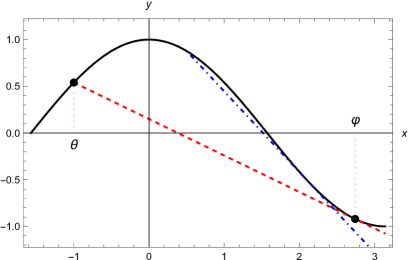
Figure 1: The black curve is $y=\cos x$. The red dashed and blue dash-dotted line segments are the ones corresponding to $\theta=-1.0$ and $0.5$, respectively. In particular, for $\theta=-1.0$, the line segment meets tangentially with the cosine curve at $\varphi\approx 2.74$. From this graph, it is evident that as $\theta$ increases from $-\pi$ to $\pi/2$, the corresponding $\varphi\in[\pi/2,\pi]$ as well as $\varphi-\theta$ decrease where as $\varphi+\theta$ increases. These observations are stated in Corollary 1 and proven in the Appendix.

Corollary 2.

Let $J$ be the interval $[-\pi/2,0]$. Then

$$\{\varphi(\theta)\colon\theta\in J\}\subset(\frac{\pi}{2},\pi),$$ (11a)

$$\{\varphi(\theta)-\theta\colon\theta\in J\}\subset(\frac{\pi}{2},\frac{3\pi}{2})$$ (11b)

and

$$\{\varphi(\theta)+\theta\colon\theta\in J\}\subset(0,\pi).$$ (11c)

Proof.

Eq. (11a) is a directly consequence of Eq. (8) in Lemma 1. Eqs. (11b) and (11c) follows from Corollary 1 and Eq. (11a). ∎

II.2 A New Proof Of The ML Bound And A New Expression Of $\boldsymbol{\alpha_{<}(\epsilon)}$

I use the following notations. Every time-independent Hamiltonian is formally written as $\sum_{j}E_{j}\ket{E_{j}}\bra{E_{j}}$ with $\ket{E_{j}}$’s being the normalized energy eigenstates of the Hamiltonian and $E_{0}$ being the ground state energy. Furthermore, a normalized initial pure state $\ket{\Psi(0)}$ is formally written as $\sum_{j}a_{j}\ket{E_{j}}$.

Theorem 1 (ML bound).

The evolution time $\tau$ needed for any quantum state to evolve to another state whose fidelity between them is $\epsilon$ under a time-independent Hamiltonian obeys

$$\frac{\tau}{\hbar}\geq\max_{\theta\in K_{\epsilon}}\frac{\cos\theta-\sqrt{\epsilon}}{\braket{E-E_{0}}\sin\varphi(\theta)}\equiv\frac{\pi\alpha_{<}(\epsilon)}{2\braket{E-E_{0}}},$$ (12)

where $K_{\epsilon}=[-\cos^{-1}(\sqrt{\epsilon}),0]$, $\varphi(\theta)$ is the unique root of Eq. (10) in the interval $[\max(\pi/2,|\theta|),\pi]$, and $\braket{E-E_{0}}$ is the expectation value of the energy of the system relative to the ground state energy of the Hamiltonian. (Note that denominator of the R.H.S. of Inequality (12) vanishes if the initial state is a ground state of the Hamiltonian. In this case, Inequality (12) still holds if one interprets its R.H.S. as $0$ if $\epsilon=1$ and $+\infty$ otherwise.) Last but not least, the $\theta$ maximizing the R.H.S. of Inequality (12) is unique.

Proof.

I only need to prove this theorem for pure initial states. If the initial state is mixed, then one just needs to consider the evolution of the purified state in the extended Hilbert space [4].

For any fixed $\theta\in(-\pi,\pi)$, using the notations stated at the beginning of this Subsection and by Corollary 1, I obtain

$$\sqrt{\epsilon} =\left|\braket{\Psi(0)}{\Psi(\tau)}\right|\geq\Re\left(\braket{\Psi(0)}{\Psi(\tau)}e^{iE_{0}\tau/\hbar}e^{-i\theta}\right)$$

$$=\sum_{j}|a_{j}|^{2}\cos\left[\frac{(E_{j}-E_{0})\tau}{\hbar}+\theta\right]$$

$$\geq\sum_{j}|a_{j}|^{2}\left[\cos\theta-\frac{(E_{j}-E_{0})\tau\sin\varphi(\theta)}{\hbar}\right]$$

$$=\cos\theta-\frac{\braket{E-E_{0}}\tau\sin\varphi(\theta)}{\hbar}.$$ (13)

Here $\Re(\cdot)$ denotes the real part of its argument. Therefore,

$$\frac{\tau}{\hbar}\geq\sup_{\theta\in(-\pi,\pi)}\frac{\cos\theta-\sqrt{\epsilon}}{\braket{E-E_{0}}\sin\varphi(\theta)}$$ (14)

provided that $\braket{E-E_{0}}>0$. If $\braket{E-E_{0}}=0$, $\ket{\Psi(0)}$ is a ground state of the Hamiltonian. In this case, Inequality (13) still holds according to the convention stated in this Theorem. Furthermore, $\braket{E-E_{0}}$ can never be negative.

From Eq. (11a) in Corollary 11, $\sin\varphi>0$. Thus, I may exclude those $\theta$’s with $\cos\theta-\sqrt{\epsilon}<0$ from the supremum calculation in the R.H.S. of Inequality (14). That is to say, I only need to consider those $\theta\in[-\cos^{-1}(\sqrt{\epsilon}),\cos^{-1}(\sqrt{\epsilon})]\subset[-\pi/2,\pi/2]$. In this domain, Corollary 1 demands $1/\sin\varphi$ to be a decreasing function of $\theta$. Combined with the fact that $\cos\theta-\sqrt{\epsilon}$ is an even function and that the R.H.S. of Inequality (14) is continuous for $\theta\in[-\cos^{-1}(\sqrt{\epsilon}),\cos^{-1}(\sqrt{\epsilon})]$, I conclude that the supremum in the R.H.S. of Inequality (14) can be replaced by maximum over $\theta\in K_{\epsilon}=[-\cos^{-1}(\sqrt{\epsilon}),0]$. Therefore, I obtain Inequality (12).

Recall from the proof of Corollary 1 that $\varphi$ is a differentiable function of $\theta$. From Eqs. (10) and (A.3),

$$\frac{d}{d\theta}\left(\frac{\cos\theta-\sqrt{\epsilon}}{\sin\varphi}\right)=0$$

$$\Longleftrightarrow{} (\cos\theta-\sqrt{\epsilon})(\sin\varphi-\sin\theta)=(\cos\varphi-\cos\theta)\sin\theta$$

$$\Longleftrightarrow{} \cos\frac{\varphi-\theta}{2}=\sqrt{\epsilon}\cos\frac{\varphi+\theta}{2}.$$ (15)

Since $\theta\in K_{\epsilon}\subset I_{1}$, Corollaries 1 and 11 demand that the L.H.S. and R.H.S. of the last line of Eq. (15) are increasing and decreasing functions of $\theta\in I_{1}$, respectively. Therefore, the $\theta\in K_{\epsilon}$ that maximizes the R.H.S. of Inequality (12) must be unique. ∎

Remark 2.

The expression of $\alpha_{<}(\epsilon)$ in the R.H.S. of Inequality (12) is equivalent to that of Eq. (4) originally obtained by Giovannetti et al. in Ref. [4]. In fact, they can be transformed from one to another via the equations $q=-\tan\theta$ and $\theta=\phi$ relating the optimized $\theta,\phi$ and $q$. Besides, Eq. (2) can be simplified as $m\cos\theta=\sin\varphi$. From its proof, it is straightforward to see that the ML bound in Theorem 1 can slightly strengthen to

$$\frac{\tau}{\hbar}\geq\max_{\theta\in K_{\epsilon}}\frac{\cos\theta-\sqrt{\epsilon}}{\braket{E-\underline{E}}\sin\varphi(\theta)}$$ (16)

where $\underline{E}=\operatorname{ess\ sup}\{E\colon\sum_{E_{j}<E}|a_{j}|^{2}=0\}$. In fact, Inequality (16) had been reported in Ref. [5].

II.3 $\boldsymbol{\alpha_{>}(\epsilon)=\alpha_{<}(\epsilon)}$

From now on, I denote the $\theta$ that maximizes the R.H.S. of Inequality (12) by $\theta_{\text{opt}}$. Moreover, I denote $\varphi(\theta_{\text{opt}})$ by $\varphi_{\text{opt}}$.

Theorem 2.

For each $\epsilon\in[0,1]$, there exists a pair of (pure) quantum state and time-independent Hamiltonian saturating the ML bound in Theorem 1. In fact, for $\epsilon=1$, any quantum state and Hamiltonian pair can saturate the ML bound. For $\epsilon\in[0,1)$, an initial (pure and normalized) quantum state $\ket{\Psi(0)}$ and a Hamiltonian pair saturate the ML bound if and only if

$$\ket{\Psi(0)}=a_{0}\ket{E_{0}}+a_{1}\ket{E_{1}}$$ (17)

with $E_{1}>E_{0}$, $(E_{1}-E_{0})\tau/\hbar=\varphi_{\text{opt}}-\theta_{\text{opt}}>0$ and

$$|a_{1}|^{2}=\frac{\sin\left|\theta_{\text{opt}}\right|}{2\sin\left(\frac{\varphi_{\text{opt}}-\theta_{\text{opt}}}{2}\right)\cos\left(\frac{\varphi_{\text{opt}}+\theta_{\text{opt}}}{2}\right)}.$$ (18)

(Note that here the required time-independent Hamiltonian $H$ appears implicitly via its energy eigenstates in Eq. (17). Explicitly, $H=E_{0}\ket{E_{0}}\bra{E_{0}}+E_{1}\ket{E_{1}}\bra{E_{1}}+H^{\prime}$ where $H^{\prime}\geq E_{0}$ is a time-independent Hamiltonian whose support equals the orthogonal complement of the span of $\ket{E_{0}}$ and $\ket{E_{1}}$. Note further that although $H^{\prime}$ does not affect the evolution of $\ket{\Psi(0)}$, the requirement $H^{\prime}\geq E_{0}$ is essential though technical. This is because $H^{\prime}$ makes the ML bound sub-optimal by shifting the ground state energy if it has an eigenvalue less than $E_{0}$.) Thus, $\alpha(\epsilon)=\alpha_{<}(\epsilon)$.

Proof.

For $\epsilon=1$, Inequality (12) becomes $\tau\geq 0$. Since $\epsilon=F(\ket{\Psi(0)},\ket{\Psi(0)})=1$, this inequality is just an equality for any initial state $\ket{\Psi(0)}$ under the action of any Hamiltonian.

In the remaining proof, $\epsilon$ is assumed to be in $[0,1)$. By Corollary 1 and the proof of Theorem 1, the necessary and sufficient conditions for a pair of quantum state $\ket{\Psi(0)}$ and time-independent Hamiltonian to saturate the ML bound in Inequality (12) are:

1. the $\theta$ in Inequality (13) is equal to $\theta_{\text{opt}}\in K_{\epsilon}$; and

2. this $\theta=\theta_{\text{opt}}$ together with $\ket{\Psi(0)}$ also turn the Inequality (13) into an equality.

Using $|z|=\max_{\theta\in{\mathbb{R}}}\Re(ze^{-i\theta})$ of all $z\in{\mathbb{C}}$, a trick first used in QSL research in Ref. [7], the first line of Inequality (13) becomes an equality if and only if

1. $\braket{\Psi(0)}{\Psi(\tau)}\neq 0$ and $\theta=\theta_{\text{opt}}=\arg(\braket{\Psi(0)}{\Psi(\tau)}$ $e^{iE_{0}\tau/\hbar})\bmod 2\pi$; or

2. $\braket{\Psi(0)}{\Psi(\tau)}=0$ and $\theta=\theta_{\text{opt}}$ can be any real number.

Note that $\tau>0$ as $\epsilon<1$. For each term in the second line of Inequality (13), I set $x=(E_{j}-E_{0})\tau/\hbar+\theta$ and apply Corollary 1 to it. In this way, I know that the third line of Inequality (13) becomes an equality if and only if $a_{j}=0$ whenever $E_{j}\geq E_{0}$ and $(E_{j}-E_{0})\tau/\hbar-\theta_{\text{opt}}\notin\{\theta_{\text{opt}},\varphi_{\text{opt}}\}$. In other words, the (normalized) initial state must be in the form of Eq. (17) with $E_{1}>E_{0}$ and $(E_{1}-E_{0})\tau/\hbar=\varphi_{\text{opt}}-\theta_{\text{opt}}>0$. To conclude, for a given $\epsilon\in[0,1)$, the initial state $\ket{\Psi(0)}$ saturating the ML bound are the ones given by Eq. (17) with $\theta_{\text{opt}}\in K_{\epsilon}\subset[-\pi/2,0]$. And the corresponding Hamiltonian is the one with $(E_{1}-E_{0})\tau/\hbar=\varphi_{\text{opt}}-\theta_{\text{opt}}$.

Recall that $\theta_{\text{opt}}$ must also equal the argument of $\braket{\Psi(0)}{\Psi(\tau)}e^{iE_{0}\tau/\hbar}\bmod 2\pi$ if $\braket{\Psi(0)}{\Psi(\tau)}\neq 0$. Thus, $a_{1}$ in Eq. (17) obeys

$$\tan\theta_{\text{opt}} =\frac{\Im\left(\braket{\Psi(0)}{\Psi(\tau)}e^{iE_{0}\tau/\hbar}\right)}{\Re\left(\braket{\Psi(0)}{\Psi(\tau)}e^{iE_{0}\tau/\hbar}\right)}$$

$$=\frac{-|a_{1}|^{2}\sin(\varphi_{\text{opt}}-\theta_{\text{opt}})}{|a_{0}|^{2}+|a_{1}|^{2}\cos(\varphi_{\text{opt}}-\theta_{\text{opt}})}$$

$$=\frac{-|a_{1}|^{2}\sin(\varphi_{\text{opt}}-\theta_{\text{opt}})}{1-|a_{1}|^{2}[1-\cos(\varphi_{\text{opt}}-\theta_{\text{opt}})]}$$ (19)

where $\Im(\cdot)$ is the imaginary part of its argument. By changing $|a_{1}|^{2}$ as the subject, I get

$$|a_{1}|^{2} =\frac{\tan\theta_{\text{opt}}}{\tan\theta_{\text{opt}}[1-\cos(\varphi_{\text{opt}}-\theta_{\text{opt}})]-\sin(\varphi_{\text{opt}}-\theta_{\text{opt}})}$$

$$=\frac{\sin\left|\theta_{\text{opt}}\right|}{2\sin\left(\frac{\varphi_{\text{opt}}-\theta_{\text{opt}}}{2}\right)\cos\left(\frac{\varphi_{\text{opt}}+\theta_{\text{opt}}}{2}\right)},$$ (20)

which is Eq. (18). Although Eq. (19) is ill-defined when its denominator is zero, Eq. (18) is well-defined and correct in all cases. Specifically, the first case for Eq. (19) to be ill-defined is that $\theta_{\text{opt}}=-\pi/2\bmod 2\pi$. Then, the vanishing denominator of Eq. (19) simplifies to $|a_{1}|^{2}=[2\sin^{2}(\varphi_{\text{opt}}/2+\pi/4)]^{-1}$. It is straightforward to check that this expression reduces to Eq. (18). The other case of concern is when $\sqrt{\epsilon}=\braket{\Psi(0)}{\Psi(\tau)}=0$. This case reduces to $\varphi_{\text{opt}}-\theta_{\text{opt}}=\pi$ and $|a_{1}|^{2}=1/2$ by Eq. (11b). And from Corollary 1, I know that $\cos\varphi_{\text{opt}}=\cos\theta_{\text{opt}}-\pi\sin\varphi_{\text{opt}}$. This gives $\tan\varphi_{\text{opt}}=\tan\theta_{\text{opt}}=-2/\pi$. Eliminating $\varphi_{\text{opt}}$ from Eq. (18) and using the fact that $\sin\theta_{\text{opt}}\neq 0$, I obtain $|a_{1}|^{2}=1/2$. This concludes that Eq. (18) is valid in all cases.

Finally, I need to check that $\ket{\Psi(0)}$ is a valid state by proving $|a_{1}|^{2}\in[0,1]$. Here I prove a slightly stronger result that $|a_{1}|^{2}\in[0,1/2]$. Eq. (18) implies that $|a_{1}|^{2}>0$. Furthermore, showing $|a_{1}|^{2}\leq 1/2$ is equivalent to proving

$$\quad-\sin\theta_{\text{opt}}=\sin\left|\theta_{\text{opt}}\right|\leq\sin\left(\frac{\varphi_{\text{opt}}-\theta_{\text{opt}}}{2}\right)\cos\left(\frac{\varphi_{\text{opt}}+\theta_{\text{opt}}}{2}\right)=\frac{1}{2}(\sin\varphi_{\text{opt}}-\sin\theta_{\text{opt}})$$

$$\Longleftrightarrow \quad\sin\varphi_{\text{opt}}+\sin\theta_{\text{opt}}=2\sin\left(\frac{\varphi_{\text{opt}}+\theta_{\text{opt}}}{2}\right)\cos\left(\frac{\varphi_{\text{opt}}-\theta_{\text{opt}}}{2}\right)\geq 0.$$ (21)

From Eqs. (11b) and (11c) in Corollary 11, I conclude that the last line of Inequality (21) is true. In other words, $\ket{\Psi(0)}$ is a valid normalized initial quantum state saturating the ML bound. This completes the proof. ∎

Remark 3.

Theorem 2 can be used to derive the following result reported in Ref. [5]. For any $\epsilon\in[0,1]$ and any initial normalized pure state $\ket{\Psi(0)}$, there is a time-independent Hamiltonian $H$ acting on a Hilbert space of dimension at least 2 such that $|\braket{\Psi(0)}{\Psi(\tau)}|^{2}=\epsilon$ with $\tau$ saturating the ML bound. Likewise, for any $\epsilon\in[0,1]$ and any time-independent Hamiltonian $H$ that is not proportional to the identity operator, there is a normalized initial state $\ket{\Psi(0)}$ such that $|\braket{\Psi(0)}{\Psi(\tau)}|^{2}=\epsilon$ with $\tau$ saturating the ML bound. The proof is simple. As the two settings are trivially true for $\epsilon=1$, I only need to consider the case of $\epsilon\in[0,1)$. For the first setting, once $\epsilon$ is given, $\theta_{\text{opt}}$ is fixed. One chooses $\tau=1$ and picks $E_{0}$ and $E_{1}$ satisfying the constraints in Theorem 2. Moreover, one selects an arbitrary but fixed normalized state $\ket{\Phi}$ orthogonal to $\ket{\Psi(0)}$. Let $\ket{E_{0}}=a_{0}\ket{\Psi(0)}+a_{1}\ket{\Phi}$ and $\ket{E_{1}}=a_{1}\ket{\Psi(0)}-a_{0}\ket{\Phi}$, where $a_{j}$’s are non-negative real numbers with $a_{1}$ obeying Eq. (18). Then, it is easy to check that $\ket{\Phi(0)}$ satisfies Eq. (17) and $H=E_{0}\ket{E_{0}}\bra{E_{0}}+E_{1}\ket{E_{1}}\bra{E_{1}}$ is the required time-independent Hamiltonian. For the second setting, since $H$ is not proportional to the identity operator, it has at least two distinct eigenenergies, say the ground state energy $E_{0}$ and an excited state energy $E_{1}$. Surely, for any fixed $\epsilon\in[0,1)$, one can find $\tau$ making $E_{0},E_{1}$ to satisfy the constraints in Theorem 2. Clearly, the normalized state in the form of Eq. (17) with probability amplitude $a_{1}$ satisfying Eq. (18) is the required initial pure quantum state.

Corollary 3.

$\alpha_{>}(\epsilon)=\alpha_{<}(\epsilon)$ where

$$\alpha_{>}(\epsilon) =\min_{|a_{1}|^{2}\in[\frac{1-\sqrt{\epsilon}}{2},\frac{1}{2}]}\frac{4|a_{1}|^{2}}{\pi}\sin^{-1}\sqrt{\frac{1-\epsilon}{4|a_{1}|^{2}\left(1-|a_{1}|^{2}\right)}}$$

$$=\min_{\mu\in[\sin^{-1}\sqrt{1-\epsilon},\frac{\pi}{2}]}\frac{2\mu\left[1-\sqrt{1-(1-\epsilon)\csc^{2}\mu}\right]}{\pi}.$$ (22)

Here $|a_{1}|^{2}$ and $\mu$ are related by

$$\mu=\sin^{-1}\sqrt{\frac{1-\epsilon}{4|a_{1}|^{2}\left(1-|a_{1}|^{2}\right)}}.$$ (23)

Proof.

The proof of Theorem 2 clearly shows that a state $\ket{\Psi(0)}$ saturating the ML bound must be in the form of Eq. (17). Besides, the optimality condition depends on the magnitude rather than the phase of $a_{1}$. Since for a given $\epsilon\in[0,1]$, the values of the optimal $\theta=\theta_{\text{opt}}$ and the corresponding $\varphi=\varphi_{\text{opt}}$ are fixed. So from Eq. (18), for a given $\epsilon\in[0,1]$, there is only one $|a_{1}|^{2}\in[0,1/2]$ that makes the state $\ket{\Psi(0)}$ saturating the ML bound. As

$$\epsilon =\left|\braket{\Psi(0)}{\Psi(\tau)}\right|^{2}$$

$$=1-4|a_{1}|^{2}\left(1-|a_{1}|^{2}\right)\sin^{2}\left[\frac{(E_{1}-E_{0})\tau}{2\hbar}\right],$$ (24)

I conclude that

$$\frac{\tau}{\hbar}=\min_{|a_{1}|^{2}\in[0,1/2]}\frac{2}{E_{1}-E_{0}}\sin^{-1}\sqrt{\frac{1-\epsilon}{4|a_{1}|^{2}\left(1-|a_{1}|^{2}\right)}}$$ (25)

as long as $1-\epsilon\leq 4|a_{1}|^{2}(1-|a_{1}|^{2})$ or equivalently $(1-\sqrt{\epsilon})/2\leq|a_{1}|^{2}\leq(1+\sqrt{\epsilon})/2$. Note that if $1-\epsilon>4|a_{1}|^{2}(1-|a_{1}|^{2})$, Eq. (24) has no real-valued solution for $\tau$. Therefore, the corresponding value of $|a_{1}|^{2}$ can be excluded from the $\alpha_{>}(\epsilon)$ calculation. Since $\braket{E-E_{0}}=|a_{1}|^{2}E_{1}$ for $\ket{\Psi(0)}$, I prove the validity of the first equality in Eq. (22).

Since Eq. (23) is a bijection from $|a_{1}|^{2}\in[(1-\sqrt{\epsilon})/2,1/2]$ to $\mu\in[\sin^{-1}\sqrt{1-\epsilon},\pi/2]$ whenever $\epsilon<1$, the last equality in Eq. (22) is correct if $\epsilon\in[0,1)$. Finally, $\alpha_{>}(0)=0$ according to the last line of Eq. (22). So, Eq. (22) is also true when $\epsilon=1$. ∎

Remark 4.

Actually, the first line of Eq. (22) is equal to the expression of $\alpha_{>}(\epsilon)$ originally reported in Ref. [4] and reproduced as Eq. (5) in this paper. To show this fact, I let $z=|a_{1}|^{2}$. Then, my claim is correct if

$$2\sin^{-1}\sqrt{\frac{1-\epsilon}{4z(1-z)}}=\cos^{-1}\left[1-\frac{1-\epsilon}{2z(1-z)}\right].$$ (26)

Note that the values of arc sine and arc cosine in Eq. (26) are in the principle branch. So the correctness of Eq. (26) can be proven by taking cosine in both sides of this equation and then by using compound angle formula. Nevertheless, there is a slight difference in the region of minimization. In Corollary 23, $|a_{1}|^{2}$ is minimized over a smaller interval of $[(1-\sqrt{\epsilon})/2,1/2]$, whereas in Ref. [4], it is minimized over a larger interval of $[0,1]$.

III Efficient And Reliable Computation Of $\boldsymbol{\alpha(\epsilon)}$

One could compute $\alpha(\epsilon)$ through $\alpha_{<}(\epsilon)$ in Eq. (12). This method involves two maximizations — one for finding $\varphi$ given $\theta$ and the other for maximizing $(\cos\theta-\sqrt{\epsilon})/\sin\varphi$ over $\theta$. Hence, it is very slow if generic optimization methods are used. (There is a minor point. For the trivial case of $\epsilon=1$, there is nothing to maximize in Eq. (12) as $\theta$ is fixed and value of $\varphi$ no longer relevant even if one insists on computing $\alpha(0)$ numerically. I exclude this special case in almost all the subsequent discussions.) Another method is to compute the above two maximizations by finding the unique roots of $f_{\theta}(\varphi)=0$ and the last line of Eq. (15), respectively. This is faster. Nevertheless, I do not discuss the rate of convergence and stability of this approach here because I am going to report a much better method in the next paragraph. The third way is to compute $\alpha(\epsilon)$ via $\alpha_{>}(\epsilon)$ in Eq. (22) using a general minimization algorithm. This is faster than the first method as it involves only one minimization over $|a_{1}|^{2}$ or $\mu$ though it is slower than the second method. (Actually, no minimization is required for the special case of $\epsilon=0$ as the interval for minimization becomes a point.) Minimization via $\mu$ is preferred as it is numerically more stable. The only potential trouble is the serious rounding error in computing the square root part of the expression in the R.H.S. of Eq. (22) when $\mu\approx\sin^{-1}\sqrt{1-\epsilon}$ or $\pi/2$. Fortunately, this lost of significance has very little effect on the accuracy of the whole expression to be minimized in the second line of Eq. (22).

There is one more way to compute $\alpha(\epsilon)$ that could be more efficient than a general minimization algorithm that is applicable to a smooth target function with possibly multiple local minima. The trick is to use an additional property of the function to be minimized. From the proofs of Theorem 2 and Corollary 23 together with the fact that Eq. (23) is a diffeomorphism if $\epsilon\in[0,1]$, there is a unique $\mu\in[\sin^{-1}\sqrt{1-\epsilon},\pi/2]$ minimizing the second line of Eq. (22) if $\epsilon\in[0,1)$. By differentiating the expression in the second line of Eq. (22), I find that this minimizing $\mu$ obeys

$$g(\mu)\equiv\frac{1+(1-\epsilon)(\mu\cot\mu-1)\csc^{2}\mu}{\sqrt{1-(1-\epsilon)\csc^{2}\mu}}-1=0.$$ (27)

(For $\epsilon=1$, Eq. (27) is trivial, giving no constraint on $\mu$. Nevertheless, substituting any real-valued $\mu$ to Eq. (22) still gives the correct answer of $\alpha_{>}(0)=0$ if one insists on computing it numerically. For $\epsilon=0$, no minimization is needed as $\mu$ must be $\pi/2$.) In this way, this particular minimization problem is reduced to a potentially much easier problem of finding a unique simple root in a closed interval of a single equation. (In contrast, the second method requires root finding of two coupled equations for Eq. (15) depends on the solution of $f_{\theta}(\varphi)=0$.) Numerical experiment shows that Newton’s method converges for any input $\epsilon\in(0,1)$ using the initial guess $(\sin^{-1}\sqrt{1-\epsilon}+\pi/2)/2$, namely, the mid-point of the possible interval for $\mu$. The plot of $g(\mu)$ in Fig. 2 for various $\epsilon$ strongly suggests that the basin of attraction of Newton’s method is the whole possible interval for $\mu$. In addition, rounding and truncation errors are not significant in evaluating $g(\mu)$ as well as the R.H.S. of Eq. (22). Consequently, one can accurately find the simple root $\mu\in[\sin^{-1}\sqrt{1-\epsilon},\pi/2]$ in Eq. (27) through the quadratically convergent Newton’s method. Substituting this root to Eq. (22) gives $\alpha(\epsilon)$. Among the four, this is the fastest method to compute $\alpha(\epsilon)$ for $\epsilon\neq 1$. Surely, one may further speed things up by accelerated convergence methods, but this is not the main point here.

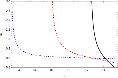
Figure 2: The function $g(\mu)$ for $\epsilon=0.1$ (black solid curve), $0.5$ (red dashed curve) and $0.9$ (blue dot-dashed curve). It is clear from the shape of these curves and their zeros that Newton’s method converges for almost any initial guess of $\mu\in[\sin^{-1}\sqrt{1-\epsilon},\pi/2]$.

Evaluating $\alpha_{>}(\epsilon)$ through numerically finding root of Eq. (6) implicitly suggested in Ref. [4], in contrast, can be problematic. It is not clear if Eq. (6) has a unique root in the interval of interest although plotting the graph of Eq. (6) strongly suggests it is indeed the case. A more serious problem is numerical instability. Observe that the R.H.S. of Eq. (6) diverges at $z=(1-\sqrt{\epsilon})/2$. Furthermore, numerical computation shows that the root of Eq. (6) approaches $(1-\sqrt{\epsilon})/2$ as $\epsilon\to 1^{-}$. In other words, when $\epsilon$ is close to $1$, one has to determine the precise location of the root of Eq. (6) close to a singular point. To make things worse, the slope of the R.H.S. of Eq. (5) diverges at $z=(1-\sqrt{\epsilon})/2$. Hence, a highly accurate root $z$ of Eq. (6) is required to evaluate $\alpha_{>}(\epsilon)$ via Eq. (5). All these can only be done with great care. No wonder why the values of $\alpha_{>}(\epsilon)$ computed in this way using Newton’s, secant and Brent’s methods are either inaccurate or divergent when $\epsilon\lesssim 1$. For example, using the initial guess $p(1-\sqrt{\epsilon}/2+(1-p)/2$ with $p=1/2$, Newton’s method fails to find the root when $\epsilon\gtrsim 0.76$. Increasing $p$ to $0.99$, Newton’s method works for $\epsilon=0.76$ but fails to find the root accurately for $\epsilon\gtrsim 0.9$. Depending on the value of $\epsilon$, great care in choosing initial guess, bounding interval and stopping criterion are needed to obtain the root of Eq. (6) and hence the value of $\alpha_{>}(\epsilon)$ correctly and accurately. These complications make numerically evaluating $\alpha_{>}(\epsilon)$ by solving Eq. (6) unattractive.

Appendix A Appendix

Proof of Lemma 1.

Obviously, Inequality (7) follows directly from the first line of Eq. (8). So I need to show that the supremum in the first line of Eq. (8) exists and is equal to the second line of the same equation. I first consider the case of $\theta\in(-\pi,\pi/2)$. Denote the slope of the line joining the points $(\theta,\cos\theta)$ and $(x,\cos x)$ on the cosine curve $y=\cos x$ by $M_{\theta}(x)=(\cos x-\cos\theta)/(x-\theta)$ if $x\neq\theta$ and $M_{\theta}(\theta)=-\sin\theta$ if $x=\theta$. Clearly, $M_{\theta}(x)>0$ if $x>\theta$ and $\cos x>\cos\theta$. Moreover, for any fixed $b\in[-1,\cos\theta)$, the set $S_{b,\theta}=\{x>\theta\colon\cos x=b\}$ is non-empty and $\min S_{b,\theta}\in[|\theta|,\pi]$. Besides, $M_{\theta}(x)<M_{\theta}(y)<0$ whenever $x,y\in S_{b,\theta}$ and $x<y$. As a result,

$$A_{\theta} =-\inf_{x>\theta}M_{\theta}(x)=-\inf_{b\in[-1,\cos\theta)}M_{\theta}(\min S_{b,\theta})$$

$$=-\min_{x\in[|\theta,\pi]}M_{\theta}(x),$$ (A.1)

where the last line is due to continuity of $M_{\theta}(x)$ and the fact that the closure of $\{\min S_{b,\theta}\colon b\in[-1,\cos\theta)\}$ is $[|\theta|,\pi]$. Therefore, $A_{\theta}$ is well-defined and the second line of Eq. (8) is correct when $\theta\in(-\pi,-\pi/2]$.

For the case of $\theta\in(-\pi/2,\pi/2)$. Note that $y=\cos x$ is strictly concave in the domain $x\in(-\pi/2,\pi/2)$. So, Jensen’s inequality demands that

$$p\cos\theta+(1-p)\cos\frac{\pi}{2}<\cos\left[p\theta+\frac{(1-p)\pi}{2}\right]$$ (A.2)

for $p=(\pi/2-x)/(\pi/2-\theta)$ as long as $-\pi/2<\theta<x<\pi/2$. Simplifying Eq. (A.2) gives $M_{\theta}(x)>M_{\theta}(\pi/2)$. Therefore, $\min_{x\in[|\theta|,\pi]}M_{\theta}(x)=\min_{x\in[\pi/2,\pi]}M_{\theta}(x)$ if $|\theta|<\pi/2$. So, $A_{\phi}$ is well-defined and Eq. (8) is valid when $\theta\in(-\pi/2,\pi/2)$.

For the case of $\theta\in[\pi/2,\pi)$, $M_{\theta}(x)>M_{\theta}(\theta)$ for all $x\in(\theta,\pi]$ due to strict convexity of $y=\cos x$ in this interval. Thus, $A_{\theta}=-\lim_{x\to\theta^{+}}M_{\theta}(x)=\sin\theta$. In other words, Eq. (8) holds if $\pi/2\leq\theta<\pi$.

Finally, I show that the supremum (and hence maximum when $-\pi<\theta<\pi/2$) in Eq. (8) is attained by a unique $x\in[\max(\pi/2,|\theta|),\pi]$. Suppose there were another such $y\neq x$ in the same domain that maximizes the second line of Eq. (8). Then the straight line passing through $(\theta,\cos\theta)$, $(x,\cos x)$ must also pass through $(y,\cos y)$. Since the cosine function is strictly convexity in the interval $(\pi/2,\pi]$, Jensen’s inequality implies that $\cos x+\cos y>2\cos([x+y]/2)$. Hence, $M_{\theta}([x+y]/2)<M_{\theta}(x)$, contradicting the assumption that $x$ maximizes Eq. (8). This completes the proof. ∎

Proof of Corollary 1.

Consider the case of $\theta\in I_{1}$. Since the maximum in the second line of Eq. (8) is attained at $x=\varphi$, the line $L$ passing through $(\theta,\cos\theta)$ and $(\varphi,\cos\varphi)$ must be a tangent to the cosine curve $y=\cos x$ at $x=\varphi$. For the case of $\theta\in I_{2}$, it is clear that the line $L$ and the cosine curve meet tangentially at $x=\varphi=\theta$. Therefore in all cases, $-A_{\theta}$ equals the slope of the cosine curve at $x=\varphi$, namely, $-\sin\varphi$. Consequently, Inequality (7) can be rewritten as Inequality (9). Besides, $f_{\theta}(x)\geq 0$ for all $x\geq\theta$.

Suppose $\theta\in I_{1}$. Then the smooth function $f_{\theta}(x)$ has exactly three roots in $[\theta,\pi]$ counted by multiplicity, namely, a simple root at $x=\theta$ and a double root at $x=\varphi$. For otherwise, $f_{\theta}(x)$ has at least four roots in $[\theta,\pi]$. Hence, $f_{\theta}^{\prime}(x)=-\sin x+\sin\varphi$ has at least three roots in $(\theta,\pi)\subset(-\pi,\pi)$, which is absurd. Furthermore, using the notation and proof of Lemma 1, $M_{\theta}(x)>M_{\theta}(\varphi)$ for all $x>\pi$. This implies $f_{\theta}(x)>0$ whenever $x>\pi$. Therefore, $\theta$ and $\varphi$ are the only roots of $f_{\theta}(x)$ in the domain $[\theta,+\infty)$. In other words, $x=\varphi$ is the unique point in $(\theta,+\infty)$ that maximizes $(\cos\theta-\cos x)/(x-\theta)$. Besides, $x\in[\max(\pi/2,|\theta|),\pi]$. The case when $\theta\in I_{2}$ can be proven in the same manner.

From Lemma 1, $\varphi=\theta$ whenever $\theta\in I_{2}$. Hence, $\varphi$, $\varphi-\theta$ and $\varphi+\theta$ are increasing, decreasing and increasing functions of $\theta\in I_{2}$, respectively.

I now show that $\varphi$ and $\varphi-\theta$ are decreasing functions of $\theta\in I_{1}$. As already shown in the second paragraph of this proof, for each $\theta\in I_{1}$, $f_{\theta}(\varphi)=0$ has a unique solution $\varphi\in I_{2}$. Moreover, this $\varphi$ is equal to the $x$ that maximizes the second line of Eq. (8) in Lemma 1. Regarding $f_{\theta}(\varphi)$ as a function of $\theta$ and $\varphi$, then the implicit function theorem implies that

$$\frac{d\varphi}{d\theta}=\frac{\sin\varphi-\sin\theta}{(\varphi-\theta)\cos\varphi}$$ (A.3)

provided that the denominator of Eq. (A.3), namely, $\partial f_{\theta}/\partial\varphi$, is non-zero. This condition is satisfied as $\theta\in I_{1}$ and $\varphi\in I_{2}$. Consequently, from Eq. (A.3), to prove that $\varphi$ and hence $\varphi-\theta$ are decreasing functions of $\theta\in I_{1}$, I have to show that $\sin\varphi\geq\sin\theta$ for $\theta\in I_{1}$. Since this inequality is trivially true when $-\pi/2\leq\theta\leq 0$, I only need to consider the remaining case of $\theta\in(0,\pi/2)$. In this case, it suffices to prove that $\varphi\leq\pi-\theta$. It is straightforward to see that the line joining $(\theta,\cos\theta)$ and $(\pi-\theta,\cos[\pi-\theta])$ meets the cosine curve $y=\cos x$ also at $x=\pi/2$. Furthermore, convexity of this cosine curve in the domain $[\pi/2,\pi]$ implies that this cosine curve must lie below this line for $x\in(\pi/2,\pi-\theta)$. Hence, the unique maximum point in the second line of Eq. (8) is attained at $x=\varphi<\pi-\theta$. So, it is proved.

Finally, I show that $\varphi+\theta$ is an increasing function of $\theta\in I_{1}$. I claim that $d\varphi/d\theta\geq-1$ for $\theta\in I_{1}$. From Eq. (A.3) and the fact that $\varphi\in I_{2}$, I obtain

$$\quad\frac{d\varphi}{d\theta}\geq-1$$

$$\Longleftrightarrow \quad\sin\varphi(\sin\varphi-\sin\theta)\leq-(\varphi-\theta)\sin\varphi\cos\varphi$$

$$\Longleftrightarrow \quad\sin\varphi(\sin\varphi-\sin\theta)\leq\cos\varphi(\cos\varphi-\cos\theta)$$

$$\Longleftrightarrow \quad\sin\left(\frac{3\varphi+\theta}{2}\right)\sin\left(\frac{\varphi-\theta}{2}\right)\geq 0.$$ (A.4)

Since $\varphi-\theta$ is a decreasing function of $\theta$ in the domain $I_{1}$, $0<\varphi-\theta<2\pi$ in the same domain. Therefore, it suffices to prove that $0\leq 3\varphi+\theta\leq 2\pi$ for $\theta\in I_{1}$. As $\theta>-\pi$ and $\varphi>\pi/2$, surely $3\varphi+\theta>0$. Note that $3\varphi+\theta=4\varphi-(\varphi-\theta)$ is a difference of a decreasing and an increasing function of $\theta\in I_{1}$. As a result, $3\varphi+\theta<\left.(3\varphi+\theta)\right|_{\theta=\pi/2}=2\pi$. This completes the proof. ∎

References

- Margolus and Levitin [1996] N. Margolus and L. B. Levitin, in Proceedings of the 4th workshop on physics and computation (PHYSCOMP 96), edited by T. Toffoli, M. Biafore, and J. Leaõ (New England Complex Systems Institute, Cambridge, MA, 1996) p. 208.
- Margolus and Levitin [1998] N. Margolus and L. B. Levitin, Physica D 120, 188 (1998).
- Frey [2016] M. R. Frey, Quant. Inform. Proc. 15, 3919 (2016).
- Giovannetti et al. [2003] V. Giovannetti, S. Lloyd, and L. Maccone, Phys. Rev. A 67, 052109 (2003).
- Hörnedal and Sönnerborn [2023] N. Hörnedal and O. Sönnerborn, The Margolus-Levitin quantum speed limit for an arbitrary fidelity, arXiv:2301.10063v2 (2023).
- Chau [2010] H. F. Chau, Phys. Rev. A 81, 062133 (2010).
- Uhlmann [1992] A. Uhlmann, Phys. Lett. A 161, 329 (1992).