Scale-Adaptive Balancing of Exploration and Exploitation in Classical Planning

Abstract

Balancing exploration and exploitation has been an important problem in both adversarial games and automated planning. While it has been extensively analyzed in the Multi-Armed Bandit (MAB) literature, and the game community has achieved great success with MAB-based Monte Carlo Tree Search (MCTS) methods, the symbolic planning community has struggled to advance in this area. We describe how Upper Confidence Bound 1’s (UCB1’s) assumption of reward distributions with known bounded support shared among siblings (arms) is violated when MCTS/Trial-based Heuristic Tree Search (THTS) in previous work uses heuristic values of search nodes in classical planning problems as rewards. To address this issue, we propose a new Gaussian bandit, UCB1-Normal2, and analyze its regret bound. It is variance-aware like UCB1-Normal and UCB-V, but has a distinct advantage: it neither shares UCB-V’s assumption of known bounded support nor relies on UCB1-Normal’s unfounded conjectures on Student’s $t$ and $\chi^{2}$ distributions. Our theoretical analysis predicts that UCB1-Normal2 will perform well when the estimated variance is accurate, which can be expected in deterministic, discrete, finite state-space search, as in classical planning. Our empirical evaluation confirms that MCTS combined with UCB1-Normal2 outperforms Greedy Best First Search (traditional baseline) as well as MCTS with other bandits.

1 Introduction

From the early history of AI and in particular of automated planning and scheduling, heuristic forward search has been a primary methodology for tacking challenging combinatorial problems. A rich variety of search algorithms have been proposed, including Dijkstra search (Dijkstra 1959), A^∗/ WA^∗ (Hart, Nilsson, and Raphael 1968), and Greedy Best First Search (Bonet and Geffner 2001, GBFS). They are divided into three categories: optimizing, which must guarantee the optimality of the output, satisficing, which may or may not attempt to minimize solution cost, and agile, which ignores solution cost and focuses on finding a solution quickly. This paper focuses on the agile setting.

Unlike optimizing search, theoretical understanding of satisficing and agile search has been limited. Recent theoretical work on GBFS (Heusner, Keller, and Helmert 2017, 2018b, 2018a; Kuroiwa and Beck 2022) refined the concept of search progress in agile search, but only based on a post hoc analysis that depends on oracular information, making their insights difficult to apply to practical search algorithm design, although it has been recently applied to a learning-based approach (Ferber et al. 2022a). More importantly, their analysis is incompatible with a wider range of randomized algorithms (Nakhost and Müller 2009; Imai and Kishimoto 2011; Kishimoto, Zhou, and Imai 2012; Valenzano et al. 2014; Xie, Nakhost, and Müller 2012; Xie, Müller, and Holte 2014; Xie et al. 2014; Xie, Müller, and Holte 2015; Asai and Fukunaga 2017; Kuroiwa and Beck 2022) that outperform the deterministic baseline with randomized explorations; as a result, their detailed theoretical properties are largely unknown except for probabilistic completeness (Valenzano et al. 2014). It is unsurprising that analyzing randomized algorithms requires a statistical perspective, which is also growing more important due to recent advances in learned heuristic functions (Toyer et al. 2018; Ferber, Helmert, and Hoffmann 2020; Shen, Trevizan, and Thiébaux 2020; Ferber et al. 2022b; Rivlin, Hazan, and Karpas 2019; Gehring et al. 2022; Garrett, Kaelbling, and Lozano-Pérez 2016).

In this paper, we tackle the problem of balancing exploration and exploitation in classical planning through a statistical lens and from the perspective of MABs. Previous work showed that traditional forward search algorithms (A*, GBFS) can be seen as a form of MCTS, but we refine and recast this paradigm as a repeated process of collecting a reward dataset and exploring the environment based on estimates obtained from this dataset. This perspective reveals a theoretical issue in THTS (Schulte and Keller 2014), a MCTS modified for classical planning that uses UCB1: the optimization objective of classical planning has no a priori known bound, and this violates the bounded reward assumption of UCB1.

To apply MAB to classical planning without THTS’s theoretical issues, we propose UCB1-Normal2, a new Gaussian bandit, and GreedyUCT-Normal2, a new agile planning algorithm that combines MCTS with UCB1-Normal2, and show that GreedyUCT-Normal2 outperforms traditional agile algorithms (GBFS), existing MCTS-based algorithms (GreedyUCT, GreedyUCT*), and other MCTS-based algorithms combined with existing variance-aware bandits (UCB1-Normal and UCB-V).

In summary, our core contributions are as follows.

• We identify theoretical issues that arise when applying UCB1 to planning tasks.

• To address these issues, we present UCB1-Normal2, a new Gaussian bandit. We analyze its regret bound, which improves as the estimated variance is closer to the true variance, and is constant when they match. This makes it particularly powerful in a deterministic and finite state space such as classical planning.

• We present GreedyUCT-Normal2, a new forward search algorithm that combines UCB1-Normal2 with MCTS and outperforms existing algorithms in agile classical planning.

2 Background

2.1 Classical Planning

We define a propositional STRIPS Planning problem as a 4-tuple ${\left[P,A,I,G\right]}$ where $P$ is a set of propositional variables, $A$ is a set of actions, $I\subseteq P$ is the initial state, and $G\subseteq P$ is a goal condition. Each action $a\in A$ is a 4-tuple ${\left[\textsc{pre}(a),\textsc{add}(a),\textsc{del}(a),\textsc{c}(a)\right]}$ where $\textsc{c}(a)\in{\mathbb{Z}}^{0+}$ is a cost, $\textsc{pre}(a)\subseteq P$ is a precondition and $\textsc{add}(a),\textsc{del}(a)\subseteq P$ are the add-effects and delete-effects. A state $s\subseteq P$ is a set of true propositions (all of $P\setminus s$ is false), an action $a$ is applicable when $s\supseteq\textsc{pre}(a)$ (read: $s$ satisfies $\textsc{pre}(a)$), and applying action $a$ to $s$ yields a new successor state $a(s)=(s\setminus\textsc{del}(a))\cup\textsc{add}(a)$.

The task of classical planning is to find a sequence of actions called a plan $(a_{1},\cdots,a_{n})$ where, for $1\leq t\leq n$, $s_{0}=I$, $s_{t}\supseteq\textsc{pre}(a_{t+1})$, $s_{t+1}=a_{t+1}(s_{t})$, and $s_{n}\supseteq G$. A plan is optimal if there is no plan with lower cost $\sum_{t}\textsc{c}(a_{t})$. A plan is otherwise called satisficing. In this paper, we assume unit-cost: $\forall a\in A;\textsc{c}(a)=1$.

A domain-independent heuristic function $h$ in classical planning is a function of a state $s$ and the problem ${\left[P,A,I,G\right]}$, but the notation $h(s)$ usually omits the latter. It returns an estimate of the cumulative cost from $s$ to one of the goal states (which satisfy $G$), typically through a symbolic, non-statistical means including problem relaxation and abstraction. Notable state-of-the-art functions that appear in this paper include $h^{\mathrm{FF}},h^{\mathrm{max}},h^{\mathrm{add}}$, and $h^{\mathrm{GC}}$ (Hoffmann and Nebel 2001; Bonet and Geffner 2001; Fikes, Hart, and Nilsson 1972). Their implementation details are beyond the scope of this paper, and are included in the appendix Sec. LABEL:sec:heuristics.

2.2 Multi-Armed Bandit (MAB)

MAB (Thompson 1933; Robbins 1952; Bush and Mosteller 1953) is a problem of finding the best strategy to choose from multiple unknown reward distributions. It is typically depicted by a row of $K$ slot machines each with a lever or “arm.” Each time the player plays one of the machines and pulls an arm (a trial), the player receives a reward sampled from the distribution assigned to that arm. Through multiple trials, the player discovers the arms’ distributions and selects arms to maximize the reward.

The most common optimization objective of MAB is Cumulative Regret (CR) minimization. Let ${\textnormal{r}}_{i}$ ($1\leq i\leq K$) be a random variable (RV) for the reward that we would receive when we pull arm $i$. We call $p({\textnormal{r}}_{i})$ an unknown reward distribution of $i$. Let ${\textnormal{t}}_{i}$ be a RV of the number of trials performed on arm $i$ and $T=\sum_{i}{\textnormal{t}}_{i}$ be the total number of trials across all arms.

Definition 1.

The cumulative regret $\Delta$ is the gap between the optimal and the actual expected cumulative reward: $\textstyle\Delta=T\max_{i}{\mathbb{E}}[{\textnormal{r}}_{i}]-\sum_{i}{\mathbb{E}}[{\textnormal{t}}_{i}]{\mathbb{E}}[{\textnormal{r}}_{i}].$

Algorithms whose regret per trial $\Delta/T$ converges to 0 with $T\rightarrow\infty$ are called zero-regret. Those with a logarithmically upper-bounded regret, $O(\log T)$, are also called asymptotically optimal because this is the theoretical optimum achievable by any algorithm (Lai, Robbins et al. 1985).

Upper Confidence Bound 1 (Auer, Cesa-Bianchi, and Fischer 2002, UCB1) is a logarithmic CR MAB for rewards ${\textnormal{r}}_{i}\in[0,c]$ with known $c$. Let $r_{i1}\ldots r_{it_{i}}\sim p({\textnormal{r}}_{i})$ be $t_{i}$ i.i.d. samples obtained from arm $i$. Let $\hat{\mu}_{i}=\frac{1}{t_{i}}\sum_{j=1}^{t_{i}}r_{ij}$. To minimize CR, UCB1 selects $i$ with the largest Upper Confidence Bound defined below.

$$\begin{split}\text{UCB1}_{i}&\textstyle={\hat{\mu}_{i}+c\sqrt{{2\log T}/{t_{i}}}}\\ \text{LCB1}_{i}&\textstyle={\hat{\mu}_{i}-c\sqrt{{2\log T}/{t_{i}}}}\end{split}$$ (1)

For reward (cost) minimization, LCB1 instead select $i$ with the smallest Lower Confidence Bound defined above (e.g., in Kishimoto et al. (2022)), but we may use the terms U/LCB1 interchangeably. UCB1’s second term is often called an exploration term. Generally, an LCB is obtained by flipping the sign of the exploration term in a UCB. U/LCB1 refers to a specific algorithm while U/LCB refers to general confidence bounds. $c$ is sometimes set heuristically as a hyperparameter called the exploration rate.

2.3 Forward Heuristic Best-First Search

Classical planning problems are typically solved as a path finding problem defined over a state space graph induced by the transition rules, and the current dominant approach is based on forward search. Forward search maintains a set of search nodes called an open list. They repeatedly (1) (selection) select a node from the open list, (2) (expansion) generate its successor nodes, (3) (evaluation) evaluate the successor nodes, and (4) (queueing) reinsert them into the open list. Termination typically occurs when a node is expanded that satisfies a goal condition, but a satisficing/agile algorithm can perform early goal detection, which immediately checks whether any successor node generated in step (2) satisfies the goal condition. Since this paper focuses on agile search, we use early goal detection for all algorithms.

Within forward search, forward best-first search defines a particular ordering in the open list by defining node evaluation criteria (NEC) $f$ for selecting the best node in each iteration. Let us denote a node by $n$ and the state represented by $n$ as $s_{n}$. As NEC, Dijkstra search uses $f_{\mathrm{Dijkstra}}(n)=g(n)$ ($g$-value), the minimum cost from the initial state $I$ to the state $s_{n}$ found so far. A^∗ uses $f_{{A^{*}}}(n)=g(n)+h(s_{n})$, the sum of $g$-value and the value returned by a heuristic function $h$ ($h$-value). GBFS uses $f_{{\mathrm{GBFS}}}(n)=h(s_{n})$. Forward best-first search that uses $h$ is called forward heuristic best-first search. Dijkstra search is a special case of A^∗ with $h(s)=0$.

Typically, an open list is implemented as a priority queue ordered by NEC. Since the NEC can be stateful, e.g., $g(s_{n})$ can update its value, a priority queue-based open list assumes monotonic updates to the NEC because it has an unfavorable time complexity for removals. A^∗, Dijkstra, and GBFS satisfy this condition because $g(n)$ decreases monotonically and $h(s_{n})$ is constant.

MCTS is a class of forward heuristic best-first search that represents the open list as the leaves of a tree. We call the tree a tree-based open list. Our MCTS is based on the description in Keller and Helmert (2013) and Schulte and Keller (2014), whose implementation details are available in the appendix (Sec. LABEL:sec:mcts-detail). Overall, MCTS works in the same manner as other best-first search with a few key differences. (1) (selection) To select a node from the tree-based open list, it recursively selects an action on each branch of the tree, start from the root, using the NEC to select a successor node, descending until reaching a leaf node. (Sometimes the action selection rule is also called a tree policy.) At the leaf, it (2) (expansion) generates successor nodes, (3) (evaluation) evaluates the new successor nodes, (4) (queueing) attaches them to the leaf, and backpropagates (or backs-up) the information to the leaf’s ancestors, all the way up to the root.

The evaluation obtains a heuristic value $h(s_{n})$ of a leaf node $n$. In adversarial games like Backgammon or Go, it is obtained either by (1) hand-crafted heuristics, (2) playouts (or rollouts) where the behaviors of both players are simulated by uniformly random actions (default policy) until the game terminates, or (3) a hybrid truncated simulation, which returns a hand-crafted heuristic after performing a short simulation (Gelly and Silver 2011). In recent work, the default policy is replaced by a learned policy (Silver et al. 2016).

Trial-based Heuristic Tree Search (Keller and Helmert 2013; Schulte and Keller 2014, THTS), a MCTS for classical planning, is based on two key observations: (1) the rollout is unlikely to terminate in classical planning due to sparse goals, unlike adversarial games, like Go, which are guaranteed to finish in a limited number of steps with a clear outcome (win/loss); and (2) a tree-based open list can reorder nodes efficiently under non-monotonic updates to NEC, and thus is more flexible than a priority queue-based open list, and can readily implement standard search algorithms such as A^∗ and GBFS without significant performance penalty. We no longer distinguish THTS and MCTS and imply that the former is included in the latter, because THTS is a special case of MCTS with an immediately truncated default policy simulation.

Finally, Upper Confidence Bound applied to trees (Kocsis and Szepesvári 2006, UCT) is a MCTS that uses UCB1 for action selection and became widely popular in adversarial games. Schulte and Keller (2014) proposed several variants of UCT including GreedyUCT (GUCT), UCT*, and GreedyUCT* (GUCT*). We often abbreviate a set of algorithms to save space, e.g., [G]UCT[*] denotes ${\left\{{\mathrm{UCT}{}},{\mathrm{GUCT}{}},{\mathrm{UCT}{{}^{*}}},{\mathrm{GUCT}{{}^{*}}}\right\}}$. In this paper, we mainly discuss GUCT[*] due to our focus on the agile satisficing setting that does not prioritize minimization of solution cost.

3 Theoretical Issues in Existing MCTS-based Classical Planning

We revisit A^∗ and GBFS implemented as MCTS from a statistical perspective. Let $S(n)$ be the set of successors of a node $n$, $L(n)$ be the set of leaf nodes in the subtree under $n$, and $\textsc{c}(n,n^{\prime})$ be the path cost between $n$ and $n^{\prime}$ on the tree (equivalent to an action cost if $n^{\prime}$ is a successor of $n$). We define the NECs of A^∗ and GBFS as $f_{{A^{*}}}(n)=g(n)+h_{{A^{*}}}(n)$ and $f_{{\mathrm{GBFS}}}(n)=h_{{\mathrm{GBFS}}}(n)$ which satisfy the following equations, shown by expanding $h_{{A^{*}}}$ and $h_{{\mathrm{GBFS}}}$ recursively and assuming $h_{{A^{*}}}(n^{\prime})=h_{{\mathrm{GBFS}}}(n^{\prime})=h(s_{n^{\prime}})$ if $n^{\prime}$ is a leaf.

$$h_{{A^{*}}}(n) \textstyle=\min_{n^{\prime}\in S(n)}[\textsc{c}(n,n^{\prime})+h_{{A^{*}}}(n^{\prime})]$$

$$\textstyle=\min_{n^{\prime}\in L(n)}[\textsc{c}(n,n^{\prime})+h(s_{n^{\prime}})]$$

$$h_{{\mathrm{GBFS}}}(n) \textstyle=\min_{n^{\prime}\in S(n)}[h_{{\mathrm{GBFS}}}(n^{\prime})]$$

$$\textstyle=\min_{n^{\prime}\in L(n)}[h(s_{n^{\prime}})]$$

Observe that these NECs estimate the minimum of the cost-to-go from the dataset/samples $L(n)$. The minimum is also known as an order statistic; other order statistics include the top-$k$ element, the $q$-quantile, and the median ($0.5$-quantile). In contrast, [G]UCT computes the average (instead of minimum) over the dataset, and adds an exploration term to the average based on LCB1:

$$h_{{\mathrm{UCT}{}}}(n)= \textstyle\frac{1}{|L(n)|}\sum_{n^{\prime}\in S(n)}|L(n^{\prime})|(\textsc{c}(n,n^{\prime})$$

$$+h_{{\mathrm{UCT}{}}}(n^{\prime}))$$

$$= \textstyle\frac{1}{|L(n)|}\sum_{n^{\prime}\in L(n)}{\left(\textsc{c}(n,n^{\prime})+h(s_{n^{\prime}})\right)}$$

$$h_{{\mathrm{GUCT}{}}}(n)= \textstyle\frac{1}{|L(n)|}\sum_{n^{\prime}\in S(n)}|L(n^{\prime})|h_{{\mathrm{GUCT}{}}}(n^{\prime})$$

$$= \textstyle\frac{1}{|L(n)|}\sum_{n^{\prime}\in L(n)}h(s_{n^{\prime}})$$

$$f_{{\mathrm{UCT}{}}}(n)= g(n)+h_{{\mathrm{UCT}{}}}(n)-c\sqrt{{(2\log|L(p)|)}/{|L(n)|}}$$

$$f_{{\mathrm{GUCT}{}}}(n)= \hphantom{g(n)+}h_{{\mathrm{GUCT}{}}}(n)-c\sqrt{{(2\log|L(p)|)}/{|L(n)|}}$$

where $p$ is a parent node of $n$ and $|L(p)|$ is the number of leaf nodes in the subtree of the parent. $|L(p)|$ and $|L(n)|$ respectively correspond to $T$ and $t_{i}$ in Eq. 1. Note that the term “monte-carlo estimate” is commonly used in the context of estimating the integral/expectation/average, but less often in estimating the maximum/minimum, though we continue using the term MCTS.

From the statistical estimation standpoint, existing MCTS-based planning algorithms have a number of theoretical issues. First, note that the samples of heuristic values collected from $L(n)$ correspond to the rewards in the MAB algorithms, and that UCB1 assumes reward distributions with known bounds shared by all arms. However, such a priori known bounds do not exist for the heuristic values of classical planning, unlike adversarial games whose rewards are either +1/0 or +1/-1 representing a win/loss. Also, usually the range of heuristic values in each subtree of the search tree substantially differ from each other. Schulte and Keller (2014) claimed to have addressed this issue by modifying the UCB1, but their modification does not fully address the issue, as we discuss below.

$$f_{{\mathrm{GUCT}{}}\text{-01}}(n)$$

$$\textstyle=\frac{h_{{\mathrm{GUCT}{}}}(n)-m}{M-m}-c\sqrt{(2\log|L(p)|)/|L(n)|}$$ (2)

$$m+(M-m)f_{{\mathrm{GUCT}{}}\text{-01}}(n)$$

$$\textstyle=h_{{\mathrm{GUCT}{}}}(n)-c(M-m)\sqrt{{(2\log|L(p)|)}/{|L(n)|}}$$ (3)

Let us call their variant GUCT-01. GUCT-01 normalizes the first term of the NEC to $[0,1]$ by taking the minimum and maximum among $n$’s siblings sharing the parent $p$. Given $M=\max_{n^{\prime}\in S(p)}h_{{\mathrm{GUCT}{}}}(n^{\prime})$, $m=\min_{n^{\prime}\in S(p)}h_{{\mathrm{GUCT}{}}}(n^{\prime})$, and a hyperparameter $c$, GUCT-01 modifies $f_{\text{{GUCT{}} missing}}$ into $f_{{\mathrm{GUCT}{}}\text{-01}}$ (Eq. 2). However, the node ordering by NEC is maintained when all arms are shifted and scaled by the same amount, thus GUCT-01 is identical to the standard UCB1 with a reward range $[0,c(M-m)]$ for all arms (Eq. 3); we additionally note that this version avoids a division-by-zero issue for $M-m=0$.

There are two issues in GUCT-01: First, GUCT-01 does not address the fact that different subtrees have different ranges of heuristic values. Second, we would expect GUCT-01 to explore excessively, because the range $[0,c(M-n)]$ obtained from the data of the entire subtree of the parent is always broader than that of each child, since the parent’s data is a union of those from all children. We do note that $M-m$ differs for each parent, and thus GUCT-01 adjusts its exploration rate in a different parts of the search tree. In other words, GUCT-01 is depth-aware, but is not breadth-aware: it considers the reward range only for the parent, and not for each child.

Further, in an attempt to improve the performance of [G]UCT, Schulte and Keller (2014) noted that using the average is “rather odd” for planning, and proposed UCT* and GreedyUCT* (GUCT*) which combines $h_{{A^{*}}}$ and $h_{{\mathrm{GBFS}}}$ with LCB1 without statistical justification.

Finally, these variants failed to improve over traditional algorithms (e.g., GBFS) unless combined with various other enhancements such as deferred heuristic evaluation (DE) and preferred operators (PO). The theoretical characteristics of these enhancements are not well understood, rendering their use ad hoc and the reason for GUCT-01’s performance inconclusive, and motivating better theoretical analysis.

4 Bandit Algorithms with Unbounded Distributions with Different Scales

To handle reward distributions with unknown support that differs across arms, we need a MAB that assumes an unbounded reward distribution spanning the real numbers. We use the Gaussian distribution here, although future work may consider other distributions. Formally, we assume each arm $i$ has a reward distribution ${\mathcal{N}}(\mu_{i},\sigma^{2}_{i})$ for some unknown $\mu_{i},\sigma^{2}_{i}$. As $\sigma^{2}_{i}$ differs across $i$, the reward uncertainty differs across the arms. By contrast, the reward uncertainty of each arm in UCB1 is expressed by the range $[0,c]$, which is the same across the arms. We now discuss the shortcomings of MABs from previous work (Eq. 4-7), and present our new MAB (Eq. 8).

$$\text{UCB1-Normal}_{i}\textstyle=\hat{\mu}_{i}+\hat{\sigma}_{i}\sqrt{{\left(16\log T\right)}/{t_{i}}}$$ (4)

$$\text{UCB1-Tuned}_{1}\textstyle=$$ (5)

$$~{}~{}~{}~{}~{}~{}~{}~{}~{}~{}~{}\hat{\mu}_{i}+c\sqrt{\min(1/4,\hat{\sigma}^{2}_{i}+\sqrt{2\log T/t_{i}})\log T/t_{i}}$$

$$\text{UCB-V}_{i}\textstyle=\hat{\mu}_{i}+\hat{\sigma}_{i}\sqrt{(2\log T)/t_{i}}+(3c\log T)/t_{i}$$ (6)

$$\text{Bayes-UCT2}_{i}\textstyle=\hat{\mu}^{\text{Bayes}}_{i}+\hat{\sigma}^{\text{Bayes}}_{i}\sqrt{2\log T}$$ (7)

$$\text{UCB1-Normal2}_{i}\textstyle=\hat{\mu}_{i}+\hat{\sigma}_{i}\sqrt{2\log T}$$ (8)

The UCB1-Normal MAB (Auer, Cesa-Bianchi, and Fischer 2002, Theorem 4), which was proposed along with UCB1 [idem, Theorem 1], is designed exactly for this scenario but is still unpopular. Given $t_{i}$ i.i.d. samples $r_{i1}\ldots r_{it_{i}}\sim{\mathcal{N}}(\mu_{i},\sigma^{2}_{i})$ from each arm $i$ where $T=\sum_{i}t_{i}$, it chooses $i$ that maximizes the metric shown in Eq. 4. To apply this bandit to MCTS, substitute $T=|L(p)|$ and $t_{i}=|L(n)|$, and backpropagate the statistics $\hat{\mu}_{i},\hat{\sigma}^{2}_{i}$ (see Appendix Sec. LABEL:app:backprop). For minimization tasks such as classical planning, use the LCB. We refer to the GUCT variant using UCB1-Normal as GUCT-Normal. An advantage of UCB1-Normal is its logarithmic upper bound on regret (Auer, Cesa-Bianchi, and Fischer 2002, Appendix B). However, it did not perform well in our empirical evaluation, likely because its proof relies on two conjectures which are explicitly stated by the authors as not guaranteed to hold.

Theorem 1 (From (Auer, Cesa-Bianchi, and Fischer 2002)).

UCB1-Normal has a logarithmic regret-per-arm $256\frac{\sigma_{i}^{2}\log T}{\Delta_{i}^{2}}+1+\frac{\pi^{2}}{2}+8\log T$ if, for a Student’s $t$ RV $X$ with $s$ degrees of freedom (DOF), $\forall a\in[0,\sqrt{2(s+1)}];P(X\geq a)\leq e^{-a^{2}/4}$, and if, for a $\chi^{2}$ RV $X$ with $s$ DOF, $P(X\geq 4s)\leq e^{-(s+1)/2}$.

To avoid relying on these two conjectures, we need an alternate MAB that similarly adjusts the exploration rate based on the variance. Candidates include UCB1-Tuned (Auer, Cesa-Bianchi, and Fischer 2002) in Eq. 5, UCB-V (Audibert, Munos, and Szepesvári 2009) in Eq. 6, and Bayes-UCT2 (Tesauro, Rajan, and Segal 2010) in Eq. 7 (not to be confused with Bayes-UCB (Kaufmann, Cappé, and Garivier 2012)), but they all have various limitations. UCB1-Tuned assumes a bounded reward distribution and lacks a regret bound. UCB-V improves UCB1-Tuned with a regret proof but it also assumes a bounded reward distribution. Bayes-UCT2 lacks a regret bound, proves its convergence only for bounded reward distributions, lacks a thorough ablation study for its 3 modifications to UCB1-based MCTS, and lacks evaluation on diverse tasks as it is tested only on a synthetic tree (fixed depth, width, and rewards).

We present UCB1-Normal2 (Eq. 8), a new, conservative, trimmed-down version of Bayes-UCT2, and analyze its regret bound.

Theorem 2 (Main Result).

Let $\alpha\in[0,1]$ be an unknown problem-dependent constant and $\chi^{2}_{1-\alpha,n}$ be the critical value for the tail probability of a $\chi^{2}$ distribution with significance $\alpha$ and DOF $n$ that satisfies $P({t_{i}\hat{\sigma}_{i}^{2}}/{\sigma_{i}^{2}}<\chi^{2}_{1-\alpha,t_{i}})=\alpha$. UCB1-Normal2 has a worst-case polynomial, best-case constant regret-per-arm

$$\frac{-4(\log\alpha)\sigma_{i}^{2}\log T}{\Delta_{i}^{2}}+ 1+2C+\frac{(1-\alpha)T(T+1)(2T+1)}{3}$$

$$\xrightarrow{\alpha\rightarrow 1}1+2C$$

where $C$ is a finite constant if each arm is pulled $M=\inf\{n|8<\chi^{2}_{1-\alpha,n}\}$ times in the beginning.

Proof.

(Sketch of appendix Sec. LABEL:app:ucb-normal2-prelim-LABEL:app:ucb-normal2-proof.) We use Hoeffding’s inequality for sub-Gaussian distributions as Gaussian distributions belong to sub-Gaussian distributions. Unlike in UCB1 where the rewards have a fixed known support $[0,c]$, we do not know the true reward variance $\sigma_{i}^{2}$. Therefore, we use the fact that ${t_{i}\hat{\sigma_{i}}^{2}}/{\sigma_{i}^{2}}$ follows a $\chi^{2}$ distribution and $P({t_{i}\hat{\sigma_{i}}^{2}}/{\sigma_{i}^{2}}<\chi^{2}_{1-\alpha,t_{i}})=\alpha$ for some $\alpha$. We use union-bound to address the correlation and further upper-bound the tail probability. We also use $\chi^{2}_{1-\alpha,t_{i}}\geq\chi^{2}_{1-\alpha,2}=-2\log\alpha$ for $t_{i}\geq 2$. The resulting upper bound contains an infinite series $C$. Its convergence condition dictates the minimum pulls $M$ that must be performed initially. $\Box$

Polynomial regrets are generally worse than logarithmic regrets of UCB1-Normal. However, our regret bound improves over that of UCB1-Normal if $T$ is small and $\alpha\approx 1$ ($\log\alpha\approx 0$, $1-\alpha\approx 0$). $\alpha$ represents the accuracy of the sample variance $\hat{\sigma}^{2}$ toward the true variance $\sigma^{2}$. In deterministic, discrete, finite state-space search problems like classical planning, $\alpha$ tends to be close to (or sometimes even match) 1 because $\sigma=\hat{\sigma}$ is achievable. Several factors of classical planning contribute to this. Heuristic functions in classical planning are deterministic, unlike rollout-based heuristics in adversarial games. This means $\sigma=\hat{\sigma}=0$ when a subtree is linear due to the graph shape. Also, $\sigma=\hat{\sigma}$ when all reachable states from a node are exhaustively enumerated in its subtree. In statistical terms, this is because draws from heuristic samples are performed without replacements due to duplication checking.

Unlike UCB-V and UCB1-Normal, our MCTS+UCB1-Normal2 algorithm does not need explicit initialization pulls because every node is evaluated once and its heuristic value is used as a single sample. This means we assume $M=1$, thus $\alpha>\textsc{erf}(2)>0.995$ because $8<\chi^{2}_{1-\alpha,1}\Leftrightarrow 1-\alpha<\frac{\gamma(\frac{1}{2},\frac{8}{2})}{\Gamma(\frac{1}{2})}=1-\textsc{erf}(2)$. In classical planning, this assumption is more realistic than the conjectures used by UCB1-Normal.

5 Experimental Evaluation

We evaluated the efficiency of our algorithms in terms of the number of nodes evaluated before a goal is found. We used a python-based implementation (Alkhazraji et al. 2020, Pyperplan) for convenient prototyping. It is slower than C++-based state-of-the-art systems (e.g. Fast Downward (Helmert 2006)), but our focus on evaluations makes this irrelevant and also improves reproducibility by avoiding the effect of hardware differences and low-level implementation details.

$h=$ $h^{\mathrm{FF}}$ $h^{\mathrm{add}}$ $h^{\mathrm{max}}$ $h^{\mathrm{GC}}$ $h^{\mathrm{FF}}$+PO $h^{\mathrm{FF}}$+DE $h^{\mathrm{FF}}$+DE+PO $c=$ 0.5 1 0.5 1 0.5 1 0.5 1 0.5 1 0.5 1 0.5 1 GUCT 413.2 396.4 405.8 373.8 224.8 222.2 296 278 439.2 411.8 418.6 354.6 450 393.2 508.8 440.8 496.2 453.8 239.4 234.2 306.2 303 542.4 448 441.8 386.8 477 422 -01 369.6 354.8 345.2 312.8 242.2 227.6 307 295.2 403.2 387 355.6 344.8 406.4 404.4 -01 393.6 372 373 343.6 236.2 226.4 306.2 289.8 430.2 401.2 377.6 363 426.2 421.2 -V 329.8 307.2 325 297.6 215 200 264.8 243.8 383.8 348.4 334.4 310 384.4 377.4 -Normal - 278 - 261.4 - 209.2 - 231.8 - 331.6 - 269.2 - 342.6 -Normal - 311.6 - 294.8 - 212.2 - 244 - 338.2 - 285.2 - 343.8 -Normal2 - 563.8 - 519.2 - 301 - 374.6 - 596.4 - 496.8 - 550.8 -Normal2 - 551.2 - 516.2 - 258.2 - 338.6 - 593.8 - 490.6 - 543.4 GBFS - 522.4 - 501.6 - 221.4 - 351.2 - - - 474 - -

Table 1: The number of problem instances solved with less than 10,000 node evaluations; top two configurations in bold for each heuristic; each number represents an average over 5 trials. We show results for both $c=1.0$ and $c=0.5$ (“best parameter” according to Schulte and Keller (2014)) when the algorithm requires one. Algorithms in the bottom half have no hyperparameter. PO and DE stand for Preferred Operators and Deferred Evaluation. It does not contain PO for GBFS and heuristics other than $h^{\mathrm{FF}}$ due to the lack of support in Pyperplan.

We evaluated the algorithms over a subset of the International Planning Competition benchmark domains, selected for compatibility with the set of PDDL extensions supported by Pyperplan. The program terminates either when it reaches 10,000 node evaluations or when it finds a goal. In order to limit the length of the experiment, we also had to terminate the program on problem instances whose grounding took more than 5 minutes. The grounding limit removed 113 instances from freecell, pipesworld-tankage, and logistics98. This resulted in 751 problem instances across 24 domains in total. We evaluated various algorithms with $h^{\mathrm{FF}}$, $h^{\mathrm{add}}$, $h^{\mathrm{max}}$, and $h^{\mathrm{GC}}$ (goal count) heuristics (Fikes, Hart, and Nilsson 1972), and our analysis focuses on $h^{\mathrm{FF}}$. We included $h^{\mathrm{GC}}$ because it can be used in environments without domain descriptions, e.g., in the planning-based approach (Lipovetzky, Ramírez, and Geffner 2015) to the Atari environment (Bellemare et al. 2015). We ran each configuration with 5 random seeds and report the average number of problem instances solved. To see the spread due to the seeds, see the cumulative histogram plots Fig. LABEL:fig:evaluation-histogram-LABEL:fig:elapsed-histogram in the appendix.

We evaluated the following algorithms: GBFS is GBFS implemented on priority queue. GUCT is a GUCT based on the original UCB1. GUCT-01 is GUCT with ad hoc $[0,1]$ normalization of the mean (Schulte and Keller 2014). GUCT-Normal/-Normal2/-V are GUCT variants using UCB1-Normal/UCB1-Normal2/UCB-V respectively. The starred variants GUCT*/-01/-Normal/-Normal2 are using $h_{{\mathrm{GBFS}}}$ backpropagation (Schulte and Keller 2014, called full-bellman backup). For GUCT and GUCT-01, we evaluated the hyperparameter $c$ with the standard value $c=1.0$ and $c=0.5$. The choice of the latter is due to Schulte and Keller (2014), who claimed that GUCT [*]-01 performed the best when $0.6<C=c\sqrt{2}<0.9$, i.e., $0.4<c<0.63$. Our aim of testing these hyperparameters is to compare them against automatic exploration rate adjustments performed by UCB1-Normal[2].

Schulte and Keller (2014) previously reported that two ad hoc enhancements to GBFS, PO and DE, also improve the performance of GUCT [*]-01. We implemented them in our code, and show the results. We do not report configurations unsupported by the base Pyperplan system: GBFS+PO, and PO with heuristics other than $h^{\mathrm{FF}}$.

Reproduction and a More Detailed Ablation of Previous Work

We first reproduced the results in (Schulte and Keller 2014) and provides its more detailed ablation. Table 1 shows that GUCT [*][-01] is indeed significantly outperformed by the more traditional algorithm GBFS, indicating that UCB1-based exploration is not beneficial for planning. Although this result disagrees with the final conclusion of their paper, their conclusion relied on incorporating the DE and PO enhancements, and these confounding factors impede conclusive analysis.

Our ablation includes the effect of min-/max-based mean normalization (Eq. 2), which was not previously evaluated. GUCT [*]-01 performs significantly worse than GUCT [*] which has no normalization. This implies that normalization in GUCT [*]-01 not only failed to address the theoretical issue of applying UCB1 to rewards with unknown and different supports, but also had an adverse effect on node evaluations due to the excessive exploration, as predicted by our analysis in Sec. 3.

The Effect of Scale Adaptability

We compare the performance of various algorithms in terms of the number of problem instances solved. First, GUCT-Normal2 outperforms GBFS, making it the first instance of MCTS that performs better than traditional algorithms by its own (without various other enhancements). Overall, GUCT-Normal2 performed well with all 4 heuristics.

GUCT-Normal2 also significantly outperformed GUCT/GUCT-01/-Normal/-V and their GUCT* variants. The dominance against GUCT-Normal is notable because this supports our analysis that in classical planning $\hat{\sigma}^{2}\approx\sigma^{2}$, thus $P(t_{i}\hat{\sigma}^{2}/\sigma^{2}<\chi^{2}_{1-\alpha,t_{i}})=\alpha\approx 1$, overcoming the asymptotic deficit (the polynomial regret in GUCT-Normal2 vs. the logarithmic regret of GUCT-Normal).

While the starred variants (GUCT*, etc) can be significantly better than the non-starred variants (GUCT) at times, this trend was opposite in algorithms that perform better, e.g., GUCT*-Normal2 tend to be worse than GUCT-Normal2. This supports our claim that Full-Bellman backup proposed by (Schulte and Keller 2014) is theoretically unfounded and thus does not consistently improve search algorithms. Further theoretical investigation of a similar maximum-based backup is an important avenue of future work.

The table also compares GUCT [*]-Normal[2], which do not require any hyperparameter, against GUCT [*][-01/-V] with different $c$ values. Although $c=0.5$ improves the performance of GUCT [*]-01 as reported by (Schulte and Keller 2014), it did not improve enough to catch up with the adaptive exploration rate adjustment of GUCT [*]-Normal2. We tested a larger variety of $c$-values and did not observe significant change.

Preferred Operators

Some heuristic functions based on problem relaxation, notably $h^{\mathrm{FF}}$, compute a solution of the delete-relaxed problem, called a relaxed plan, and return its cost as the heuristic value (see appendix Sec. LABEL:sec:heuristics for details). Actions included in a relaxed plan are called “helpful actions” (Hoffmann and Nebel 2001) or “preferred operators” (Richter and Helmert 2009) and are used by a planner in a variety of ways (e.g., initial incomplete search of FF planner (Hoffmann and Nebel 2001) and alternating open list in LAMA planner (Richter, Westphal, and Helmert 2011)). Schulte and Keller (2014) used it in MCTS/THTS by limiting the action selection to the preferred operators, and falling back to original behavior if no successors qualify. In MCTS terminology (Sec. 2.3), this is a way to modify the tree policy by re-weighting with a mask. We reimplemented the same strategy in our code base. Our result shows that it also improves GUCT [*][-Normal2], consistent with the improvement in GUCT [*]-01 previously reported.

Deferred Heuristic Evaluation

Table 1 shows the effect of deferred heuristic evaluation (DE) on search algorithms. In this experiment, DE is expected to degrade the number compared to the algorithms with eager evaluations because deferred evaluation trades the number of calls to heuristics with the number of nodes inserted to the tree, which is limited to 10,000. When CPU time is the limiting resource, DE is expected to improve the number of solved instances, assuming the implementation is optimized for speed (e.g. using C++). However, our is not designed to measure this effect, since we implemented in Python, which is typically 100–1,000 times slower than C++, and this low-level bottleneck could hide the effect of speed improvements.

The only meaningful outcome of this experiment is therefore to measure whether DE+PO is better than DE, and if GUCT [*]-Normal2 continues to dominate the other algorithms when DE is used. Table 1 answers both questions positvely: DE+PO tends to perform better than DE alone, and the algorithmic efficiency of GUCT [*]-Normal2 is still superior to other algorithms with DE and DE+PO.

An interesting result observed in our experiment is that the results of GUCT [*]-01 with DE, PO, and DE+PO are still massively inferior to GBFS. This indicates that the improvement of GUCT [*]-01 + DE+PO observed by Schulte and Keller is purely an artifact of low-level performance and not a fundamental improvement in search efficiency. Indeed, Schulte and Keller (2014) did not analyze node evaluations nor the results of GUCT [*]-01 + PO (they only analyzed DE and DE+PO). Moreover, it means GUCT [*]-01 requires DE, an ad hoc and theoretically under-investigated technique, in order to outperform GBFS.

Solution Quality

We discuss the quality (here defined as inverse cost) of the solutions returned by each algorithm using the $h^{\mathrm{FF}}$, $h^{\mathrm{add}}$, and $h^{\mathrm{max}}$ heuristics. Fig. 1 shows that GUCT [*]-Normal2 returns consistently longer, thus worse, solutions than GBFS does. In contrast, the solution quality tends to be similar between GBFS and other unsuccessful MCTS algorithms. See appendix Fig. LABEL:fig:solution-length-hff-LABEL:fig:solution-length-gc for more plots. As the saying goes, “haste makes waste,” but in a positive sense: for agile search, we claim that a successful exploration must sacrifice the solution quality for faster search.

While Schulte and Keller (2014) claimed that exploration mechanisms could improve solution quality, this does not necessarily contradict our observations. First, their claim only applies to their evaluation of [G]UCT [*]-01. Our result comparing GUCT [*]-01 and GBFS agrees with their result (Schulte and Keller 2014, Table.2, 143.5 vs 143.57). Second, the IPC score difference in their paper is small (A^∗:162.81 vs. UCT*:166.8—about 4 instances of best vs worst solution gap) and could result from random tiebreaking.

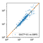
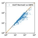
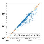
Figure 1: Comparing solution length of GUCT-based algorithms ($x$-axis) against GBFS ($y$-axis) using $h^{\mathrm{FF}}$.

6 Related Work

Due to its focus on adversarial games, MCTS literature typically assumes a bounded reward setting (e.g., 0/1, -1/+1), making applications of UCB1-Normal scarce (e.g., Google Scholar returns 5900 vs. 60 for keyword “UCB1” and “UCB1-Normal”, respectively) except a few model-selection applications (McConachie and Berenson 2018). While Gaussian Process MAB (Srinivas et al. 2010) has been used with MCTS for sequential decision making in continuous space search and robotics (Kim et al. 2020), it is significantly different from discrete search spaces like in classical planning. Bayes-UCT2 (Tesauro, Rajan, and Segal 2010) was only evaluated on a synthetic tree and indeed was often outperformed by the base UCT (Imagawa and Kaneko 2016).

MABs may provide a rigorous theoretical tool to analyze the behavior of a variety of existing randomized enhancements for agile/satisficing search that tackle the exploration-exploitation dilemma. $\epsilon$-greedy GBFS was indeed inspired by MABs (Valenzano et al. 2014, Sec. 2). GUCT-Normal2 encourages exploration in nodes further from the goal, which tend to be close to the initial state. This behavior is similar to that of Diverse Best First Search (Imai and Kishimoto 2011), which stochastically enters an “exploration mode” that expands a node with a smaller $g$ value more often. This reverse ordering is unique from other diversified search algorithms, including $\epsilon$-GBFS, Type-GBFS (Xie, Müller, and Holte 2015), and Softmin-Type-GBFS (Kuroiwa and Beck 2022), which selects $g$ rather uniformly during the exploration.

Theoretical guarantees of MABs require modifications in tree-based algorithms (e.g. MCTS) due to non-i.i.d. sampling from the subtrees (Coquelin and Munos 2007; Munos et al. 2014). Incorporating the methods developed in the MAB community to counter this bias in the subtree samples is an important direction for future work.

MDP and Reinforcement Learning literature often use discounting to avoid the issue of divergent cumulative reward: when the upper bound of step-wise reward is known to be $R$, then the maximum cumulative reward goes to $\infty$ with infinite horizon, while the discounting with $\gamma$ makes it below $\frac{R}{1-\gamma}$, allowing the application of UCB1. Although it addresses the numerical issue and UCB1’s theoretical requirement, it no longer optimizes the cumulative objective.

7 Conclusion

We examined the theoretical assumptions of existing bandit-based exploration mechanisms for classical planning, and showed that ad hoc design decisions can invalidate theoretical guarantees and harm performance. We presented GUCT-Normal2, a classical planning algorithm combining MCTS and UCB1-Normal2, and analyzed it both theoretically and empirically. The theoretical analysis of its regret bound revealed that, despite its worst-case polynomial bound, in practice it outperforms logarithmically-bounded UCB1-Normal due to the unique aspect of the target application (classical planning). Most importantly, GUCT-Normal2 outperforms GBFS, making it the first bandit-based MCTS to outperform traditional algorithms. Future work includes combinations with other enhancements for agile search including novelty metric (Lipovetzky and Geffner 2017), as well as C++ re-implementation and the comparison with the state-of-the-art.

Our study showcases the importance of considering theoretical assumptions when choosing the correct bandit algorithm for a given application. However, this does not imply that UCB1-Normal is the end of the story: for example, while the Gaussian assumption is sufficient for cost-to-go estimates in classical planning, it is not necessary for justifying its application to classical planning. The Gaussian assumption implies that rewards can be any value in $[-\infty,\infty]$, which is an under-specification for non-negative cost-to-go estimates. Future work will explore bandits that reflect the assumptions in classical planning with even greater fidelity.

References

- Alkhazraji et al. (2020) Alkhazraji, Y.; Frorath, M.; Grützner, M.; Helmert, M.; Liebetraut, T.; Mattmüller, R.; Ortlieb, M.; Seipp, J.; Springenberg, T.; Stahl, P.; and Wülfing, J. 2020. Pyperplan. https://doi.org/10.5281/zenodo.3700819. Accessed: 2022-06-08.
- Asai and Fukunaga (2017) Asai, M.; and Fukunaga, A. 2017. Exploration Among and Within Plateaus in Greedy Best-First Search. In Proc. of ICAPS. Pittsburgh, USA.
- Audibert, Munos, and Szepesvári (2009) Audibert, J.-Y.; Munos, R.; and Szepesvári, C. 2009. Exploration–Exploitation Tradeoff using Variance Estimates in Multi-Armed Bandits. Theoretical Computer Science, 410(19): 1876–1902.
- Auer, Cesa-Bianchi, and Fischer (2002) Auer, P.; Cesa-Bianchi, N.; and Fischer, P. 2002. Finite-Time Analysis of the Multiarmed Bandit Problem. Machine Learning, 47(2-3): 235–256.
- Bellemare et al. (2015) Bellemare, M. G.; Naddaf, Y.; Veness, J.; and Bowling, M. 2015. The Arcade Learning Environment: An Evaluation Platform for General Agents (Extended Abstract). In Yang, Q.; and Wooldridge, M. J., eds., Proc. of IJCAI, 4148–4152. AAAI Press.
- Bonet and Geffner (2001) Bonet, B.; and Geffner, H. 2001. Planning as Heuristic Search. Artificial Intelligence, 129(1): 5–33.
- Bush and Mosteller (1953) Bush, R. R.; and Mosteller, F. 1953. A Stochastic Model with Applications to Learning. The Annals of Mathematical Statistics, 559–585.
- Coquelin and Munos (2007) Coquelin, P.-A.; and Munos, R. 2007. Bandit Algorithms for Tree Search. In Proc. of UAI, 67–74.
- Dijkstra (1959) Dijkstra, E. W. 1959. A Note on Two Problems in Connexion with Graphs. Numerische mathematik, 1(1): 269–271.
- Ferber et al. (2022a) Ferber, P.; Cohen, L.; Seipp, J.; and Keller, T. 2022a. Learning and Exploiting Progress States in Greedy Best-First Search. In Proc. of IJCAI.
- Ferber et al. (2022b) Ferber, P.; Geißer, F.; Trevizan, F.; Helmert, M.; and Hoffmann, J. 2022b. Neural Network Heuristic Functions for Classical Planning: Bootstrapping and Comparison to Other Methods. In Proc. of ICAPS.
- Ferber, Helmert, and Hoffmann (2020) Ferber, P.; Helmert, M.; and Hoffmann, J. 2020. Neural Network Heuristics for Classical Planning: A Study of Hyperparameter Space. In Proc. of ECAI, 2346–2353.
- Fikes, Hart, and Nilsson (1972) Fikes, R. E.; Hart, P. E.; and Nilsson, N. J. 1972. Learning and Executing Generalized Robot Plans. Artificial Intelligence, 3(1-3): 251–288.
- Garrett, Kaelbling, and Lozano-Pérez (2016) Garrett, C. R.; Kaelbling, L. P.; and Lozano-Pérez, T. 2016. Learning to Rank for Synthesizing Planning Heuristics. In Proc. of IJCAI, 3089–3095.
- Gehring et al. (2022) Gehring, C.; Asai, M.; Chitnis, R.; Silver, T.; Kaelbling, L. P.; Sohrabi, S.; and Katz, M. 2022. Reinforcement Learning for Classical Planning: Viewing Heuristics as Dense Reward Generators. In Proc. of ICAPS.
- Gelly and Silver (2011) Gelly, S.; and Silver, D. 2011. Monte-Carlo Tree Search and Rapid Action Value Estimation in Computer Go. Artificial Intelligence, 175(11): 1856–1875.
- Hart, Nilsson, and Raphael (1968) Hart, P. E.; Nilsson, N. J.; and Raphael, B. 1968. A Formal Basis for the Heuristic Determination of Minimum Cost Paths. Systems Science and Cybernetics, IEEE Transactions on, 4(2): 100–107.
- Helmert (2006) Helmert, M. 2006. The Fast Downward Planning System. J. Artif. Intell. Res.(JAIR), 26: 191–246.
- Heusner, Keller, and Helmert (2017) Heusner, M.; Keller, T.; and Helmert, M. 2017. Understanding the Search Behaviour of Greedy Best-First Search. In Proc. of SOCS, volume 8.
- Heusner, Keller, and Helmert (2018a) Heusner, M.; Keller, T.; and Helmert, M. 2018a. Best-Case and Worst-Case Behavior of Greedy Best-First Search. In Proc. of IJCAI.
- Heusner, Keller, and Helmert (2018b) Heusner, M.; Keller, T.; and Helmert, M. 2018b. Search Progress and Potentially Expanded States in Greedy Best-First Search. In Proc. of IJCAI.
- Hoffmann and Nebel (2001) Hoffmann, J.; and Nebel, B. 2001. The FF Planning System: Fast Plan Generation through Heuristic Search. J. Artif. Intell. Res.(JAIR), 14: 253–302.
- Imagawa and Kaneko (2016) Imagawa, T.; and Kaneko, T. 2016. Monte carlo tree search with robust exploration. In International Conference on Computers and Games, 34–46. Springer.
- Imai and Kishimoto (2011) Imai, T.; and Kishimoto, A. 2011. A Novel Technique for Avoiding Plateaus of Greedy Best-First Search in Satisficing Planning. In Proc. of AAAI.
- Kaufmann, Cappé, and Garivier (2012) Kaufmann, E.; Cappé, O.; and Garivier, A. 2012. On Bayesian Upper Confidence Bounds for Bandit Problems. In Proc. of AISTATS, 592–600. PMLR.
- Keller and Helmert (2013) Keller, T.; and Helmert, M. 2013. Trial-Based Heuristic Tree Search for Finite Horizon MDPs. In Proc. of ICAPS.
- Kim et al. (2020) Kim, B.; Lee, K.; Lim, S.; Kaelbling, L.; and Lozano-Pérez, T. 2020. Monte Carlo Tree Search in Continuous Spaces using Voronoi Optimistic Optimization with Regret Bounds. In Proc. of AAAI, volume 34, 9916–9924.
- Kishimoto et al. (2022) Kishimoto, A.; Bouneffouf, D.; Marinescu, R.; Ram, P.; Rawat, A.; Wistuba, M.; Palmes, P.; and Botea, A. 2022. Bandit Limited Discrepancy Search and Application to Machine Learning Pipeline Optimization. In Proc. of AAAI, volume 36, 10228–10237.
- Kishimoto, Zhou, and Imai (2012) Kishimoto, A.; Zhou, R.; and Imai, T. 2012. Diverse Depth-First Search in Satisificing Planning. In Proc. of SOCS, volume 3.
- Kocsis and Szepesvári (2006) Kocsis, L.; and Szepesvári, C. 2006. Bandit Based Monte-Carlo Planning. In Proc. of ECML, 282–293. Springer.
- Kuroiwa and Beck (2022) Kuroiwa, R.; and Beck, J. C. 2022. Biased Exploration for Satisficing Heuristic Search. In Proc. of ICAPS.
- Lai, Robbins et al. (1985) Lai, T. L.; Robbins, H.; et al. 1985. Asymptotically Efficient Adaptive Allocation Rules. Advances in Applied Mathematics, 6(1): 4–22.
- Lipovetzky and Geffner (2017) Lipovetzky, N.; and Geffner, H. 2017. Best-First Width Search: Exploration and Exploitation in Classical Planning . In Proc. of AAAI.
- Lipovetzky, Ramírez, and Geffner (2015) Lipovetzky, N.; Ramírez, M.; and Geffner, H. 2015. Classical Planning with Simulators: Results on the Atari Video Games. In Proc. of IJCAI.
- McConachie and Berenson (2018) McConachie, D.; and Berenson, D. 2018. Estimating Model Utility for Deformable Object Manipulation using Multiarmed Bandit Methods. IEEE Transactions on Automation Science and Engineering, 15(3): 967–979.
- Munos et al. (2014) Munos, R.; et al. 2014. From Bandits to Monte-Carlo Tree Search: The Optimistic Principle Applied to Optimization and Planning. Foundations and Trends® in Machine Learning, 7(1): 1–129.
- Nakhost and Müller (2009) Nakhost, H.; and Müller, M. 2009. Monte-Carlo Exploration for Deterministic Planning. In Proc. of IJCAI.
- Richter and Helmert (2009) Richter, S.; and Helmert, M. 2009. Preferred operators and deferred evaluation in satisficing planning. In Proc. of ICAPS, volume 19, 273–280.
- Richter, Westphal, and Helmert (2011) Richter, S.; Westphal, M.; and Helmert, M. 2011. LAMA 2008 and 2011. In Proc. of IPC, 117–124.
- Rivlin, Hazan, and Karpas (2019) Rivlin, O.; Hazan, T.; and Karpas, E. 2019. Generalized Planning With Deep Reinforcement Learning. In Proc. of PRL.
- Robbins (1952) Robbins, H. 1952. Some Aspects of the Sequential Design of Experiments. Bulletin of the American Mathematical Society, 58(5): 527–535.