Spontaneous stochasticity in the presence of intermittency

Abstract

Spontaneous stochasticity is a modern paradigm for turbulent transport at infinite Reynolds numbers. It suggests that tracer particles advected by rough turbulent flows and subject to additional thermal noise, remain non-deterministic in the limit where the random input, namely the thermal noise, vanishes. Here, we investigate the fate of spontaneous stochasticity in the presence of spatial intermittency, with multifractal scaling of the lognormal type, as usually encountered in turbulence studies. In principle, multifractality enhances the underlying roughness, and should also favor the spontaneous stochasticity. This letter exhibits a case with a less intuitive interplay between spontaneous stochasticity and spatial intermittency. We specifically address Lagrangian transport in unidimensional multifractal random flows, obtained by decorating rough Markovian monofractal Gaussian fields with frozen-in-time Gaussian multiplicative chaos. Combining systematic Monte-Carlo simulations and formal stochastic calculations, we evidence a transition between spontaneously stochastic and deterministic behaviors when increasing the level of intermittency. While its key ingredient in the Gaussian setting, roughness here suprisingly conspires against the spontaneous stochasticity of trajectories.

Introduction.

When transported by a sufficiently turbulent flow, puffs of fluid particles are known to undergo a phase of algebraic inflation $R\sim t^{3/2}$, independent from their initial size and now known as Richardson diffusion ^{1; 2; 3; 4; 5; 6; 7; 8; 9; 10}. Beyond the law in itself, Richardson’s seminal contribution is the intuition that turbulent transport requires some probabilistic modeling: The modern interpretation uses the phenomenon of spontaneous stochasticity^{11; 12; 13; 14; 15; 16}, which involves tracers as fluid particles advected by the fluid and subject to additional thermal noise of amplitude $\kappa$ ¹⁷: In the vanishing viscosity limit, the multi-scale nature of turbulent flows amplifies thermal noise in such a drastic fashion, that initially coinciding particles may separate in finite time although their dynamics formally solve the same initial value problem ^{18; 19; 20}, hereby suggesting intrinsic nature for the underlying randomness.
To date, the scenario of spontaneous stochasticity for Lagrangian separation is fully substantiated within the theory of Kraichnan flows. Kraichnan flows are minimal random ersatzes of homogeneous isotropic turbulent fields ^{21; 22; 23; 19; 24; 17}; They are defined as white-in-time Gaussian random fields, whose spatial statistics are centered and prescribed by two-point correlation functions with algebraic decay of the kind

$$C_{\eta}^{(\xi)}(r)=1-|r|^{\xi}\text{ for $\eta\leq|r|\ll 1$},$$ (1)

and vanishing at large scales $\gg 1$. $\eta$ is a scale under which the flow is smooth, analogous to so-called Kolmogorov scale: The scales $\eta\leq|r|\ll 1$ define the so-called inertial range in turbulence theory. The Hurst parameter $\xi\in]0;2[$ prescribes the roughness of the field, through inertial-range scaling $\left\langle(v(x+r)-v(x))^{2}\right\rangle\sim r^{\xi}$. In the limit $\eta\to 0$, this means that the lesser $\xi$, the rougher $v$. In this stochastic setting, spontaneous stochasticity essentially means that some random time accounting for the large-scale $O(1)$ dispersion of a puff of tracers with initial size $O(\eta)$ has probability 1 to be finite in limits where $\eta,\kappa$ jointly vanish. The limit describes puffs initially coalescing to a point in prescribed (quenched) space-time velocity realizations ^{4; 20}. For instance, explicitly considering the relative separation ${\bf R}(t,{\bf r}_{0}):={\bf X}_{2}(t,{\bf x}_{0}+{\bf r}_{0})-{\bf X}_{1}(t,{\bf x}_{0})$ between two tracers initiated at $\bf x_{0},\bf x_{0}+{\bf r}_{0}$, a natural separation time is

$$\tau_{1}(\eta,\kappa):=\inf_{\|{\bf r}_{0}\|=\eta}\left\{t|\|{\bf R}(t,{\bf r}_{0})\|\geq 1\right\}.$$ (2)

from which we interpret spontaneous stochasticity as the property

$$\mathbb{P}\left[\tau_{1}<\infty\right]\to 1\text{ as $\eta,\kappa\to 0$}.$$ (3)

Even at this essential level, the presence or the absence of spontaneous stochasticity in Kraichnan flows depends on a subtle interplay between four parameters: roughness, compressibility, space-dimension, reflection rules for colliding trajectories. To highlight the effect of roughness, we focus on the unidimensional space, hence prescribing unit compressibility, with a thermal noise $\kappa=\eta$ ensuring that colliding trajectories reflect upon collision in the limit $\eta\to 0$. The only relevant parameter is then the roughness exponent $\xi$: Spontaneously stochastic property  (3) holds if and only if $\xi<1$. For $\xi\geq 1$, particles wind up sticking together hence producing apparent deterministic behavior ^{25; 17; 26}: In short, Kraichan flows suggest the mantra “The rougher, the more spontaneously stochastic”. In this letter, we show that this mantra cannot be repeated in the presence of multifractality, a feature which we later also refer to as spatial intermittency.

1D multifractal Kraichnan flows.

We propose a multifractal unidimensional generalization of the Kraichnan model, which prescribes the motion of $N$ tracers particles $(X_{i},i\in[|1;N|])$ in terms of the advection-diffusion

$$dX_{i}=u_{\eta}^{\xi,\gamma}\left(X_{i}(t),dt\right)+\sqrt{2\kappa}\;B_{i}(dt),$$ (4)

where the $B_{i}$’s are independent Brownian motions and we set $\kappa=\eta$ for the thermal noise amplitude: This scaling ensures that close-by tracers separated by at most $\eta$ diffuse away from each other. The smoothing scale $\eta$ will ultimately be taken to $0$. The velocity $u_{\eta}^{\xi,\gamma}$ models turbulent advection in a rough multifractal field, prescribed by the Hurst exponent $\xi\in]0;2[$ and the intermittency parameter $\gamma$. We use the 1D Markovian version of the spatio-temporal fields constructed by Chevillard & Reneuve ²⁷

$$\begin{split}&u^{\xi,\gamma}_{\eta}(x,dt)=\dfrac{1}{Z_{\eta}}\int_{\mathbb{R}}L^{(\xi)}_{\eta}(x-y)\,e^{\gamma Y(y)}W_{1}(dy,dt),\\ &\text{for}\;Y(y):=\int_{\mathbb{R}}L_{\eta}^{(0)}(y-z)W_{2}(dz),\;\;Z:=e^{\gamma^{2}\mathbb{E}\left({Y^{2}}\right)},\end{split}$$ (5)

in terms of the mutually independent (1+1) dimensional Wiener process $W_{1}$ and Brownian motion $W_{2}$, also independent from the $B_{i}$’s. The kernels $L^{(\xi)}_{\eta}$ prescribe the Hurst exponent of the velocity field when $\gamma=0$; They are here defined as convolution square roots of the correlation function

$$C^{(\xi)}(r)=\begin{cases}&\left(1-r^{\xi}\right)\mathbf{1}_{r<1}\text{ for }\xi>0\\ &\left(\log\frac{1}{r}\right)\mathbf{1}_{r<1}\text{ for }\xi=0\end{cases}.$$ (6)

The subscript $\eta$ denotes a regularization over the small-scale $\eta$, in practice most easily defined using Fourier transforms ²⁶. Please note that the expressions (6) indeed represent correlation functions for $0<\xi\leq 1$ ²⁸, and we therefore restrict our analysis to this range. With this choice, Eq.  (1) is then exactly and not just asymptotically satisfied. Spatial intermittency is modeled by the term $M_{\eta}^{(\gamma)}=e^{\gamma Y}W_{1}(dy,\cdot)$, namely the exponentiation of a regularized fractional Gaussian field $Y$ with vanishing Hurst exponent. This non-trivial operation reguires to be suitably normalized by the term $Z=e^{\gamma^{2}\mathbb{E}(Y^{2})}\sim\eta^{-\gamma^{2}}$. The mathematical expectation $\mathbb{E}$ denotes an average over the random environment Y. When $\gamma<\sqrt{2}/2\simeq 0.707$, the limit $\eta\to 0$ then produces a well-defined and non-trivial multifractal random distribution called Gaussian multiplicative chaos ^{29; 30; 31; 32} (later referred to as GMC). The multifractality prescribes the power-law scaling $S_{p}(\ell):=\left\langle|u(x+r)-u(x)|^{p}\right\rangle\sim C_{p}|r|^{\zeta(p)}$ in the inertial range $\eta\leq r\ll 1$, with quadratic variation of the structure function exponents as

$$\begin{split}&\zeta(p)=p\left(\xi/2+\gamma^{2}\right)-\gamma^{2}p^{2}/2;\end{split}$$ (7)

This is a signature of log-normal multifractality – see Fig. 1 for a numerical illustration using Monte-Carlo averaging with $\eta=2^{-20}$, and the power law extending over almost 5 decades.

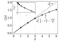
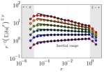
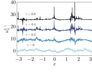
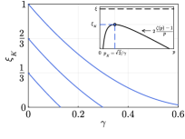
Figure 1: (a) Multifractal prediction given by Eq. (7) for $\gamma=0.2$. Inset shows the correlation function with the power-law decay (1) for $\xi=\zeta(2)$. (b) Compensated structure functions $r^{-\xi}\left\langle|\delta u|^{p}\right\rangle^{2/p}\propto r^{2\zeta(p)/p-\xi}$ for integer orders $1\leq p\leq 6$ (from bottom to top). Points indicate Monte-Carlo averaging over $512$ samples using $N=2^{20}$ points and smoothing scale $\eta=4\pi/N$. The black shaded lines indicate the multifractal prediction. (c) Random realizations of the spatial part of (5) for $\xi=2/3$ and various $\gamma$ . (d) Effective roughess $\xi_{K}$ as a function of $\gamma$ for various $\xi$. Inset illustrates Definition  (8).

Here, the originality of the field (5) comes from its temporal dependence. The Gaussian component is Markovian, and the random environment (5) is analogous to a Kraichnan flow when we set the intermittency parameter $\gamma=0$. The GMC component is random but frozen-in-time: This feature will allow the spatial intermittency to play out in (4) even at the level of two-particle dynamics.

Two wrong intuitive assumptions on multi-scaling & spontaneous stochasticity.

Eq. (7) prescribes $\zeta(2)=\xi$, meaning that for the multifractal fields (5), the two-point correlation (1) is prescribed by the Hurst exponent, independently from the intermittency parameter $\gamma$. Still, our multifractal fields are rougher than their mono-fractal counterpart. This is seen qualitatively from the numerical realizations of Fig. 1 (c): Increasing $\gamma$ also increases the spikiness of the signal. More quantitatively, the spatial roughness $\xi_{K}$ of a single realization of the random field $u^{\xi,\gamma}$ is tied to its scaling exponents $\zeta(p)$ through the classical Kolmogorov continuity theorem ^{33; 34} as

$$\xi_{K}=2\sup_{p}\dfrac{\zeta(p)-1}{p}\leq\xi$$ (8)

For $\gamma=0$, the mono-fractal behavior $\zeta(p)=\ p\xi/2$ holds for arbitrarily large $p$’s, and as such the exponent $\xi_{K}$ identifies to the Hurst exponent $\xi$. For $\gamma\neq 0$, though, this value is reached at $p_{K}=\sqrt{2}/\gamma$, which prescribes $\xi_{K}<\xi$ – see Fig 1 (d). On the one hand, because of this enhanced roughness, one could in principle expect that tracers advected in the intermittent fields (4) are more likely to exhibit non-deterministic behavior than in Kraichnan flows, following the mantra “The rougher, the more spontaneous stochastic”. On the other hand, two-particle separations in the monofractal Kraichnan flows depend only on $\zeta(2)=\xi$ ²⁶: One may as well expect that at least at the level of two-particle separation, one should see no effect of intermittency. We now present some formal and numerical results, to argue that none of the intuitive assumptions formulated above are in fact correct.

From random fields to random potentials.

We focus on the dynamics of pair separations, obtained by considering $N=2$ in Eq. (4). Similar to the Gaussian case ^{35; 36}, tracers advected by Eq. (4) can be interpreted in terms of particles interacting through a random pairwise potential, and whose dynamics are prescribed through the stochastic differential equation (SDE)

$$\begin{split}&dX_{i}=\dfrac{1}{Z_{\eta}}\sum_{j=1,2}L_{ij}\left(|X_{1}-X_{2}|\right)e^{\gamma Y(X_{j})}W_{j}(dt)\\ &\hskip 113.81102pt+\sqrt{2\kappa}B_{i}(dt)\\ &\text{with }L(r):=\begin{pmatrix}&1&0\\ &1-r^{\xi}&\sqrt{1-(1-r^{\xi})^{2}}\\ \end{pmatrix}\end{split}$$ (9)

The matrix $L$ is a discrete analogue to the kernels $L_{\eta}^{(\xi)}$ featured in Eq. (5), except for the regularizing scale $\eta$. It corresponds to an explicit Choleski decomposition of the correlation matrix $C_{2}:=C(|X_{i}-X_{j}|)_{i,j=1,2}$ such that $LL^{T}=C_{2}$. As a SDE version of the original dynamics (4), Eq. (9) comes with two advantages. (i) At a numerical level, it allows for Monte-Carlo sampling of trajectories without the need to generate the fields of Eq. (5) at each time-step, similar to the Gaussian setting ^{35; 36}. (ii) At a formal level, separation-time statistics can be obtained by means of stochastic calculus and potential theory for Markov processes, in other words Feynman-Kac-like formulas. The word formal is advisory, as the frozen-in-time GMC entering the dynamics could require cautious mathematical handling^{31; 37; 38}, but this goes way beyond the scope of the present letter.

The paradoxical interplay between intermittency and spontaneous stochasticity.

Stochastic calculus suggests that for a prescribed realization of the GMC, the pair-separation time $T_{1}^{Y}(r)$ from scale $r$ to scale $1$ formally solves the boundary-value problem

$$\begin{split}&\mathcal{L}_{2}^{Y}T_{1}^{Y}=-1\;\;\;\\ &\text{ with }T_{1}^{Y}(1)=0\text{ and }\partial_{r}T^{Y}_{1}(\eta)=0,\end{split} \gamma$$ (-BVP)

involving the GMC-dependent operator

$$\begin{split}&\mathcal{L}_{2}^{Y}(X_{1},r):=\dfrac{e^{2\gamma Y(X_{1})}}{2Z_{\eta}^{2}}\left(r^{\xi}+e^{2\gamma\Delta Y}\left(2-r^{\xi}\right)\right)r^{\xi}\partial_{rr},\end{split}$$ (10)

which features the increment $\Delta Y:=Y\left(X_{1}+r\right)-Y\left(X_{1}\right)$. For $\gamma\neq 0$, ($\gamma$-BVP) features a non-trivial coupling between the pair-separation time and the underlying GMC. Because of this coupling, ($\gamma$-BVP) is not closed and one cannot a priori solve it explicitly for $T_{1}^{Y}$. Setting $\gamma=0$ retrieves the Gaussian setting and provides a statistical decoupling^{17; 26}, which makes Eq. ($\gamma$-BVP)-(10) solvable. For $\gamma\neq 0$, we define the annealed separation-time

$$\tau_{1}:=\mathbb{E}\left(T_{1}^{Y}\right),$$ (11)

where we recall that the expectation $\mathbb{E}\left(\cdot\right)$ denotes an average over the GMC random environment. A non-trivial decoupling is then obtained under the mean-field Ansatz

$$\mathbb{E}\left(e^{\gamma\Delta Y}T_{1}^{Y}\right)=\mathbb{E}\left(e^{\gamma\Delta Y}\right)\tau_{1}.$$ (12)

For $\eta\ll 1$, ($\gamma$-BVP) under Anzatz (12) formally becomes

$$\begin{split}&\mathcal{L}^{*}_{2}\tau_{1}=-1\;\;\;\text{ with }\tau_{1}(1)=0\text{ and }\partial_{r}\tau_{1}(0)=0,\\ &\text{ for }\mathcal{L}_{2}^{*}(r):=\left(1-\dfrac{r^{\xi}}{2}\right)r^{\xi+4\gamma^{2}}\partial_{rr}.\end{split}$$ (13)

We refer the reader to Supplemental Material ²⁶ for details on derivations of (10)-(13) . As for now, we observe that the term $(1-r^{\xi}/2)$ is bounded and of order $O(1)$. Hence, the separation times behave as if the multifractal random flows were Gaussian, yet with effective driving Hurst parameter

$$\xi_{\gamma}:=\xi+4\gamma^{2}>\xi>\xi_{K}.$$ (14)

This Gaussian flow is smoother than the flow at $\gamma=0$ ! This calculation evidences a highly paradoxical interplay between multifractality, roughness and spontaneous stochasticity: Increasing $\gamma$ makes the flow rougher in terms of the effective roughness $\xi_{K}$ deduced from Kolmogorov theorem, but makes the flow smoother in terms of the spontaneous stochasticity of tracers, driven by $\xi_{\gamma}$ given above. A practical consequence of Eq. (14) is the presence of a phase transition driven by $\gamma$, and characterized by $\xi_{\gamma}=1$. This prescribes the mean-field critical curve

$$\gamma_{c}=\dfrac{1}{2}\sqrt{1-\xi}:$$ (15)

For $0<\xi<1$, tracers are spontaneously stochastic when $\gamma<\gamma_{c}$ and deterministic when $\gamma\geq\gamma_{c}$. For $\xi=1$, the Gaussian case is deterministic, and the critical $\gamma_{c}$ is vanishing, as should be. For $\xi=0$, this prescribes $\gamma_{c}=1/2$, less than the maximum value $\sqrt{2}/2$ allowed for the GMC. The critical value $\gamma_{c}$ can therefore in principle be achieved for any Hurst exponent $\xi\in]0,1]$,

Numerics.

To illustrate the rationale of the prediction (14) and mean-field Ansatz (12), we now report results of Monte-Carlo sampling of pair trajectories, obtained from two different methods, and where we vary the levels of roughness $\xi$, intermittency $\gamma$ and the regularization scale $\eta$. The first method is field-based. It uses direct integration of the dynamics (4) with standard Euler-Maruyama method, and requires to generate a new spatial realization of the field (5) at each timestep. Tracers are then advected by smoothly interpolating the velocity field at their current positions. The second method is SDE-based. It uses the representation (9) in terms of interacting particles and only requires to generate a single field, namely the frozen GMC, per a pair of trajectories. In the SDE setting, in order to enhance numerical stability, we add a callback function ensuring exact reflecting boundary conditions for particles reaching $\eta$.
Beyond the physical parameters $\xi,\gamma,\eta$, both methods require to set values for the field resolutions $N$, the number of trajectory realizations, the timesteps $dt$ – Table 1 lists the essential numerical parameters. To ensure a finite-time completion of the numerical algorithms, we use a maximal time $T_{max}$ over which the numerics are stopped: Our Monte-Carlo sampling therefore does not measure $\tau_{1}(\eta)$ but rather the estimate $\tilde{\tau}_{1}=\left\langle T_{1}^{Y}\wedge T_{max}\right\rangle$.

$\xi$	$\gamma$	$N$	$\eta$	$dt$	$T_{max}$	Realizations
$2/9$ to $1$	$0$ to $0.6$	$2^{7}$ to $2^{14}$	$4\pi/N$	$10^{-4}$	$8$ to $64$	$10^{5}$

Table 1: Numerical parameters for Fig.2 and Fig. 3 for both methods. For SDE-based numerics, realizations are independent while for the field-based numerics, we use minibatches of 100 trajectories to reach $10^{5}$ samples.

Fig. 2 and Fig. 3 summarize our numerical observations, and those prove compatible with the mean-field predictions. As seen from Fig. 2, we monitor two types of behaviors when prescribing $0<\xi<1$. Setting for instance $\xi=2/3$ as in Panels (a,b), we observe that for small $\gamma$, the estimates $\tilde{\tau}_{1}$ converge to finite value, independent from $T_{max}$. Upon decreasing $\eta$, it is found that this value is compatible with the mean-field prediction $\tau_{1}^{mf}(\xi_{\gamma})=\left(2(1-\xi_{\gamma})(1-\xi_{\gamma}/2)\right)^{-1}$ involving the Kraichnan flow estimate with the driving Hurst exponent as input ²⁶. This evidences the spontaneous stochastic nature of separations for small $\gamma$. For large $\gamma$, the apparent convergence of $\tilde{\tau}_{1}$ when decreasing $\eta$ is a numerical artifact, as the limiting value grows with $T_{max}$. This signals deterministic behavior, with the particles not separating in the limit $\eta\to 0$. As such, for all the values of $\xi$ considered in this work, our numerics reflect the presence of a phase transition at finite value of $\gamma$. This is in agreement with our mean-field argument, and substantiates our claim that intermittency here favors deterministic behavior. The onset of deterministic behavior when increasing $\gamma$ is found to be similar when using either field-based or SDE-based numerics. Focusing on the cases $\xi=1/3$ and $\xi=2/3$, we find good compatibility with the mean-field prediction in the latter case and observe deviations in the former case – see Panel (c). As seen from Panel (d), the mean-field prediction accurately captures the transition between deterministic and non-deterministic behaviors for small values of the effective roughness, corresponding to the larger values of $\xi$. The agreement seems to deteriorate for smaller $\xi$. This discrepancy suggests that the mean-field approach becomes inaccurate in the latter regime, but one cannot rule out a defect of the numerics : As $\xi\to 0^{+}$, the paths become very rough, and the Euler-Maruyama scheme may become unfit even when combined with very fine timestepping.

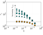
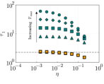
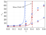
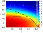
Figure 2: (a) Convergence with $\eta$ of the separation time at $\xi=2/3$ for field-based numerics, using maximal simulation times $T_{max}=8(\triangle),16(\square),32(\diamond),64(\circ)$, for $\gamma=0$ (orange) and $\gamma=0.6$ (green). Dashed line indicates the Kraichnan flow value. (b) Same but for SDE-based numerics. (c) $\tau_{1}$ against $\gamma$ at $\xi=1/3$ (red) and $2/3$ (blue) for field-based ($\circ$) and SDE-based ($\times$) numerics, using the smallest $\eta=10^{-3}$ and largest $T_{max}=64$. (d) Colormap for the average separation time $\tau_{1}$ against the roughness and intermittency parameters $\xi,\gamma$ from SDE-based numerics. Data are normalized by $T_{max}=64$, and interpolated from that measured at the white dots. Red (blue) rendering indicate values close to $0$ (1) suggestive of spontaneously stochastic (deterministic) behavior.

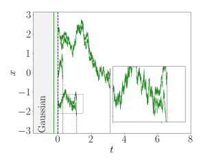
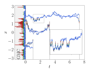
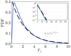
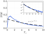
Figure 3: (a) 3 Random realizations of initially coalesced pair trajectories until their separation times $T_{1}$ for driving Hurst parameter $\xi_{\gamma}=2/3$ with $\xi=2/3,\gamma=0$. (b) Same but with $\xi=1/3,\gamma=\sqrt{3}/6.$ Color indicates the magnitude of the underlying GMC, whose profile is represented vertically in the negative axis. (c) PDF of separation-times obtained from SDE-based numerics for $\xi=2/3,\gamma=0$. Inset uses log-scale for the $y$-axis. (b) Same but for $\xi=1/3,\gamma=\sqrt{3}/6$.

Fig. 3 shows the effect of non-Gaussianity playing out at fixed value of the driving Hurst exponent $\xi_{\gamma}=2/3$ in the spontaneous stochastic regime. As seen from Panels (a) and (b), the behaviors between Gaussian and non-Gaussian settings are qualitatively different, although by construction, both share the same mean-field average separation time. In the Gaussian case, the GMC $\propto e^{\gamma Y}$ is unity, and the behavior of pairs is statistically independent from their absolute positions. In the non-Gaussian case, the GMC is non-trivial and we observe a dependence on the local values of the magnitude $\gamma Y$. This is compatible with the fact that Eq. (10) ruling the pair separations is not closed, unless one further averages over the GMC realizations. This behavior reflects in the PDF of exit-times. At large times, the Gaussian setting exhibits the exponential decay $\propto e^{-t/\tau_{1}}$ predicted by the Kraichnan flow theory ²⁶. The non-Gaussian case deviates from the exponential behavior; it exhibits fat tails, likely reflecting particles trapped in quiet “valleys” of the frozen-in-time GMC. Understanding the details of this slow decay requires tools more refined than the present mean-field approach and is left for future studies.

Concluding remarks.

We have proposed a non-trivial extension of the Kraichnan flow theory towards a multifractal setting, that we obtained by decorating the original Markovian Gaussian flows with a frozen-in-time Gaussian multiplicative chaos. Multifractality makes the flow rougher in terms of the Kolmogorov roughness $\xi_{K}$, but the spontaneous stochasticity of two-particle separation maps to that of a smoother Gaussian environment, with Hurst exponent $\xi_{\gamma}>\xi>\xi_{K}$. This paradoxical effect is all the less intuitive, as the second-order structure functions of our parametric family of fields are characterized by constant $\zeta(2)=\xi$ independent of the level of the intermittency. This is an example of a “smoother ride over a rougher sea” at play in scalar transport^{39; 21}, and possibly connected to the mathematical theory of regularization by noise ⁴⁰. The availability of a SDE-based interpretation suggests a new playground to build a fundamental understanding of transport in multifractal environments. This includes tackling higher-dimensions, revisiting scalar intermittency and connections with anomalous dissipation ^{41; 42}, or more generally addressing irreversibility^{43; 44} and universality of transport. On the latter aspect, let us here point out that the specific value of the driving roughness $\xi_{\gamma}$ is clearly model-dependent. For example, using white-in-time versions of the GMC (not shown here), both the mean-field approach and the numerics yield $\xi_{\gamma}=\xi$. The dependence upon time-correlation is reminiscent of that observed in the Gaussian case ²⁰. However, one could expect that the feature $\xi_{\gamma}\geq\zeta(2)$ is a robust feature of pair-dispersion in multifractal environments, and this could prove crucial in assessing transport in genuine turbulent environments. Roughness and intermittency levels measured in 3D homogeneous isotropic turbulence corresponds to $\xi\simeq 0.69$ and $\gamma\simeq 0.15$^{45; 32; 46}. In our model, this choice of parameters results in driving Hurst parameter $\xi_{\gamma}\simeq 0.77$. Transposing this exponent to a deterministic setting would yield Richardson diffusion $R\sim t^{1.62}$, noticeably different from $t^{3/2}$. Naturally, while they extend the Kraichnan flows to a more realistic setting, our unidimensional multifractal environments remain caricatures of genuine turbulent fields, and lack essential ingredients such as skewness, temporal correlations, incompressiblity, etc. At a more mathematical level, our analysis suggests that the problem of transport in multifractal random flows, be them Eq. (5) or variations thereof, might prove solvable. Here, the use of a frozen-in-time GMC as a random environment is strongly reminiscent of the parabolic Anderson model used in condensed matter physics ⁴⁷ and the Liouville Brownian motion entering the construction of field theories in the context of 2D quantum gravity ^{38; 37}. Exploiting those analogies may provide a path towards a rigorous treatment of transport in multifractal turbulent-like random environments, and quantitative modeling of turbulent transport in terms of random fields.

References

- [1] L.F. Richardson. Atmospheric diffusion shown on a distance-neighbour graph. Proc. Roy. Soc. Lond., 110(756):709–737, 1926.
- [2] M.-C. Jullien, J. Paret, and P. Tabeling. Richardson pair dispersion in two-dimensional turbulence. Phys. Rev. Lett., 82(14):2872, 1999.
- [3] G. Boffetta and I. Sokolov. Statistics of two-particle dispersion in two-dimensional turbulence. Phys. Fluids, 14(9):3224–3232, 2002.
- [4] G. Boffetta and I. Sokolov. Relative dispersion in fully developed turbulence: the Richardson’s law and intermittency corrections. Phys. Rev. Lett., 88(9):094501, 2002.
- [5] R. Bitane, H. Homann, and J. Bec. Time scales of turbulent relative dispersion. Phys. Rev. E, 86(4):045302, 2012.
- [6] S. Thalabard, G. Krstulovic, and J. Bec. Turbulent pair dispersion as a continuous-time random walk. J. Fluid Mech., 755:R4, 2014.
- [7] M. Bourgoin. Turbulent pair dispersion as a ballistic cascade phenomenology. J. Fluid Mech., 772:678–704, 2015.
- [8] D. Buaria, B. Sawford, and P-K. Yeung. Characteristics of backward and forward two-particle relative dispersion in turbulence at different Reynolds numbers. Phys. Fluids, 27(10):105101, 2015.
- [9] S. Tan and R. Ni. Universality and intermittency of pair dispersion in turbulence. Phys. Rev. Lett., 128(11):114502, 2022.
- [10] D. Buaria. Comment on “Universality and intermittency of pair dispersion in turbulence”. Phys. Rev. Lett., 130:029401, 2023.
- [11] E. Lorenz. The predictability of a flow which possesses many scales of motion. Tellus, 21(3):289–307, 1969.
- [12] A. Mailybaev. Spontaneously stochastic solutions in one-dimensional inviscid systems. Nonlinearity, 29(8):2238, 2016.
- [13] A. Mailybaev. Spontaneous stochasticity of velocity in turbulence models. Mult. Mod. & Sim., 14(1):96–112, 2016.
- [14] S. Thalabard, J. Bec, and A. Mailybaev. From the butterfly effect to spontaneous stochasticity in singular shear flows. Comm. Phys., 3(1):1–8, 2020.
- [15] A. Mailybaev and A. Raibekas. Spontaneously stochastic Arnold’s cat. Arnold Math. Jour., 2022.
- [16] A. Mailybaev and A. Raibekas. Spontaneous stochasticity and renormalization group in discrete multi-scale dynamics. arXiv preprint arXiv:2207.06158, 2022.
- [17] K. Gawędzki. Soluble models of turbulent transport. In Non-equilibrium statistical mechanics and turbulence, number 355. 2008.
- [18] W. E and E. Vanden Eijnden. Generalized flows, intrinsic stochasticity, and turbulent transport. Proc. Nat. Acad. Sci. U.S.A., 97:8200–8205, 2000.
- [19] A Kupiainen. Nondeterministic dynamics and turbulent transport. Ann. H. Poincaré, 4(2):713–726, 2003.
- [20] M. Chaves, K. Gawędzki, P. Horvai, A. Kupiainen, and M. Vergassola. Lagrangian dispersion in Gaussian self-similar velocity ensembles. J. Stat. Phys., 113(5):643–692, 2003.
- [21] G. Falkovich, K. Gawedzki, and M. Vergassola. Particles and fields in fluid turbulence. Rev. Mod. Phys., 73(4):913, 2001.
- [22] Y. Le Jan and O. Raimond. Integration of Brownian vector fields. Ann. Probab., 30(2):826–873, 2002.
- [23] Y. Le Jan and O. Raimond. Flows, coalescence and noise. Ann. Probab., 32(2):1247–1315, 2004.
- [24] K. Gawędzki. Turbulent advection and breakdown of the Lagrangian flow. In Intermittency in Turbulent Flows.
- [25] K. Gawędzki and M. Vergassola. Phase transition in the passive scalar advection. Phys. D: Nonlin. Phen., 138:63–90, 2000.
- [26] See Supplemental Material for a short reminder on separation times in Kraichnan flow theory, together with explicit details on both the field-based numerics and mean-field calculations.
- [27] J. Reneuve and L. Chevillard. Flow of spatiotemporal turbulent-like random fields. Phys. Rev. Lett., 125(1):014502, 2020.
- [28] A. Yaglom. Correlation Theory of Stationary and Related Random Functions, Volume I: Basic Results, volume 131. Springer, 1987.
- [29] L. Chevillard. Une peinture aléatoire de la turbulence des fluides. HDR thesis, ENS Lyon, 2015.
- [30] R. Pereira, C. Garban, and L. Chevillard. A dissipative random velocity field for fully developed fluid turbulence. J. Fluid Mech., 794:369–408, 2016.
- [31] R. Rhodes and V. Vargas. Gaussian multiplicative chaos and applications: a review. Probab. Surveys, 11:315–392, 2014.
- [32] L. Chevillard, C. Garban, R. Rhodes, and V. Vargas. On a skewed and multifractal unidimensional random field, as a probabilistic representation of Kolmogorov’s views on turbulence. In Ann. H. Poincaré., volume 20, pages 3693–3741. Springer, 2019.
- [33] J.-F. Le Gall. Brownian motion, martingales, and stochastic calculus. Springer, 2016.
- [34] L. Evans. An introduction to stochastic differential equations, volume 82. Am. Math. Soc., 2012.
- [35] U. Frisch, A. Mazzino, and M. Vergassola. Intermittency in passive scalar advection. Phys. Rev. Lett., 80(25):5532, 1998.
- [36] O. Gat, I. Procaccia, and R. Zeitak. Anomalous scaling in passive scalar advection: Monte-Carlo Lagrangian trajectories. Phys. Rev. Lett., 80(25):5536, 1998.
- [37] C. Garban, R. Rhodes, and V. Vargas. Liouville Brownian motion. Ann. Probab., pages 3076–3110, 2016.
- [38] R. Rhodes and V. Vargas. Lecture notes on Gaussian multiplicative chaos and Liouville quantum gravity. arXiv preprint arXiv:1602.07323, 2016.
- [39] U. Frisch and V. Zheligovsky. A very smooth ride in a rough sea. Comm. Math. Phys., 326:499–505, 2014.
- [40] L. Galeati and M. Gubinelli. Noiseless regularisation by noise. Rev. Mat. Ib., 38(2):433–502, 2021.
- [41] T. Drivas and G. Eyink. A Lagrangian fluctuation–dissipation relation for scalar turbulence. part i. flows with no bounding walls. J. Fluid Mech., 829:153–189, 2017.
- [42] N. Valade, S. Thalabard, and J. Bec. Anomalous dissipation and spontaneous stochasticity in deterministic surface quasi-geostrophic flow. In Ann. H. Poincaré, pages 1–23. Springer, 2023.
- [43] M. Bauer and D. Bernard. Sailing the deep blue sea of decaying Burgers turbulence. J. Phys. A: Math. Gen., 32(28):5179, 1999.
- [44] G. Eyink and T. Drivas. Spontaneous stochasticity and anomalous dissipation for Burgers equation. J. Stat. Phys., 158:386–432, 2015.
- [45] B. Dubrulle. Intermittency in fully developed turbulence: Log-Poisson statistics and generalized scale covariance. Phys. Rev. Lett., 73(7):959, 1994.
- [46] A. Mailybaev and S. Thalabard. Hidden scale invariance in Navier–Stokes intermittency. Phil. Trans. Roy. Soc. A, 380(2218):20210098, 2022.
- [47] W. König and T. Wolff. The parabolic Anderson model. Preprint. Available at www. wiasberlin. de/people/koenig, 2015.