Reinforcement Learning for Safe Robot Control
using Control Lyapunov Barrier Functions

Abstract

Reinforcement learning (RL) exhibits impressive performance when managing complicated control tasks for robots. However, its wide application to physical robots is limited by the absence of strong safety guarantees. To overcome this challenge, this paper explores the control Lyapunov barrier function (CLBF) to analyze the safety and reachability solely based on data without explicitly employing a dynamic model. We also proposed the Lyapunov barrier actor-critic (LBAC), a model-free RL algorithm, to search for a controller that satisfies the data-based approximation of the safety and reachability conditions. The proposed approach is demonstrated through simulation and real-world robot control experiments, i.e., a 2D quadrotor navigation task. The experimental findings reveal this approach’s effectiveness in reachability and safety, surpassing other model-free RL methods.

I Introduction

Reinforcement learning (RL) has achieved impressive and promising results in robotics, such as manipulation [1], unmanned vehicle navigation [2], drone flight [3, 4], etc., thanks to its ability of handling intricate models and adapting to diverse problem scenarios with ease. Meanwhile, a safe control policy is imperative for a robot in the real world, as dangerous behaviors can cause irreparable damage or costly losses. Therefore, the RL methods that can provide a safety guarantee for robot control have received considerable interest and progress [5, 6, 7, 8, 9, 10].

A recent line of work focuses on designing novel RL algorithms, e.g., actor-critic, for constrained Markov Decision Process (CMDP). In these methods, the system encourages the satisfaction of the constraints by adding a constant penalty to the objective function [6] or constructing safety critics while doing policy optimization in a multi-objective manner [5, 7, 11, 12]. Although these approaches are attractive for their generality and simplicity, they either need model [6], or only encourage the safety constraints to be satisfied probabilistically.

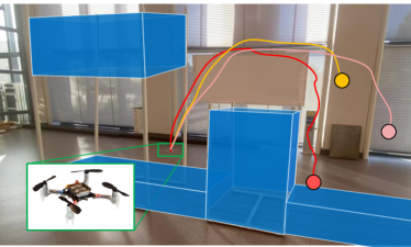
Figure 1: The 2D quadrotor navigation task. Lines stand for trajectories. The circles are the initial position. The blue regions represent obstacles. Video is available at https://youtu.be/_8Yr_QRRYik.

An alternative type of methods focuses on reachability and safety guarantee (sufficient conditions) by constructing/learning control Lyapunov functions (CLF) and control barrier functions (CBF) that can respectively certify the reachability and safety [8, 10, 13, 14, 15, 16, 17, 18]. The relevant safe controllers are normally designed by adding a safety filter to a reference controller, such as a RL controller [8, 10, 13], a model predictive control (MPC) controller [14], etc. Unfortunately, these approaches have two disadvantages: (1) there might be conflicts between CLFs and CBFs as separate certificates [19, 20] (see Figure 2 in Section V-A); (2) the CLFs and CBFs are generally non-trivial to find [19], especially for nonlinear systems. Even though there are learning methods to find CLFs and CBFs, knowledge of dynamic models has to be explicitly used [21].

In this paper, we propose a data-based reachability and safety theorem without explicitly using the knowledge of a dynamic system model. The contribution of this paper can be summarized as follows: (1) we used samples to approximate the critic as a control Lyapunov barrier function (CLBF), a single unified certificate, which is parameterized by deep neural networks, so as to guarantee both reachability and safety. The corresponding actor is a controller that satisfies both the reachability and safety guarantees. (2) we deploy the learned controller to a real-world robot, i.e., a Crazyflie 2.0 quadrotor, for a 2D quadrotor navigation task. The 2D quadrotor navigation task is shown as in Figure 1. The experiments show our approach has better performance than other model-free RL methods. Our approach, by using CLBFs, can avoid conflicts between the CLFs and CBFs certificates. Compared to the model-based approaches that learn CLBFs using supervised learning [19] or handcraft CLBFs [22], our method does not need the knowledge of models explicitly.

II Related Works

Prior work has studied safety in RL in several ways, including imposing constraints on expected return [5, 7], risk measures such as Conditional Value at Risk and percentile estimates [12, 23, 24], and avoiding regions where constraints are violated [25, 26, 27]. This paper focuses on the reach-avoid problem that belongs to the last situation.

To solve the reach-avoid problem, a popular strategy involves modifying the policy optimization procedure of standard RL algorithms to reason about task rewards and constraints simultaneously. One method is constrained policy optimization (CPO), which adds a constraint-related cost to the policy objective [5]. Another type of method tries to optimize a Lagrangian relaxation [7, 11, 23, 27, 28]. They normally use a safety critic to ensure safety, but this separate critic can only evaluate risk in a probabilistic way. Other methods involve constructing Lyapunov functions for the unsafe region [29, 30]. However, these approaches require a baseline policy that already satisfies the constraints.

III Preliminaries and Background

In RL for safe control, the dynamical system is typically characterized by CMDP $\hat{M}=(\mathcal{S},\mathcal{A},P,c,\gamma,\mathcal{I})$ [31]. $s_{t}\in\mathcal{S}\subseteq\mathbb{R}^{n}$ is the state vector at time $t$, $S$ denotes the state space. The agent then takes an action $a_{t}\in\mathcal{A}\subseteq\mathbb{R}^{m}$ according to a stochastic policy/controller $\pi\left(a_{t}\mid s_{t}\right)$. The transition of the state is dominated by the transition probability density function $P\left(s_{t+1}\mid s_{t},a_{t}\right)$, which denotes the probability density of the next state $s_{t+1}$. A cost function $c(s_{t},a_{t})$ is used to measure the immediate performance of a state-action pair $(s_{t},a_{t})$, and $\mathcal{I}(s_{t})$ indicates whether the state violates the safety constraints or not. The goal is to find $\pi^{*}$ that can minimize the objective function return the expected return $J(\pi)\triangleq\sum_{t=1}^{\infty}\mathbb{E}_{s_{t},a_{t}}\gamma^{t}c\left(s_{t},a_{t}\right)$ with the discount factor $\gamma\in[0,1)$, and $\forall t\in\mathbb{Z}_{+},\mathcal{I}(s_{t})=0$. Moreover, some notations are to be defined. The closed-loop state distribution at a certain instant $t$ as $p(s\mid\rho,\pi,t)$, which can be defined iteratively: $p\left(s^{\prime}\mid\rho,\pi,t+1\right)=\int_{\mathcal{S}}P(s^{\prime}|s,\pi(s))p(s\mid\rho,\pi,t)\mathrm{d}s,\forall t\in\mathbb{Z}_{+}$ and $p(s\mid\rho,\pi,0)=\rho(s)$.

In this paper, we focus on the reach-avoid problems, in which the agent reaches the goal condition and avoids certain unsafe conditions. It is defined as follows:

Definition 1.

(Reach-Avoid Problem). In a CMDP setting with a goal configuration $s_{\text{goal}}$ and a set of unsafe states $\mathcal{S}_{\text{unsafe}}\subseteq\mathcal{S}$, find a controller $\pi^{*}\left(a|s\right)$ such that all trajectories $s_{t}$ under $P\left(s_{t+1}\mid s_{t},a_{t}\right)$, and $s_{0}\in\mathcal{S}_{\text{initial}}\subseteq\mathcal{S}$ have the following properties: Reachability: given a tolerance $\delta$, $\exists T\geq 0$, such that $\mathbb{E}_{s_{t}}\left\|s_{t}-s_{\text{goal}}\right\|\leq\delta$, $\forall t\geq t_{0}+T$; Safety: $\mathbb{P}(s_{t}\notin\mathcal{S}_{\text{unsafe}}\mid s_{0},\pi,t)=\int_{\mathcal{S}\setminus\mathcal{S}_{\text{unsafe}}}p(s\mid s_{0},\pi,t)\mathrm{d}s=0$, $\forall t\geq t_{0}$.

The state $s_{\text{irrecoverable}}\in\mathcal{S}_{\text{\text{irrecoverable}}}\not\subset\mathcal{S}_{\text{unsafe}}$ are not themselves unsafe, but inevitably lead to unsafe states under the controller $\pi$. Thus, we also consider $s_{\text{irrecoverable}}$ to be unsafe for the given controller $\pi$.

Definition 2.

A state is said to be irrecoverable if $s\notin\mathcal{S_{\text{unsafe}}}$ under the controller $a\sim\pi(a|s)$, the trajectory defined by $s_{0}=s$ and $s_{t+1}\sim P(s_{t+1}|s_{t},\pi(s_{t}))$ satisfies $\mathbb{P}(s_{t}\in\mathcal{S}_{\text{unsafe}}\mid s_{0},\pi,t)=\int_{\mathcal{S}_{\text{unsafe}}}p(s\mid s_{0},\pi,t)\mathrm{d}s\neq 0$, $\exists\hat{t}>t_{0}$.

Therefore, the safety and unsafety of a certain state can be described as: the state $s\in\mathcal{S}_{\overline{\text{unsafe}}}=\mathcal{S}_{\text{irrecoverable}}\cup\mathcal{S}_{\text{unsafe}}$ is unsafe, while the state $s\in\mathcal{S}_{\overline{\text{safe}}}=\mathcal{S}\backslash\mathcal{S}_{\overline{\text{unsafe}}}$ is safe.

In reach-avoid problems, CLFs and CBFs are widely used to ensure reachability and safety of the system [21], respectively. To avoid the conflicts between separate certificates, we rely on the CLBF, a single unifying certificate for both reachability and safety [22]. In this paper, the definition of the CLBF is related to [19]. We extend it from a continuous-time system to CMDP (similar to the definition of CBF in discrete-time system [32]). In CMDP, the definition of CLBF is given as follows.

Definition 3.

(CLBF). A function V: $\mathcal{S}\rightarrow\mathbb{R}$ is a CLBF, for some constant $\hat{c}$, $\lambda>0$, ① $V\left(s_{\text{goal}}\right)=0$, ② $V(s)>0,\forall s\in\mathcal{S}\backslash\mathcal{S}_{\text{goal}}$, ③ $V(s)\geq\hat{c},\forall s\in\mathcal{S}_{\overline{\text{unsafe}}}$, ④ $V(s)<\hat{c},\forall s\in\mathcal{S}_{\overline{\text{safe}}}$. ⑤ there exists a controller $\pi$, such that $\mathbb{E}_{s^{\prime}}[V\left(s^{\prime}\right)-V(s)+\lambda V(s)]\leq 0,\forall s\in\mathcal{S}\backslash s_{\text{goal}}$, where $s^{\prime}\sim P(s^{\prime}|s,\pi(s))$.

Thus, any controller $\pi\in\{\pi\mid\mathbb{E}_{s^{\prime}}[V(s^{\prime})-V(s)+\lambda V(s)]\leq 0,s^{\prime}\sim P(s^{\prime}|s,\pi(s))\}$ can satisfy reachability and safety [19]. In this definition, the transition $P(s^{\prime}|s,\pi(s))$ requires the knowledge of a dynamic system model, but modeling error can hardly be avoided in reality. Next, we will show how we can use model-free RL to learn CLBFs and controllers with reachability and safety guarantee.

IV Reinforcement Learning Algorithm with Safety Guarantee

In an actor-critc framework, the high-level plan is as follows. We first choose the value function $V(s)$ to be the CLBF, similar to those done in approximate/adaptive dynamic programming [33] on choosing the Lyapunov function. Then we expect to impose some properties of CLBF as constraints in the Bellman recursion to find the value function (i.e., CLBF) and hope to search the corresponding policy, similar to what is done in [25, 29, 34]. Conceptually, we are interested in the following conceptual problem formulation:

Repeat

• Find: V. Subject to: CLBF constraints

• Find: $\pi$ using V

Untill V, $\pi$ convergence.

IV-A CLBF as Critic

To enable the actor-critic learning, the control Lyapunov barrier critic $Q_{\text{LB}}$ is designed to be dependent on $s$ and $a$, while $V(s)=Q_{\text{LB}}(s,\pi_{\theta}(s))$. Then we present a method to construct a $Q_{\text{LB}}$ through the Bellman recursion. The target function $Q_{\text{target}}$ is a valid control Lyapunov barrier critic which is approximated by:

$$Q_{\text{target }}(s_{t},a_{t})=c(s_{t},a_{t})+\gamma Q_{\text{LB}}^{\prime}\left(s_{t+1},\pi(s_{t+1})\right)$$ (1)

where $Q_{\text{LB}}^{\prime}$ is the network that has the same structure as $Q_{\text{LB}}$, but parameterized by a different set $\phi^{\prime}$, as typically used in the actor-critic methods [35, 36]. The parameter $\phi^{\prime}$ is updated through exponential moving average of weights controlled by a hyperparameter $\tau\in\mathbb{R}_{(0,1)},\phi_{k+1}^{\prime}\leftarrow\tau\phi_{k}+(1-\tau)\phi_{k}^{\prime}$.

Such that the value function meets the requirements of our main theorem (Theorem 1 in Section IV-B), the tuples $\{s_{t},a_{t},c(s_{t},a_{t}),s_{t+1}\}$ are set as follows:

$$\begin{cases}\{s_{t},a_{t},0,s_{t}\}&s_{t}\in\mathcal{S}_{\text{goal}}\\ \{s_{t},a_{t},c(s_{t},a_{t}),s_{t+1}\}&s_{t}\in\mathcal{S}_{\text{safe}}\setminus\mathcal{S}_{\text{goal}}\\ \{s_{t},a_{t},C,s_{t}\}&s_{t}\in\mathcal{S}_{\text{unsafe }}\end{cases}$$ (2)

where the terminal cost $C$ is a constant.

IV-B Data-based CLBF Theorem

In this part, inspired by Definition 3 of CLBF, we propose a novel data-based theorem, on which the constraints should be in the conceptual problem formulation at the beginning of Section IV. Instead of explicitly using a dynamic model, the following theorem provides a sufficient condition for reachability and safety based on samples.

Before presenting the main theorem, we need the following Lemma 1, in addition to (2), on the terminal cost $C$ to hold, so that $V(s_{\overline{\text{unsafe}}})\geq\hat{c}$ and $V(s_{\overline{\text{safe}}})<\hat{c}$, as required in (3).

Lemma 1.

Suppose that $N$ is the maximum number of steps in each episode, let $C>\frac{c_{\max}(s,a)\left(1-\gamma^{N}\right)}{\gamma^{N}}$, when $\gamma<1$. Under the controller $\pi$, if $s\in\mathcal{S}_{\overline{\text{unsafe}}}$ , $V(s)\geq\hat{c}$, and $s\in\mathcal{S}_{\overline{\text{safe}}}$  , $V(s)<\hat{c}$.

Proof.

The proof can be found in Appendix A. ∎

Theorem 1.

If there exists a function $V(s):\mathcal{S}\rightarrow\mathbb{R_{+}}$ and positive constants $\alpha_{1}$, $\alpha_{2}$, $\alpha_{3}$, $\alpha_{4}$, such that

$$\begin{aligned} \alpha_{1}c_{\pi}(s)\leq&V(s)<\min{(\alpha_{2}c_{\pi}(s),\hat{c})}<\hat{c},\ \ \ \ \ \ \ \forall s\in\mathcal{S}_{\overline{\text{safe}}}\\ \hat{c}\leq&V(s)\leq\hat{c}+\alpha_{3}c_{\pi}(s)<(1+\alpha_{3})\hat{c},\ \ \forall s\in\mathcal{S}_{\overline{\text{unsafe}}}\end{aligned}$$ (3)

and

$$\begin{aligned} &\mathbb{E}_{s\sim\mu_{N}}\left(\mathbb{E}_{s^{\prime}\sim P_{\pi}}V(s^{\prime})\mathds{1}_{\Delta}(s^{\prime})-V(s)\mathds{1}_{\Delta}(s)\right)\\ &<-\alpha_{4}\mathbb{E}_{s\sim\mu_{N}}c_{\pi}(s)\mathds{1}_{\Delta}(s)\end{aligned}$$ (4)

where $c_{\pi}\left(s_{t}\right)\triangleq\mathbb{E}_{a\sim\pi}c\left(s_{t},a_{t}\right)$, and $c_{\pi}\left(s\right)\leq\hat{c},\forall s\in\mathcal{S}$. The cost function $c(s_{t},a_{t})=\mathbb{E}_{P\left(\cdot\mid s_{t},a_{t}\right)}\left\|s_{t+1}-s_{goal}\right\|$ describes the distance to the goal set. $\mu_{N}(s)$ denotes the average distribution of $s$ over the finite $N$ time steps,

$$\mu_{N}(s)\doteq\frac{1}{N}\sum_{t=1}^{N}p(s|\rho,\pi,t)$$

$N$ is the maximum number of steps in each episode. $\mathds{1}_{\Delta}(s)$ denotes the function;

$$\mathds{1}_{\Delta}(s)=\left\{\begin{array}[]{cc}1&s\in\Delta\\ 0&s\notin\Delta\end{array}\right.$$

where $\Delta=\mathcal{S}\backslash\left(\mathcal{S}_{\text{goal}}\cup\mathcal{S}_{\text{unsafe}}\right)$, $\mathcal{S}_{\text{goal}}=\left\{s\mid c_{\pi}(s)\leq\delta\right\}=\left\{s\mid\left\|s-s_{\text{goal}}\right\|\leq\delta\right\}$. Note that $c_{\pi}(s)>\delta$, $\forall s\in\Delta$.

Then the followings hold: i) if $s_{0}\in\mathcal{S}_{\overline{\text{safe}}},V(s_{0})\leq\hat{c}$, the system is reachable with tolerance $\delta$ and safe within $N$ steps; ii) if $s_{0}\in\mathcal{S}_{\overline{\text{unsafe}}},V(s_{0})>\hat{c}$, the agent would reach the unsafe areas within $N$ steps.

Proof.

The proof can be found in Appendix B. ∎

IV-C Lyapunov Barrier Actor-Critic Algorithm

Recent advance in [34] has guaranteed reachability by the Lagrangian relaxation method. Taking inspiration from their work, we extend to safety guarantee by designing an actor-critic RL algorithm. The proposed Algorithm 1 is named Lyapunov barrier actor-critic (LBAC), which gains a value function that satisfies the requirements of Theorem 1, and a corresponding safe controller.

The control Lyapunov barrier critic function $Q_{\text{LB}}$ and the actor function (controller) $\pi_{\theta}(a_{t}|s_{t})$ are parametrized by $\phi$ and $\theta$, respectively. Note that the stochastic controller $\pi_{\theta}$ is parameterized by a deep neural network $f_{\theta}$ that depends on $s$ and Gaussian noise $\epsilon$. The goal is to construct the CLBF as the critic function with constraints (4) under the controller $\pi_{\theta}(a_{t}|s_{t})$. By using the Lagrange relaxation technique [37], $Q_{\text{LB}}$ is updated using gradient descent to minimize the following objective function

$$J(\phi )=\mathbb{E}_{\mathcal{D}}\left[\frac{1}{2}\left(Q_{\text{LB}}(s,a)-Q_{\text{target}}(s,a)\right)^{2}\right.$$ (5)

$$\left.+\lambda(Q_{\text{LB}}(s^{\prime},f_{\theta}(\epsilon,s^{\prime}))\mathds{1}_{\Delta}(s^{\prime})-Q_{\text{LB}}(s,a)\mathds{1}_{\Delta}(s)+\alpha_{4}\hat{c})\right]$$

where $Q_{\text{target}}$ is the approximation target related to the chosen control Lyapunov barrier candidate, $\lambda$ is a Lagrange multiplier that controls the relative importance of the inequality condition (4). $\mathcal{D}$ is the set of collected transition pairs that are determined in (2) and Lemma 1. The control Lyapunov barrier candidate acts as a supervision signal to the control Lyapunov barrier critic function.

LBAC is based on the maximum entropy framework [36], which can improve controller exploration during learning. A minimum entropy constraint is added to the above optimization problem to derive the following objective function

$$J(\theta)= \mathbb{E}_{(s,a,s^{\prime},c)\sim\mathcal{D}}[Q_{LB}(s,f_{\theta}(\epsilon,s))$$ (6)

$$+\beta(\log(\pi_{\theta}(f_{\theta}(\epsilon,s)|s))+\mathcal{H}_{t}))]$$

where $\beta$ is a Lagrange multiplier that controls the relative importance of the minimum entropy constraint, $\mathcal{H}_{t}$ is the desired entropy bound.

In the actor-critic framework, the parameters of the controller are updated through stochastic gradient descent, which is approximated by

$$\nabla_{\theta}J(\theta) =\beta\nabla_{\theta}\log(\pi_{\theta}(a|s))+\beta\nabla_{a}\log(\pi_{\theta}(a|s))\nabla_{\theta}f_{\theta}(\epsilon,s)$$ (7)

$$+\nabla_{a^{\prime}}Q_{\text{LB}}(s^{\prime},a^{\prime})\nabla_{\theta}f_{\theta}(\epsilon,s^{\prime})$$

Finally, the values of Lagrange multipliers $\lambda$ and $\beta$ are adjusted by gradient ascent to maximize the following objectives, respectively,

$$J(\lambda) =\lambda\mathbb{E}_{\mathcal{D}_{\Delta}}\left[Q_{\text{LB}}\left(s^{\prime},f_{\theta}\left(s^{\prime},\epsilon\right)\right)\mathds{1}_{\Delta}\left(s^{\prime}\right)\right.$$ (8)

$$\left.-\left(Q_{\text{LB}}(s,a)-\alpha_{4}\hat{c}\right)\mathds{1}_{\Delta}(s)\right],$$

$$J(\beta) =\beta\mathbb{E}_{\mathcal{D}}\left[\log\pi_{\theta}(a\mid s)+\mathcal{H}_{t}\right]$$

During training, the Lagrange multipliers are updated by

$$\lambda\leftarrow\max(0,\lambda+\bar{\delta}\nabla_{\lambda}J(\lambda)),\ \ \ \ \beta\leftarrow\max(0,\beta+\bar{\delta}\nabla_{\beta}J(\beta))$$

where $\bar{\delta}$ is the learning rate. The pseudocode of the proposed algorithm is shown in Algorithm 1.

Algorithm 1 Lyapunov Barrier Actor-Critic (LBAC)

0:  Maximum episode length $N$; maximum iteration steps $M$

  repeat

     Sample $s_{0}$ according to $\rho$

     for $t=0$ to $N$ do

        Sample $a_{t}$ from $\pi_{\theta}(a_{t}|s_{t})$ and step forward

        Observe $s_{t+1}$, $c_{t}$ and store $(s_{t},a_{t},c_{t},s_{t+1},\mathcal{I})$ in $\mathcal{D}$

     end for

     for $i=1$ to $M$ do

        Sample mini-batches of transitions from $\mathcal{D}$ and update $Q_{\text{LB}}$, $\pi$, Lagrange multipliers with (5), (6), (8)

     end for

  until (4) is satisfied

V Results and Validation

In this section, we consider a 2D quadrotor navigation task, i.e., aiming to reach a target while avoiding obstacles, as illustrated in Figure 1. The experiment setup is detailed in Appendix C. First, we show separate CLFs and CBFs can lead to local optimums by implementing a CLF-CBF based Quadratic Program (CLF-CBF-QP). Then, we show the effectiveness of the proposed LBAC algorithm and evaluate it in the following aspects:

• Training convergence: does the proposed training algorithm converge with random parameter initialization;

• Validation of CLBF: how do the learned CLBFs fit the goal and obstacles in the 2D quadrotor navigation task, and does the reachability and safety condition, i.e., Theorem 1, hold for the learned controllers;

• Sim-to-Real transfer: can we transfer the simulation training result directly to real-world robots, e.g., using a CrazyFlie 2.0 quadrotor.

In this part, the performance of LBAC on the CMDP tasks is evaluated compared with Risk Sensitive Policy Optimization (RSPO) [23], Safety Q-Functions for RL (SQRL) [11], and Reward Constrained Policy Optimization (RCPO) [7]. We use the public codebase of [27] to implement the comparison experiments. The hyperparameters are described in Appendix D.

V-A Conflicts between CLFs and CBFs

To show there exist conflicts between CLFs and CBFs as separate certificates, we implemented a model-based CLF-CBF-QP controller [38] which incorporates a CLF and CBFs as constraints through quadratic programs. As shown in Figure 2(b), the quadrotor easily gets stuck before the wall which is in front of the target. This is because the attraction of the CLF is balanced by the repulsion of CBFs, as illustrated by Figure 2(a). The quadrotor can still successfully reach the target if it luckily avoids conflicting areas. We also tried CLFs and CBFs as separate critics in a multi-objective RL setting, but failed to converge. The failure of the above CLF-CBF controllers motivates our CLBF approach which satisfies both safety and reachability in this 2D quadrotor navigation task, as illustrated in Figure 7(a).

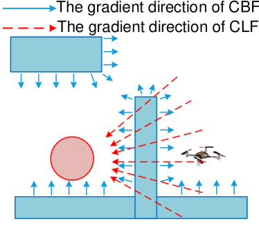
(a) Illustration of CLF-CBF

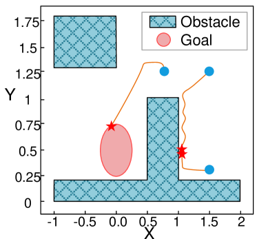
(b) Results of CLF-CBF-QP

Figure 2: Performance of a CLF-CBF-QP controller. (a) is an intuitive illustration of CLF-CBF. In (b), lines are trajectories. The blue circles stand for the starting points. The red stars represent the final position.

V-B Training Convergence

The main criterion we are interested in is the convergence of the controller during the training process. Each approach is trained with five different random seeds. The total cost and number of violations during training are plotted in Figure 3. Among the RL algorithms to be compared, LBAC, RSPO, and SQRL can converge within $2300$ episodes, while RCPO fails to converge even in $3000$ episodes. As shown in Figure 3, LBAC leads to a fewer number of violations during training than other model-free safe RL methods.

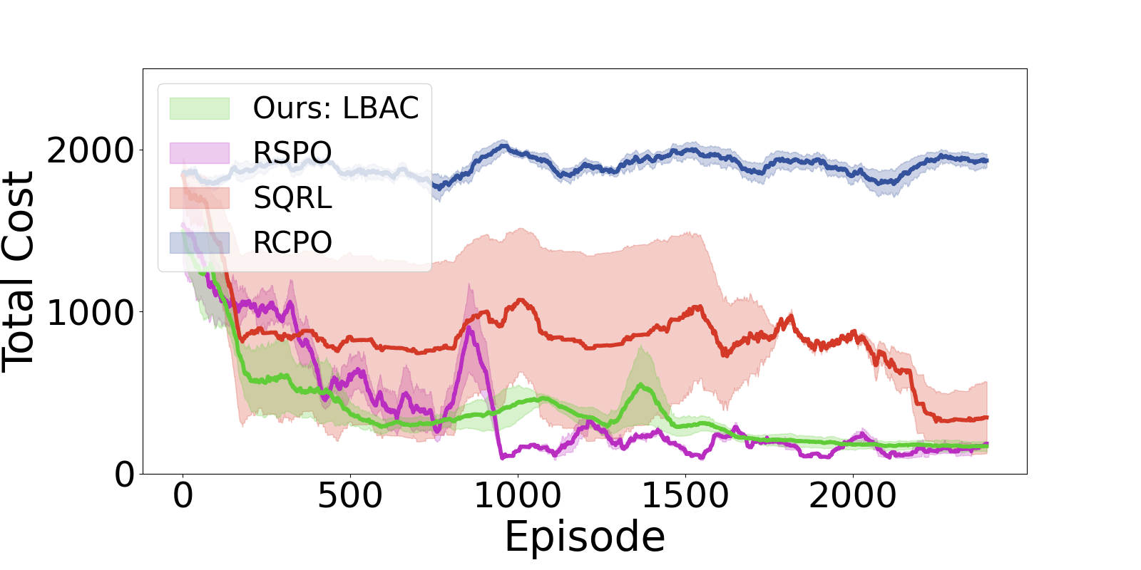
(a) Total Cost

(b) Training-time violations

Figure 3: Total cost and the number of violations during training. The Y-axis indicates the total cost in one episode in (a) and total violation times during training in (b). The X-axis indicates the total episodes. The shaded region shows the 1-SD confidence interval of five random seeds.

V-C Validation of CLBF

In this part, we examine the learned control Lyapunov barrier critic function. We pick the controllers and corresponding CLBFs trained in 1000, 1500, and 2000 episodes. The contour plots of the CLBFs are shown in Figure 4 as a function of $x$ and $y$, where $\{v_{x},v_{y}\}$ is set to $\{0,0\}$. The white lines are the safety boundaries of the CLBFs, i.e. when $V(s)=\hat{c}$ and $\hat{c}$ is set 2000. As shown in Figure 4, we find that the safety boundary of CLBF where $V(s)=\hat{c}$ gradually approaches the obstacle boundary with increasing training episodes. However, we also noticed some unsafe corner cases are considered as safe (such as the bottom right corner of the left obstacle). This could be due to the exploration and exploitation dilemma LBAC suffers as a model-free RL algorithm.

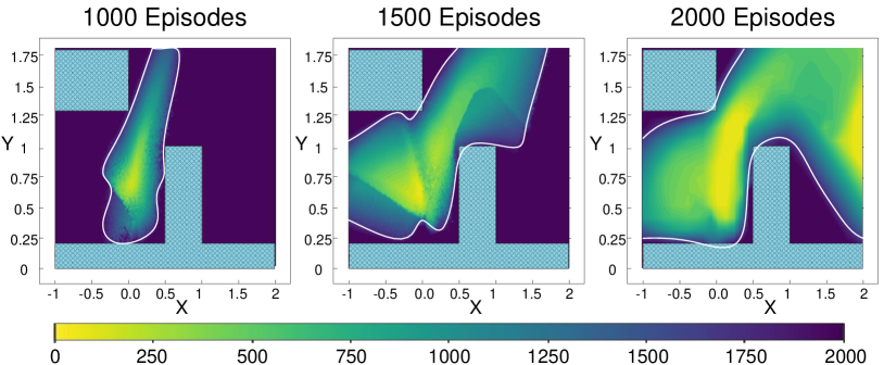
Figure 4: The contour plots of the CLBF. The white lines show the contour of the learned CLBF. The color bar denotes the function value. From left to right, the contour plots are the CLBFs trained in 1000 episodes, 1500 episodes and 2000 episodes.

We also validate the learned CLBF by showing the outcomes of the trajectory rollouts starting from uniformly sampled initial positions. This is because of the well-known fact that it is challenging to initialize uniformly throughout the state space in a model-free setting. For example, we can hardly make a robot have a specific velocity at a particular position. Figure 5 shows that the quadrotors starting from the unsafe region would be violating, while those that start in the safe region would successfully reach the goal. We present the changes in CLBF values along the trajectories in Figure 6(a), and the averaged changes in CLBF value of these trajectories in Figure 6(b). We can observe that the averaged value has a decreasing trend, which aligns with the theory before. These results indicate that the learned CLBF is valid.

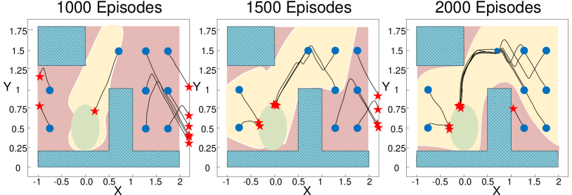
Figure 5: Trajectories of the learned LBAC controllers in the simulator. The shaded area corresponds to the unsafe region. The green ellipse area stands for the goal. The blue circles are the initial positions, while the red stars are the end positions.

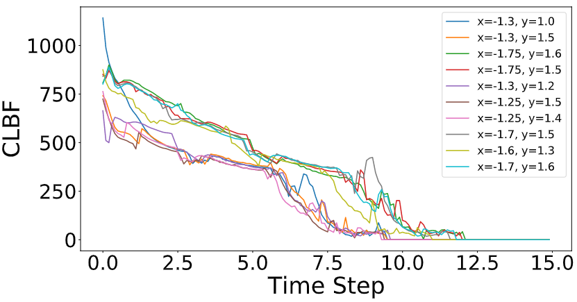
(a) The changes in CLBF value

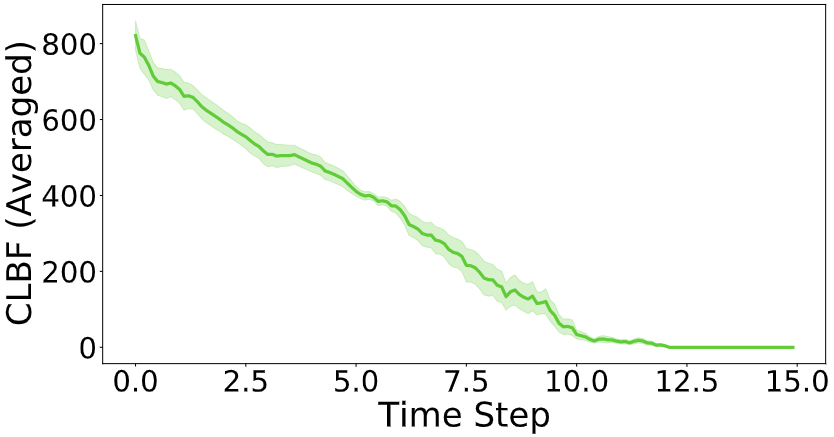
(b) The averaged changes

Figure 6: The changes in CLBF value under different initial conditions. In (a), we show the changes in CLBF value along the trajectories starting from ten different initial positions. In (b), the averaged change in CLBF value of these trails is plotted. The solid line indicates the average value and shadowed region for the 1-SD confidence interval of these trails.

V-D Sim-to-Real Transfer

In this part, we evaluate LBAC by deploying controllers learned in the simulators to the physical robot. As shown in Figure 1, a nano Crazyflie 2.0 quadrotor is used to achieve the autonomous navigation task and a motion capture system is used for state estimation in the real world. The trajectories of the Crazyflie starting from different initial positions are shown in Figures 7(b) and 7(c). The controllers trained by LBAC outperform other model-free safe RL algorithms in terms of both reachability and safety.

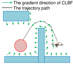
(a) Illustration of CLBF

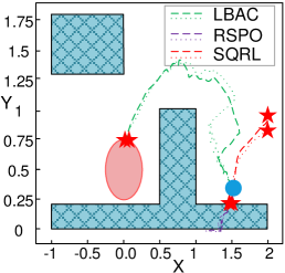
(b) Height 0.35m

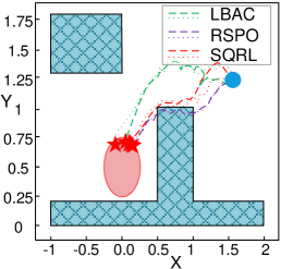
(c) Height 1.2m

Figure 7: Controllers are evaluated in real-world using a Crazyflie 2.0 quadrotor. (a) is an intuitive illustration of CLBF. In (b) and (c), the quadrotor’s initial heights are 0.35m and 1.2m. The blue circle represents the starting points, and the red stars stand for the reached positions.

VI Conclusion

In this paper, the control Lyapunov barrier function is extended to the constrained Markov decision process, and a data-based theorem is proposed to analyze closed-loop reachability and safety. Based on the theoretical results, a Lyapunov Barrier-based Actor-Critic method is proposed to search for a controller. The proposed algorithm is evaluated on a 2D quadrotor navigation task with safety constraints. Compared to existing model-free RL algorithms, the proposed method can reliably ensure reachability and safety in both simulation and real-world tests. In the future, more experiments will be conducted to validate the effectiveness and scalability of our approach. We also plan to improve the robustness of the learned controller using methods such as domain randomization and adversarial training [39].

Appendix A Proof of Lemma 1

Proof.

When $\hat{s}\in\mathcal{S}_{\overline{\text{safe}}}$, it leads to the goal state within $N$ steps. Thus, $V(\hat{s})=\underset{a\sim\pi}{\mathrm{E}}\left[\sum_{t=0}^{\infty}\gamma^{t}c(s_{t},a_{t})\mid s_{0}=\hat{s}\right]<\sum_{t=0}^{N-1}\gamma^{t}c_{\max}(s,a)=\frac{c_{\max}(s,a)\left(1-\gamma^{N}\right)}{1-\gamma}$. In order to have $V(\hat{s})<\hat{c}$, we set $\frac{c_{\max}(s,a)\left(1-\gamma^{N}\right)}{1-\gamma}<\hat{c}$. When $\hat{s}\in\mathcal{S}_{\overline{\text{unsafe}}}$, it leads to unsafe state within $N$ steps. Thus, $V(\hat{s})\geq\sum_{t=0}^{N-1}\gamma^{t}c_{\min}(s,a)+\sum_{t=N}^{\infty}\gamma^{t}C=\frac{c_{\min}(s,a)\left(1-\gamma^{N}\right)+C\gamma^{N}}{1-\gamma}$. In order to have $V(\hat{s})\geq\hat{c}$, we set $\frac{c_{\min}(s,a)\left(1-\gamma^{N}\right)+C\gamma^{N}}{1-\gamma}\geq\hat{c}$. Rearranging, we have $C\geq\frac{(1-\gamma)\hat{c}-c_{\min}(s,a)\left(1-\gamma^{N}\right)}{\gamma^{N}}$. With $c_{\min}(s,a)=0$, it is simplified to $C\geq\frac{1-\gamma}{\gamma^{N}}\hat{c}>\frac{c_{\max}(s,a)\left(1-\gamma^{N}\right)}{\gamma^{N}}$. To this end, the condition (3) is achieved. ∎

Appendix B Proof of Theorem 1

Proof.

To prove that $N$ is finite based on the conditions and assumptions where $N=\max\{t:\mathbb{P}(s\in\Delta|\rho,\pi,t)>0\}$, we will assume that $N$ is infinity and prove by contradiction. $N=\infty$ if for any $\epsilon$ there exists an instant $t>\epsilon$ such that $\mathbb{P}(s\in\Delta|\rho,\pi,t)>0$. In that case, the finite-horizon sampling distribution $\mu_{N}(s)$ turns into the infinite-horizon sampling distribution $\mu(s)=\lim_{N\rightarrow\infty}\mu_{N}(s)=\lim_{N\rightarrow\infty}\frac{1}{N}\sum_{t=1}^{N}p(s|\rho,\pi,t)$. The existence of $\mu(s)$ is guaranteed by the existence of $q_{\pi}(s)=\lim_{t\rightarrow\infty}p(s\mid\rho,\pi,t)$, which has been commonly exploited by many RL literature [34, 40]. Since the sequence $\{p(s|\rho,\pi,t),t\in\mathbb{Z}_{+}\}$ converges to $q_{\pi}(s)$ as $t$ approaches $\infty$, then by the Abelian theorem, the sequence $\{\frac{1}{T}\sum_{t=1}^{T}p(s|\rho,\pi,t),T\in\mathbb{Z}_{+}\}$ also converges and $\mu(s)=q_{\pi}(s)$. Then one naturally has that the sequence $\{\mu_{N}(s)V(s),T\in\mathbb{Z}_{+}\}$ converges pointwise to $q_{\pi}(s)V(s)$.

According to Lebesgue’s dominated convergence theorem [41], if a sequence ${f_{n}(s)}$ converges point-wise to a function $f$ and is dominated by some integrable function $g$ in the sense that,$|f_{n}(s)|\leq g(s),\forall s\in\mathcal{S},\forall n$, then one has $\lim_{n\rightarrow\infty}\int_{\mathcal{S}}f_{n}(s)\mathrm{d}s=\int_{\mathcal{S}}\lim_{n\rightarrow\infty}f_{n}(s)\mathrm{d}s$.

Applying this theorem to the left-hand side of (4)

$$\mathbb{E}_{s\sim\mu}\left(\mathbb{E}_{s^{\prime}\sim p_{\pi}}V(s^{\prime})\mathds{1}_{\Delta}(s^{\prime})-V(s)\mathds{1}_{\Delta}(s)\right)$$ (9)

$$= \int_{\mathcal{S}}\lim_{N\rightarrow\infty}\frac{1}{N}\sum_{t=1}^{N}p(s|\rho,\pi,t)(\int_{\mathcal{S}}p_{\pi}(s^{\prime}|s)V(s^{\prime})\mathds{1}_{\Delta}(s^{\prime})\mathrm{d}s^{\prime}$$

$$-V(s)\mathds{1}_{\Delta}(s))\mathrm{d}s$$

$$= \lim_{N\rightarrow\infty}\frac{1}{N}\sum_{t=1}^{N}\int_{\mathcal{S}}V(s^{\prime})\mathds{1}_{\Delta}(s^{\prime})\int_{\mathcal{S}}p_{\pi}(s^{\prime}|s)p(s|\rho,\pi,t)\mathrm{d}s\mathrm{d}s^{\prime}$$

$$- \lim_{N\rightarrow\infty}\frac{1}{N}\sum_{t=1}^{N}\int_{\mathcal{S}}p(s|\rho,\pi,t)V(s)\mathds{1}_{\Delta}(s)\mathrm{d}s$$

$$= \lim_{N\rightarrow\infty}\frac{1}{N}(\sum_{t=2}^{N+1}\mathbb{E}_{p(s|\rho,\pi,t)}V(s)\mathds{1}_{\Delta}(s)$$

$$-\sum_{t=1}^{N}\mathbb{E}_{p(s|\rho,\pi,t)}V(s)\mathds{1}_{\Delta}(s))$$

$$= \lim_{N\rightarrow\infty}\frac{1}{N}(\mathbb{E}_{p(s|\rho,\pi,N+1)}V(s)\mathds{1}_{\Delta}(s)-\mathbb{E}_{\rho(s)}V(s)\mathds{1}_{\Delta}(s))$$

Since $\mathbb{E}_{\rho(s)}V(s)$ is finite, thus the limitation value $\lim_{N\rightarrow\infty}\frac{1}{N}(\mathbb{E}_{\rho(s)}V(s)\mathds{1}_{\Delta}(s))=0$. The above equation equals to $\lim_{N\rightarrow\infty}\frac{1}{N}\mathbb{E}_{p(s|\rho,\pi,N+1)}V(s)\mathds{1}_{\Delta}(s)$. Note that $V(s)\geq\alpha_{1}c_{\pi}(s)$, $\forall s\in\mathcal{S}$, and $c_{\pi}(s)>\delta$, $\forall s\in\Delta$. Thus, $\lim_{N\rightarrow\infty}\frac{1}{N}\mathbb{E}_{p(s|\rho,\pi,N+1)}V(s)\mathds{1}_{\Delta}(s)\geq\lim_{N\rightarrow\infty}\frac{\alpha_{1}\delta}{N}\mathbb{E}_{p(s|\rho,\pi,N+1)}\mathds{1}_{\Delta}(s)=0$

Since $\mu(s)=q_{\pi}(s)$, the right-hand side of (4) equals to $-\alpha_{4}\mathbb{E}_{s\sim q_{\pi}}c_{\pi}(s)\mathds{1}_{\Delta}(s)\leq-\alpha_{4}\mathbb{E}_{s\sim q_{\pi}}\delta\mathds{1}_{\Delta}(s)=-\alpha_{4}\delta\lim_{t\rightarrow\infty}\mathbb{P}(s\in\Delta|\rho,\pi,t)$. Combining the above inequalities with (4), one has $\lim_{t\rightarrow\infty}\mathbb{P}(s\in\Delta|\rho,\pi,t)<0$, which is contradictory to the fact that $\mathbb{P}(s\in\Delta|\rho,\pi,t)$ is nonnegative. Thus there exist a finite $N$ such that $\mathbb{P}(s\in\Delta|\rho,\pi,t)=0$ for all $t>N$. In other word, the agent will reach the goal region or the unsafe region within $N$ steps. According to (3), $s_{0}\in\mathcal{S}_{\overline{\text{safe}}},V(s_{0})<\hat{c}$ where the agent will reach the goal region and avoid the unsafe region, while $s_{0}\in\mathcal{S}_{\overline{\text{unsafe}}},V(s_{0})\geq\hat{c}$ where the agent will reach the unsafe region within $N$ steps. The process of building such function $V$ is described in Section IV-A. ∎

Appendix C 2D Quadrotor Navigation

The state of the 2D quadrotor model is defined as $s=[p_{x},p_{y},v_{x},v_{y}]$, with control input $a=[v_{x_{\text{des}}},v_{y_{\text{des}}}]$. In this experiment, the controller is expected to navigate a 2D quadrotor to the goal set $\boldsymbol{S}_{\text{goal}}$ without colliding with the obstacles. We define the state space as $\mathcal{S}=\left\{\boldsymbol{s}:\boldsymbol{s}_{\mathrm{lb}}\leq\boldsymbol{s}\leq\boldsymbol{s}_{\mathrm{ub}}\right\}$ with $\boldsymbol{s}_{\mathrm{lb}}=[-1,0,-0.25,-0.25]$ and $\boldsymbol{s}_{\mathrm{ub}}=[2,1.8,0.25,0.25]$, representing the lower bound and upper bound of the set of the valid states. The action space is set as $\mathcal{A}=\left\{\boldsymbol{a}:-\boldsymbol{a}_{\mathrm{b}}\leq\boldsymbol{a}\leq\boldsymbol{a}_{\mathrm{b}}\right\}$ with $\boldsymbol{a}_{\mathrm{b}}=[0.25,0.25]$, by considering the real world hardware limitation. The cost function is designed as $c=\sqrt{4p_{x}^{2}+(p_{y}-0.5)^{2}}$. We set the obstacle set $\mathcal{S}_{o1}=\left\{\boldsymbol{s}:0.5\leq p_{x}\leq 1,0.2\leq p_{y}\leq 1\right\}$, $\mathcal{S}_{o2}=\left\{\boldsymbol{s}:-1\leq p_{x}\leq 0,1.3\leq p_{y}\leq 1.8\right\}$ and $\mathcal{S}_{o3}=\left\{\boldsymbol{s}:p_{z}\leq 0.2\right\}$, the unsafe state set $\mathcal{S}_{\text{unsafe}}=\left\{\boldsymbol{s}:\mathcal{S}_{o1}\cup\mathcal{S}_{o2}\cup\mathcal{S}_{o3}\right\}$, the goal state set $\mathcal{S}_{\text{goal}}=\left\{\boldsymbol{s}:\sqrt{p_{x}^{2}+(p_{y}-0.5)^{2}}\leq 0.3\right\}$. Once the quadrotor reaches the $\mathcal{S}_{\text{unsafe}}$, the episode ends in advance and the cost function is set as $C=2000$. The episodes are of maximum length 200 and time step $dt=0.1$ s. In the experiments, we use Bitcraze’s Crazyflie 2.0 quadrotors. We train the controllers in the simulator gym-pybullet-drones [42] based on PyBullet. In the real world, we use a motion capture system for state estimation.

Appendix D Hyperparameter setting

For LBAC, there are two networks: the controller network (actor) and the control Lyapunov barrier network (critic). The controller network is represented by a fully-connected neural network with two hidden layers of size 256 each, with the ReLU activation function, outputting the mean and standard deviations of a Gaussian distribution. A fully-connected neural network represents the control Lyapunov barrier critic network with two hidden layers of size 256, each with a ReLU activation function. We use the vanilla Soft Actor-Critic algorithm [36] for 500 episodes to explore the environment effectively as a warm start. The hyperparameters can be found in Table I

TABLE I: Hyperparameter setting in LBAC

Hyperparameters	2D Quadrotor Navigation
Minibatch size	512
Total episode	2500
Actor learning rate	$3\times 10^{-4}$
Critic learning rate	$3\times 10^{-4}$
Terminal cost $C$	2000
Discount factor $\gamma$	0.999

In RSPO and SQRL, another safety critic network $Q_{\text{risk}}$ is needed to estimate the discounted future probability of constraint violation with discounted $\gamma_{\text{risk}}$. The safety threshold $\varepsilon_{\text{risk }}\in[0,1]$ is an upper-bound on the expected risk of the action. In this paper, the safety critic network shares the same architecture as the task critic network, except that a sigmoid activation is added to the output layer to ensure that the outputs are on $[0,1]$. We use the same hyperparameter settings as LBAC in RSPO, RCPO, and SQRL. The other hyperparameters can be found in Table II.

TABLE II: Hyperparameter setting in safe RL

Hyperparameters	2D Quadrotor Navigation
RCPO $\left(\gamma_{\text{risk }},\lambda\right)$	$\left(0.99,3000\right)$
RSPO $\left(\gamma_{\text{risk }},\varepsilon_{\text{risk }},\lambda\right)$	$\left(0.99,0.2,10000\right)$
SQRL $\left(\gamma_{\text{risk }},\varepsilon_{\text{risk }},\lambda\right)$	$\left(0.99,0.2,5000\right)$

References

- [1] A. Nagabandi, K. Konolige, S. Levine, and V. Kumar, “Deep dynamics models for learning dexterous manipulation,” in Conference on Robot Learning. PMLR, 2020, pp. 1101–1112.
- [2] G. Kahn, A. Villaflor, V. Pong, P. Abbeel, and S. Levine, “Uncertainty-aware reinforcement learning for collision avoidance,” arXiv preprint arXiv:1702.01182, 2017.
- [3] N. O. Lambert, D. S. Drew, J. Yaconelli, S. Levine, R. Calandra, and K. S. Pister, “Low-level control of a quadrotor with deep model-based reinforcement learning,” IEEE Robotics and Automation Letters, vol. 4, no. 4, pp. 4224–4230, 2019.
- [4] S. Belkhale, R. Li, G. Kahn, R. McAllister, R. Calandra, and S. Levine, “Model-based meta-reinforcement learning for flight with suspended payloads,” IEEE Robotics and Automation Letters, vol. 6, no. 2, pp. 1471–1478, 2021.
- [5] J. Achiam, D. Held, A. Tamar, and P. Abbeel, “Constrained policy optimization,” in International conference on machine learning. PMLR, 2017, pp. 22–31.
- [6] G. Thomas, Y. Luo, and T. Ma, “Safe reinforcement learning by imagining the near future,” Advances in Neural Information Processing Systems, vol. 34, 2021.
- [7] C. Tessler, D. J. Mankowitz, and S. Mannor, “Reward constrained policy optimization,” arXiv preprint arXiv:1805.11074, 2018.
- [8] R. Cheng, G. Orosz, R. M. Murray, and J. W. Burdick, “End-to-end safe reinforcement learning through barrier functions for safety-critical continuous control tasks,” in Proceedings of the AAAI Conference on Artificial Intelligence, vol. 33, no. 01, 2019, pp. 3387–3395.
- [9] T.-H. Pham, G. De Magistris, and R. Tachibana, “Optlayer-practical constrained optimization for deep reinforcement learning in the real world,” in 2018 IEEE International Conference on Robotics and Automation (ICRA). IEEE, 2018, pp. 6236–6243.
- [10] M. Ohnishi, L. Wang, G. Notomista, and M. Egerstedt, “Barrier-certified adaptive reinforcement learning with applications to brushbot navigation,” IEEE Transactions on robotics, vol. 35, no. 5, pp. 1186–1205, 2019.
- [11] K. Srinivasan, B. Eysenbach, S. Ha, J. Tan, and C. Finn, “Learning to be safe: Deep rl with a safety critic,” arXiv preprint arXiv:2010.14603, 2020.
- [12] Y. Shen, M. J. Tobia, T. Sommer, and K. Obermayer, “Risk-sensitive reinforcement learning,” Neural computation, vol. 26, no. 7, pp. 1298–1328, 2014.
- [13] A. J. Taylor, V. D. Dorobantu, H. M. Le, Y. Yue, and A. D. Ames, “Episodic learning with control lyapunov functions for uncertain robotic systems,” in 2019 IEEE/RSJ International Conference on Intelligent Robots and Systems (IROS). IEEE, 2019, pp. 6878–6884.
- [14] R. Grandia, A. J. Taylor, A. D. Ames, and M. Hutter, “Multi-layered safety for legged robots via control barrier functions and model predictive control,” in 2021 IEEE International Conference on Robotics and Automation (ICRA), 2021, pp. 8352–8358.
- [15] Q. Nguyen, A. Hereid, J. W. Grizzle, A. D. Ames, and K. Sreenath, “3d dynamic walking on stepping stones with control barrier functions,” in 2016 IEEE 55th Conference on Decision and Control (CDC), 2016, pp. 827–834.
- [16] T. Gurriet, A. Singletary, J. Reher, L. Ciarletta, E. Feron, and A. Ames, “Towards a framework for realizable safety critical control through active set invariance,” in 2018 ACM/IEEE 9th International Conference on Cyber-Physical Systems (ICCPS). IEEE, 2018, pp. 98–106.
- [17] P. Jagtap, G. J. Pappas, and M. Zamani, “Control barrier functions for unknown nonlinear systems using gaussian processes,” in 2020 59th IEEE Conference on Decision and Control (CDC), 2020, pp. 3699–3704.
- [18] J. Choi, F. Castañeda, C. J. Tomlin, and K. Sreenath, “Reinforcement learning for safety-critical control under model uncertainty, using control lyapunov functions and control barrier functions,” in Robotics: Science and Systems (RSS), 2020.
- [19] C. Dawson, Z. Qin, S. Gao, and C. Fan, “Safe nonlinear control using robust neural lyapunov-barrier functions,” in Conference on Robot Learning. PMLR, 2022, pp. 1724–1735.
- [20] Y. Meng, Y. Li, M. Fitzsimmons, and J. Liu, “Smooth converse lyapunov-barrier theorems for asymptotic stability with safety constraints and reach-avoid-stay specifications,” Automatica, vol. 144, p. 110478, 2022.
- [21] W. Jin, Z. Wang, Z. Yang, and S. Mou, “Neural certificates for safe control policies,” arXiv preprint arXiv:2006.08465, 2020.
- [22] M. Z. Romdlony and B. Jayawardhana, “Stabilization with guaranteed safety using control lyapunov–barrier function,” Automatica, vol. 66, pp. 39–47, 2016.
- [23] P. Geibel and F. Wysotzki, “Risk-sensitive reinforcement learning applied to control under constraints,” Journal of Artificial Intelligence Research, vol. 24, pp. 81–108, 2005.
- [24] A. Tamar, Y. Glassner, and S. Mannor, “Policy gradients beyond expectations: Conditional value-at-risk,” arXiv preprint arXiv:1404.3862, 2014.
- [25] F. Berkenkamp, M. Turchetta, A. Schoellig, and A. Krause, “Safe model-based reinforcement learning with stability guarantees,” Advances in neural information processing systems, vol. 30, 2017.
- [26] M. Turchetta, F. Berkenkamp, and A. Krause, “Safe exploration in finite markov decision processes with gaussian processes,” Advances in Neural Information Processing Systems, vol. 29, 2016.
- [27] B. Thananjeyan, A. Balakrishna, S. Nair, M. Luo, K. Srinivasan, M. Hwang, J. E. Gonzalez, J. Ibarz, C. Finn, and K. Goldberg, “Recovery rl: Safe reinforcement learning with learned recovery zones,” IEEE Robotics and Automation Letters, vol. 6, no. 3, pp. 4915–4922, 2021.
- [28] H. Bharadhwaj, A. Kumar, N. Rhinehart, S. Levine, F. Shkurti, and A. Garg, “Conservative safety critics for exploration,” arXiv preprint arXiv:2010.14497, 2020.
- [29] Y. Chow, O. Nachum, E. Duenez-Guzman, and M. Ghavamzadeh, “A lyapunov-based approach to safe reinforcement learning,” Advances in neural information processing systems, vol. 31, 2018.
- [30] Y. Chow, O. Nachum, A. Faust, E. Duenez-Guzman, and M. Ghavamzadeh, “Lyapunov-based safe policy optimization for continuous control,” arXiv preprint arXiv:1901.10031, 2019.
- [31] E. Altman, Constrained Markov decision processes: stochastic modeling. Routledge, 1999.
- [32] A. Agrawal and K. Sreenath, “Discrete control barrier functions for safety-critical control of discrete systems with application to bipedal robot navigation.” in Robotics: Science and Systems, vol. 13. Cambridge, MA, USA, 2017.
- [33] Z.-P. Jiang, T. Bian, W. Gao et al., “Learning-based control: A tutorial and some recent results,” Foundations and Trends® in Systems and Control, vol. 8, no. 3, pp. 176–284, 2020.
- [34] M. Han, L. Zhang, J. Wang, and W. Pan, “Actor-critic reinforcement learning for control with stability guarantee,” IEEE Robotics and Automation Letters, vol. 5, no. 4, pp. 6217–6224, 2020.
- [35] T. P. Lillicrap, J. J. Hunt, A. Pritzel, N. Heess, T. Erez, Y. Tassa, D. Silver, and D. Wierstra, “Continuous control with deep reinforcement learning,” arXiv preprint arXiv:1509.02971, 2015.
- [36] T. Haarnoja, A. Zhou, P. Abbeel, and S. Levine, “Soft actor-critic: Off-policy maximum entropy deep reinforcement learning with a stochastic actor,” in International conference on machine learning. PMLR, 2018, pp. 1861–1870.
- [37] D. P. Bertsekas, “Nonlinear programming,” Journal of the Operational Research Society, vol. 48, no. 3, pp. 334–334, 1997.
- [38] A. D. Ames, J. W. Grizzle, and P. Tabuada, “Control barrier function based quadratic programs with application to adaptive cruise control,” in 53rd IEEE Conference on Decision and Control. IEEE, 2014, pp. 6271–6278.
- [39] L. Brunke, M. Greeff, A. W. Hall, Z. Yuan, S. Zhou, J. Panerati, and A. P. Schoellig, “Safe learning in robotics: From learning-based control to safe reinforcement learning,” Annual Review of Control, Robotics, and Autonomous Systems, vol. 5, 2021.
- [40] M. Han, Y. Tian, L. Zhang, J. Wang, and W. Pan, “Reinforcement learning control of constrained dynamic systems with uniformly ultimate boundedness stability guarantee,” Automatica, vol. 129, p. 109689, 2021.
- [41] H. L. Royden and P. Fitzpatrick, Real analysis. Macmillan New York, 1988, vol. 32.
- [42] J. Panerati, H. Zheng, S. Zhou, J. Xu, A. Prorok, and A. P. Schoellig, “Learning to fly—a gym environment with pybullet physics for reinforcement learning of multi-agent quadcopter control,” in 2021 IEEE/RSJ International Conference on Intelligent Robots and Systems (IROS), 2021.