Score Operator Newton Transport

Abstract

We propose a new approach for sampling and Bayesian computation that uses the score of the target distribution to construct a transport from a given reference distribution to the target. Our approach is an infinite-dimensional Newton method, involving an elliptic PDE, for finding a zero of a “score-residual” operator. We use classical elliptic PDE theory to prove convergence to a valid transport map. Our Newton iterates can be computed by exploiting fast solvers for elliptic PDEs, resulting in new algorithms for Bayesian inference and other sampling tasks. We identify elementary settings where score-operator Newton transport achieves fast convergence while avoiding mode collapse.

1 Introduction

Generating samples from a complex (e.g., non-Gaussian, high-dimensional) probability distribution is a core computational challenge in diverse applications, ranging from computational statistics and machine learning to molecular simulation. A recurring setting is where the density $\rho$ of the target distribution is specified up to a normalizing constant—for example, in Bayesian modeling, where $\rho$ represents the posterior density. Here, evaluations of the score $\nabla\log\rho$ are often available as well, even for complex statistical models [Villa et al., 2021]. Alternatively, many new methods enable effective score estimation from data, without explicit density estimation; examples include score estimation from time series observations in chaotic dynamical systems [Chandramoorthy and Wang, 2022, Ni, 2020] and score-based modeling of image distributions [Song et al., 2020b, a].

In these settings, transport or “flow”-driven algorithms for generating samples have seen extensive success. The central idea is to construct a transport map from a simple, prescribed source distribution to the target distribution of interest. One class of transport approaches, e.g., as represented by variational inference with normalizing flows, involves constructing a parametric class of invertible maps and minimizing some statistical divergence between the pushforward (see Section 2) of the source by a member of this class and the target. A different, essentially nonparametric, class of transport approaches are based on particle systems, e.g., Stein variational gradient descent (SVGD) [Liu and Wang, 2016] and its many variants [Li et al., 2020a, Chen and Ghattas, 2020, Detommaso et al., 2018]. These methods can be interpreted as gradient flows [Jordan et al., 1998] of some functional on the space of probability measures, for different choices of geometry [Chewi et al., 2020, Duncan et al., 2019]. Such methods yield implicit representations of transport maps, through the paths taken by sample trajectories [Han and Liu, 2017]. Yet another class of transport methods involve prescribing continuous paths [Masrani et al., 2021, Albergo et al., 2023] between the source and target distributions, and approximating these paths with particle systems or learned velocity fields.

Of course, none of these approaches is without drawbacks. Parametric representations of transport maps often involve ad hoc choices of parametric class, where bias must be balanced against complexity of the representation; moreover, the optimization problems that must be solved over such classes seldom have guarantees. On the other hand, gradient flow approaches, as exemplified by SVGD or more generally standard Langevin dynamics, may be slow to converge and quite sensitive to the geometry and dimensionality of the target distribution. Because the transport map is not explicitly available in these approaches, it is generally difficult to update the map, e.g., for perturbed scores, or to reuse the map for downstream computations. Continuous-time “homotopy” approaches require a priori selection of a path through the space of probability measures, and may involve solving equations that depend explicitly on estimates of the density at the current time [Reich, 2011] or otherwise resorting to cruder approximations [Iglesias and Yang, 2021].

This paper introduces a new sampling approach based on different ingredients: an infinite-dimensional score matching principle and discrete-time dynamics. Specifically, we construct a transport map as the zero of a score residual operator via an infinite-dimensional Newton method for root finding, which is typically called the Newton–Raphson method in finite dimensions. The transport is a composition of maps found, at each step, via solution of a linear elliptic partial differential equation (PDE). We harness regularity theory for elliptic PDEs to prove existence of such a map and to prove convergence of the iterations. The resulting score-operator Newton (SCONE) transport construction is illustrated in Figure 1. It applies to any sampling problem where the scores of the source and target measures can be evaluated. Several desirable features of our approach are as follows:

• Newton methods are efficient: we will show, empirically and in simple analytical examples (see Appendix C), that very few iterations may be required. The Newton construction also permits an existing map to be updated or fine-tuned, e.g., for perturbed scores; this is useful for applications such as Bayesian filtering.

• Unlike the nonlinear Monge-Ampère equation, which describes optimal transport maps, our construction involves a sequence of linear PDEs, which are more amenable to analysis, fast computation, and dimension reduction.

• Elliptic differential operators instantaneously propagate information throughout the domain. Hence, our transport updates, which are elliptic PDE solutions, are intrinsically global [Evans, 2022]. As evidenced by our numerical results, our construction thus tends to avoid mode collapse, since transport updates are influenced by score values over the entire support of the distributions, including the tails.

We summarize our main contributions as follows: We define a score transformation operator that maps an input score and a transport map to the transported score. We prove the existence of transport maps that are fixed points of an operator based on the score-transformation operator and the target score. Our existence proof is constructive and leads to a Newton method on Banach spaces. Our construction yields a transport map and defines a new notion of score-matching in infinite dimensions. Convergence of transport maps, and scores, is established in classical Hölder norms, unlike in dual norms typically used for variational inference methods.

In this paper, we establish the theoretical foundations of score operator Newton transport and provide proof-of-concept numerics. Our construction and theory are developed in the infinite-dimensional setting, enabling flexible representations of the transport map. Hence, the construction facilitates the development of many new sampling algorithms, based on kernel methods, deep neural networks, and other discretizations of the underlying linear elliptic PDEs. Developing such scalable algorithms for the Newton updates will be a subject of our future work.

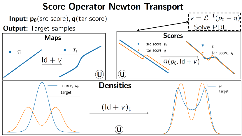
Figure 1: A graphical overview of the construction of transport maps. The score of the source and target densities are given as inputs. The method outputs samples from the target distribution. Each iteration involves solving an elliptic PDE that gradually transports the score of the source to that of the target. The PDE solutions across iterations are combined via a simple composition operation to obtain the transport map from the source to the target.

2 Infinite-dimensional score matching

Suppose $\nu$ is our unknown target probability measure on $\mathbb{R}^{d}$ with associated density $\rho^{\nu}.$ We define the score of the target to be the vector-valued function $q:=\nabla\log\rho^{\nu}:\mathbb{R}^{d}\to\mathbb{R}^{d}.$ In our setting, the target score $q(x)$ is available at every $x\in\mathbb{R}^{d}.$

Let $\mu$ be a source or reference probability measure on $\mathbb{R}^{d}$ with density $\rho^{\mu}$. The source is chosen to be easy to sample from, e.g., a Gaussian in $\mathbb{R}^{d}$. Its vector-valued score function is defined as $p:=\nabla\log\rho^{\mu}.$ Here $\nabla$ is the gradient operator on Euclidean space. The main contribution of this work is a new transport map to sample from the target $\nu$ using the source samples from $\mu$ and the source and target scores,

$$p(x):=\nabla\log\rho^{\mu}(x),\quad q(x):=\nabla\log\rho^{\nu}(x).$$

Our transport map is defined as the solution of an infinite-dimensional root finding problem for the score operator. Next we define both these objects: transport maps and the score operator.

Transport maps: Given two probability measures $\mu$ and $\nu$ on $\mathbb{R}^{d}$, we say that a measurable function $T:\mathbb{R}^{d}\to\mathbb{R}^{d}$ is a transport map from $\mu$ to $\nu$ if

$$\nu(A)=(T_{\sharp}\mu)(A)\coloneqq\mu(T^{-1}(A)),$$ (1)

for every measurable set $A$; here $\sharp$ denotes the pushforward operation. In high-dimensional inference problems, the target $\nu$ that we wish to sample from is a often a complicated “intractable” measure. Our goal is to find an invertible map $T$ that transforms samples of $\mu$ to samples distributed according to $\nu$. Recall that samples from the source $\mu$ are easily obtained.

In general, the transport map $T$ between the source and target measures is not unique. The optimal transport map is one useful and canonical choice, but in the context of Bayesian inference—where our main goal is to simulate $\nu$—it suffices to find any transport $T$ that is computationally feasible. Now we provide a constructive approximation of a map $T$ that satisfies (1) by exploiting the scores, $p=\nabla\log\rho^{\mu}$ and $q=\nabla\log\rho^{\nu}$, associated with the source $\mu$ and target $\nu$, respectively. To do this, we define a score operator on the product space of functions representing scores and transport maps.

Score operator: We define a score operator, denoted by $\mathcal{G}$, that takes as arguments a source score and an invertible transport map and returns the score of the resulting pushforward distribution. That is, if $T$ is an invertible map such that $T_{\sharp}\mu=\nu$, the operator $\mathcal{G}$ is defined such that

$$\mathcal{G}(p,T)=q.$$ (2)

Recall the change of variables formula for probability densities,

$$\rho^{\nu}=\dfrac{\rho^{\mu}\circ T^{-1}}{|{\rm det}\nabla T|\circ T^{-1}}.$$ (3)

Taking logarithms and differentiating the above formula, we obtain a definition for the score operator $\mathcal{G}$,

$$\mathcal{G}(s,U) =\left(s(\nabla U)^{-1}-\nabla\log|{\rm det}\nabla U|(\nabla U)^{-1}\right)\circ U^{-1}$$ (4)

$$=\Big{(}s\,(\nabla U)^{-1}-{\rm tr}\big{(}(\nabla U)^{-1}\nabla^{2}U\big{)}(\nabla U)^{-1}\Big{)}\circ U^{-1},$$ (5)

where (5) follows from using Jacobi’s formula for the derivative of the determinant. We use ${\rm tr}((\nabla U)^{-1}\nabla^{2}U)$ for the vector-valued function $[{\rm tr}((\nabla U)^{-1}\partial_{1}\nabla U),\ldots,{\rm tr}((\nabla U)^{-1}\partial_{d}\nabla U)]^{\top}$, where $\partial_{i}$ is the partial derivative in the $i$th coordinate. The above operator takes as arguments a score $s$ associated with a probability measure, say $\pi$, and a $\mathcal{C}^{2}$-diffeomorphism $U$, to return the score associated with the measure $U_{\sharp}\pi$. That is, $\mathcal{G}$ expresses the change of variables, or the pushforward operation, on the space of scores. We end this section by listing some properties of $\mathcal{G}$ that will be useful in the sections to follow and can be checked by using the above definitions.

1. $\mathcal{G}(s,{\rm Id})=s$ for any score $s$, expressing the fact that the identity coupling results in the same probability measure;

2. $\mathcal{G}(s,{\rm Id}+c)=s\circ({\rm Id}-c)$, where $c$ is a constant function;

3. $\mathcal{G}$ has the group property, mimicking the pushforward operator. That is,

   $$\mathcal{G}(s,\psi_{1}\circ\psi_{2})=\mathcal{G}(\mathcal{G}(s,\psi_{2}),\psi_{1}).$$

Note that the operator $\mathcal{G}$ is not injective in the second argument, and hence not invertible. That is, $\mathcal{G}(s,U_{1})=\mathcal{G}(s,U_{2})$ does not imply that $U_{1}=U_{2}$. Any solution $T$ to (2) is a valid transport map from $\mu$ to $\nu$. We refer to the problem of finding a $T$ that satisfies (2) as the infinite-dimensional score-matching problem. This is because the solution $T$ is a function, and the score of the pushforward distribution through $T$ matches the target score $q.$ Despite its name, our problem is not derived as an infinite-dimensional version of the score-matching problem from [Hyvärinen and Dayan, 2005], which is essentially a density estimation problem. Here our objective is to obtain a transport map given target scores and to use it for sampling. In the next section, we will define a score-residual operator that maps a score and a transport map to the difference between the target score and the score of the pushforward of the source by the transport map. We will then derive a solution to the score-matching problem as a zero of this operator; thus, our solution strategy for transport also deviates from the variational problem involving the typical score-matching objective in the literature [Hyvärinen and Dayan, 2005, Song and Ermon, 2019, Song et al., 2020b, Wibisono and Yang, 2022].

Remark 1 (Availability of scores).

As mentioned in the introduction, the target score is available in settings beyond Bayesian inference with a tractable likelihood and prior. In other words, in many settings, scores can be approximated well even though an explicit model for the unnormalized density is not available. One such example is the score of an ergodic, invariant measure of certain classes of chaotic systems. Here, fast methods have been developed to evaluate scores at any point on a chaotic orbit [Chandramoorthy and Wang, 2022, Ni, 2020].

Remark 2 (Validity of transport maps).

Note that any diffeomorphism that satisfies $\mathcal{G}(p,T)=q$ is a valid transport map in the sense that $T_{\sharp}\mu=\nu$. By integrating both sides of (5), we obtain that any $T$ that satisfies $\mathcal{G}(p,T)=q$ also satisfies, $\rho^{\nu}=k\rho^{\mu}\circ T^{-1}/|{\rm det}\nabla T|$, for an integration constant $k.$ Since the left hand side is a valid density (integrates to 1), we obtain that $k$ must be 1.

3 Learning a zero of the score-residual operator

Fixing $p$ and $q$, we define the score-residual operator on the space of $\mathcal{C}^{2}$-diffeomorphisms on $\mathbb{R}^{d}$ as

$$\mathcal{R}(T)\coloneqq\mathcal{G}(p,T)-q.$$

A zero of this operator is a transport map between the measures associated with $p$ and $q$. Here we describe an iterative approach for finding a zero of this operator, which is a generalization of Newton’s method to infinite-dimensional spaces.

3.1 Score operator Newton (SCONE) method

Infinite-dimensional generalizations of the Newton method appear in the analysis of PDEs under the name of Nash–Moser iteration [Berti and Bolle, 2015]. They also appear in the context of finding conjugacies between nearby dynamical systems, in an approach called the Kolmogorov–Arnold–Moser or KAM method [Moser, 1961]. In the next section, we derive sufficient conditions for the convergence of this method.

To develop the SCONE iteration, we expand the score operator, supposing that $p$ is close to $q$ and assuming a linear structure on function space near $(q,{\rm Id})$,

$$\mathcal{G}(p,T) =\mathcal{G}(q,{\rm Id})+D_{1}\mathcal{G}(q,{\rm Id})(p-q)+$$ (6)

$$D_{2}\mathcal{G}(q,{\rm Id})(T-{\rm Id})+\Delta(p,T),$$

where ${\rm Id}$ is the identity function on $\mathbb{R}^{d}$, $D_{1},D_{2}$ are first-order partial derivatives (Frechét derivatives) of $\mathcal{G}$ in its first and second arguments respectively, and $\Delta(p,T)$ contains nonlinear operators on $p-q$ and $T-{\rm Id}$. Analogous to the elementary Newton method, to find the solution to the score-matching problem, we first look for a solution to the linearized score-matching problem. That is, we find such a $T$ for which the left hand side of (6) is $q$ and $\Delta(p,T)=0$. This linearization of the score-matching problem yields,

$$-D_{1}\mathcal{G}(q,{\rm Id})\>(p-q)=D_{2}\mathcal{G}(q,{\rm Id})v,$$ (7)

defining the vector field

$$v\coloneqq T-{\rm Id}.$$

Since $\mathcal{G}(p,{\rm Id})=p$ for all $p$, we have that $D_{1}\mathcal{G}(q,{\rm Id})={\rm Id}$. We can explicitly compute the linear operator $D_{2}\mathcal{G}(q,{\rm Id})$ to be the following differential operator, which, for convenience, we define as $\mathcal{L}(q)$,

$$-D_{2}\mathcal{G}(q,{\rm Id})\>v=\mathcal{L}(q)\>v:=\nabla q\>v+q\>\nabla v+{\rm tr}(\nabla^{2}v).$$ (8)

In the above, the trace ${\rm tr}(\nabla^{2}v)$ of the tensor $\nabla^{2}v$ is a row vector with the $i$th column being ${\rm tr}(\partial_{i}\nabla v)$. Using this, we obtain that $v$ satisfies,

$$(p-q)=\mathcal{L}(q)\>v.$$ (9)

We may then iterate this update in the following way. Assuming that $\mathcal{L}(q)$ is invertible, we obtain the solution $v=(\mathcal{L}(q))^{-1}(p-q)$. Using $T={\rm Id}+v$, we obtain $p_{1}=\mathcal{G}(p,T)$, and then, we repeat the update (9) with $p_{1}$ replacing $p$, and solve for $v_{1}$. We then update the transport map approximation as $T_{1}=({\rm Id}+v_{1})\circ({\rm Id}+v)$. Proceeding further, at the $n$th iteration, we obtain the function $v_{n}$ by solving

$$-(q-p_{n})=\mathcal{L}(q)v_{n}=(\nabla q)v_{n}+q_{n}(\nabla v_{n})+{\rm tr}(\nabla^{2}v_{n}).$$ (10)

Then, we set,

$$T_{n+1} \leftarrow({\rm Id}+v_{n})\circ T_{n}$$

$$p_{n+1} \leftarrow\mathcal{G}(p_{n},{\rm Id}+v_{n}).$$ (11)

In the same spirit as the KAM method from the dynamical systems literature, notice that the differential operator $\mathcal{L}(q)$ remains the same across steps, (10). In the next section, we will give sufficient conditions under which the sequence of functions $(T_{n})_{n\geq 0}$ converges, in a classical Hölder norm, to a transport map $T$, i.e., an invertible map that satisfies $T_{\sharp}\mu=\nu$.

Algorithm 1 Score-operator Newton Transport

$T_{0}(x)=x,$ $p_{0}(x)=\nabla\log\rho^{\mu}(x),$ $x_{1},x_{2},\cdots,x_{m}\sim\mu$

while $n\leq n_{\rm max}$ do

     $v_{n}\leftarrow\mathcal{L}(q)^{-1}(p_{n}-q)$

     $x_{i}\leftarrow x_{i}+v_{n}(x_{i})$

     $p_{n+1}(x)\leftarrow\mathcal{G}(p_{n},{\rm Id}+v_{n})(x)$

     $n\to n+1$

end while

Return $\{x_{i}\}_{1\leq i\leq m}$

3.2 SCONE transport algorithm

The steps of the infinite-dimensional Newton algorithm derived above are summarized in Algorithm 1. The input to the algorithm are black-box functions that return the source score $p_{0}=p$ and $q$, the target score. In addition, we have $m$ iid samples from the source distribution, say, $\{x_{i}\}_{i=1}^{m}.$ After $n$ steps of the algorithm, these samples are transformed to $\{T_{n}(x_{i})\}_{i=1}^{m},$ which represent target samples more accurately as $n$ increases. The algorithm can also return the transport map $T$ as a black-box function that can be evaluated at any point.

In the beginning, we set the initial guess for the transport map $T_{0}$ (e.g., $T_{0}(x)={\rm Id}(x)=x$) and $p_{0}=p$, the source score. At each iteration, we solve the PDE (10) to obtain the vector field $v_{n}$. There is extensive literature on approximating solutions of elliptic PDEs using neural networks, such as physics-informed neural networks [Raissi et al., 2019], deep Ritz methods [Lu et al., 2021b, Yu et al., 2018] and Fourier neural operators [Li et al., 2020b]; as well as kernel methods and Gaussian process approximations [Owhadi and Scovel, 2019, Wendland, 2004, Schaback and Wendland, 2006, Zhang et al., 2000], and finite elements [Ciarlet, 2002, Wang and Ye, 2013]. Bespoke methods that exploit the particular structure of $\mathcal{L}(q)$ are deferred to future work (see Section 6).

Using meshfree methods such as PINNs or FNOs, we obtain a black-box solution $v_{n}$ that can be evaluated at any point. Moreover, these black-box solutions, being neural networks, can also be automatically differentiated. Thus, we can evaluate $v_{n}(x_{i}),\nabla v_{n}(x_{i})$ and $\nabla^{2}v_{n}(x_{i})$, where $\{x_{i}\}_{i=1}^{m}$ are the samples at the $n$th iteration. When we use grid-based methods, we obtain (approximate) evaluations of $v_{n}$ at the grid points. Then, we use interpolations and finite-differences to obtain $v_{n}(x_{i})$ and its derivatives. Using (5), we update the source score $p_{n}$ as $p_{n+1}=\mathcal{G}(p_{n},{\rm Id}+v_{n}).$ The samples are also transformed as $x_{i}\to x_{i}+v_{n}(x_{i})$. Note that this results, at the end of the $n$th iteration, in the samples $\{T_{n}(x_{i})\},$ where $T_{n}:=({\rm Id}+v_{n})\circ T_{n-1}.$ We repeat this process until the algorithm converges, i.e., $\|v_{n}\|$ is close to zero or if the maximum number of iterations is reached.

SCONE complexity: The computational cost of our method is ${\cal O}(n\>(C_{\rm pde}+C_{\rm u}))$, where $n$ is the number of Newton iterations, $C_{\rm pde}$ is the cost of the solving the PDE and $C_{\rm u}$ is the cost of the update step (11). Typically Newton methods exhibit quadratic convergence [Galántai, 2000], which can be accelerated further for finite-dimensional problems under local smoothness conditions [Gerlach, 1994] (see Section 6). The cost of solving the PDE dominates the per iteration cost and naïve methods typically have a computational complexity that scales exponentially with the problem dimension ($d$). However, in the context of elliptic PDEs, various sparse structures in the solution have been exploited to mitigate the curse of dimensionality, including tensor decompositions [Dahmen et al., 2016], hierarchical low-rank approximations [Boullé and Townsend, 2023], and other notions of model reduction (see Section 6).

3.3 Related work

In many variational methods for sampling and Bayesian inference, one seeks transport maps that minimize a divergence or distance functional on a space of probability measures, over a parametric class of maps $\mathcal{U}$. As an example, one could define a score-based distance metric, and seek a $T$ such that

$$T=\arg\,\min_{U\in\mathcal{U}}\int\|q(x)-\mathcal{G}(p,U)(x)\|^{2}\>d\nu(x).$$ (12)

Candidate maps $U\in\mathcal{U}$ are parameterized and an empirical minimization problem for the parameters is solved using a method that is appropriate for the distance functional. Common classes of parametric maps include normalizing flows [Papamakarios et al., 2021], the flows of neural ODEs [Chen et al., 2018], and gradients of input-convex neural networks [Huang et al., 2020]. An alternative class of approaches produces implicit representations of transport maps through paths taken by sample trajectories of a deterministic or stochastic dynamics. Beginning with the classical work of Jordan et al. [1998], these dynamics are derived such that their mean field limits are gradient flows of the distance functional on the space of probability measures, for appropriate choices of objective and geometry [Chewi et al., 2020, Duncan et al., 2019, Han and Liu, 2017]. Methods that fall into this class include SVGD and Langevin dynamics. (See Wibisono [2018] for an overview of the connection between sampling methods and optimization of distance functionals on probability spaces.)

Variational autoencoders [Kingma et al., 2019] or GANs [Goodfellow et al., 2020] also transport a low-dimensional source measure to a target, learning parameterized decoders or generators by minimizing a variety of objectives. These methods have no obvious dynamical interpretation; their stable training and obtaining theoretical guarantees are challenging.

The SCONE method exploits scores but does not make use of parametric spaces to define transport maps. Rather than minimizing a distance functional, we derive a generalized Newton–Raphson method on Banach spaces to construct a zero of the operator $\mathcal{R}(T)$. This approach explicitly specifies the transport map as a composition of functions that is achieved in the limit of a discrete-time dynamical system—as opposed to a continuous-time flow—on function spaces. Our SCONE transport defines, correspondingly, a discrete-time dynamical system on the space of probability densities, with the target being a fixed point.

4 Convergence proof

Here we prove the convergence of the SCONE algorithm in 1, establishing a new construction of a transport map. We do not compute explicit bounds on the error norms, $\|p_{n}-q\|$. We invoke elliptic regularity theory to establish convergence. Our Newton iterates (10) are solutions of second-order linear, elliptic systems of PDEs, as we describe below. The operator $\mathcal{L}$ is a non-self-adjoint elliptic differential operator. Let $M$ be a compact subset of $\mathbb{R}^{d}$ and $\Omega$ be an open set containing $M$. At each step, we solve $d$ second-order PDEs of the following form,

$$\left(L(x,D)v\right)_{i}=f_{i},\;1\leq i\leq d,$$ (13)

where the linear differential operator $L$ is given by the $d\times d$ matrix with

$$L(x,D)_{ij}=\sum_{|\alpha|\leq 2}a_{\alpha}^{ij}(x)\>D^{\alpha}.$$

Here, $\alpha=(\alpha_{1},\cdots,\alpha_{d})$ is a multi-index, $D^{\alpha}=\partial^{\alpha_{1}}_{1}\cdots\partial^{\alpha_{d}}_{d}$, such that $|\alpha|=\alpha_{1}+\cdots+\alpha_{d}\leq 2$. It turns out that our Newton update equations are strongly elliptic systems of PDEs [Morrey, 1953]. Before we recall Morrey [1953]’s notion of strong ellipticity, note that this notion guarantees similar regularity results on the solutions as those known in the more familiar single elliptic equation case (see. e.g., the textbook of Hörmander [1963] or Dyatlov [2022] for distribution results and Gilbarg and Trudinger [1977] for Schauder estimates). We say that the second-order differential operator $L(x,D)$ is strongly elliptic on $\Omega$ if the leading polynomial coefficient

$$\sum_{|\alpha|=2}a^{ij}_{\alpha}(x)\xi^{\alpha}\geq C(\Omega)|\xi|^{2},\;\; \forall\;\;x\in\Omega,1\leq i,j\leq d,$$

$$\;\xi=(\xi_{1},\cdots,\xi_{d})\neq 0,$$ (14)

for some $C(\Omega)>0$. Here, $\xi^{\alpha}$ denotes the polynomial $\xi_{1}^{\alpha_{1}}\cdots\xi_{d}^{\alpha_{d}}$ and $|\xi|$ is the $\ell_{2}$ norm, i.e., $|\xi|^{2}=\sum_{i=1}^{d}|\xi_{i}|^{2}$. We repeatedly use the Schauder-type estimates from Morrey [1953] (see also Chapter 5 of Giaquinta and Martinazzi [2013]), which are estimates for the solution of second-order strongly elliptic systems in Hölder spaces.

Definition 1 (Hölder space of order $k$ and exponent $\gamma$).

The Hölder space of order $k$ and exponent $\gamma$, denoted $\mathcal{C}^{k,\gamma}(\Omega)$, is a Banach space consisting of functions that have continuous derivatives up to order $k$ and $\gamma$-Hölder continuous $k$th order derivatives. It is complete with respect to the following norm, for $k\geq 1$, $f:\Omega\to\mathbb{R}$,

$$\|f\|_{k,\gamma}:=\|f\|_{k}+\max_{|\alpha|=k}\sup_{x\in\Omega}\|D^{\alpha}f\|_{0,\gamma},$$ (15)

where,

$$\|f\|_{k} :=\max_{|\alpha|\leq k}\sup_{x\in\Omega}|D^{\alpha}f(x)|$$ (16)

$$\|f\|_{0,\gamma} :=\|f\|_{0}+\sup_{x,y\in\Omega,x\neq y}\dfrac{|f(x)-f(y)|}{|x-y|^{\gamma}}.$$ (17)

We define Hölder spaces $(\mathcal{C}^{k,\gamma}(\Omega))^{d}$ of vector-valued functions $f:=(f_{1},\ldots,f_{d})$, in such a way that $f_{i}\in\mathcal{C}^{k,\gamma}$ for each $i$. Note that, due to the (compact) embedding of Hölder spaces, $\mathcal{C}^{0,\gamma}\to\mathcal{C}^{0,\delta}$ for $\delta<\gamma$, $f\in\mathcal{C}^{k,\gamma}(\Omega))^{d}$ with $f_{i}\in\mathcal{C}^{0,\gamma_{i}}(\Omega)$ implies that $\gamma\leq\min_{i}\gamma_{i}$. In a slight abuse of notation, for a vector-valued function $f\in(\mathcal{C}^{k,\gamma}(\Omega))^{d}$, we write,

$$\|f\|^{2}_{k,\gamma}:=\sum_{i=1}^{d}\|f_{i}\|^{2}_{k,\gamma}.$$ (18)

Theorem 1 (Elliptic regularity for order 2 PDE systems [Morrey, 1953]).

Let $\Omega$ be a bounded and open subset of $\mathbb{R}^{d}$ with a smooth boundary. Let $L(x,D)u=f$ be a second-order strongly elliptic system of $d$ PDEs, with $L(x,D)_{ij}=\sum_{|\alpha|\leq 2}a_{\alpha}^{ij}(x)D^{\alpha}$. If the coefficients $a_{\alpha}^{ij}$ and the right hand side $f_{i}$ are in $\mathcal{C}^{s,\gamma}(\bar{\Omega})$, then, $u\in\mathcal{C}^{s+2,\gamma}(\bar{\Omega})$. In particular, for any $s\geq 0$, and $\gamma\in(0,1),$

$$\|u\|_{s+2,\gamma}\leq K\|f\|_{s,\gamma},$$

where $K$ only depends on $\|a_{\alpha}^{ij}\|_{s,\gamma}$ and $d$.

The above elliptic regularity and invertibility theorem is invoked repeatedly in the proof of the score-matching theorem below.

Theorem 2 (Score-matching).

Let $\Omega$ be a bounded, open subset of $\mathbb{R}^{d}$ containing the origin, with a smooth boundary. Let $q\in\mathcal{C}^{s+1,\cdot}(\bar{\Omega})$ be the score of a target density $\rho^{\nu}\in\mathcal{C}^{s+2,\cdot}(\bar{\Omega})$. Then, for every $\epsilon>0,s\in\mathbb{N}$ there exists a $\delta>0$ such that for any reference density $\rho^{\mu}$ with associated score $p$ such that $\|p-q\|_{s}\leq\epsilon$, there is a transformation $T\in\mathcal{C}^{s+2,\cdot}(M)$ such that (i) $\mathcal{G}(p,T)=q$ and (ii) $\|T-{\rm Id}\|_{s+2}\leq\delta$.

Proof.

The proof is an application of the inverse function theorem on Banach spaces. We set up the appropriate spaces and the operator for the application of the inverse function theorem. With $\mathcal{G}$ defined as in (5), we define a new operator $\mathcal{H}$ as

$$\mathcal{H}(v) :=\mathcal{G}(q,{\rm Id}+v)=\Bigg{(}q\>({\rm Id}+\nabla v)^{-1}-{\rm tr}(({\rm Id}+\nabla v)^{-1}\>\nabla^{2}v)$$

$$({\rm Id}+\nabla v)^{-1}\Bigg{)}\circ({\rm Id}+v)^{-1}.$$ (19)

Let $B_{\theta}\subset\Omega$ be the $\theta$-neighborhood of $\Omega$. We define the space of $\mathcal{C}^{s}$ vector fields, $\mathcal{V}^{s,\gamma}_{\theta}:=\{v\in(\mathcal{C}^{s,\gamma}(\bar{B}_{\theta}))^{d}:v(x)\in T_{x}\mathbb{R}^{d},x\in B_{\theta}\}$ and let $B_{\theta}^{s+2,\gamma}(0)$ be a $\theta$-ball around 0 in $\mathcal{V}_{\theta}^{s+2,\gamma}$. Fix some sufficiently small $\theta>0$ such that the map $y\to y-x$ on $B_{\theta}$ is diffeomorphic on to $B_{\theta}^{s+2,\gamma}(0)$ for all $x\in\Omega$. Note that the space $\mathcal{V}_{\theta}^{s,\gamma}$ is a Banach space and the operator $\mathcal{H}:B^{s+2,\gamma}_{\theta}(0)\to(\mathcal{C}^{s,\gamma}(\bar{B_{\theta}}))^{d}$ is well-defined as a continuous operator. From definition (19), note that $\mathcal{H}(0)=q$. We can explicitly compute the first derivative of $\mathcal{H}$ at 0 to be

$$d\mathcal{H}(0)w=-\nabla q\>w-q\>\nabla w-{\rm tr}(\nabla^{2}w).$$ (20)

From the above expression, it is clear that $d\mathcal{H}(0)$ is a continuous linear operator from $(\mathcal{C}^{s+2,\gamma}(\bar{B}_{\theta}))^{d}$ to $(\mathcal{C}^{s,\gamma}(\bar{B}_{\theta}))^{d}$. By checking Definition (14), we deduce that $d\mathcal{H}(0)$ is a strongly elliptic operator. Thus, applying Theorem 1, we obtain that $d\mathcal{H}(0):(\mathcal{C}^{s+2,\gamma}(\bar{B}_{\theta}))^{d}\to(\mathcal{C}^{s,\gamma}(\bar{B}_{\theta}))^{d}$ is bijective. In particular, for a fixed $q$, the $s+2$-Hölder norm of $w$ that solves $d\mathcal{H}(0)w=f$ for an $f\in\mathcal{C}^{s,\gamma}(\bar{B}_{\theta})$ is bounded above by $C\|f\|_{s,\gamma}$, for some $C$ independent of $f$. Hence, $d\mathcal{H}(0)^{-1}$ is continuous on $\mathcal{C}^{s,\gamma}(\bar{B}_{\theta})$.

Thus, we can apply the inverse function theorem on Banach spaces for the operator $\mathcal{H}$. There exists an open neighborhood, $B^{s,\gamma}(q,\epsilon)$, of radius, say $\epsilon$, of $q$ in $(\mathcal{C}^{s,\gamma})^{d}$ and a continuously differentiable map $\mathcal{I}:B^{s,\gamma}(q,\epsilon)\to\mathcal{V}^{s+2,\gamma}_{\theta}$ so that $\mathcal{I}\circ\mathcal{H}(v)=v$. Thus, for any $p=\mathcal{H}(v)\in B_{s,\gamma}(q,\epsilon)$, the map $T=({\rm Id}+v)^{-1}$ is such that $\mathcal{G}(p,T)=q$. This proves $(i)$. From the continuity of $\mathcal{I}$ at $q$ in $B_{s,\gamma}(q,\epsilon)$, we can choose a $\delta_{0}>0$ such that $\|(T-{\rm Id})^{-1}\|_{s+2,\gamma}\leq\delta_{0}$. This implies that for some $\delta>0$, $\|v\|_{s+2,\gamma}\leq\delta$, hence proving (ii). ∎

The above is an existence result for a transport map and is established via the inverse function theorem for the score operator. Proving the inverse function theorem via the Banach fixed point theorem both establishes the existence of the desired map $T$ and also the means to construct $T$ as a fixed point iteration of the contraction map. In the theorem below, we explicitly define such a contraction map whose fixed point is $T$. Further, the fixed point iteration of the map is equivalent to our SCONE iteration. Such an interpretation of the Newton–Raphson method as a fixed point iteration of the linearization of the given map is indeed classical in numerical analysis, when we are interested in finding zeros of a function on a finite-dimensional space. The following theorem extends this idea to infinite-dimensional spaces and serves as the convergence proof of the SCONE method.

Theorem 3 (SCONE construction of transport).

When $q\in(\mathcal{C}^{s,\gamma}(\bar{\Omega}))^{d}$, there exists a $\theta>0$ such that for any $p$ in a $\theta$-neighborhood of $q$, $p_{n}\to q$ in $(s,\gamma)$-Hölder norm, where,

$$v_{n} =\mathcal{L}(q)^{-1}(p_{n}-q)$$

$$p_{n+1} =\mathcal{G}(p_{n},{\rm Id}+v_{n}),\;\;n\in\mathbb{Z}^{+},\>p_{0}=p.$$ (21)

Proof.

Recall the definition of $\mathcal{L}(q)$ from (8). We show in the proof of Theorem 2 that $\mathcal{L}(q)^{-1}$ is a homeomorphism between an $\theta$-neighborhood of $q$ and a $\mathcal{C}^{s+2}$ neighborhood of the identity in the space of vector fields, $B^{s,\gamma}_{\theta}(0)$. Thus, choosing $\theta>0$ appropriately, we can combine both the SCONE iteration and update steps ((10) and (11)) to define the operator,

$$\mathcal{J}(v)=\mathcal{L}^{-1}(\mathcal{G}(q+\mathcal{L}v,{\rm Id}+v)-q),$$ (22)

where we write $\mathcal{L}$ to indicate $\mathcal{L}(q)$ for a fixed target score $q$. It is clear that $\mathcal{J}(0)=0$ and hence $0$ is a fixed point of $\mathcal{J}$. The operator $\mathcal{J}$ is smooth at $0$. In particular, through direct computation, we can verify that its first derivative, $d\mathcal{J}(0)=0$ as an operator from $B^{s+2,\gamma}_{\theta}(0)$ to $\mathcal{V}^{s+2,\gamma}_{\theta}$. Applying the mean value theorem, we get,

$$\|\mathcal{J}(v_{1})-\mathcal{J}(v_{2})\|\leq\|v_{1}-v_{2}\|\sup_{\eta\in(0,1)}\|d\mathcal{J}(\eta v_{1}+(1-\eta)v_{2})\|.$$ (23)

Since $d\mathcal{J}(0)=0$ and $d\mathcal{J}$ is continuous, we can choose a $\delta<\theta$ such that for all $v\in B_{\delta}^{s+2,\gamma}(0)$, $\|d\mathcal{J}(v)\|\leq(1/2)$. Thus, we obtain that $\mathcal{J}$ is a contraction on $B_{\delta}^{s+2,\gamma}(0)$. Thus, the fixed point iteration of $\mathcal{J}$, i.e., $v_{n+1}=\mathcal{J}(v_{n})$, starting from any $v_{0}\in B_{\delta}^{s+2,\gamma}(0)$ converges to 0. Note that $\|v_{0}\|=\|\mathcal{L}^{-1}(p_{0}-q)\|\leq C(p_{0}-q)$, from the continuity of $\mathcal{L}^{-1}$. Thus, if $p_{0}\in B_{\epsilon}(q)$, one can choose $\delta_{0}:=\min\{\delta,C\epsilon\}$ such that $\mathcal{J}$ is a contraction on $B_{\delta_{0}}^{s+2,\gamma}(0)$ and hence, the iteration converges.

Now we show that the convergence of $v_{n}\to 0$ implies the convergence of $T_{n}$ to a transport $T$. Recall that $T_{k}=\circ_{n=0}^{k}({\rm Id}+v_{n})$, with the compositions being on the left. Hence, $\|T_{n}-T_{n-1}\|=\|v_{n}\circ T_{n-1}\|\leq\|v_{n}\|\to 0$. Finally, to see that the limit $T:=\lim_{n\to\infty}T_{n}$ is a transport, from (21) for a finite $n$, $p_{n+1}=\mathcal{G}(p_{n},{\rm Id}+v_{n})=\mathcal{G}(p_{0},T_{n})$, by applying the group property of $\mathcal{G}$ iteratively. Taking the limit $n\to\infty$ on both sides, we obtain $q=\mathcal{G}(p_{0},T)$. ∎

Remark 3.

Instead of a Newton method, one can also define a different fixed-point iteration on an operator defined using the score-residual operator (see Appendix A). However, under similar smoothness assumptions, these fixed point iteration methods typically show slower convergence [Smale, 1985].

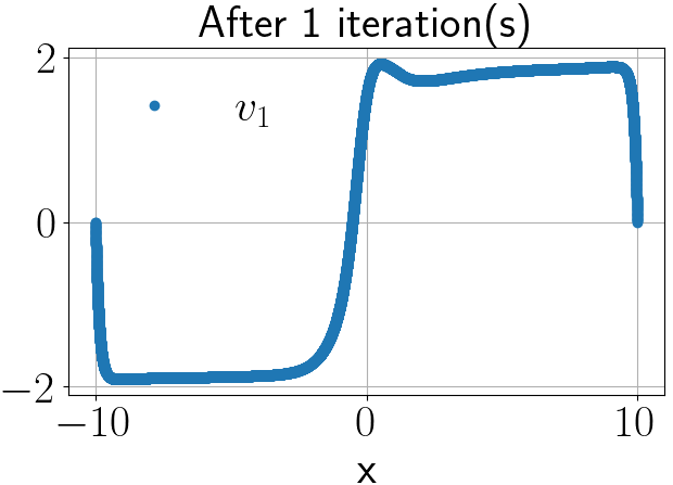
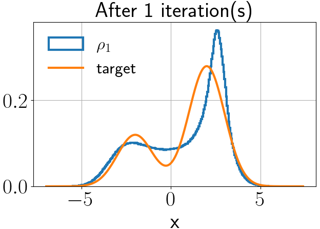
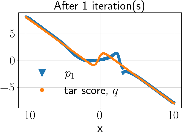
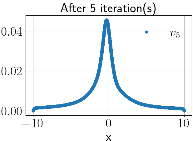
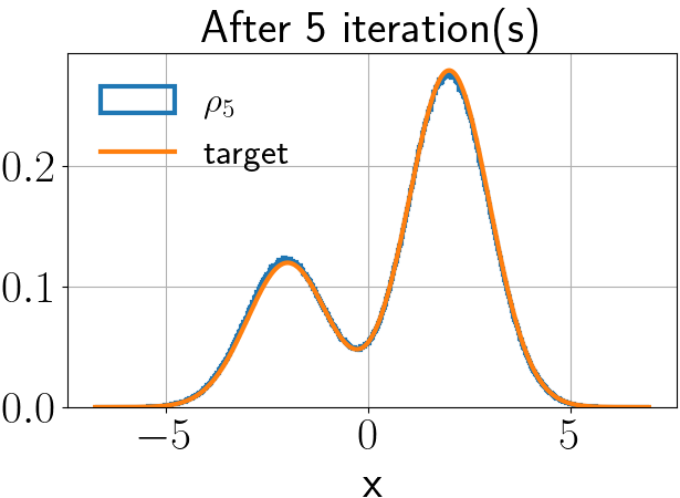
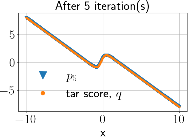
Figure 2: Left: the solution $v_{n}$ after 1 (top) and 5 (bottom) iterations computed using second order finite difference with O(500) grid points. Center: the transformed empirical density. Right: $p_{1}$ (top) and $p_{5}$ (bottom).

5 Numerical results

Here we present proof-of-concept numerical results that demonstrate the convergence of our SCONE transport (Algorithm 1). On 1D domains, we find that the SCONE transport map converges to the monotone map or the increasing rearrangement, which is optimal with respect to any convex cost (see Chapter 2 of Santambrogio [2015]). We also demonstrate that SCONE transport maps can effectively tackle multimodality in the target. See Appendix C for details on the numerical methods and additional experiments.

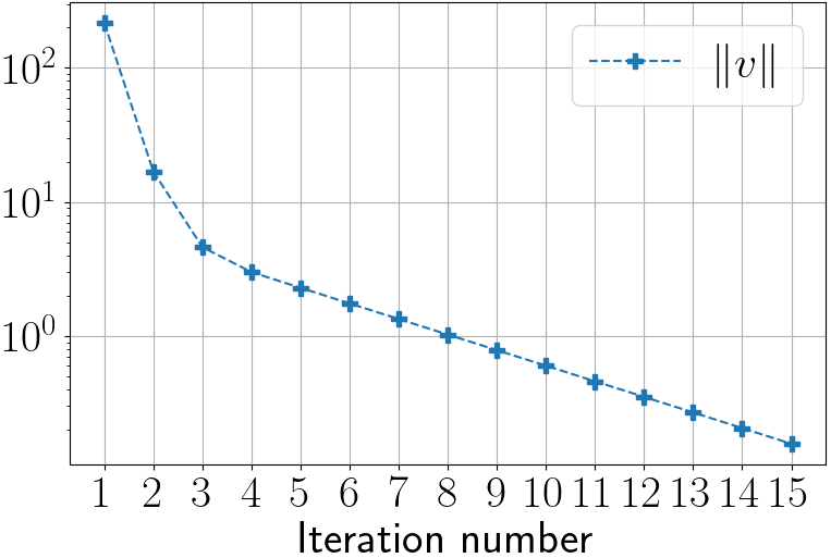
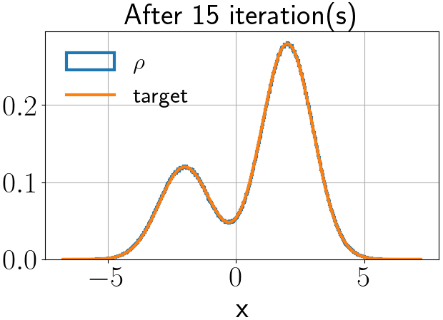
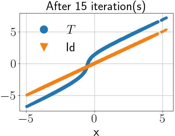
Figure 3: Convergence of SCONE. Left: the convergence of $\|v_{n}\|$. Center: transformed empirical density after 15 iterations. Right: $T_{n}$ after 15 iterations.

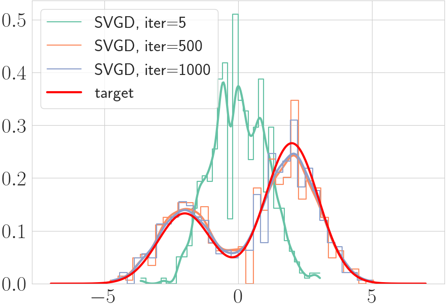
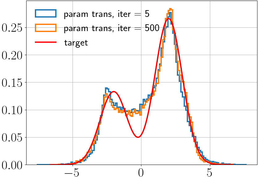
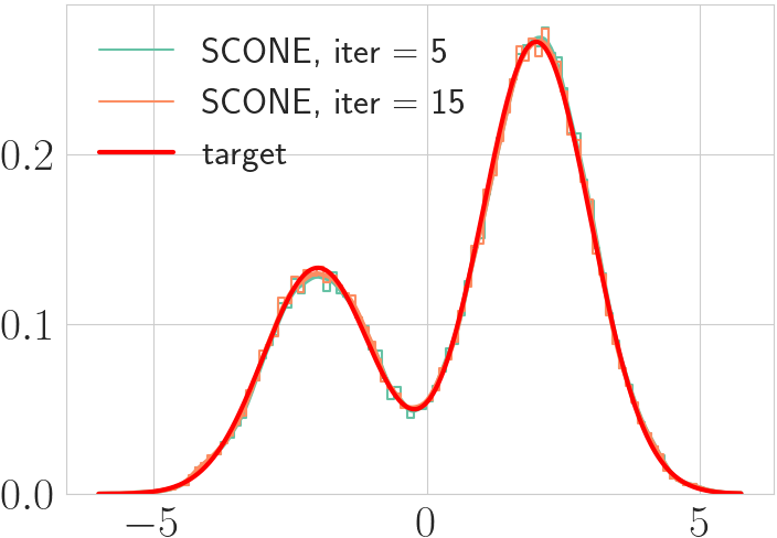
Figure 4: Left: SVGD with RBF kernels (median heuristic for bandwidth) and 512 particles. Center: parameterized monotone transport map [Parno et al., 2022], with polynomial degree 10, 512²/11 samples, optimized using gradient descent + line search. Right: SCONE transport with ODE updates solved with 512 grid points.

In Figure 2, we show the results of applying the SCONE algorithm to a bimodal target density of the form $w_{1}\mathcal{N}(m_{1},\sigma_{1}^{2})+w_{2}\mathcal{N}(m_{2},\sigma_{2}^{2})$ (shown in orange in the center column). The target score is shown in orange on the right column. We see from the second row of Figure 2 that the transformed scores and densities match those of the target closely after just 5 iterations. We observe numerically that solving the SCONE step (10) (which reduces to an ODE in 1D) on a coarser grid (of size ${\cal O}(100)$) does not affect fast convergence when we add a small $\ell^{2}$ regularization. In comparison, SVGD takes ${\cal O}(500)$ iterations [Liu and Wang, 2016] with 100 particles for the same problem, and a vanilla GAN implementation [Goodfellow et al., 2020] can lead to unstable training and mode collapse [Thanh-Tung and Tran, 2020, Li et al., 2018]. In Figure 3, we show the convergence of the SCONE algorithm to the target. We see that the identified transport map converges to the optimal map (shown in blue in the right column).

Comparison with other algorithms In Figure 4, we compare SCONE against SVGD [Liu and Wang, 2016] and parameterized transport maps [Parno et al., 2022] as these are the most widely used classes of algorithms for Bayesian inference. With $N$ samples, an SVGD iteration has ${\cal O}(N^{2})$ cost. With $G$ grid points, SCONE iterations have ${\cal O}(G^{2})$ cost, since the linear system to be solved at a SCONE iteration is banded. With $P$ parameters and $S$ samples to evaluate the variational (KL) objective, the optimization step for a parameterized transport map is ${\cal O}(PS).$ We choose $PS=N^{2}=G^{2}=512^{2}$ so that the computational budget per iteration remains the same across the different methods. We see in Figure 4 (right) that densities obtained from SCONE most closely match the target (red) after just 5 iterations, while SVGD (left) takes ${\cal O}(500)$ iterations to converge to a comparatively worse solution. Parameterized transport (center) converges quickly, with the help of a backtracking line search optimization, but makes a significant approximation error which persists even for higher polynomial degree (we tested up to 20). Figure 4 thus demonstrates that SCONE vastly outperforms SVGD and parameterized transport algorithms for the same computational cost.

6 Discussion

We introduce a new notion of infinite-dimensional score-matching that yields a Newton-type method for sampling, and we prove sufficient conditions for its convergence. Our method applies in settings where scores of the source and target measures are easily computed. We comment on theoretical and algorithmic features of this work that will spur further research.

Learning elliptic PDEs: Many structure-exploiting, fast, and sample-efficient methods are emerging for learning the solution operators of linear elliptic PDEs; see, e.g., Lu et al. [2021a], Boullé and Townsend [2023], Schäfer and Owhadi [2021]. These methods use randomized numerical linear algebra [Boullé and Townsend, 2023], CNN-based encoder-decoder networks [Zhang and Garikipati, 2023], interpolation between deep neural network and Monte Carlo approximations [Nüsken and Richter, 2023], etc. These results suggest that it is possible to develop optimal methods, in terms of computational and sample complexity, for learning our SCONE update operator $\mathcal{L}(q)^{-1}$ by exploiting low-rank structure in its solutions. With the same goal, we will also explore particle methods (e.g., from fluid dynamics [Monaghan, 2012, Cottet et al., 2000]), which can also use fast numerical linear algebra and have theoretical guarantees.

Newton convergence: Under typical conditions, the classical result of Kantorovich (see Galántai [2000] for a survey) establishes quadratic convergence starting in a ball of sufficiently small radius (as in our Theorem 3). In future work, we will investigate damping and modified SCONE iterations to prevent divergence [Smale, 1985]. We will also develop inexact and quasi-Newton variants of SCONE, as a way of further reducing computational cost [Traub and Woźniakowski, 1980] and allowing for errors in $q.$ We will derive theoretical convergence guarantees for these modified SCONEs.

Appendix A Other iterations based on the contraction mapping principle

For a fixed $p$, the score operator, $\mathcal{G}(p,\cdot)$, is a map from the space of transformations to scores. We first define a self-map corresponding to the score-residual operator. Then, we define a fixed point iteration for the self-map that converges in a setting where it is a contraction.

For convenience, we denote by $\mathcal{G}_{p}$ the operator $\mathcal{G}(p,\cdot)$ that returns the transported score, given a transport map. Let $\mathbb{T}$ be a Banach space of functions on $\mathbb{R}^{d}$ and $\mathbb{S}$ a Banach space of scores. Using the definition of the score operator,

$$\mathcal{G}_{p}(T)\circ T=p(\nabla T)^{-1}-{\rm tr}((\nabla T)^{-1}\>\nabla^{2}T)\>(\nabla T)^{-1}=q\circ T,$$ (24)

when $T$ is a solution of the score-matching problem. We assume that the target score $q$ is a homeomorphism onto its image. This is indeed a strong condition that multi-modal distributions, for example, do not satisfy. Define a self-map $\mathcal{H}:\mathbb{T}\to\mathbb{T}$

$$\mathcal{H}(T)=q^{-1}\circ\mathcal{G}_{p}(T)\circ T.$$ (25)

Clearly, if $T$ is a solution of the score-matching problem, it is a fixed point of $\mathcal{H}$. Near a fixed point, we can define the following fixed-point iteration of $\mathcal{H}$.

$$T_{n+1}=\mathcal{H}(T_{n})=q^{-1}\circ\mathcal{G}_{p}(T_{n})\circ T_{n},$$ (26)

with an arbitrary map $T_{0}$. When $\mathcal{H}$ is a contraction near its fixed point, say, $T^{*}$, then $T_{n}$ defined in (26) converges to $T^{*}$, by the contraction mapping principle. Consider one sufficient condition: when the functional derivative $D(\mathcal{G}_{p}(T)\circ T)(T^{*})$ and the gradient $\nabla q^{-1}$ are small in the operator norms and $C^{0}$ norm respectively. Then, one obtains that $\mathcal{H}$ is contraction, and hence the fixed-point iteration defined above converges to a fixed point or a transport map.

However, this is only a sufficient condition for convergence. When $\mathcal{H}$ is not contractive, the fixed point iterations may not converge, or may exhibit slower than exponential convergence. When $\mathbb{T}$ is large enough to contain multiple fixed points of $\mathcal{H}$, the iterations may oscillate between basins of attraction of multiple fixed points. Note that the sufficient conditions for $\mathcal{H}$ to be a contraction impose restrictions on the behavior of the score operator near the fixed point and on the second-order derivatives of the target, which may preclude multi-modality in the target. The SCONE method, on the other hand, does not explicitly impose such a restriction at the fixed point and is hence more general.

Appendix B SCONE example

As the first example, suppose the target is a univariate Gaussian with mean $m$ and variance $s^{2}$, while the source distribution is a standard normal in 1D. In this case, $q(x)=-(x-m)/s^{2}$ and $p(x)=-x$. The SCONE update $v_{n}$ satisfies the following ODE:

$$p_{n}-q=v_{n}^{\prime\prime}+qv_{n}^{\prime}+q^{\prime}v_{n}.$$ (27)

At $n=0$, $p_{n}=p$. The above ODE is defined on an unbounded domain, without specific decay rates for the solution at the boundaries, $\pm\infty$. This allows for unbounded solutions. Notice that the solution is always affine since, at $n=0$, the left-hand side is affine. Subsequently, the update equation is satisfied by affine functions $v_{n}$ at every $n$ and hence $T_{n}$, which is a composition of affine functions, is affine. By comparing coefficients to solve for the update equations, we can obtain recurrence relationships for the slopes and intercepts of $v_{n}$, $T_{n+1}\coloneqq({\rm Id}+v_{n})\circ T_{n}$, and $p_{n}=(p/T_{n}^{\prime})\circ T_{n}^{-1}$. We can inductively show that all three are affine functions for all $n$. In particular, if $p_{n}(x)=a_{n}x+b_{n}$ and $v_{n}(x)=(A_{n}-1)x+B_{n}$, we obtain,

$$A_{n} =-a_{n}s^{2}/2+1/2$$

$$B_{n} =-b_{n}s^{2}+m/2-a_{n}ms^{2}/2,$$

by comparing coefficients in the update (27). Then, the update for the score gives,

$$a_{n+1}=a_{n}/A_{n}^{2},b_{n+1}=-a_{n}B_{n}/A_{n}^{2}+B_{n}/A_{n}^{2}.$$

Considering the set of sequences $\{a_{n},b_{n},A_{n},B_{n}\}_{n}$, it is clear from the relationships above that when $A_{n}\to 1$ and $B_{n}\to 0$, $a_{n}\to(-1/s^{2})$ and $b_{n}\to m/s^{2}$. Thus, when the iterations for $T_{n}$ converge, or equivalently, when $v_{n}\to 0$, $p_{n}\to q$. Moreover, in this case, the limit $T$ is the function $T(x)=sx+m$, which coincides with the increasing rearrangement on $\mathbb{R}$ (and hence the optimal map). The intermediate distributions corresponding to the scores $p_{n}$ are all Gaussian.

Notice that since this convergence can be established for all $s$ and $m$, it suggests that SCONE transport converges even when in Hölder norm, $\|p-q\|$ is not small. That is, even though the derivation of the is premised on the local expansion of the score operator around $(q,{\rm Id})$, the smallness of $p-q$ and $T-{\rm Id}$ is not a necessary condition for the convergence of the method.

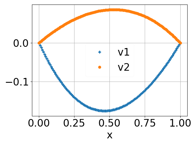
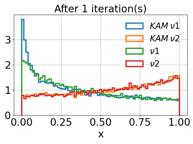
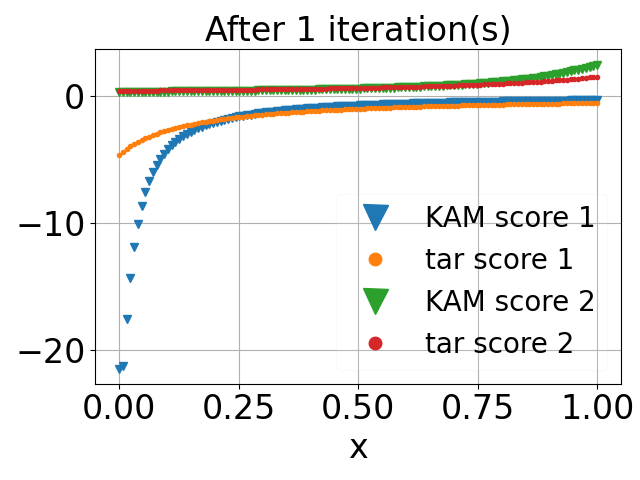
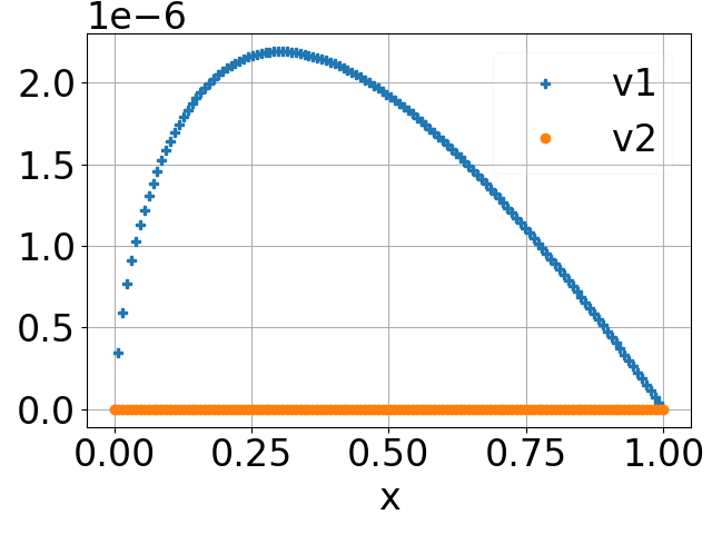
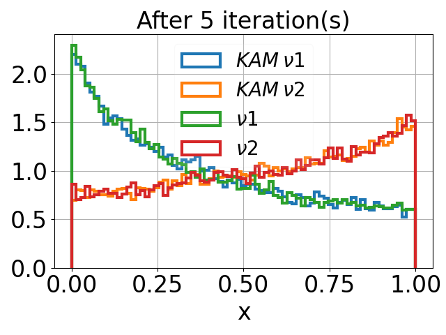
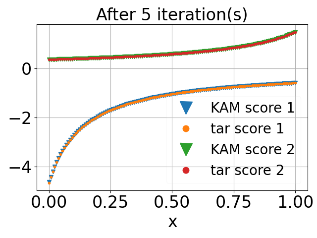
Figure 5: Numerical validation of SCONE transport on 1D densities: the first row depicts results after 1 iteration of our Newton method and the second row after 5 iterations. The scalar field $v,$ the histogram approximations of the target density and the target score are plotted for the two different targets described in section C. The results of the computed transformed densities and scores from the SCONE iteration are compared against the target densities and scores in columns 2 and 3.

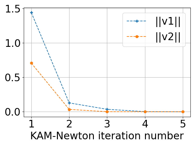
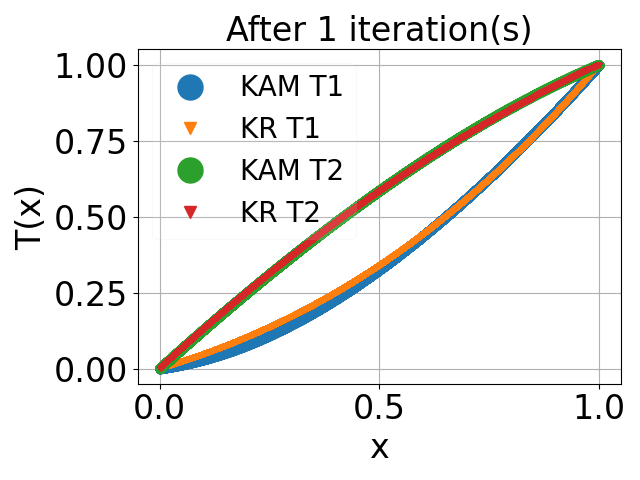
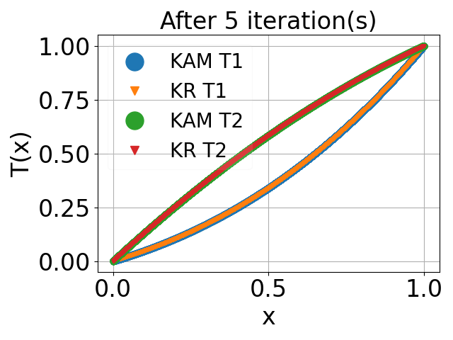
Figure 6: On the left column, we show the convergence of our algorithm ($\|v_{n}\|\to 0$) for the two different target densities given in section C. The center and right hand side figures compare the optimal map computed analytically against the SCONE transport map computed numerically after one and five iterations respectively.

Appendix C Additional experiments

Considering 1D targets, we first give proof-of-concept numerical results to validate our SCONE construction. We consider two smooth densities supported on $[0,1]$ as our targets: $\rho_{\nu 1}=((x+1)^{3}-1)/7$ and $\rho_{\nu 2}=4/3-(2-x)^{2}/3.$ These densities are shown as histograms in the second column of Figure 5. In 1D, the PDE that needs to be solved at every SCONE iteration is an ODE, which we solve using a finite difference method with 128 grid points and zero Dirichlet boundary conditions on $[0,1].$ Our source density is the uniform (Lebesgue) density on $[0,1]$ whose score is the zero function. As shown in Figure 5 (third column), the transformed score matches the target score within a few SCONE iterations. The solution $v$ also quickly approaches the zero function as confirmed in the first column of Figure 5 and Figure 6(left), thus establishing numerically the convergence of our construction (see Theorem 3 in the main text). On one-dimensional domains, the optimal transport map (for a variety of costs) is simply the increasing rearrangement (see [Santambrogio, 2015], Chapter 2), which can be computed analytically in our setting, and is shown in the second and third columns of Figure 6. As shown, the SCONE construction converges to this transport map.

C.1 1D unbounded target: bimodal Gaussian with equally weighted modes

Next, we consider a one-dimensional bimodal Gaussian target (shown in Figure 7), $0.5\mathcal{N}(-2,1)+0.5\mathcal{N}(2,1)$. We again solve the ODE with finite difference on $[-10,10]$. The source is taken to be the standard Gaussian (unimodal distribution). In Figure 7, the first row presents results obtained after 1 iteration of our SCONE algorithm; the second row, after 3 iterations. We see that, after just 1 iteration, the two modes are detected, although the density and scores are not well-approximated. After 3 iterations, the empirical density (shown in blue) of the samples transported by the SCONE transport map match the target density (orange line plot) closely. As shown in Figure 7 (second row), as the SCONE update solution $v$ declines, the density and the scores approach their target values. In Figure 8 (left), we show the convergence of the solution $v$. From the figure, the convergence appears to be exponentially fast, with the rate decreasing after the first 4 iterations. The final transport map (right) is taken after 5 iterations, which accurately models the target density (center). A grid size of 4096 is used for solving the SCONE iteration, but grid size reductions ${\cal O}(1000)$ produces similar convergence results. We find that more iterations are needed when the modes are well-separated, e.g., sampling from an equally weighted bimodal distribution with modes centered at -4 and 2 required around 20 iterations.

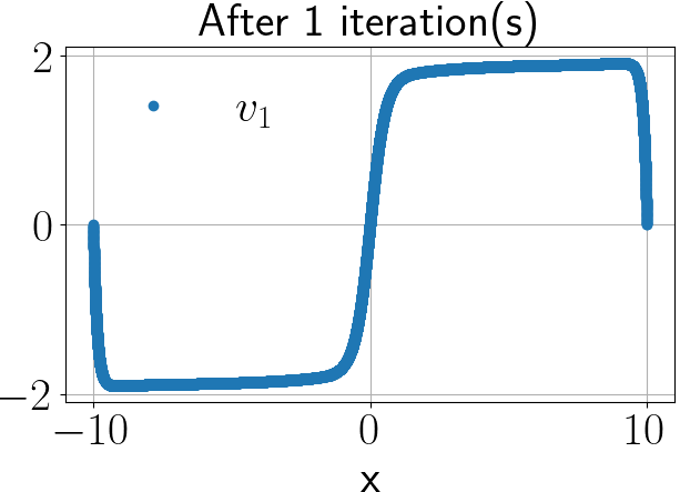
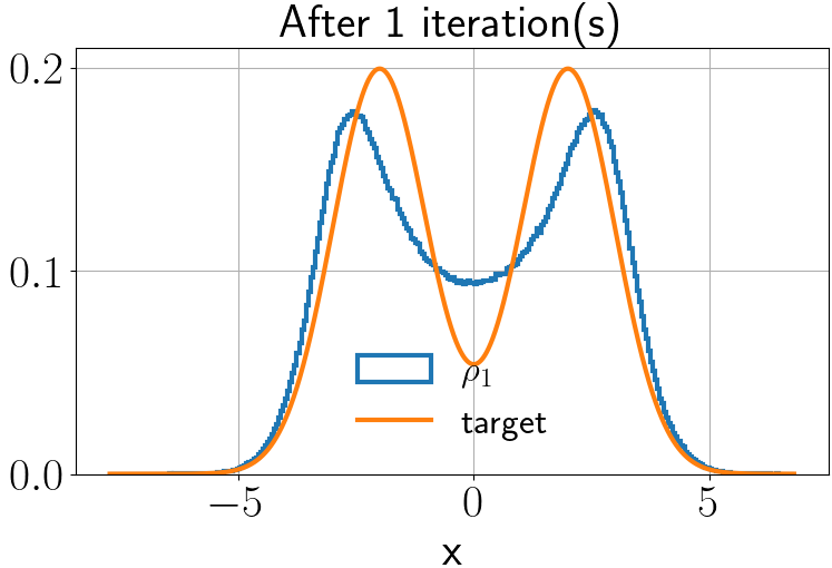
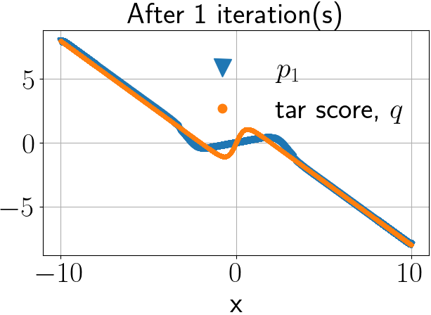
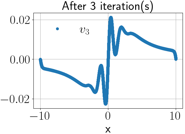
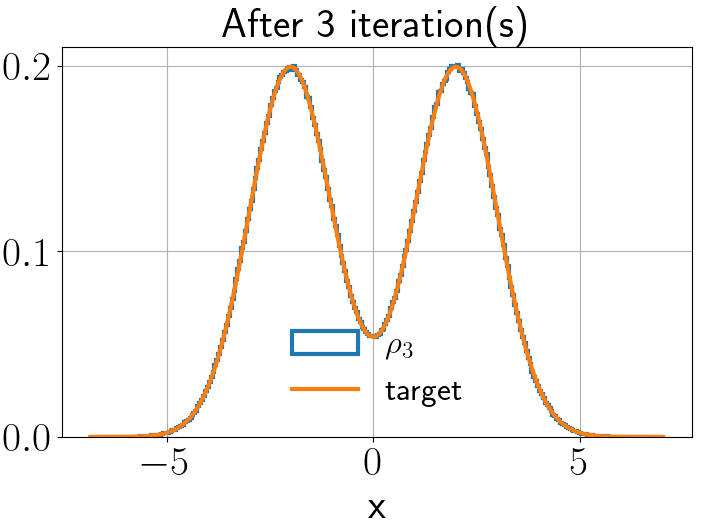
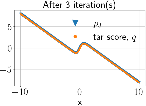
Figure 7: SCONE algorithm results: the target distribution, shown in orange in the center column, is an equally weighted bimodal Gaussian. The application of the SCONE algorithm, as described in section C.1, is shown in the first row after 1 iteration and in the second row after 3 iterations. The scalar field $v,$ the histogram approximations of the target density and the target score are plotted in the first, second and third columns, respectively. The results of the computed transformed densities and scores from the SCONE iteration are compared against the target densities and scores in columns 2 and 3.

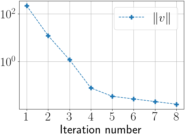
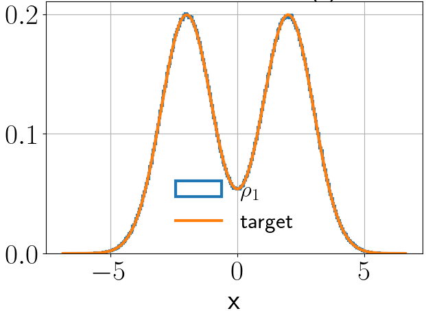
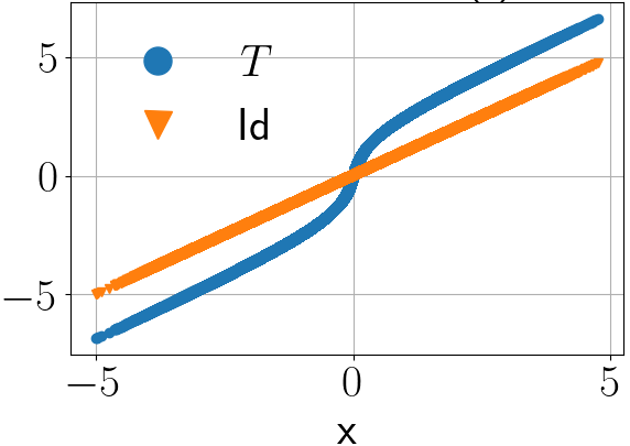
Figure 8: Convergence of SCONE iteration: the target distribution, shown in orange in the center column, is an equally weighted bimodal Gaussian. The application of the SCONE algorithm, as described in section C.1, results in the convergence of $\|v_{n}\|$, shown in the first column. The final SCONE transport map after 5 iterations is on the right (blue).

C.2 1D unbounded target: bimodal Gaussian with unequally weighted modes

Previously in section C.1, when the target consisted of equally weighted modes, we used a finite difference method to solve the ODE, and then function interpolation to evaluate $v$ at the samples. Using these interpolated values, the score function, $p$ was updated, and the iterations continued by solving the ODE again. This vanilla scheme leads to numerical blow-up when the target has unequal weights. The reason is that errors in the solution of $v$ leads to the divergence of our Newton-like method. We observe that adding a small regularization term in the finite-difference ODE solution ($\ell^{2}$ regularization parameter set to 0.01), along with refining the grid near the points where $q^{\prime}$ is large, induces convergence. The results are in the main text (section 5).

We provide the source code implementing the SCONE algorithm on all the examples above in [Chandramoorthy, 2023]. This contains ‘oneD.py’ that implements the SCONE algorithm on all the examples above. The source file ‘oneD_nonUni.py’ implements adaptive grid refinement in the finite-difference solver. The unit tests that generate all the figures in this section are in ‘tests/test_1D.py’. The code is written in Python and uses numpy and scipy.

References

- Albergo et al. [2023] Michael S Albergo, Nicholas M Boffi, and Eric Vanden-Eijnden. Stochastic interpolants: A unifying framework for flows and diffusions. arXiv preprint arXiv:2303.08797, 2023.
- Berti and Bolle [2015] Massimiliano Berti and Philippe Bolle. A Nash-Moser approach to KAM theory. Hamiltonian partial differential equations and applications, pages 255–284, 2015.
- Boullé and Townsend [2023] Nicolas Boullé and Alex Townsend. Learning elliptic partial differential equations with randomized linear algebra. Foundations of Computational Mathematics, 23(2):709–739, 2023.
- Chandramoorthy [2023] Nisha Chandramoorthy. ni-sha-c/score-based-transport: v1, December 2023. URL https://doi.org/10.5281/zenodo.10307262.
- Chandramoorthy and Wang [2022] Nisha Chandramoorthy and Qiqi Wang. Efficient computation of linear response of chaotic attractors with one-dimensional unstable manifolds. SIAM Journal on Applied Dynamical Systems, 21(2):735–781, 2022. doi:10.1137/21M1405599. URL https://doi.org/10.1137/21M1405599.
- Chen and Ghattas [2020] Peng Chen and Omar Ghattas. Projected Stein variational gradient descent. Advances in Neural Information Processing Systems, 33:1947–1958, 2020.
- Chen et al. [2018] Ricky TQ Chen, Yulia Rubanova, Jesse Bettencourt, and David K Duvenaud. Neural ordinary differential equations. Advances in neural information processing systems, 31, 2018.
- Chewi et al. [2020] Sinho Chewi, Thibaut Le Gouic, Chen Lu, Tyler Maunu, and Philippe Rigollet. SVGD as a kernelized Wasserstein gradient flow of the chi-squared divergence. Advances in Neural Information Processing Systems, 33:2098–2109, 2020.
- Ciarlet [2002] Philippe G Ciarlet. The finite element method for elliptic problems. SIAM, 2002.
- Cottet et al. [2000] Georges-Henri Cottet, Petros D Koumoutsakos, et al. Vortex methods: theory and practice, volume 8. Cambridge university press Cambridge, 2000.
- Dahmen et al. [2016] W. Dahmen, R. DeVore, L. Grasedyck, and E. Süli. Tensor-sparsity of solutions to high-dimensional elliptic partial differential equations. Found Comput Math, 16:813–874, 2016. doi:10.1007/s10208-015-9265-9.
- Detommaso et al. [2018] Gianluca Detommaso, Tiangang Cui, Youssef Marzouk, Alessio Spantini, and Robert Scheichl. A Stein variational Newton method. Advances in Neural Information Processing Systems, 31, 2018.
- Duncan et al. [2019] Andrew Duncan, Nikolas Nüsken, and Lukasz Szpruch. On the geometry of Stein variational gradient descent. arXiv preprint arXiv:1912.00894, 2019.
- Dyatlov [2022] Semyon Dyatlov. Lecture notes for 18.155: distributions, elliptic regularity, and applications to pdes. https://math.mit.edu/~dyatlov/18.155/155-notes.pdf, 2022. [Online; accessed Jan 20th, 2023].
- Evans [2022] Lawrence C Evans. Partial differential equations, volume 19. American Mathematical Society, 2022.
- Galántai [2000] A. Galántai. The theory of newton’s method. Journal of Computational and Applied Mathematics, 124(1):25–44, 2000. ISSN 0377-0427. doi:https://doi.org/10.1016/S0377-0427(00)00435-0. URL https://www.sciencedirect.com/science/article/pii/S0377042700004350. Numerical Analysis 2000. Vol. IV: Optimization and Nonlinear Equations.
- Gerlach [1994] Jürgen Gerlach. Accelerated convergence in newton’s method. Siam Review, 36(2):272–276, 1994.
- Giaquinta and Martinazzi [2013] Mariano Giaquinta and Luca Martinazzi. An introduction to the regularity theory for elliptic systems, harmonic maps and minimal graphs. Springer Science & Business Media, 2013.
- Gilbarg and Trudinger [1977] David Gilbarg and Neil S Trudinger. Elliptic partial differential equations of second order, volume 224. Springer, 1977.
- Goodfellow et al. [2020] Ian Goodfellow, Jean Pouget-Abadie, Mehdi Mirza, Bing Xu, David Warde-Farley, Sherjil Ozair, Aaron Courville, and Yoshua Bengio. Generative adversarial networks. Communications of the ACM, 63(11):139–144, 2020.
- Han and Liu [2017] Jun Han and Qiang Liu. Stein variational adaptive importance sampling. arXiv preprint arXiv:1704.05201, 2017.
- Hörmander [1963] Lars Hörmander. Elliptic boundary problems, pages 242–274. Springer Berlin Heidelberg, Berlin, Heidelberg, 1963. ISBN 978-3-642-46175-0. doi:10.1007/978-3-642-46175-0_10. URL https://doi.org/10.1007/978-3-642-46175-0_10.
- Huang et al. [2020] Chin-Wei Huang, Ricky TQ Chen, Christos Tsirigotis, and Aaron Courville. Convex potential flows: Universal probability distributions with optimal transport and convex optimization. arXiv preprint arXiv:2012.05942, 2020.
- Hyvärinen and Dayan [2005] Aapo Hyvärinen and Peter Dayan. Estimation of non-normalized statistical models by score matching. Journal of Machine Learning Research, 6(4), 2005.
- Iglesias and Yang [2021] Marco Iglesias and Yuchen Yang. Adaptive regularisation for ensemble kalman inversion. Inverse Problems, 37(2):025008, 2021.
- Jordan et al. [1998] Richard Jordan, David Kinderlehrer, and Felix Otto. The variational formulation of the Fokker–Planck equation. SIAM Journal on Mathematical Analysis, 29(1):1–17, 1998. doi:10.1137/S0036141096303359. URL https://doi.org/10.1137/S0036141096303359.
- Kingma et al. [2019] Diederik P Kingma, Max Welling, et al. An introduction to variational autoencoders. Foundations and Trends® in Machine Learning, 12(4):307–392, 2019.
- Li et al. [2018] Jerry Li, Aleksander Madry, John Peebles, and Ludwig Schmidt. On the limitations of first-order approximation in gan dynamics. In International Conference on Machine Learning, pages 3005–3013. PMLR, 2018.
- Li et al. [2020a] Lei Li, Yingzhou Li, Jian-Guo Liu, Zibu Liu, and Jianfeng Lu. A stochastic version of Stein variational gradient descent for efficient sampling. Communications in Applied Mathematics and Computational Science, 15(1):37–63, 2020a.
- Li et al. [2020b] Zongyi Li, Nikola Kovachki, Kamyar Azizzadenesheli, Burigede Liu, Kaushik Bhattacharya, Andrew Stuart, and Anima Anandkumar. Fourier neural operator for parametric partial differential equations. arXiv preprint arXiv:2010.08895, 2020b.
- Liu and Wang [2016] Qiang Liu and Dilin Wang. Stein variational gradient descent: A general purpose Bayesian inference algorithm. Advances in neural information processing systems, 29, 2016.
- Lu et al. [2021a] Yiping Lu, Haoxuan Chen, Jianfeng Lu, Lexing Ying, and Jose Blanchet. Machine learning for elliptic pdes: Fast rate generalization bound, neural scaling law and minimax optimality. arXiv preprint arXiv:2110.06897, 2021a.
- Lu et al. [2021b] Yulong Lu, Jianfeng Lu, and Min Wang. A priori generalization analysis of the deep ritz method for solving high dimensional elliptic partial differential equations. In Conference on learning theory, pages 3196–3241. PMLR, 2021b.
- Masrani et al. [2021] Vaden Masrani, Rob Brekelmans, Thang Bui, Frank Nielsen, Aram Galstyan, Greg Ver Steeg, and Frank Wood. q-paths: Generalizing the geometric annealing path using power means. In Uncertainty in Artificial Intelligence, pages 1938–1947. PMLR, 2021.
- Monaghan [2012] Joseph J Monaghan. Smoothed particle hydrodynamics and its diverse applications. Annual Review of Fluid Mechanics, 44:323–346, 2012.
- Morrey [1953] Charles B. Morrey. Second order elliptic systems of differential equations. Proceedings of the National Academy of Sciences, 39(3):201–206, 1953. doi:10.1073/pnas.39.3.201. URL https://www.pnas.org/doi/abs/10.1073/pnas.39.3.201.
- Moser [1961] Jurgen Moser. A new technique for the construction of solutions of nonlinear differential equations. Proceedings of the National Academy of Sciences, 47(11):1824–1831, 1961.
- Ni [2020] Angxiu Ni. Fast linear response algorithm for differentiating chaos, 2020. URL https://arxiv.org/abs/2009.00595.
- Nüsken and Richter [2023] Nikolas Nüsken and Lorenz Richter. Interpolating between bsdes and pinns: deep learning for elliptic and parabolic boundary value problems, 2023.
- Owhadi and Scovel [2019] Houman Owhadi and Clint Scovel. Operator-Adapted Wavelets, Fast Solvers, and Numerical Homogenization: From a Game Theoretic Approach to Numerical Approximation and Algorithm Design, volume 35. Cambridge University Press, 2019.
- Papamakarios et al. [2021] George Papamakarios, Eric Nalisnick, Danilo Jimenez Rezende, Shakir Mohamed, and Balaji Lakshminarayanan. Normalizing flows for probabilistic modeling and inference. The Journal of Machine Learning Research, 22(1):2617–2680, 2021.
- Parno et al. [2022] Matthew Parno, Paul-Baptiste Rubio, Daniel Sharp, Michael Brennan, Ricardo Baptista, Henning Bonart, and Youssef Marzouk. Mpart: Monotone parameterization toolkit. Journal of Open Source Software, 7(80):4843, 2022.
- Raissi et al. [2019] Maziar Raissi, Paris Perdikaris, and George E Karniadakis. Physics-informed neural networks: A deep learning framework for solving forward and inverse problems involving nonlinear partial differential equations. Journal of Computational physics, 378:686–707, 2019.
- Reich [2011] Sebastian Reich. A dynamical systems framework for intermittent data assimilation. BIT Numerical Mathematics, 51:235–249, 2011.
- Santambrogio [2015] Filippo Santambrogio. Optimal transport for applied mathematicians. Birkäuser, NY, 55(58-63):94, 2015.
- Schaback and Wendland [2006] Robert Schaback and Holger Wendland. Kernel techniques: from machine learning to meshless methods. Acta numerica, 15:543–639, 2006.
- Schäfer and Owhadi [2021] Florian Schäfer and Houman Owhadi. Sparse recovery of elliptic solvers from matrix-vector products. arXiv preprint arXiv:2110.05351, 2021.
- Smale [1985] Steve Smale. On the efficiency of algorithms of analysis. Bulletin of the American Mathematical Society, 13(2):87–121, 1985.
- Song et al. [2020a] Jiaming Song, Chenlin Meng, and Stefano Ermon. Denoising diffusion implicit models. ArXiv, abs/2010.02502, 2020a. URL https://api.semanticscholar.org/CorpusID:222140788.
- Song and Ermon [2019] Yang Song and Stefano Ermon. Generative modeling by estimating gradients of the data distribution. Advances in Neural Information Processing Systems, 32, 2019.
- Song et al. [2020b] Yang Song, Jascha Sohl-Dickstein, Diederik P Kingma, Abhishek Kumar, Stefano Ermon, and Ben Poole. Score-based generative modeling through stochastic differential equations. arXiv preprint arXiv:2011.13456, 2020b.
- Thanh-Tung and Tran [2020] Hoang Thanh-Tung and Truyen Tran. Catastrophic forgetting and mode collapse in gans. In 2020 international joint conference on neural networks (ijcnn), pages 1–10. IEEE, 2020.
- Traub and Woźniakowski [1980] JF Traub and H Woźniakowski. Convergence and complexity of interpolatory—newton iteration in a banach space. Computers & Mathematics with Applications, 6(4):385–400, 1980.
- Villa et al. [2021] Umberto Villa, Noemi Petra, and Omar Ghattas. HIPPYlib: an extensible software framework for large-scale inverse problems governed by PDEs. ACM Transactions on Mathematical Software (TOMS), 47(2):1–34, 2021.
- Wang and Ye [2013] Junping Wang and Xiu Ye. A weak galerkin finite element method for second-order elliptic problems. Journal of Computational and Applied Mathematics, 241:103–115, 2013.
- Wendland [2004] Holger Wendland. Scattered data approximation, volume 17. Cambridge university press, 2004.
- Wibisono [2018] Andre Wibisono. Sampling as optimization in the space of measures: The Langevin dynamics as a composite optimization problem. In Conference on Learning Theory, pages 2093–3027. PMLR, 2018.
- Wibisono and Yang [2022] Andre Wibisono and Kaylee Yingxi Yang. Convergence in kl divergence of the inexact Langevin algorithm with application to score-based generative models, 2022. URL https://arxiv.org/abs/2211.01512.
- Yu et al. [2018] Bing Yu et al. The deep ritz method: a deep learning-based numerical algorithm for solving variational problems. Communications in Mathematics and Statistics, 6(1):1–12, 2018.
- Zhang and Garikipati [2023] Xiaoxuan Zhang and Krishna Garikipati. Label-free learning of elliptic partial differential equation solvers with generalizability across boundary value problems. Computer Methods in Applied Mechanics and Engineering, page 116214, 2023. ISSN 0045-7825. doi:https://doi.org/10.1016/j.cma.2023.116214. URL https://www.sciencedirect.com/science/article/pii/S0045782523003389.
- Zhang et al. [2000] Xiong Zhang, Kang Zhu Song, Ming Wan Lu, and X Liu. Meshless methods based on collocation with radial basis functions. Computational mechanics, 26:333–343, 2000.