Diversity, Agreement, and Polarization in Elections

Abstract

We consider the notions of agreement, diversity, and polarization in ordinal elections (that is, in elections where voters rank the candidates). While (computational) social choice offers good measures of agreement between the voters, such measures for the other two notions are lacking. We attempt to rectify this issue by designing appropriate measures, providing means of their (approximate) computation, and arguing that they, indeed, capture diversity and polarization well. In particular, we present “maps of preference orders” that highlight relations between the votes in a given election and which help in making arguments about their nature.

1   Introduction

The notions of agreement, diversity, and polarization of a society with respect to some issue are intuitively quite clear. In case of agreement, most members of the society have very similar views regarding the issue, in case of diversity there is a whole spectrum of opinions, and in case of polarization there are two opposing camps with conflicting views and with few people taking middle-ground positions (more generally, if there are several camps, with clearly separated views, then we speak of fragmentation; see, for example, the collection of Dynes and Tierney (1994)). We study these three notions for the case of ordinal elections—that is, for elections where each voter has a preference order (his or her vote) ranking the candidates from the most to the least appealing one—and analyze ways of quantifying them.

Interestingly, even though agreement, diversity, and polarization seem rather fundamental concepts for understanding the state of a given society (see, for example, the papers in a special issue edited by Levin et al. (2021)), so far (computational) social choice mostly focused on the agreement-disagreement spectrum. Let us consider the following notion:

• Given an election, the voters’ agreement index for candidates $a$ and $b$ is the absolute value of the difference between the fraction of the voters who prefer $a$ to $b$ and the fraction of those with the opposite view. Hence, if all voters rank $a$ over $b$ (or, all voters rank $b$ over $a$) then the agreement index for these candidates is equal to $1$. On the other hand, if half of the voters report $a\succ b$ and half of them report $b\succ a$, then the index is equal to $0$. The agreement index of the whole election is the average over the agreement indices of all the candidate pairs.

For an election $E$, we denote its agreement index as $A(E)$. Alcalde-Unzu and Vorsatz (2013) viewed this index as measuring voter cohesiveness—which is simply a different term for voter agreement—and provided its axiomatic characterization. Hashemi and Endriss (2014) focused on measuring diversity and provided axiomatic and experimental analyses of a number of election indices, including $1-A(E)$. $1-A(E)$ was also characterized axiomatically by Can et al. (2015), who saw it as measuring polarization; their point of view was that for each pair of candidates one can measure polarization independently. (In Section 2 we briefly discuss other election indices from the literature; generally, they are strongly interrelated with the agreement one).

Our view is that $1-A(E)$ is neither a measure of diversity nor of polarization, but of disagreement. Indeed, it has the same, highest possible, value on both the antagonism election (AN), where half of the voters report one preference order and the other half reports the opposite one, and on the uniformity election (UN), where each possible preference order occurs the same number of times. Indeed, both these elections arguably represent extreme cases of disagreement. Yet, the nature of this disagreement is very different. In the former, we see strong polarization, with the voters taking one of the two opposing positions, and in the latter we see perfect diversity of opinion. The fundamental difference between these notions becomes clear in the text of Levin et al. (2021) which highlights “the loss of diversity that extreme polarization creates” as a central theme of the related special issue. Our main goal is to design election indices that distinguish these notions.

Our new indices are based on what we call the $k$-Kemeny problem. In the classic Kemeny Ranking problem (equivalent to $1$-Kemeny), given an election we ask for a ranking whose sum of swap distances to the votes is the smallest (a swap distance between two rankings is the number of swaps of adjacent candidates needed to transform one ranking into the other). The $k$-Kemeny problem is defined analogously, but we ask for $k$ rankings that minimize the sum of each vote’s distance to the closest one (readers familiar with multiwinner elections (Faliszewski et al., 2017) may think of it as the Chamberlin–Courant rule (Chamberlin and Courant, 1983) for committees of rankings rather than candidates). We refer to this value as the $k$-Kemeny distance. Unfortunately, the $k$-Kemeny problem is intractable—just like Kemeny Ranking (Bartholdi et al., 1989; Hemaspaandra et al., 2005)—so we develop multiple ways (such as fast approximation algorithms) to circumvent this issue.

Our polarization index is a normalized difference between the $1$-Kemeny and $2$-Kemeny distances of an election, and our diversity index is a weighted sum of the $k$-Kemeny distances for $k=1,2,3,\ldots$. The intuition for the former is that if a society is completely polarized (that is, partitioned into two equal-sized groups with opposing preference orders), then $1$-Kemeny distance is the largest possible, but $2$-Kemeny distance is zero. The intuition for the latter is that if a society is fully diverse (consists of all possible votes) then each $k$-Kemeny distance is non-negligible (we use weights for technical reasons). Since our agreement index can also be seen as a variant of the Kemeny Ranking problem, where we measure the distance to the majority relation, all these indices are based on similar principles.

To evaluate our indices, we use the “map of elections” framework of Szufa et al. (2020), Boehmer et al. (2021), and Boehmer et al. (2022), applied to a dataset of randomly generated elections. In particular, we find that our indices are correlated with the distances from several characteristic points on the map and, hence, provide the map with a semantic meaning. Additionally, we develop a new form of a map that visualizes the relations between the votes of a single election (the original maps visualized relations between several elections from a given dataset). We use this approach to get an insight regarding the statistical cultures used to generate our dataset and to validate intuitions regarding the agreement, diversity, and polarization of its elections. In our experiments, we focused on elections with a relatively small number of candidates (8 candidates and 96 voters). While we believe that our main conclusions extend to all sizes of elections, it would be valuable to check this (however, this would require quite extensive computation that, currently, is beyond our reach).

2   Preliminaries

For every number $k\in\mathbb{N}$, by $[k]$ we understand the set $\{1,\dots,k\}$. For two sets $A$ and $B$ such that $|A|=|B|$, by $\Pi(A,B)$ we mean the set of all bijections from $A$ to $B$.

Elections

An election $E=(C,V)$ is a pair, where $C$ is a set of candidates and $V$ is a collection of voters whose preferences (or, votes) are represented as linear orders over $C$ (we use the terms vote and voter interchangeably, depending on the context). For a vote $v$, we write $a\succ_{v}b$ (or, equivalently, $v\colon a\succ b$) to indicate that $v$ prefers candidate $a$ over candidate $b$. We also extend this notation to more candidates. For example, for candidate set $C=\{a,b,c\}$ by $v\colon a\succ b\succ c$ we mean that $v$ ranks $a$ first, $b$ second, and $c$ third. For two candidates $a$ and $b$ from election $E$, by $p_{E}(a,b)$ we denote the fraction of voters in $E$ that prefer $a$ over $b$.

We will often speak of the following three characteristic elections, introduced by Boehmer et al. (2021) as “compass elections” (we assume candidate set $C=\{c_{1},\ldots,c_{m}\}$ here; Boehmer et al. (2021) also considered the fourth election, i.e., stratification, but it will not play an important role for us):

Identity (ID).

In an identity election all votes are identical. We view this election as being in perfect agreement.

Antagonism (AN).

In an antagonism election, exactly half of the voters have one preference order (for example, $c_{1}\succ c_{2}\succ\cdots\succ c_{m})$ and the other half has the reversed one ($c_{m}\succ c_{m-1}\succ\cdots\succ c_{1}$). We view this election as being perfectly polarized.

Uniformity (UN).

A uniformity election contains the same number of copies of every possible preference order. We view this election as being perfectly diverse.

Kemeny Rankings and Swap Distance

For two votes $u$ and $v$ over a candidate set $C$, by $\mathrm{swap}(u,v)$ we mean their swap distance, that is, the minimal number of swaps of consecutive candidates required to transform $u$ into $v$. This value is also known as Kendall’s $\tau$ distance and is equal to the number of candidate pairs $a,b\in C$ such that $a\succ_{u}b$ but $b\succ_{v}a$. A Kemeny ranking of an election $E=(C,V)$ is a linear order over $C$ that minimizes the sum of its swap distances to the votes from $V$ (Kemeny, 1959). It is well known that computing a Kemeny ranking is ${{\mathrm{NP}}}$-hard (Bartholdi et al., 1989) and, more precisely, $\Theta_{2}^{p}$-complete (Hemaspaandra et al., 2005).

For two elections, $E=(C,V)$ and $F=(D,U)$, such that $|C|=|D|$, $V=(v_{1},\dots,v_{n})$, and $U=(u_{1},\dots,u_{n})$, by $d_{\mathrm{swap}}(E,F)$ we denote their isomorphic swap distance (Faliszewski et al., 2019), that is, the (minimal) sum of swap distances between the votes in both elections, given by optimal correspondences between their candidates and their voters. Formally:

$$d_{\mathrm{swap}}(E,F)=\min_{\sigma\in\Pi([n],[n])}\min_{\pi\in\Pi(C,D)}\textstyle\sum_{i=1}^{n}\mathrm{swap}(\pi(v_{i}),u_{\sigma(i)}),$$

where by $\pi(v_{i})$ we denote vote $v_{i}$ with every candidate $c\in C$ replaced by candidate $\pi(c)$.

Maps of Elections

A map of elections is a collection of elections represented on a 2D plane as points, so that the Euclidean distances between the points reflect the similarity between the elections (the closer two points are, the more similar should their elections be). Maps of elections were introduced by Szufa et al. (2020) (together with an open-source Python library mapel, which we use and build on) and Boehmer et al. (2021), who used the distance based on position matrices of elections as a measure of similarity. We use the isomorphic swap distance instead. Indeed, Szufa et al. (2020) and Boehmer et al. (2021) admitted that isomorphic swap distance would be more accurate but avoided it because it is hard to compute (Boehmer et al. (2022) analyzed the consequences of using various distances). We are able to use the swap distance because we focus on small candidate sets. To present a set of elections as a map, we compute the distance between each two elections and then run the multidimensional scaling algorithm (MDS) to find an embedding of points on a plane that reflects the computed distances. For an example of a map, see Fig. 2(a) at the end of the paper; we describe its elections in Section 5.

Agreement and Other Election Indices

Election index is a function that given an election outputs a real number. The next index is among the most studied ones and captures voter agreement.

Definition 1.

The agreement index of an election $E=(C,V)$ is:

$$\textstyle A(E)=\left(\sum_{\{a,b\}\subseteq C}|p_{E}(a,b)-p_{E}(b,a)|\right)\Big{/}\textstyle\binom{|C|}{2}.$$

The agreement index takes values between $0$ and $1$, where $0$ means perfect disagreement and $1$ means perfect agreement. Indeed, we have $A(\mathrm{ID})=1$ and $A(\mathrm{UN})=A(\mathrm{AN})=0$.

There is also a number of other election indices in the literature. Somewhat disappointingly, they mostly fall into one or more of the following categories: (1) They are generalizations of the agreement index (or its linear transformation) (Alcalde-Unzu and Vorsatz, 2016; Can et al., 2017); (2) They are highly correlated with the agreement index (at least on our datasets) (Hashemi and Endriss, 2014; Karpov, 2017; Alcantud et al., 2013); (3) Their values come from a small set, limiting their expressiveness and robustness (Bosch, 2006; Hashemi and Endriss, 2014).

3   Diversity and Polarization Indices

In this section, we introduce our two new election indices, designed to measure the levels of diversity and polarization in elections. Both of them are defined on top of a generalization of the Kemeny ranking problem (note that this generalization is quite different from that studied by Arrighi et al. (2021) under a related name).

Definition 2.

$k$-Kemeny rankings of election $E=(C,V)$ are the elements of a set $\Lambda=\{\lambda_{1},\dots,\lambda_{k}\}$ of $k$ linear orders over $C$ that minimize:

$$\textstyle\sum_{v\in V}\min_{i\in[k]}\mathrm{swap}(v,\lambda_{i}).$$

The $k$-Kemeny distance,$\kappa_{k}(E)$, is equal to this minimum.

We can think of finding $k$-Kemeny rankings as finding an optimal split of votes into $k$ groups and minimizing the sum of each group’s distance to its Kemeny ranking. Hence, $1$-Kemeny distance is simply the distance of the voters from the (standard) Kemeny ranking. We will later argue that $\kappa_{1}(E)$ is closely related to the agreement index.

We want our diversity index to be high for UN, but small for AN and ID. For identity, $1$-Kemeny distance is equal to zero, but for both UN and AN, $1$-Kemeny distance is equal to $|V|\cdot\binom{|C|}{2}/2$, which is the maximal possible value (as shown, for example, by Boehmer et al. (2022)). However, for $k\geq 2$ we observe a sharp difference between $k$-Kemeny distances in these two elections. For AN, we get distance zero (it suffices to use the two opposing votes as the $k$-Kemeny rankings), and for UN we get non-negligible positive distances (as long as $k$ is smaller than the number of possible votes). Motivated by this, we define the diversity index as a normalized sum of all $k$-Kemeny distances.

Definition 3.

The diversity index of an election $E=(C,V)$ is:

$$\textstyle D(E)=\left(\sum_{k\in[|V|]}\kappa_{k}(E)/k\right)\Big{/}\left(|V|\cdot\textstyle\binom{|C|}{2}\right).$$

The sum in the definition is divided by the number of voters and the maximal possible distance $\binom{|C|}{2}$ between two votes. As a result, the values of the index are more consistent across elections with different number of voters and candidates (for example, diversity of AN is always equal to $\nicefrac{{1}}{{2}}$). Apart from that, in the sum, each $k$-Kemeny distance is divided by $k$. This way, the values for large $k$ have lesser impact on the total value, and it also improves scalability. However, we note that even with this division, diversity of UN seems to grow slightly faster than linearly with the growing number of candidates and there is a significant gap between the value for UN with all $m!$ possible votes and even the most diverse election with significantly smaller number of voters. The currently defined diversity index works well on our datasets (see Section 6), but finding a more robust normalization is desirable (the obvious idea of dividing by the highest possible value of the sum is challenging to implement and does not prevent the vulnerability to changes in the voters count).

To construct the polarization index, we look at AN and take advantage of the sudden drop from the maximal possible value of the $1$-Kemeny distance to zero for the $2$-Kemeny distance. We view this drop as characteristic for polarized elections because they include two opposing, but coherent, factions. Consequently, we have the following definition (we divide by $|V|\cdot\binom{C}{2}/2$ for normalization; the index takes values between $0$, for the lowest polarization, and $1$, for the highest).

Definition 4.

The polarization index of an election $E=(C,V)$ is:

$$\textstyle P(E)=2\left(\kappa_{1}(E)-\kappa_{2}(E)\right)\Big{/}\left(|V|\cdot\textstyle\binom{|C|}{2}\right).$$

For AN polarization is one, while for ID it is zero. For UN with 8 candidates, it is $0.232$. This is intuitive as in UN every vote also has its reverse. However, we have experimentally checked that with a growing number of candidates the polarization of UN seems to approach zero (e.g., it is $0.13$, $0.054$, and $0.024$ for, respectively, 20, 100, and 500 candidates).

We note that there is extensive literature on polarization measures in different settings, such us regarding distributions over continuous intervals (Esteban and Ray, 1994) or regarding opinions on networks (Musco et al., 2018; Huremović and Ozkes, 2022; Tu and Neumann, 2022; Zhu and Zhang, 2022) (we only mention a few example references). On the technical level, this literature is quite different from our setting, but finding meta connections could be very inspiring.

Concluding our discussion of the election indices, we note a connection between the agreement index and the $1$-Kemeny distance. Let $\mu$ be the majority relation of an election $E=(C,V)$, that is, a relation such that for candidates $a,b\in C$, $a\succeq_{\mu}b$ if and only if $p_{E}(a,b)\geq p_{E}(b,a)$. If $E$ does not have a Condorcet cycle, that is, there is no cycle within $\mu$, then $\mu$ is identical to the Kemeny ranking. As noted by Can et al. (2015), the agreement index can be expressed as a linear transformation of the sum of the swap distances from all the votes to $\mu$ (we also formally prove it in Appendix A). Hence, if there is no Condorcet cycle, the agreement index is strictly linked to $\kappa_{1}(E)$ and all three of our indices are related.

4   Computation of $\boldsymbol{k}$-Kemeny Distance

We define an optimization problem $k$-Kemeny in which the goal is to find the $k$-Kemeny distance of a given election (see Definition 2). In a decision variant of $k$-Kemeny, we check if the $k$-Kemeny distance is at most a given value. We note that $k$-Kemeny is NP-hard (Bartholdi et al., 1989), even for $k=1$ and $n=4$ (Dwork et al., 2001). Hence, we seek polynomial-time approximation algorithms.

4.1   Approximation Algorithms

While there is a polynomial-time approximation scheme (PTAS) for $1$-Kemeny (Kenyon-Mathieu and Schudy, 2007), it is not obvious how to approximate even $2$-Kemeny. Yet, we observe that $k$-Kemeny is related to the classic facility location problem $k$-Median (Williamson and Shmoys, 2011). In this problem we are given a set of clients $X$, a set of potential facility locations $F$, a natural number $k$, and a metric $d$ defined over $X\cup F$. The goal is to find a subset $W=\{f_{1},f_{2},\dots,f_{k}\}$ of facilities which minimizes the total connection cost of the clients, that is, $\sum_{x\in X}\min_{f\in W}d(x,f)$. We see that $k$-Kemeny is equivalent to $k$-Median in which the set of clients are the votes from the input election, the set of facilities is the set of all possible votes, and the metric is the swap distance. Hence, to approximate $k$-Kemeny we can use approximation algorithms designed for $k$-Median. The issue is that there are $m!$ possible Kemeny rankings and the algorithms for $k$-Median run in polynomial time with respect to the number of facilities so they would need exponential time.

We tackle the above issue by reducing the search space from all possible rankings to those appearing in the input. We call this problem $k$-Kemeny Among Votes and provide the following result.

Theorem 1.

An $\alpha$-approximate solution for $k$-Kemeny Among Votes is a $2\alpha$-approximate solution for $k$-Kemeny.

This allows us to use the rich literature on approximation algorithms for $k$-Median (Williamson and Shmoys, 2011). For example, using the (currently best) $2.7$-approximation algorithms for $k$-Median (Byrka et al., 2017; Cohen-Addad et al., 2023; Gowda et al., 2023) we get the following.

Corollary 1.

There is a polynomial-time $5.4$-approximation algorithm for $k$-Kemeny.

The algorithms of Byrka et al. (2017), Cohen-Addad et al. (2023) and Gowda et al. (2023) are based on a complex procedure for rounding a solution of a linear program, which is difficult to implement. Moreover, there are large constants hidden in the running time. Fortunately, there is a simple local search algorithm for $k$-Median which achieves $(3+\frac{2}{p})$-approximation in time $|F|^{p}\cdot\operatorname{poly}(|F|,|X|)$, where $p$ is the swap size (as a basic building block, the algorithm uses a swap operation which replaces $p$ centers with $p$ other ones, to locally minimize the connection cost) (Arya et al., 2001).

Corollary 2.

There is a local search $(6+4/p)$-approximation algorithm for $k$-Kemeny, where $p$ is the swap size.

We implemented the local search algorithm for $p=1$ and used it in our experiments (see Section 6). We note that there is a recent result (Cohen-Addad et al., 2022) which shows that the same local search algorithm actually has an approximation ratio $2.83+\epsilon$, but at the cost of an enormous swap size (hence also the running time)—for example, for approximation ratio below $3$ one needs swap size larger than $10^{10000}$.

In our experiments in Section 6, we also use a greedy algorithm, which constructs a solution for $k$-Kemeny Among Votes iteratively: It starts with an empty set of rankings and then, in each iteration, it adds a ranking (from those appearing among the votes) that decreases the $k$-Kemeny distance most. It is an open question if this algorithm achieves a bounded approximation ratio.

We also point out that using the PTAS for $1$-Kemeny, we can obtain an approximation scheme in parameterized time for $k$-Kemeny (parameterized by the number of voters; note that an exact parameterized algorithm is unlikely as $1$-Kemeny is already ${{\mathrm{NP}}}$-hard for four voters (Dwork et al., 2001)). The idea is to guess the partition of the voters and solve $1$-Kemeny for each group.

Theorem 2.

For every $\epsilon>0$, there is a $(1+\epsilon)$-approximation algorithm for $k$-Kemeny which runs in time ${{\mathrm{FPT}}}$ w.r.t. $n$.

All algorithms in this section, besides solving the decision problem, also output the sought $k$-Kemeny rankings.

4.2   Hardness of $\boldsymbol{k}$-Kemeny Among Votes

The reader may wonder why we use $k$-Median algorithms instead of solving $k$-Kemeny Among Votes directly. Unfortunately, even this restricted variant is intractable.

Theorem 3.

$k$-Kemeny Among Votes is ${{\mathrm{NP}}}$-complete and $\mathrm{W}$[2]-hard when parameterized by $k$.

Proof.

We give a reduction from the Max $K$-Cover problem (which is equivalent to the well-known Approval Chamberlin-Courant voting rule (Procaccia et al., 2008)). In Max $K$-Cover we are given a set of elements $X=\{x_{1},x_{2},\dots,x_{N}\}$, a family ${\mathcal{S}}=\{S_{1},S_{2},\dots,S_{M}\}$ of nonempty, distinct subsets of $X$, and positive integers $K\leq M$ and $T$. The goal is to find $K$ subsets from ${\mathcal{S}}$ which together cover at least $T$ elements from $X$.

We take an instance $(X,{\mathcal{S}},K,T)$ of Max $K$-Cover and construct an instance of $k$-Kemeny Among Votes as follows. We create three pivot-candidates $p_{1}$, $p_{2}$, and $p_{3}$. For every set $S\in{\mathcal{S}}$, we create two set-candidates $c_{S}$ and $d_{S}$ obtaining, in total, $m=2M+3$ candidates. Next, we create the votes, each with the following vote structure:

$$\{p_{1},p_{2},p_{3}\}\succ\{c_{S_{1}},d_{S_{1}}\}\succ\{c_{S_{2}},d_{S_{2}}\}\succ\dots\succ\{c_{S_{M}},d_{S_{M}}\},$$

where $\{c,d\}$ means that the order of candidates $c$ and $d$ is not specified. Hence, when defining a vote we will only specify the voter’s preference on the unspecified pairs of candidates.

For every set $S_{j}\in{\mathcal{S}}$, we create $L=N(M+4)$ set-voters $v_{j}$ (we do not need to distinguish between these copies, hence we call any of them $v_{j}$) with the following specification over the vote structure:

$$p_{1}\succ_{v_{j}}p_{2}\succ_{v_{j}}p_{3};\quad d_{S_{j}}\succ_{v_{j}}c_{S_{j}};\quad c_{S}\succ_{v_{j}}d_{S},\text{ for }S\neq S_{j}.$$

For each two set-voters $u$ and $v$, $\mathrm{swap}(u,v)\in\{0,2\}$ and it equals $0$ if and only if $u$ and $v$ come from the same set (our sets are nonempty).

For every element $x_{i}\in X$, we create an element-voter $e_{i}$ with the following specification over the vote structure:

$$p_{3}\succ_{e_{i}}p_{2}\succ_{e_{i}}p_{1};\quad d_{S}\succ_{e_{i}}c_{S},\text{ for }e_{i}\in S;$$

$$c_{S}\succ_{e_{i}}d_{S},\text{ for }e_{i}\notin S.$$

Note that for each element-voter $e_{i}$ and set voter $v_{j}$, $\mathrm{swap}(e_{i},v_{j})\geq 3$. In total we have $n=N(M^{2}+4M+1)$ voters. We define $k=K$ and we ask if the $k$-Kemeny distance in $k$-Kemeny Among Votes is at most $D=2L(M-K)+\sum_{j\in[M]}|S_{j}|+4N-2T$.

The formal proof of correctness of the reduction is included in Appendix D. We just notice that one direction follows by taking $k$ set-voters corresponding to a solution for Max $K$-Cover. The other one follows by observing that a solution to $k$-Kemeny Among Votes may contain only set-voters (because there are $N(M+4)$ copies of each) and, hence, we can derive a corresponding solution for Max $K$-Cover.

In order to achieve the theorem statement we notice that Max $K$-Cover is W[2]-hard w.r.t. $K$ (Cygan et al., 2015), $k=K$, and the reduction runs in polynomial time. ∎

Using the same reduction as in the proof of Theorem 3, we can provide more fine-grained hardness results; they are presented in Appendix E.

5   Statistical Cultures of Our Dataset

Before we move on to our main experiments, we describe and analyze our dataset. It consists of 292 elections with 8 candidates and 96 voters each, generated from several statistical cultures, that is, models of generating random elections (we describe its exact composition in Appendix F). For example, under impartial culture (IC) each vote is drawn uniformly at random from all possible votes (thus, it closely resembles UN). We present our dataset as a map of elections on Fig. 2(a). In the appendix we consider also two more datasets: extended dataset in which we include also elections from additional statistical cultures not mentioned in this section (Appendix H); and Mallows dataset in which the elections come from mixtures of two Mallows models (Appendix I).

Below, we discuss each statistical culture used in our dataset and build an intuition on how our indices should evaluate elections generated from them. To this end, we form a new type of a map, which we call a map of preferences, where we look at relations between votes within a single election. In other words, a map of elections gives a bird’s eye view of the space of elections, and a map of preferences is a microscope view of a single election.

5.1   Maps of Preferences

To generate a map of preferences for a given election, we first compute the (standard) swap distance between each pair of its votes. Then, based on these distances, we create a map in the same way as for maps of elections (that is, we use the multidimensional scaling algorithm). We obtain a collection of points in 2D, where each point corresponds to a vote in the election, and Euclidean distances between the points resemble the swap distances between the votes they represent.

For each model, we generated a single election and created its map of preferences. The results are shown in Fig. 1. The elections have $1000$ voters instead of $96$, so that the pictures look similar each time we draw an election from the model. In Appendix J, we include the version with $96$ votes.

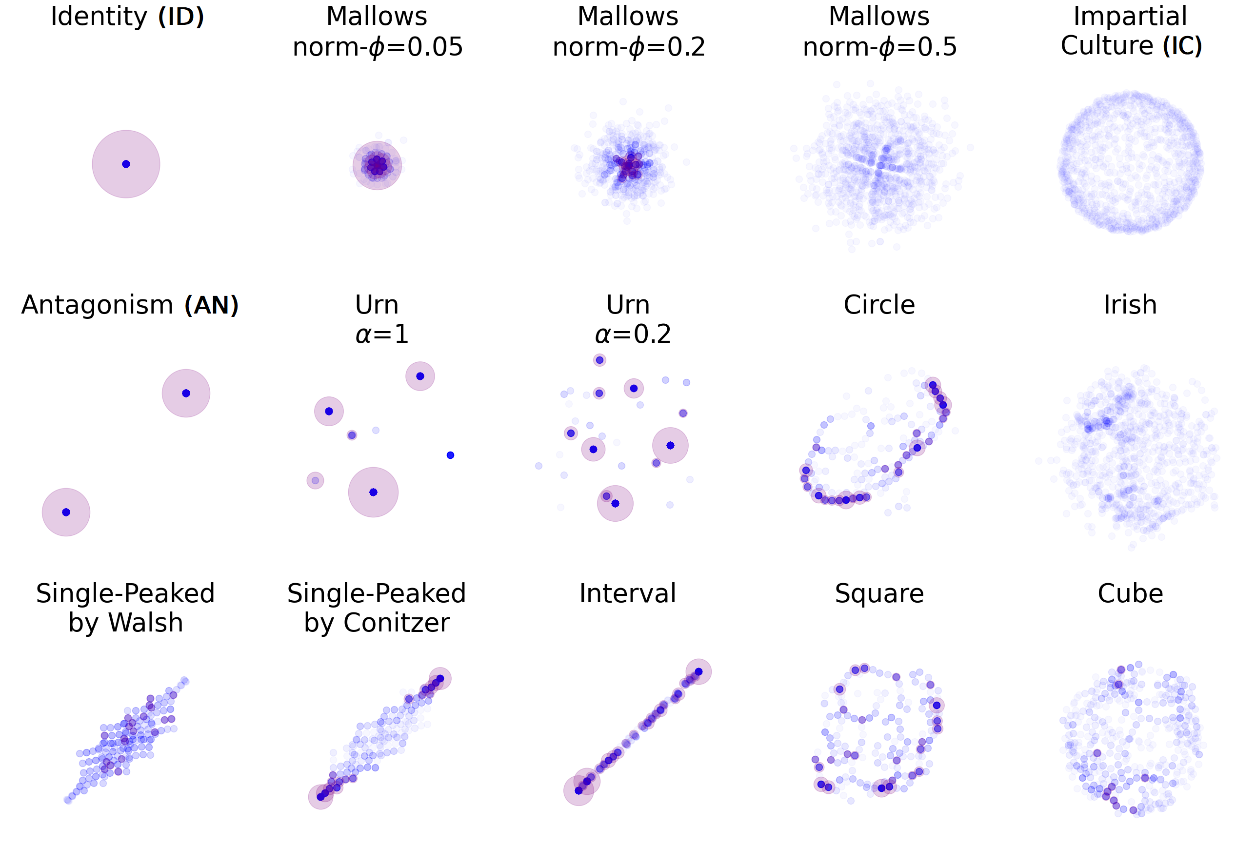
Figure 1: Maps of Preferences (8 candidates, 1000 voters). If there are more than 10 copies of the same vote, we add a purple disc with a radius proportional to the number of voters.

5.2   Model Definitions and Analysis

ID, AN, and IC

We first consider ID, AN, and IC elections (which, for the time being, covers for UN). ID and AN are shown as the first entries of the first two rows in Fig. 1. The former, with 1000 copies of the same vote, presented as a single point with a large purple disc, embodies perfect agreement. The latter, with 500 votes of one type and 500 its reverses, represents a very polarized society, which is well captured by the two faraway points with large discs on its map. Under IC, whose map is the last one in the first row, we see no clear structure except that, of course, there are many pairs of votes at high swap distance (they form the higher-density rim). Yet, for each such pair there are also many votes in between. Hence, it is close to being perfectly diverse.

We do not present UN in our maps because it requires at least $m!$ votes. Indeed, from now on instead of considering UN, we will talk about its approximate variant, $\mathrm{UN}^{*}$, which we generate by sampling votes from its scaled position matrix (see Appendix F for details).

Mallows Model

The Mallows model is parameterized by the central vote $u$ and the dispersion parameter $\phi\in[0,1]$. Votes are generated independently and the probability of generating a vote $v$ is proportional to $\phi^{\mathrm{swap}(u,v)}$. Instead of using the parameter $\phi$ directly, we follow Boehmer et al. (2021) and use its normalized variant, ${{\mathrm{norm}\hbox{-}\phi}}\in[0,1]$, which is internally converted to $\phi$ (see their work for details; with $8$ candidates the conversion is nearly linear). For ${{\mathrm{norm}\hbox{-}\phi}}=1$, the Mallows model is equivalent to IC, for ${{\mathrm{norm}\hbox{-}\phi}}=0$ it is equivalent to ID, and for values in between we get a smooth transition between these extremes (or, between agreement and diversity, to use our high-level notions). We see this in the first row of Fig. 1.

Urn Model

In the Pólya-Eggenberger urn model (Berg, 1985; McCabe-Dansted and Slinko, 2006), we have a parameter of contagion $\alpha\in[0,\infty)$. We start with an urn containing one copy of each possible vote and we repeat the following process $n$ times: We draw a vote from the urn, its copy is included in the election, and the vote, together with $\alpha\cdot m!$ copies, is returned to the urn. For $\alpha=0$ the model is equivalent to IC. The larger is the $\alpha$ value, the stronger is the correlation between the votes.

In Fig. 1, urn elections (shown in the middle of the second row) consist of very few distinct votes. For example, for $\alpha=1$ we only have seven votes, thus this election’s map looks similarly to that for AN—few points with discs. Such elections, with several popular views but without a spectrum of opinions in between, are known as fragmented (Dynes and Tierney, 1994). Hence, we expect their diversity to be small. As $\alpha$ decreases, urn elections become less fragmented.

We upper-bound the expected number of different votes in an urn election with $m$ candidates, $n$ voters (where $n$ is significantly smaller than $m!$), and parameter $\alpha$ by $\sum_{i=1}^{n}\nicefrac{{1}}{{(1+(i-1)\alpha)}}$ (the first vote is always unique, the second one is drawn from the original $m!$ votes from the urn with probability $\nicefrac{{1}}{{(1+\alpha)}}$, and so on; if we draw one of the original votes from the urn it still might be the same as one of the previous ones, but this happens with a small probability when $n$ is significantly smaller than $m!$). For example, for $n=1000$ and $\alpha$ equal to $1$, our formula gives $7.48$. In the literature, authors often use $\alpha=1$ (Erdélyi et al., 2015; Keller et al., 2019; Walsh, 2011), sometimes explicitly noting the strong correlations and modifying the model (Erdélyi et al., 2015). However, smaller values of $\alpha$ also are used (Skowron et al., 2015; McCabe-Dansted and Slinko, 2006). Since $\alpha=1$ gives very particular elections, it should be used consciously.

Single-Peaked Elections

Single-peaked elections (Black, 1958) capture scenarios where voters have a spectrum of opinions between two extremes (like choosing a preferred temperature in a room).

Definition 5 (Black (1958)).

Let $C$ be a set of candidates and let $\rhd$ be an order over $C$, called the societal axis. A vote is single-peaked with respect to $\rhd$ if for each $t\in[|C|]$, its top $t$ candidates form an interval w.r.t. $\rhd$. An election is single-peaked (w.r.t. $\rhd$) if its votes are.

We use the Walsh (Walsh, 2015) and the Conitzer (random peak) models (Conitzer, 2009) of generating single-peaked elections. In the former, we fix the societal axis and choose votes single-peaked with respect to it uniformly at random (so we can look at it as IC over the single-peaked domain). In the Conitzer model we also first fix the axis, and then generate each vote as follows: We choose the top-ranked candidate uniformly at random and fill-in the following positions by choosing either the candidate directly to the left or directly to the right of the already selected ones on the axis, with probability $\nicefrac{{1}}{{2}}$ (at some point we run out of the candidates on one side and then only use the other one).

In Fig. 1, Conitzer and Walsh elections are similar, but the former one has more votes at large swap distance. Indeed, under the Conitzer model, we generate a vote equal to the axis (or its reverse) with probability $\nicefrac{{2}}{{m}}$, which for $m=8$ is $25\%$. Under the Walsh model, this happens with probability $1.5\%$ (it is known there are $2^{m-1}$ different single-peaked votes and Walsh model chooses each of them with equal probability). Hence, our Conitzer elections are more polarized (see the purple discs at the farthest points) than the Walsh ones, and Walsh ones appear to be more in agreement (in other words, the map for the Conitzer election is more similar to that for AN, and the map for Walsh election is more similar to ID).

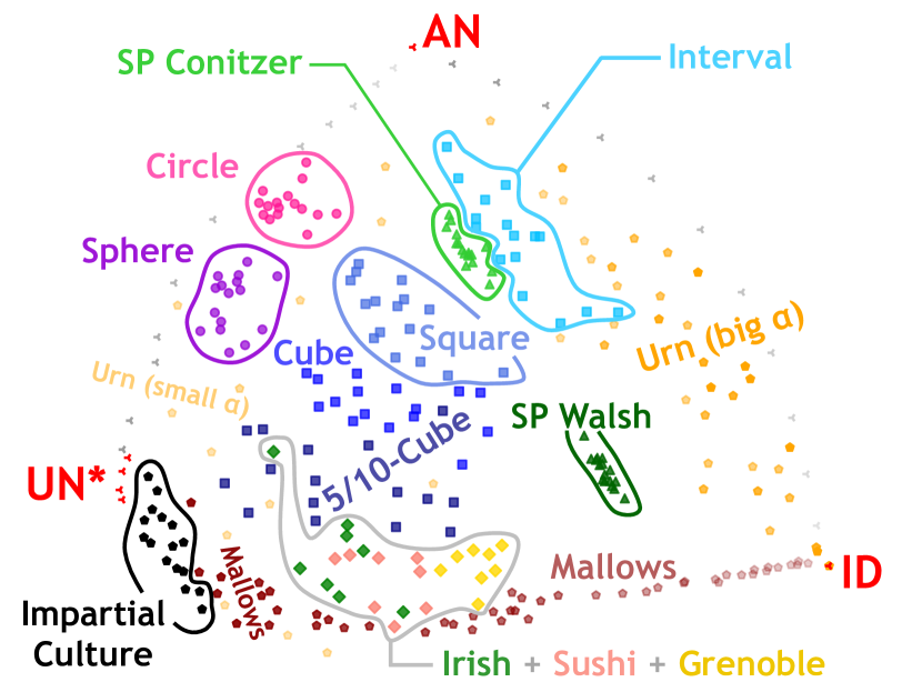
(a) Standard map of elections.

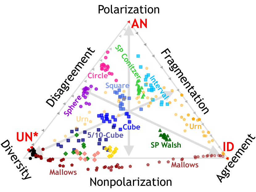
(b) Agreement-diversity map.

Figure 2: Plot (a) shows a map of elections in our dataset obtained using isomorphic swap distance and MDS. Plot (b) presents an affine transformation of a plot where x/y coordinates of the elections are their agreement/diversity indices.

Euclidean Models

In $d$-dimensional Euclidean elections ($d$-Euclidean elections) every candidate and every voter is a point in $\mathbb{R}^{d}$, and a voter prefers candidate $a$ to candidate $b$ if his or her point is closer to that of $a$ than to that of $b$. To generate such elections, we sample the candidate and voter points as follows: (a) In the $d$-Cube model, we sample the points uniformly at random from a $d$-dimensional hypercube $[0,1]^{d}$, and (b) in the Circle and Sphere models we sample them uniformly at random from a circle (embedded in 2D space) and a sphere (embedded in 3D space). We refer to the 1-Cube, 2-Cube, and 3-Cube models as, respectively, the Interval, Square, and Cube models. In Fig. 1, we see that as the dimension increases, the elections become more similar to the IC one (see the transition from the Interval to the Cube one). The Interval election is very similar to those of Conitzer and Walsh, because 1-Euclidean elections are single-peaked. It is also worth noting that the Circle election is quite polarized (we see an increased density of votes on two opposite sides of its map).

Irish and Other Elections Based on Real-Life Data

We also consider elections generated based on real-life data from a 2002 political election in Dublin (Mattei and Walsh, 2013). We treat the full Irish data as a distribution and sample votes from it as from a statistical culture (technical details in Appendix G). The Irish election in Fig. 1 is, in some sense, between the Cube and Mallows ones for ${{\mathrm{norm}\hbox{-}\phi}}=0.5$. Intuitively, we would say that it is quite diverse. In the dataset, we also include Sushi and Grenoble elections, similarly generated using different real-life data (Mattei and Walsh, 2013).

6   Final Experiments and Conclusion

In this section we present the results of computing the agreement, diversity, and polarization indices on our dataset.

6.1   Computing the Indices in Practice

First, we compared three ways of computing $k$-Kemeny distances: the greedy approach, the local search with swap size equal to $1$, and a combined heuristic where we first calculate the greedy solution and then try to improve it using the local search. We ran all three algorithms for all $k\in[96]$ and for every election in our dataset. The complete results are in Appendix K. The conclusion is that the local search and the combined heuristic gave very similar outcomes and both outperformed the greedy approach. Hence, in further computations, we used the former two algorithm and took the smaller of their outputs.

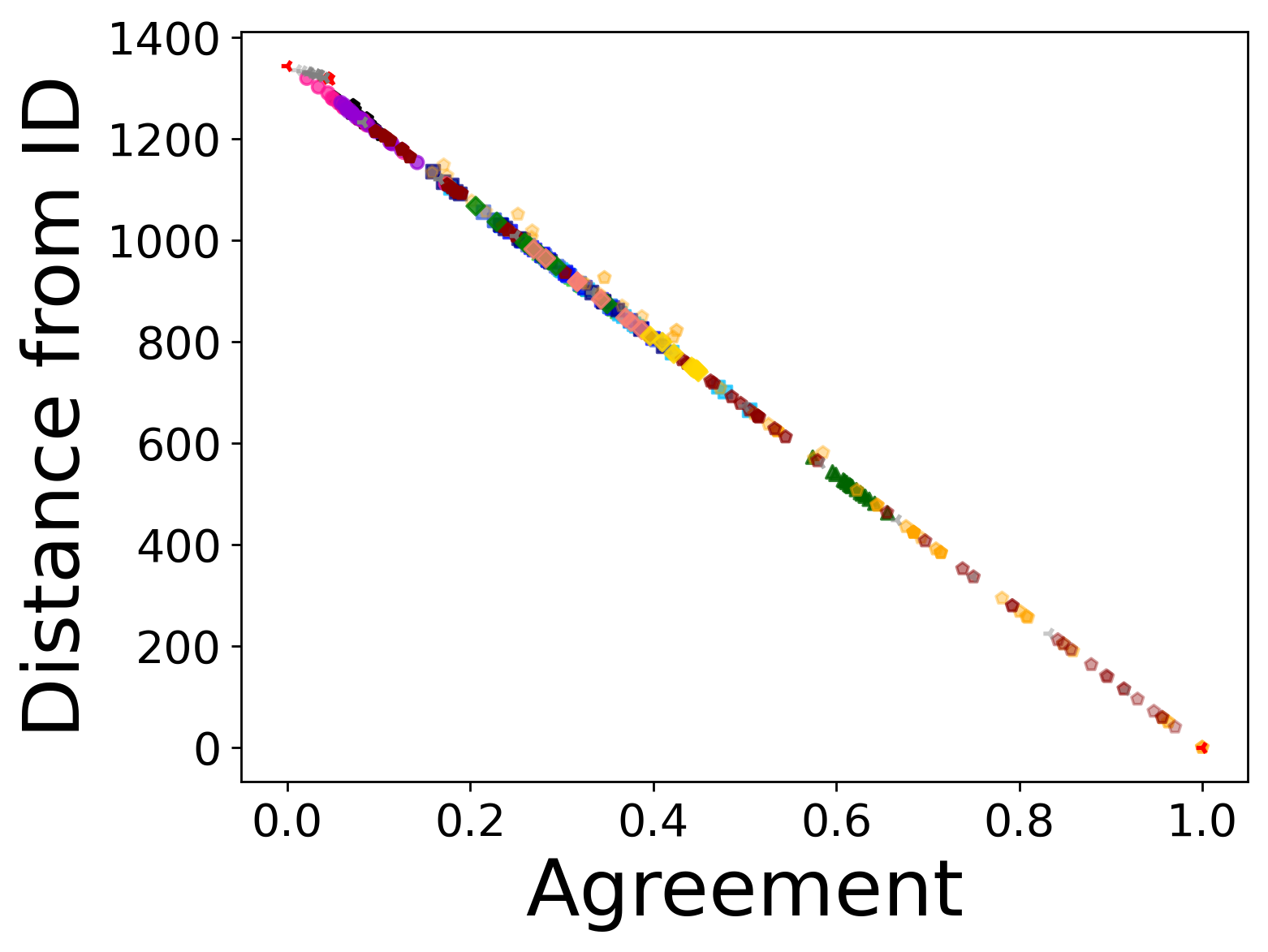
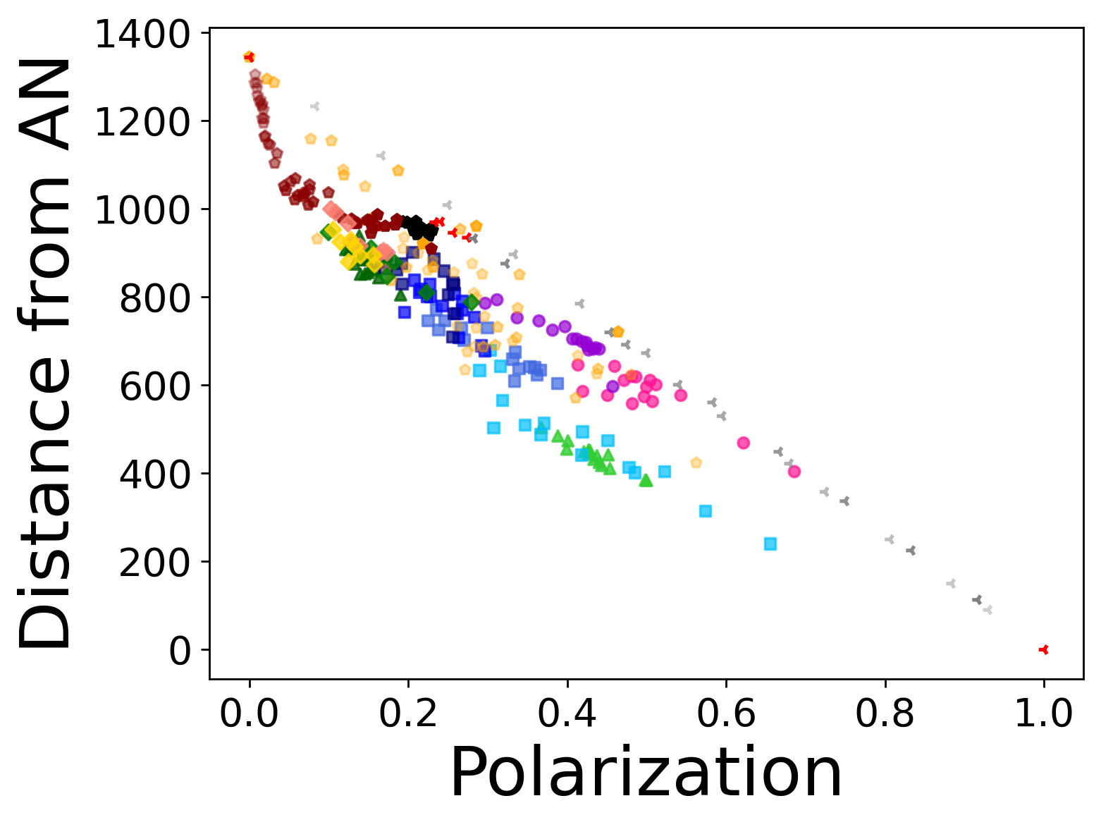
Figure 3: Correlation between our indices and the distance from the respective compass election.

6.2   Understanding the Map via Agreement, Diversity, and Polarization

Using the $\kappa_{k}(E)$ values computed in the preceding experiment, we calculated diversity and polarization indices of all the elections from our datasets, along with their agreement indices (which are straightforward to compute). We illustrate the results in several ways.

First, we consider Fig. 3. In the leftmost plot, each election from our dataset is represented as a dot whose x/y coordinates are the values of the agreement index and the distance from ID, and whose color corresponds to the statistical culture from which it comes (it is the same as in Fig. 2(a), though due to large density of the dots, this only gives a rough idea of the nature of the elections). The next two plots on the right are analogous, except that it regards diversity or polarization and the distance from $\mathrm{UN}^{*}$ or AN, respectively. The Pearson correlation coefficient between each of the three indices and the distance from the respective compass election is below $-0.9$, which means that the correlation is very strong. This is our first indication that the locations on the map of elections, in particular, the one from Fig. 2(a), can be understood in terms of agreement, diversity, and polarization.

Next, for all three pairs of our indices we plotted our dataset in such a way that each election’s x/y coordinates are the values of the respective indices (these plots can be found in Appendix L). We observed that each of these plots resembles the original map from Fig. 2(a). Hence, for the sake of clearer comparison, we took the plot for agreement and diversity indices and, by an affine transformation, converted it to a roughly equilateral triangle spanned between ID, AN, and $\mathrm{UN}^{*}$. Fig. 2(b) presents the result of this operation.

The similarity between Figs. 2(a) and 2(b) is striking as most elections can be found in analogous locations. Even the positions of the outliers in the groups are, at least approximately, preserved. Yet, there are also differences. For example, in Fig. 2(b) elections from most of the statistical cultures are closer to each other, whereas on Fig. 2(a) they are more scattered. Nonetheless, the similarity between these two figures is our second argument for understanding the map in terms of agreement, diversity, and polarization. Specifically, the closer an election is to ID, AN, or $\mathrm{UN}^{*}$, the more agreement, polarization, or diversity it exhibits.

6.3   Validation Against Intuition

Finally, let us check our intuitions from Section 5 against the actually computed values of the indices, as presented on the plot from Fig. 2(b). We make the following observations:

1. We see that Mallows elections indeed progress from ID (for which we use ${{\mathrm{norm}\hbox{-}\phi}}=0$) to IC (for which we use ${{\mathrm{norm}\hbox{-}\phi}}=1$), with intermediate values of ${{\mathrm{norm}\hbox{-}\phi}}$ in between. The model indeed generates elections on the agreement-diversity spectrum.

2. Elections generated using the urn model with large value of $\alpha$ appear on the agreement-polarization line. Indeed, for very large values of $\alpha$ nearly all the votes are identical, but for smaller values we see polarization effects. Finally, as the values of $\alpha$ go toward $0$, the votes become more and more diverse.

3. Walsh elections are closer to agreement (ID) and Conitzer elections are closer to polarization (AN).

4. High-dimensional Cube elections have fairly high diversity. Circle and Sphere elections are between diversity and polarization.

5. Irish elections are between Mallows and high-dimensional Cube elections.

All in all, this confirms our intuitions and expectations.

7   Summary

The starting point of our work was an observation that the measures of diversity and polarization used in computational social choice literature should, rather, be seen as measures of disagreement. We have proposed two new measures and we have argued that they do capture diversity and polarization. On the negative side, our measures are computationally intractable. Hence, finding a measure that would be easy to compute but that would maintain the intuitive appeal of our ones is an interesting research topic.

Appendix

Appendix A Agreement and $\boldsymbol{1}$-Kemeny Distance

In this section, we show the relation between the agreement index and $1$-Kemeny distance. By $\mu$ let us denote the majority relation, which is a (possibly intransitive and not asymmetric) relation on the set of candidates such that for each $a,b\in C$, $a\succeq_{\mu}b$ if and only if $p_{E}(a,b)\geq p_{E}(b,a)$. Let say that the linear order $\lambda$ of candidates is consistent with $\mu$ if $a\succ_{\lambda}b$ implies $a\succeq_{\mu}b$, for every $a,b\in C$. Observe that if an election $E=(C,V)$ does not have a Condorcet cycle, i.e., there is no sequence of candidates $c_{1},\dots,c_{k}\in C$ such that $p_{E}(c_{i},c_{i+1})\geq p_{E}(c_{i+1},c_{i})$, for every $i\in[k-1]$, and $p_{E}(c_{k},c_{1})>p_{E}(c_{1},c_{k})$, then the set of preference orders consistent with $\mu$ is the set of all Kemeny rankings.

The Kendall’s $\tau$ distance can be generalized for any relations. For every linear order $\lambda$ over candidates $C$, we have

$$\tau(\lambda,\mu)=\frac{1}{2}\sum_{a,b\in C}\left(\mathds{1}_{a\succ_{\lambda}b}\cdot\mathds{1}_{a\not\succeq_{\mu}b}+\mathds{1}_{b\succeq_{\mu}a}\cdot\mathds{1}_{b\not\succ_{\lambda}a}\right).$$

In other words, for every pair of candidates $a,b$ for which $a\succ_{\lambda}b$, we count 1, if $b\succeq_{\mu}a$ and $a\not\succeq_{\mu}b$, and $\nicefrac{{1}}{{2}}$, if $b\succeq_{\mu}a$ but also $a\succeq_{\mu}b$. As we show in the following proposition, there is a strict relation between the agreement index and the average Kendall’s $\tau$ distance from all votes to the majority relation.

Proposition 1.

For every election $E=(C,V)$, it holds that

$$A(E)=1-\frac{2\cdot\sum_{v\in V}\tau(v,\mu)}{|V|\cdot\textstyle\binom{|C|}{2}}.$$

Proof.

We split the set of pairs of candidates into two subsets: $A$ containing the pairs with perfect disagreement, and $B$ with the pairs for which some opinion is stronger than the other. Formally, let $A=\{\{a,b\}\subseteq C:p_{E}(a,b)=p_{E}(b,a)\}$ and $B=\{\{a,b\}\subseteq C:p_{E}(a,b)\neq p_{E}(b,a)\}$. Without loss of generality, throughout the proof we assume that for pair $\{a,b\}\in B$ we have $a\succeq_{\mu}b$. Then, by the definition of $\mu$ we get $p_{E}(a,b)>p_{E}(b,a)$ and thus

$$|p_{E}(a,b)-p_{E}(b,a)| =p_{E}(a,b)-p_{E}(b,a)$$

$$=(p_{E}(a,b)+p_{E}(b,a))-2p_{E}(b,a)$$

$$=1-2p_{E}(b,a).$$

Since for $\{a,b\}\in A$ we have $|p_{E}(a,b)-p_{E}(b,a)|=0$, by the definition of the agreement index, we get that

$$A(E) =\frac{\sum_{\{a,b\}\in B}\left(1-2p_{E}(b,a)\right)}{\binom{|C|}{2}}$$

$$=\frac{|B|-2\cdot\sum_{\{a,b\}\in B}\sum_{v\in V}\mathds{1}_{b\succ_{v}a}/|V|}{\binom{|C|}{2}}$$

$$=\frac{|B|}{\binom{|C|}{2}}-2\frac{\sum_{v\in V}\sum_{\{a,b\}\in B}\mathds{1}_{b\succ_{v}a}}{|V|\cdot\binom{|C|}{2}}$$

$$=\frac{|B|}{\binom{|C|}{2}}-2\frac{\sum_{v\in V}\sum_{\{a,b\}\in B}\nicefrac{{1}}{{2}}\mathds{1}_{b\succ_{v}a}+\nicefrac{{1}}{{2}}\mathds{1}_{a\not\succ_{v}b}}{|V|\cdot\binom{|C|}{2}},$$

where the last equation comes from the fact that $\succ_{v}$ is asymmetric, so $\mathds{1}_{b\succ_{v}a}=\mathds{1}_{a\not\succ_{v}b}$. Since for $\{a,b\}\in B$ we have $p_{E}(a,b)>p_{E}(b,a)$, then we know that $\mathds{1}_{a\succeq_{\mu}b}=\mathds{1}_{b\not\succeq_{\mu}a}=1$ and, conversely, $\mathds{1}_{a\not\succeq_{\mu}b}=\mathds{1}_{b\succeq_{\mu}a}=0$. In particular, this means that

/12$$\mathds{1}_{b\succ_{v}a}+\nicefrac{{1}}{{2}}\mathds{1}_{a\not\succ_{v}b} =\nicefrac{{1}}{{2}}\mathds{1}_{b\succ_{v}a}\mathds{1}_{b\not\succeq_{\mu}a}+\nicefrac{{1}}{{2}}\mathds{1}_{a\not\succ_{v}b}\mathds{1}_{a\succeq_{\mu}b}$$

$$+\nicefrac{{1}}{{2}}\mathds{1}_{a\succ_{v}b}\mathds{1}_{a\not\succeq_{\mu}b}+\nicefrac{{1}}{{2}}\mathds{1}_{b\not\succ_{v}a}\mathds{1}_{b\succeq_{\mu}a},$$

which we denote as $\tau_{a,b}(v.\mu)$. Then, we have that

$$A(E)=\frac{|B|}{\binom{|C|}{2}}-2\frac{\sum_{v\in V}\sum_{\{a,b\}\in B}\tau_{a,b}(v,\mu)}{|V|\cdot\binom{|C|}{2}}.$$ (1)

Now, let us consider a pair of candidates $\{a,b\}\in A$. Observe that independently whether $a\succ_{v}b$ or $b\succ_{v}a$ we have that

$$\tau_{a,b}(v,\mu)=\hskip 3.0pt \mathds{1}_{b\succ_{v}a}\cdot 0+\nicefrac{{1}}{{2}}\mathds{1}_{a\not\succ_{v}b}\cdot 1$$ /12

$$+\hskip 3.0pt \mathds{1}_{a\succ_{v}b}\cdot 0+\nicefrac{{1}}{{2}}\mathds{1}_{b\not\succ_{v}a}\cdot 1=\nicefrac{{1}}{{2}}.$$ /12

Therefore, summing for all voters and pairs of candidates in set $A$, we obtain

$$\textstyle\sum_{v\in V}\sum_{\{a,b\}\in A}\tau_{a,b}(v,\mu)=\nicefrac{{1}}{{2}}|A|\cdot|V|.$$

We can rearrange this equation and divide by $\nicefrac{{1}}{{2}}|V|\binom{|C|}{2}$, to get

$$0=\frac{|A|}{\binom{|C|}{2}}-2\frac{\sum_{v\in V}\sum_{\{a,b\}\in A}\tau_{a,b}(v,\mu)}{|V|\cdot\binom{|C|}{2}}.$$

Combining this we equation (1) we obtain

$$A(E) =1-2\frac{\textstyle\sum_{v\in V}\sum_{\{a,b\}\subseteq C}\tau_{a,b}(v,\mu)}{|V|\cdot\textstyle\binom{|C|}{2}}$$

$$=1-\frac{2\cdot\textstyle\sum_{v\in V}\tau(v,\mu)}{|V|\cdot\textstyle\binom{|C|}{2}}.$$

∎

Since in elections without a Condorcet cycles every Kemeny ranking is consistent with $\mu$, we get that in such elections there is a strict relation between the agreement index and $1$-Kemeny distance.

Corollary 3.

For every election $E=(C,V)$ without a Condorcet cycle, it holds that

$$A(E)=1-2\cdot\kappa_{1}(E)/\left(|V|\cdot\textstyle\binom{|C|}{2}\right).$$

Appendix B Proof of Theorem 1

For a given instance $I=(E=(C,V),k)$ a feasible solution for $k$-Kemeny Among Votes is also a feasible solution to $k$-Kemeny. Let $\mu_{k}(E)$ be the optimum value of $k$-Kemeny Among Votes on $I$ and $\kappa_{k}(E)$ be the optimum value of $k$-Kemeny on $I$. In order to show the theorem statement it is enough to show that $\mu_{k}(E)\leq 2\kappa_{k}(E)$.

Let $\Lambda=\{\lambda_{1},\dots,\lambda_{k}\}$ be an optimum solution for $k$-Kemeny Among Votes and $\Gamma=\{\gamma_{1},\dots,\gamma_{k}\}$ be an optimum solution for $k$-Kemeny. Let $v(x)\in V$ be a voter that is closest to some ranking $x$ and $v(\Gamma)=\{v(\gamma):\gamma\in\Gamma\}$. Let $\gamma(x)\in\Gamma$ be a ranking from $\Gamma$ that is closest to some ranking $x$. We define $\mathrm{swap}(v,X)=\min_{x\in X}\mathrm{swap}(v,x)$. We have

$$\mu_{k}(E) =\sum_{v\in V}\mathrm{swap}(v,\Lambda)$$

$$\leq\sum_{v\in V}\mathrm{swap}(v,v(\Gamma))$$

$$\leq\sum_{v\in V}\Big{(}\mathrm{swap}(v,\gamma(v))+\mathrm{swap}(\gamma(v),v(\gamma(v)))\Big{)}$$

$$\leq 2\cdot\sum_{v\in V}\mathrm{swap}(v,\gamma(v))=2\kappa_{k}(E).$$

where the first inequality holds because of optimality of $\Lambda$ restricted to votes and the second inequality is due to the triangle inequality. The third inequality follows from $\mathrm{swap}(\gamma(v),v(\gamma(v)))\leq\mathrm{swap}(\gamma(v),v)$, which expresses that for some vote $v\in V$, its distance to the closest ranking $\gamma(v)$ from $\Gamma$ is at least as large as the distance between $\gamma(v)$ and a vote closest to it. This finishes the proof.

Appendix C Proof of Theorem 2

Let us fix some $\epsilon>0$.

We consider every possible subset of votes as a cluster; there are $2^{n}$ of them. First, our algorithm runs a PTAS designed for $1$-Kemeny [Kenyon-Mathieu and Schudy, 2007] for every possible cluster and store the result. This gives us an $(1+\epsilon)$-approximate solution for every cluster separately.

Second, our algorithm guesses a $k$-clustering $\{V_{1},V_{2},\ldots,V_{k}\}$ of votes. Then, for each cluster in the clustering, we take an $(1+\epsilon)$-approximate solution to $1$-Kemeny (which was computed in the first step) and store it. The algorithm repeats this procedure for each of $k^{n}$ possible clusterings and outputs the smallest computed distance.

It is clear that an optimum solution corresponds to one of the $k$-clusterings, say $K$, analyzed by the algorithm in the second step. Moreover, in each cluster of $K$ the solution returned by the algorithm is a $(1+\epsilon)$-approximation of the optimum solution of the cluster under consideration. Hence, eventually, the algorithm returns a $k$-Kemeny solution that costs at most a multiplicative factor $1+\epsilon$ more than the optimum one, as claimed.

Regarding the running time, note that $k<n$; otherwise, the set of votes gives a solution of cost $0$. The algorithm computes a solution for $2^{n}$ many clusters (each in polynomial time) and considers $k^{n}\leq n^{n}$ many clusterings (each in polynomial time), so the running time is FPT w.r.t. $n$, namely $n^{n}\cdot\operatorname{poly}(n,m)$.

Appendix D Proof of Theorem 3

In the main text we provided the construction of the reduction. Here we prove its correctness.

First, let us assume that there is some (partial) cover ${\mathcal{R}}\subseteq{\mathcal{S}},|{\mathcal{R}}|=K$ such that $|\bigcup_{S\in{\mathcal{R}}}S|\geq T$. We claim that the set $\Lambda=\{\succ_{v_{j}}:S_{j}\in{\mathcal{R}}\}$ of $k$ rankings has the $k$-Kemeny distance at most $D$.

For every (copy of) set-voter $v_{j}$ such that $S_{j}\in{\mathcal{R}}$, we have $\mathrm{swap}(v_{j},\Lambda)\leq\mathrm{swap}(v_{j},v_{j})=0$ and for the remaining $L(M-K)$ set-voters the distance to $\Lambda$ equals $2$. Hence, set-voters realize the distance equal to the first term in the definition of $D$.

Now, we calculate the distance realized by element-voters. For each element-voter $e_{i}$, representing element $x_{i}$ that is not covered by ${\mathcal{R}}$, its swap distance $\mathrm{swap}(e_{i},\Lambda)$ can be computed as follows. Starting from the distance being $0$, we add one for each set in which $x_{i}$ is included and we add $3$ because of the pivot-candidates. Furthermore, we increase the distance by one once more, due to the following. For every vote $v_{j}\in\Lambda$ (recall that in $v_{j}$ candidate $d_{S_{j}}$ is preferred to $c_{S_{j}}$), we have that in vote $e_{i}$ candidate $c_{S_{j}}$ is preferred to $d_{S_{j}}$, since $x_{i}$ is not covered. So, formally, for an element-voter $e_{i}$ that represents an element $x_{i}$ not covered by ${\mathcal{R}}$, we obtain the following formula:

$$\mathrm{swap}(e_{i},\Lambda)=|\{S\in{\mathcal{S}}:x_{i}\in S\}|+3+1.$$

If, however, element $x_{i}$ is covered by some set, say $S_{j}$, in ${\mathcal{R}}$, then candidates $c_{S_{j}}$ and $d_{S_{j}}$ are in the same order in $e_{i}$ and $v_{j}$ and $v_{j}\in\Lambda$. Hence, we should decrease the computed distance by two. By one, due to the fact that, we added one for each set in $x_{i}$ is included; hence we also assumed that the order of $c_{S_{j}}$ and $d_{S_{j}}$ is reversed in $e_{i}$ and $v_{i}$. By another one because also the last summand of the aforementioned formula came from the (now false) assumption there is no vote in $\Lambda$ for which  $c_{S_{j}}$ and $d_{S_{j}}$ are in the same order in $e_{i}$ and $v_{i}$. Since we computed their inversion in the first part of the formula. Eventually, introducing the indicator function $\operatorname{\mathbbm{1}}[\Phi]$ such that $\operatorname{\mathbbm{1}}[\Phi]=1$ if $\Phi$ is true, and $\operatorname{\mathbbm{1}}[\Phi]=0$ otherwise, formally the sought $\mathrm{swap}(e_{i},\Lambda)$ is

$$\mathrm{swap}(e_{i},\Lambda)=|\{S\in{\mathcal{S}}:x_{i}\in S\}|+4-2\cdot\operatorname{\mathbbm{1}}[x_{i}\in\bigcup_{S\in{\mathcal{R}}}S].$$

It means that the distance realized by element-voters is equal to

$$\sum_{i\in[N]}\mathrm{swap}(e_{i},\Lambda) =\sum_{j\in[M]}|S_{j}|+4N-2\cdot\Big{|}\bigcup_{S\in{\mathcal{R}}}S\Big{|}$$

$$\leq\sum_{j\in[M]}|S_{j}|+4N-2T.$$

In total, $\mathrm{swap}(V,\Lambda)\leq D$, as required.

Now, let us assume that there is $\Lambda\subseteq\{\succ_{v}:v\in V\},|\Lambda|=k$ such that $\mathrm{swap}(V,\Lambda)\leq D$.

First of all, we observe that $\Lambda$ may contain only rankings of set-voters. Let us assume, by contradiction, that there is an element-voter in $\Lambda$. It means that at most $L(k-1)$ set-voters realize the swap distance $0$. Furthermore, at least $L(M-k+1)$ set-voters realize the swap distance at least $2$ (it is exactly $2$ when the closest ranking comes from a set-vote, and it is at least $3$ when the closest ranking comes from an element-vote). Hence, we would have $\mathrm{swap}(V,\Lambda)\geq 2L(M-k+1)>2L(M-K)+NM+4N\geq D$, which is a contradiction with $\mathrm{swap}(V,\Lambda)\leq D.$

Using the same calculation as in the previous paragraph, we can conclude that $\Lambda$ does not contain two copies of the same set-voter. Because of that, we can define ${\mathcal{R}}\subseteq{\mathcal{S}}$ containing exactly $k=K$ subsets corresponding to votes from $\Lambda$, i.e., ${\mathcal{R}}=\{S_{j}:\ \succ_{v_{j}}\in\Lambda\}$.

We will show that ${\mathcal{R}}$ covers at least $T$ elements. Let us assume, by contradiction, that ${\mathcal{R}}$ covers at most $T-1$ elements. Then we would have:

$$\mathrm{swap}(V,\Lambda) =2L(M-K)+\sum_{j\in[M]}|S_{j}|+4N-2\cdot\Big{|}\bigcup_{S\in{\mathcal{R}}}S\Big{|}$$

$$\geq 2L(M-K)+\sum_{j\in[M]}|S_{j}|+4N-2(T-1)$$

$$=D+2,$$

which is a contradiction with $\mathrm{swap}(V,\Lambda)\leq D$.

Appendix E Propositions from Theorem 3

Let us define $M=\max_{v,u\in V}\mathrm{swap}(v,u)$, i.e., the maximum distance between votes. The value of $M$ is small in instances with similar votes. Unfortunately, small values of $M$ do not make the problem easy.

Proposition 2.

$k$-Kemeny Among Votes is $\mathrm{W}$[1]-hard when parameterized by $k+M$.

Proof.

It is known that Max $K$-Cover is W[1]-hard w.r.t. $K+f$ [Bonnet et al., 2016], where $f$ is the maximum frequency of an element, i.e., $f=\max_{i\in[N]}|\{S_{j}\in{\mathcal{S}}:x_{i}\in S_{j}\}|$. We can observe that $M\leq 2f+4$ in the reduction given in the proof of Theorem 3 hence we obtain the proposition statement. ∎

By adapting results regarding Max $K$-Cover [Sornat et al., 2022, Observation 7], we also obtain the following bound that uses the Strong Exponential Time Hypothesis (SETH).

Proposition 3.

There is no $1.4^{m}\cdot\operatorname{poly}(n,m)$-time algorithm for $k$-Kemeny Among Votes, where $m$ is the number of candidates and $n$ is the number of voters, unless SETH fails.

Proof.

Let us assume, by contradiction, that there is a $1.4^{m}\cdot\operatorname{poly}(n,m)$-time algorithm for $k$-Kemeny Among Votes. We take an instance of Max $K$-Cover and reduce it (in $\operatorname{poly}(N,M)$ time) to $k$-Kemeny Among Votes using the reduction from the proof of Theorem 3. We solve the obtained instance of $k$-Kemeny Among Votes in time $1.4^{m}\cdot\operatorname{poly}(n,m)$ and we output the same response to Max $K$-Cover. Due to Theorem 3, we obtained a correct response to the instance of Max $K$-Cover. Recall that $m=2M+3$ and $n=N(M^{2}+4M+1)$. Therefore, the running time of our algorithm for Max $K$-Cover is at most $1.4^{m}\cdot\operatorname{poly}(n,m)\cdot\operatorname{poly}(N,M)\leq 1.4^{2M+3}\cdot\operatorname{poly}(N,M)\leq 1.96^{M}\cdot\operatorname{poly}(N,M)$. This would show that SETH is false because under SETH Max $K$-Cover has no $1.99^{M}\cdot\operatorname{poly}(N,M)$ time algorithm [Sornat et al., 2022, Observation 7]. ∎

On the other hand, $k$-Kemeny Among Votes (and $k$-Kemeny) is FPT w.r.t. $m$ by a brute-force evaluation of all $k$-size subsets of $m!$ possible linear orders as a solution, each in polynomial time. Hence, the running time is $\binom{m!}{k}\cdot\operatorname{poly}(n,m)\leq 2^{m!}\cdot\operatorname{poly}(n,m)\leq 2^{m^{m}}\cdot\operatorname{poly}(n,m)$. This is a double-exponential dependence. An open question is to provide a single-exponential time algorithm.

Table 1: The ingredients of the standard dataset.

model	variants/parameters	#elcs
Impartial Culture		16
normalized Mallows	$\phi\in\textrm{unif. over }[0,1]$	48
urn model	$\alpha\in\Gamma(0.8)$	48
single-peaked (Conitzer)		16
single-peaked (Walsh)		16
1-cube (Interval)	uniform interval	16
2-cube (Square)	uniform square	16
3-cube (Cube)	uniform cube	16
5-cube	uniform 5D-cube	8
10-cube	uniform 10D-cube	8
circle	circle in 2D	16
sphere	sphere in 3D	16
Irish dataset		8
Sushi dataset		8
Grenoble dataset		8
uniformity ($\mathrm{UN}^{*}$)		4
identity (ID)		1
antagonism (AN)		1
ID-AN mixture	AN fractions: $\nicefrac{{1}}{{12}}\ldots\nicefrac{{11}}{{12}}$	11
AN-$\mathrm{UN}^{*}$ mixture	$\mathrm{UN}^{*}$ fractions: $\nicefrac{{1}}{{12}}\ldots\nicefrac{{11}}{{12}}$	11

Appendix F Standard Dataset Composition

The map of elections from Fig. 2(a) consists of elections from various statistical cultures. In Table 1 we specify how many elections come from each culture and how their parameters were chosen. From now on, we will call this collection of elections (i.e., the elections depicted in Fig. 2(a)) as the standard dataset, to distinguish it from the extended dataset and the Mallows dataset presented in the following sections. In what follows, we describe how we generate elections that were not covered in Section 5 (or Appendix G).

Before we begin, let us describe a general technique that is sampling elections from a position matrix. A position matrix [Szufa et al., 2020, Boehmer et al., 2021] is an integer $m\times m$ matrix, in which the values of each row and each column sum up to some constant $n\in\mathbb{N}$. An election, $E=(C,V)$, realizes a given position matrix $X$, if $|C|=m$, $|V|=n$, and for every $i,j\in[m]$, the value in $i$-th row and $j$-th column of matrix $X$, i.e., $X_{i,j}$, is equal to the number of voters in $V$ that ranks the $j$-th candidate at the $i$-th position (note that one position matrix can be realized by multiple elections). For example, a position matrix realizing UN election with $m$ candidates, is an $m\times m$ matrix with each element equal to $(m-1)!$. Boehmer et al. [2023], provide a technique to sample elections realizing given position matrix $X$, which starts from an empty election without any votes, and then, iteratively:

1. finds a vote $v$ that can belong to an election realizing $X$,

2. adds $v$ to the election, and then

3. updates the values of matrix $X$ (by subtracting one from $X_{i,j}$ for every $j\in[m]$ and $i$ being the position of $j$-th candidate according to vote $v$),

until $X$ is a zero matrix. We note that this procedure returns every election realizing given matrix with positive probability, but the exact distribution we obtain is unknown (Boehmer et al. [2023] argue that obtaining a P-time uniform sampler is challenging). We use this sampling technique to generate $\mathrm{UN}^{*}$ and AN-$\mathrm{UN}^{*}$ mixture elections.

UN*

To generate $\mathrm{UN}^{*}$ elections, we sample an election realizing an $8\times 8$ position matrix in which every element is equal to $12$.

ID-AN mixture.

Elections from ID-AN mixture model with AN share $i\in\{\nicefrac{{1}}{{12}},\dots,\nicefrac{{11}}{{12}}\}$ come from merging AN election with $96i$ voters and ID election with $96(1-i)$ voters. Hence, we have $96-48i$ voters with a given preference order and $48i$ voters with exactly opposing views.

AN-UN* mixture.

Elections from AN-$\mathrm{UN}^{*}$ mixture model with $\mathrm{UN}^{*}$ share $i\in\{\nicefrac{{1}}{{12}},\dots,\nicefrac{{11}}{{12}}\}$ come from merging $\mathrm{UN}^{*}$ election with $96i$ voters and AN election with $96(1-i)$ voters. Hence, we have $48(1-i)$ voters with a given preference order, $48(1-i)$ voters with exactly opposing views, and on top of that we add $96i$ voters that we get by sampling election realizing $8\times 8$ matrix in which every element is equal $12i$.

Appendix G Preprocessing of Real-life Data

Grenoble.

In the Grenoble field experiment, $760$ people were asked to place $11$ candidates on the $[0,1]$ line. The higher the value, the more a given candidate is liked by a voter. We converted each participant’s line preference into ordinal ranking, by choosing the candidate being closest to one as a first choice, the second closest to one as a second choice and so on.

Sushi.

In the survey about Sushi there were $5000$ participants and $10$ different types of sushi (i.e., candidates). The original data consists of full ordinal rankings without ties.

Irish.

In the election held in Dublin North constituency, there were $43942$ voters and $12$ candidates. In the original data many votes were incomplete, hence, we filled them using the same procedure as Boehmer et al. [2021], in order to obtain complete preference orders.

Sampling procedure.

We decided to conduct experiments with $8$ candidates, hence, for all three dataset we selected $8$ candidates having the highest Borda score. We treat all three datasets as statistical cultures. To sample an election from a given dataset, we simply sample a given number of votes (in our case $1000$) uniformly at random (sequentially with returning).

Appendix H Extended Dataset

In this section, we introduce our extended dataset. This dataset consists of all 292 elections from the standard dataset and 74 new elections generated using 4 additional statistical cultures (single-peaked on a circle, single-crossing, group-separable balanced, and group separable caterpillar) and 2 special models ($\alpha$-stratification and ID-$\mathrm{ST}^{*}$ mixture). The exact composition of the extended dataset is presented in Table 2. In what follows we describe each new culture and model.

We present also map of preferences for elections from these cultures in Fig. 4 (some additional maps for cultures and models already appearing in the standard dataset are also included). In order to obtain maps of preferences more representative for their models, we generated elections with 1000 voters instead of 96 (but we present also the version with 96 voters in Appendix J). Finally, a map of elections generated in the same way as that in Fig. 2(a), but for elections in the extended dataset is presented in Fig. 5.

Table 2: The ingredients of the extended dataset (elections not appearing in the standard dataset are in boldface).

model	variants/parameters	#elcs
Impartial Culture		16
normalized Mallows	$\phi\in\textrm{unif. over }[0,1]$	48
urn model	$\alpha\in\Gamma(0.8)$	48
single-peaked (Conitzer)		16
single-peaked (Walsh)		16
single-peaked on a circle		16
single-crossing		16
group-separable	balanced	16
group-separable	caterpillar	16
1-cube (Interval)	uniform interval	16
2-cube (Square)	uniform square	16
3-cube (Cube)	uniform cube	16
5-cube	uniform 5D-cube	8
10-cube	uniform 10D-cube	8
circle	circle in 2D	16
sphere	sphere in 3D	16
Irish dataset		8
Sushi dataset		8
Grenoble dataset		8
uniformity ($\mathrm{UN}^{*}$)		4
$\mathbf{\nicefrac{{\mathbf{1}}}{{2}}}$-stratification ($\mathbf{ST^{*}}$)		4
identity (ID)		1
antagonism (AN)		1
$\boldsymbol{\alpha}$-stratification	$\alpha\in\{\nicefrac{{1}}{{8}},\nicefrac{{2}}{{8}},\nicefrac{{3}}{{8}}\}$	3
ID-AN mixture	AN share: $\nicefrac{{1}}{{12}}\ldots\nicefrac{{11}}{{12}}$	11
AN-$\mathrm{UN}^{*}$ mixture	$\mathrm{UN}^{*}$ share: $\nicefrac{{1}}{{12}}\ldots\nicefrac{{11}}{{12}}$	11
ID-$\mathbf{ST^{*}}$ mixture	no. blocks: $3$, $4$, $6$	3

Single-Peaked On a Cycle Elections (SPOC)

Elections single-peaked on a circle [Peters and Lackner, 2020] are analogous to single-peaked ones, except that the societal axis is cyclic (so a vote is SPOC with respect to axis $\rhd$ if for every $t\in[m]$ its $t$ top-ranked candidates either form an interval with respect to $\rhd$ or a complement of an interval; an election is SPOC if there is an axis with respect to which all its votes are SPOC). Such preferences occur, e.g., when choosing a virtual meeting time and voters are in different time zones. We generate SPOC elections by choosing SPOC votes uniformly at random (for SPOC, this is equivalent to using the Conitzer approach). The shape of the SPOC election in Fig. 4 naturally corresponds to the cyclic nature of the axis.

Single-Crossing Elections

Single-crossingness captures a similar idea as single-peakedness, but based on ordering the voters.

Definition 6 (Mirrlees [1971], Roberts [1977]).

An election is single-crossing if it is possible to order the voters so that for each two candidates $a$ and $b$ either every voter who prefers $a$ to $b$ comes before every voter who prefers $b$ to $a$, or the other way round.

We generate single-crossing elections using the approach of Szufa et al. [2020]. First, we generate a single-crossing domain, i.e., a set of votes such that any multisubset of them is single-crossing. Then we draw the required number of votes from the domain, uniformly at random. To obtain the domain (for candidate set $C=\{c_{1},\ldots,c_{m}\}$), we first generate vote $v_{1}\colon c_{1}\succ c_{2}\succ\cdots\succ c_{m}$, and for each $i\in[n]\setminus\{1\}$ we obtain $v_{i}$ by copying $v_{i-1}$ and swapping a random pair of adjacent candidates, but so that $v_{1},\ldots,v_{i}$ are single-crossing (for this order). Unfortunately, this is not a uniform sampling procedure (obtaining a $\mathrm{P}$-time one is an open problem).

The map of a single-crossing election in Fig. 4 shows a linear spectrum of opinions, from one vote to its reverse. Indeed, the consecutive votes in the single-crossing domain differ by single swaps, and this is exactly what we see.

Group-Separable Elections

We define group-separable elections following the tree-based approach of Karpov [2019] (see also the work of Elkind et al. [2012]) rather than the original one [Inada, 1964, 1969]. The idea is that candidates have features (organized hierarchically in a tree) and voters have preferences over these features.

Let $C$ be a candidate set and let ${\mathcal{T}}$ be a rooted, ordered tree whose each leaf is labeled with a unique candidate (intuitively, each internal node represents a feature and a candidate has the features that form its path to the root). A vote is consistent with ${\mathcal{T}}$ if we can obtain it by reading the leaves of ${\mathcal{T}}$ from left to right after, possibly, reversing the order of some nodes’ children.

Definition 7.

An election is group-separable if there is a rooted, ordered tree ${\mathcal{T}}$ whose each leaf is associated with a unique candidate, such that each vote of the election is consistent with ${\mathcal{T}}$.

For a tree ${\mathcal{T}}$, we generate consistent elections uniformly at random: We obtain each vote by, first, reversing the order of each internal node’s children with probability $\nicefrac{{1}}{{2}}$ and, then, reading off the candidates from the leaves left to right. We focus on complete binary trees (where every level except, possibly, the last one is completely filled) and on binary caterpillar trees (where each internal node has two children, of which at least one is a leaf). These trees give, respectively, balanced and caterpillar group-separable elections.

In Fig. 4, the group-separable elections are very distinct from all the other ones and reflect the structures of their trees. While it seems that they had only a few distinct votes, this is not the case (it is known that for a binary tree with $m$ candidates, there are $2^{m-1}$ consistent votes), but many of their votes are similar; they are less fragmented than they appear, but there is a level of polarization (especially in the balanced ones).

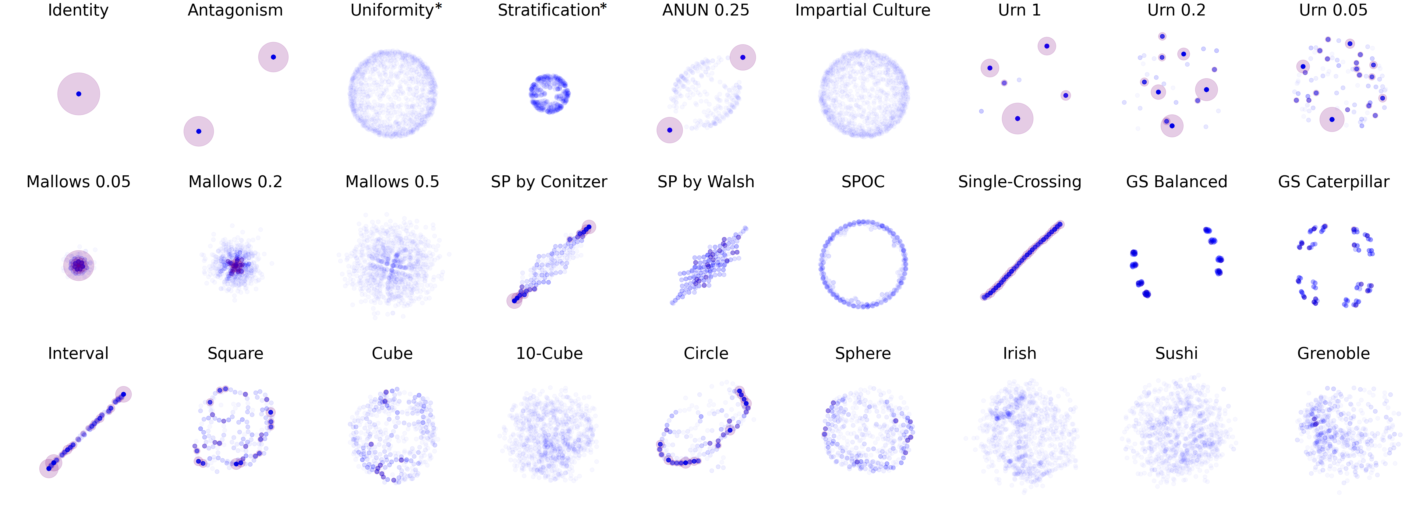
Figure 4: Maps of Preferences (8 candidates, 1000 voters).

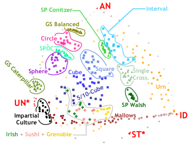
Figure 5: A map of elections in the extended dataset obtained using isomorphic swap distance and MDS.

Stratification

In $\alpha$-stratification election ($\alpha$-ST) [Boehmer et al., 2021] the set of candidates, $C$, is partitioned into two subsets $D_{1}$ and $D_{2}$, where the first group contains $\alpha$ fraction of candidates, i.e., $|D_{1}|/|C|=\alpha$ (if no $\alpha$ is given it is assumed that $\alpha=\nicefrac{{1}}{{2}}$). Intuitively, in such election all voters agree that candidates $D_{1}$ are better than $D_{2}$, but all orderings of candidates inside the subsets are equally represented. Hence, every possible vote that ranks all candidates in $D_{1}$ above all candidates in $D_{2}$ (but with arbitrary orderings inside subsets) appears exactly the same number of times. However, this means that $\alpha$-stratification election requires at least $(\alpha|C|)!\cdot((1-\alpha)|C|)!$ voters. To cope with this problem, we consider approximated $\alpha$-stratification elections ($\alpha$-$\mathrm{ST}^{*}$) that we generate using the same sampling technique as described in Appendix F, but whit different matrices. In particular, for $\alpha\in\{\nicefrac{{1}}{{8}},\nicefrac{{1}}{{4}},\nicefrac{{3}}{{8}},\nicefrac{{1}}{{2}}\}$ we generate $\alpha$-$\mathrm{ST}^{*}$ election by sampling an election realizing the matrix $X^{\alpha}$ given as follows:

$$X^{\nicefrac{{1}}{{2}}} =\left[\begin{array}[]{cccccccc}24&24&24&24&&&&\\ 24&24&24&24&&&&\\ 24&24&24&24&&&&\\ 24&24&24&24&&&&\\ &&&&24&24&24&24\\ &&&&24&24&24&24\\ &&&&24&24&24&24\\ &&&&24&24&24&24\end{array}\right],$$

$$X^{\nicefrac{{3}}{{8}}} =\left[\begin{array}[]{cccccccc}32&32&32&&&&&\\ 32&32&32&&&&&\\ 32&32&32&&&&&\\ &&&20&19&19&19&19\\ &&&19&20&19&19&19\\ &&&19&19&20&19&19\\ &&&19&19&19&20&19\\ &&&19&19&19&19&20\end{array}\right],$$

$$X^{\nicefrac{{2}}{{8}}} =\left[\begin{array}[]{cccccccc}48&48&&&&&&\\ 48&48&&&&&&\\ &&16&16&16&16&16&16\\ &&16&16&16&16&16&16\\ &&16&16&16&16&16&16\\ &&16&16&16&16&16&16\\ &&16&16&16&16&16&16\\ &&16&16&16&16&16&16\end{array}\right],$$

$$X^{\nicefrac{{1}}{{8}}} =\left[\begin{array}[]{cccccccc}96&&&&&&&\\ &14&14&14&14&14&13&13\\ &13&14&14&14&14&14&13\\ &13&13&14&14&14&14&14\\ &14&13&13&14&14&14&14\\ &14&14&13&13&14&14&14\\ &14&14&14&13&13&14&14\\ &14&14&14&14&13&13&14\end{array}\right].$$

The map for $\mathrm{ST}^{*}$ election in Fig. 4 resembles a bit the map for Mallows elections, and it also lands between ID and IC. This is expected: In these elections there is some agreement between the voters (they distinguish the stronger group from the weaker one) but there is also room for diversity.

ID-ST* mixture.

Finally, we consider elections that capture a transition from $\mathrm{ST}^{*}$ to ID. Specifically, instead of dividing candidates into two subsets (aka blocks) on ordering of which the voters agree we divide the candidates in $k$ blocks for some $2\leq k\leq|C|$. If we choose $k=2$ we get a standard stratification election and for $k=|C|$ we get identity. In the extended dataset, we included one such election for each $k\in\{3,4,6\}$. Again, they were obtained by sampling (using procedure described in Appendix F) from the position matrix $X^{k}$ given as follows:

$$X^{3} =\left[\begin{array}[]{cccccccc}48&48&&&&&&\\ 48&48&&&&&&\\ &&32&32&32&&&\\ &&32&32&32&&&\\ &&32&32&32&&&\\ &&&&&32&32&32\\ &&&&&32&32&32\\ &&&&&32&32&32\end{array}\right],$$

$$X^{4} =\left[\begin{array}[]{cccccccc}48&48&&&&&&\\ 48&48&&&&&&\\ &&48&48&&&&\\ &&48&48&&&&\\ &&&&48&48&&\\ &&&&48&48&&\\ &&&&&&48&48\\ &&&&&&48&48\\ \end{array}\right],$$

$$X^{6} =\left[\begin{array}[]{cccccccc}96&&&&&&&\\ &48&48&&&&&\\ &48&48&&&&&\\ &&&48&48&&&\\ &&&48&48&&&\\ &&&&&96&&\\ &&&&&&96&\\ &&&&&&&96\\ \end{array}\right].$$

The order of the larger and smaller blocks in matrices $X^{3}$ and $X^{6}$ was chosen randomly.

Appendix I Mallows Dataset

In this section, we introduce the Mallows dataset.

Mallows Mixture Model.

Mallows mixture model is parameterized by the central vote $u$, ${{\mathrm{norm}\hbox{-}\phi}}\in[0,1]$, and mixing parameter $\omega\in[0,0.5]$. We generate votes as follows: With probability $1-\omega$, we use the Mallows model with central vote $u$ and parameter ${{\mathrm{norm}\hbox{-}\phi}}$, and with probability $\omega$ we use ${{\mathrm{norm}\hbox{-}\phi}}$ and the reversed central vote. Observe that for $\omega=0$ this gives a standard Mallows model as described in Section 5 (we speak then of pure Mallows election).

Let us analyze maps of preferences for Mallows mixture model as seen in Fig. 6(a). As noted in Section 5, pure Mallows elections form a spectrum between ID and IC. However, for $\omega\in\{0.25,0.5\}$, polarization appears (the maps for $\omega\in\{0.25,0.5\}$ show how the central vote and its reverse are at maximum swap distance and their noisy incarnations are closer to each other). Note that for $\omega=0.5$ and ${{\mathrm{norm}\hbox{-}\phi}}=0$, the election we obtain is basically AN election (with possible random fluctuation in the sizes of the opposite groups).

The Mallows Dataset Composition.

The Mallows dataset includes elections (with 8 candidates and 96 voters) generated from mixtures of Mallows models (and the four special elections, ID, AN, $\mathrm{UN}^{*}$, and $\mathrm{ST}^{*}$, for orientation). We present this dataset on map of elections in Fig. 6(b). There, each dot represents an election generated from the Mallows mixture model with $\omega$ drawn uniformly at random from $[0,0.5]$ and ${{\mathrm{norm}\hbox{-}\phi}}$ drawn from $[0,1]$ in such a way that $\mathbb{P}[1-{{\mathrm{norm}\hbox{-}\phi}}\leq x]=x^{2}$. This allows us to avoid high congestion of elections near $\mathrm{UN}^{*}$ (intuitively, we can think of one minus ${{\mathrm{norm}\hbox{-}\phi}}$ as a distance from $\mathrm{UN}^{*}$ and of $\omega$ as a direction in which we move away from $\mathrm{UN}^{*}$—by taking the probability of the distance proportional to its square, we ensure the uniform distribution of the dots on the map).

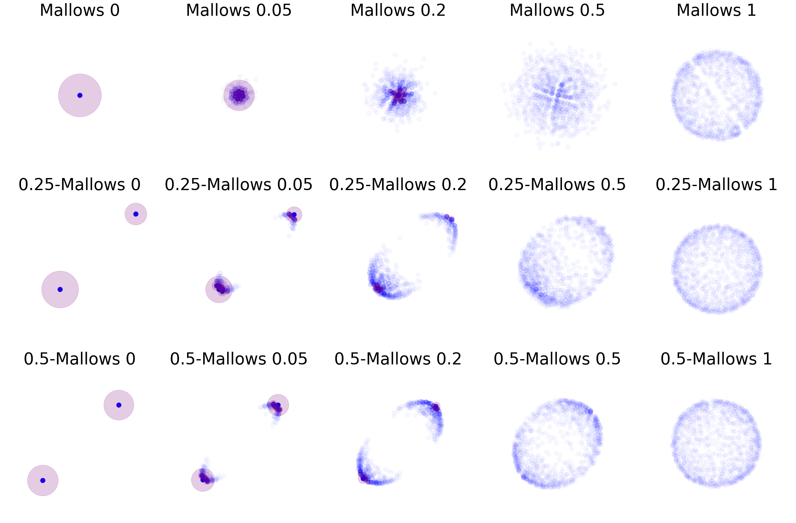
(a) Maps of Preferences (8 candidates, 1000 voters). A title “$\boldsymbol{x}$-Mallows $\boldsymbol{y}$” denotes an election from Mallows mixture model with norm-$\boldsymbol{\phi=y}$ and $\boldsymbol{\omega=x}$. We omit $\boldsymbol{x}$- when $\omega=0$.

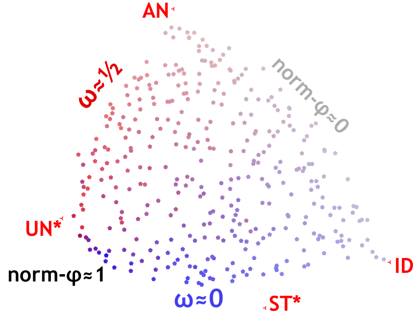
(b) A map of election in the Mallows dataset obtained using isomorphic swap distance and MDS. The color corresponds to $\omega$ parameter (blue for $\omega=0$ and red for $\omega=0.5$) and the color intensity is greater for greater ${{\mathrm{norm}\hbox{-}\phi}}$ values.

Figure 6: Mallows mixture model.

Appendix J Maps of Preferences

In this section, we present analogues of the pictures form Fig. 4 (hence, including all elections from Fig. 1), but for elections with 8 candidates and 96 voters. The method through which it is obtained is exactly the same, i.e., first we compute swap distance between every pair of votes in an election, and then we project the votes onto a 2D plane using MDS. The results are presented in Fig. 7.

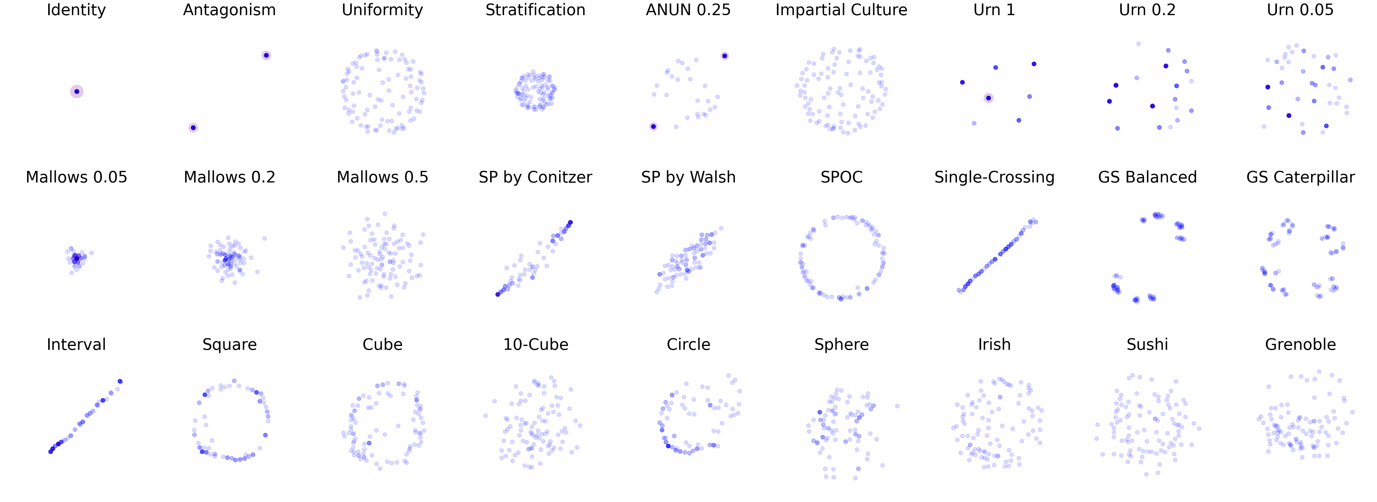
Figure 7: Maps of Preferences (8 candidates, 96 voters).

Improvement of the combined heuristic over greedy approach
Improvement of local search over greedy approach
Improvement of the combined heuristic over local search
Standard dataset	Extended dataset	Mallows dataset

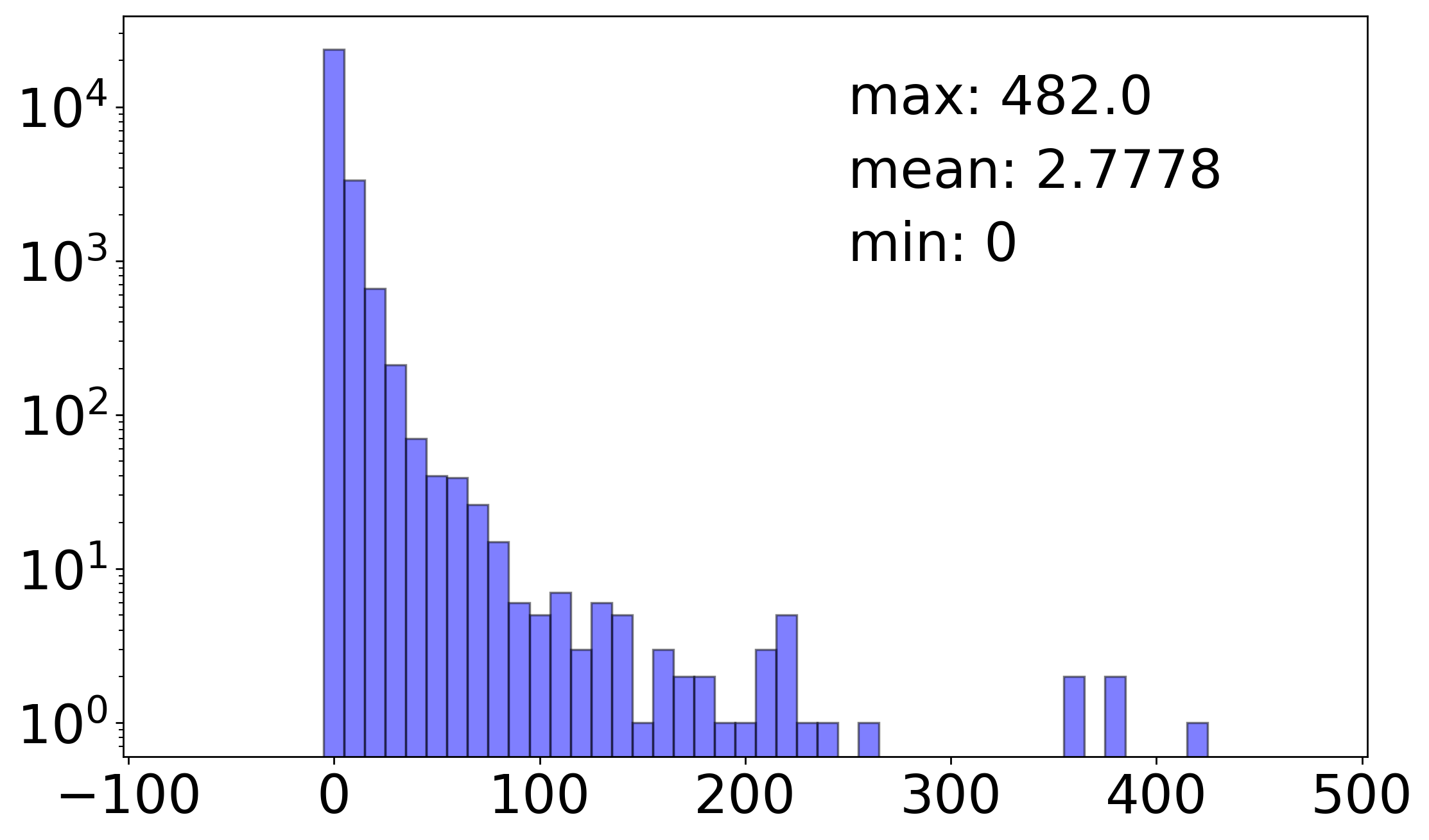
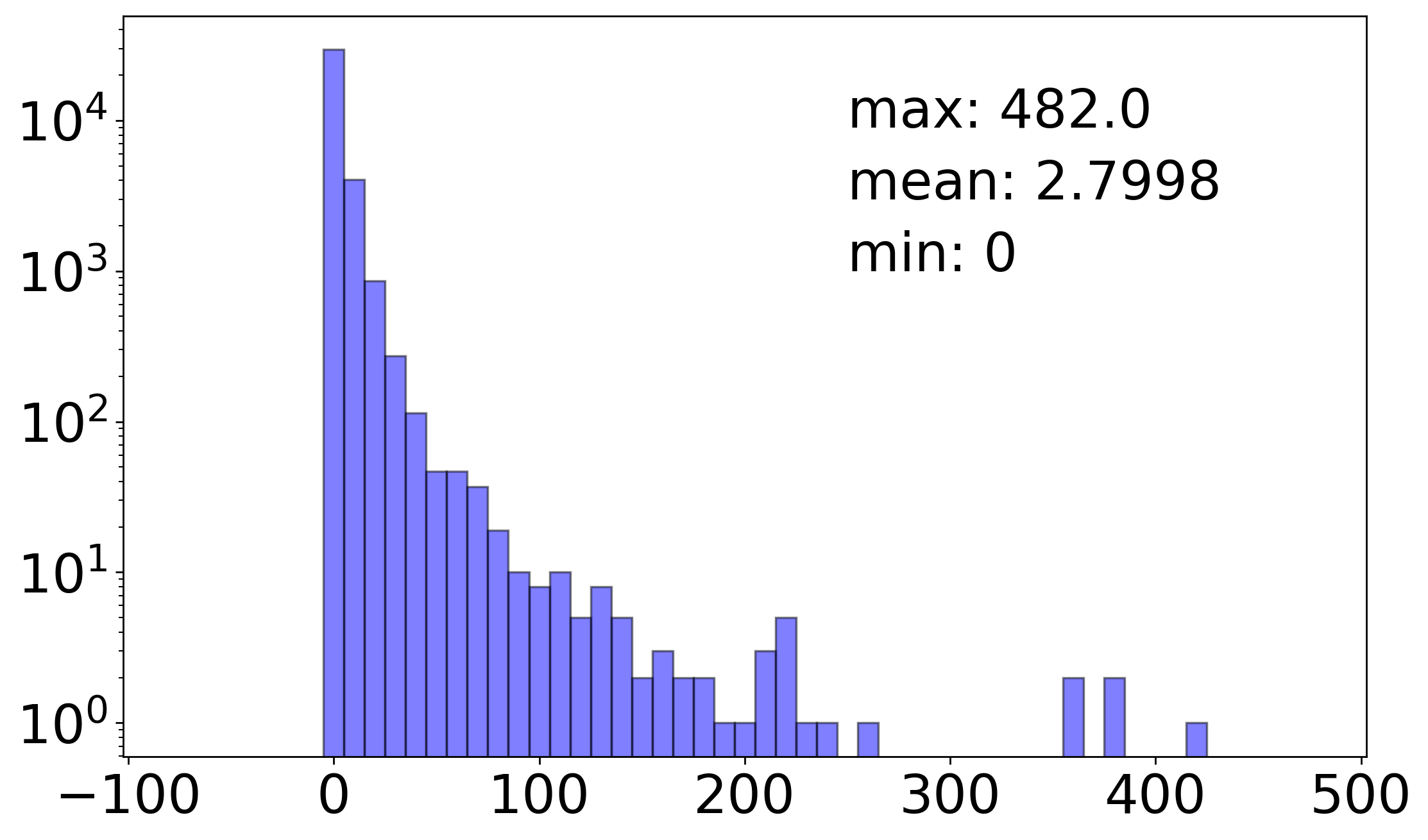
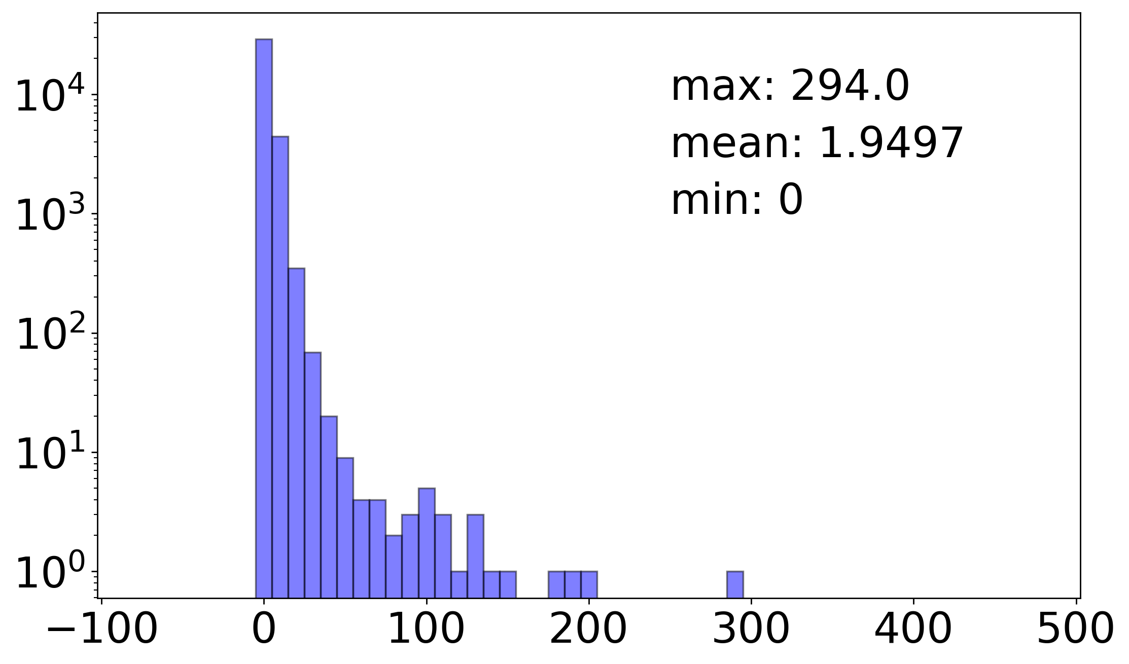
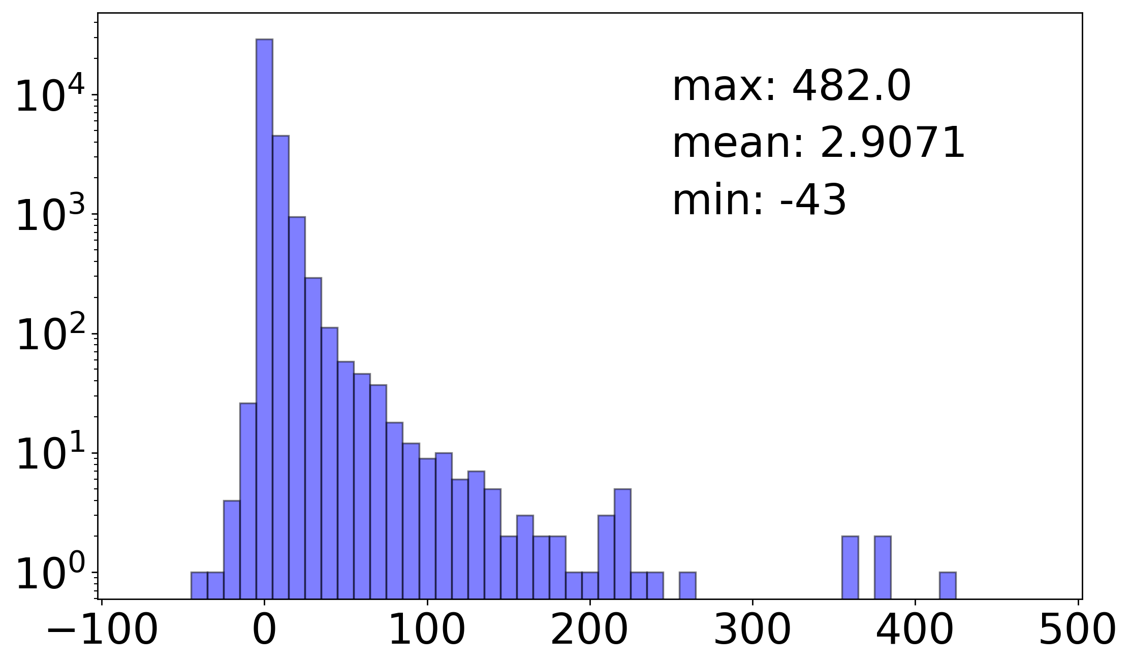
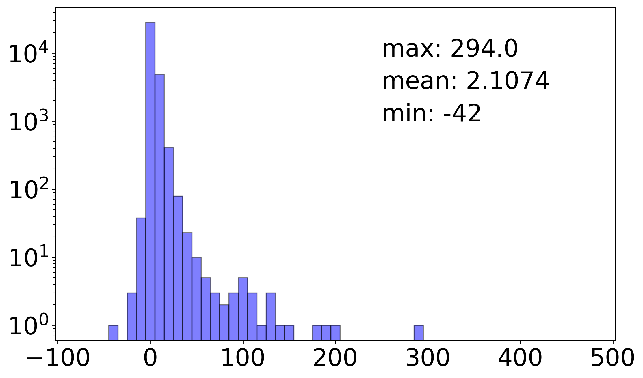
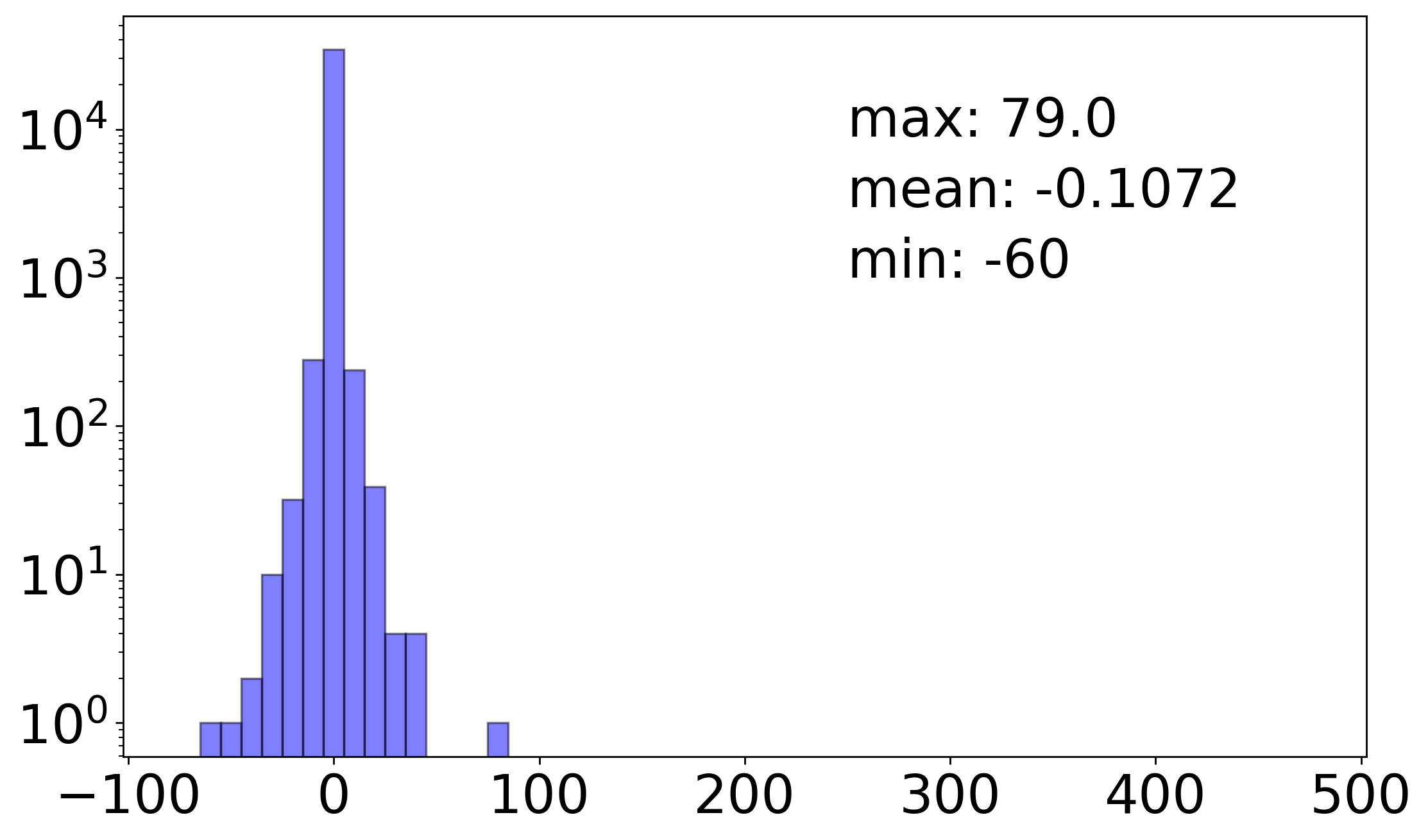
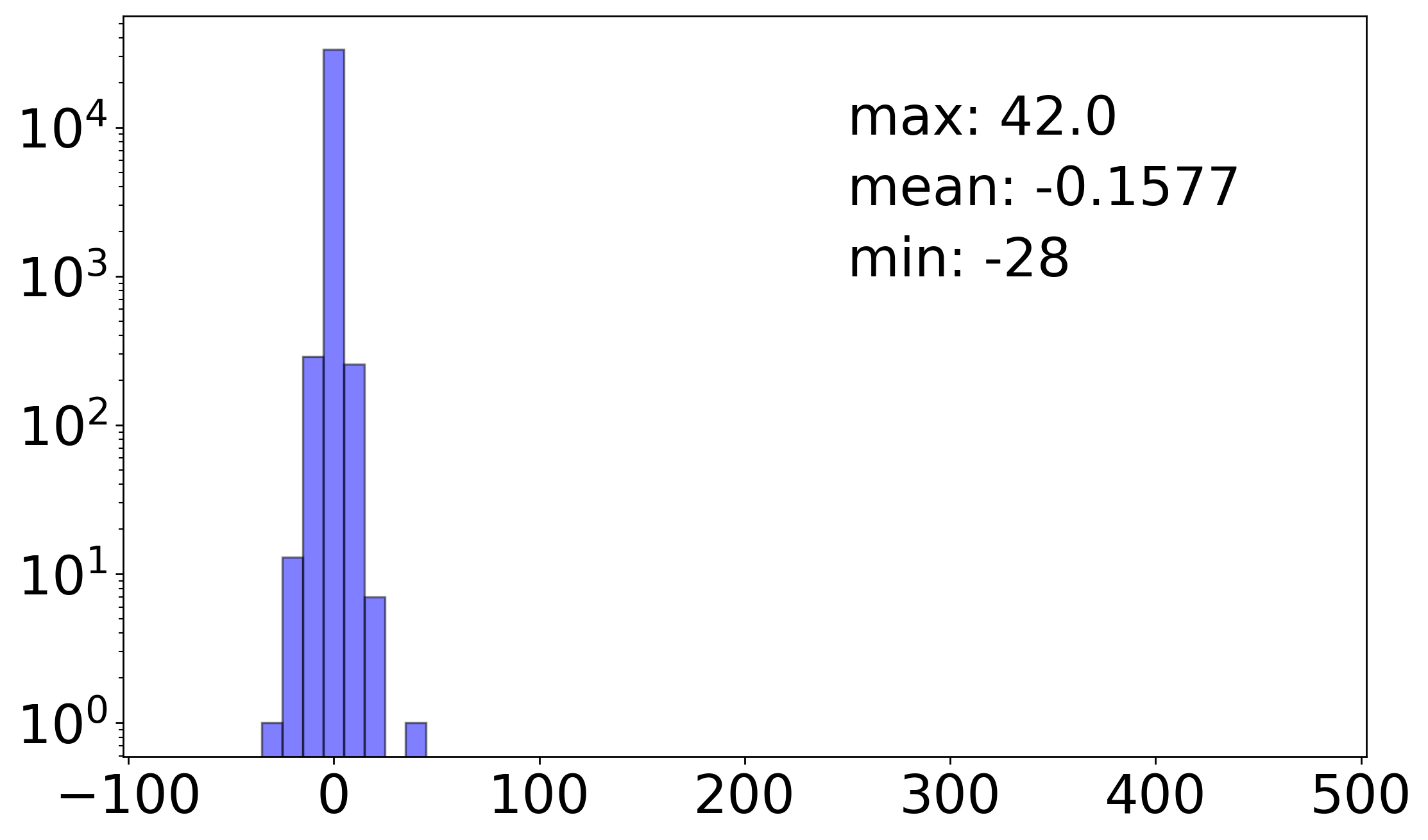
Figure 8: The histograms of differences in $k$-Kemeny distances returned by our three algorithms (note that the counts are in the logarithmic scale). The first column corresponds to the standard dataset, the second one to the extended dataset, and the third to the Mallows dataset. The maximal, average, and minimal value in each case is given.

Appendix K $\boldsymbol{k}$-Kemeny Computation Methods

In this section, we present our experiment comparing three methods of computing $k$-Kemeny distances: the greedy approach, the local search, and the combined heuristic.

For each election in all three of our datasets and every $k\in[96]$, we calculated $k$-Kemeny distance using our three methods. Then, we looked at the differences between the reported values. The histograms of differences for all three pairs of methods and all three datasets are presented in Fig. 8. We note that in the majority of cases all three methods returned exactly the same distance. However, in other cases, the differences between the reported $k$-Kemeny distance was significant, especially if we compare the combined heuristic or the local search against the greedy approach. In particular, maximal difference, 482, is observed for an election that is a mixture of AN and $\mathrm{UN}^{*}$, where voters characteristic for AN dominate by far (see Appendix F for the definition). Hence, we have two large groups of voters with exactly opposing preferences and few approximately uniformly spread votes (see Fig. 7 (5th column, 1st row) for an illustration). Then, for $k=2$, the greedy algorithm first chooses a vote that is somewhere in the middle, and then a vote that belongs to one of the two opposing groups. However, we obtain much smaller total distance, if we just set the rankings at the preference orders of the two opposing groups what both the local search and the combined heuristic managed to do.

The differences between local search and the combined heuristic are comparatively very small. On average, local search performed better than the combined heuristic, but the difference is too small to draw any conclusions. Hence, in our further calculations we simply took the better of the outcomes produced by either of these two methods.

Appendix L Plots

In this section, we present the values of all three indices for elections in our datasets. We do it in three figures (see their captions for details):

• Fig. 14 presents plots on which every election is a dot with x/y coordinates corresponding to the values of two out of three of our indices (for every pair of indices). We include also their affine transformations to show the resemblance to maps of elections from Figs. 2(a), 5, and 6(b).

• Fig. 18 shows the maps of elections in which the colors of the dots correspond to the values our indices.

• Fig. 21 depicts the correlation between the values of agreement, diversity, and polarization and the distance from ID, $\mathrm{UN}^{*}$, and AN, respectively.

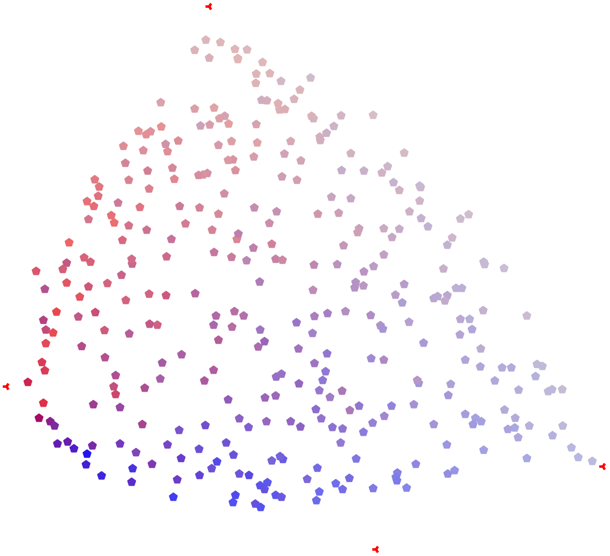
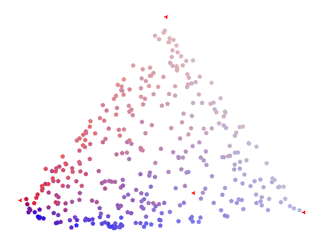
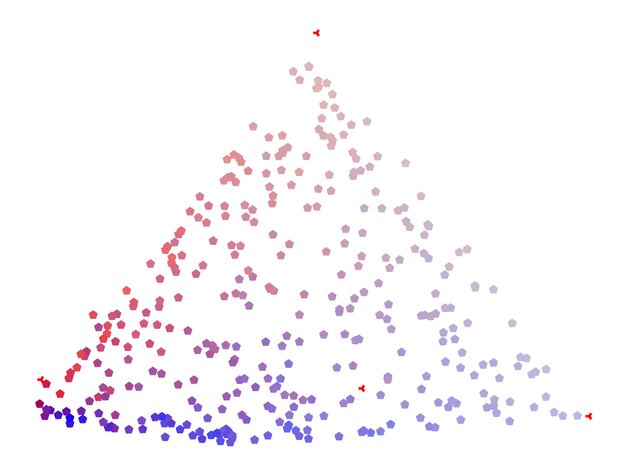
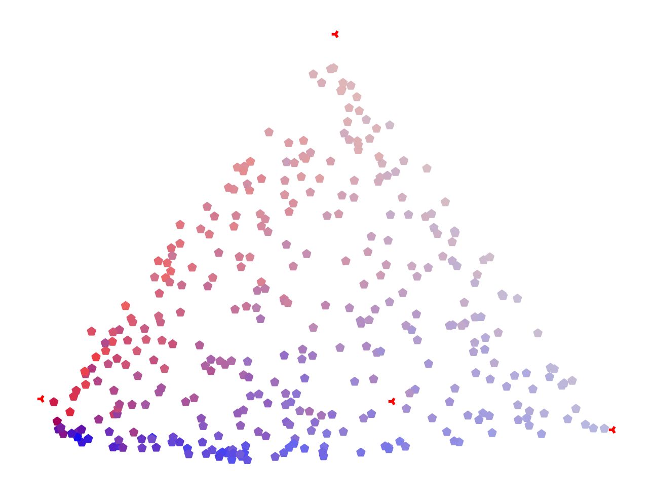
Figure 14: For each dataset, the first row presents the plots where the position of each dot corresponds to the value of our indices for elections in the dataset. In the second row, under each plot, we present its affine transformation obtained in a following way: First, we rotate the map in such a way that ID and AN form a horizontal line (with ID on the left hand side). If $\mathrm{UN}^{*}$ is below this line, we take a symmetric reflection with respect to ID–AN line. Next, we take the dot furthest from ID–AN line, $x$, and scale the height of the image, so that the distance from $x$ to ID–AN line is approximately 0.87 times the distance from ID to AN (the height of the equilateral triangle). Then, we make a shear mapping to make sure that $x$ is in equal distance to ID and AN (i.e., we move $x$ to the right or to the left, so it is in the middle, and every other dot we move in the same direction, but less, proportionally to its distance to ID–AN line). Finally, we rotate the picture by 120 degrees so that $x$ and ID form a horizontal line. For comparison, in the first column we present corresponding maps of elections from Figs. 2(a), 5, and 6(b).

Figure 18: The maps of elections from Figs. 2(a), 5, and 6(b), where the colors of the dots denote the values of our indices. The rows correspond to the datasets, and the columns correspond to the indices. The fourth one shows the sum of the indices, and the fifth one a superimposition of the first three.

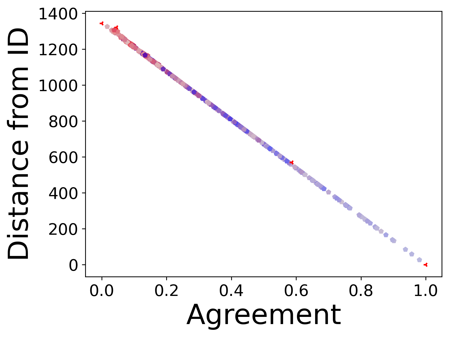
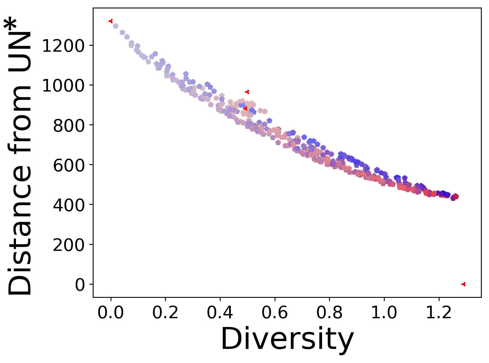
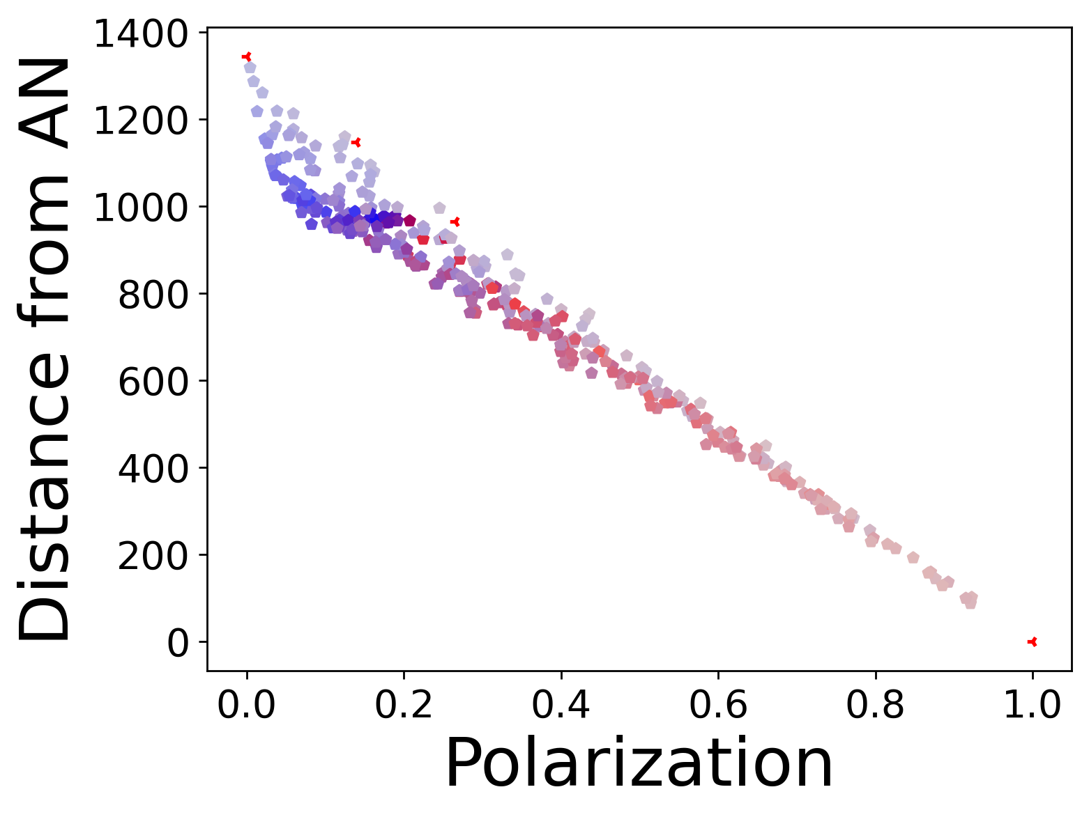
Figure 21: The plots showing the correlations between agreement, diversity, and polarization indices and distances from ID, $\mathrm{UN}^{*}$, and AN, respectively. The rows correspond to the datasets and columns to index–distance-from-election pairs.

References

- Alcalde-Unzu and Vorsatz [2013] J. Alcalde-Unzu and M. Vorsatz. Measuring the cohesiveness of preferences: An axiomatic analysis. Social Choice and Welfare, 41(4):965–988, 2013.
- Alcalde-Unzu and Vorsatz [2016] J. Alcalde-Unzu and M. Vorsatz. Do we agree? Measuring the cohesiveness of preferences. Theory and Decision, 80(2):313–339, 2016.
- Alcantud et al. [2013] J. C. R. Alcantud, R. de Andrés Calle, and J. M. Cascón. A unifying model to measure consensus solutions in a society. Mathematical and Computer Modelling, 57(7-8):1876–1883, 2013.
- Arrighi et al. [2021] E. Arrighi, H. Fernau, D. Lokshtanov, M. de Oliveira Oliveira, and P. Wolf. Diversity in Kemeny rank aggregation: A parameterized approach. In Proceedings of IJCAI-2021, pages 10–16, 2021.
- Arya et al. [2001] V. Arya, N. Garg, R. Khandekar, A. Meyerson, K. Munagala, and V. Pandit. Local search heuristic for -median and facility location problems. In Proceedings of STOC-2001, pages 21–29, 2001.
- Bartholdi et al. [1989] J. Bartholdi, III, C. Tovey, and M. Trick. Voting schemes for which it can be difficult to tell who won the election. Social Choice and Welfare, 6(2):157–165, 1989.
- Berg [1985] S. Berg. Paradox of voting under an urn model: The effect of homogeneity. Public Choice, 47(2):377–387, 1985.
- Black [1958] D. Black. The Theory of Committees and Elections. Cambridge University Press, 1958.
- Boehmer et al. [2021] N. Boehmer, R. Bredereck, P. Faliszewski, R. Niedermeier, and S. Szufa. Putting a compass on the map of elections. In Proceedings of IJCAI-2021, pages 59–65, 2021.
- Boehmer et al. [2022] N. Boehmer, P. Faliszewski, R. Niedermeier, S. Szufa, and T. Wąs. Understanding distance measures among elections. In Proceedings of IJCAI-2022, pages 102–108, 2022.
- Boehmer et al. [2023] N. Boehmer, J.-Y. Cai, P. Faliszewski, A. Z. Fan, Ł. Janeczko, A. Kaczmarczyk, and T. Wąs. Properties of position matrices and their elections. In Proceedings of IJCAI-2023, 2023. To appear.
- Bonnet et al. [2016] É. Bonnet, V. Th. Paschos, and F. Sikora. Parameterized exact and approximation algorithms for maximum k-set cover and related satisfiability problems. RAIRO Theor. Informatics Appl., 50(3):227–240, 2016.
- Bosch [2006] R. Bosch. Characterizations on Voting Rules and Consensus Measures. PhD thesis, Tilburg University, 2006.
- Byrka et al. [2017] J. Byrka, T. W. Pensyl, B. Rybicki, A. Srinivasan, and K. Trinh. An improved approximation for -median and positive correlation in budgeted optimization. ACM Transactions on Algorithms, 13(2):23:1–23:31, 2017.
- Can et al. [2015] B. Can, A. I. Ozkes, and T. Storcken. Measuring polarization in preferences. Mathematical Social Sciences, 78:76–79, 2015.
- Can et al. [2017] B. Can, A. Ozkes, and T. Storcken. Generalized measures of polarization in preferences. Technical report, HAL, 2017.
- Chamberlin and Courant [1983] B. Chamberlin and P. Courant. Representative deliberations and representative decisions: Proportional representation and the Borda rule. American Political Science Review, 77(3):718–733, 1983.
- Cohen-Addad et al. [2022] V. Cohen-Addad, A. Gupta, L. Hu, H. Oh, and D. Saulpic. An improved local search algorithm for -median. In Proceedings of SODA-2022, pages 1556–1612, 2022.
- Cohen-Addad et al. [2023] V. Cohen-Addad, F. Grandoni, E. Lee, and C. Schwiegelshohn. Breaching the 2 LMP approximation barrier for facility location with applications to -median. In Proceedings of SODA-2023, pages 940–986, 2023.
- Conitzer [2009] V. Conitzer. Eliciting single-peaked preferences using comparison queries. Journal of Artificial Intelligence Research, 35:161–191, 2009.
- Cygan et al. [2015] M. Cygan, F. V. Fomin, Ł. Kowalik, D. Lokshtanov, D. Marx, M. Pilipczuk, M. Pilipczuk, and S. Saurabh. Parameterized Algorithms. Springer, 2015.
- Dwork et al. [2001] C. Dwork, R. Kumar, M. Naor, and D. Sivakumar. Rank aggregation methods for the Web. In Proceedings of WWW-2001, pages 613–622, 2001.
- Dynes and Tierney [1994] R. Dynes and K. Tierney, editors. Disasters, Collective Behavior, and Social Organization. University of Delaware Press, 1994.
- Elkind et al. [2012] E. Elkind, P. Faliszewski, and A. Slinko. Clone structures in voters’ preferences. In Proceedings of EC-2012, pages 496–513, 2012.
- Endriss and Grandi [2014] U. Endriss and U. Grandi. Binary aggregation by selection of the most representative voters. In Proceedings of AAAI-2014, pages 668–674, 2014.
- Erdélyi et al. [2015] G. Erdélyi, M. Fellows, J. Rothe, and L. Schend. Control complexity in Bucklin and fallback voting: An experimental analysis. Journal of Computer and System Sciences, 81(4):661–670, 2015.
- Esteban and Ray [1994] J.-M. Esteban and D. Ray. On the measurement of polarization. Econometrica, 62(4):819–851, 1994.
- Faliszewski et al. [2017] P. Faliszewski, P. Skowron, A. Slinko, and N. Talmon. Multiwinner voting: A new challenge for social choice theory. In U. Endriss, editor, Trends in Computational Social Choice. AI Access Foundation, 2017.
- Faliszewski et al. [2019] P. Faliszewski, P. Skowron, A. Slinko, S. Szufa, and N. Talmon. How similar are two elections? In Proceedings of AAAI-2019, pages 1909–1916, 2019.
- Faliszewski et al. [2023] P. Faliszewski, A. Kaczmarczyk, K. Sornat, S. Szufa, and T. Wąs. Diversity, agreement, and polarization in elections. In Proceedings of IJCAI-2023, 2023. To appear.
- Gowda et al. [2023] K. N. Gowda, T. W. Pensyl, A. Srinivasan, and K. Trinh. Improved bi-point rounding algorithms and a golden barrier for -median. In Proceedings of SODA-2023, pages 987–1011, 2023.
- Hashemi and Endriss [2014] V. Hashemi and U. Endriss. Measuring diversity of preferences in a group. In Proceedings of ECAI-2014, pages 423–428, 2014.
- Hemaspaandra et al. [2005] E. Hemaspaandra, H. Spakowski, and J. Vogel. The complexity of Kemeny elections. Theoretical Computer Science, 349(3):382–391, 2005.
- Huremović and Ozkes [2022] K. Huremović and A. I. Ozkes. Polarization in networks: Identification–alienation framework. Journal of Mathematical Economics, 102:102732, 2022.
- Inada [1964] K. Inada. A note on the simple majority decision rule. Econometrica, 32(32):525–531, 1964.
- Inada [1969] K. Inada. The simple majority decision rule. Econometrica, 37(3):490–506, 1969.
- Karpov [2017] A. Karpov. Preference diversity orderings. Group Decision and Negotiation, 26(4):753–774, 2017.
- Karpov [2019] A. Karpov. On the number of group-separable preference profiles. Group Decision and Negotiation, 28(3):501–517, 2019.
- Keller et al. [2019] O. Keller, A. Hassidim, and N. Hazon. New approximations for coalitional manipulation in scoring rules. Journal of Artificial Intelligence Research, 64:109–145, 2019.
- Kemeny [1959] J. Kemeny. Mathematics without numbers. Daedalus, 88:577–591, 1959.
- Kenyon-Mathieu and Schudy [2007] C. Kenyon-Mathieu and W. Schudy. How to rank with few errors. In Proceedings of STOC-2007, pages 95–103, 2007.
- Levin et al. [2021] S. A. Levin, H. V. Milner, and C. Perrings. The dynamics of political polarization. Proceedings of the National Academy of Sciences, 118(50):e2116950118, 2021.
- Mattei and Walsh [2013] N. Mattei and T. Walsh. Preflib: A library for preferences. In Proceedings of ADT-2013, pages 259–270, 2013.
- McCabe-Dansted and Slinko [2006] J. McCabe-Dansted and A. Slinko. Exploratory analysis of similarities between social choice rules. Group Decision and Negotiation, 15:77–107, 2006.
- Mirrlees [1971] J. Mirrlees. An exploration in the theory of optimal income taxation. Review of Economic Studies, 38:175–208, 1971.
- Musco et al. [2018] C. Musco, C. Musco, and C. E. Tsourakakis. Minimizing polarization and disagreement in social networks. In Proceedings of WWW-2018, pages 369–378, 2018.
- Peters and Lackner [2020] D. Peters and M. Lackner. Preferences single-peaked on a circle. Journal of Artificial Intelligence Research, 68:463–502, 2020.
- Procaccia et al. [2008] A. D. Procaccia, J. S. Rosenschein, and A. Zohar. On the complexity of achieving proportional representation. Social Choice and Welfare, 30(3):353–362, 2008.
- Roberts [1977] K. Roberts. Voting over income tax schedules. Journal of Public Economics, 8(3):329–340, 1977.
- Skowron et al. [2015] P. Skowron, P. Faliszewski, and A. Slinko. Achieving fully proportional representation: Approximability result. Artificial Intelligence, 222:67–103, 2015.
- Sornat et al. [2022] K. Sornat, V. Vassilevska Williams, and Y. Xu. Near-tight algorithms for the Chamberlin-Courant and Thiele voting rules. In Proceedings of IJCAI-2022, pages 482–488, 2022.
- Szufa et al. [2020] S. Szufa, P. Faliszewski, P. Skowron, A. Slinko, and N. Talmon. Drawing a map of elections in the space of statistical cultures. In Proceedings of AAMAS-2020, pages 1341–1349, 2020.
- Tu and Neumann [2022] S. Tu and S. Neumann. A viral marketing-based model for opinion dynamics in online social networks. In Proceedings of WWW-2022, pages 1570–1578, 2022.
- Walsh [2011] T. Walsh. Where are the hard manipulation problems. Journal of Artificial Intelligence Research, 42(1):1–29, 2011.
- Walsh [2015] T. Walsh. Generating single peaked votes. Technical Report arXiv:1503.02766 [cs.GT], arXiv.org, March 2015.
- Williamson and Shmoys [2011] D. P. Williamson and D. B. Shmoys. The Design of Approximation Algorithms. Cambridge University Press, 2011.
- Zhu and Zhang [2022] L. Zhu and Z. Zhang. A nearly-linear time algorithm for minimizing risk of conflict in social networks. In Proceedings of KDD-2022, pages 2648–2656, 2022.