A Scalable Walsh-Hadamard Regularizer to Overcome the
Low-degree Spectral Bias of Neural Networks

Abstract

Despite the capacity of neural nets to learn arbitrary functions, models trained through gradient descent often exhibit a bias towards “simpler” functions. Various notions of simplicity have been introduced to characterize this behavior. Here, we focus on the case of neural networks with discrete (zero-one), high-dimensional, inputs through the lens of their Fourier (Walsh-Hadamard) transforms, where the notion of simplicity can be captured through the degree of the Fourier coefficients. We empirically show that neural networks have a tendency to learn lower-degree frequencies. We show how this spectral bias towards low-degree frequencies can in fact hurt the neural network’s generalization on real-world datasets. To remedy this we propose a new scalable functional regularization scheme that aids the neural network to learn higher degree frequencies. Our regularizer also helps avoid erroneous identification of low-degree frequencies, which further improves generalization. We extensively evaluate our regularizer on synthetic datasets to gain insights into its behavior. Finally, we show significantly improved generalization on four different datasets compared to standard neural networks and other relevant baselines.

1 Introduction

Classical work on neural networks shows that deep fully connected neural networks have the capacity to approximate arbitrary functions [Hornik et al., 1989, Cybenko, 1989]. However, in practice, neural networks trained through (stochastic) gradient descent have a “simplicity” bias. This notion of simplicity is not agreed upon and works such as [Arpit et al., 2017, Nakkiran et al., 2019, Valle-Perez et al., 2019, Kalimeris et al., 2019] each introduce a different notion of “simplicity”. The simplicity bias can also be studied by considering the function the neural net represents (function space view) and modeling it as Gaussian processes (GP)[Rasmussen, 2004]. Daniely et al. [2016], Lee et al. [2018] show that a wide, randomly initialized, neural network in function space is a sample from a GP with a kernel called the “Conjugate Kernel” [Daniely, 2017]. Moreover, the evolution of gradient descent on a randomly initialized neural network can be described through the “Neural Tangent Kernel” Jacot et al. [2018], Lee et al. [2019]. These works open up the road for analyzing the simplicity bias of neural nets in terms of a spectral bias in Fourier space. Rahaman et al. [2019] show empirically that neural networks tend to learn sinusoids of lower frequencies earlier on in the training phase compared to those of higher frequencies. Through the GP perspective introduced by Jacot et al. [2018], Lee et al. [2019], among others, Ronen et al. [2019], Basri et al. [2020] were able to prove these empirical findings. These results focus on continuous domains and mainly emphasize the case where the input and output are both one-dimensional.

Here, we focus on discrete domains where the input is a high-dimensional zero-one vector and we analyze the function learned by the neural network in terms of the amount of interactions among its input features in a quantitative manner. Our work is complementary to the majority of the aforementioned work that has been done on the spectral bias of neural networks in the setting of continuous, one-dimensional inputs [Ronen et al., 2019, Basri et al., 2020, Rahaman et al., 2019]. Yang and Salman [2020], Valle-Perez et al. [2019] are the first to provide spectral bias results for the discrete, higher dimensional, setting (our setting). By viewing a fully connected neural network as a function that maps zero-one vectors to real values, one can expand this function in terms of the Fourier –a.k.a Walsh-Hadamard – basis functions. The Walsh-Hadamard basis functions have a natural ordering in terms of their complexity called their degree. The degree specifies how many features each basis function is dependent upon. For example, the zero-degree basis function is the constant function and the degree-one basis functions are functions that depend on exactly one feature. Through analysis of the NTK gram matrix on the Boolean cube, Yang and Salman [2020] theoretically show that, roughly speaking, neural networks learn the lower degree basis functions earlier in training.

This tendency to prioritize simpler functions in neural networks has been suggested as a cardinal reason for their remarkable generalization ability despite their over-parameterized nature [Neyshabur et al., 2017, Arpit et al., 2017, Kalimeris et al., 2019, Poggio et al., 2018]. However, much less attention has been given to the case where the simplicity bias can hurt generalization [Tancik et al., 2020, Shah et al., 2020]. Tancik et al. [2020] show how transforming the features with random Fourier features embedding helps the neural network overcome its spectral bias and achieve better performance in a variety of tasks. They were able to explain, in a unified way, many empirical findings in computer vision research such as sinusoidal positional embeddings through the lens of overcoming the spectral bias. In the same spirit as these works, we show that the spectral bias towards low-degree functions can hurt generalization and how to remedy this through our proposed regularizer.

In more recent lines of work, regularization schemes have been proposed to directly impose priors on the function the neural network represents [Benjamin et al., 2019, Sun et al., 2019, Wang et al., 2019]. This is in contrast to other methods such as dropout, batch normalization, or other methods that regularize the weight space. In this work, we also regularize neural networks in function space by imposing sparsity constraints on their Walsh-Hadamard transform. Closest to ours is the work of Aghazadeh et al. [2021]. Inspired by studies showing that biological landscapes are sparse and contain high-degree frequencies [Sailer and Harms, 2017, Yang et al., 2019, Brookes et al., 2022, Ballal et al., 2020, Poelwijk et al., 2019], they propose a functional regularizer to enforce sparsity in the Fourier domain and report improvements in generalization scores.

Our contributions:

• We analyze the spectral behavior of a simple MLP during training through extensive experiments. We show that the standard (unregularized) network not only is unable to learn (more complex) high-degree frequencies but it also starts learning erroneous low-degree frequencies and hence overfitting on this part of the spectrum.

• We propose a novel regularizer – HashWH (Hashed Walsh Hadamard) – to remedy the aforementioned phenomenon. The regularizer acts as a “sparsifier” on the Fourier (Walsh-Hadamard) basis. In the most extreme cases, it reduces to simply imposing an $L_{1}$-norm on the Fourier transform of the neural network. Since computing the exact Fourier transform of the neural net is intractable, our regularizer hashes the Fourier coefficients to buckets and imposes an L1 norm on the buckets. By controlling the number of hash buckets, it offers a smooth trade-off between computational complexity and the quality of regularization.

• We empirically show that HashWH aids the neural network in avoiding erroneous low-degree frequencies and also learning relevant high-degree frequencies. The regularizer guides the training procedure to allocate more energy to the high-frequency part of the spectrum when needed and allocate less energy to the lower frequencies when they are not present in the dataset.

• We show on real-world datasets that, contrary to popular belief of simplicity biases for neural networks, fitting a low degree function does not imply better generalization. Rather, what is more important, is keeping the higher amplitude coefficients regardless of their degree. We use our regularizer on four real-world datasets and provide state of the art results in terms of $R^{2}$ score compared to standard neural networks and other baseline ML models, especially for the low-data regime.

2 Background

In this section, we first review Walsh Hadamard transforms, and notions of degree and sparsity in the Fourier (Walsh-Hadamard) domain [O’Donnell, 2014]. Next, we review the notion of simplicity biases in neural networks and discuss why they are spectrally biased toward low-degree functions.

2.1 Walsh Hadamard transforms

Let $g:\{0,1\}^{n}\rightarrow\operatorname{\mathbb{R}}$ be a function mapping Boolean zero-one vectors to the real numbers, also known as a “pseudo-boolean” function. The family of $2^{n}$ functions $\{\Psi_{f}:\{0,1\}^{n}\rightarrow\operatorname{\mathbb{R}}|f\in\{0,1\}^{n}\}$ defined below consists of the Fourier basis functions. This family forms a basis over the vector space of all pseudo-boolean functions:

$$\Psi_{f}(x)=\frac{1}{\sqrt{2^{n}}}(-1)^{\langle f,x\rangle},f,x\in\{0,1\}^{n}$$

where ${\langle f,x\rangle}=\sum_{i}f_{i}x_{i}$. Here, $f\in\{0,1\}^{n}$ is called the frequency of the basis function. For any frequency $f\in\{0,1\}^{n}$ we denote its degree by $\text{deg}(f)$ which is defined as the number of non-zero elements. For example, $f_{1}=[0,0,0,0,0]$ and $f_{2}=[0,0,1,0,1]$ have degrees $\text{deg}(f_{1})=0$ and $\text{deg}(f_{2})=2$, respectively. One can think of the degree as a measure of the complexity of basis functions. For example, $\Psi_{0}(x)$ is constant, and $\Psi_{e_{i}}(x)$ where $e_{i}$ is a standard basis vector ($\text{deg}(e_{i})=1$) only depends on feature $i$ of the input. It is equal to $+1$ when feature $i$ is zero and equal to $-1$ when feature $i$ is one. More generally, a degree $d$ basis function depends on exactly $d$ input features.

Since the Fourier basis functions form a basis for the vector space of all pseudo-boolean functions, any function $g:\{0,1\}^{n}\rightarrow\operatorname{\mathbb{R}}$ can be written as a unique linear combination of these basis functions:

$$g(x)=\frac{1}{\sqrt{2^{n}}}\sum\limits_{f\in\{0,1\}^{n}}\widehat{g}(f)(-1)^{\langle f,x\rangle}$$

The (unique) coefficients $\widehat{g}(f)$ are called the “Fourier coefficients” or “Fourier amplitudes” and are computed as $\widehat{g}(f)=\frac{1}{\sqrt{2^{n}}}\sum\limits_{x\in\{0,1\}^{n}}g(x)(-1)^{\langle f,x\rangle}$. The Fourier spectrum of $g$ is the vector consisting of all of its $2^{n}$ Fourier coefficients, which we denote by the bold symbol $\widehat{\mathbf{g}}\in\mathbb{R}^{2^{n}}$. Assume $\mathbf{X}\in\{0,1\}^{2^{n}\times n}$ to be the matrix of an enumeration over all possible $n$-dimensional binary sequences ($\{0,1\}^{n}$), and $\mathbf{g}(\mathbf{X})\in\mathbb{R}^{2^{n}}$ to be the vector of $g$ evaluated on the rows of $\mathbf{X}$. We can compute the Fourier spectrum using Walsh-Hadamard transform as $\widehat{\mathbf{g}}=\frac{1}{\sqrt{2^{n}}}\mathbf{H}_{n}\mathbf{g}(\mathbf{X})$, where $\mathbf{H}_{n}\in\{\pm 1\}^{2^{n}\times 2^{n}}$ is the orthogonal Hadamard matrix (see Appendix A).

Lastly, we define the support of $g$ as the set of frequencies with non-zero Fourier amplitudes $\text{supp}(g):=\{f\in\{0,1\}^{n}|\widehat{g}(f)\neq 0\}$. The function $g$ is called $k$-sparse if $|\text{supp}(g)|\leq k$. The function $g$ is called of degree $d$ if all frequencies in its support have degree at most $d$.

2.2 Spectral bias theory

The function that a ReLU neural network represents at initialization can be seen as a sample from a GP $N(0,K)$ in the infinite width limit [Daniely et al., 2016, Lee et al., 2018] (randomness is over the initialization of the weights and biases). The kernel $K$ of the GP is called the “Conjugate Kernel” [Daniely et al., 2016] or the “nn-GP kernel” [Lee et al., 2018]. Let the kernel Gram matrix $\mathcal{K}$ be formed by evaluating the kernel on the Boolean cube i.e. $\{0,1\}^{n}$ and let $\mathcal{K}$ have the following spectral decomposition: $\mathcal{K}=\sum\limits_{i=1}^{2^{n}}\lambda_{i}u_{i}u_{i}^{\top}$, where we assume that the eigenvalues $\lambda_{1}\geq\dots\geq\lambda_{2^{n}}$ are in decreasing order. Each sample of the GP can be obtained as $\sum\limits_{i=1}^{2^{n}}\lambda_{i}\bm{w_{i}}u_{i},\bm{w_{i}}\sim\mathcal{N}(0,1)$. Say that $\lambda_{1}\gg\sum_{i\geq 2}\lambda_{i}$. Then a sample from the GP will, roughly speaking, look very much like $u_{1}$.

Let $u_{f},f\in\{0,1\}^{n}$ be obtained by evaluating the Fourier basis function $\Psi_{f}$ at the $2^{n}$ possible inputs on $\{0,1\}^{n}$. Yang and Salman [2020] show that $u_{f}$ is a eigenvector for $\mathcal{K}$. Moreover, they show (weak) spectral bias results in terms of the degree of $f$. Namely, the eigenvalues corresponding to higher degrees have smaller values . The result is weak as they do not provide a rate as to which the eigenvalues decrease with increasing degrees. Their results show that neural networks are similar to low-degree functions at initialization.

Other works show that in infinite-width neural networks weights after training via (stochastic) gradient descent do not end up too far from the initialization [Chizat et al., 2019, Jacot et al., 2018, Du et al., 2019, Allen-Zhu et al., 2019a, b], referred to as “lazy training” by Chizat et al. [2019]. Lee et al. [2018, 2019] show that training the last layer of a randomly initialized neural network via full batch gradient descent for an infinite amount of time corresponds to GP posterior inference with the kernel $K$. Jacot et al. [2018], Lee et al. [2019] proved that when training all the layers of a neural network (not just the final layer), the evolution can be described by a kernel called the “Neural Tangent Kernel” and the trained network yields the mean prediction of GP $N(0,K_{NTK})$ [Yang and Salman, 2020] after an infinite amount of time. Yang and Salman [2020] again show that $u_{f}$ are eigenvectors and weak spectral bias holds. Furthermore, Yang and Salman [2020] provides empirical results for the generalization of neural nets of different depths on datasets arising from $k=1$-sparse functions of varying degrees.

3 Low-degree spectral bias

In this section, we conduct experiments on synthetically generated datasets to show neural networks’ spectral bias and their preference toward learning lower-degree functions over higher-degree ones. Firstly, we show that the neural network is not able to pick up the high-degree frequency components. Secondly, it can learn erroneous lower-degree frequency components. To address these issues, in Section 4, we introduce our regularization scheme called HashWH (Hashed Walsh Hadamard) and demonstrate how it can remedy both problems.

3.1 Fourier spectrum evolution

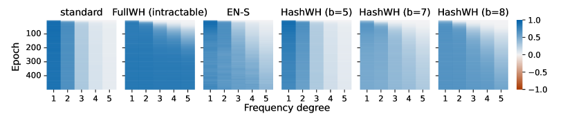
(a) Target support

(b) Whole Fourier spectrum

Figure 1: Evolution of the Fourier spectrum during training. Standard is the unregularized neural network. FullWH imposes $L_{1}$-norm regularization on the exact Fourier spectrum and is intractable. EN-S alternates between computing a sparse Fourier approximation (computationally very expensive) and regularization. HashWH (ours) imposes $L_{1}$ regularization on the hashed spectrum. Figure (a) is limited to the target support. The standard neural network is unable to learn higher degree frequencies. Our regularizer fixes this. Figure (b) is on the whole spectrum. The standard neural network picks up erroneous low-degree frequencies while not being able to learn the higher-degree frequencies. Our regularizer fixes both problems.

We analyze the evolution of the function learned by neural networks during training. We train a neural network on a dataset arising from a synthetically generated sparse function with a low-dimensional input domain. Since the input is low-dimensional it allows us to calculate the Fourier spectrum of the network (exactly) at the end of each epoch.

Setup. Let $g^{*}:\{0,1\}^{10}\rightarrow\mathbb{R}$ be a synthetic function with five frequencies in its support with degrees 1 to 5 ($\text{supp}(g^{*})=\{f_{1},f_{2},f_{3},f_{4},f_{5}\},\text{deg}(f_{i})=i$), all having equal Fourier amplitudes of $\widehat{g}^{*}(f_{i})=1$. Each $f_{i}$ is sampled uniformly at random from all possible frequencies of degree $i$. The training set is formed by drawing uniform samples from the Boolean cube $x\sim\mathcal{U}_{\{0,1\}^{10}}$ and evaluating $g^{*}(x)$.

We draw five such target functions $g^{*}$ (with random support frequencies). For each draw of the target function, we create five different datasets all with 200 training points and sampled uniformly from the input domain but with different random seeds. We then train a standard five-layer fully connected neural network using five different random seeds for the randomness in the training procedure (such as initialization weights and SGD). We aggregate the results over the $125$ experiments by averaging. We experiment the same setting with three other training set sizes. Results with training set size other than 200 and further setup details are reported in Appendices F.1 and D, respectively.

Results. We first inspect the evolution of the learned Fourier spectrum over different epochs and limited to the target support ($\text{supp}(g^{*})$). Figure 1(a) shows the learned amplitudes for frequencies in the target support at each training epoch. Aligned with the literature on simplicity bias [Valle-Perez et al., 2019, Yang and Salman, 2020], we observe that neural networks learn the low-degree frequencies earlier in the epochs. Moreover, we can see in the left-most figure in Figure 1(a) that despite eventually learning low-degree frequencies, the standard network is unable to learn high-degree frequencies.

Next, we expand the investigation to the whole Fourier spectrum instead of just focusing on the support frequencies. The first row of Figure 1(b) shows the evolution of the Fourier spectrum during training and compares it to the spectrum of the target function on the bottom row. We average the spectrum linked to one of the five target synthetic functions (over the randomness of the dataset sampling and training procedure) and report the other four in Appendix F.1. We observe that in addition to the network not being able to learn the high-degree frequencies, the standard network is prone to learning incorrect low-degree frequencies as well.

4 Overcoming the spectral bias via regularization

Now, we introduce our regularization scheme HashWH (Hashed Walsh-Hadamard). Our regularizer is essentially a “sparsifier” in the Fourier domain. That is, it guides the neural network to have a sparse Fourier spectrum. We empirically show later how sparsifying the Fourier spectrum can both stop the network from learning erroneous low-degree frequencies and aid it in learning the higher-degree ones, hence remedying the two aforementioned problems.

Assume $\mathcal{L}_{net}$ is the loss function that a standard neural network minimizes, e.g., the MSE loss in the above case. We modify it by adding a regularization term $\lambda\mathcal{L}_{sparsity}$. Hence the total loss is given by: $\mathcal{L}=\mathcal{L}_{net}+\lambda\mathcal{L}_{sparsity}$.

The most intuitive choice is $\mathcal{L}_{sparsity}=\|\widehat{\mathbf{g_{N}}}\|_{0}$, where $\widehat{\mathbf{g_{N}}}$ is the Fourier spectrum of the neural network function $g_{N}:\{0,1\}^{n}\rightarrow\operatorname{\mathbb{R}}$. Since the $L_{0}$-penalty’s derivative is zero almost everywhere, one can use its tightest convex relaxation, the $L_{1}$-norm, which is also sparsity-inducing, as a surrogate loss. Aghazadeh et al. [2021] use this idea and name it as Epistatic-Net or “EN” regularization: $\mathcal{L}_{EN}:=\mathcal{L}_{net}+\lambda\|\widehat{\mathbf{g_{N}}}\|_{1}$. In this work, we call this regularization FullWH (Full Walsh Hadamard transform).

FullWH requires the evaluation of the network output on all $2^{n}$ possible inputs at each iteration of back-prop. Therefore, the computational complexity grows exponentially with the number of dimensions $n$, making it computationally intractable for $n>20$ in all settings of practical importance.

Aghazadeh et al. [2021] also suggest a more scalable version of FullWH, called “EN-S”, which roughly speaking, alternates between computing the sparse approximate Fourier transform of the network at the end of each epoch and doing normal back-prop, as opposed to the exact computation of the exact Fourier spectrum when back-propagating the gradients. In our experiments, we show EN-S can be computationally expensive because the sparse Fourier approximation primitive can be time-consuming. For a comprehensive comparison see Appendix B.3. Later, we show that empirically, it is also less effective in overcoming the spectral bias as measured by achievable final generalization error.

4.1 HashWH

We avoid the exponentially complex burden of computing the exact Fourier spectrum of the network by employing a hashing technique to approximate the regularization term $\lambda\|\widehat{\mathbf{g_{N}}}\|_{1}$. Let $g:\{0,1\}^{n}\rightarrow\mathbb{R}$ be a pseudo-boolean function. We define the lower dimensional function $u_{\mathbf{\sigma}}:\{0,1\}^{b}\rightarrow\mathbb{R}$, where $b\ll n$, by sub-sampling $g$ on its domain: $u_{\mathbf{\sigma}}(\tilde{x})\triangleq\sqrt{\frac{2^{n}}{2^{b}}}\ g(\mathbf{\sigma}\tilde{x}),\ \tilde{x}\in\{0,1\}^{b}$ where $\mathbf{\sigma}\in\{0,1\}^{n\times b}$ is some matrix which we call the hashing matrix. The matrix-vector multiplication $\sigma\tilde{x}$is taken modulo 2. $u_{\sigma}$ is defined by sub-sampling $g$ on all the points lying on the (at most) $b$-dimensional subspace spanned by the columns of the hashing matrix $\sigma$. The special property of sub-sampling the input space from this subspace is in the arising Fourier transform of $u_{\sigma}$ which we will explain next.

The Fourier transform of $u_{\mathbf{\sigma}}$ can be derived as (see Appendix B.1):

$$\widehat{u}_{\mathbf{\sigma}}(\tilde{f})=\sum_{f\in\{0,1\}^{n}:\ \mathbf{\sigma}^{\top}f=\tilde{f}}\widehat{g}(f),\ \tilde{f}\in\{0,1\}^{b}$$ (1)

One can view $\widehat{u}_{\mathbf{\sigma}}(\tilde{f})$ as a “bucket” containing the sum of all Fourier coefficients $\widehat{g}(\tilde{f})$ that are “hashed” (mapped) into it by the linear hashing function $h(f)=\sigma^{\top}f$. There are $2^{b}$ such buckets and each bucket contains frequencies lying in the kernel (null space) of the hashing map plus some shift.

In practice, we let $\mathbf{\sigma}\sim\mathcal{U}_{\{0,1\}^{n\times b}}$ be a uniformly sampled hash matrix that is re-sampled after each iteration of back-prop. Let $\mathbf{X}_{b}\in\{0,1\}^{2^{b}\times b}$ be a matrix containing as rows the enumeration over all points on the Boolean cube $\{0,1\}^{b}$. Our regularization term approximates (4) and is given by:

$$\mathcal{L}_{\textsc{HashWH}}\triangleq\mathcal{L}_{net}+\lambda\|\mathbf{H}_{b}\mathbf{g_{N}}(\mathbf{X}_{b}\mathbf{\sigma}^{T})\|_{1}=\mathcal{L}_{net}+\lambda\|\widehat{\mathbf{u_{\mathbf{\sigma}}}}\|_{1}$$

That is, instead of imposing the $L_{1}$-norm directly on the whole spectrum, this procedure imposes the norm on the “bucketed” (or partitioned) spectrum where each bucket (partition) contains sums of coefficients mapped to it. The larger $b$ is the more partitions we have and the finer-grained the sparsity-inducing procedure is. Therefore, the quality of the approximation can be controlled by the choice of $b$. Larger $b$ allows for a finer-grained regularization but, of course, comes at a higher computational cost because a Walsh-Hadamard transform is computed for a higher dimensional sub-sampled function $u$. Note that $b=n$ corresponds to hashing to $2^{n}$ buckets. As long as the hashing matrix is invertible, this precisely is the case of FullWH regularization.

The problem with the above procedure arises when, for example, two “important” frequencies $f_{1}$ and $f_{2}$ are hashed into the same bucket, i.e., $\mathbf{\sigma}^{\top}f_{1}=\mathbf{\sigma}^{\top}f_{2}$, an event which we call a “collision”. This can be problematic when the absolute values $|\widehat{g}(f_{1})|$ and $|\widehat{g}(f_{2})|$ are large (hence they are important frequencies) but their sum can cancel out due to differing signs. In this case, the hashing procedure can zero out the sum of these coefficients. We can reduce the probability of a collision by increasing the number of buckets, i.e., increasing $b$ [Alon et al., 1999].

In Appendix B.2 we show that the expected number of collisions $C$ is given by: $\mathbb{E}[C]=\frac{(k-1)^{2}}{2^{b}}$ which decreases linearly with the number of buckets $2^{b}$. Furthermore, we can upper bound the probability $p$ that a given important frequency $f_{i}$ collides with any other of the $k-1$ important frequencies in one round of hashing. Since we are independently sampling a new hashing matrix $\mathbf{\sigma}$ at each round of back-prop, the number of collisions of a given frequency over the different rounds has a binomial distribution. In Appendix B.2 we show that picking $b\geq\log_{2}(\frac{k-1}{\epsilon}),\epsilon>0$ guarantees that collision of a given frequency happens approx. an $\epsilon$-fraction of the $T$ rounds, and not much more.

Fourier spectrum evolution of different regularization methods. We analyze the effect of regularizing the network with various Fourier sparsity regularizers in the setting of the previous section. Our regularizers of interest are FullWH, EN-S with $m=5$ ($2^{m}$ is the number of buckets their sparse Fourier approximation algorithm hashes into), and HashWH with $b\in\{5,7,8\}$.

Returning to Figure 1(a), we see that despite the inability of the standard neural network in picking up the high-degree frequencies, all sparsity-inducing regularization methods display the capacity for learning them. FullWH is capable of perfectly learning the entire target support. It can also be seen that increasing the size of the hashing matrix in HashWH (ours) boosts the learning of high-degree frequencies. Furthermore, Figure 1(b) shows that in addition to the better performance of the sparsity-inducing methods in learning the target support, they are also better at filtering out non-relevant low-degree frequencies.

We define a notion of approximation error which is basically the normalized energy of the error in the learned Fourier spectrum on an arbitrary subset of frequencies.

Metric 4.1 (Spectral Approximation Error (SAE)).

Let $g_{N}:\{0,1\}^{n}\rightarrow\mathbb{R}$ be an approximation of the target function $g^{*}:\{0,1\}^{n}\rightarrow\mathbb{R}$. Consider a subset of frequencies $S\subseteq\{0,1\}^{n}$, and assume $\widehat{\mathbf{g_{N}}}_{S}$ and $\widehat{\mathbf{g^{*}}}_{S}$ to be the vector of Fourier coefficients of frequencies in $S$, for $g_{N}$ and $g^{*}$ respectively. As a measure of the distance between $g_{N}$ and $g$ on the subset of frequencies $S$, we define Spectral Approximation Error as: $\text{SAE}=\frac{\|\widehat{\mathbf{g_{N}}}_{S}-\widehat{\mathbf{g^{*}}}_{S}\|^{2}_{2}}{\|\widehat{\mathbf{g^{*}}}_{S}\|^{2}_{2}}$

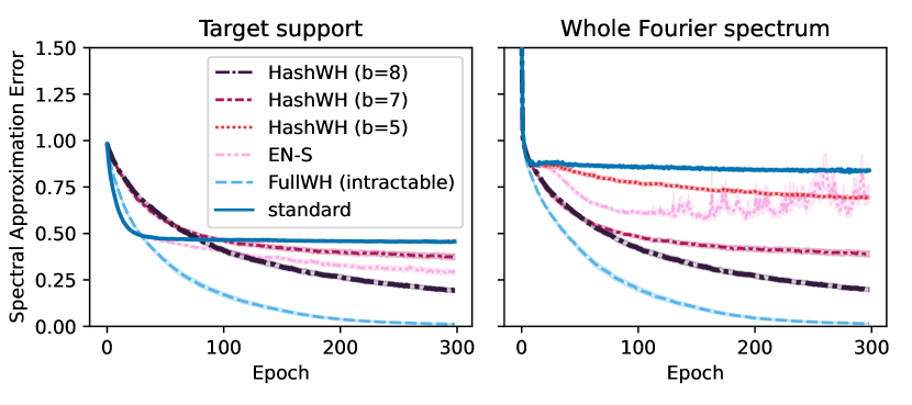
Figure 2: Evolution of the spectral approximation error during training. The left plot limits the error to the target support, while the right one considers the whole Fourier spectrum. For the standard neural network, the SAE is considerably worse on the full spectrum which shows the importance of eliminating the erroneous frequencies that are not in the support of the target function. We also see the graceful scaling of SAE of HashWH (ours) with the hashing matrix size.

Figure 2 shows the SAE of the trained network using different regularization methods over epochs, for both when $S$ is target support as well as when $S=\{0,1\}^{n}$ (whole Fourier spectrum). The standard network displays a significantly higher (worse) SAE on the whole Fourier spectrum compared to the target support, while Walsh-Hadamard regularizers exhibit consistent performance across both. This shows the importance of enforcing the neural network to have zero Fourier coefficients on the non-target frequencies. Moreover, we can see HashWH (ours) leads to a reduction in SAE that can be smoothly controlled by the size of its hashing matrix.

To gain more insight, we split the frequencies into subsets $S$ consisting of frequencies with the same degree. We visualize the evolution of SAE and also the Fourier energy of the network defined as $\|\widehat{\mathbf{g_{N}}}_{S}\|_{2}^{2}$ in Figure 3. Firstly, the energy of high-degree frequencies is essentially zero for the standard neural network when compared to the low-degree frequencies, which further substantiates the claim that standard neural network training does not learn any high-degree frequencies. We can see that our HashWH regularization scheme helps the neural network learn higher degree frequencies as there is more energy in the high degree components. Secondly, looking at the lower degrees 2 and 3 we can see that the standard neural network reduces the SAE up to some point but then starts overfitting. Looking at the energy plot one can attribute the overfitting to picking up irrelevant degree 2 and 3 frequencies. We see that the regularization scheme helps prevent the neural net from overfitting on the low-degree frequencies and their SAE reduces roughly monotonously. We observe that HashWH (ours) with a big enough hashing matrix size exhibits the best performance among tractable methods in terms of SAE on all degrees. Finally, we can see HashWH is distributing the energy to where it should be for this dataset: less in the low-degree and more in the high-degree frequencies.

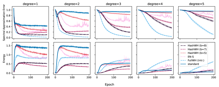
Figure 3: Evolution of the Spectral Approximation Error (SAE) and energy of the network during training, split by frequency degree. Firstly, in a standard neural network, the energy of high-degree frequencies is essentially zero compared to low-degree frequencies. Secondly, for low degrees (2 and 3) the energy continues to increase while the SAE exhibits overfitting behavior. This implies the neural network starts learning erroneous low-degree frequencies after some epochs. Our regularizer prevents overfitting in lower degrees and enforces higher energy on higher-degree frequencies. Regularized networks show lower energies for lower degrees and higher energy for higher degrees when compared to the standard neural network.

Finally, it is worth noting that our regularizer makes the neural network behave more like a decision tree. It is well known that ensembles of decision tree models have a sparse and low-degree Fourier transform [Kushilevitz and Mansour, 1991]. Namely, let $g:\{0,1\}^{n}\rightarrow\operatorname{\mathbb{R}}$ be a function that can be represented as an ensemble of $T$ trees each of depth at most $d$. Then $g$ is $k=O(T\cdot 4^{d})$-sparse and of degree at most $d$ (Appendix E.1). Importantly, their spectrum is exactly sparse and unlike standard neural networks, which seem to “fill up” the spectrum on the low-degree end, i.e., learn irrelevant low-degree coefficients, decision trees avoid this. Decision trees are well-known to be effective on discrete/tabular data [Arik and Pfister, 2021], and our regularizer prunes the spectrum of the neural network so it behaves similarly.

5 Experiments

In this section, we first evaluate our regularization method on higher dimensional input spaces (higher $n$) on synthetically generated datasets. In this setting, FullWH is not applicable due to its exponential runtime in $n$. In addition, we allow varying training set sizes to showcase the efficacy of the regularizer in improving generalization at varying levels in terms of the number of training points in the dataset and especially in the low-data sample regime. Next, we move on to four real-world datasets. We first show the efficacy of our proposed regularizer hashWH on real-world datasets in terms of achieving better generalization errors, especially in the low-data sample regimes. Finally, using an ablation study, we experimentally convey that the low-degree bias does not result in lower generalization error.

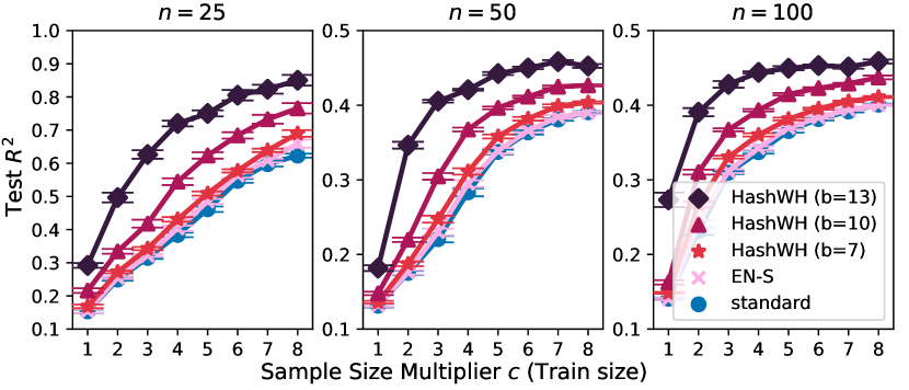
(a) Generalization comparison

(b) Runtime comparison

Figure 4: (a) Generalization performance on learning a synthetic function $g^{*}:\{0,1\}^{n}\rightarrow\mathbb{R}$ with train set size: $c\cdot 25n$ (b) Best achievable test $R^{2}$ (I) at end of each epoch (II) up to a certain time (seconds). (III) Shows the early stopped $R^{2}$ score vs. time (seconds). We provide significant improvements across all training sizes over EN-S and standard neural networks, while also showing an order of magnitude speed-up compared to EN-S.

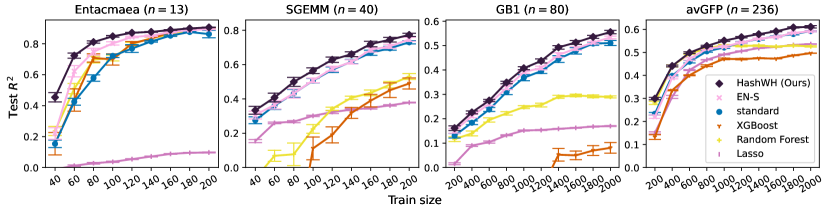
(a) Performance on learning real datasets

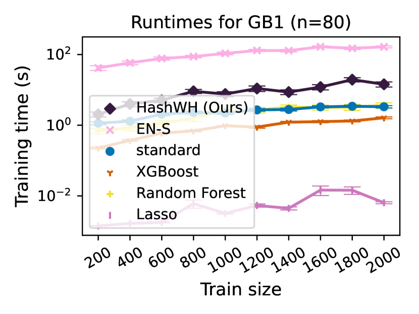
(b) Runtimes for GB1

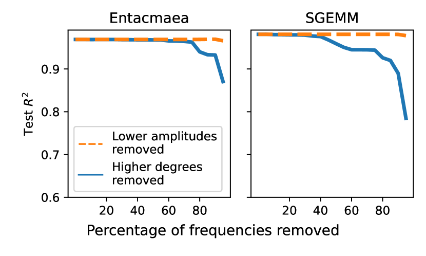
(c) Ablation studies

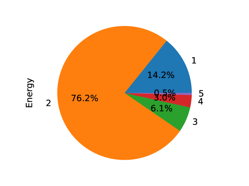
(d) Energy distribution over
degrees in Entacmaea

Figure 5: (a) Generalization performance of standard and regularized neural networks and benchmark ML models on four real datasets. (b) Training times of different models on the GB1 dataset (c) Results of an ablation study on the potential effect of simplicity bias in the generalization error. This figure shows picking higher amplitude coefficients results in better generalization compared to picking the lower degree terms (d) Distribution of the energy over degree-based sets of frequencies in Entacmaea’s top 100 Fourier coefficients. This shows high-degree components constitute a non-negligible portion of the energy of the function.

5.1 Synthetic data

Setup. Again, we consider a synthetic pseudo-boolean target function $g^{*}:\{0,1\}^{n}\rightarrow\mathbb{R}$, which has $25$ frequencies in its support $|\text{supp}(g^{*})|=25$, with the degree of maximum five, i.e., $\forall f\in\text{supp}(g^{*}):\text{deg}(f)\leq 5$. To draw a $g^{*}$, we sample each of its support frequencies $f_{i}$ by first uniformly sampling its degree $d\sim\mathcal{U}_{\{1,2,3,4,5\}}$, based on which we then sample $f_{i}\sim\{f\in\{0,1\}^{n}|\text{deg}(f)=d\}$ and its corresponding amplitude uniformly $\widehat{g^{*}}(f_{i})\sim\mathcal{U}_{[-1,1]}$.

We draw $g^{*}$ as above for different input dimensions $n\in\{25,50,100\}$. We pick points uniformly at random from the input domain $\{0,1\}^{n}$ and evaluate $g^{*}$ to generate datasets of various sizes: we generate five independently sampled datasets of size $c\cdot 25n$, for different multipliers $c\in\{1,..,8\}$ (40 datasets for each $g^{*}$). We train a 5-layer fully-connected neural network on each dataset using five different random seeds to account for the randomness in the training procedure. Therefore, for each $g^{*}$ and dataset size, we train and average over 25 models to capture variance arising from the dataset generation, and also the training procedure.

Results. Figure 4(a) shows the generalization performance of different methods in terms of their $R^{2}$ score on a hold-out dataset (details of dataset splits in Appendix D) for different dataset sizes. Our regularization method, HashWH, outperforms the standard network and EN-S in all possible combinations of input dimension, and dataset size. Here, EN-S does not show any significant improvements over the standard neural network, while HashWH (ours) improves generalization by a large margin. Moreover, its performance is tunable via the hashing matrix size $b$.

To stress the computational scalability of HashWH (ours), Figure 4(b) shows the achievable $R^{2}$-score by the number of training epochs and training time for different methods, when $n=50$ and $c=5$ (see Appendix F.2 for other settings). The trade-off between the training time and generalization can be directly controlled with the choice of the hashing size $b$. More importantly, comparing HashWH with EN-S, we see that for any given $R^{2}$ we have runtimes that are orders of magnitude smaller. This is primarily due to the very time-consuming approximation of the Fourier transform of the network at each epoch in EN-S.

5.2 Real data

Next, we assess the performance of our regularization method on four different real-world datasets of varying nature and dimensionality. For baselines, we include not only standard neural networks and EN-S regularization, but also other popular machine learning methods that work well on discrete data, such as ensembles of trees. Three of our datasets are related to protein landscapes [Poelwijk et al., 2019, Sarkisyan et al., 2016, Wu et al., 2016] which are identical to the ones used by the proposers of EN-S [Aghazadeh et al., 2021], and one is a GPU-tuning [Nugteren and Codreanu, 2015] dataset. See Appendix C for dataset details.

Results. Figure 5(a) displays the generalization performance of different models in learning the four datasets mentioned, using training sets of small sizes. For each given dataset size we randomly sample the original dataset with five different random seeds to account for the randomness of the dataset sub-sampling. Next, we fit five models with different random seeds to account for the randomness of the training procedure. One standard deviation error bars and averages are plotted accordingly over the 25 runs. It can be seen that our regularization method significantly outperforms the standard neural network as well as popular baseline methods on nearly all datasets and dataset sizes. The margin, however, is somewhat smaller than on the synthetic experiments in some cases. This may be partially explained by the distribution of energy in a real dataset (Figure 5(d)), compared to the uniform distribution of energy over different degrees in our synthetic setting.

To highlight the importance of higher degree frequencies, we compute the exact Fourier spectrum of the Entacmaea dataset (which is possible, since all possible input combinations are evaluated in the dataset). Figure 5(d) shows the energy of 100 frequencies with the highest amplitude (out of 8192 total frequencies) categorized into varying degrees. This shows that the energy of the higher degree frequencies 3 and 4 is comparable to frequencies of degree 1. However, as we showed in the previous section, the standard neural network may not be able to pick up the higher degree frequencies due to its simplicity bias (while also learning erroneous low-degree frequencies).

We also study the relationship between the low-degree spectral bias and generalization in Figure 5(c). The study is conducted on the two datasets “Entacmaea” and “SGEMM”. We first fit a sparse Fourier function to our training data (see Appendix E). We then start deleting coefficients once according to their degree (highest to lowest and ties are broken randomly) and in another setting according to their amplitude (lowest to highest). To assess generalization, we evaluate the $R^{2}$ of the resulting function on a hold-out (test) dataset. This study shows that among functions of equal complexity (in terms of size of support), functions that keep the higher amplitude frequencies as opposed to ones that keep the low-degree ones exhibit better generalization. This might seem evident according to Parseval’s identity, which states that time energy and Fourier energy of a function are equal. However, considering the fact that the dataset distribution is not necessarily uniform, there is no reason for this to hold in practice. Furthermore, it shows the importance of our regularization scheme: deviating from low-degree functions and instead aiding the neural network to learn higher amplitude coefficients regardless of the degree.

Conclusion We showed through extensive experiments how neural networks have a tendency to not learn high-degree frequencies and overfit in the low-degree part of the spectrum. We proposed a computationally efficient regularizer that aids the network in not overfitting in the low-degree frequencies and also picking up the high-degree frequencies. Finally, we exhibited significant improvements in terms of $R^{2}$ score on four real-world datasets compared to various popular models in the low-data regime.

Appendix A Walsh-Hadamard transform matrix form

The Fourier analysis equation is given by:

$$\widehat{g}(f)=\frac{1}{\sqrt{2^{n}}}\sum\limits_{x\in\{0,1\}^{n}}g(x)(-1)^{\langle f,x\rangle}$$

Since this transform is linear, it can be represented by matrix multiplication. Let $\mathbf{X}\in\{0,1\}^{2^{n}\times n}$ be a matrix that has the enumeration over all possible $n$-dimensional binary sequences ($\{0,1\}^{n}$) in some arbitrary but fixed order as its rows. Assume $\mathbf{g}(\mathbf{X})\in\mathbb{R}^{2^{n}}$ to be the vector of $g$ evaluated on the rows of $\mathbf{X}$. We can compute the Fourier spectrum as:

$$\widehat{\mathbf{g}}=\frac{1}{\sqrt{2^{n}}}\mathbf{H}_{n}\mathbf{g}(\mathbf{X})$$

where $\mathbf{H_{n}}\in\{\pm 1\}^{2^{n}\times 2^{n}}$ is an orthogonal matrix given as follows. Each row of $\mathbf{H_{n}}$ corresponds to some fixed frequency $f\in\{0,1\}^{n}$ and the elements of that row are given by $(-1)^{\langle f,x\rangle},\forall x\in\{0,1\}^{n}$, where the ordering of the $x$ is the same as the fixed order used in the rows of $\mathbf{X}$. The ordering of the rows in $\mathbf{H}_{n}$, i.e. the ordering of the frequencies considered, is arbitrary and determines the order of the Fourier coefficients in the Fourier spectrum $\widehat{\mathbf{g}}$.

It is common to define the Hadamard matrix $\mathbf{H}_{n}\in\{\pm 1\}^{2^{n}\times 2^{n}}$ through the following recursion:

$$\mathbf{H}_{n}=\mathbf{H}_{2}\otimes\mathbf{H}_{n-1},$$

where $\mathbf{H}_{2}:=\begin{bmatrix}1&1\\ 1&-1\end{bmatrix}$, and $\otimes$ is the Kronecker product. We use this in our implementation. This definition corresponds to the ordering similar to $n$-bit binary numbers (e.g., $[0,0,0],[0,0,1],[0,1,0],...,[1,1,1]$ for $n=3$) for both frequencies and time (input domain).

Computing the Fourier spectrum of a network using a matrix multiplication lets us utilize a GPU and efficiently compute the transform, and its gradient and conveniently apply the back-propagation algorithm.

Appendix B Algorithm Details

Let $g:\{0,1\}^{n}\rightarrow\mathbb{R}$ be a pseudo-boolean function with Fourier transform $\widehat{g}$. In the context of our work, this pseudo-boolean function is the neural network function. One can sort the Fourier coefficient of $g$ according to magnitude, from biggest to smallest, and consider the top $k$ biggest coefficients as the most important coefficients. This is because they capture the most energy in the Fourier domain and by Parseval’s identity also in the time (original input) domain. It is important to us that these $k$ coefficients $\widehat{g}(f_{1}),\dots,\widehat{g}(f_{k})$ are not hashed into the same bucket. Say for example two large coefficients $\widehat{g}(f_{i}),\widehat{g}(f_{j}),i\neq j$ end up in the same bucket, an event which we call a collision. If they have different signs, their sum can form a cancellation and the $L_{1}$ norm will enforce their sum to be zero. This entails an approximation error in the neural network: Our goal is to sparsify the Fourier spectrum of the neural network and “zero out” the non-important (small-magnitude) coefficients, not to impose wrong constraints on the important (large magnitude) coefficients.

With this in mind, we first prove our hashing result Equation 1 from Section 2.1. Next, we provide guarantees on how increasing the hashing bucket size reduces collisions. Furthermore, we show how independently sampling the hashing matrix over different rounds guarantees that each coefficient does not collide too often. Ideas presented there can also be found in Alon et al. [1999], Amrollahi et al. [2019]. We finally review EN-S and showcase the superiority and scalability of our method in terms of computation.

B.1 Proof of Equation 1

Let

$$u_{\mathbf{\sigma}}(\tilde{x})=\sqrt{\frac{2^{n}}{2^{b}}}g(\mathbf{\sigma}\tilde{x}),\forall\tilde{x}\in\{0,1\}^{b}$$

as in Section 2.1.

We can compute its Fourier transform $\widehat{u}_{\mathbf{\sigma}}(\tilde{f})$ as:

$$\widehat{u}_{\mathbf{\sigma}}(\tilde{f}) =\frac{1}{\sqrt{2^{b}}}\sum_{\tilde{x}\in\{0,1\}^{b}}u_{\mathbf{\sigma}}(\tilde{x})(-1)^{\langle\tilde{f},\tilde{x}\rangle}$$

$$=\frac{1}{\sqrt{2^{b}}}\sum_{\tilde{x}\in\{0,1\}^{b}}\sqrt{\frac{2^{n}}{2^{b}}}\ g(\mathbf{\sigma}\tilde{x})(-1)^{\langle\tilde{f},\tilde{x}\rangle}$$

$$=\frac{\sqrt{2^{n}}}{2^{b}}\sum_{\tilde{x}\in\{0,1\}^{b}}g(\mathbf{\sigma}\tilde{x})(-1)^{\langle\tilde{f},\tilde{x}\rangle}$$ (2)

Inserting the Fourier expansion of $g$ into Equation (2) we have:

$$\widehat{u}_{\mathbf{\sigma}}(\tilde{f}) =\frac{1}{2^{b}}\sum_{\tilde{x}\in\{0,1\}^{b}}(-1)^{\langle\tilde{f},\tilde{x}\rangle}\sum_{f\in\{0,1\}^{n}}\widehat{g}(f)(-1)^{\langle f,\mathbf{\sigma}\tilde{x}\rangle}$$

$$=\frac{1}{2^{b}}\sum_{\tilde{x}\in\{0,1\}^{b}}\sum_{f\in\{0,1\}^{n}}\widehat{g}(f)(-1)^{\langle\mathbf{\sigma}^{\top}f,\tilde{x}\rangle}(-1)^{\langle\tilde{f},\tilde{x}\rangle}$$

$$=\frac{1}{2^{b}}\sum_{f\in\{0,1\}^{n}}\widehat{g}(f)\sum_{\tilde{x}\in\{0,1\}^{b}}(-1)^{\langle\mathbf{\sigma}^{\top}f+\tilde{f},\tilde{x}\rangle}$$

The second summation is always zero unless $\mathbf{\sigma}^{\top}f+\tilde{f}=0$, i.e., $\mathbf{\sigma}^{\top}f=\tilde{f}$, in which case the summation is equal to $2^{b}$. Therefore:

$$\widehat{u}_{\mathbf{\sigma}}(f)=\sum_{\tilde{f}\in\{0,1\}^{n}:\ \mathbf{\sigma}^{T}\tilde{f}=f}\widehat{g}(f)$$

B.2 Collisions for HashWH

We first review the notion of pairwise independent families of hash functions introduced by Carter and Wegman [1979]. We compute the expectation of the number of collisions for this family of hash functions. We then show that uniformly sampling $\sigma\in\{0,1\}^{n\times b}$ in our hashing procedure (in HashWH) gives rise to a pairwise independent hashing scheme.

Definition B.1 (Pairwise independent hashing).

Let $\mathcal{H}\subseteq\{h|h\in\{0,1\}^{n}\rightarrow\{0,1\}^{b}\}$ be a family of hash functions. Each hash function maps $n$-dimensional inputs $x\in\{0,1\}^{n}$ into a $b$-dimensional buckets $u=h(f)\in\{0,1\}^{b}$ and is picked uniformly at random from $\mathcal{H}$. We call this family pairwise independent if for any distinct pair of inputs $f_{1}\neq f_{2}\in\{0,1\}^{n}$ and an arbitrary pair of buckets $u_{1},u_{2}\in\{0,1\}^{b}$:

1. $P(h(f_{1})=u_{1})=\frac{1}{2^{b}}$

2. $P((h(f_{1})=u_{1})\land(h(f_{2})=u_{2}))=\frac{1}{2^{2b}}$

(randomness is over the sampling of the hash function from $\mathcal{H}$)

Assume $S=\{f_{1},...,f_{k}\}\subseteq\{0,1\}^{n}$ is a set of $k$ arbitrary elements to be hashed using the hash function $h\in\{0,1\}^{n}\rightarrow\{0,1\}^{b}$ which is sampled from a pairwise independent hashing family. Let $c_{ij}$ be an indicator random variable for the collision of $f_{i},f_{j},i\neq j$, i.e., $c_{ij}=\begin{cases}1&h(f_{i})=h(f_{j})\\ 0&h(f_{i})\neq h(f_{j})\end{cases}\,$, for $i\neq j\in[k]$.

Lemma B.2.

The expectation of the total number of collisions $C=\sum_{i\neq j\in[k]}c_{ij}$ in a pairwise independent hashing scheme is given by: $\mathbb{E}[C]=\frac{(k-1)^{2}}{2^{b}}$.

Proof.

$$\mathbb{E}[C] =\sum_{i\neq j\in[k]}\mathbb{E}[c_{ij}]$$

$$=\sum_{i\neq j\in[k]}\sum_{u\in\{0,1\}^{b}}P((h(f_{i})=u)\land(h(f_{j})=u))$$

$$=\frac{(k-1)^{2}}{2^{b}},$$

where we have applied the linearity of expectation. ∎

The next Lemma shows that the hashing scheme of HashWH introduced in Section 4.1 is also a pairwise independent hashing scheme. However, there is one small caveat: the hash function always maps $0\in\{0,1\}^{n}$ to $0\in\{0,1\}^{b}$ which violates property 1 of the pairwise independence Definition B.1. If we remove $0$ from the domain then it becomes a pairwise independent hashing scheme.

Lemma B.3.

The hash function used in the hashing procedure of our method HashWH, i.e., $h(.)=\mathbf{\sigma}^{\top}(.)$ where $\mathbf{\sigma}\sim\mathcal{U}_{\{0,1\}^{n\times b}}$ is a hashing matrix whose elements are sampled independently and uniformly at random (with probability $\frac{1}{2}$) from $\{0,1\}$, is pairwise independent if we exclude $f=0$ from the domain.

Proof.

Note that for any input $f\in\{0,1\}^{n},f\neq 0$, its hash $\mathbf{\sigma}^{\top}f$ is a linear combination of columns of $\mathbf{\sigma}^{\top}$, where $f$ determines the columns. We denote $i$^th column of $\mathbf{\sigma}^{\top}$ by $\mathbf{\sigma}^{\top}_{\bullet i}$. Let $f$ be non-zero in $t\geq 1$ positions (bits) $\{i_{1},...,i_{t}\}\subseteq[n]$. The value of $h(f)$ is equal to the summation of the columns of $\mathbf{\sigma}^{\top}$ that corresponds to those $t$ positions: $\mathbf{\sigma}^{\top}_{\bullet i_{1}},\cdots,\mathbf{\sigma}^{\top}_{\bullet i_{t}}$. Let $u\in\{0,1\}^{b}$ be an arbitrary bucket. The probability the sum of the columns equals $u$ is $\frac{1}{2^{b}}$ as all sums are equally likely i.e.

$$P(h(x)=u)=\frac{1}{2^{b}}$$

Let $f_{1},f_{2}\neq 0,f_{1}\neq f_{2}\in\{0,1\}^{n}$ be a pair of distinct non-zero inputs. Since $f_{1}$ and $f_{2}$ differ in at least one position (bit), $h(f_{1})$ and $h(f_{2})$ are independent random variables. Therefore, for any arbitrary $u_{1},u_{2}\in\{0,1\}^{b}$

$$P(h(f_{1})=u_{1}\land h(f_{2})=u_{2})$$

$$= P(h(f_{1})=u_{1})P(h(f_{2})=u_{2})=\frac{1}{2^{2b}}$$

∎

Lemmas B.2 and B.3 imply that the expected total number of collisions $C$ in hashing frequencies of the top $k$ coefficients of $g$ in our hashing scheme is also equal to: $\mathbb{E}[C]=\frac{(k-1)^{2}}{2^{b}}$. Our guarantee shows that the number of collisions goes down linearly in the number of buckets $2^{b}$.

Finally, let $f_{1}$ be an important frequency i.e. one with a large magnitude $|\widehat{g}(f_{1})|$. By independently sampling a new hashing matrix $\mathbf{\sigma}$ at each round of back-prop, we avoid always hashing this frequency into the same bucket as some other important frequency. By a union bound on the pairwise independence property, the probability that a frequency $f_{1}$ collides with any other frequency $f_{2},\dots,f_{k}$ is upper bounded by $\frac{k-1}{2^{b}}$. Therefore, over $T$ rounds of back-prop the number of times this frequency collides follows a binomial distribution with $p\leq\frac{k-1}{2^{b}}$ ($\frac{k-1}{2^{b}}<1$ for a large enough $b$). We denote the number of times frequency $f_{1}$ collides over the $T$ rounds as $C_{f_{1}}$. The expected number of collisions is $\mu\triangleq Tp$ which goes down linearly in the number of buckets. With a Chernoff bound we can say that roughly speaking, the number of collisions we expect can not be too much larger than a fraction $p$ of the $T$ rounds.

By a Chernoff’s bound we have:

$$P(C_{f_{1}}\geq(1+\delta)\mu)\leq e^{-\frac{\delta^{2}\mu}{2+\delta}}$$

where $\mu=Tp$ as mentioned before

For examples setting $\delta=1$

$$P(C_{f_{1}}\geq 2\mu)\leq e^{-\frac{\mu}{3}}$$

As $T\rightarrow\infty$ this probability goes to zero. This means that the probability that the number of times the frequency collides during the $T$ rounds to not be more than a fraction $(1+\delta)p=2p$ of the time is, for all practical purposes, essentially zero. Building on this intuition, we can see that for any fixed $0<\epsilon<1$, setting $b=\log_{2}(\frac{k-1}{\epsilon})$ guarantees that collision of a given frequency happens on average a fraction $\epsilon$ of the $T$ rounds and not much more.

B.3 EN-S details

To avoid computing the exact Fourier spectrum of the network at each back-propagation iteration in FullWH, Aghazadeh et al. [2021] suggest an iterative regularization technique to enforce sparsity in the Fourier spectrum of the network called EN-S.

We first briefly describe the Alternating Direction Method of Multipliers [Boyd, 2011] (ADMM) which is an algorithm that is used to solve convex optimization problems. This algorithm is used to derive EN-S. Finally, we discuss EN-S itself and highlight the advantages of using our method HashWH over it.

ADMM.

Consider the following separable optimization objective:

$$\min_{\bm{x}\in\mathbb{R}^{n},\bm{z}\in\mathbb{R}^{m}}f(\bm{x})+g(\bm{z})$$

$$\text{subject to }\mathbf{A}\bm{x}+\mathbf{B}\bm{z}=\mathbf{c},$$

where $\mathbf{A}\in\mathbb{R}^{p\times n}$, $\mathbf{B}\in\mathbb{R}^{p\times m}$, $\mathbf{c}\in\mathbb{R}^{p}$, and $f\in\mathbb{R}^{m}\rightarrow\mathbb{R}$ and $g\in\mathbb{R}^{n}\rightarrow\mathbb{R}$ are arbitrary convex functions The augmented Lagrangian of this objective is formed as:

$$L_{\rho}(\bm{x},\bm{z},\mathbf{\gamma})=f(\bm{x})+g(\bm{z})+\mathbf{\gamma}^{\top}(\mathbf{A}\bm{x}+\mathbf{B}\bm{z}-\mathbf{c})$$

$$+\frac{\rho}{2}\|\mathbf{A}\bm{x}+\mathbf{B}\bm{z}-\mathbf{c}\|_{2}^{2},$$

where $\mathbf{\gamma}\in\mathbb{R}^{p}$ are the dual variables.

Alternating Direction Method of Multipliers [Boyd, 2011], or in short ADMM, optimizes the augmented Lagrangian by alternatively minimizing it over the two variables $\bm{x}$ and $\bm{z}$ and applying a dual variable update:

$$\bm{x}^{k+1} =\operatorname*{argmin}_{\bm{x}\in\mathbb{R}^{n}}L_{\rho}(\bm{x},\bm{z}^{k},\mathbf{\gamma}^{k}) (\bm{x}\text{-minimization})$$

$$\bm{z}^{k+1} =\operatorname*{argmin}_{\bm{z}\in\mathbb{R}^{m}}L_{\rho}(\bm{x}^{k+1},\bm{z},\mathbf{\gamma}^{k}) (\bm{z}\text{-minimization})$$

$$\mathbf{\gamma}^{k+1} =\mathbf{\gamma}^{k}+\rho(\mathbf{A}\bm{x}^{k+1}+\mathbf{B}\bm{z}^{k+1}-\mathbf{c}) (\text{dual var. update})$$

In a slightly different formulation of ADMM, known as scaled-dual ADMM, the dual variable can be scaled which results in a similar optimization scheme:

$$\bm{x}^{k+1} =\operatorname*{argmin}_{\bm{x}\in\mathbb{R}^{n}}f(\bm{x})+\frac{\rho}{2}\|\mathbf{A}\bm{x}+\mathbf{B}\bm{z}^{k}-\mathbf{c}+\mathbf{\gamma}^{k}\|^{2}_{2}$$

$$\bm{z}^{k+1} =\operatorname*{argmin}_{\bm{z}\in\mathbb{R}^{m}}g(\bm{z})+\frac{\rho}{2}\|\mathbf{A}\bm{x}^{k+1}+\mathbf{B}\bm{z}-\mathbf{c}+\mathbf{\gamma}^{k}\|^{2}_{2}$$

$$\mathbf{\gamma}^{k+1} =\mathbf{\gamma}^{k}+\mathbf{A}\bm{x}^{k+1}+\mathbf{B}\bm{z}^{k+1}-\mathbf{c}$$ (3)

Using ADMM, one can decouple the joint optimization of two separable groups of parameters into two alternating separate optimizations for each individual group.

EN-S.

To apply ADMM, Aghazadeh et al. [2021] reformulate the FullWH loss, by introducing a new variable $\bm{z}$ and adding a constraint such that it is equal to the Fourier spectrum:

$$\mathcal{L}_{EN-S}=\mathcal{L}_{net}+\lambda\|\bm{z}\|_{1}$$

$$\text{subject to: }\bm{z}=\widehat{\mathbf{g_{\theta}}}=\mathbf{H}_{n}\mathbf{g_{\theta}}(\mathbf{X})$$

, where $g_{\bm{\theta}}$ is the neural network parameterized by $\bm{\theta}$, $\mathbf{H}_{n}\in\{0,1\}^{2^{n}\times 2^{n}}$ is the Hadamard matrix, and $\mathbf{X}\in\{0,1\}^{2^{n}\times n}$ is the matrix of the enumeration over all points on the Boolean cube $\{0,1\}^{n}$.

They use the scaled-dual ADMM (3) followed by a few further adjustments to reach the following alternating scheme for optimization of $\mathcal{L}_{EN-S}$:

$$\bm{\theta}^{k+1} =\operatorname*{argmin}_{\bm{\theta}}\mathcal{L}_{net}+\frac{\rho}{2}\|\mathbf{g_{\theta}}(\mathbf{X}_{T})-\mathbf{H}_{T}\bm{z}^{k}+\mathbf{\gamma}^{k}\|^{2}_{2}$$

$$\bm{z}^{k+1} =\operatorname*{argmin}_{\bm{z}}\lambda\|\bm{z}\|_{0}+\frac{\rho}{2}\|\mathbf{g}_{\bm{\theta}^{k+1}}(\mathbf{X}_{T})-\mathbf{H}_{T}\bm{z}+\mathbf{\gamma}^{k}\|^{2}_{2}$$

$$\mathbf{\gamma}^{k+1} =\mathbf{\gamma}^{k}+\mathbf{g}_{\bm{\theta}^{k+1}}(\mathbf{X}_{T})-\mathbf{H}_{T}\bm{z}^{k+1},$$ (4)

where $\mathbf{X}_{T}\in\{0,1\}^{O(2^{m}n)\times n}$ is the input enumeration matrix $\mathbf{X}\in\{0,1\}^{2^{n}\times n}$ sub-sampled at $O(2^{m}n)$ rows, $\mathbf{H}_{T}\in\{0,1\}^{O(2^{m}n)\times n}$ is the Hadamard matrix $\mathbf{H}_{n}\in\{0,1\}^{2^{n}\times 2^{n}}$ subsampled at similar $O(2^{m}n)$ rows, and $\mathbf{\gamma}\in\mathbb{R}^{O(2^{m}n)}$ is the dual variable. We will introduce the hash size parameter $m$ momentarily.

Using the optimization scheme (4), they decouple the optimization of $\mathcal{L}_{EN-S}$ into two separate alternating optimizations: 1) minimizing $\mathcal{L}_{net}$ by fixing $\bm{z}$ and optimizing network parameters using SGD for an epoch ($\bm{\theta}$-minimization), 2) fixing $\theta$ and computing a sparse Fourier spectrum approximation of the network at the end of each epoch and updating the dual variable ($\bm{z}$-minimization).

To approximate the sparse Fourier spectrum of the network at $\bm{z}$-minimization step, they use the “SPRIGHT” algorithm [Li et al., 2015]. SPRIGHT requires $O(2^{m}n)$ samples from the network to approximate its Fourier spectrum and runs with the complexity of $O(2^{m}n^{3})$, where $m$ is the hash size used in the algorithm (the equivalent of $b$ in our setting). In EN-S optimization scheme (4), these $O(2^{m}n)$ inputs are denoted by the matrix $\mathbf{X}_{T}\in\{0,1\}^{O(2^{m}n)\times n}$, and are fixed during the whole optimization process. This requires the computation of the network output on these $O(2^{m}n)$ inputs at each back-prop iteration in $\bm{\theta}$-minimization, as well as at the end of each epoch to run SPRIGHT in $\bm{z}$-minimization.

EN-S vs. HashWH.

The hashing done in our method, HashWH, is basically the first step of many (if not all) sparse Walsh-Hadamard transform approximation methods [Li and Ramchandran, 2015, Scheibler et al., 2015, Li et al., 2015, Amrollahi et al., 2019], including SPRIGHT [Li et al., 2015] that is used in EN-S. In the task of sparse Fourier spectrum approximation, further, extra steps are done to infer the exact frequencies of the support and their associated Fourier coefficients. These steps are usually computationally expensive. Here, since we are only interested in the $L1$-norm of the Fourier spectrum of the network and are not necessarily interested in retrieving the exact frequencies in its support, we found the idea of approximating it with the $L1$-norm of the Fourier spectrum of our hash function compelling. This is the core idea behind HashWH which lets us stick to the FullWH formulation using a scalable approximation of the $L1$-norm of the network’s Fourier spectrum.

From the mere computational cost perspective, EN-S requires a rather expensive sparse Fourier spectrum approximation of the network at the end of each epoch. We realized, one bottleneck of their algorithm was the evaluation of the neural network on the required time samples of their sparse Fourier approximation algorithm. We re-implemented this part on a GPU to make it substantially faster. Still, we empirically observe that more than half of the run time of each EN-S epoch is spent on the Fourier transform approximation. Furthermore, in EN-S, the network output needs to be computed for $\Omega(2^{m}n)$ samples at each back-prop iteration.

On the contrary, in HashWH, the network Fourier transform approximation is not needed anymore. We only compute the network output on precisely $2^{b}$ samples at each round of back-propagation to compute the Fourier spectrum of our sub-sampled neural network. Remember that our $b$ is roughly equivalent to their $m$. Since the very first step in their sparse Fourier approximation step is a hashing step into $2^{m}$ buckets.

Let us compare our method with EN-S more concretely. For the sake of simplicity, we ignore the network sparse Fourier approximation step ($\bm{z}$-minimization) that happens at the end of each epoch for EN-S and assume their computational complexity is only dominated by the $\Omega(2^{m}n)$ evaluations made during back-prop. In order to use the same number of samples as EN-S, we can set our hashing size to $b=m+log(n)+c$, where $c$ is a constant which we found in practice to be at least $c\geq 3$. In the case of our avGFP experiment, this would be for instance $b\geq 18$ in HashWH for EN-S with $m=7$. There, we outperformed EN-S using $b\in\{7,10,13,16\}$ in terms of $R^{2}$-score. Note that even with $b=18$ we are still at least two times faster than EN-S as we do not go the extra mile of approximating the Fourier spectrum of the network at each epoch.

Appendix C Datasets

We list all the datasets used in the real dataset Section 5.2.

Entacmaea quadricolor fluorescent protein. (Entacmaea)

Poelwijk et al. [2019] study the fluorescence brightness of all $2^{13}$ distinct variants of the Entacmaea quadricolor fluorescent protein, mutated at $13$ different sites. They examine the goodness of fit ($R^{2}$-score) when only using a limited set of frequencies of the highest amplitude. They report that only $1\%$ of the frequencies are enough to describe data with a high goodness of fit ($R^{2}=0.96$), among which multiple high-degree frequencies exist.

GPU kernel performance (SGEMM).

Nugteren and Codreanu [2015] measures the running time of a matrix product using a parameterizable SGEMM GPU kernel, configured with different parameter combinations. The input has $14$ categorical features that we one-hot encode into $40$-dimensional binary vectors.

Immunoglobulin-binding domain of protein G (GB1).

Wu et al. [2016] study the “fitness” of variants of protein GB1, that are mutated at four different sites. Fitness, in this work, is a quantitative measure of the stability and functionality of a protein variant. Given the $20$ possible amino acids at each site, they report the fitness for $20^{4}=160,000$ possible variants, which we represent with one-hot encoded 80-dimensional binary vectors. In a noise reduction step, they included $149,361$ data points as is and replaced the rest with imputed fitness values. We use the former, the untouched portion, for our study.

Green fluorescent protein from Aequorea victoria (avGFP).

Sarkisyan et al. [2016] estimate the fluorescence brightness of random mutations over the green fluorescent protein sequence of Aequorea victoria (avGFP) at 236 amino acid sites. We transform the data into the boolean space of the absence or presence of a mutation at each amino acid site by averaging the brightness for the mutations with similar binary representations. This converts the original $54,024$ distinct amino acid mutations into $49,089$ 236-dimensional binary data points.

Appendix D Implementation technical details

Neural network architecture and training

We used a 5-layer fully connected neural network including both weights and biases and LeakyReLu as activations in all settings. For training, we used MSE loss as the loss of the network in all settings. We always initialized the networks with Xavier uniform distribution. We fixed 5 random seeds in order to make sure the initialization was the same over different settings. The Adam optimizer with a learning rate of $0.01$ was used for training all models. We always used a single Nvidia GeForce RTX 3090 to train each model to be able to fairly compare the runtime of different methods. We did not utilize other regularization techniques such as Batch Normalization or Dropout to limit our studies to analyze the mere effect of Fourier spectrum sparsification. We use networks of different widths in different experiments which we detail in the following:

• Fourier spectrum evolution: The architecture of the network is $10\times 100\times 100\times 10\times 1$.

• High-dimensional synthetic data: For each $n\in\{25,50,100\}$, the architecture of the network is $n\times 2n\times 2n\times n\times 1$.

• Real data: Assuming $n$ to be the dimensionality of the input space, we used the network architecture of $n\times 10n\times 10n\times n\times 1$ for all the experiments except avGFP. For avGFP with $n=236$, we had to down-size the network to $n\times n\times n\times n\times 1$ to be able to run EN-S on GPU as it requires a significant amount of samples to compute the Fourier transform at each epoch in this dimension scale.

Data splits

In the Fourier spectrum evolution experiment, where we do not report $R^{2}$ of the predictions, we split the data into training and validation sets (used for hyperparameter tuning). For the rest of the experiments, we split the data into three splits training, validation, and test sets. We use the validation set for the hyperparameter tuning (mainly the regularizer multiplier $\lambda$ and details to be explained later) and early stopping. We stop each training after 10 consecutive epochs without any improvements over the best validation loss achieved and use the epoch with the lowest loss for testing the model. All the $R^{2}$s reported are the performance of the model on the (hold-out) test set.

For each experiment, we used different training dataset sizes that are explicitly mentioned in the main body of the paper. Here we list the validation and test dataset sizes:

• Fourier spectrum evolution: Given that $n=10$ and the Boolean cube is of size $2^{n}=1024$, we always use the whole data and split it into training and validation sets. For example, for the training set of size $200$, we use the rest of the $824$ data points as the validation set.

• High-dimensional synthetic data: For each training set, we use validation and test sets of five times the size of the training set. That is, for a training set of size $c\cdot 25n$, both of our validation and test sets are of size $c\cdot 125n$.

• Real data: After taking out the training points from the dataset, we split the remaining points into two sets of equal sizes one for validation and one for test.

Hyper-parameter tuning.

In all experiments, we hand-picked candidates for important hyper-parameters of each method studied and tested every combination of them, and picked the version with the best performance on the validation set. This includes testing different $\lambda\in\{0.0001,0.001,0.01,0.1\}$ for HashWH, $\lambda\in\{0.01,0.1,1\}$ and $\rho\in\{0.001,0.01,0.1\}$ for EN-S, and $\lambda\in\{0.01,0.1,1\}$ for FullWH. Furthermore, we also used the following hyper-parameters for the individual experiments:

• Fourier spectrum evolution: We used $b\in\{5,7,8\}$ for HashWH and $m=5$ for the EN-S. We did not tune $b$ for HashWH as we reported all the results in order to show the graceful dependence with increasing the hashing matrix size.

• High-dimensional synthetic data: We used $b\in\{7,10,13\}$ for HashWH and $m=7$ for the EN-S. We did not tune $b$ for HashWH as we reported each individually.

• Real data: We used $b\in\{7,10,13\}$ for HashWH and $m=7$ for EN-S in the Entacmaea, SGEMM, and GB1 experiments. Furthermore, for avGFP, we also considered $b=16$ for HashWH. Unlike the synthetic experiments, where we reported results for each $b$ individually, we treated $b$ as a hyper-parameter in real data experiments. For Lasso, we tested different L1 norm coefficients of $\lambda\in\{10^{-5},10^{-4},10^{-3},10^{-2},10^{-1},1\}$. For Random Forest, we tested different numbers of estimators $n_{estimators}\in\{100,200,500,1000\}$, and different maximum depths of estimators $max_{depth}\in\{5,10,15\}$ for Entacmaea experiments and $max_{depth}\in\{10,20,30,40,50\}$ for the rest of experiments. We tested the exact same hyper-parameter candidates we considered for Random Forest in our XGBoost models.

Like common practice, we always picked the hyper-parameter combination resulting in the minimum loss on the validation set, and reported the model’s performance on the test (hold-out) dataset.

Code repositories.

All the implementations for the methods as well as the experiments are publicly accessible through https://github.com/agorji/WHRegularizer.

For EN-S and FullWH regularizers, we used the implementation shared by Aghazadeh et al. [2021]. We applied minor changes so to compute samples needed for the Fourier transform approximation in EN-S on GPU, making it run faster and fairer to compare our method with.

We used the python implementation of scikit-learn for our Lasso and Random Forest experiments. We also used the XGBoost python library for our XGBoost experiments.

Appendix E Ablation study details

To study the effect of the low-degree simplicity bias on generalization on the real-data distribution, we conduct an ablation study by fitting a sparse Fourier transform to two of our datasets. To this end, we fit Random Forest models on Entecamaa and SGEMM datasets, such that they achieve test $R^{2}$ of nearly 1 on an independent test set not used in the training. Then, we compute the exact sparse Fourier transform of each Random Forest model, which essentially results in a sparse Fourier function that has been fitted to the training dataset. In our ablation study, finally, we remove frequencies based on two distinct regimes of lower-amplitudes-first and higher-degrees-first and show that the former harms the generalization more. This is against the assumption of simplicity bias being always helpful.

In the next two subsections, we provide the details on how to compute the exact sparse Fourier transform of a Random Forest model as well as finer details of the study setup.

E.1 Fourier transform of (ensembles) of decision trees

A decision tree, in our context, is a rooted binary tree whose nodes can have either zero or two children. Each leaf node is assigned a real number. Each non-leaf node corresponds to one of $n$ binary features. The tree defines a function $t:\{0,1\}^{n}\rightarrow\mathbb{R}$ in the following way: To compute $t(x)$ we look at the root, corresponding to, say, feature $i\in[n]$. Next, we check the value of the variable $x_{i}$. If the value of the variable is equal to $0$ we look at the left child. If it is equal to $1$ we look at the right child. Then we repeat this process until we reach a leaf. The value of the function $t$ evaluated at $x$ is the real number assigned to that leaf. In all that follows, when referring to decision trees, we will denote them by the function $t:\{0,1\}^{n}\rightarrow\mathbb{R}$.

Given a decision tree, we can compute its Fourier transform recursively. Let $i\in[n]$ denote the feature corresponding to its root. Then the tree can be represented as follows:

$$t(x)=\frac{1+(-1)^{\langle e_{i},x\rangle}}{2}t_{\mathrm{left}}(x)+\frac{1-(-1)^{\langle e_{i},x\rangle}}{2}t_{\mathrm{right}}(x)$$ (5)

Hereby, $t_{\mathrm{left}}:\{0,1\}^{n-1}\rightarrow\operatorname{\mathbb{R}}$ and $t_{\mathrm{right}}:\{0,1\}^{n-1}\rightarrow\operatorname{\mathbb{R}}$ are the left and right sub-trees respectively. Therefore, one can recursively compute the Fourier transform of a decision tree.

This also portrays why a decision tree of depth $d$ is a function of degree $d$. Moreover, for each tree $t$, if $|\text{supp}(t_{left})|=k_{\mathrm{left}}$ and $|\text{supp}(t_{right})|=k_{\mathrm{right}}$, then $|\text{supp}(t)|\leq 2(k_{\mathrm{left}}+k_{\mathrm{right}})$. This implies that a decision tree is $k$-sparse with $k=O(4^{d})$. However, in many cases, when the decision tree is not complete or cancellations occur, the Fourier transform is even sparser.

Finally, we can also compute the Fourier transform of an ensemble of trees such as one produced by the random forest and XGBoost algorithms. In the case of regression, the ensemble just predicts the average prediction of its constituent trees. Therefore its Fourier transform is the (normalized) sum of the Fourier transforms of its trees as well. If a random forest model consists of $T$ different trees then its Fourier transform is $k=O(T4^{d})$-sparse and of degree equal to its maximum depth.

E.2 Ablation study setup

For the Entacmae dataset, we used a training set of size $5,000$ and a test set of size $2,000$, for which we trained a Random Forest model with $100$ trees with maximum depths of $7$. For the SGEMM dataset, we used a training set of size $100,000$ and a test set of size $5,000$, for which we trained a Random Forest model with $100$ trees with a maximum depth of $10$.

Appendix F Extended experiment results

Here, we report the extended experiment results containing variations not reported in the main body of the paper.

F.1 Fourier spectrum evolution

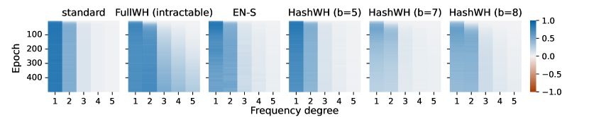
(a) $\text{Train size}=100$

(b) $\text{Train size}=200$

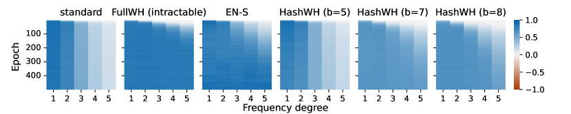
(c) $\text{Train size}=300$

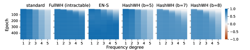
(d) $\text{Train size}=400$

Figure 6: Evolution of the Fourier spectrum during training limited to the target support, using training sets of different sizes. All synthetic functions have single frequencies of each degree in their support that are all given the amplitude of $1$. This is an extended version of Figure 1(a), where we only reported the results for the train set size $200$. It can be observed that the Fourier-sparsity-inducing (regularized) methods are always better than the standard neural network in picking up the higher-degree frequencies, regardless of the training size. Each method shows better performance when trained on a larger training set in terms of converging at earlier epochs and also converging to the true Fourier amplitude it is supposed to.

We randomly generated five synthetic target functions $g^{*}\in\{0,1\}^{10}$ of degree $d=5$, each having a single frequency of each degree in its support (the randomness is over the choice of support). We create a dataset by randomly sampling the Boolean cube. Figure 6 shows the evolution of the Fourier spectrum of the learned neural network function for different methods over training on datasets of multiple sizes ($100,200,300,400$) limited to the target support. This is the extended version of Figure 1(a), where we only reported results for the train size of $200$. We observe that, quite unsurprisingly, each method shows better performance when trained on a larger training set in terms of converging at earlier epochs and also converging to the true Fourier amplitude it is supposed to. It can also be observed that the Fourier-sparsity-inducing (regularized) methods are always better than the standard neural network in picking up the higher-degree frequencies, regardless of the training size.

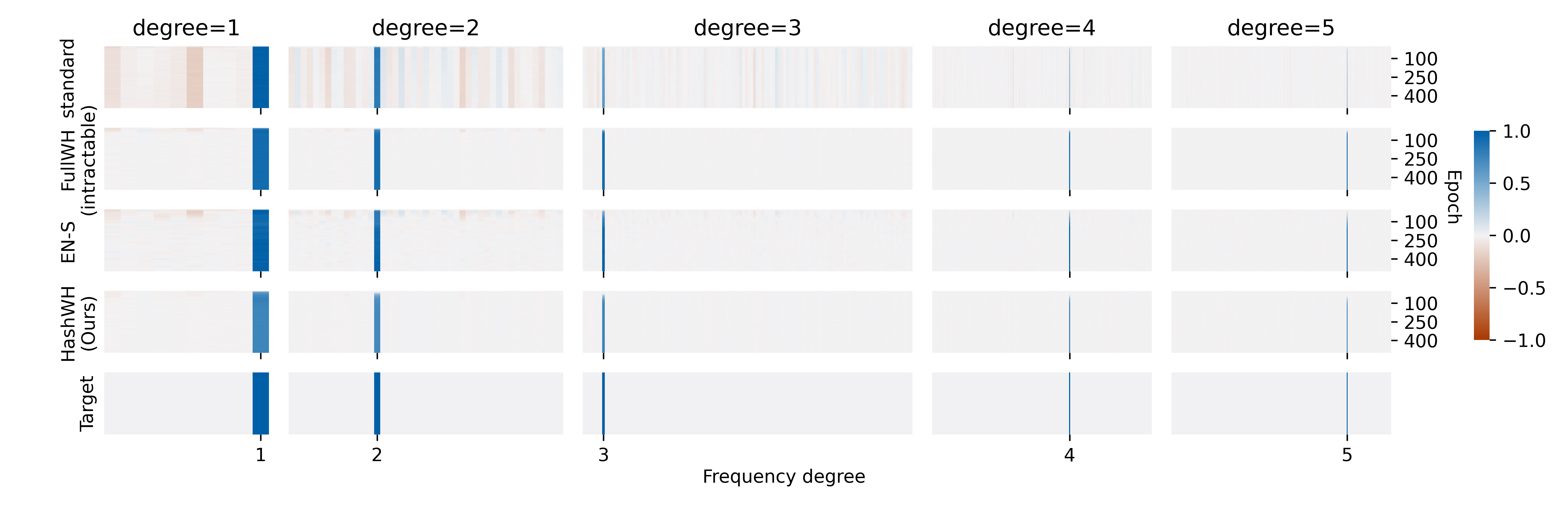
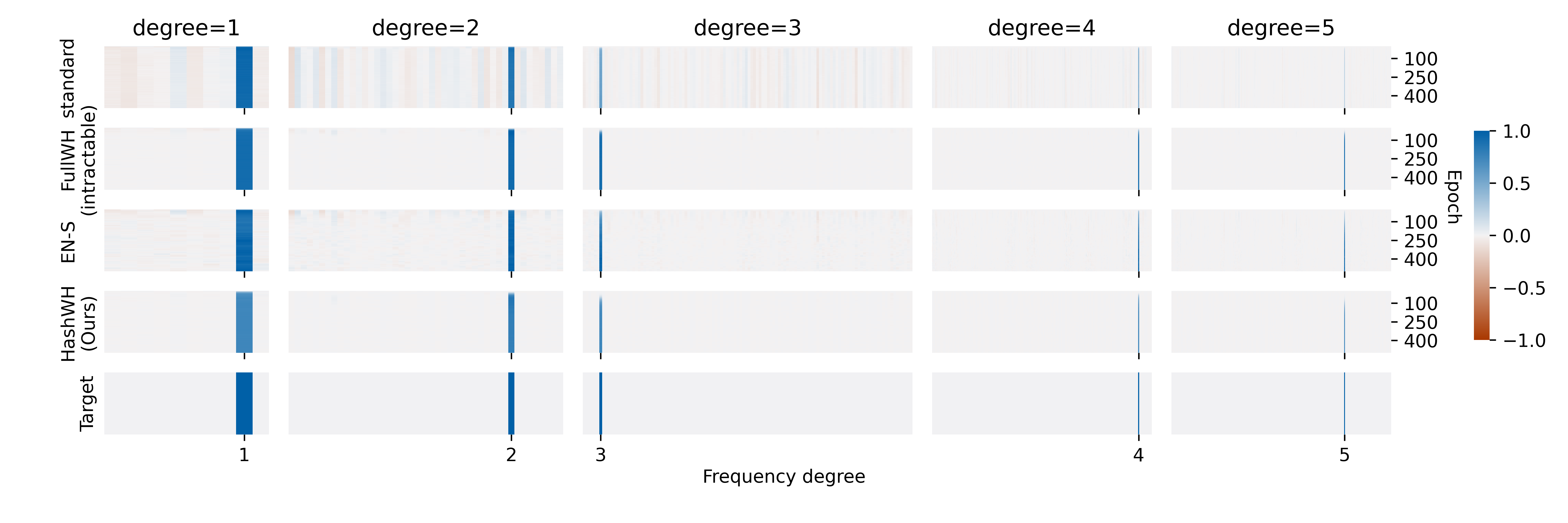
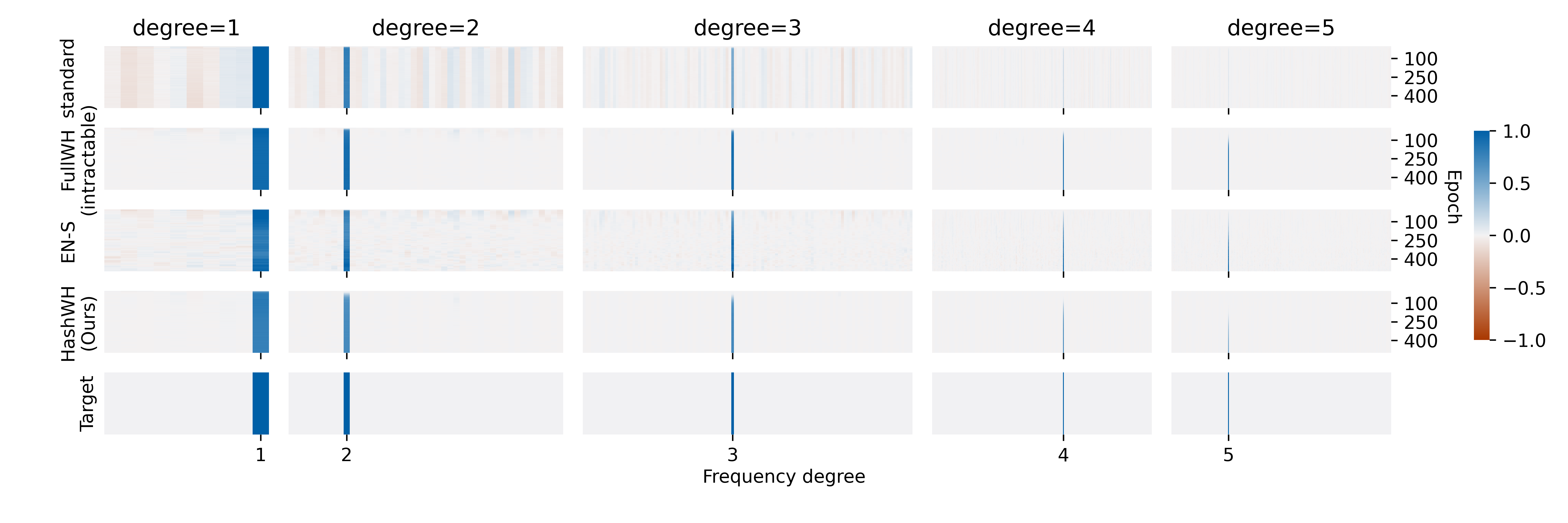
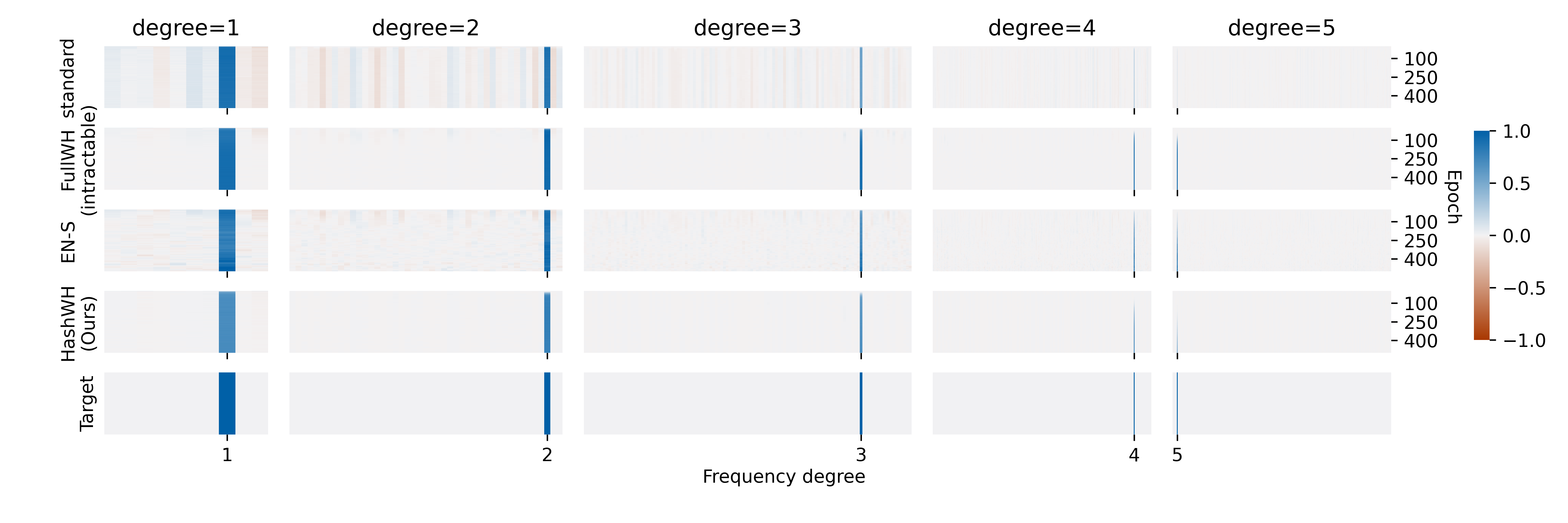
Figure 7: Evolution of the Fourier spectrum in learning a synthetic function $g^{*}\in\{0,1\}^{10}$ of degree $5$ during training, categorized by frequency degree. All synthetic functions used have single frequencies of each degree in their support that are all given the amplitude of $1$. We reported the results for one draw of $g^{*}$ in Figure 1(b) and the four others here, for the training dataset size of $200$. In addition to the incapability of the standard neural network in learning high-degree frequencies, they tend to consistently pick up wrong low-degree frequencies. Both of the problems are remedied through our regularizer.

Figure 7 goes a step further and shows the evolution of the full Fourier spectrum (not just the target frequencies) over the course of training. Here, unlike the previous isolated setting where we were able to aggregate the results from different target functions (because of always having a single frequency of each degree in the support), we have to separate the results for each target function $g^{*}\in\{0,1\}^{10}$, as each has a unique set of frequencies in its support. In Figure 1(a), we reported the results for one version of the target function $g^{*}$ and Figure 7 shows the Fourier spectrum evolution for the other four. We observe that in addition to the spotted inability of the standard neural network in learning higher-degree frequencies, it seems to start picking up erroneous low-degree frequencies as well.

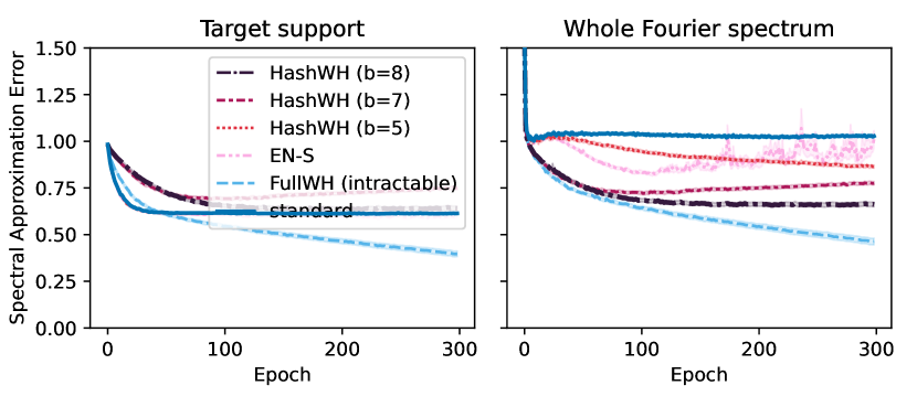
(a) $\text{Train size}=100$

(b) $\text{Train size}=200$

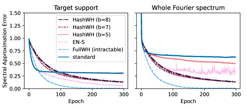
(c) $\text{Train size}=300$

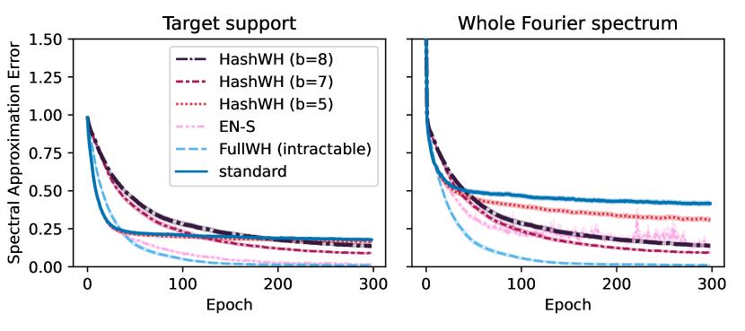
(d) $\text{Train size}=400$

Figure 10: Evolution of the spectral approximation error (SAE) during training. The left plot limits the error to the target support, while the right one considers the whole Fourier spectrum. This is an extended version of Figure 2, where we only reported results for train size $200$. The standard neural network is able to achieve a lower (better) (train size $100$) or somewhat similar (train size $400$) SAE on the target support compared to our method. However, our method always achieves lower SAE on the whole Fourier spectrum, regardless of $b$ used. This shows how our regularisation method is effective in preventing the network from learning the wrong frequencies that are not in the support.

To quantitatively validate our findings, in Figure 10, we show the evolution of Spectral Approximation Error (SAE) during training on both target support and the whole Fourier spectrum. This is an extended version of Figure 2, where we report the results for the train size of $200$. Here we also include results when using training datasets of three other train sizes $\{100,300,400\}$. We observe that even though the standard neural network exhibits comparable performance to HashWH on the target support when the training dataset size is $100$ and $400$, it is always underperforming HashWH when broadening our view to the whole Fourier spectrum, regardless of the train size and the hashing size.

From a more fine-grained perspective, in Figure 9, we categorize the frequencies into subsets of the same degree and show the evolution of SAE and energy on each individual degree. This is an extended version of Figure 3, where we reported the results for the training dataset size of $200$. Firstly, we observe that using more data aids the standard neural network to eventually put more energy on higher-degree frequencies. But it is still incapable of appropriately learning higher-degree frequencies. Fourier-sparsity inducing methods, including ours, show significantly higher energy in the higher degrees. Secondly, No matter the train size, we note that the SAE on low-degree frequencies first decreases and then increases and the standard neural network starts to overfit. This validates our previous conclusion that the standard neural network learns erroneous low-degree frequencies. Our regularizer prevents overfitting in lower degrees. Its performance of which can be scaled using the hashing size parameter $b$.

F.2 High-dimensional synthetic data

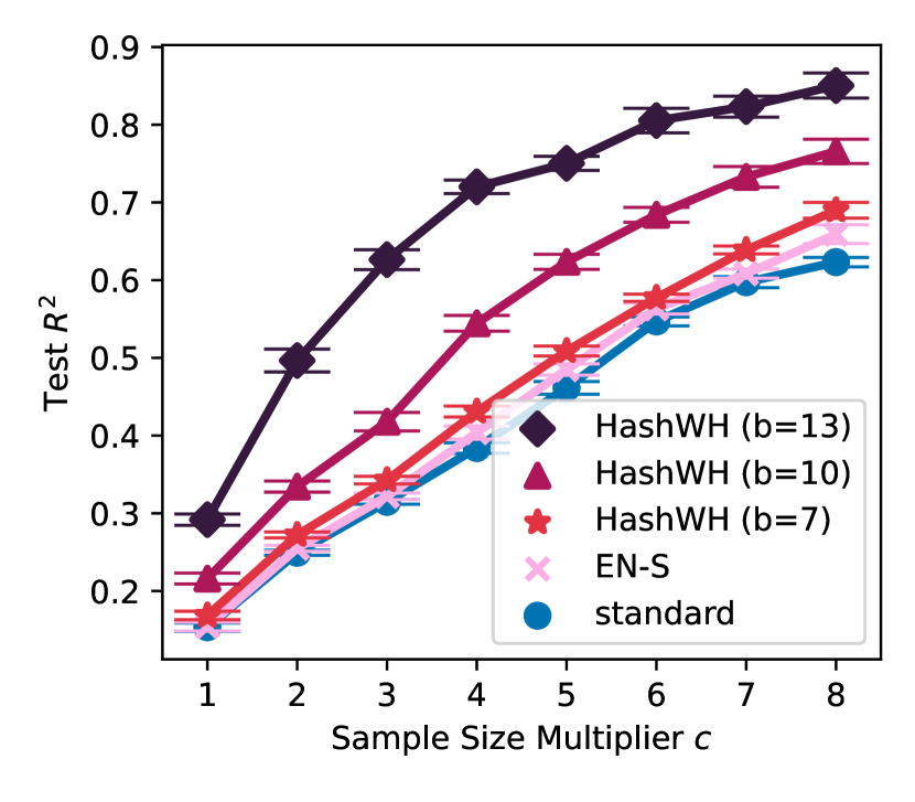
(a) $n=25$, first draw of $g^{*}$

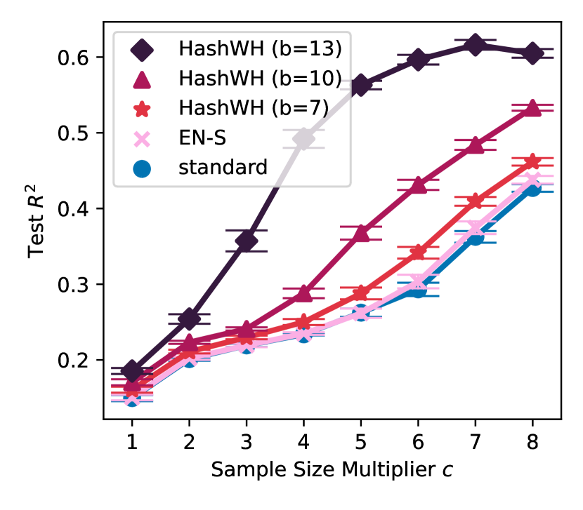
(b) $n=25$, second draw of $g^{*}$

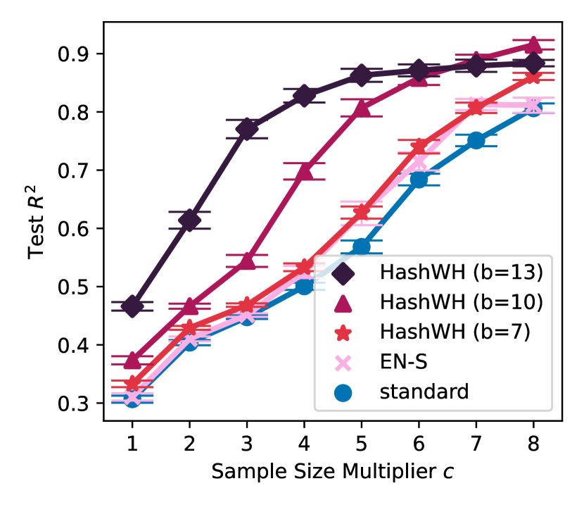
(c) $n=25$, third draw of $g^{*}$

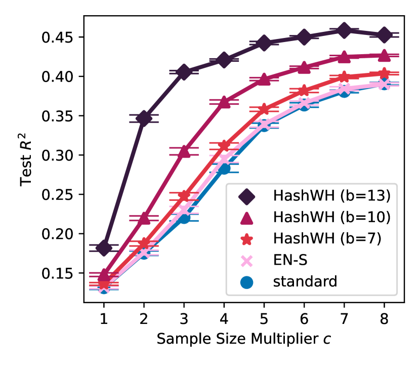
(d) $n=50$, first draw of $g^{*}$

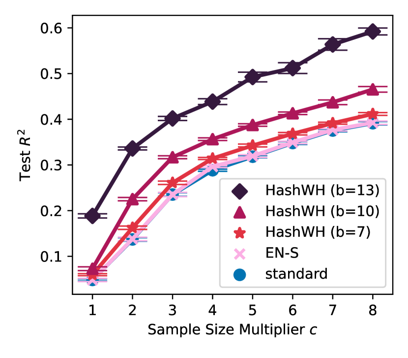
(e) $n=50$, second draw of $g^{*}$

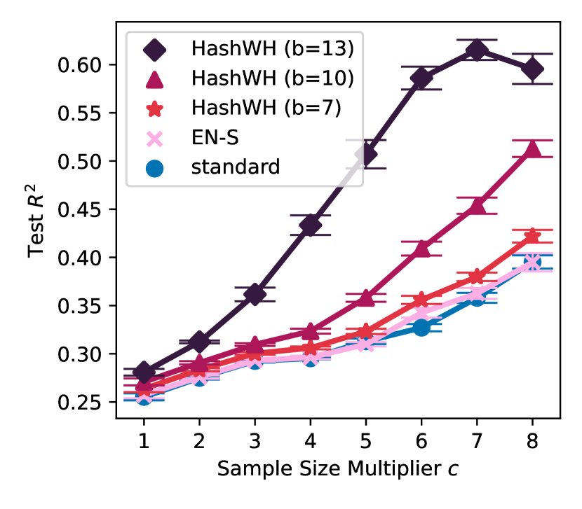
(f) $n=50$, third draw of $g^{*}$

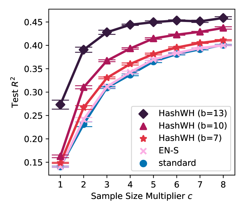
(g) $n=100$, first draw of $g^{*}$

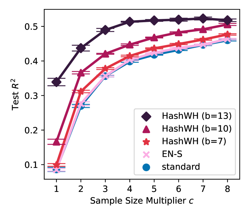
(h) $n=100$, second draw of $g^{*}$

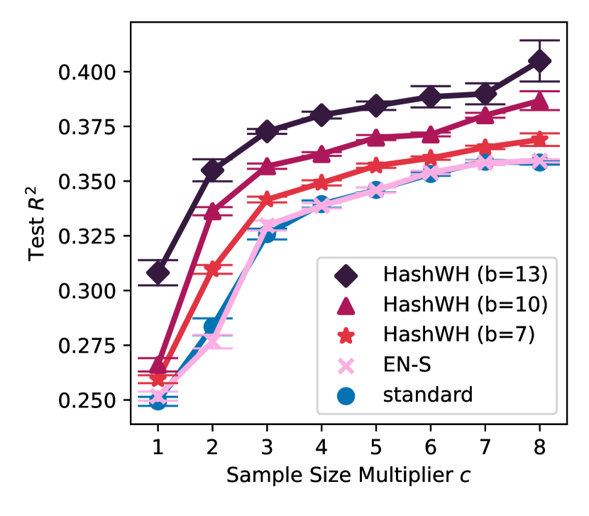
(i) $n=100$, third draw of $g^{*}$

Figure 11: Generalization performance $R^{2}$ on a hold-out test set, in learning a synthetic degree $5$ function $g^{*}\in\{0,1\}^{n}$ for $n\in\{25,50,100\}$, using datasets of size $c\cdot 25n$. We report the results of the first draws of $g^{*}$ for each input dimension in Figure 4(a) and the extended version for all three draws of $g^{*}$ of different dimensions here. Our method, HashWH, always outperforms the standard neural network and EN-S. We are capable of significantly increasing the outperformance margin by increasing $b$. EN-S, however, does not show improvement over the standard network in most cases which indicates its diminishing effectiveness as the size of the input dimension grows, i.e., the number of features increases.

Figure 11 shows the generalization performance of different methods in learning a synthetic degree $d=5$ function $g^{*}\in\{0,1\}^{n}\rightarrow\mathbb{R}$, for $n\in\{25,50,100\}$, using train sets of different sizes ($c\cdot 25n,c\in[8]$). For each $n$ we sample three different draws of $g^{*}$. This is the extended version of Figure 4(a), where we only reported the results for the first draw of $g^{*}$ for each input dimension $n$. Our regularization method, HashWH, outperforms the standard network and EN-S in all possible combinations of input dimension and dataset sizes, regardless of the draw of $g^{*}$. We observe that increasing $b$ in HashWH, i.e. increasing the number of hashing buckets, almost always improves the generalization performance. EN-S, on the other hand, does not show significant superiority over the standard neural network rather than marginally outperforming it in a few cases when $n=25$. This does not match its performance in the previous section and conveys that it is not able to perform well when increasing the input dimension, i.e., having more features in the data.

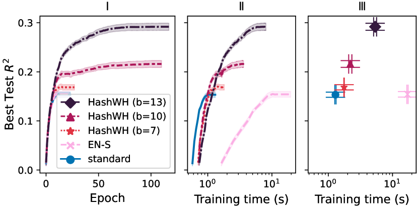
(a) $n=25$, $c=1$

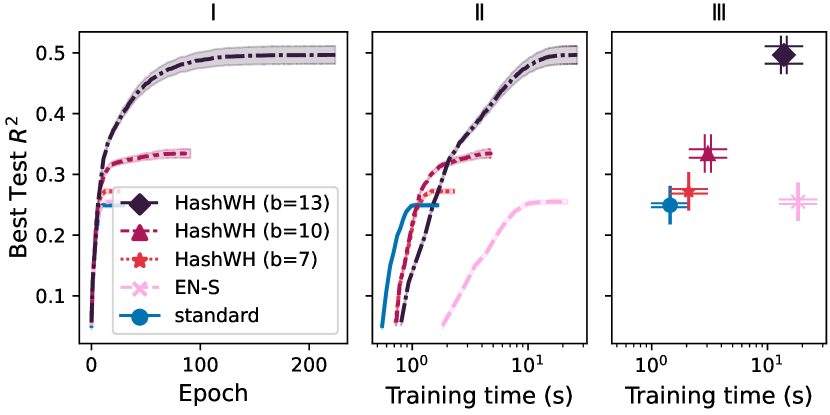
(b) $n=25$, $c=2$

(c) $n=25$, $c=3$

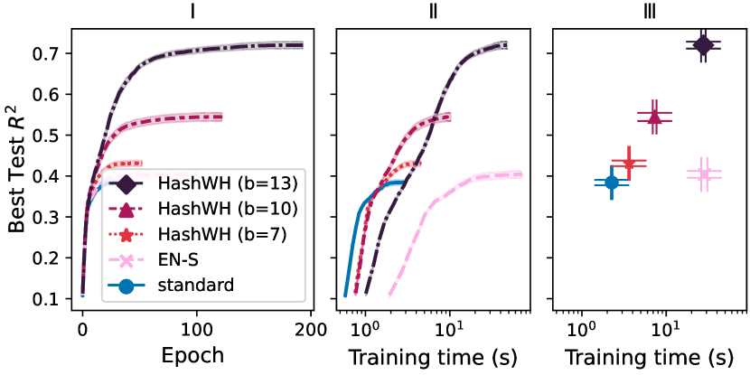
(d) $n=25$, $c=4$

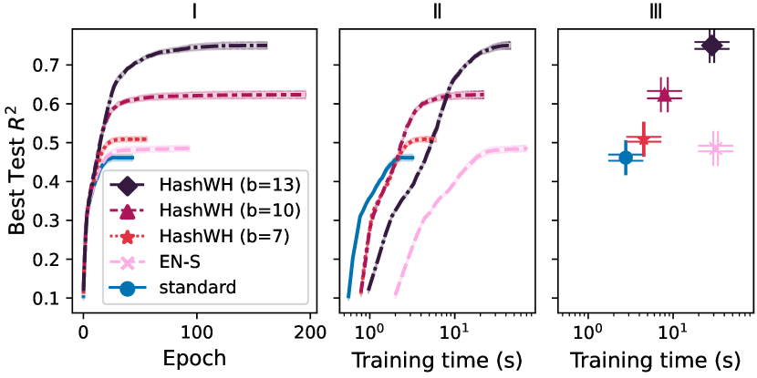
(e) $n=25$, $c=5$

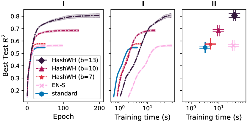
(f) $n=25$, $c=6$

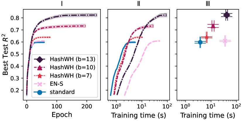
(g) $n=25$, $c=7$

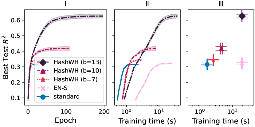
(h) $n=25$, $c=8$

Figure 12: Best achievable generalization performance $R^{2}$ up to a certain epoch or training time (seconds), in learning a synthetic degree $5$ function $g^{*}\in\{0,1\}^{n}$, using datasets of size $c\cdot 25n$. This figure is an extended version of Figure 4(b), where we reported similar plots for $n=50$ and $c=5$. Here we report the results for the first draw of $g^{*}$ with $n=25$. Our method, HashWH, always outperforms EN-S $R^{2}$ score in significantly less time. HashWH can also be scaled by the choice of $b$ to achieve better generalization performance at th price of higher training times.

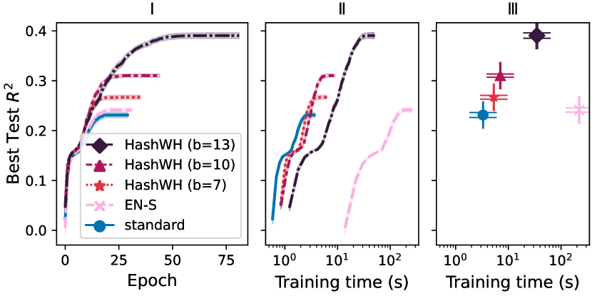
(b) $n=50$, $c=2$

(c) $n=50$, $c=3$

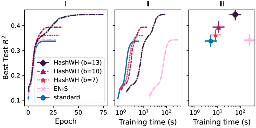
(d) $n=50$, $c=4$

(e) $n=50$, $c=5$

(f) $n=50$, $c=6$

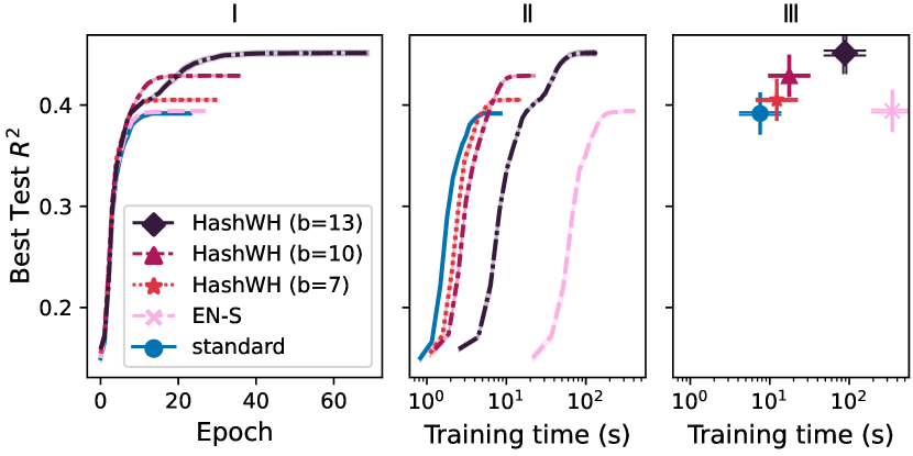
(g) $n=50$, $c=7$

(h) $n=50$, $c=8$

Figure 13: Best achievable generalization performance $R^{2}$ up to a certain epoch or training time (seconds), in learning a synthetic degree $5$ function $g^{*}\in\{0,1\}^{n}$, using datasets of size $c\cdot 25n$. This figure is an extended version of Figure 4(b), where we reported similar plots for $n=50$ and $c=5$. Here we report the results for the first draw of $g^{*}$ with $n=50$. Our method, HashWH, always outperforms EN-S $R^{2}$ score in significantly less time. HashWH can also be scaled by the choice of $b$ to achieve better generalization performance athe price of higher training times.

To both showcase the computational scalability of our method, HashWH, and compare it to EN-S, we show the achievable performance by the number of training epochs and training time in Figures 12, 13 and 14, for all train set sizes and input dimensions individually and limited to the first draw of $g^{*}$ for each input dimension. This is the extended version of Figure 4(b) where we only reported it for $n=50$ and the sample size multiplier $c=5$. We consistently see that the trade-off between the generalization performance and the training time can be directly controlled in HashWH using the parameter $b$. Furthermore, HashWH is able to always exhibit a significantly better generalization performance in remarkably less time, in all versions of $b$ tested. This emphasizes the advantage of our method in not directly computing the approximate Fourier spectrum of the network, which resulted in this gap with EN-S in the run time, that increases as the input dimension $n$ grows.

F.3 Real data

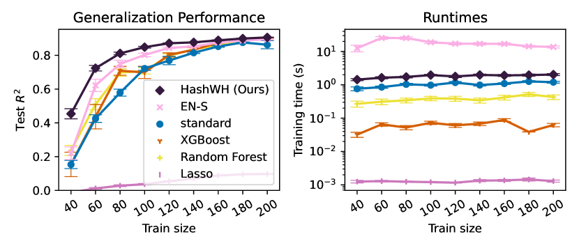
(a) Entacmaea (n=13)

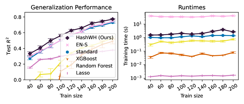
(b) SGEMM (n=40)

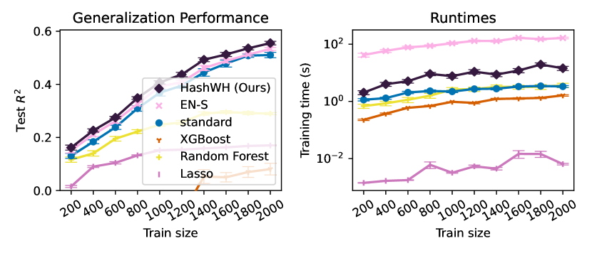
(c) GB1 (n=80)

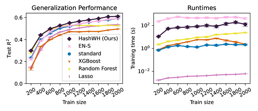
(d) avGFP (n=236)

Figure 15: Generalization performance of standard/regularized neural networks and benchmark ML models on four real datasets. This figure is an extended version of Figure 5. It also includes the training times (logarithmically scaled in the plot). Our method is able to achieve the best test $R^{2}$s while always training significantly faster than EN-S.

Figure 15 shows the generalization performance and the training time of different methods, including relevant machine learning benchmarks, in learning four real datasets. It is the extended version of Figure 5, where we only reported the generalization performance and not the training time. The training time for neural nets is considered to be the time until overfitting occurs i.e. we do early stopping. In addition to superior generalization performance of our method, HashWH, in most settings, again, we see that it is able to achieve it in significantly less time than EN-S. Lasso is the fastest among the methods but usually shows poor generalization performance.

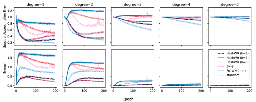
(a) $\text{Train size}=100$

(b) $\text{Train size}=200$

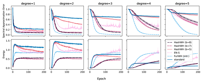
(c) $\text{Train size}=300$

Figure 8: Evolution of the Spectral Approximation Error (SAE) and energy of the network during training, categorized by frequency degree (continued in the next page).

(a) $\text{Train size}=400$

Figure 9: Evolution of the Spectral Approximation Error (SAE) and energy of the network during training, categorized by frequency degree. This is an extended version of Figure 3, where we only reported results for training dataset size $200$. Firstly, in a standard neural network, the energy is mostly put on low-degree frequencies as compared to the high-degree frequencies. The energy slightly shifts towards high-degree frequencies when increasing the training dataset size. Our regularizer facilitates the learning of higher degrees in all cases. Secondly, over the lower-degree and regardless of the train size, the standard neural network’s energy continues to increase while the SAE first decreases then reverts and increases. This shows that the standard neural network emphasizes energy on erroneous low-degree frequencies and overfits. Our regularizer prevents overfitting in lower degrees.

(a) $n=50$, $c=1$

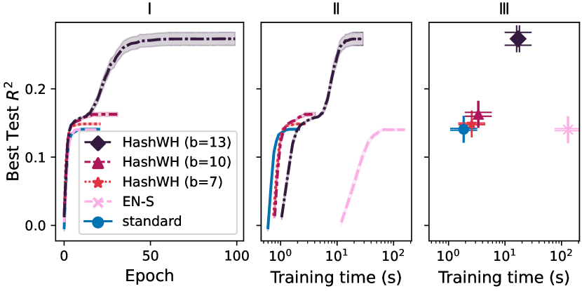
(a) $n=100$, $c=1$

(b) $n=100$, $c=2$

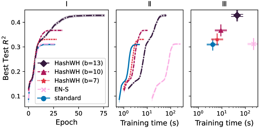
(c) $n=100$, $c=3$

(d) $n=100$, $c=4$

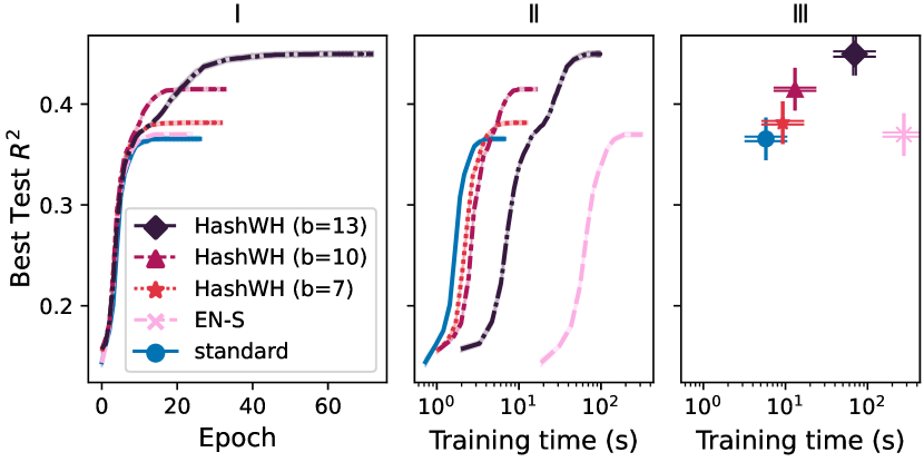
(e) $n=100$, $c=5$

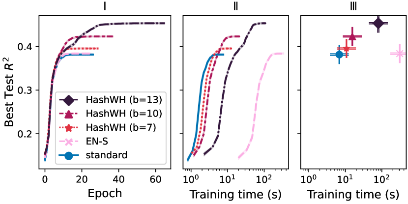
(f) $n=100$, $c=6$

(g) $n=100$, $c=7$

(h) $n=100$, $c=8$

Figure 14: Best achievable generalization performance $R^{2}$ up to a certain epoch or training time (seconds), in learning a synthetic degree $5$ function $g^{*}\in\{0,1\}^{n}$, using datasets of size $c\cdot 25n$. This figure is an extended version of Figure 4(b), where we reported similar plots for $n=50$ and $c=5$. Here we report the results for the first draw of $g^{*}$ with $n=100$. Our method, HashWH, always outperforms EN-S $R^{2}$ score in significantly less time. HashWH can also be scaled by the choice of $b$ to achieve better generalization performance at the price of higher training times.