The HI intensity mapping power spectrum:
insights from recent measurements

Abstract

The first direct measurements of the HI intensity mapping power spectrum were recently made using the MeerKAT telescope. These measurements are on nonlinear scales, at redshifts 0.32 and 0.44. We develop a formalism for modelling small-scale power in redshift space, within the context of the mass-weighted HI halo model framework. This model is consistent with the latest findings from surveys on the HI-halo mass relation. In order to model nonlinear scales, we include the 1-halo, shot-noise and finger-of-god effects. Then we apply the model to the MeerKAT auto-correlation data, finding that the model provides a good fit to the data at redshift 0.32, but the data may indicate some evidence for an adjustment at $z\sim 0.44$. Such an adjustment can be achieved by an increase in the HI halo model bias.

1 Introduction

The clustering of dark matter haloes and their tracers is usually described by its two-point correlation function and the associated power spectrum. The small-scale structure of the power spectrum contains valuable information about baryonic effects and peculiar velocities which is useful for breaking degeneracies in cosmological parameters. Intensity mapping of neutral hydrogen (HI), a key tracer of cosmological dark matter, promises stringent constraints on the abundances and clustering of dark matter and baryons on cosmological scales. So far, most studies focused on HI intensity mapping in cross-correlation with galaxy surveys using single-dish telescopes (e.g., Chang et al., 2010; Masui et al., 2013; Switzer et al., 2013; Anderson et al., 2018; Wolz et al., 2022) or telescope arrays operating in single-dish mode (e.g. Cunnington et al., 2023). The first direct detection and measurement of the HI intensity mapping auto-correlation fluctuations was recently made with the MeerKAT interferometer by Paul et al. (2023), on nonlinear scales $0.4<k\leq 8\,{\rm Mpc}^{-1}$.

In parallel, there has been recent progress on using stacked individual galaxy detections in HI to understand the properties of the baryon cycle out to $z\sim 0.3-1$, using the Giant Metrewave Radio Telescope (GMRT; Bera et al., 2019, 2022) and the MeerKAT MIGHTEE survey (Sinigaglia et al., 2022). The results show that HI may play a significant role in the star formation process at these redshifts.

Previous work (Padmanabhan et al., 2017; Padmanabhan & Refregier, 2017) has built a framework connecting the abundance and clustering of HI to that of dark matter in a data-driven manner, analogous to the halo model developed for the latter. In this framework, the small-scale structure of HI is modelled using the one-halo term of the power spectrum, without considering the effect of peculiar velocities that alter the form of the power spectrum via redshift-space distortions (RSD). The RSD ‘finger-of-god’ effects are especially important on nonlinear scales. Theoretical prescriptions to model RSD in the context of HI have been applied to both hydrodynamical simulations (Villaescusa-Navarro et al., 2018) and semi-analytic treatments populating HI in dark matter simulations (Sarkar & Bharadwaj, 2018).

Preliminary findings from the cross-correlation of an HI intensity map from the Parkes telescope with a galaxy sample from the 2dF survey at $z\sim 0$ (Anderson et al., 2018), confirmed that RSD effects become important at small scales. Padmanabhan (2021) developed expressions for the small-scale structure of HI including redshift space effects, and found them to be a good match to the Parkes-2dF cross-correlation data. In particular, the low amplitude of clustering observed in the results was largely found to be consistent with an exponential finger-of-god suppression of power, within the HI halo-model framework.

Here, we expand upon the details of the derivation, formulating approximations for the RSD treatment in the halo-model framework for a generic, mass-weighted tracer. We fix the parameters of the model to the best-fit values from stacking data, and we use a weighted average model for the finger-of-god damping parameter, following Zhang et al. (2020). Then we apply our model to the recent MeerKAT data on small scales. We find that at $z=0.32$, the model provides a good fit to the data, including the small scale structure of the power spectrum. At the higher redshift interval centred at $z=0.44$, the data may indicate evidence for a higher-than expected amplitude of the power spectrum compared to theoretical predictions. Such an increase may have different possible causes, including higher order biases or more complex baryonic effects. We also predict the two-dimensional power spectra at these redshifts from the formalism thus developed.

The paper is organised as follows. In Section 2, we establish the notation and review the formalism for modelling the redshift-space power spectrum for dark matter in the halo model. We review the main ingredients involved in formulating the halo model for HI (and in general, a biased mass-weighted tracer of dark matter) in Section 3, including the one-halo and shot noise terms which describe effects on small scales. We also compare the halo model predictions to recent results from the stacking of HI galaxies (Bera et al., 2022) and intensity mapping auto-correlation power spectra (Paul et al., 2023). In Section 4, we formulate the treatment of RSD in the monopole of the HI power spectra analytically, and compare these to the MeerKAT results at $z=0.32$ and $z=0.44$. We then develop expressions for the two-dimensional power spectra in this framework in Appendix A. We summarise our results and discuss the outlook in the concluding Section 5.

2 Fitting parameters for the halo power spectrum in redshift space

We need to model the small-scale behaviour of the HI intensity power spectrum, including RSD. In the halo-model formalism, the halo power spectrum is split into a 1-halo (correlations within the same dark matter halo) and a 2-halo (correlation between perturbations in distinct halos) term (see Cooray & Sheth, 2002, for a review):

$$P_{\rm h}(k)=P_{\rm 1h}{(k)}+P_{\rm 2h}{(k)}\;,$$ (1)

where

$$P_{\rm 1h}{(k)} =\frac{1}{\bar{\rho}_{\rm m}^{2}}\int\mbox{d}M\,n(M)M^{2}|u_{\rm h}(k|M)|^{2}\;,$$ (2)

$$P_{\rm 2h}{(k)} =P_{\rm lin}(k)\Big{[}\frac{1}{\bar{\rho}_{\rm m}}\int\mbox{d}M\,n(M)Mb(M)\big{|}u_{\rm h}(k|M)\big{|}\Big{]}^{2}.$$ (3)

Here $\bar{\rho}_{\rm m}$ is the average dark matter density, $M$ is the halo mass, $n$ is the halo mass function, $u_{\mathrm{h}}$ is the Fourier transform of the mass density profile, $P_{\rm lin}(k)$ is the linear matter power spectrum, and $b$ is the halo bias. In the above equations and elsewhere we have omitted the redshift dependence for brevity.

Since observations make measurements of positions in redshift space, we modify the power spectra by following, e.g. the treatments in Seljak (2000), White (2001), and Peacock & Dodds (1994). The position of a halo in redshift space is

$$\bm{s}=\bm{x}+\frac{\bm{v}\cdot\hat{\bm{n}}}{a\,H}\,\hat{\bm{n}}\;,$$ (4)

where $\bm{x}$ is the position in real space, $\bm{v}\cdot\hat{\bm{n}}$ is the velocity component along the line-of-sight direction $\hat{\bm{n}}$ (assumed to be fixed), and $H$ is the Hubble rate at scale factor $a$. As a result, the halo density field in Fourier space, $\delta_{\rm h}$, acquires a correction of the form

$$\delta_{\rm h}^{\rm s}(\bm{k})=\delta_{\rm h}(\bm{k})\Big{(}1+f\mu^{2}\Big{)}\exp\Big{(}-\frac{1}{2}k^{2}\mu^{2}\sigma^{2}\Big{)},$$ (5)

made up of a Kaiser (Kaiser, 1987) and a finger-of-god term, where

$$k=|\bm{k}|=\Big{(}{k_{\parallel}^{2}+\bm{k}_{\perp}^{2}}\Big{)}^{1/2}\,,~{}~{}\mu=\hat{\bm{k}}\cdot\hat{\bm{n}}=\frac{k_{\parallel}}{k}\,,~{}~{}f=\frac{\mbox{d}\ln D}{\mbox{d}\ln a}\,.$$ (6)

Here $D$ is the linear growth factor whose growth rate can be well approximated as $f(a)\simeq{[\Omega_{\mathrm{m}}(a)]^{0.55}}$. The finger-of-god damping is described by a Gaussian (exponential) suppression, where $\sigma$ is the pairwise velocity dispersion (which is a function of halo mass and redshift).

Then the RSD power spectrum is $P_{\rm h}^{\rm s}=P^{\rm s}_{\rm 1h}+P^{\rm s}_{\rm 2h}$, where

$$P^{\rm s}_{\rm 1h}(k,\mu) =\frac{\big{(}1+f\mu^{2}\big{)}^{2}}{\bar{\rho}_{\rm h}^{2}}\!\int\!\mbox{d}Mn(M)M^{2}\big{|}u_{\rm h}(k|M)\big{|}^{2}{\rm e}^{-k^{2}\mu^{2}\sigma^{2}},$$ (7)

$$P^{\rm s}_{\rm 2h}(k,\mu) =P_{\rm lin}(k)\bigg{[}\frac{\big{(}1+f\mu^{2}\big{)}}{\bar{\rho}_{\rm h}}$$

$$~{}~{}~{}\times\int\!\mbox{d}Mn(M)Mb_{\rm h}(M)\big{|}u_{\rm h}(k|M)\big{|}\,{\rm e}^{-k^{2}\mu^{2}\sigma^{2}/2}\bigg{]}^{2}\!.$$ (8)

The monopole is the average power spectrum ${\bar{P}}_{\rm h}^{\rm s}=\int\mbox{d}\mu\,P_{\rm h}^{\rm s}/2$, which leads to:

$$\bar{P}^{\rm s}_{\rm 1h}(k) =\frac{1}{\bar{\rho}_{\rm h}^{2}}\int\mbox{d}M\,n(M)M^{2}\big{|}u_{\rm h}(k|M)\big{|}^{2}\ \mathcal{R}_{1}(k\sigma),$$ (9)

$$\bar{P}^{\rm s}_{\rm 2h}(k) \simeq\left(1+\frac{2}{3}f+\frac{1}{5}f^{2}\right)P_{\rm lin}(k)$$

$$~{}~{}~{}\times\left[\frac{1}{\bar{\rho}_{\rm h}}\int\mbox{d}M\,n(M)Mb_{\rm h}(M)\mathcal{R}_{2}(k\sigma)\big{|}u_{\rm h}(k|M)\big{|}\right]^{2}.$$ (10)

The functions ${\cal R}_{i}$ are given by

$${\cal R}_{1}(y) =\frac{1}{2}\int_{-1}^{1}\mbox{d}\mu\left(1+f\mu^{2}\right)^{2}{\rm e}^{-{y}^{2}\mu^{2}}=\frac{\sqrt{\pi}}{8}\,\frac{{\rm erf}(y)}{y^{5}}\,\Big{[}3f^{2}+$$

$$~{}~{}~{}~{}~{}4fy^{2}+4y^{4}\Big{]}-\frac{{\rm e}^{-y^{2}}}{4y^{4}}\Big{[}f^{2}\big{(}3+2y^{2}\big{)}+4fy^{2}\Big{]},$$ (11)

$${\cal R}_{2}(y) =\frac{1}{2}\int_{-1}^{1}\mbox{d}\mu\,{\rm e}^{-{y}^{2}\mu^{2}/2}=\sqrt{\frac{\pi}{2}}\,\frac{{\rm erf}(y/\sqrt{2}\,)}{y}.$$ (12)

Note that the $M$-dependence in ${\cal R}_{i}$ comes from the $\sigma$ term. Similar expressions hold for the Lorentzian finger-of-god damping factor.

3 Halo model for HI and its parametrisation

We now extend this formalism to describe the small-scale structure of the power spectrum of a mass-weighted tracer. In the case of HI, we start with the formalism connecting HI mass to the underlying dark matter halo mass, given by (Padmanabhan et al., 2017)

$$M_{\rm HI}(M,z)=\alpha f_{\rm H,c}M\left(\frac{M}{10^{11}\,h^{-1}{\rm M}_{\odot}}\right)^{\beta}\!\exp\left\{\!-\left[\frac{v_{{\rm c},0}}{v_{\rm c}(M,z)}\right]^{3}\right\},$$ (13)

with the three free parameters $\alpha$, $\beta$ and $v_{\rm c,0}$ describing the overall normalization, logarithmic slope and lower virial velocity cutoff of the dark matter halo hosting HI, respectively. Their best-fitting values and $1\sigma$ uncertainties, constrained by a joint fit to the available HI data including DLAs and HI galaxy surveys (Padmanabhan & Refregier, 2017; Padmanabhan et al., 2017), were found to be given by:

$$\alpha=0.09\pm 0.01,~{}\beta=-0.58\pm 0.06,~{}\log_{10}\Big{[}\frac{v_{{\rm c},0}}{1\,\mathrm{km/s}}\Big{]}=1.56\pm 0.04.$$ (14)

We compare the HI mass – halo mass relation predicted by the halo model to recent observations in Fig. 1. We consider two recent surveys targeting HI in galaxy surveys and intensity mapping at $z\sim 0.3-0.4$: (1) the MeerKAT survey (Paul et al., 2023), in which HI is probed down to very small scales, $k\sim 10\,h\,\mathrm{Mpc}^{-1}$; and (2) recent results probing stacked 21 cm emission in star-forming galaxies at $z\sim 0.35$ from the Giant Metrewave Radio Telescope (GMRT) Extended Goth Strip (EGS) survey (Bera et al., 2019, 2022). These and recent results probing HI in the $z\sim 1$ range (Chowdhury et al., 2021, 2022) suggest that HI may evolve strongly over $z\sim 0-1$ and even contribute a major fraction of fuel for the star-formation.

The mass functions from both surveys, denoted by $\phi(M_{\rm HI})$, are used to constrain the HI mass -halo mass relation via the abundance matching technique (e.g. Padmanabhan & Kulkarni, 2017), which assumes a monotonicity between the HI mass and the underlying halo mass:

$$\int_{M(M_{\rm HI})}^{\infty}\mbox{d}\log_{10}\!M\,\frac{\mbox{d}n}{\mbox{d}\log_{10}\!M}=\int_{M_{\rm HI}}^{\infty}\mbox{d}\log_{10}\!M_{\rm HI}\,\phi(M_{\rm HI})\;.$$ (15)

Figure 1 shows that the current halo model parameters (green curve) are consistent with the latest MeerKAT findings (blue curve), while the stacking results (orange curve) show a steeper drop at low HI masses. This is in line with theoretical expectations, since the stacking results target individual galaxies while the MeerKAT result additionally measures the overall or integrated emission from lower luminosity sources.

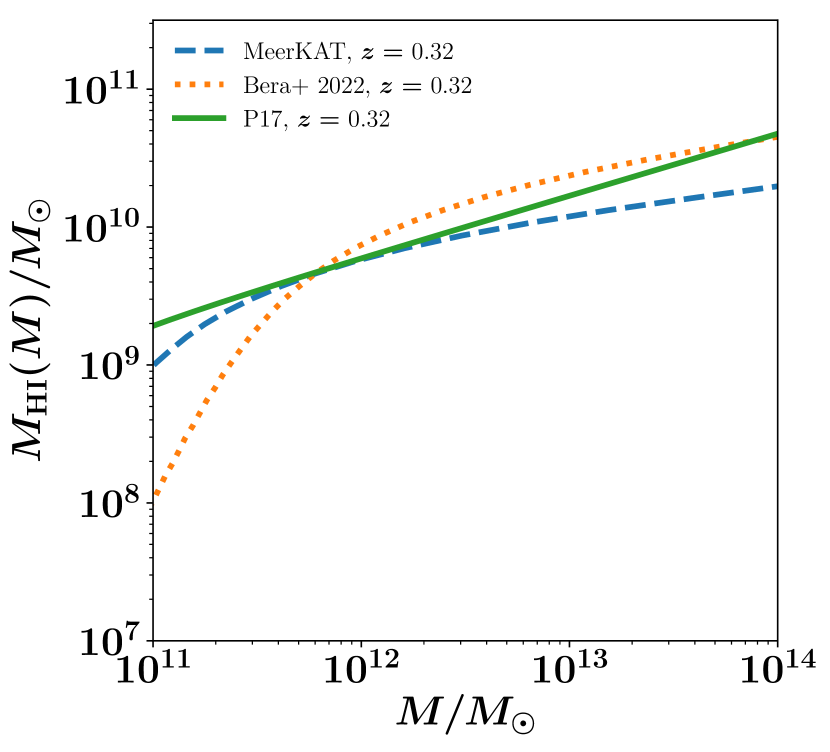
Figure 1: Halo model predictions for the average HI mass - halo mass relation at $z=0.32$ (green solid line), compared to the relation inferred from abundance matching the findings of the MeerKAT intensity mapping observations (Paul et al., 2023) (blue dashed line) and the galaxy stacking results of Bera et al. (2022) (orange dotted line).

The small-scale structure of HI is encoded in the density profile, given by

$$\rho_{\rm HI}(r,M,z)=\rho_{0}\,\exp\left[-\frac{r}{r_{\rm s}(M,z)}\right]\;,$$ (16)

in which $r_{\rm s}$ is the scale radius of the halo, and defined as $r_{\rm s}(M,z)\equiv R_{\rm v}(M)/c_{\rm HI}(M,z)$. Here, $R_{\rm v}(M)$ denotes the virial radius of a halo of mass $M$, and $c_{\rm HI}$ the concentration of the HI, analogous to the corresponding expression for dark matter, defined as (Macciò et al., 2007)

$$c_{\rm HI}(M,z)=c_{{\rm HI},0}\left(\frac{M}{10^{11}\,{\rm M}_{\odot}}\right)^{-0.109}\frac{4}{(1+z)^{\gamma}}\;.$$ (17)

The constant of proportionality in Eq. 16, denoted by $\rho_{0}$, is found by normalising the HI mass within the virial radius $R_{\rm v}(M,z)$ at a given halo mass and redshift to $M_{\rm HI}$. This can be shown to be well approximated by

$$\rho_{0}(M,z)=\frac{M_{\rm HI}(M)}{8\pi r_{\rm s}(M,z)^{3}}\;.$$ (18)

The radial density profile thus introduces two more free parameters: the normalization of the concentration, $c_{\rm HI,0}$, and its redshift-dependent slope, $\gamma$. The best-fitting values of these parameters were found to be:

$$c_{\rm HI,0}=28.65\pm 1.76,~{}\gamma=1.45\pm 0.04$$ (19)

in the HI halo model framework (Padmanabhan et al., 2017).

Using this parametrised form for the HI-halo mass relation, we compute the power spectrum on both linear and nonlinear scales from

$$P_{\rm 1h,HI}{(k)} =\frac{1}{\bar{\rho}_{\rm HI}^{2}}\,\int\mbox{d}M\,n(M)M_{\rm HI}^{2}\big{|}u_{\rm HI}(k|M)\big{|}^{2},$$ (20)

$$P_{\rm 2h,HI}{(k)} =P_{\rm lin}(k)\!\left[\frac{1}{\bar{\rho}_{\rm HI}}\!\int\!\mbox{d}Mn(M)M_{\rm HI}(M)b_{\rm h}(M)\big{|}u_{\rm HI}(k|M)\big{|}\right]^{2}\!\!,$$ (21)

where the terms are defined analogously to Eqs. 2 and 3. The mean HI density is given by

$$\bar{\rho}_{\rm HI}=\int\mbox{d}M\,n(M)M_{\rm HI}(M)\;,$$ (22)

and the normalised Fourier transform of the HI density profile is given by

$$u_{\rm HI}(k|M)=\frac{4\pi}{M_{\rm HI}(M)}\int_{0}^{R_{\rm v}(M)}\mbox{d}r\,r^{2}\rho_{\rm HI}(r)\,\frac{\sin kr}{kr}\;.$$ (23)

Another contribution to the HI power spectrum on small scales comes from the shot noise (Villaescusa-Navarro et al., 2018):

$$P_{\rm SN}=\frac{1}{\bar{\rho}_{\rm HI}^{2}}\int\mbox{d}M\,n(M)M_{\rm HI}^{2}\;.$$ (24)

This term corresponds to the $k\to 0$ limit of the 1-halo power spectrum, and provides a measure of the Poisson noise coming from the finite number of discrete sources (Seo et al., 2010; Seehars et al., 2016).

Figure 2: Scale-dependent bias of HI obtained from the halo model using Eq. 25, for $0\leq z\leq 5$.

4 Contributions to the power spectrum at small scales

The power spectrum, both in one- and two-dimensional $k$-space, contains information on the HI distribution on small scales. This is made up of the contributions from (1) the shot noise, (2) the one-halo term described in the previous section, and (3) the RSD finger-of-god effects.

The first two effects are modelled as described in the previous section, and reflected in the scale-dependent bias which can be defined by

$$P_{\rm HI}(k)=b_{\rm HI}(k)^{2}\,P_{\rm h}(k)\;,$$ (25)

and is plotted from the halo model framework in Fig. 2 (solid lines) as a function of redshift. On large scales, the bias is nearly scale-independent, while the scale-dependent effects begin to manifest around $k\sim 1\,h\,\mathrm{Mpc}^{-1}$.

We now consider the contributions of RSD affecting the HI distribution on small scales. To do this, we generalise the expressions found in Section 2 to the case of HI in the context of the halo model for a mass-weighted, biased tracer. In the presence of RSD, the density of HI (in Fourier space) is boosted on large scales by the Kaiser term:

$$\delta_{{\rm HI}}^{\rm s}({\bm{k}})=\delta_{{\rm HI}}({\bm{k}})+f\mu^{2}\delta_{{\rm h}}({\bm{k}})\,,$$ (26)

where $f\delta_{{\rm h}}$ denotes the velocity divergence of the dark matter. In order to incorporate the finger-of-god effect on small scales, we damp the previous expression:

$$\delta_{{\rm HI}}^{\rm s}\to\delta_{{\rm HI}}^{\rm s}\exp\left(-\frac{1}{2}k^{2}\mu^{2}\sigma^{2}\right)\,.$$ (27)

Using the three equations above gives the full expression for the anisotropic ($\mu$-dependent) power spectrum of HI:

$$P_{\rm HI}^{\rm s}(k,\mu)= \;\left\langle\left|\delta_{{\rm HI}}(\bm{k})\exp\left(-\frac{1}{2}k^{2}\mu^{2}\sigma^{2}\right)\right|^{2}\right\rangle$$

$$+\left\langle\left|f\mu^{2}\delta_{{\rm h}}(\bm{k})\,\exp\left(-\frac{1}{2}k^{2}\mu^{2}\sigma^{2}\right)\right|^{2}\right\rangle$$

$$+2\left\langle f\mu^{2}\delta_{{\rm{h}}}(\bm{k})\delta_{{\rm HI}}(\bm{k})\exp\left(-k^{2}\mu^{2}\sigma^{2}\right)\right\rangle\,.$$ (28)

Applying the same procedure as for the dark matter only case treated in Section 2, the monopole of the HI power spectrum in redshift space can be expressed by

$$\bar{P}_{\rm HI}^{\rm s}(k) =\left(F_{\rm HI}^{2}+\frac{2}{3}F_{\rm m}F_{\rm HI}+\frac{1}{5}F_{\rm m}^{2}\right)P_{\rm lin}(k)$$

$$+\frac{1}{\bar{\rho}_{\rm HI}^{2}}\int\mbox{d}M\,n(M)M_{\rm HI}^{2}\,{\cal R}_{1}(k\sigma)\big{|}u_{\rm HI}(k,M)\big{|}^{2},$$ (29)

where

$$F_{\rm m} =f\int\mbox{d}M\,n(M)b(M)\,{\cal R}_{2}(k\sigma)u_{\rm h}(k,M),$$ (30)

$$F_{\rm HI} =\frac{1}{\bar{\rho}_{\rm HI}}\int\mbox{d}M\,n(M)M_{\rm HI}(M){b_{\rm h}}(M)\,{\cal R}_{2}(k\sigma)u_{\rm HI}(k,M)\;.$$ (31)

The above expressions generalise the treatment for dark matter to the case of its mass-weighted, biased tracers. Note that there is no further correction to the shot noise term Eq. 24 in this approach as it is taken to be the $k\to 0$ limit of the one-halo term.

We derive the finger-of-god effect self-consistently from the halo model framework, in which the velocity dispersion is given by

$$\sigma(M,z)^{2}=\frac{GM}{R_{\rm v}(M,z)}\;,$$ (32)

and the weighted average is modelled similarly to the bias (adapting the approach outlined in Zhang et al., 2020):

$$\sigma_{\rm avg}(z)=\frac{\int\mbox{d}M\,Mn(M,z)\sigma(M,z)}{\int\mbox{d}M\,Mn(M,z)}\,\frac{(1+z){H_{0}}}{{H}(z)}\;.$$ (33)

Numerically, we find $\sigma_{\rm avg}\sim 200-250$ km/s at $z\sim 0.3-0.4$.

The monopole of the power spectrum from Eq. 29 including the RSD is plotted as the solid thick lines in Fig. 3 as a function of redshift and scale. The dashed thin lines show the power spectra without the RSD effects.

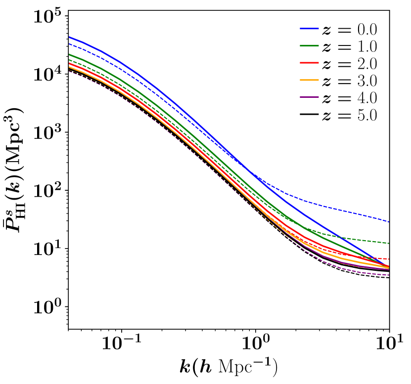
Figure 3: Power spectrum monopole of HI including (solid thick lines) and without (dashed thin lines) the effect of RSD, modelled by Eq. 29.

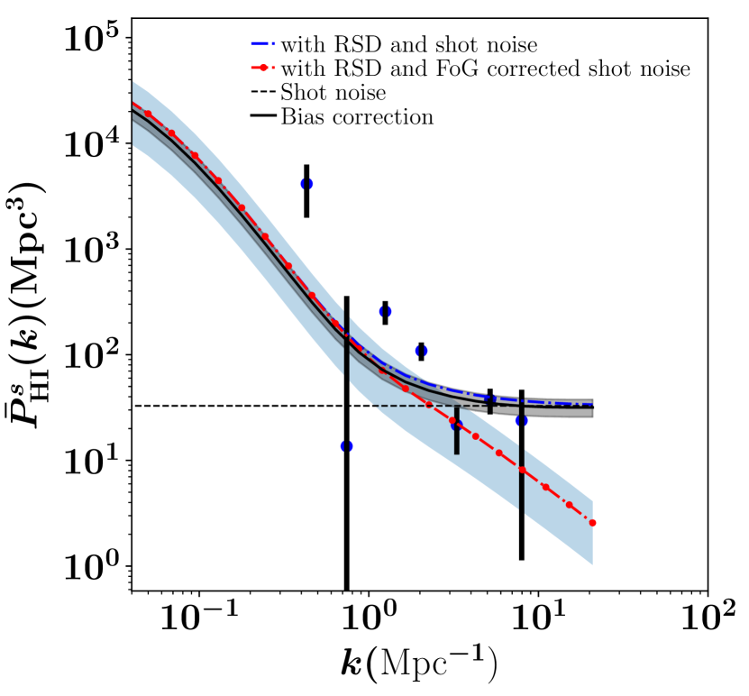
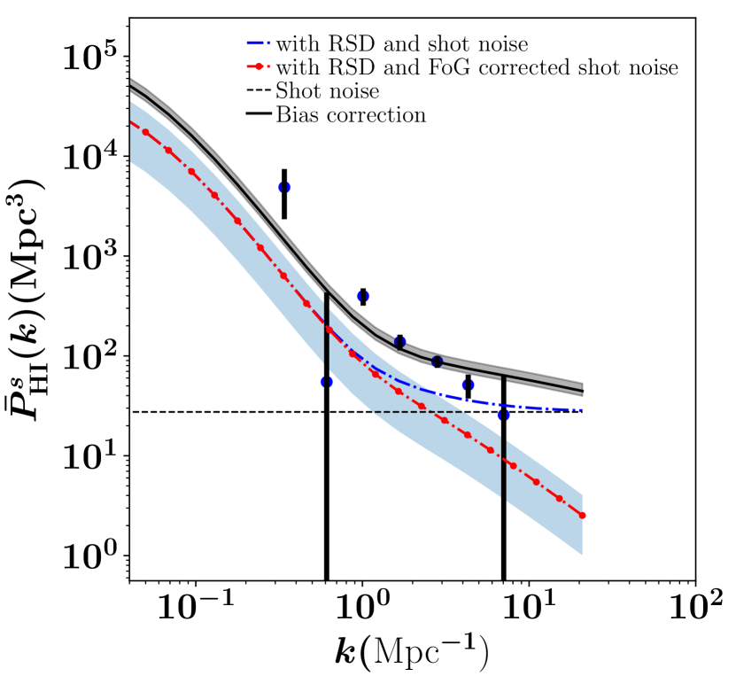
Figure 4: Power spectrum in the halo-model framework, using the 1- and 2-halo terms with RSD and shot noise incorporating the Gaussian finger-of-god corrections (dot-dashed blue and red lines), compared to the MeerKAT intensity mapping results (dark blue points with error bars) at $z=0.32$ (top panel) and $z=0.44$ (lower panel). The expected scatter due to astrophysical uncertainties (Padmanabhan, 2021) is shown by the blue shaded band. The best-fitting curve to the data, leaving free a scaling to the amplitude of the power spectrum, is shown by the black solid line, with the associated uncertainty in the inferred amplitude parameter indicated by the grey band.

We now illustrate the comparison of these findings to the recent MeerKAT intensity mapping observations in Fig. 4. The intensity mapping power spectra cover two redshift bins centred at $z=0.32$ and $z=0.44$ respectively (with the HI mass function at $z\sim 0.32$ presented in the previous section having been derived from the corresponding power spectrum). The solid green lines in Fig. 4 show the power spectrum including only the 1- and 2-halo terms, in which only the 1-halo term contributes to the small scales. Overplotted are the dashed-dotted blue lines that show the effect of adding the shot noise Eq. 24 and the exponential finger-of-god suppression described above. The shot noise term for an intensity mapping experiment may be modulated by the finger-of-god terms since the point sources are expected to be smeared out (Paul et al., 2023). This leads to

$$P_{\rm SN}^{\rm fog}(k)=\frac{1}{\bar{\rho}_{\rm HI}^{2}}\!\int\mbox{d}M\,n(M)M_{\rm HI}^{2}\,\mathcal{R}_{3}(k\sigma)\;,$$ (34)

where the integrand in Eq. 24 has been modified by the damping term

$$\mathcal{R}_{3}(y)=\frac{\sqrt{\pi}}{2}\frac{{\rm erf}(y)}{y}.$$ (35)

The power spectrum with the above correction to the shot noise is also plotted in Fig. 4 as the red dot-dashed lines.

The dark blue data points with error bars show the MeerKAT measurements. They are in line with the halo model predictions at $z=0.32$, including shot noise and RSD. This is also borne out by the fact that a best-fit to the data, leaving free a scaling to the amplitude of the power spectrum, does not lead to significantly different results. Specifically, we apply such a bias correction only to the non-RSD corrected portion of the power spectrum:

$$P_{\rm corr}(k)=A_{b}^{2}{\bar{P}}_{\rm HI}(k)+\big{[}{\bar{P}}^{\rm s}_{\rm HI}(k)-{\bar{P}}_{\rm HI}(k)\big{]}+P_{\rm SN}\,.$$ (36)

We find that the best-fitting value of $A_{b}=0.89\pm 0.20$, as enclosed by the solid black curve, with the uncertainty in $A_{b}$ covered by the grey shaded region. This shows that the amplitude hike is consistent with unity.

At $z=0.44$, however, the data favour a greater amplitude of the power than predicted by the theory alone, which could have different possible causes. The above procedure results in a best-fitting value $A_{b}=1.62\pm 0.10$, as shown by the black solid line and grey shaded region in that figure (note that the grey shading only shows the uncertainty in the fitting of the $A_{b}$ parameter). This value captures a possible remaining correction to the power which may result from higher-order biases not related only to the DM power as well as yet-unknown baryonic or other factors. The overall uncertainty in the fitting could be represented by the combined effect of the blue and grey shaded regions.

5 Discussion

We have examined the effects that modify the power spectrum of HI on small scales, using the latest results from the MeerKAT intensity mapping experiment to constrain the free parameters. In so doing, we have developed analytical fitting forms for the small scale structure of the HI intensity power spectra arising from the halo model framework. We have additionally included the contributions of shot noise, with and without a finger-of-god damping.

The behaviour of the HI mass - halo mass relation is consistent with the expectations of the halo model framework and also matches the findings of recent HI galaxy surveys in the relevant mass range (Bera et al., 2022). The measured power spectrum at $z=0.32$ is consistent with the expectations from the halo model, as also borne out by fitting the data directly leaving free an overall scaling to the amplitude of the power spectrum. Such a procedure at $z=0.44$ may indicate some evidence for a higher than expected amplitude corresponding to a constant increase to the HI bias that we obtained in the halo-model framework. This could have different possible causes, including higher-order biases not related to dark matter as suggested in SPT/EFT models. Beyond-EFT effects, such as the fact that the velocities of HI and dark matter do not agree on small scales and various complex baryonic effects may also contribute. The fitting procedure also indicates evidence favouring the standard shot noise term from Eq. 24 at small scales (rather than its finger-of-god modulated version Eq. 34).

An additional consideration is the presence of nonzero vorticity in the dark matter, which adds a correction to the HI power spectrum. This correction is found via N-body simulations and can be modelled as (Cusin et al., 2017):

$$P_{{\rm m},\omega}(k,z=0)=\frac{k^{2}}{2\pi^{3}}\frac{A_{\omega}\,(k/k_{*})^{n_{l}}}{\big{[}1+(k/k_{*})\big{]}^{n_{l}+n_{s}}}\,(\rm Mpc/h)^{3}\;.$$ (37)

Typical values of the parameters $k_{*},n_{l}$ and $n_{s}$ produce a peak in vorticity power at $k\sim 1\,h/$Mpc. The amplitude parameter $A_{\omega}$ is more uncertain. Most simulations find $A_{\omega}\sim 10^{-5}$, with some advocating a value 50-100 times larger (Bonvin et al., 2018; Pueblas & Scoccimarro, 2009). These values are found to be too low to explain the observed difference in the predicted and measured HI power in the current data. However, a more detailed treatment of the effects of vorticity is left to future work (Umeh et al., in preparation).

At $z\sim 0.3$, the parameter $\Omega_{\rm HI}$ has been measured to be $4.8\times 10^{-4}$ also from surveys of galaxies (Bera et al., 2019), which is consistent with the value we use here, though as also suggested by the intensity mapping results, there may be evidence for an evolution with respect to mass (Bera et al., 2022). At $z\sim 0.4$, the HI mass has been connected to the stellar mass of MeerKAT MIGHTEE galaxies, finding some evolution in the relationship out to $z\sim 1$.

Future data sets would be useful to consolidate these findings to develop an deeper understanding of the role of HI in the baryon cycle for $z\sim 0$–$1$. The above formalism holds for any tracer of the dark matter which is in a mass-dependent form, so it would be equally applicable to small-scale effects in surveys probing CO/[CII]/[OIII] lines in the microwave and submillimetre regimes (GHz and THz frequencies, for reviews see, e.g., Bernal & Kovetz, 2022; Kovetz et al., 2019). Thus far, the single-dish surveys used for measuring intensity fluctuations of these tracers lead to a suppression of the power spectrum on scales smaller than the beam size (e.g. Padmanabhan et al., 2022), which is where most of the effects considered here become relevant. This may, however, become possible with the availability of surveys probing smaller scales in other tracers in the future.

Appendix A The two-dimensional power spectrum

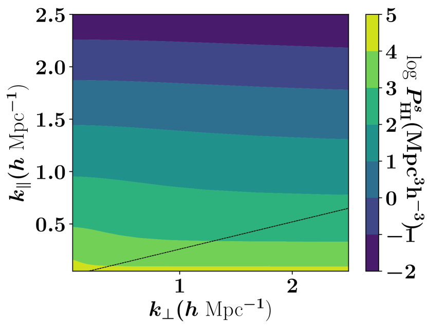
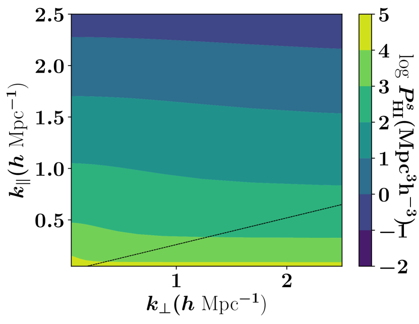
Figure 5: Two dimensional power spectra in redshift space with the parameters following the halo model prescription of Padmanabhan et al. (2017) and the Gaussian finger-of-god effects as discussed in the main text, at $z=0.32$ (top) and $z=0.44$ (lower panel). The conservative horizon limit for the MeerKAT results is shown in each figure by the black dotted line.

The two-dimensional power spectrum, i.e. in the $(k_{\perp},k_{\parallel})$ plane, contains more information than the monopole of the power spectrum considered in Section 4:

$$P_{\rm HI}^{\rm s}(k_{\parallel},k_{\perp})=P_{\rm HI}({k_{\parallel},k_{\perp}})\bigg{(}1+\frac{k_{\parallel}^{2}}{k_{\parallel}^{2}+k_{\perp}^{2}}\,\frac{f}{b_{\rm HI}}\bigg{)}^{2}\exp\big{(}{-{k_{\parallel}^{2}}\sigma_{\rm avg}^{2}}\big{)}.$$ (38)

The resultant 2D power spectra are displayed in Fig. 5, for the two redshifts, $z=0.32,\,0.44$.

The horizon limit of the MeerKAT interferometer, below which foregrounds are expected to become relevant, is defined through (e.g. Liu et al., 2014):

$$k_{\parallel}=\frac{r(z){H}(z)\sin\theta_{0}}{c(1+z)}\,k_{\perp}{\simeq 0.02\,k_{\perp}}\,.$$ (39)

Here $r$ is the comoving radial distance and $\theta_{0}$ is a characteristic of the beam (Paul et al., 2023). The horizon adopted in the analysis of Paul et al. (2023) is conservatively taken to be about 10 times stricter, $k_{\parallel}=0.26k_{\perp}$. This is shown by the black dotted lines in Fig. 5.

References

- Anderson et al. (2018) Anderson C. J., et al., 2018, MNRAS, 476, 3382
- Bera et al. (2019) Bera A., Kanekar N., Chengalur J. N., Bagla J. S., 2019, ApJ, 882, L7
- Bera et al. (2022) Bera A., Kanekar N., Chengalur J. N., Bagla J. S., 2022, ApJ, 940, L10
- Bernal & Kovetz (2022) Bernal J. L., Kovetz E. D., 2022, arXiv e-prints, p. arXiv:2206.15377
- Bonvin et al. (2018) Bonvin C., Durrer R., Khosravi N., Kunz M., Sawicki I., 2018, J. Cosmology Astropart. Phys., 2018, 028
- Chang et al. (2010) Chang T.-C., Pen U.-L., Bandura K., Peterson J. B., 2010, arXiv e-prints, p. arXiv:1007.3709
- Chowdhury et al. (2021) Chowdhury A., Kanekar N., Das B., Dwarakanath K. S., Sethi S., 2021, ApJ, 913, L24
- Chowdhury et al. (2022) Chowdhury A., Kanekar N., Chengalur J. N., 2022, ApJ, 941, L6
- Cooray & Sheth (2002) Cooray A., Sheth R., 2002, Phys. Rep., 372, 1
- Cunnington et al. (2023) Cunnington S., et al., 2023, MNRAS, 518, 6262
- Cusin et al. (2017) Cusin G., Tansella V., Durrer R., 2017, Phys. Rev. D, 95, 063527
- Kaiser (1987) Kaiser N., 1987, MNRAS, 227, 1
- Kovetz et al. (2019) Kovetz E., et al., 2019, BAAS, 51, 101
- Liu et al. (2014) Liu A., Parsons A. R., Trott C. M., 2014, Phys. Rev. D, 90, 023018
- Macciò et al. (2007) Macciò A. V., Dutton A. A., van den Bosch F. C., Moore B., Potter D., Stadel J., 2007, MNRAS, 378, 55
- Masui et al. (2013) Masui K. W., et al., 2013, ApJ, 763, L20
- Padmanabhan (2021) Padmanabhan H., 2021, International Journal of Modern Physics D, 30, 2130009
- Padmanabhan & Kulkarni (2017) Padmanabhan H., Kulkarni G., 2017, MNRAS, 470, 340
- Padmanabhan & Refregier (2017) Padmanabhan H., Refregier A., 2017, MNRAS, 464, 4008
- Padmanabhan et al. (2017) Padmanabhan H., Refregier A., Amara A., 2017, MNRAS, 469, 2323
- Padmanabhan et al. (2022) Padmanabhan H., Breysse P., Lidz A., Switzer E. R., 2022, MNRAS, 515, 5813
- Paul et al. (2023) Paul S., Santos M. G., Chen Z., Wolz L., 2023, arXiv e-prints, p. arXiv:2301.11943
- Peacock & Dodds (1994) Peacock J. A., Dodds S. J., 1994, MNRAS, 267, 1020
- Pueblas & Scoccimarro (2009) Pueblas S., Scoccimarro R., 2009, Phys. Rev. D, 80, 043504
- Sarkar & Bharadwaj (2018) Sarkar D., Bharadwaj S., 2018, MNRAS, 476, 96
- Seehars et al. (2016) Seehars S., Paranjape A., Witzemann A., Refregier A., Amara A., Akeret J., 2016, J. Cosmology Astropart. Phys., 2016, 001
- Seljak (2000) Seljak U., 2000, MNRAS, 318, 203
- Seo et al. (2010) Seo H.-J., Dodelson S., Marriner J., Mcginnis D., Stebbins A., Stoughton C., Vallinotto A., 2010, ApJ, 721, 164
- Sinigaglia et al. (2022) Sinigaglia F., et al., 2022, ApJ, 935, L13
- Switzer et al. (2013) Switzer E. R., et al., 2013, MNRAS, 434, L46
- Villaescusa-Navarro et al. (2018) Villaescusa-Navarro F., et al., 2018, ApJ, 866, 135
- White (2001) White M., 2001, MNRAS, 321, 1
- Wolz et al. (2022) Wolz L., et al., 2022, MNRAS, 510, 3495
- Zhang et al. (2020) Zhang J., Costa A. A., Wang B., He J.-h., Luo Y., Yang X., 2020, ApJ, 895, 34