Composite Dark Matter and Neutrino Masses from a Light Hidden Sector

Abstract

We study a class of models in which the particle that constitutes dark matter arises as a composite state of a strongly coupled hidden sector. The hidden sector interacts with the Standard Model through the neutrino portal, allowing the relic abundance of dark matter to be set by annihilation into final states containing neutrinos. The coupling to the hidden sector also leads to the generation of neutrino masses through the inverse seesaw mechanism, with composite hidden sector states playing the role of the singlet neutrinos. We focus on the scenario in which the hidden sector is conformal in the ultraviolet, and the compositeness scale lies at or below the weak scale. We construct a holographic realization of this framework based on the Randall-Sundrum setup and explore the implications for experiments. We determine the current constraints on this scenario from direct and indirect detection, lepton flavor violation and collider experiments and explore the reach of future searches. We show that in the near future, direct detection experiments and searches for $\mu\rightarrow e$ conversion will be able to probe new parameter space. At colliders, dark matter can be produced in association with composite singlet neutrinos via Drell Yan processes or in weak decays of hadrons. We show that current searches at the Large Hadron Collider have only limited sensitivity to this new production channel and we comment on how the reconstruction of the singlet neutrinos can potentially expand the reach.

1 Introduction

Despite the remarkable success of the Standard Model (SM) in explaining the interactions of the elementary particles, there is now indisputable evidence that it is incomplete. In particular, cosmological and astrophysical observations have established that more than 80% of the matter in the universe is composed of some form of non-luminous, cold dark matter (DM), but there is no particle in the SM that can play this role. Furthermore, although the SM predicts that the neutrinos are massless, over the last few decades various oscillation experiments have established that the masses of the neutrinos, although tiny relative to those of the other SM fermions, are non-vanishing. Any explanation of these puzzles require new physics beyond the SM.

At present, the nature of the particles of which DM is composed remains completely unknown. One interesting possibility is that the particles that constitute DM are the composites of a strongly coupled hidden sector. Within this class of theories, the DM candidates that have been studied include dark glueballs [1, 2], dark pions [3, 4, 5, 6, 7] and dark baryons [8, 9, 10]. For a clear review of composite DM with many additional references, see [11]. Another intriguing possibility is that there is a close connection between the particles that constitute DM and the SM neutrinos. Examples of such theories include sneutrino DM in supersymmetric extensions of the SM [12, 13, 14], sterile neutrino DM [15, 16, 17], and scotogenic models of neutrino masses [18, 19, 20].

In this paper, we propose a new class of composite DM models that can account for both the observed abundance of DM and the origin of neutrino masses. We consider a scenario in which the particle that constitutes the observed DM arises as a composite state of a strongly coupled hidden sector. The stability of DM is ensured by a discrete symmetry of the hidden sector. The SM is assumed to couple to the hidden sector through the neutrino portal.  This allows the relic abundance of DM to be set by annihilation to a final state consisting of a SM neutrino and antineutrino, or alternatively, to a final state consisting of a SM (anti)neutrino and a composite hidden sector particle. The neutrino portal interaction leads to mixing of the SM neutrinos with composite fermions of the hidden sector. The neutrinos thereby acquire tiny Majorana masses through the inverse seesaw mechanism [24, 25]. In this framework, the neutrinos are partially composite.  We focus on a scenario in which the compositeness scale lies below the weak scale, leading to rich experimental signals.

The strong dynamics of the hidden sector is taken to be approximately conformal in the ultraviolet. This can allow the small parameters necessary to explain the observed neutrino masses within the framework of a low-scale seesaw model to naturally arise from the scaling dimensions of operators in the conformal field theory (CFT) [35]. To explore the dynamics of this class of models, we construct a holographic realization of this scenario based on the AdS/CFT correspondence [36, 37, 38, 39]. The correspondence relates large-$\mathcal{N}$ CFTs in four dimensions to theories of gravity in warped space in a higher number of dimensions. Our realization takes the form of a five-dimensional (5D) Randall-Sundrum (RS) model with two branes [40]. Operators in the hidden sector CFT are dual to fields in the bulk whereas the SM fields, being elementary, are mapped to states localized on the ultraviolet brane. Within this framework, we can calculate the relic abundance of DM and explore the phenomenology associated with this class of models.

Within the framework of the RS solution to the hierarchy problem, several authors have addressed the generation of neutrino masses, for example, [41, 42, 43, 44, 45], and the origin of DM, for example, [46, 47, 48, 49]. However, an important difference is that because these models are built around the RS solution to the hierarchy problem, all the SM quarks and leptons are necessarily partially or entirely composite. The compositeness scale is then constrained to lie above a TeV, and so the implications for experiments are very different. A holographic model of neutrino masses with a lower compositeness scale that shares some features with our construction was considered in [50] (see also [51]).

This class of DM models gives rise to signals in direct and indirect detection experiments and at colliders. Since the couplings of the hidden sector to the SM through the neutrino portal will in general violate flavor, we also expect signals in experiments searching for lepton flavor violating processes, such as $\mu\rightarrow e\gamma$ and $\mu\rightarrow e$ conversion. We determine the constraints from existing searches and explore the reach of future experiments. In this framework, although the hidden sector is neutral under the weak interactions, the DM acquires a coupling to the $Z$-boson at loop level through the neutrino portal interaction and can therefore be searched for in direct detection experiments. We find that for some range of DM masses, future direct detection experiments such as LZ [52] and XENONnT [53] will have sensitivity to this scenario. In some regions of parameter space, in addition to neutrinos, other SM particles are also produced as the result of DM annihilation. This can be used to constrain the model in indirect detection experiments, both from precision observations of the CMB and from searches for gamma rays and positrons that are the products of DM annihilation.

The spectrum of composite states includes singlet neutrinos that carry a small charge under the weak interactions through their mixing with the SM neutrinos. These particles fall into the category of heavy neutral leptons (HNLs), which are being searched for at the LHC and at beam dumps. However, the composite singlet neutrinos differ from conventional HNLs in that, in some regions of parameter space, their primary decay mode is completely invisible. For the case when the dominant decays of the composite singlet neutrinos are visible, we use the current limits on HNLs to place bounds on this scenario and study the reach of future searches. Since the hidden sector couples to the SM through the neutrino portal, DM particles can also be produced in association with a composite singlet neutrino. The challenge in detecting DM is therefore to identify the effects of additional invisible particles on top of standard HNL signatures. We study the sensitivity of existing experimental HNL searches for events produced via this new channel, and we also explore a strategy involving the reconstruction of the HNL that would extend the reach for DM particles. We find that, although the parameter space of the model is highly constrained by non-collider observations, there is nevertheless a limited region where these searches have sensitivity.

The outline of the paper is as follows. We discuss the general framework in Sec. 2. In Sec. 3, we lay out the extra-dimensional model and determine the mass spectra, couplings and mixing angles. In Sec. 4, we present a comprehensive phenomenological analysis of DM with a focus on its production, direct and indirect detection. The collider aspects of the phenomenology are presented in Sec. 5. We conclude in Sec. 6.

2 A Framework for Composite Dark Matter and Neutrino Masses

In this section, we outline the general features of the scenario we are exploring. We consider a framework in which the particle that constitutes DM arises as a composite state of a strongly coupled hidden sector that is approximately conformal in the ultraviolet. We show that couplings between the hidden sector and the SM through the neutrino portal can give rise to the observed abundance of DM, while also generating the neutrino masses. We discuss the current constraints on this class of models and outline the possibilities for discovering the DM candidate in direct and indirect detection experiments and collider searches.

2.1 Composite Dark Metter through the Neutrino Portal

Consider a hidden sector composed of a strongly coupled CFT, to which we add a relevant deformation ${\cal O}_{\rm def}$,

$${\cal L}_{\rm UV}\supset{\cal L}_{\rm CFT}+\lambda_{\rm def}{\cal O}_{\rm def}\;.$$ (2.1)

When the deformation grows large in the infrared (IR), it causes the breaking of the conformal dynamics. This occurs at a scale that we denote by $\Lambda$.

We assume that the spectrum of light hidden sector states includes three composite Dirac fermions $N^{\alpha}$, which play the role of composite singlet neutrinos. Here $\alpha=1,2,3$ represents a flavor index. The low energy effective Lagrangian contains kinetic and mass terms for the singlet neutrinos,

$${\cal L}_{\rm IR} \supset i\bar{N}\gamma^{\mu}\partial_{\mu}N-m_{N}\bar{N}N,$$ (2.2)

where we have suppressed the flavor indices. Here $m_{N}$ is the singlet neutrino mass, which is expected to be of the order of the conformal symmetry breaking scale $\Lambda$. We can decompose $N$ into components with left- and right-handed chiralities, $N=(N_{L},N_{R})$.

The hidden sector interacts with the SM through the neutrino portal,

$${\cal L}_{\rm UV}\supset-\frac{\hat{\lambda}}{M_{\mathrm{UV}}^{\Delta_{\widehat{N}}-3/2}}\bar{L}\widetilde{H}\mathcal{\widehat{O}}_{\!N}+\mathrm{h.c.},$$ (2.3)

where $L$ is the SM left-handed lepton doublet, $\widetilde{H}\equiv i\sigma_{2}H^{\ast}$ where $H$ is the SM Higgs doublet, and $\mathcal{\widehat{O}}_{\!N}$ represents a primary operator of scaling dimension $\Delta_{\widehat{N}}$ that transforms as a right-handed Weyl fermion. Here $\hat{\lambda}$ is a dimensionless coupling constant and $M_{\rm UV}$ denotes the ultraviolet (UV) cutoff of the theory. At the conformal breaking scale $\Lambda$, this interaction gives rise to the following term in the low-energy Lagrangian,

$${\cal L}_{\rm IR} \supset-\lambda\,\bar{L}\widetilde{H}N_{\!R}+{\rm h.c.},$$ (2.4)

where the dimensionless coupling $\lambda$ scales as

$$\lambda\sim\hat{\lambda}\left(\frac{\Lambda}{M_{\mathrm{UV}}}\right)^{\Delta_{\widehat{N}}-3/2}.$$ (2.5)

This represents a coupling of the SM to the composite singlet neutrinos $N_{\!R}$ through the neutrino portal. Once Higgs acquires a vacuum expectation value (VEV), this interaction and the mass term in Eq. (2.6) lead to mixing between the SM neutrinos and the composite fermions $N_{\!L}$. Therefore the light neutrinos contain an admixture of hidden sector states, while the composite singlet neutrinos acquire an admixture of the SM neutrino. In this way the composite singlet neutrinos acquire a small coupling to the weak gauge bosons of the SM.

The scaling dimension of the primary fermionic operator $\mathcal{\widehat{O}}_{\!N}$ is bounded from below by unitarity, $\Delta_{\widehat{N}}\geq 3/2$, where the limiting case of $\Delta_{\widehat{N}}=3/2$ corresponds to the case of a free fermion. On the other hand, for scaling dimensions $\Delta_{\widehat{N}}\geq 5/2$ the interaction in Eq. (2.3) leads to the theory becoming ultraviolet sensitive, which requires the addition of new counterterms involving the SM fields for consistency [35]. Therefore, in this work, we limit our analysis to values of the scaling dimension of $\mathcal{\widehat{O}}_{\!N}$ in the range $3/2<\Delta_{\widehat{N}}<5/2$. With this choice of $\Delta_{\widehat{N}}$, the coupling $\lambda$ in Eq. (2.5) is hierarchically small for $\Lambda\ll M_{\rm UV}$, so that the mixing between the SM neutrinos and their singlet counterparts is suppressed. As we explain below, this feature of our model can help explain both the smallness of the neutrino masses and the observed abundance of DM. In this work, we focus on low values of the compositeness scale, corresponding to values of $\Lambda$ at or below the electroweak scale.

We now assume that at the scale $\Lambda$, in addition to the composite singlet neutrinos $N$, the spectrum of hidden sector states also includes a composite Dirac fermion $\chi$, which plays the role of DM. Then the low energy Lagrangian at scales of order $\Lambda$ includes the terms,

$${\cal L}_{\rm IR}\supset \,i\bar{\chi}\gamma^{\mu}\partial_{\mu}\chi-m_{\chi}\bar{\chi}\chi\;.$$ (2.6)

Here $m_{\chi}$ is the DM mass, which we again take to be of the order of $\Lambda$. To ensure the stability of DM we assume that the hidden sector respects a discrete $Z_{2}$ symmetry under which $\chi$ is odd, but the singlet neutrinos $N$ as well as the SM fields are even. We further assume that there are no Nambu-Goldstone bosons or other light states, so $\chi$ is the lightest state in the hidden sector.

In our framework, the neutrino portal interaction keeps the hidden sector in equilibrium with the SM in the early universe. Because of the composite nature of the fermions $\chi$ and $N$, the low energy theory at the scale $\Lambda$ contains nonrenormalizable interactions between the DM particle and the singlet neutrinos of the schematic form,

$${\cal L}_{\rm IR} \supset-\frac{\tilde{\kappa}}{\Lambda^{2}}(\bar{\chi}N)(\bar{N}\chi)\;,$$ (2.7)

where $\tilde{\kappa}$ is of order $16\pi^{2}/\mathcal{N}^{2}$ in the large-$\mathcal{N}$ limit. Once the temperature falls below $m_{\chi}$, these interactions allow the DM particles to annihilate away through processes such as $\chi\bar{\chi}\rightarrow(\nu\bar{N},N\bar{\nu})$ and $\chi\bar{\chi}\rightarrow\nu\bar{\nu}$. Naively, the annihilation rate would be expected to be enhanced compared to the freeze-out of DM of weak scale mass because of the low scale $\Lambda$ that sets the mass of $\chi$ and the strength of its interactions, resulting in a too low abundance of DM. However, this can be compensated for by the small mixing between the SM neutrinos and the composite singlet neutrinos. This class of theories can therefore easily accommodate the observed abundance of DM.

2.2 Neutrino masses via the Inverse Seesaw Mechanism

In this subsection, we outline how this framework can naturally incorporate the generation of neutrino masses through the inverse seesaw mechanism. Our discussion is based on the analysis in [35]. We now assume that the hidden sector possesses a global symmetry under which the operator $\mathcal{\widehat{O}}_{\!N}$ is charged. The charges under this global symmetry can be normalized such that $\mathcal{\widehat{O}}_{\!N}$, and therefore $N_{\!R}$, carries charge $+1$. Then, we see from the coupling Eq. (2.4) that this symmetry can be subsumed into an overall lepton number symmetry under which both $N_{\!R}$ and $N_{\!L}$ carry charge $+1$.

In order to employ the inverse seesaw mechanism to generate the SM neutrino masses, we require a source of lepton number violation in the model. Accordingly, we add to the theory a lepton number violating deformation arising from an operator ${\cal O}_{2N}$, which has scaling dimension $\Delta_{2N}$,

$$\mathcal{L}_{\rm UV}\supset-\frac{\hat{\mu}}{M_{\mathrm{UV}}^{\Delta_{2N}-4}}{\cal O}_{2N}+\mathrm{h.c.}$$ (2.8)

Here $\hat{\mu}$ is a dimensionless constant that parametrizes the strength of the deformation. We assume that ${\cal O}_{2N}$ carries a charge of $+2$ under the global symmetry of the hidden sector, so that this deformation violates lepton number by two units. In the low-energy effective theory at the scale $\Lambda$, this gives rise to terms in the Lagrangian of the form,

$${\cal L}_{\rm IR} \supset-(\mu N_{\!L}N_{\!L}+\mu^{\prime}N_{\!R}N_{\!R})+\textrm{h.c.}\,,$$ (2.9)

where the Majorana masses $\mu$ and $\mu^{\prime}$ parameterize the strength of lepton number violation. Their values scale with the parameters of the theory as

$$\mu\sim\mu^{\prime}\sim\hat{\mu}\Lambda\left(\frac{\Lambda}{M_{\mathrm{UV}}}\right)^{\Delta_{2N}-4}.$$ (2.10)

The scaling dimension $\Delta_{2N}$ of the lepton number violating scalar operator ${\cal O}_{2N}$ is constrained by unitarity to satisfy $\Delta_{2N}\geq 1$, where the limiting case $\Delta_{2N}=1$ corresponds to the case of a free scalar. For $\Delta_{2N}>4$, the Majorana mass terms $\mu$ and $\mu^{\prime}$ are hierarchically smaller than $\Lambda$.

With the inclusion of the lepton number violating terms in Eq. (2.9) the low-energy effective theory now possesses all the ingredients required to realize inverse seesaw mechanism,

$${\cal L}_{\rm IR}\supset i\bar{N}\gamma^{\mu}\partial_{\mu}N-m_{N}\bar{N}N-\Big{[}\mu N_{\!L}N_{\!L}+\lambda\bar{L}\widetilde{H}N_{\!R}+{\rm h.c.}\Big{]}.$$ (2.11)

By integrating out the composite singlet neutrinos $N$ we obtain a contribution to the masses of the light neutrinos,

$$m_{\nu}=\mu\Big{(}\frac{\lambda v_{\rm EW}}{m_{N}}\Big{)}^{2}\;.$$ (2.12)

Here $v_{\rm EW}\equiv\langle H\rangle\simeq 174\;\hbox{GeV}$. When the effects of higher resonances are included, this relation is only approximate, so that

$$m_{\nu}\sim\mu\Big{(}\frac{\lambda v_{\rm EW}}{m_{N}}\Big{)}^{2}\;.$$ (2.13)

Note that the neutrino masses depend on both the parameter $\lambda$, which controls the mixing with the composite states as seen in Eq. (2.5), and the parameter $\mu$, which controls the extent of lepton number violation as seen in Eq. (2.10). Then the smallness of the SM neutrino masses can naturally be explained by either the small parameter $\lambda$ that sets the size of the neutrino mixing or the small lepton number violating coupling $\mu$. Since the small values of these parameters admit a simple explanation in terms of the scaling dimensions of the operators $\mathcal{\widehat{O}}_{\!N}$ and ${\cal O}_{2N}$, this class of models can provide a natural explanation for the smallness of neutrino masses.

Note that in this construction both the Dirac mass term $\lambda v_{\rm EW}$ and the Majorana mass term $\mu$ need to be smaller than the compositeness scale $\Lambda$. This leads to the following range for the coupling $\lambda$,

$$\frac{\sqrt{m_{\nu}m_{N}}}{{v_{\rm EW}}} \lesssim\lambda\lesssim\frac{m_{N}}{v_{\rm EW}}\;,$$ (2.14)

where we have employed Eq. (2.13) in obtaining the lower bound, after setting $m_{N}\sim\Lambda$.

The neutrino mixing angle to the physical mass eigenstates in the limit $m_{N}\gg\lambda v_{\rm EW}$ is defined as,

$$U_{N\ell}\equiv\frac{\lambda v_{\rm EW}}{m_{N}}.$$ (2.15)

It follows from Eqs. (2.14) and (2.15) that the mixing angle $U_{N\ell}$ lies in the range

$$\sqrt{\frac{m_{\nu}}{m_{N}}} \lesssim U_{N\ell}\lesssim 1\;.$$ (2.16)

2.3 Abundance of Dark Matter

In this subsection, we outline how this class of models can reproduce the observed abundance of DM. At high temperatures in the early universe, the hidden sector was in thermal contact with SM through the portal operator in Eq. (2.3). This interaction populates the hidden sector, bringing it into thermal equilibrium with the SM. Once the temperature falls below their masses, the hidden sector states begin to exit the bath. The observed DM today is composed of the lightest $Z_{2}$ odd Dirac fermion $\chi$ that survives as a thermal relic.

We first show that the hidden sector is in thermal equilibrium with the SM at temperatures of order the compositeness scale. The hidden sector states can be produced from SM neutrinos via processes such as $\nu\nu\to{\cal U}_{N}$, $\nu\nu\to\nu{\cal U}_{N}$, $\nu{\cal U}_{N}\to\nu{\cal U}_{N}$, where the label ${\cal U}_{N}$ denotes hidden sector states. To see this, note that the strongly coupled nature of the hidden sector implies large self-interactions between the composite singlet neutrino states,

$$\mathcal{L}_{\mathrm{IR}}\supset-\frac{\kappa}{\Lambda^{2}}\left(\bar{N}\gamma^{\mu}N\right)^{2}+\cdots,$$ (2.17)

where the size of the coupling $\kappa$ is of the order of $\sim(4\pi)^{2}/\mathcal{N}^{2}$ in the large-$\mathcal{N}$ limit and the ellipses denote other Lorentz contractions. These interactions are characteristic of the composite nature of the singlet neutrinos. To see that the hidden sector is in equilibrium with the SM at temperatures $T$ of order $\Lambda$, we estimate the rate for the $\nu\nu\to{\cal U}_{N}$ process. When $T\sim\Lambda$, this rate is expected to be parametrically of the same order as the $\nu\nu\to NN$ rate. From Eq. (2.17) we can estimate the cross section for this process as,

$$\sigma_{\nu\nu\rightarrow\mathcal{U}_{N}}\sim\sigma_{\nu\nu\rightarrow NN}\sim\frac{1}{4\pi}\bigg{(}\frac{\kappa}{\Lambda^{2}}\bigg{)}^{2}\big{|}U_{N\ell}\big{|}^{4}\,T^{2}.$$ (2.18)

From this, we can write the thermally averaged interaction rate as,

$$\bar{n}_{\nu}\langle\sigma_{\nu\nu\to NN}\,v\rangle\sim\frac{\kappa^{2}}{4\pi}\big{|}U_{N\ell}\big{|}^{4}\,\frac{T^{5}}{\Lambda^{4}}\,,$$ (2.19)

where $\bar{n}_{\nu}\sim T^{3}$ represents the equilibrium number density of SM neutrinos. In order to keep the SM and hidden sector in thermal and chemical equilibrium at the compositeness scale the above interaction rate should be larger than the Hubble rate $H\sim T^{2}/M_{\rm Pl}$ at temperature $T\sim\Lambda$, where $M_{\rm Pl}$ denotes the Planck mass. Taking $\kappa\sim(4\pi)^{2}$, the condition for thermal equilibrium condition at temperature $T\sim\Lambda$ can be translated into a lower bound on the neutrino mixing angle $U_{N\ell}$ as,

$$|U_{N\ell}|^{2}\gtrsim\sqrt{\Lambda/4\pi M_{\rm Pl}}\,.$$ (2.20)

As we shall see, this result means that the SM and the hidden sector will be in equilibrium at early times for the range of mixing angles that leads to the observed abundance of DM after thermal freeze-out.

In our framework the abundance of DM is set by the standard thermal freeze-out mechanism. As the temperature falls below the compositeness scale, DM annihilates to the visible sector through the neutrino portal and eventually freezes out as a thermal relic. The dominant DM annihilation channels to the visible sector are,

$$\hskip 28.45274pt\chi\bar{\chi}\to\left(N\bar{\nu},\nu\bar{N}\right)\hskip 28.45274pt\chi\bar{\chi}\to\nu\bar{\nu}.$$ (2.21)

The Feynman diagrams for the above DM annihilation processes are shown in Fig. 1, where the vertex shown as a red-square corresponds to the interaction between DM and singlet neutrinos given in Eq. (2.7) and a blue-circle denotes the neutrino mixing angle $U_{N\ell}$.

Figure 1: Feynman diagrams for DM annihilation are shown above where the composite DM–neutrino effective vertex $\kappa/\Lambda^{2}$ is denoted by a red-square and neutrino mixing $U_{N\ell}$ is shown as a blue circle. For the left diagram, there is an analogous process for the final state $\bar{N}\nu$. Flavor indices on the neutrinos have been suppressed.

The cross sections for the above DM annihilation processes at temperatures $T$ of order $\Lambda$ can be estimated as,

$$\sigma_{\chi\bar{\chi}\to N\bar{\nu}}\sim\frac{\tilde{\kappa}^{2}\,U_{N\ell}^{2}}{4\pi}\frac{T^{2}}{\Lambda^{4}},\hskip 28.45274pt\sigma_{\chi\bar{\chi}\to\nu\bar{\nu}}\sim\frac{\tilde{\kappa}^{2}\,U_{N\ell}^{4}}{4\pi}\frac{T^{2}}{\Lambda^{4}}.$$ (2.22)

DM freeze-out happens when its thermally averaged interaction rate becomes comparable to the Hubble rate, $\bar{n}_{\chi}\langle\sigma v\rangle\sim H\sim T^{2}/M_{\rm Pl}$, where $\bar{n}_{\chi}\sim(m_{\chi}T)^{3/2}\,e^{-m_{\chi}/T}$ is the non-relativistic equilibrium number density for DM. The freeze-out happens at temperatures $T$ of order $m_{\chi}/10$.

The thermally averaged DM annihilation cross sections at DM freeze-out, i.e. for $T=T_{\rm fo}\sim m_{\chi}/10$, can be estimated as,

$$\langle\sigma_{\chi\bar{\chi}\to N\bar{\nu}}v\rangle_{\rm fo}\!\sim\!\frac{\tilde{\kappa}^{2}\,U_{N\ell}^{2}}{40\pi\,\Lambda^{2}},\qquad\langle\sigma_{\chi\bar{\chi}\to\nu\bar{\nu}}v\rangle_{\rm fo}\!\sim\!\frac{\tilde{\kappa}^{2}\,U_{N\ell}^{4}}{40\pi\,\Lambda^{2}},$$ (2.23)

where we have made the simplification $m_{N}\sim m_{\chi}\sim\Lambda$. The observed DM relic abundance can be obtained when $\langle\sigma v\rangle_{\rm fo}\sim 10^{-8}/\;\hbox{GeV}^{2}$.

Provided that the $\chi\bar{\chi}\rightarrow(N\bar{\nu},\bar{N}\nu)$ channel is kinematically open, this will be the dominant annihilation mode. For values of the composite scale $\Lambda\sim 1\;\hbox{GeV}$ and $\tilde{\kappa}\sim(4\pi)^{2}$, we obtain the correct relic abundance from the $\chi\bar{\chi}\to(N\bar{\nu},\nu\bar{N})$ process with elementary-composite neutrino mixing $U_{N\ell}\sim 10^{-4}$. For values of the DM mass $m_{\chi}<m_{N}/2$, this annihilation channel is kinematically forbidden. In this case the relic abundance of DM is set by the $\chi\bar{\chi}\to\nu\bar{\nu}$ channel. However, in this case, larger values of the mixing angle $U_{N\ell}$ are required. For instance, for a compositeness scale $\Lambda\sim 1\;\hbox{GeV}$ and $\tilde{\kappa}\sim(4\pi)^{2}$, we require $U_{N\ell}\sim 10^{-2}$ to obtain the correct relic abundance. The discussion above implies that the neutrino mixing angle $U_{N\ell}$ plays a crucial role in setting the DM relic abundance within this framework. Although this analysis has been based on rough estimates, in Sec. 4 we perform detailed relic abundance calculations within the holographic realization of this model. After solving the full set of Boltzmann equations, we find that these conclusions are robust.

A characteristic feature of composite DM within this class of theories is that the DM particles have sizable self-interaction cross sections of order,

$$\sigma_{\rm self}\sim\frac{\kappa_{\chi}^{2}}{8\pi}\frac{m_{\chi}^{2}}{\Lambda^{4}}\;.$$ (2.24)

These self-interactions arise from terms in the Lagrangian of the form,

$$\mathcal{L}_{\mathrm{IR}}\supset-\frac{\kappa_{\chi}}{\Lambda^{2}}\left(\bar{\chi}\gamma^{\mu}\chi\right)^{2}+\cdots,$$ (2.25)

where the size of the coupling $\kappa_{\chi}\sim(4\pi)^{2}/\mathcal{N}^{2}$ in the large-$\mathcal{N}$ limit and the ellipses denote alternative Lorentz contractions.

There are several constraints on the DM self-interactions. The most stringent are based on observations of the Bullet Cluster and lead to $\sigma_{\rm self}/m_{\chi}\lesssim 0.7\,{\rm cm^{2}/g}\sim 3000/{\rm GeV^{3}}$, (for a review see [54]). It is straightforward to convert this to a constraint on the DM mass as

$$m_{\chi}\gtrsim\frac{2}{3}\Big{(}\frac{\kappa_{\chi}}{16\pi^{2}}\Big{)}^{\!2/3}\Big{(}\frac{m_{\chi}}{\Lambda}\Big{)}^{\!4/3}\;\hbox{GeV}.$$ (2.26)

Going forward, we will consider the above result as a rough lower bound on the DM mass.

There could also be constraints on this class of models from effects arising from neutrino self-interactions inside supernovae [55]. However, the region of parameter space where these effects are likely to be important is already disfavored by the constraints on DM self-interactions.

2.4 Signals

Before we close this section, we would like to briefly remark on the implications of this class of models for direct and indirect detection experiments and for collider searches.

• Indirect detection: Since the DM particle is a thermal relic, its annihilation cross section is of order $\langle\sigma v\rangle\sim 10^{-8}/\;\hbox{GeV}^{2}\sim 10^{-26}\,{\rm cm^{3}/s}$. The dominant annihilation channels are either $\chi\bar{\chi}\to(N\bar{\nu},\bar{N}\nu)$ or $\chi\bar{\chi}\to\nu\bar{\nu}$. When the dominant annihilation channel is $\chi\bar{\chi}\to(N\bar{\nu},\bar{N}\nu)$, the visible end products such as electrons and photons produced in the decay of composite singlet neutrinos are constrained by indirect detection experiments and precision observations of the CMB. When the dominant annihilation channel is $\chi\bar{\chi}\to\bar{\nu}\nu$, the constraints from indirect detection are much weaker. All the annihilation channels give rise to monochromatic neutrinos and antineutrinos in the final state. Currently, the most stringent constraints on such a signal are provided by Super-Kamiokande (SuperK) [56], and the reach will be further expanded by Hyper-Kamiokande (HyperK) [57] , DUNE [58, 59, 60] and JUNO [61]. Unfortunately, as we show in Sec. 4, for both the $\chi\bar{\chi}\to(N\bar{\nu},\bar{N}\nu)$ and $\chi\bar{\chi}\to\nu\bar{\nu}$ annihilation channels the region of parameter space that can be probed by these future searches is already disfavored by other considerations.

• Direct detection: The dominant contribution to DM scattering off nuclei arises from $Z$-boson exchange. However, since the coupling of DM to the $Z$-boson is only generated at loop level and is suppressed by the square of the mixing angle $U_{N\ell}$, the scattering cross section is small. Direct detection is therefore challenging. The spin-independent DM-nucleon cross section can be estimated as,

  $$\sigma_{\chi n}\sim\frac{g^{4}\,\kappa^{2}\,U_{N\ell}^{4}}{64\pi(4\pi)^{4}}\frac{\mu_{\chi n}^{2}}{m_{Z}^{4}},$$ (2.27)

  where $g$ is the $SU(2)_{L}$ gauge coupling constant and $\mu_{\chi n}$ is the reduced mass of the DM-nucleon system. The factor of $(4\pi)^{4}$ in the denominator arises from the loop-suppressed coupling of the DM particle to the $Z$-boson. Since $\kappa$ is big and can be as large as $(4\pi)^{2}$, this can compensate, at least partially, for the loop suppression of the cross section. Hence, in this class of models, the DM-nucleon cross section is primarily determined by the DM mass and mixing angle $U_{N\ell}$. Currently the most stringent limits on the DM-nucleon cross section have been set by the first results from LZ experiment [62]. In the near future, LZ [52] and XENONnT [53] will be able to explore some part of the unconstrained parameter space.

• Collider Searches: The composite singlet neutrinos $N$ in this class of models fall into the category of HNLs, for which the collider signals have been well studied in the literature. At colliders and beam dumps, these particles can be produced through Drell-Yan processes and in weak decays of hadrons. In the region of parameter space where $m_{\chi}>m_{N}/2$, corresponding to the $\chi\bar{\chi}\to(\bar{\nu}N,\bar{N}\nu)$ annihilation channel, the dominant decay mode of the $N$ is the same as that of a conventional HNL, and therefore the bounds from HNL searches in beam dumps and the LHC are directly applicable. However, in the region of parameter space for which $m_{\chi}<m_{N}/2$, where the relic abundance is set by $\chi\bar{\chi}\to\nu\bar{\nu}$, the dominant decay channel of $N$ is into $\nu\chi\bar{\chi}$. This decay is completely invisible, and so many of the standard collider and beam dump searches for HNLs do not apply.

  At colliders and beam dumps, DM can be pair produced in association with one or more composite singlet neutrinos. In our analysis we focus on the regime $m_{\chi}>m_{N}/2$, where the resulting signals are similar to those from the production of a conventional HNL, but come with additional missing energy. Bounds on this scenario are less well studied, as the event rates and kinematics are model-dependent. In this scenario, to discover the DM candidate, it is necessary to first discover the composite singlet neutrinos. Singlet neutrinos are typically produced in association with a charged lepton. In this regime they then decay to another charged lepton (or neutrino) and two SM fermions. In the case of a Majorana $N$, the smoking gun signature is a pair of same-sign leptons. When $m_{N}$ is heavier than several GeV, the strongest limits come from Drell-Yan production, while for lower values of $m_{N}$ the strongest limits are from meson decays. Searches for $N$ are broadly divided based on whether $N$ decays promptly, via displaced vertices, or whether it is long-lived. In Sec. 5, we map the existing bounds from ATLAS and CMS on HNLs onto the parameter space of our model and project the reach of the HL-LHC and the proposed MATHUSLA experiment [63]. We then turn our attention to the production of DM in association with $N$. For both the prompt and displaced searches, we describe how optimizing the cuts can increase the efficiency for events in the DM+$N$ signal. We also describe how reconstructing the $N$ (in a fully visible decay channel such as $N\to\ell q\bar{q}$) would offer the most promising avenue to detect the additional signal. Unfortunately, most of the parameter space of interest for future collider searches is in tension with the existing constraints from indirect detection. However, the allowed parameter space can be expanded if $\chi$ constitutes only a subcomponent of DM.

3 Holographic Realization

In this section we present a holographic realization of our framework for composite DM via the neutrino portal. Theories in which the strong conformal dynamics is spontaneously broken are dual [64, 65] to the two-brane Randall-Sundrum (RS) construction [40]. Accordingly we consider a slice of 5D anti-de Sitter (AdS₅) space bounded by two 3-branes. The metric in the AdS₅ slice is given by

$$ds^{2}=\left(\frac{R}{z}\right)^{2}\eta_{MN}\,dx^{M}dx^{N},$$ (3.1)

where $x^{M}\!=\!(x^{\mu},z)$ with $\mu\!=\!0,1,2,3$ represent the familiar four-dimensional (4D) coordinates and the fifth coordinate $z$ is confined to the interval between the two branes. The branes are located at $z\!\equiv\!R$ and $z\!\equiv\!R^{\prime}$, i.e. $R\leq z\leq R^{\prime}$. The AdS/CFT correspondence relates the location in the fifth dimension in the AdS space to the energy scale in the dual CFT. The locations of the two branes correspond to the UV and IR scales, $M_{\rm UV}\sim 1/R$ and $\Lambda_{\rm IR}\sim 1/R^{\prime}\equiv\Lambda$, and so the two branes will be referred to as the UV-brane and the IR-brane. The presence of the UV-brane is associated with the 4D theory being defined with a cutoff, while the presence of the IR-brane is associated with the spontaneous breaking of conformal dynamics. The singlet neutrinos and the states that constitute DM arise as composites of the hidden sector, therefore arise from bulk fields in the higher-dimensional construction. On the other hand, since the SM fields are elementary, they are localized on the UV-brane.

We introduce Dirac fermions $\widehat{\Psi}_{N}$ and $\Psi_{N}$ in the bulk of the extra dimension. The Dirac fermion $\widehat{\Psi}_{N}$ is the holographic dual of the operator $\mathcal{\widehat{O}}_{\!N}$ in the CFT, and will give rise to the right-handed composite singlet neutrino $N_{R}$ in the low-energy theory. Similarly, $N_{L}$ arises from the bulk Dirac fermion $\Psi_{N}$, which is assumed to be dual to an operator $\mathcal{O}_{\!N}$ of dimension $\Delta_{N}$ in the CFT. In addition, we introduce bulk Dirac fermions $\widehat{\Psi}_{\chi}$ and $\Psi_{\chi}$, which will give rise to the right- and left-handed chiralities of the Dirac fermion DM particle $\chi$. These are assumed to be dual to operators $\mathcal{\widehat{O}}_{\chi}$ and $\mathcal{O}_{\chi}$ of dimension $\Delta_{\widehat{\chi}}$ and $\Delta_{\chi}$ in the CFT. These bulk fields can be written out in terms of two-component spinors that transform as Weyl fermions under the Lorentz group in four spacetime dimensions,

$$\Psi_{N} =\left(\begin{array}[]{l}N_{L}\\ N_{R}^{\prime}\end{array}\right), \widehat{\Psi}_{N} =\left(\begin{array}[]{c}N_{L}^{\prime}\\ N_{R}\end{array}\right), \Psi_{\chi} =\left(\begin{array}[]{l}\chi_{L}\\ \chi_{R}^{\prime}\end{array}\right), \widehat{\Psi}_{\chi} =\left(\begin{array}[]{c}\chi_{L}^{\prime}\\ \chi_{R}\end{array}\right).$$ (3.10)

The CFT operators $\mathcal{O}_{N}$ and $\widehat{\mathcal{O}}_{N}$ transform as two-component Weyl fermions under the Lorentz group. In contrast, the bulk fermions $\Psi_{N}$ and $\widehat{\Psi}_{N}$ transform as four-component Dirac fermions. Therefore, to realize the duality we must impose boundary conditions on the UV-brane such that only one of the two Weyl fermions contained in each bulk Dirac fermion is sourced by the fields on that brane. Accordingly, on the UV-brane we impose the boundary conditions

$$\left.\psi_{L}^{\prime},\,\psi_{R}^{\prime}\right|_{\rm UV}=0\;,$$ (3.11)

where we have employed the notation $(\psi=N,\chi)$ to denote the bulk fermions. Furthermore, since we wish to consider a theory without any light states below the compositeness scale, on the IR-brane we impose the boundary conditions,

$$\left.\psi_{L},\,\psi_{R}\right|_{\rm IR}=0\;.$$ (3.12)

The action for the bulk fermions includes kinetic terms and mass terms,

$$S_{\rm bulk} \supset\int\!\!d^{4}x\!\int\!\!dz\sqrt{g}\bigg{[}\frac{i}{2}\Big{(}\bar{\Psi}_{N}e_{a}^{M}\gamma^{a}\nabla_{M}\Psi_{N}-\nabla_{M}\bar{\Psi}_{N}e_{q}^{M}\gamma^{a}\Psi_{N}\Big{)}-\dfrac{c_{N}}{R}\bar{\Psi}_{N}\Psi_{N}$$

$$\qquad+\frac{i}{2}\Big{(}\bar{\Psi}_{\chi}e_{a}^{M}\gamma^{a}\nabla_{M}\Psi_{\chi}-\nabla_{M}\bar{\Psi}_{\chi}e_{q}^{M}\gamma^{a}\Psi_{\chi}\Big{)}-\dfrac{c_{\chi}}{R}\bar{\Psi}_{\chi}\Psi_{\chi}+\big{\{}\Psi\rightarrow\widehat{\Psi},c\to\widehat{c}\big{\}}\bigg{]}.$$ (3.13)

Here $\nabla_{M}\equiv\partial_{M}+\omega_{M}$ where $\omega_{M}$ represents the spin connection and $e^{a}_{M}\equiv(R/z)\delta^{a}_{M}$ is the vierbein that relates the locally flat 5D coordinates $x^{a}$ to the warped 5D coordinates $x^{M}$. The bulk mass parameters $c_{\psi}$ and $\widehat{c}_{\psi}$ with $\psi=(N,\chi)$ are related to the scaling dimensions of the corresponding CFT operators [66, 67]

$$\Delta_{\psi} =2+c_{\psi}\, \Delta_{\widehat{\psi}} =2-\widehat{c}_{\psi}\;.$$ (3.14)

The scaling dimensions of primary fermionic operators are bounded by unitarity to be $\Delta_{\psi},\Delta_{\widehat{\psi}}\geq 3/2$, where the limiting case corresponds to a free fermion. Furthermore, it was noted earlier that fermionic scaling dimensions larger than $5/2$ render the theory UV sensitive. Therefore, in this work we consider scaling dimensions of the fermion fields in the range $3/2<\Delta_{\psi},\Delta_{\widehat{\psi}}<5/2$. For the bulk mass parameters this translates to the range $-1/2<c_{\psi},\widehat{c}_{\psi}<1/2$. Given that the bulk fields corresponding to $N$ and $\chi$ satisfy similar equations of motion and boundary conditions, the desired mass ordering $m_{N}>m_{\chi}$ can be obtained from an appropriate choice of the scaling dimensions, i.e. the bulk mass parameters.

In the higher-dimensional framework, the SM is localized on the UV-brane. Then the interaction of the SM neutrinos with the hidden sector in the 4D theory, Eq. (2.3), corresponds to the following brane-localized interaction in the higher-dimensional theory,

$$S_{\rm UV} \supset\int d^{4}x\int dz\left(\frac{R}{z}\right)^{4}\delta(z-R)\,\hat{\lambda}\,\sqrt{R}\,\bar{L}\widetilde{H}N_{\!R}+{\rm h.c.}$$ (3.15)

Here $\hat{\lambda}$ is a dimensionless coupling constant. To generate a Majorana mass term for $N$ as required by the inverse seesaw mechanism, we add a brane-localized term

$$S_{\rm UV}\supset\int d^{4}x\int dz\left(\frac{R}{z}\right)^{4}\delta\left(z-R\right)\,\hat{\mu}\,N_{L}N_{L}+{\rm h.c.}\;,$$ (3.16)

where $\hat{\mu}$ parametrizes the strength of lepton number violation. This term is the dual of Eq. (2.8) in the 4D theory, with the role of the holographic dual to the operator $\mathcal{O}_{2N}$ being played by $N_{L}N_{L}$. In order to generate the Dirac mass terms between $N_{R}$ and $N_{L}$ in the low energy theory, Eq. (2.6), and between $\chi_{L}$ and $\chi_{R}$, Eq. (2.6), we introduce Dirac mass terms for $\psi=(N,\chi)$ on the IR-brane,

$$S_{\rm IR}\supset\int d^{4}x\int dz\left(\frac{R}{z}\right)^{4}\delta\!\left(z-R^{\prime}\right)\,\kappa_{\psi}\left(\bar{\psi}_{\!L}\psi_{\!R}+\bar{\psi}^{\prime}_{\!L}\psi^{\prime}_{\!R}+\hbox{h.c.}\right),$$ (3.17)

The value of the parameter $\kappa_{\psi}$ determines the size of the resulting mass term. Note that the boundary conditions for the fermions $N_{L}$ and $N_{R}$ are modified on both the UV- and IR-branes because of the brane-localized terms Eq. (3.15), Eq. (3.16) and Eq. (3.17). However, the boundary conditions for the DM fields $\chi_{L},\chi_{R}$ are only modified on the IR-brane due to the brane-localized term in Eq. (3.17).

In order to mediate interactions between the DM candidate and the neutrinos, we introduce a complex scalar field $\Phi$ in the bulk. In addition to the kinetic term and mass term, the action for the scalar contains a Yukawa interaction,

$$S_{\rm bulk}\supset\int\!\!d^{4}x\!\int\!\!dz \sqrt{g}\bigg{\{}g^{MN}\partial_{M}\Phi\partial_{N}\Phi^{\ast}-\frac{a^{2}}{R^{2}}|\Phi|^{2}+\Big{(}\hat{y}\,\sqrt{R}\,\Phi\bar{\Psi}_{\chi}\widehat{\Psi}_{N}+{\rm h.c.}\Big{)}\bigg{\}}\;.$$ (3.18)

Here $a$ is the mass parameter for the bulk scalar which is related to the scaling dimension $\Delta_{\Phi}$ of the corresponding primary operator $\mathcal{O}_{\Phi}$ as,

$$\alpha\equiv\sqrt{4+a^{2}}=\Delta_{\Phi}-2.$$ (3.19)

We choose the following boundary conditions for the scalar field,

$$\left.\Phi\right|_{\rm UV}=0,\hskip 28.45274pt\text{ and }\hskip 28.45274pt\left.\partial_{z}\Phi\right|_{\rm IR}=0.$$ (3.20)

These boundary conditions ensure that the bulk scalar does not give rise to any light states below the compositeness scale.

The interactions in Eq. (3.15) and Eq. (3.18) respect an overall lepton number symmetry under which $\widehat{\Psi}_{N}$ and $\Phi$ carry charges of $+1$ and $-1$, respectively. This symmetry is violated by the term in Eq. (3.16), giving rise to masses for the light neutrinos. All the interactions respect a discrete $Z_{2}$ symmetry under which the DM fields $\Psi_{\chi}$ and $\widehat{\Psi}_{\chi}$ and the scalar $\Phi$ are odd, while the remaining fields are even. This discrete symmetry ensures the stability of DM.

3.1 Kaluza-Klein Decomposition and Mass Spectrum

In this subsection, we perform a Kaluza-Klein (KK) decomposition of the bulk fields and obtain the profiles of the various modes and their mass spectra. In what follows we will use the notation $\psi_{n}$ to denote the $n$th-KK mode ($n\!=\!1$ being the lowest mode) of the bulk fermion field $\psi$ ($\psi=N,\chi$). We will employ the analogous convention for all other bulk fields. The bulk fermion fields give rise to a tower of Dirac states,

$$\psi_{L}(x,z) =\sum_{n}g_{n}^{\psi}(z)\psi_{n,L}(x), \psi_{L}^{\prime}(x,z) =\sum_{n}g_{n}^{\psi^{\prime}}(z)\psi_{n,L}(x),$$ (3.21)

$$\psi_{R}(x,z) =\sum_{n}f_{n}^{\psi}(z)\psi_{n,R}(x), \psi_{R}^{\prime}(x,z) =\sum_{n}f_{n}^{\psi^{\prime}}(z)\psi_{n,R}(x),$$ (3.22)

where the $\psi_{n}(x)=(\psi_{n,L},\psi_{n,R})$ satisfy the Dirac equation in the usual four spacetime dimensions at linear order. Substituting these expansions into the equations of motion for the bulk fermions we obtain the following equations for the bulk profiles of the KK modes,

$$\partial_{z}f_{n}^{\psi}-\frac{\widehat{c}_{\psi}+2}{z}f_{n}^{\psi}+m_{n}^{\psi}g_{n}^{\psi^{\prime}}-\kappa_{\psi}g_{n}^{\psi}\delta\!\left(z-R^{\prime}\right) =0,$$ (3.23)

$$\partial_{z}f_{n}^{\psi^{\prime}}-\frac{c_{\psi}+2}{z}f_{n}^{\psi^{\prime}}+m_{n}^{\psi}g_{n}^{\psi}-\kappa_{\psi}g_{n}^{\psi^{\prime}}\delta\!\left(z-R^{\prime}\right) =0,$$ (3.24)

$$\partial_{z}g_{n}^{\psi}+\frac{c_{\psi}-2}{z}g_{n}^{\psi}-m_{n}^{\psi}f_{n}^{\psi^{\prime}}+\kappa_{\psi}f_{n}^{\psi}\delta\!\left(z-R^{\prime}\right) =0,$$ (3.25)

$$\partial_{z}g_{n}^{\psi^{\prime}}+\frac{\widehat{c}_{\psi}-2}{z}g_{n}^{\psi^{\prime}}-m_{n}^{\psi}f_{n}^{\psi}+\kappa_{\psi}f_{n}^{\psi^{\prime}}\delta\!\left(z-R^{\prime}\right) =0\;.$$ (3.26)

Here we have neglected the UV-localized Dirac and Majorana mass term contributions, assuming that $\lambda v_{\rm EW}$ and $\hat{\mu}$ are small compared to the other terms. The solutions to these equations for $g_{n}^{\psi}$ and $f_{n}^{\psi}$ are given by,

$$g_{n}^{\psi}(z) =-\frac{z^{5/2}}{{\cal N}_{n}^{\psi}}Z_{L}^{\psi}(m_{n}^{\psi}z)\equiv-\frac{z^{5/2}}{{\cal N}_{n}^{\psi}}\Big{[}J_{-c_{\psi}-1/2}(m_{n}^{\psi}z)+b_{n}^{\psi}Y_{-c_{\psi}-1/2}(m_{n}^{\psi}z)\Big{]},$$ (3.27)

$$f_{n}^{\psi}(z) =\frac{z^{5/2}}{{\cal N}_{n}^{\psi}}Z_{R}^{\psi}(m_{n}^{\psi}z)\equiv\frac{z^{5/2}}{{\cal N}_{n}^{\psi}}\Big{[}J_{\widehat{c}_{\psi}-1/2}(m_{n}^{\psi}z)+\widehat{b}_{n}^{\psi}Y_{\widehat{c}_{\psi}-1/2}(m_{n}^{\psi}z)\Big{]}.$$ (3.28)

The solutions for $g_{n}^{\psi^{\prime}}$ and $f_{n}^{\psi^{\prime}}$ can be obtained by the replacements: $\psi\rightarrow\psi^{\prime},c_{\psi}\leftrightarrow\widehat{c}_{\psi},$ and $b_{n}^{\psi}\leftrightarrow\widehat{b}_{n}^{\psi}$. Imposing the above boundary conditions on the UV-brane, we obtain expressions for the $\widehat{b}_{n}^{\psi}$ and $b_{n}^{\psi}$,

$$\widehat{b}_{n}^{\psi} =-\frac{J_{-\widehat{c}_{\psi}-1/2}(m_{n}^{\psi}R)}{Y_{-\widehat{c}_{\psi}-1/2}(m_{n}^{\psi}R)}, b_{n}^{\psi} =-\frac{J_{-c_{\psi}+1/2}(m_{n}^{\psi}R)}{Y_{-c_{\psi}+1/2}(m_{n}^{\psi}R)}\;.$$ (3.29)

Then imposing the boundary conditions on the IR-branes will determine the mass spectra. The normalization factors ${\cal N}_{n}^{\psi}$ can be obtained from the condition that the kinetic terms of the KK modes be canonically normalized. For the fermions, implementing the appropriate jump conditions in the limit of large Dirac mixing parameter $\kappa_{\psi}$ leads to

$$Z_{L}^{\psi}\!\big{(}m_{n}^{\psi}R^{\prime}\big{)}\,Z_{R}^{\psi}\!\big{(}m_{n}^{\psi}R^{\prime}\big{)}\simeq-Z_{R}^{\psi^{\prime}}\!\big{(}m_{n}^{\psi}R^{\prime}\big{)}\,Z_{L}^{\psi^{\prime}}\!\big{(}m_{n}^{\psi}R^{\prime}\big{)}.$$ (3.30)

The mass spectrum in units of the IR scale can be obtained by determining the values of $m_{n}R^{\prime}$ for which this equation is satisfied. This is most easily done numerically. However, approximate analytical expressions can be obtained from the large and small argument expansions for the Bessel functions. These approximate forms are given by

$$\frac{m_{n}^{\psi}}{\Lambda}\approx\,\frac{n\,\pi}{2}+\Big{(}\Delta_{\psi}+\Delta_{\widehat{\psi}}-5\Big{)}\frac{\pi}{4}\,.$$ (3.31)

Note that the expressions for the spectra of $\chi$ and $N$ have the same form and hence the desired ordering of the masses of the lightest KK modes can be obtained by suitably choosing the scaling dimensions. Furthermore, we note that if the lepton number violating Majorana mass parameter $\hat{\mu}$ in Eq. (3.16) is small and the Dirac mass parameter $\kappa_{N}$ in Eq. (3.17) is large, the two-component Weyl fermions $N_{R}$ and $N_{L}$ form a quasi-Dirac state $N=(N_{L},N_{R})^{T}$. Similarly, the two-component Weyl fermions $\chi_{R}$ and $\chi_{L}$ also form a Dirac state $\chi=(\chi_{L},\chi_{R})^{T}$.

The bulk scalar $\Phi(x,z)$ can be expanded out in KK modes as,

$$\Phi(x,z)=\frac{1}{\sqrt{R}}\sum_{n}\phi_{n}(x)f_{n}^{\phi}(z),$$ (3.32)

where the quadratic terms in the action for the $\phi_{n}(x)$ satisfy the Klein-Gordon equation. The bulk profile $f_{n}^{\phi}(z)$ can be obtained from the equation,

$$\partial_{z}^{2}f_{n}^{\phi}-\frac{3}{z}\partial_{z}f_{n}^{\phi}+\Big{(}(m_{n}^{\phi})^{2}-\frac{a^{2}}{z^{2}}\Big{)}f_{n}^{\phi}=0\;.$$ (3.33)

This admits a solution of the form,

$$f_{n}^{\phi}(z)=\frac{z^{2}}{{\cal N}_{n}^{\phi}}Z_{\alpha}^{\phi}(m_{n}^{\phi}z)\equiv\frac{z^{2}}{{\cal N}_{n}^{\phi}}\Big{[}J_{\alpha}(m_{n}^{\phi}z)+b_{n}^{\phi}Y_{\alpha}(m_{n}^{\phi}z)\Big{]}.$$ (3.34)

Imposing the boundary condition on the UV-brane we have,

$$b_{n}^{\phi}=-\frac{J_{\alpha}(m_{n}^{\phi}R)}{Y_{\alpha}(m_{n}^{\phi}R)}\;.$$ (3.35)

Applying the IR boundary condition then determines the spectrum of scalar KK-modes, i.e. $m_{n}^{\phi}$. We find that scalar modes are typically heavier than the corresponding fermion modes.

3.2 The Effective Four-Dimensional Lagrangian

In this subsection we determine the effective 4D Lagrangian for the light KK modes. We begin with a discussion of the mixing of the KK modes of the bulk singlet neutrinos with the SM neutrino. This mixing arises from the brane localized interaction in  Eq. (3.15). The resulting neutrino mixing term is given by,

$${\cal L}_{\rm UV} \supset\int\!dz\left(\frac{R}{z}\right)^{4}\delta(z-R)\,\hat{\lambda}\,\sqrt{R}\,v_{\rm EW}\,\bar{\nu}_{L}N_{R}(x,z)+{\rm h.c.},$$

$$\equiv\sum_{n}\lambda_{n}\,v_{\rm EW}\,\bar{\nu}_{L}N_{n,R}(x)+{\rm h.c.}$$ (3.36)

Here $\lambda_{n}$ is the parameter that controls the mixing between the $n$th-KK mode and the SM neutrino. After performing a KK decomposition of the $N_{R}(x,z)$ field and integrating over the $z$ coordinate we obtain an expression for $\lambda_{n}$,

$$\lambda_{n}\equiv\hat{\lambda}\,\frac{R^{3}}{{\cal N}_{n}^{N}}\left|Z_{R}^{N}\left(m_{N_{n}}R\right)\right|.$$ (3.37)

The parameters in the equation above can be evaluated numerically to determine $\lambda_{n}$. The mixing angle between the SM neutrino and the $n$-th KK mode in the limit, $m_{N_{n}}\gg\lambda_{n}v_{\rm EW}$ is given by,

$$U_{N_{n}\ell}\equiv\frac{\lambda_{n}v_{\rm EW}}{m_{N_{n}}}.$$ (3.38)

After performing the KK decompositions of all the bulk fields, the 4D Lagrangian takes the form,

$$\mathcal{L}_{\rm IR}\supset \,i\bar{\chi}_{n}\gamma^{\mu}\partial_{\mu}\chi_{n}+i\bar{N}_{n}\gamma^{\mu}\partial_{\mu}N_{n}+\partial_{\mu}\phi_{n}\partial^{\mu}\phi_{n}^{\ast}+m_{\phi_{n}}^{2}|\phi_{n}|^{2}-m_{\chi_{n}}\bar{\chi}_{n}\chi_{n}-m_{N_{n}}\bar{N}_{n}N_{n}$$

$$-\Big{[}\mu_{mn}(N_{m,L}\,N_{n,L})+\lambda_{n}\bar{L}\widetilde{H}N_{n,R}+y_{npq}\,\bar{\chi}_{n,L}\,N_{p,R}\,\phi_{q}+{\rm h.c.}\Big{]},$$ (3.39)

where we have employed four-component Dirac notation for $N_{n}\!=\!(N_{n,L},N_{n,R})^{T}$ and $\chi_{n}\!=\!(\chi_{n,L},\chi_{n,R})^{T}$. In this expression summation over repeated indices is implied. The Majorana mass $\mu_{mn}$ for the KK modes is defined through Eq. (3.16) as

$$\mu_{mn}\equiv\hat{\mu}\,R^{5}\bigg{|}\frac{Z_{L}^{N}\left(m_{N_{m}}R\right)\,Z_{L}^{N}\left(m_{N_{n}}R\right)}{{\cal N}_{m}^{N}\,{\cal N}_{n}^{N}}\bigg{|}.$$ (3.40)

The effective 4D coupling corresponding to the bulk $\Phi\chi N$ interaction can be obtained from the overlap integral,

$$y_{npq}=-\int dz\,\frac{\hat{y}\,R^{5}z^{2}}{{\cal N}_{n}^{N}\,{\cal N}_{p}^{\chi}{\cal N}_{q}^{\phi}}\,Z_{R}^{N}\big{(}m_{n}^{N}z\big{)}Z_{L}^{\chi}\big{(}m_{p}^{\chi}z\big{)}Z_{\alpha}^{\phi}\big{(}m_{q}^{\phi}z\big{)}\;.$$ (3.41)

We expect the effective coupling between the lightest KK modes, $y_{111}$, to be of the order of $\sim\!{4\pi}/\mathcal{N}$, where the value of $\mathcal{N}$ is set by the dual large-$\mathcal{N}$ CFT. In our analysis we will consider values of $y_{111}$ in the range from 1 to $4\pi$.

At each KK level $n$, the scalars $\phi_{n}$ are heavier than the fermions $N_{n}$ and $\chi_{n}$. For the greater part of our analysis, we will restrict our attention to just the lightest KK mode of $\phi$ and the two lowest KK modes of $N$ and $\chi$. This turns out to be an excellent approximation. There are regions of parameter space where decays of $N_{2}$ to $\phi_{1}+\chi_{1}$ are kinematically allowed but decays to three $N_{1}$ are forbidden. This opens up interesting phenomenological prospects. Going forward, when there is no danger of ambiguity, we will omit the subscript $n=1$ for the lightest KK-mode of these fields, and only include a subscript $n\geq 2$ when explicitly referring to one of the higher KK-modes.

We now consider the flavor structure of the model. The bulk fermions $\widehat{\Psi}_{N}$ and $\Psi_{N}$ and the scalar $\Phi$ each come in three flavors. However, we have just a single flavor of the DM fields $\widehat{\Psi}_{\chi}$ and $\Psi_{\chi}$. We assume that the bulk theory respects an $SU(3)$ flavor symmetry under which the fermions $\Psi_{N}^{\alpha}$ and $\widehat{\Psi}_{N}^{\alpha}$ transform in the fundamental representation. Here $\alpha$ is an $SU(3)$ flavor index. The complex scalar $\Phi_{\alpha}$ is assumed to transform in the antifundamental representation under this bulk flavor symmetry, while the DM fields $\Psi_{\chi}$ and $\widehat{\Psi}_{\chi}$ are singlets. Then the interaction in Eq. (3.18) is invariant under this symmetry. This flavor symmetry ensures that the different flavors of $N_{n,L}$, $N_{n,R}$ and $\phi_{n}$ are degenerate up to effects arising from the coupling to the SM in Eq. (3.15) and the lepton number violating term in Eq. (3.16). These need not respect the bulk flavor symmetry, and can give rise to a realistic spectrum of neutrino masses.

Restoring the flavor indices, the neutrino portal interaction in the Lagrangian in Eq. (3.39) takes the form,

$$\mathcal{L}_{\rm IR}\supset\lambda_{n}^{i\alpha}\bar{L}_{i}\widetilde{H}N_{n,R}^{\alpha}+{\rm h.c.}\;,$$ (3.42)

where $i\!=\!1,2,3$ is a SM flavor index. Similarly, the neutrino mixing Eq. (3.38) can be written as,

$$U_{N_{n}^{\alpha}\ell_{i}}\equiv\frac{\lambda_{n}^{i\alpha}v_{\rm EW}}{m_{N_{n}}}\;.$$ (3.43)

In general the neutrino mixing matrix $\lambda_{n}^{i\alpha}$ will give rise to mixing between the different flavors of the SM neutrino $\nu^{i}$ and composite neutrinos $N_{n}^{\alpha}$. However, for simplicity, in most of the phenomenological studies that follow we will take the portal coupling $\lambda_{n}^{i\alpha}$ to be flavor-diagonal and universal, so that $U_{N_{n}^{1}e}=U_{N_{n}^{2}\mu}=U_{N_{n}^{3}\tau}\equiv U_{N_{n}\ell}$. We will relax this assumption when considering the implications of this scenario for lepton flavor violation  . In the following sections we shall suppress the flavor indices unless there is a need to distinguish between flavors.

In Table 1 we have given some representative values of the masses of the lightest KK modes. These correspond to the choices $\Delta_{N}=\Delta_{\widehat{N}}=9/4$ and $\Lambda=1$ GeV. We have set $M_{\rm UV}=10^{6}$ GeV, the flavor scale.

$\Delta_{N}=\Delta_{\widehat{N}}$	$m_{N_{1}}/\Lambda$	$m_{N_{2}}/\Lambda$	$\Delta_{\chi}=\Delta_{\widehat{\chi}}$	$m_{\chi_{1}}/m_{N_{1}}$	$\Delta_{\Phi}$	$m_{\phi_{1}}/m_{N_{1}}$
2.25	1.12	2.75	1.75	0.4	2.0	1.5
2.25	1.12	2.75	1.91	0.6	2.0	1.5
2.25	1.12	2.75	1.91	0.6	1.5	1.95
2.25	1.12	2.75	2.0	0.7	2.0	1.5

Table 1: In this table we present the masses of the lowest KK-modes for a few benchmark points. The values of $\Lambda=1\;\hbox{GeV}$ and $M_{\rm UV}=10^{6}\;\hbox{GeV}$ are the same for all the benchmark points.

A comment regarding the spectrum of KK-gravitons and their potential effects on the dynamics under consideration is in order here. In RS-like warped geometries, with the 5D Ricci scalar and a negative cosmological constant in the bulk along with UV- and IR-brane tensions, the effective 4D Planck mass is related to the UV scale of the 5D theory $M_{\rm UV}$ [40] as,

$$M_{\rm Pl}^{2}\simeq R\,M_{\rm UV}^{3}\sim M_{\rm UV}^{2},$$ (3.44)

where we have employed the relation $R\sim 1/M_{\rm UV}$ and $R^{\prime}\gg R$. The above correspondence implies that in order to obtain 4D gravity in the low-energy effective theory, one requires $M_{\rm UV}\sim M_{\rm Pl}$. However, in our holographic setup discussed above, we are taking $M_{\rm UV}$, the scale of the UV-brane, as a free parameter. In the case when $M_{\rm UV}\ll M_{\rm Pl}$, the effective 4D gravity cannot be reproduced in this minimal gravitational setup. In such a scenario, in order to obtain effective 4D gravity when $M_{\rm UV}\ll M_{\rm Pl}$, it is necessary to add an Einstein-Hilbert term localized to the UV-brane to the action, see for example [69, 70]. Accordingly we add to the action the term,

$$S_{\rm UV}\supset\int d^{4}x\int dz\delta\left(z-R\right)\sqrt{-\hat{g}}\,2M_{0}^{2}\hat{R},$$ (3.45)

where $\hat{g}$ is the determinant of the induced metric $\hat{g}_{\mu\nu}$ and $\hat{R}$ is the corresponding Ricci scalar. The parameter $M_{0}$ has the dimensions of mass. In the presence of such a brane localized Einstein-Hilbert term, the effective 4D Planck mass in the limit $R^{\prime}\gg R$ is given by,

$$M_{\rm Pl}^{2}\simeq R\,M_{\rm UV}^{3}\bigg{[}1+\frac{M_{0}^{2}}{R\,M_{\rm UV}^{3}}\bigg{]}\simeq M_{0}^{2}.$$ (3.46)

Hence, taking the parameter $M_{0}$ to be of the order of the Planck mass, i.e. $M_{0}\sim M_{\rm Pl}$, we recover 4D gravity. In this scenario, as noted in [70], the spectrum of graviton KK modes remains similar to that of the RS model. In particular, the graviton KK spectrum is approximately given by the zeros of the Bessel function $J_{1}(m_{n}^{\rm g}R^{\prime})$. From a more precise calculation we find that the first KK-graviton has a mass $m_{1}^{\rm g}\sim 3\Lambda$ and its dependence on the UV scale $M_{\rm UV}$ is negligible. The masses of the higher graviton KK modes can be approximated as,

$$\frac{m_{n}^{\rm g}}{\Lambda}\approx\Big{(}n+\frac{1}{4}\Big{)}\pi\,.$$ (3.47)

Note that the first graviton KK-mode $m_{1}^{\rm g}$ is typically about twice as heavy as the first KK-mode of any other bulk particle in our model, as can be seen from the benchmark values in Table 1. This large mass, coupled with the fact that the KK-graviton wave functions are highly suppressed at the location of the UV-brane where the SM particles reside, allows us to safely neglect the effects of the KK gravitons on the dynamics we are studying.

4 Dark Matter Phenomenology

In this section, we study the phenomenological aspects of our model in detail. We determine the regions of parameter space where we reproduce the observed abundance of DM and explore the prospects for direct and indirect detection. Our analysis is based on the 4D Lagrangian obtained after the KK decomposition of the higher dimensional theory.

4.1 Relic Abundance

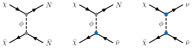
Figure 2: The dominant DM annihilation processes in the mass ranges $m_{\chi}/m_{N}\gtrsim 0.8$ (left), $0.5\lesssim m_{\chi}/m_{N}\lesssim 0.8$ (center), and $m_{\chi}/m_{N}<0.5$ (right). For the center diagram, there is an analogous process for the final state $\bar{N}\nu$. A grey-dot denotes an effective coupling $y_{\rm eff}$ and a blue-square denotes an effective coupling $y_{\rm eff}U_{N\ell}$. The flavor indices have been suppressed.

We begin our phenomenological analysis with a study of the DM relic abundance. Annihilation processes mediated by the scalar $\phi$ play the dominant role. Their rate depends sensitively on the coupling $y_{\rm eff}\!\equiv\!y_{111}$. In our analysis we will consider values of $y_{\rm eff}$ in the range from 1 to $4\pi$. In the early universe, the states of the composite sector are initially in thermal equilibrium with the SM states through the neutrino portal via processes such as $N\nu\leftrightarrow N\nu$ and $NN\leftrightarrow\nu\nu$. The thermal freezeout of $\chi$ can occur through annihilation into three different final states, as shown in  Fig. 2. The relative importance of these processes depends on the ratio $m_{\chi}/m_{N}$:

• $m_{\chi}/m_{N}\geq 0.8$: Note that $\chi$ can be stable even when $m_{\chi}>m_{N}$, as long as $m_{\chi}<m_{\phi}$. The dominant DM annihilation process in this mass range is $\bar{\chi}\chi\to\bar{N}N$. Even though this process cannot proceed at zero temperature if $m_{\chi}<m_{N}$, the kinetic energy of the $\chi$ particles means that it can be important at finite temperatures. From numerical calculations we find that it continues to be the dominant annihilation process for values of $m_{\chi}/m_{N}$ above about 0.8. This is an example of forbidden DM [71]. For this annihilation channel, the thermally averaged cross section is proportional to $y_{\rm eff}^{4}$, which in a strongly coupled theory is expected to be large. Therefore, the annihilation is extremely effective and the observed dark matter abundance is only obtained in a limited region of parameter space.

• $0.5\lesssim m_{\chi}/m_{N}\lesssim 0.8$: In this mass range the dominant annihilation process is $\bar{\chi}\chi\to(\bar{N}\nu,\bar{\nu}N)$. The thermally averaged cross section is proportional to $y_{\rm eff}^{4}U_{N\ell}^{2}$, and the observed DM relic abundance can be obtained at sufficiently small mixing.

• $m_{\chi}/m_{N}<0.5$: In this case the dominant annihilation process is $\bar{\chi}\chi\to\bar{\nu}\nu$ and the thermally averaged cross section is proportional to $y_{\rm eff}^{4}U_{N\ell}^{4}$. Therefore larger mixing angles are favored compared to the mass range above.

We used the package micrOMEGAS-5.2 [72] to determine the relic abundance. In our analysis we were careful to include the coannihilation processes involving higher KK modes. However, for pedagogical reasons, in the discussion below we limit ourselves to an approximate analytic calculation of the DM relic abundance that involves only the lowest KK modes.

We first consider the case when the dominant DM annihilation channel is $\bar{\chi}\chi\to(\bar{N}\nu,\bar{\nu}N)$. In the limit $m_{\phi}^{2}\gg t$, we can approximate the spin-averaged cross section to a single flavor of the final state neutrinos ($\bar{\chi}\chi\to\bar{N}\nu$) as

$$\sum_{\rm spins}\Big{|}{\cal M}(\bar{\chi}\chi\to\bar{N}\nu)\Big{|}^{2}\approx\frac{y_{\rm eff}^{4}U_{N\ell}^{2}(m_{\chi}^{2}-t)(m_{\chi}^{2}+m_{N}^{2}-t)}{4(t-m_{\phi}^{2})^{2}}\;,$$ (4.1)

where $t$ is the Mandelstam variable. After summing over the different flavors and thermally averaging the cross section, we obtain

$$\langle\sigma_{\bar{\chi}\chi\to\bar{N}\nu,N\bar{\nu}}v\rangle\approx\frac{3\,y_{\rm eff}^{4}\,U_{N\ell}^{2}\big{(}4m_{\chi}^{2}-m_{N}^{2}\big{)}^{2}\big{(}4m_{\chi}^{2}+m_{N}^{2}\big{)}}{512\pi m_{\chi}^{4}\big{(}2m_{\chi}^{2}-m_{N}^{2}+2m_{\phi}^{2}\big{)}^{2}}.$$ (4.2)

The Boltzmann equation for the yield ($Y_{\chi}\equiv n_{\chi}/s$) as a function of $x\equiv m_{\chi}/T$ is given by,

$$\frac{dY_{\chi}}{dx}=-\frac{\lambda_{\chi}\left\langle\sigma_{\bar{\chi}\chi\to\bar{N}\nu,N\bar{\nu}}v\right\rangle}{x^{2}}\left[Y_{\chi}^{2}-\bar{Y}_{\chi}^{2}\right]\;,$$ (4.3)

where $n_{\chi}$ is the DM number density and $s$ is the entropy density. In this expression the equilibrium yield $\bar{Y}_{\chi}$ and the parameter $\lambda_{\chi}$ are defined as

$$\bar{Y}_{\chi} \equiv\frac{\bar{n}_{\chi}}{s}=\frac{45}{4\pi^{4}}\frac{g_{\chi}}{g_{\star S}}x^{2}K_{2}(x), \lambda_{\chi} \equiv\frac{x\,s}{H}=\sqrt{\frac{8\pi^{2}}{45}}\,\frac{g_{\star S}}{\sqrt{g_{\star}}}\,M_{\rm Pl}\,m_{\chi}\;.$$ (4.4)

Here $M_{\rm Pl}$ is the reduced Planck mass, $H$ is the Hubble rate and $K_{2}(x)$ is the modified Bessel function. The parameters $g_{\star}$ and $g_{\star S}$ represent the effective number of relativistic degrees of freedom for the energy and entropy densities of radiation respectively, while $g_{\chi}$ denotes the number of degrees of freedom in DM.

Equivalent expressions for the $\bar{\chi}\chi\to\bar{\nu}\nu$ annihilation channel are

$$\sum_{\rm spins}\Big{|}{\cal M}(\bar{\chi}\chi\to\bar{\nu}\nu)\Big{|}^{2}\approx\frac{y_{\rm eff}^{4}U_{N\ell}^{4}(m_{\chi}^{2}-t)^{2}}{4(m_{\phi}^{2}-t)^{2}}\;.$$ (4.5)

and

$$\langle\sigma_{\bar{\chi}\chi\to\bar{\nu}\nu}\,v\rangle\approx\frac{3\,y_{\rm eff}^{4}\,U_{N\ell}^{4}\,m_{\chi}^{2}}{32\pi\,m_{\phi}^{4}}\;.$$ (4.6)

The present-day DM relic density can be obtained by solving the Boltzmann equation,

$$\Omega_{\chi}h^{2}=\frac{h^{2}s_{0}}{\rho_{\text{cr}}}m_{\chi}Y_{\chi}^{(0)}=2.742\times 10^{8}\left(\frac{m_{\chi}}{\text{GeV}}\right)Y_{\chi}^{(0)},$$ (4.7)

where $Y_{\chi}^{(0)}$ is the DM yield, $s_{0}=2970\,{\rm cm}^{-3}$ is the total entropy density today, and $\rho_{\text{cr}}=1.054\times 10^{-5}h^{2}\;\hbox{GeV}\,{\rm cm}^{-3}$ is the critical density. The observed DM relic abundance is $\Omega_{\rm obs}h^{2}=0.12\pm 0.012$ [73].

In Fig. 3 we show the evolution of the DM relic abundance as a function of $x=m_{\chi}/T$ for a benchmark spectrum with $m_{\chi}=0.6\;\hbox{GeV}$, $m_{N}=\Lambda=1\;\hbox{GeV}$ and $m_{\phi}=1.7\;\hbox{GeV}$, the dominant annihilation channel being $\bar{\chi}\chi\to(\bar{N}\nu,\bar{\nu}N)$. We have taken $y_{\rm eff}=\sqrt{4\pi}$, and considered two values of the mixing, $|U_{N\ell}|^{2}=10^{-6}$ (red) and $10^{-8}$ (blue). The solid lines result from the approximate analytic calculation presented above, whereas the dots show the numerical results obtained with micrOMEGAS, which include the effects of the higher KK modes. Fig. 4 shows an equivalent plot for a benchmark wherein $m_{\chi}/m_{N}=0.4$, $\Lambda=m_{N}/1.11=1\;\hbox{GeV}$ and $m_{\phi}=1.7\;\hbox{GeV}$, the dominant annihilation channel being $\bar{\chi}\chi\to\bar{\nu}\nu$. With the same value for $y_{\rm eff}$, we consider larger values for the mixing $|U_{N\ell}|^{2}=10^{-3}$ (red) and $10^{-4}$ (blue). This is necessary because of the extra factors of the mixing that appear in the corresponding annihilation cross section. The good agreement between the analytic and numerical results confirms that neglecting the higher KK-modes is a good approximation.

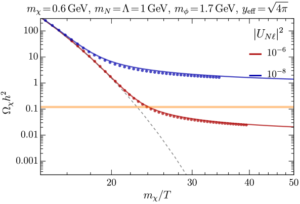
Figure 3: The DM relic abundance as a function of $x=m_{\chi}/T$ is shown for a benchmark spectrum with the parameters $m_{\chi}=0.6\;\hbox{GeV}$, $m_{N}=\Lambda=1\;\hbox{GeV}$, $m_{\phi}=1.7\;\hbox{GeV}$ and two choices of the mixing angle, $|U_{N\ell}|^{2}=10^{-6}$ (red) and $10^{-8}$ (blue). The dominant annihilation channel is $\bar{\chi}\chi\to(\bar{N}\nu,\bar{\nu}N$). The dots show the numerical results obtained using micrOMEGAS. The dashed-grey line represents the equilibrium density and the orange horizontal band corresponds to the observed DM relic density.

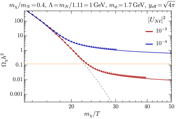
Figure 4: The DM relic abundance as a function of $x=m_{\chi}/T$ is shown for a benchmark spectrum with $m_{\chi}/m_{N}=0.4$, $\Lambda=m_{N}/1.11=1\;\hbox{GeV}$, $m_{\phi}=1.7\;\hbox{GeV}$ and two choices of the mixing angle, $|U_{N\ell}|^{2}=10^{-3}$ (red) and $10^{-4}$ (blue). The dominant annihilation channel is $\bar{\chi}\chi\to\bar{\nu}\nu$. The dots show the numerical results obtained using micrOMEGAS. The dashed-grey line represents the equilibrium density and the orange horizontal band corresponds to the observed DM relic density.

4.2 Direct Detection

Direct detection experiments are significantly less sensitive to composite DM that couples to the SM through the neutrino portal than to conventional WIMPs. This is because the DM-nucleon interactions are induced only at the loop level and are further suppressed by the small mixing between the SM neutrinos and their singlet counterparts. While this has the effect of weakening the constraints on the model, it of course also makes the model more challenging to discover in direct detection experiments. In particular, we will show below that in a large region of parameter space, the DM-nucleon cross section lies below the neutrino floor.

The loop diagram shown in Fig. 5 leads to an effective $Z\bar{\chi}\chi$ vertex of the form

$$g_{Z\bar{\chi}\chi}\,Z_{\mu}\bar{\chi}\gamma^{\mu}P_{L}\chi\;,$$ (4.8)

where $P_{L}$ is the projection operator for left-handed states. This gives rise to DM scattering off nuclei via $Z$ exchange. In what follows, we calculate the cross section for this process, working in the physical mass eigenbasis. Although an effective coupling to the Higgs boson is also induced, the Higgs exchange contribution to direct detection is additionally suppressed by the small coupling of the Higgs to nuclei, and can therefore safely be neglected. The effective coupling $g_{Z\bar{\chi}\chi}$ is given by

$$g_{Z\bar{\chi}\chi}=\sum_{n,r,s}\frac{U_{N_{r}\ell}\,U_{N_{s}\ell}\,y_{r1n}\,y_{s1n}}{16\pi^{2}}\frac{3g\,m_{N_{r}}m_{N_{s}}}{2\cos\theta_{W}}\,C_{0}\left(m_{\chi}^{2},m_{\chi}^{2},q^{2};m_{N_{r}},m_{\phi_{n}},m_{N_{s}}\right),$$ (4.9)

where the sum is over the KK modes of $N$ and $\phi$. Here $C_{0}$ is the scalar Passarino–Veltman three-point function as defined in Ref. [74] and $q^{\mu}$ is the four-momentum carried by the $Z$. Since each term in the sum is proportional to the fermion masses in the loop, the contribution from the light neutrinos is negligible. All the terms in the sum are suppressed by the squares of the mixing parameters. On the other hand, since the couplings $y_{r1n}$ arise from strong dynamics, they are expected to be large.

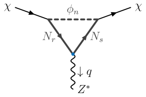
Figure 5: The figure shows the Feynman diagram for the loop-induced coupling of DM to the $Z$-boson. The subscripts on the fields in the loop denote the KK modes. The blue dot denotes the coupling of the $Z$ in the mass eigenbasis to $N_{r}$ and $N_{s}$, which is suppressed by mixing angles.

The contribution to $g_{Z\bar{\chi}\chi}$ from just the lowest KK-modes of $N$ and $\phi$ in the limit $m_{\phi}\gg m_{N}$ is given by

$$g_{Z\bar{\chi}\chi}=\frac{U_{N\ell}^{2}\,y_{\rm eff}^{2}}{8\pi^{2}}\frac{g}{2\cos\theta_{W}}\frac{m_{N}^{2}}{m_{\phi}^{2}}\bigg{[}1+\ln\bigg{(}\frac{m_{N}^{2}}{m_{\phi}^{2}}\bigg{)}\bigg{]}.$$ (4.10)

However, we find that including the higher KK-modes of $N$ in the loop corrects this expression by an order one factor. We therefore provide formulas for the general terms appearing in the sum. In particular, in the limit $q^{2}\ll m_{\chi}^{2}$, one can simplify the above Passarino–Veltman $C_{0}$ function. For $r=s$, the $C_{0}$ function simplifies to

$$C_{0}(m_{\chi}^{2},m_{\chi}^{2},0;m_{N_{r}},m_{\phi_{n}},m_{N_{r}}) \!=\!-\frac{(m_{\chi}^{2}-m_{N_{r}}^{2}+m_{\phi_{n}}^{2})\Lambda\big{(}m_{\chi}^{2},m_{N_{r}},m_{\phi_{n}}\big{)}}{\lambda\big{(}m_{\chi}^{2},m_{N_{r}}^{2},m_{\phi_{n}}^{2}\big{)}}-\frac{1}{2m_{\chi}^{2}}\ln\!\!\bigg{(}\frac{m_{N_{r}}^{2}}{m_{\phi_{n}}^{2}}\bigg{)}.$$ (4.11)

For $r\neq s$, we get instead,

$$\frac{1}{m_{N_{r}}^{2}-m_{N_{s}}^{2}}\bigg{[}\bigg{(}\Lambda\left(m_{\chi}^{2},m_{\phi_{n}},m_{N_{r}}\right)-\frac{(m_{\chi}^{2}+m_{N_{r}}^{2}-m_{\phi_{n}}^{2})}{2m_{\chi}^{2}}\ln\!\Big{(}\frac{m_{N_{r}}^{2}}{m_{\phi_{n}}^{2}}\Big{)}\bigg{)}-\left(r\leftrightarrow s\right)\bigg{]}.$$ (4.12)

The Källén kinematic triangular polynomial $\lambda(a,b,c)$ and the function $\Lambda(m_{0}^{2},m_{i},m_{j})$ appearing in the formulae above are defined as

$$\lambda\big{(}a,b,c\big{)} \equiv a^{2}+b^{2}+c^{2}-2ab-2bc-2ca\,,$$ (4.13)

$$\Lambda(m_{0}^{2},m_{i},m_{j}) \equiv\frac{1}{m_{0}^{2}}\sqrt{\lambda\big{(}m_{0}^{2},m_{i}^{2},m_{j}^{2}\big{)}}\ln\!\bigg{(}\frac{m_{i}^{2}+m_{j}^{2}-m_{0}^{2}+\sqrt{\lambda\big{(}m_{0}^{2},m_{i}^{2},m_{j}^{2}\big{)}}}{2m_{i}m_{j}}\bigg{)}.$$ (4.14)

The DM–nucleon spin-independent cross section $\sigma_{\chi n}^{\rm SI}$ mediated via $Z$ exchange is given by,

$$\sigma_{\chi n}^{\rm SI}=\frac{g^{2}g_{Z\chi\bar{\chi}}^{2}}{64\pi\cos^{2}\theta_{W}m_{Z}^{4}}\bigg{(}\frac{m_{\chi}m_{n}}{m_{\chi}+m_{n}}\bigg{)}^{2}\left[\left(1+\frac{Z}{A}\right)V_{u}+\left(2-\frac{Z}{A}\right)V_{d}\right]^{2},$$ (4.15)

where $m_{n}$ is the nucleon mass, $Z/A$ is the ratio of the atomic and mass numbers of the target nucleus, and $V_{f}\!=\!(2T^{3}_{f}-4Q_{f}\sin^{2}\theta_{W})$ for a fermion $f$ with electric charge $Q_{f}$ and isospin number $T^{3}_{f}$. Using this cross section, we plot in Figs. 6 and 7, for a set of benchmark model parameters, the mixing angles as a function of $m_{\chi}$ that correspond to the current exclusion from the first results of LZ experiment [62] and the expected sensitivity of the XENONnT experiment [53]. Also shown is the mixing angle that would result in a cross section equal to the neutrino floor [53].

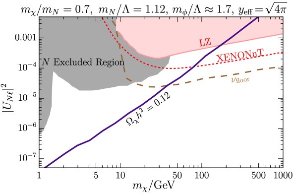
Figure 6: We plot the current exclusion from the LZ experiment (2022) [62], along with the expected sensitivity of the XENONnT experiment [53] and the mixing angle corresponding to the neutrino floor [53], for the benchmark model parameters listed at the top of the figure. The gray-shaded region is ruled out by a variety of collider and beam dump searches. The solid blue curve represents the contour of $y_{\rm eff}=\sqrt{4\pi}$ which produces the observed DM relic abundance.

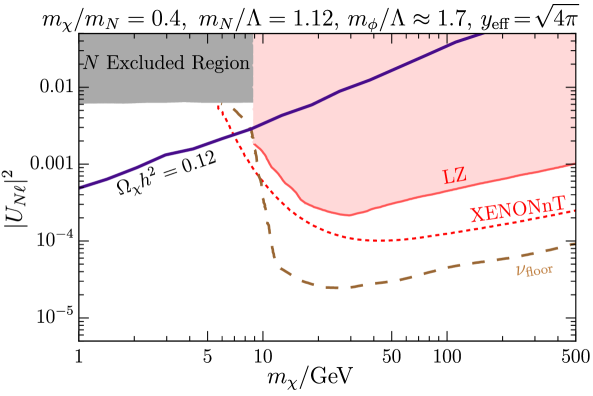
Figure 7: We plot the current exclusion from the LZ experiment [62], along with the expected sensitivity of the XENONnT experiment [53] and the mixing angle corresponding to the neutrino floor [53], for the benchmark model parameters listed at the top of the figure. The gray-shaded region is ruled out by a variety of collider searches. The solid blue curve produces the observed DM relic abundance for $y_{\rm eff}=\sqrt{4\pi}$.

4.3 Indirect Detection

The indirect detection signals of this class of models are very different for the $(\bar{N}\nu,\bar{\nu}N)$ and $\bar{\nu}\nu$ annihilation channels. In the case when the primary annihilation channel is $\bar{\chi}\chi\to(\bar{N}\nu,\bar{\nu}N)$, the singlet neutrino in the final state decays to leptons, neutrinos, and hadrons with ${\mathcal{O}}(1)$ branching ratios. When all the unstable particles have decayed, a continuum spectrum of electrons, positrons, photons, and neutrinos is produced. On average, their energies do not significantly exceed $m_{N}/3$, since the $N$-decay is 3-body. There are strong astrophysical and cosmological constraints on these final states from indirect detection experiments. In particular, cosmic microwave background (CMB) measurements provide a robust probe of DM annihilations to energetic electrons and photons around the recombination epoch. The energy injected into the plasma by annihilations of DM particles modifies the ionization history as well as temperature and polarization anisotropies. The measurements of the CMB by the Planck collaboration [73] set stringent constraints on DM annihilation for GeV-scale or lighter DM. There are also constraints on this class of theories from present-day observations of gamma rays from the galactic center and from dwarf galaxies. In the case of annihilation to $\bar{\nu}\nu$, none of these constraints apply.

Since the DM particles are nonrelativistic, it follows that for both the $(\bar{N}\nu,\bar{\nu}N)$ and $\bar{\nu}\nu$ channels, the SM neutrinos produced in the annihilation process are monochromatic. The neutrino energy is given by $E_{\nu}=m_{\chi}(1-m_{N}^{2}/4m^{2}_{\chi})$ for the $(\bar{N}\nu,\bar{\nu}N)$ annihilation mode and $E_{\nu}=m_{\chi}$ for the $\bar{\nu}\nu$ annihilation mode. A monochromatic neutrino line is a striking signature for indirect detection experiments. After identifying the regions in parameter space that are consistent with the CMB and gamma-ray constraints, we will estimate the reach for such a signature in Sec. 4.3.3.

4.3.1 CMB constraints

As mentioned above, CMB observations constrain the $(\bar{N}\nu,\bar{\nu}N)$ annihilation channel since the subsequent decays of composite singlet neutrinos inject energy into the intergalactic medium (IGM) at the recombination epoch. The constraints from the Planck collaboration [73] are expressed as channel-dependent upper-bounds on the thermally averaged annihilation cross section $\langle\sigma v\rangle$ at 95% C.L.,

$$f_{\!\rm eff}(m_{\chi})\frac{\langle\sigma v\rangle}{m_{\chi}}<3.2\times 10^{-28}\,{\rm cm^{3}\,s^{-1}}\;\hbox{GeV}^{-1},$$ (4.16)

where $f_{\!\rm eff}(m_{\chi})$ is the effective fraction of energy transferred to the IGM from DM annihilation at a redshift $z\sim 600$ where the CMB anisotropy data is most sensitive. In our model, $\langle\sigma v\rangle\sim{\rm few}\times 10^{-26}\,{\rm cm^{3}\,s^{-1}}$ in order to produce the observed DM relic abundance. Therefore, the CMB constraint can be translated directly into a limit on $f_{\!\rm eff}(m_{\chi})$, which is a function of the DM mass and the final state particles that result from the DM annihilation process.

Since the Planck limits are most sensitive to electrons and photons in the final state, we calculate $f_{\!\rm eff}(m_{\chi})$ as a weighted average of the electron and photon spectra $(dN_{e^{-},\gamma}/dE)$ predicted by our model for the DM annihilation process $\bar{\chi}\chi\to N\bar{\nu}$ as,

$$f_{\!\rm eff}(m_{\chi})=\frac{1}{4m_{\chi}}\int_{0}^{m_{\chi}(1+m_{N}^{2}/4m_{\chi}^{2})}dEE\bigg{[}2f_{\!\rm eff}^{e^{-}}(E)\frac{dN_{e^{-}}}{dE}+f_{\!\rm eff}^{\gamma}(E)\frac{dN_{\gamma}}{dE}\bigg{]}\;.$$ (4.17)

To compute this we employ the results of Ref. [75], which provides data on $f_{\!\rm eff}^{e^{\!-},\gamma}(E)$, the fraction of energy transferred to the IGM for energies in the range [keV–TeV]. We use pythia8 [76] to calculate the photon and electron spectra arising from the DM annihilation $\bar{\chi}\chi\to(\bar{N}\nu,\bar{\nu}N)$. This incorporates the effects of showering and hadronization in the decays of $N$ to SM states. We sum over all the flavors of $N$ in the final state. In Fig. 8 we show the photon (left-panel) and electron (right-panel) energy spectra for a few benchmark values of the DM mass.

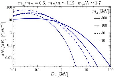
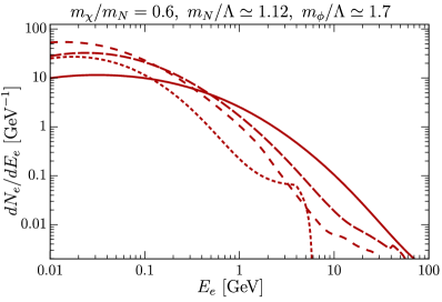
Figure 8: The left (right) panel of this figure shows the photon (electron) energy spectrum arising from the annihilation channel $\bar{\chi}\chi\to N\nu$ and the subsequent decay of $N$.

In Fig. 9 we plot our result for the fractional annihilation energy transferred per unit DM mass, $f_{\!\rm eff}(m_{\chi})/m_{\chi}$, as function of $m_{\chi}$. The horizontal dashed orange line corresponds to the Planck constraint from Eq. (4.16). As can be seen in this figure, the Planck CMB constraint excludes DM annihilating to the $(\bar{N}\nu,\bar{\nu}N)$ final states for $m_{\chi}\lesssim 4\;\hbox{GeV}$. Therefore for DM masses lower than this value, only the annihilation channel to $\bar{\nu}\nu$, where no energy is injected into the IGM, is consistent with CMB bounds. We also show the sensitivity of future CMB-S4 experiments as the horizontal dotted orange line. This projected sensitivity is based on the analysis of Ref. [77], where it is shown that the most optimistic configuration of the CMB-S4 experiment could be sensitive to $f_{\!\rm eff}(m_{\chi})\langle\sigma v\rangle/m_{\chi}\sim 1.17\times 10^{-28}\,{\rm cm^{3}\,s^{-1}}\;\hbox{GeV}^{-1}$ at 95% C.L. Hence the resulting projected exclusion reach from CMB-S4 on the DM mass is $m_{\chi}\sim 10\;\hbox{GeV}$ for the $(\bar{N}\nu,\bar{\nu}N)$ annihilation channel.

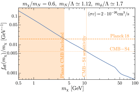
Figure 9: The blue curve shows $f_{\!\rm eff}(m_{\chi})/m_{\chi}$, the fraction of energy transferred to the IGM due to DM annihilations around the time of recombination divided by $m_{\chi}$, as a function of $m_{\chi}$, for the benchmark spectrum listed above the figure. The dominant annihilation channel is $\chi\bar{\chi}\to(\bar{N}\nu,\bar{\nu}N)$. The horizontal dashed line represents the 95% constraint on this quantity from the Planck collaboration [73] for $\langle\sigma v\rangle=2.2\times 10^{-26}\,{\rm cm^{3}\,s^{-1}}$. As a result, this annihilation mode is ruled out for DM masses in the shaded region. The horizontal dotted line shows the projected sensitivity of CMB-S4 at 95% C.L., which implies a sensitivity to DM annihilation in this channel up to $m_{\chi}\sim\!10\;\hbox{GeV}$.

4.3.2 Gamma Ray Constraints

In this subsection, we consider constraints on this class of models based on measurements of gamma rays from the galactic center (GC) of the Milky Way and from dwarf spheroidal satellite (dSphs) galaxies. In recent years these measurements have provided powerful bounds on DM models. GC searches have the advantage of a potentially large signal component, especially if the DM profile is cuspy, but suffer from large astrophysical backgrounds, while dSphs have much lower backgrounds but also contain a smaller signal component.

Galactic Center (GC):

We employ the Fermi-LAT Fourth Source Catalog (4FGL) [78] with 8 years of data for our analysis of the GC and follow the procedure adopted in Ref. [79]. Assuming universality among the different flavors of composite singlet neutrinos, the expected photon flux per unit energy from DM annihilation is given by,

$$\frac{d\Phi_{\gamma}}{dE_{\gamma}}=\frac{1}{4\pi}\frac{\langle\sigma v\rangle}{4m_{\chi}^{2}}\frac{dN_{\gamma}}{dE_{\gamma}}J,$$ (4.18)

where $\langle\sigma v\rangle$ is the total thermally averaged cross section. The calculation of the photon energy spectrum using pythia8 has been described in the previous subsection, with the result shown in the left panel of Fig. 8. The $J$-factor is given by

$$J\equiv\int\!d\Omega\int_{0}^{\ell_{\max}}d\ell\,\rho_{\chi}^{2}(\ell),$$ (4.19)

where $d\Omega$ is integrated over the region of interest and the $d\ell$ integral is over the line of sight. We consider two different DM density profiles, the standard Navarro-Frenk-White (NFW) profile [80] and a cored DM halo profile proposed by Read et al. [81]. The standard NFW profile is given by

$$\rho_{\chi}(r)=4\,\rho_{s}\bigg{(}\frac{r_{s}}{r}\bigg{)}\bigg{(}1+\frac{r}{r_{s}}\bigg{)}^{-2},$$ (4.20)

where $r$ is the distance from the GC and $\rho_{s}$ is the DM density at the scale radius $r_{s}=20\,{\rm kpc}$. We take $\rho_{s}=0.065\,{\rm GeV/cm^{3}}$, which gives the local DM density as $\rho(r_{0})=0.3\,{\rm GeV/cm^{3}}$ for $r_{0}=8.5\,{\rm kpc}$, the distance of the sun from the center of the Milky Way. The line of sight $\ell$ is related to $r$ by

$$r=\sqrt{r_{0}^{2}-2\ell r_{0}\cos\theta+\ell^{2}},$$ (4.21)

where $\theta$ is the angle between the GC and the line of sight. We take the integration limit $\ell_{\rm max}$ in Eq. (4.19) to satisfy

$$\ell_{\max}=\sqrt{r_{\text{MW}}^{2}-r_{0}^{2}\,\sin^{2}\theta}+r_{0}\cos\theta,$$ (4.22)

where $r_{\text{MW}}\sim 40\,{\rm kpc}$ is the size of the Milky Way halo.

For the cored halo profile, we employ a core radius $r_{c}=1\,{\rm kpc}$. The mass of the cored profile $M_{\rm core}(r)$ asymptotically approaches that of the NFW profile $M_{\rm NFW}(r)$ in the outer regions as [79, 81],

$$M_{\rm core}(r)=M_{\rm NFW}(r)\tanh(r/r_{c}).$$ (4.23)

In Fig. 10 we present the results of our analysis. For the cored DM halo profile, shown as the solid blue curve, we find that the range of $m_{\chi}$ between 2 GeV and 20  GeV is excluded at 95% C.L. for the benchmark case $m_{\chi}/m_{N}=0.7$. For the NFW DM halo profile, shown as the dashed-blue curve, the exclusion range is found to be between $m_{\chi}=1\;\hbox{GeV}$ and $m_{\chi}=30\;\hbox{GeV}$. As expected, the limits from the NFW profile are somewhat stronger.

Dwarf Spheroidal Satellite Galaxies:

We also calculate the constraints from a set of dSphs galaxies with well-determined $J$-factors. We employ the log-likelihood profiles for the dSphs from Fermi-LAT data [82, 83] and we take the uncertainties in the $J$-factors from [84]. These uncertainties are calculated from fits to the stellar kinematic data using generalized NFW profiles. From the analysis, we find an exclusion at 95% CL for DM in the mass range $m_{\chi}\!\sim\!(5-10)\;\hbox{GeV}$ for $m_{\chi}/m_{N}=0.7$. This is shown in Fig. 10 as the green curve. This limit is weaker than the bound on gamma rays from the GC.

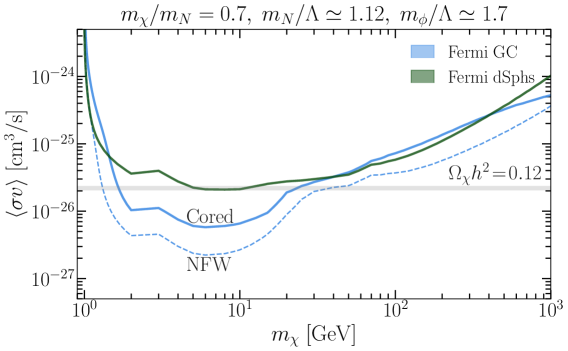
Figure 10: We show the 95% CL limit on $\langle\sigma v\rangle$ from Fermi-LAT GC (blue curves) and dSphs (green curve) as a function of the DM mass $m_{\chi}$ for the benchmark value $m_{\chi}/m_{N}=0.7$, the dominant annihilation channel being $\bar{\chi}\chi\to(\bar{N}\nu,\bar{\nu}N)$. The horizontal gray line denotes the value required for the observed DM relic abundance $\Omega_{\chi}h^{2}\simeq 0.12$. The solid and dashed blue curves correspond to cored and NFW DM halo profiles respectively, based on data from Fermi-LAT fourth source catalogs.

4.3.3 Neutrino Line Signal

Several experiments including SuperK [85], IceCube [86], and ANTARES [87] have placed limits on a neutrino line signal from DM annihilations. Their data has also been reanalyzed by independent groups seeking to extend the constraints to lower values of the DM mass [88, 89, 90, 91]. Recently, the KamLAND experiment [92] also reported a bound on DM annihilation to neutrinos in the low mass range $m_{\chi}\sim[8-30]\;\hbox{MeV}$. In the top half of Table 2, we summarize a variety of experimental constraints on the thermally averaged cross section $\langle\sigma v\rangle$, along with the mass range for which they are applicable.

For an annihilation cross section compatible with obtaining the correct DM relic abundance, these experiments are only sensitive when the DM mass is below a GeV, because then the DM number density is high and therefore the flux in the neutrino line is large. Since we have concluded that the $(\bar{N}\nu,\bar{\nu}N)$ annihilation channel is ruled out for light DM masses by CMB constraints, in this section we limit our attention to the $\bar{\nu}\nu$ annihilation channel.

The existing bounds only go down to values of $\langle\sigma v\rangle$ of order $10^{-25}\,{\rm cm^{3}/s}$, which is still significantly above the value required to obtain the observed DM density. However, future experiments such as HyperK [93], JUNO [61] and DUNE [94] are projected to have the necessary level of sensitivity to detect thermal relic DM in the mass range $15\;\hbox{MeV}$ - $90\;\hbox{MeV}$. In the lower half of Table 2 we report recent 90% projections on the reach of these future experiments from independent analyses [95, 89, 90, 91]. In our numerical analysis below, we make use of the most optimistic projections for these experiments.

Experiment/analysis	DM mass range	Best upper-limit $\langle\sigma v\rangle$
SuperK [85]	$1-10^{4}\;\hbox{GeV}$	$1.2\times 10^{-24}\,{\rm cm^{3}/s}$
IceCube [86]	$5-200\;\hbox{GeV}$	$3.5\times 10^{-25}\,{\rm cm^{3}/s}$
ANTARES [87]	$50-10^{5}\;\hbox{GeV}$	$1.5\times 10^{-24}\,{\rm cm^{3}/s}$
KamLAND [92]	$8-21\;\hbox{MeV}$	$5\times 10^{-25}\,{\rm cm^{3}/s}$
HyperK [90, 91]	$17\;\hbox{MeV}-50\;\hbox{GeV}$	$3\times 10^{-26}\,{\rm cm^{3}/s}$
JUNO [89, 90]	$10-80\;\hbox{MeV}$	$4\times 10^{-26}\,{\rm cm^{3}/s}$
DUNE [89, 90]	$10-80\;\hbox{MeV}$	$3\times 10^{-26}\,{\rm cm^{3}/s}$

Table 2: Existing (top half) and projected future (bottom half) experimental limits (90% C.L.) on DM annihilating directly to neutrinos, along with the corresponding DM mass range.

In what follows, we map the sensitivity of these future experiments to the parameter space of our model. Since the sensitivity projections for different experiments use somewhat different assumptions (about the DM density profile, etc.), we will also need to make all dependencies on these assumptions explicit, so that the sensitivity of different experiments can be directly compared.

Note that most experimental searches are performed for a specific neutrino flavor. Assuming universality among neutrino flavors, the expected flux on the Earth for each neutrino and antineutrino flavor from DM annihilation is given by,

$$\frac{d\Phi_{\nu}}{dE_{\nu}}=\frac{1}{4\pi}\frac{\langle\sigma v\rangle}{4m_{\chi}^{2}}\frac{1}{3}\frac{dN_{\nu}}{dE_{\nu}}J,$$ (4.24)

where the neutrino spectrum is mono-energetic, i.e.

$$\frac{dN_{\nu}}{dE_{\nu}}=\kappa_{\nu}\frac{m_{\chi}}{E_{\nu}^{2}}\,\delta\big{(}1-E_{\nu}/m_{\chi}\big{)}\;.$$ (4.25)

Here $\kappa_{\nu}=2$ for the annihilation channel $\bar{\chi}\chi\to\bar{\nu}\nu$, and the $J$-factor is given in Eq. (4.19). Note that using a more cuspy DM profile results in a larger $J$-factor, and therefore a stronger DM signal. For an NFW DM halo profile, we obtain an all-sky $J$-factor of $J\sim\!9\times 10^{22}\,{\rm GeV^{2}/cm^{5}}$. In Fig. 11 we present the resulting experimental constraints and projections [95, 89, 90, 91]. As shown in this figure, the sensitivity of these experiments can reach the thermal relic cross section in the DM mass range 10–100 MeV. Unfortunately, this mass range is disfavored by the existing constraints from beam dumps and the bounds on DM self-interactions.

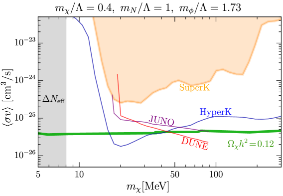
Figure 11: We plot the projected indirect detection constraint from the SuperK experiment (shaded orange region), along with future experiments (colored curves). Note that the sensitivities of SuperK and HyperK in this low mass range are based on Refs. [90, 91], not on the official results from the collaborations on which the numbers listed in Table 2 are based. All the constraints correspond to a standard NFW DM density profile. The green line denotes the annihilation cross section that reproduces the observed relic abundance. At the lower end of the DM mass range, $\Delta N_{\rm eff}$ bounds from CMB and BBN disfavor values of $m_{\chi}$ below $8\;\hbox{MeV}$ [96, 97, 98].

4.4 Results

We are now ready to combine the conclusions of the different parts of this section and identify viable regions in the parameter space of our model. For the case when the dominant annihilation channel is $\bar{\chi}\chi\to(\bar{N}\nu,\bar{\nu}N)$, we present all the relevant constraints in Fig. 12, for the choices of $\Delta_{N}=\Delta_{\widehat{N}}=9/4$ (corresponding to $m_{N}\simeq 1.12\,\Lambda$) and $\Delta_{\chi}=\Delta_{\widehat{\chi}}\simeq 2$ (corresponding to $m_{\chi}=0.7\,m_{N}$). At each point, $y_{\rm eff}$ has been chosen such that the correct DM relic abundance is obtained. The inequalities in Eq. (2.16) are satisfied throughout this parameter region so that realistic neutrino masses can be obtained. The various shaded regions in the plot are excluded (see the figure caption for more detailed information on each constraint). The DM self-interaction constraint from Eq. (2.26) for this benchmark point is only relevant for $m_{\chi}\lesssim 0.5\;\hbox{GeV}$, and has therefore not been shown. The gray-shaded region corresponds to the bounds on HNLs from colliders and beam dumps. The reason that this constraint weakens for larger masses is that the $N$ particles become too heavy to be produced from on-shell $W$ decays. Therefore the signal cross section drops precipitously while the background cross section falls more gradually, resulting in greatly reduced experimental sensitivity. We see from the plot that near-future direct detection experiments will have sensitivity for values of the DM mass above about 40 GeV. In the longer term, DM masses as low as 20 GeV may be accessible to direct detection. In the next section, we will evaluate the reach of future collider searches in this parameter space.

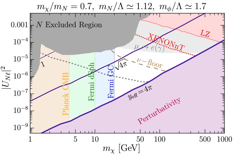
Figure 12: We show the constraints on our model in the parameter space of DM mass and the $N$-$\nu$ mixing angle for the benchmark parameters listed above the figure. The dominant annihilation channel is $\bar{\chi}\chi\to(N\bar{\nu},\bar{N}\nu)$, and $y_{\rm eff}$ at each point has been chosen to reproduce the correct DM relic abundance. Contours of constant $y_{\rm eff}$ are shown as purple lines. The grey-shaded region is excluded by collider, beam dump, and astrophysical constraints [35]. The light-gray region corresponds to the current exclusion from the lepton flavor violating processes $\mu\to e$ conversion and $\mu\to e\gamma$ under the assumption of maximal lepton mixing, whereas the dotted gray curve represents the projected future sensitivity from these processes. The orange-shaded region on the left is excluded at 95% C.L. by Planck CMB data as discussed in Sec. 4.3.1. The red-shaded region in the top-right corner is excluded by the direct detection constraint from the LZ (2022) experiment as discussed in Sec. 4.2. The red-dotted curve shows the projected sensitivity of the LZ/XENONnT experiment and the brown-dashed curve corresponds to the mixing angle below which the signal in direct detection experiments would fall below the neutrino floor. The gamma-ray constraints of Fig. 10 are depicted by the green and blue shaded regions. The purple shaded region corresponds to $y_{\rm eff}>4\pi$ and is accordingly disfavored by unitarity considerations.

In this plot we have included the constraints (light-gray region) from the lepton flavor violating processes $\mu\to e$ conversion and $\mu\to e\gamma$, after relaxing the assumption that the couplings of the composite singlet neutrinos to the SM are flavor diagonal. Then, at the one-loop level, they contribute to these lepton flavor violating processes [35]. The light-gray region is the current constraint in the limit that we have maximal mixing between the $\mu$ and $e$ flavors, i.e. $\big{|}\!\sum_{n}U_{N_{n}\mu}^{\ast}U_{N_{n}e}\!\big{|}=\big{|}U_{N\ell}\big{|}^{2}$, where the sum over $n$ is over the KK modes in the loop. We adopt the strongest constraint from the MEG experiment [99] for the $\mu\to e\gamma$ process and from the SINDRUM II experiment [100] for $\mu\to e$ conversion. In the near future the Mu2e [101] and COMET [102] experiments will be searching for $\mu\to e$ conversion. The future constraints in the absence of a signal are shown in Fig. 12 as the dotted-gray curve. Note that relaxing the assumption of maximal lepton mixing would lead to a weakening of the corresponding constraints.

For the case when the primary annihilation channel is $\bar{\chi}\chi\to\bar{\nu}\nu$, we present the relevant constraints in Fig. 13, for the choices of $\Delta_{N}=\Delta_{\widehat{N}}=9/4$ (corresponding to $m_{N}\simeq 1.12\,\Lambda$) and $m_{\chi}/m_{N}=0.4$ (corresponding to $\Delta_{\chi}\simeq 7/4$). As before, $y_{\rm eff}$ at each point has been chosen to obtain the correct DM relic abundance, and the entire parameter region in the plot is compatible with Eq. (2.16). The shaded regions correspond to exclusions, except for the red and blue vertical hatched bands denoting the regions of sensitivity to future neutrino-line searches, as discussed in Sec. 4.3.3. Unfortunately, these regions are already excluded by the existing collider and beam dump bounds. Moreover, the DM self-interaction constraint in Eq. (2.26), i.e. $\sigma_{\rm self}/m_{\chi}\!\lesssim\!0.7\,{\rm cm^{2}/g}$, leads to a lower bound on the DM masses shown as the green solid band. In obtaining this bound we have taken $\kappa_{\chi}\simeq y_{\rm eff}^{2}$ to be consistent with large-$\mathcal{N}$ counting. We see that the DM self-interaction constraint also disfavors a part of the region where future HyperK and DUNE searches are sensitive to a neutrino line signal.

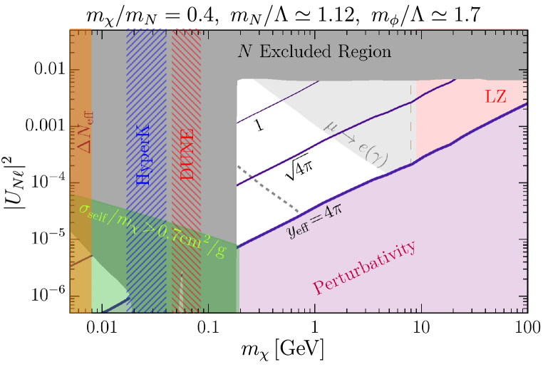
Figure 13: This plot shows the constraints on our model in the parameter space of DM mass and the $N$-$\nu$ mixing angle for the benchmark parameters listed above the figure. The dominant annihilation channel is $\bar{\chi}\chi\to\bar{\nu}\nu$, and $y_{\rm eff}$ at each point has been chosen to reproduce the correct DM relic abundance. Contours of constant $y_{\rm eff}$ are shown as purple lines. The grey-shaded region is excluded by beam dump and electroweak precision constraints [103]. The light-gray region corresponds to the current exclusion from the lepton flavor violating processes $\mu\to e$ conversion and $\mu\to e\gamma$ under the assumption of maximal lepton mixing, whereas the dotted gray curve represents the projected future sensitivity from these processes. The red-shaded region in the top-right corner is excluded by the direct detection constraint from the LZ (2022) experiment as discussed in Sec. 4.2 and to the left of the brown-dashed verticle line the direct detection experiments would fall below the neutrino floor. The orange-shaded region on the left is excluded by the CMB and BBN constraints on the effective number of relativistic degrees of freedom $\Delta N_{\rm eff}$. The blue and red vertical hatched bands are projected regions where future HyperK and DUNE experiments, respectively, have sensitivity for the detection of a neutrino-line. The green-shaded region is excluded due to DM self-interaction constraints discussed in Sec. 2.3. The purple shaded region corresponds to $y_{\rm eff}>4\pi$ and is disfavored by unitarity considerations.

5 Collider Phenomenology

Let us now turn our attention to the collider signatures of this class of models. As described earlier, composite singlet neutrinos can be produced at colliders via the neutrino portal. When $m_{\chi}<M_{N}/2$ (i.e. when the annihilation channel is $\chi\bar{\chi}\to\nu\bar{\nu}$), $N$ can decay fully invisibly into $\chi\bar{\chi}\nu$. This decay occurs via the $N\bar{N}\chi\bar{\chi}$ interaction in the hidden sector, with an insertion of $N$-$\nu$ mixing. Since any $N$ decay channels into SM final states also require at least one mixing angle (in the form of the portal coupling), and are further suppressed by $G^{2}_{F}m^{4}_{N}$ due to the off-shell $W$ or $Z$ bosons that mediate the process, the decays to $\chi\bar{\chi}\nu$ will completely dominate over the SM decays. Therefore, in this region of parameter space, $N$ decays are completely invisible, making discovery at colliders extremely challenging. As a result our analysis below will focus solely on the region where $m_{\chi}>M_{N}/2$, i.e. the annihilation channel is $\chi\bar{\chi}\to(N\bar{\nu},\bar{N}\nu)$.

As we have seen in the previous section, when the annihilation channel is $\chi\bar{\chi}\to(N\bar{\nu},\bar{N}\nu)$, only heavier ($\mathrel{\raise 1.29167pt\hbox{$>$\kern-7.5pt\lower 4.30554pt\hbox{$\sim$}}}20~{}$GeV) DM masses are consistent with the existing constraints. However, in this section we will explore the collider signatures across the entire parameter space for this annihilation channel, even for regions that may not be compatible with the constraints outlined in the previous section. There are two reasons for this. Firstly, it is worth considering the possibility that $\chi$ constitutes only a fraction of DM, in which case the indirect detection constraints on DM can be weakened. Secondly, similar signals may arise in the larger class of DM models where a dark sector couples to the SM through the neutrino portal. Accordingly, we will proceed with our analysis assuming only that we are in the regime $m_{\chi}>M_{N}/2$.

The lowest energy state that can be probed via the neutrino portal is single $N$, and therefore single-$N$ production will generally have the highest production cross section. In collider physics contexts, neutral fermionic particles such as $N$ are typically categorized as HNLs (see, for example, [104]). Depending on the mass of the $N$, it can be produced in Drell-Yan processes or from the decays of heavy mesons. The latter will have a significantly larger production cross section (and also significantly larger backgrounds). However, those channels will only be present when the $N$ is lighter than the heavy meson, while for $m_{N}\mathrel{\raise 1.29167pt\hbox{$>$\kern-7.5pt\lower 4.30554pt\hbox{$\sim$}}}5$ GeV, only Drell-Yan production is available. Since charged leptons are preferable to neutrinos in collider searches, searches for HNLs generally focus on Drell-Yan production via $W$ bosons as opposed to $Z$ bosons. This results in a richer set of possible charge and flavor combinations of final states, allowing backgrounds to be better controlled.

Once an HNL has been produced, the standard searches assume that it decays into a charged lepton and an off-shell $W$ boson (which can produce another charged lepton and a neutrino, or hadrons), or a neutrino and an off-shell $Z$ boson (which can produce an opposite sign same flavor pair of leptons, a pair of neutrinos, or hadrons). We can therefore expect that the beyond-the-SM channel that may be the easiest to observe might be single-$N$ production, followed by a leptonic decay of the off-shell $W$. This channel is the most commonly searched-for channel at the LHC for HNLs, with only null results thus far.

While LHC searches assume the HNL to be a weakly coupled particle, the searches are parameterized in terms of $m_{N}$ and the small mixing angle between $N$ and the SM neutrinos, so the bounds can be applied to our model as well. However, there is one important caveat. Even in the region $m_{\chi}>M_{N}/2$, it is possible for the dominant decay mode of $N$ to be invisible. This is because interactions of the form $N\bar{N}N\bar{N}$, which are characteristic of the composite nature of the singlet neutrinos, can give rise to decays such as $N\to\nu{\nu}\bar{\nu}$ ("$N\to 3\nu$") through the mixing with the SM neutrinos. The corresponding width scales as $\Gamma_{N\to 3\nu}\sim|U_{N_{\ell}\ell}|^{6}$. This decay mode is highly suppressed for the range of masses and mixing angles for which $\chi$ can constitute all of DM. However, it can play a role for larger values of the mixing angle, corresponding to a reduced abundance of $\chi$. When the mixing angle is sufficiently large, the presence of this channel weakens the bounds on HNL-like searches. For nearly all of the parameter space we are interested in, the effect of this $N\to 3\nu$ channel remains negligible. Hence, we will treat $N$ as though it decays as a conventional HNL for our analysis, but in the figures we will show the region in which the $N\to 3\nu$ channel becomes competitive or dominates over more typical HNL decay channels. As we shall see, very little of the parameter space we consider is affected by this channel.

Let us now imagine what the timeline of collider searches may look like. Most likely, the first signal will be seen at a traditional HNL search, though, as we will describe below, this may still correspond to prompt $N$ decays, displaced $N$ decays or very long-lived $N$ decays. The question will then become whether the discovered particle is a single weakly coupled particle, or whether it is the harbinger of a new sector with many states, as in our model. Once the $N$ discovery is firmly established, therefore, the focus will shift to searching for additional particles that are produced along with the $N$ in subleading channels. If the dark sector is a strongly coupled one, as in our model, and has a connection to DM, one may expect to see multiple $N$ production (such as 3$N$ in our setup) which would most easily be identified in multi-lepton channels, or $N$ production along with other particles such as the DM particle itself, which would manifest itself as a presence of additional missing energy in channels that naively look like single $N$ production. In our analysis, we will first determine the region of parameter space where $N$ can be detected in future searches at the LHC, and then explore the possibility of subsequently detecting DM in the $N$-$\chi$-$\bar{\chi}$ (hereafter labelled $N\chi\bar{\chi}$) channel. The $N\chi\bar{\chi}$ final state is most easily accessed from decays of $N_{2}$. Since the mixing between $N_{2}$ and the SM neutrino increases as $\Delta_{N}$ is increased, we focus on a benchmark with $\Delta_{N}>2$. The Feynman diagrams for the single $N$ and $N$-$\chi$-$\bar{\chi}$ channels, with Drell-Yan production and leptonic decays, are shown in Figure 14.

Below, we will organize our discussion by first focusing on the regions of parameter space (which are not already excluded) that may yield sensitivity for single $N$ discovery in future runs of the LHC. We will then turn our attention to regions of parameter space that may yield additional sensitivity to the discovery of the $N$-$\chi$-$\bar{\chi}$ final state, after the discovery of $N$ has been established. In our discussion, the $nth-$KK mode $N_{n}$ may refer to either $(N_{e})_{n}$ or $(N_{\mu})_{n}$, the flavors of the KK mode coupling to $e$ and $\mu$ respectively.

Our estimates below for the sensitivity to the single-$N$ and $N\chi\bar{\chi}$ signals are based on Monte Carlo (MC) studies. The particles $N$, $\chi$, $\phi$ and $N_{2}$, and their interactions with each other as well as with SM fields are included in a custom Madgraph5 (version 2.8.2) [105] model, where the input parameters to the model are the scale $\Lambda$ and the mixing angle of $N$ with $\nu$. Events generated in this way are then passed through Pythia 8.244 [76] for showering and hadronization, and through Delphes 3.4.2 [106] for detector simulation. We use Delphes cards modified from delphes_card_ATLAS.tcl and delphes_card_CMS.tcl. For both, we adjust the lepton efficiency formulas to include leptons with $p_{T}$ down to $2$ GeV. Where necessary, we adopt additional lepton ID/reconstruction efficiencies by matching on to existing ATLAS/CMS analyses for the single-$N$ signal. For simplicity, we consider bounds separately on the $N_{e}$ coupled only to $e$ via the effective coupling $U_{N_{e}e}$ and on the $N_{\mu}$ coupled only to $\mu$ via $U_{N_{\mu}\mu}$. For notational compactness we use $N$ to represent either $N_{e}$ or $N_{\mu}$ with the $N$ flavor implied by its coupling to its respective charged lepton. As a benchmark, we use $\Delta_{N}=9/4$, and we take over existing bounds for $|U_{Ne}|^{2}$ from Ref. [35]. For current bounds on $|U_{N\mu}|^{2}$, we consider the bounds adapted from [107, 108, 109, 110, 111, 112, 113, 114, 115] and applied to the unparticle model in Ref. [35].

Using the effective Lagrangian of our holographic model, we can calculate the partial widths

$$\Gamma(W^{\pm}\rightarrow\ell^{\pm}+N_{n})=\frac{g^{2}m_{W}}{48\pi}\left|U_{N_{n}\ell}\right|^{2}\bigg{(}2+\frac{m_{N_{n}}^{2}}{m_{W}^{2}}\bigg{)}^{2}\bigg{(}1-\frac{m_{N_{n}}^{2}}{m_{W}^{2}}\bigg{)}^{2}$$ (5.1)

for the $W$-boson to decay decay to the $n$-the KK-mode of $N$ where $\ell$ is either $\mu$ or $e$, and

$$\Gamma(Z\rightarrow\nu_{\ell}+N_{n})=\frac{(g^{2}+g^{\prime 2})m_{Z}}{96\pi}\left|U_{N_{n}\ell}\right|^{2}\bigg{(}2+\frac{m_{N_{n}}^{2}}{m_{Z}^{2}}\bigg{)}^{2}\bigg{(}1-\frac{m_{N_{n}}^{2}}{m_{Z}^{2}}\bigg{)}^{2}$$ (5.2)

for the $Z$-boson.

Figure 14: Collider signal processes of interest for this work. The initial $W$ may be on or off-shell. Note that the leptons labeled $\ell$ in each diagram may have the same sign and flavor if $N$ is a Majorana particle.

5.1 Collider Searches for Single-$N$

As mentioned above, the single-$N$ signal maps easily onto HNL searches parameterized in terms of $m_{N}$ and $|U_{N\ell}|^{2}$, and does not depend strongly on details of the UV model. Therefore, it is straightforward to use the results of CMS [116] and ATLAS [117] searches, as well as the projected sensitivity of searches for long-lived HNLs at MATHUSLA [63], to identify the regions of interest in the parameter space of our model.

We divide the parameter space into three regions according to the decay lifetime of $N$ particles, namely the prompt decay region (region A), the displaced decay region (region B), and the long-lived region (region C). We illustrate this in Figure 15. We assume for simplicity that $N$ comes in three degenerate copies, where each $N$ couples exclusively to a single lepton flavor, and we assume these couplings are flavor-universal. Since bounds on $|U_{N\tau}|^{2}$ are significantly weaker than on $|U_{N\mu,e}|^{2}$, we focus our attention on the electron and muon channels. We also assume that $N$ can be treated as a Majorana particle, that is, an $N$ can decay to $\ell^{\pm}$ with equal probabilities, resulting in charge and flavor combinations of leptons that have very small SM backgrounds. This is in contrast to an $N$ that preserves lepton number, and can therefore decay to only one of $\ell^{\pm}$ (while $\bar{N}$ decays to the other). The necessary criterion for this is $\Delta m_{N}\gtrsim\Gamma_{N}$ [118], where $\Delta m_{N}$ is the splitting between the pseudo-Dirac mass eigenstates of $N$. This criterion is satisfied for all regions of parameter space that will be explored below.

Figure 15: Contours of $c\tau$ for generic HNL particles (in meters) in the $m_{N}-|U_{N\ell}|^{2}$ plane. In region A, shaded light red, the HNL decays fast enough for prompt searches to be sensitive. In region B, shaded light green and partially overlapping regions A and C, displaced vertex searches in the tracker have sensitivity. In region C, shaded light blue, the HNL is too long-lived to be searched for by ATLAS or CMS, but dedicated long-lived particle detectors such as MATHUSLA may have sensitivity. In the grey-shaded region, the $N\to 3\nu$ decay channel dominates and the lifetime contours above are not accurate.

In Region A, the $N$ lifetime is relatively short, and hence singlet neutrinos produced in colliders can be detected in prompt searches at the LHC. In Region B, the $N$ lifetime is $c\tau\sim\mathcal{O}(10^{-4}-10)$ m, which is long enough to possibly register as a displaced vertex. The existing ATLAS displaced search in this regime has sensitivity to HNLs with $m_{N}\sim\mathcal{O}(1)\textrm{ GeV}$ and $|U|^{2}\sim 10^{-3.5}-10^{-5.5}$. In Region C, the $N$ is long-lived with $c\tau\sim\mathcal{O}(10^{0}-10^{7}\;m)$, and can be searched for in dedicated long-lived particle (LLP) detectors such as the proposed MATHUSLA experiment. The MATHUSLA sensitivity region for HNLs extends up to around $m_{N}\sim 5\textrm{ GeV}$ and to about $|U|^{2}\sim 10^{-9}$.

5.1.1 Region A: Prompt

The leptonic $N$ decay channel, on which HNL searches are based, can be seen in the left panel of Fig. 14. Let us consider the flavor and charge correlations of the three leptons in this diagram (the same considerations are also valid for the right panel of the same figure, which corresponds to the $N\chi\bar{\chi}$ signal). Note that the most “upstream” lepton $\ell$ in this diagram is produced directly from the initial $W$. The other two leptons are produced in the $N$ decay, and since we assume the $N$ to couple flavor-diagonally, the next lepton has the same flavor as the most upstream one. We will therefore label it as $\ell$ as well. The third and most “downstream” lepton on the other hand is produced from an off-shell $W$, and therefore is flavor uncorrelated with the first two - we will label it as $\ell^{\prime}$. If the $N$ were Dirac, then the first two $\ell$ leptons would be charge correlated as well as flavor correlated. However, for a Majorana $N$, the two leptons $\ell$ are equally likely to be same sign as to be opposite sign. The two leptons $\ell$ and $\ell^{\prime}$ arising from the $N$ decay are of course always opposite sign due to charge conservation. In summary, when an $N$ is produced and decays through a $W$, the final state includes a pair of same-sign or opposite-sign leptons of the same flavor, and a third lepton that is uncorrelated in flavor but charge-correlated with the initial state. The final state also includes a neutrino, a source of MET in the event. We focus on the existing CMS search [116] in this region.

The CMS search focuses on the "$ee\mu$" and "$\mu\mu e$" channels, with 35.9 fb^-1 of luminosity. The analysis considers a high mass ($m_{N}\sim\mathcal{O}(100\textrm{ GeV})$) and a low mass ($m_{N}\sim\mathcal{O}(10\textrm{ GeV})$) region. Only the latter is relevant for us, since in the high mass region the $N$ can only be produced via an off-shell $W$. This process has a much smaller cross section, which is challenging to observe above the background. The low mass region analysis demands that there are no opposite-sign same-flavor lepton pairs, which in our model requires $N$ decays to violate lepton number, and hence be Majorana. We list the cuts used in the low-mass analysis in Table 3. We check that our results based on MC estimates agree well with the CMS signal distributions at benchmark masses of $m_{N}=5,20,30,50\textrm{ GeV}$ and $|U_{N\ell}|^{2}=10^{-5}$ presented in the appendix of Ref. [116]. We take this as a validation of our study of the $N\chi\bar{\chi}$ signal in the same search channel, which will be presented below.

SM backgrounds to this channel are nontrivial, and include backgrounds due to lepton fakes and misidentified leptons, which are difficult to simulate carefully. Projecting backgrounds for HNL signals at the HL-LHC with 14 TeV of energy is therefore beyond the scope of this work. However, we include the limits from Ref. [116] in our plots. Ref. [119] has projected a potential optimistic reach of searches for promptly decaying HNLs at the LHC with 300 $\textrm{fb}^{-1}$ of data at $s=\sqrt{13}\textrm{ TeV}$. Their projection is shown in Figure 21 as the solid brown line.

$ee\mu$ prompt signal cuts:	$\mu\mu e$ prompt signal cuts:
Event must contain 2 electrons and 1 muon	Event must contain 2 muons and 1 electron
electron $p_{T}>10$ GeV	electron $p_{T}>10$ GeV
muon $p_{T}>5$ GeV	muon $p_{T}>5$ GeV
lepton $|d_{0}|<0.5$ mm	lepton $|d_{0}|<0.5$ mm
lepton $|z_{0}|<1.0$ mm	lepton $|z_{0}|<1.0$ mm
No opposite-sign same-flavor lepton pairs	No opposite-sign same-flavor lepton pairs
$MET<75$ GeV	$MET<75$ GeV
leading lepton $p_{T1}>15$ GeV	leading lepton $p_{T1}>15$ GeV
subleading lepton $p_{T2}>10$ GeV	subleading lepton $p_{T2}>10$ GeV
$M_{3\ell}<80$ GeV	$M_{3\ell}<80$ GeV
If softest lepton is a muon with $p_{T3}>8$ GeV, then either $p_{T2}>15$ GeV or $p_{T1}>23$ GeV	If softest lepton is a muon with $p_{T3}<8$ GeV, then both $p_{T1}>25$ GeV and $p_{T2}>15$ GeV
	If softest lepton is an electron with $p_{T3}<15$ GeV, then $p_{T1}>23$ GeV

Table 3: Summary of the cuts applied to MC events for the benchmark points in Search Region A, adapted from CMS’s prompt HNL search [116]. Here $d_{0}$ is the transverse impact parameter and $z_{0}$ is the longitudinal impact parameter.

5.1.2 Region B: Displaced

For moderately long-lived $N$, displaced vertex signatures provide a relatively clean channel for discovery. ATLAS has set exclusion limits for displaced $N$ decays in the $\mu\mu e$ signal channel ($N$ coupling to muons) in the range from $4-10\textrm{ GeV}$ with $\mathcal{L}=32.9\textrm{ fb}^{-1}$ of data [117]. The cuts used in the analysis are listed in Table 4, and the SM background has been found by ATLAS to be negligible. Using MC event simulation, we populate the parameter region $m_{N}=4-8\textrm{ GeV}$ and $|U_{N\mu}|^{2}=10^{-3.5}-10^{-6}$, and find good agreement with the exclusion range described in the ATLAS plots. Once again, we will take this as a validation of our MC methods, which we will later apply to the $N\chi\bar{\chi}$ signal.

$\mu\mu e$ displaced signal cuts:
Event must contain 2 muons and 1 electron
electron $p_{T}>4.5$ GeV
muon $p_{T}>4$ GeV
leading muon $p_{T}>28$ GeV
subleading muon $p_{T}>5$ GeV
Event tracks contain displaced vertex within $4<r<300$ mm made from 2 opposite-charge tracks (at least one being a muon track)
For track pairs forming a displaced vertex, $\sqrt{(\eta_{1}+\eta_{2})^{2}+(\pi-(\phi_{1}-\phi_{2}))^{2}}>0.04$
For track pairs forming a displaced vertex, $m_{inv}>4$ GeV

Table 4: List of cuts applied to MC events for single-$N$ samples generated in Search Region B, following from cuts applied in the ATLAS displaced vertex search [117]. Here $r$ is the transverse displacement of the vertex from the interaction point.

We note that there have been other recent studies exploring the potential reach of displaced HNL searches at the LHC. During the preparation of this work, CMS published Ref. [120] placing limits on displaced HNLs at the LHC with $138\textrm{ fb}^{-1}$ of data. The bounds reported are stronger than those of ATLAS’s study in Ref. [117], as CMS’s search uses a larger sample of data. ATLAS also produced an updated search for displaced HNLs in Ref. [121] with $139\textrm{ fb}^{-1}$ of data with comparable reach to Ref. [120]. For the purpose of validating our own MC procedure to project the approximate sensitivity to future $N\chi\bar{\chi}$ searches (see Section 5.2.2), matching any of these studies suffices. We match our procedure against Ref. [117], but display the stronger bounds from [120, 121] in Figure 16 and Figure 21.

Additionally, Ref. [122] projects the potential reach of CMS and ATLAS at the HL-LHC with $\mathcal{L}=3\textrm{ ab}^{-1}$ of data in the HNL parameter space using their own search developed independently from CMS and ATLAS. In Figure 16 we include their projected exclusion reach for ATLAS. This region is larger than our projection of the ATLAS analysis in part due to their having slightly looser $p_{T}$ cuts and utilizing both the tracker and muon chamber.

Figure 16: Existing and projected exclusion curves for displaced HNLs in the case where $N$ mixes only with $\mu$. The navy-shaded region is currently excluded by existing prompt searches. The light grey shaded region is excluded by the CMS displaced search Ref. [120]; the exclusion reach of Ref. [121] is shown in darker grey. The region where we project $\sigma_{N\chi\bar{\chi}}>5$ in an extension of the ATLAS displaced search is entirely excluded by the grey region (see Section 5.2.2), and therefore not shown. The solid (dotted) blue contour shows the exclusion limit projected by Ref. [122] for single $N$ in the $\mu-$ ($e$-)channel at ATLAS with $\mathcal{L}=3\textrm{ ab}^{-1}$.

5.1.3 Region C: Long-Lived

If the $N$ is long-lived, dedicated detectors for LLPs such as the proposed MATHUSLA facility [63], which aims to detect particle decays far from the LHC interaction point, can be optimal for discovering the $N$. In contrast, FASER [123] has sensitivity mainly to highly boosted particles in the forward region, and is not as sensitive as MATHUSLA to HNLs in the mass range of interest to us. Therefore, here we focus our attention on the sensitivity of MATHUSLA.

The MATHUSLA detector is planned to form a rectangular prism which we take to have dimensions 200 x 200 x 20 meters and be located 100 meters directly above and along the beamline from the interaction point. The detector will be equipped with trackers with nanosecond-scale timing sensitivity. The MATHUSLA whitepaper includes projected limits for sterile right-handed neutrinos [63]. MATHUSLA’s sensitivity starts at $m_{N}\gtrsim 300\textrm{ MeV}$, and the range that is of interest to us is up to 5 GeV. For heavier $N$, not only does the lifetime become smaller but the cross section also drops significantly. This is because below 5 GeV the cross section is dominated by heavy meson decays to $N$ (i.e. QCD initiated processes), while above 5 GeV, $N$’s are primarily produced through electroweak Drell-Yan processes. At the lower end of this mass range, the bounds can be as strong as $|U_{Ne}|^{2}\sim|U_{N\mu}|^{2}\sim 10^{-9}$.

To reproduce the expected sensitivity of MATHUSLA in the single-$N$ channel, we simulate charm and bottom production using Pythia [76]. Depending on the kinematics, we simulate the dominant 2-body or 3-body decay of the meson into a final state containing $N$ using MadGraph [105], with branching ratios adapted from Refs. [123, 124]. The MadGraph model includes the correct spin assignments for the meson and the final state particles, but the decays are approximated as fully perturbative, i.e. we do not include form factors. The $N$’s are then decayed using the appropriate $c\tau$ value at each point of the $m_{N}$-$|U_{N}|^{2}$ plane (neglecting effects of the aforementioned $N\to 3\nu$ process induced in the hidden sector, which is negligible in nearly all the parameter space of interest). MATHUSLA’s efficiency to detect $N$ decays within its volume is taken to be 100%, and we take the backgrounds to be negligible. Our projected sensitivity using this procedure agrees well with projections in the MATHUSLA whitepaper.

5.2 Collider Searches for $N\chi\bar{\chi}$

In this section, our main focus will be to evaluate whether a statistically significant sample of $N\chi\bar{\chi}$ events can be observed at the LHC. Since the only observable difference between single-$N$ events and $N\chi\bar{\chi}$ events is the presence of additional missing energy, the single-$N$ signal acts as a background in addition to the SM backgrounds already present. Much of the background involves fake or misidentified leptons and other challenging backgrounds to simulate, and hence careful estimation of the SM background is beyond the scope of this work. Instead, we focus on the prospect of seeing an excess $N\chi\bar{\chi}$ signal over the single-$N$ signal. We therefore organize the discussion in this section in the same way as for the single $N$ channel, both in evaluating the sensitivity of the existing searches that we have presented in the previous section and for the proposed future searches to be described below. In order to reach this goal, we will use cuts that are optimized to take advantage of the differences in the kinematics of the two types of signals, such as the presence of additional MET and less visible energy in the $N\chi\bar{\chi}$ events. Our estimates of the significance of the excess are based on $\mathbb{N}_{N}/\mathbb{N}_{N\chi\bar{\chi}}$ statistics, where $\mathbb{N}_{N}$ and $\mathbb{N}_{N\chi\bar{\chi}}$ are the Poisson mean values of the two expected signals.

Note that in this subsection we will only be interested in whether a statistically significant number of $N\chi\bar{\chi}$ events (over the single-$N$ events) will pass the selection cuts of the existing analyses. We will not consider this as a sufficient criterion for discovery of the added signal component by itself, since without prior knowledge of the model parameters such as the $N$ mass or mixing angle, the combined signal may in fact fit a single-$N$ signal template with values of $m_{N}$ and $U_{N\ell}$ different from the true ones. Unless the experimental collaborations find other innovative methods to separate the two signal components, an actual discovery of this new channel will require first measuring the $N$ mass, for example by performing a search for fully visible decaying $N$’s. If the mass of $N$ can be thus measured, and the mixing angle determined from the cross section, then our results below indicate that there would be sufficient statistical power to resolve the new signal component. In fact, in section 5.3 we propose a search that can be run in the visible $N$ channel that has a more straightforward path towards the discovery of the $N\chi\bar{\chi}$ signal component.

It is worth noting that, unlike the single $N$ channel, which can be parameterized in the same way as in HNL searches and is therefore largely independent of the UV model, the expected number of $N\chi\bar{\chi}$ events depends on a number of choices of parameters in the UV theory. The chief dependences are on the values of $\Delta_{N}$, $\Delta_{\widehat{N}}$, $\Delta_{\chi}$, $\Delta_{\widehat{\chi}}$ $\Delta_{\Phi}$, and the compositeness scale $\Lambda$. Below, we will work with the benchmark point $\Delta_{N}=\Delta_{\widehat{N}}=2.25$, $\Delta_{\chi}=\Delta_{\widehat{\chi}}=1.9$ and $\Delta_{\Phi}=1.5$. In terms of IR theory parameters important for collider searches, this translates to $m_{N}/\Lambda=1.11$, $m_{N_{2}}/\Lambda=2.74$, $m_{\chi}/\Lambda=0.65$, $m_{\phi}/\Lambda=2.2$, and $|U_{N_{2}\ell}|^{2}/|U_{N\ell}|^{2}=2.42\times 10^{-1}$. We take $m_{N}$ (or $\Lambda$) and $|U_{N\ell}|^{2}$ to be free parameters, with the rest of the mass spectra and couplings determined by our choices of the scaling dimensions.

5.2.1 Region A: Prompt

We conduct a MC study to assess the signal size of the $N\chi\bar{\chi}$ component in the prompt $N$-decay region of the parameter space using the same procedure as described in Section 5.1.1. We limit our study to $m_{N}\leq 25\textrm{ GeV}$ since, beyond this point, $N_{2}$ becomes too heavy to be produced from on-shell $W$ decays and so the $N\chi\bar{\chi}$ event rate drops drastically.

We consider two kinematic variables to discriminate between single-$N$ and $N\chi\bar{\chi}$ events: MET and the invariant mass of the three final state leptons ($M_{3\ell}$). Due to the additional missing energy in the $N\chi\bar{\chi}$ events, the former is expected to be larger compared to a single-$N$ event, while $M_{3\ell}$ is expected to be smaller due to there being less energy left for the visible particles. For the same reasons, the $N\chi\bar{\chi}$ events have a lower efficiency under lepton $p_{T}$ cuts compared to the single-$N$ events. Therefore, we relax the lepton $p_{T}$ cuts of the analysis (only demanding that the leptons can reach the ECAL), but we leave the other cuts of Table 3 unchanged. The reduced lepton $p_{T}$ cuts will result in higher SM background rates. Unfortunately, the leading source of these backgrounds is fake leptons, which cannot be studied reliably based on MC methods alone. Hence, as stated above, we focus our attention on the comparison of the single-$N$ and $N\chi\bar{\chi}$ signal components, while the search may need to be modified in other ways to control SM backgrounds.

We look for optimal cuts on MET and $M_{3\ell}$ to maximize the statistical significance of the $N\chi\bar{\chi}$ signal component. Due to the lower rate of $N\chi\bar{\chi}$ events, high statistical significance is only possible at $3~{}{\rm ab}^{-1}$ of luminosity at the HL-LHC. For both the $ee\mu$ and the $\mu\mu e$ channels, we find that for $m_{N}\sim 10-20~{}$GeV, 5$\sigma$ significance can be achieved by applying a cut $M_{3\ell,max}\sim 40-45\textrm{ GeV}$, and modest MET cuts in the range $\textrm{MET}_{min}\sim 2-15\textrm{ GeV}$. The region where $5\sigma$ significance can be achieved is shown in Figure 17. Note that here we are not attempting to kinematically reconstruct the composite singlet neutrinos. A proposal for a search with full $N$ reconstruction will be presented below.

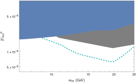
(a)

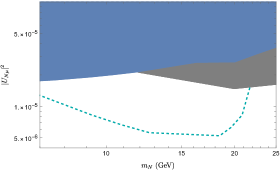
(b)

Figure 17: Potential sensitivity reach of the HL-LHC for $N\chi\bar{\chi}$ signals for the electron-mixing angle (left) and muon-mixing angle (right). The grey regions indicate current exclusion limits from CMS prompt searches in [116], while navy regions are excluded by other collider and beam dump searches. Dashed lines bound the region where 5-$\sigma$ significance can be obtained for the $N\chi\bar{\chi}$ signal over the single-$N$ signal, with $\mathcal{L}=3000\textrm{ fb}^{-1}$.

5.2.2 Region B: Displaced

As in the prompt region, for the displaced region we apply the same methods as for our single-$N$ study (Section 5.1.2) to the $N\chi\bar{\chi}$ signal. We expect this search to be most sensitive in the same parameter region as for the single-$N$ search, since for $m_{N}$ below this range, the $N$ is too long-lived to decay in the tracker region, while for $m_{N}$ above this range, the mixing angle must be very small to allow $m_{N}$ to decay displaced, which results in too low a cross section.

As with the prompt analysis, we look for cuts in the $M_{3\ell}$ and MET variables to maximize the significance of the $N\chi\bar{\chi}$ component in the signal for each parameter point. We find that for the full HL-LHC luminosity (${\mathcal{L}}=3~{}{\rm ab}^{-1}$), even with optimized MET and $M_{3\ell}$ cuts, the region in which $5\sigma$ significance can be obtained for the $N\chi\bar{\chi}$ events over single-$N$ events is entirely contained within the region already excluded by the ATLAS single-$N$ displaced search; therefore no contour for future displaced search projections for the $N\chi\bar{\chi}$ signal is shown. Moreover, CMS’s recent displaced single-$N$ search Ref. [120] places even stronger limits than ATLAS’s search (the ATLAS exclusion region is entirely contained within CMS’s). A displaced search optimized specifically for the $N\chi\bar{\chi}$ signal could provide more promising results. In Section 5.3 we discuss the possibility of a search looking for fully visible $N$ decays.

5.2.3 Region C: Long-Lived

Note that in the parameter region where MATHUSLA is most sensitive to long-lived $N$’s, the production mechanism is through heavy meson decays (mediated by virtual electroweak bosons). As before, in order to get $N\chi\bar{\chi}$ events, we need to replace the $N$ in the single-$N$ signal by an $N_{2}$, which subsequently decays. This has two important consequences. First, there is a range where $N_{2}$ is heavier than the meson, while $N$ is lighter than the meson. In this range, the $N\chi\bar{\chi}$ signal will be negligible compared to the single-$N$ signal because $N_{2}$ production is kinematically forbidden. Therefore, we only expect MATHUSLA to have the capability to observe an $N\chi\bar{\chi}$ excess over the single-$N$ signal for the lower $m_{N}$ range of its sensitivity to the single-$N$ signal. Secondly, there can exist ranges of parameter space where, due to chirality suppression, the decays of specific mesons to $N_{2}$ are preferred over decays to $N$. In this scenario, the amplitudes for two-body decays of the meson into $N+\ell$ or $N_{2}+\ell$ are enhanced by $m_{N}$ or $m_{N_{2}}$ respectively [123, 124]. Hence there are corners of parameter space where the $N\chi\bar{\chi}$ signal may be enhanced over the single-$N$ signal compared to naive expectations.

We calculate a statistical significance for the $N\chi\bar{\chi}$ excess by counting the total events expected to be seen in MATHUSLA for each point in the parameter space. In Figure 18, the region bounded by the purple dashed curve is where the $N\chi\bar{\chi}$ excess has a statistical significance of 5$\sigma$ or above (and where the single-$N$ signal is not excluded by existing constraints). In comparison, the orange line represents the projected reach for the single-$N$ signal at the full HL-LHC luminosity of 3 ab^-1.

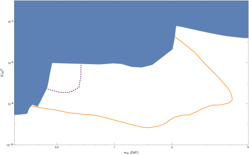
Figure 18: Projected reach for HNL decays in MATHUSLA (orange contour) at $\mathcal{L}=3\textrm{ ab}^{-1}$. The dashed purple curve bounds the region where an $N\chi\bar{\chi}$ excess of events can be observed with $5\sigma$ or greater statistical significance. The navy-shade region is excluded by existing collider and beam dump limits on $|U_{Ne}|^{2}$.

5.3 Possibility of Searching for Fully Visible $N$ decays

Until now, we have mainly focused on existing searches and projecting their sensitivity to single-$N$ production and $N\chi\bar{\chi}$ production at high luminosity. These searches are all based on the leptonic decays of $N$. Since the leptonic decay of $N$ contains a neutrino in the final state, the $N$ itself cannot be reconstructed. In this section, we want to consider a different type of search based on the fully visible decay channel $N\to\ell^{\pm}q\bar{q}^{\prime}$. Since the $N\chi\bar{\chi}$ signal is always subdominant, we should expect that $N$ will be discovered first in the single-$N$ channel, probably in one of the fully leptonic channels. But once this happens, more challenging final states also become very interesting and may yield better sensitivity to subdominant processes such as $N\chi\bar{\chi}$. If $m_{N}$ can be fitted after the discovery of $N$ in a traditional channel, it will be an important variable in reducing the backgrounds in the fully visible search channel.

Fortunately, due to the Majorana nature of $N$, the two leptons in the fully visible channel (one produced in association with $N$ and the other arising from its decay) can be the same sign (and they will always have the same flavor in our model). This helps eliminate the largest SM backgrounds such as $Z+$jets. Unfortunately, the remaining background is expected to be dominated by fakes and detector effects such as lepton charge mismeasurement, and their reliable estimation is beyond the scope of this paper. In this section, we will simply compare the $N\chi\bar{\chi}$ signal to the single-$N$ signal in the fully visible channel and study the statistical significance of the excess. Projections for a dedicated search in this channel should be conducted by experimental collaborations. In other words, below we simply aim to demonstrate what might be possible if the backgrounds can be sufficiently reduced.

The fully visible decay channel of $N$ not only has a higher branching fraction compared to the leptonic one, but it has the very important advantage that the $N$ momentum can be fully reconstructed. As before, we take finite energy resolution into account in the study below by passing all events through Delphes [106]. In order to discriminate between the two signal components, we focus on the variable $m_{N\ell}$, the invariant mass of the $N-\ell$ system, where $\ell$ is the lepton produced in association with the $N$. While for single-$N$ events we expect the distribution of $m_{N\ell}$ to be sharply peaked around $m_{W}$, the distribution for $N\chi\bar{\chi}$ events will be broad and peak at $m_{N\ell}<m_{W}$ due to the DM particles carrying away energy. An example of this for the parameter point $m_{N}=10\textrm{ GeV}$ and $|U_{N\ell}|^{2}=10^{-5}$ is shown in Figure 19.

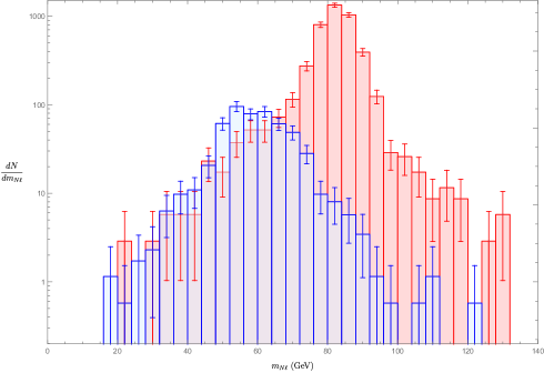
Figure 19: The distribution of $m_{N\ell}$ with $\mathcal{L}=3\textrm{ ab}^{-1}$ for a single-$N$ signal events (red) and $N\chi\bar{\chi}$ events (blue) at the parameter point $m_{N}=10$ GeV and $|U_{N\ell}|^{2}=10^{-5}$. The error bars correspond to statistical uncertainties in our analysis, and they include uncertainties due to the finite size of our Monte Carlo event samples.

Accordingly, we perform a MC study for this final state (a same-sign, same-flavor lepton pair plus jets, $e$ and $\mu$ channels combined) with 3 ab^-1 of luminosity, with only minimal $p_{T}$ requirements for the leptons and $p_{T}>10\textrm{ GeV}$ for jets. We require that two jets and one of the leptons reproduce a particle of mass $m_{N}$ within a tolerance of 20%. We also demand that the invariant mass of the two leptons not be within $15\textrm{ GeV}$ of $m_{Z}$, since a $Z$-veto will almost certainly be used in a dedicated search to reduce the $Z+$jets background with the charge of one lepton misidentified. By performing a shape analysis of the $m_{N\ell}$ distribution, we evaluate the statistical significance of the $\sigma_{N\chi\bar{\chi}}$ excess. Our results for the two combined channels assuming $U_{Ne}=U_{N\mu}$ are shown in Figure 20. This search can reach as far as $|U_{N\ell}|^{2}\sim 10^{-7}$. Below $m_{N}\lesssim 2\textrm{ GeV}$, $N$ becomes too long-lived to decay consistently in the LHC tracker system, but more sophisticated techniques such as searches for particles decaying in the muon trackers could in principle extend sensitivity beyond this limit. For $N$ masses above 30 GeV, the $N_{2}$ becomes too heavy to be produced via Drell-Yan processes.

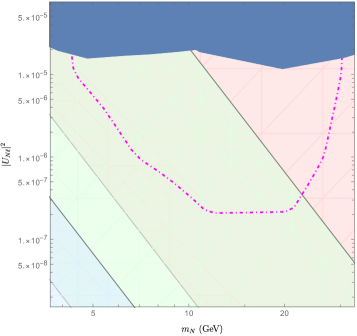
Figure 20: Above the magenta dot-dashed curve, a shape analysis of $m_{N\ell}$ in the visible $N$ decay channel can yield a 5$\sigma$ statistical significance for the $N\chi\bar{\chi}$ signal component in the absence of SM backgrounds. The navy-shaded region is currently excluded by searches for single-$N$ events. The regions shaded pink, green, and blue correspond to parts of parameter space optimally sensitive to prompt, displaced, and long-lived particle searches respectively.

In Figure 21 we show our results for the $\mu$- and $e$-channels separately. Focusing first on the reach of collider searches independently from other constraints, it is easy to see that as the LHC continues its operation, the reach for the discovery of $N$ will be increased significantly both in the prompt and displaced regions via ongoing HNL searches, as well as in the long-lived region if the MATHUSLA experiment. Furthermore, a discovery of $N$ in the prompt and displaced regions could be followed up with a visible search along the lines we described, providing sensitivity for the associated production of a $\chi$-$\bar{\chi}$ pair, establishing their connection to the neutrino portal. There is a region of parameter space where MATHUSLA would be sensitive to $\chi$-$\bar{\chi}$ production for long-lived $N$ as well.

If $\chi$ constitutes all of DM, then as we saw in the previous section. the indirect detection constraints push the $\chi$ mass to $20\,$GeV and above in the $m_{\chi}>M_{N}/2$ case, which pushes the $N$ mass even higher. While this leaves room for the discovery of $N$ itself at the LHC, it eliminates all but the highest possible mass values for which there is sensitivity to $N\chi$-$\bar{\chi}$ production. As previously mentioned however, if $\chi$ does not constitute all of DM, then the indirect detection constraints are weakened, opening up the part of parameter space where DM production may be detectable.

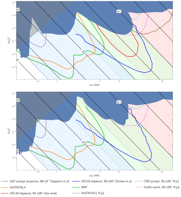
Figure 21: Parameter space of $|U_{N\ell}|^{2}$ plotted against $m_{N}$, with contours of the $N$ lifetime in meters overlaid (diagonal), for the muon mixing angle (above) and electron mixing angle (below). The navy-shaded regions in each plot are excluded by existing collider and beam dump constraints. Solid colored lines represent projected exclusion limits for single-$N$ sensitivity. Dashed contours represent exclusion limits for $N\chi\bar{\chi}$ sensitivity. The dot-dashed magenta contour is our optimistic $N\chi\bar{\chi}$ sensitivity for a visible collider search. In the gray-shaded region, the lifetime of $N$ in our model varies by more than a factor of 2 from that of a generic HNL due to the presence of the $N\to 3\nu$ decay channel.

6 Conclusions

We have explored a class of models with a strongly interacting dark sector coupled to the SM via the neutrino portal that can provide an explanation for both the origin of DM and the smallness of neutrino masses. We have studied the phenomenology of this scenario by modeling it in a warped extra dimensional framework. Within this higher-dimensional construction, we have discussed how neutrino masses can be generated via the inverse seesaw mechanism and we have shown how a stable state in the dark sector can play the role of a DM candidate. We determined the region in the parameter space of the model where the correct DM relic abundance can be obtained through thermal freeze-out, and we have studied the signals of this class of models in direct and indirect detection experiments and in collider searches.

Referring to the state interpolated through the neutrino portal as $N$, and to the DM candidate as $\chi$, the experimental signatures of the model depend strongly on the mass ratio $m_{\chi}/m_{N}$. When this ratio is smaller than $1/2$, $N$ will dominantly decay invisibly, weakening constraints on the model, but also making it challenging to discover. In this scenario, indirect detection is relatively insensitive and collider and beam dump searches that rely on visible decay products have no sensitivity. The main constraints on the model arise from DM self-interactions, bounds on lepton flavor violating processes (since the $N$ mass basis may not align with the flavor basis), direct detection experiments, precision electroweak measurements, and beam dump searches that do not require that $N$ decay in a visible channel. When the mass ratio is larger than $1/2$, the dominant decay of $N$ occurs through the neutrino portal into SM states, and therefore indirect detection experiments and collider searches have sensitivity. The lower bound on $m_{\chi}$ is significantly higher in this case due to constraints from the CMB and from the Fermi experiment. Near-future searches for lepton flavor violation will be able to probe a major part of the allowed parameter space. Future direct detection experiments will also have some level of sensitivity.

When $N$ decays visibly, for the purposes of collider searches, it falls into the category of a heavy neutral lepton (HNL). For HNL searches to have sensitivity, $N$ needs to be light enough to be produced from on-shell $W$-bosons (or even lighter to be produced in the decays of heavy mesons). Therefore, a potential discovery at the LHC is in tension with the existing constraints from indirect detection. The latter can however be weakened if $\chi$ constitutes only part of DM. In that case, as the luminosity of the LHC increases, additional regions in parameter space will be probed by searches looking for prompt as well as displaced decays of $N$, and complementary experiments such as MATHUSLA can probe the very long-lived $N$ region. An additional challenge is posed by discovering not only $N$ itself, but the production of DM particles along with it. We have shown that existing search strategies would not be sensitive to this production channel in regions of parameter space that are not already in tension with existing bounds. However we have proposed an extended search strategy based on the reconstruction of $N$ in a visible decay channel that would have sensitivity in the prompt and displaced $N$ decay regions. An interesting direction for future study would be the sensitivity of future experiments such as a high energy lepton collider to $N$ production channels such as $e^{+}e^{-}\to N\bar{\nu}$ which would not be limited to low $N$ masses as in the case of Drell-Yan production. Such a search may be sensitive to the region of parameter space that is compatible with indirect detection searches even when $\chi$ constitutes all of DM.

References

- [1] A. E. Faraggi and M. Pospelov, “Selfinteracting dark matter from the hidden heterotic string sector,” Astropart. Phys. 16 (2002) 451–461, [hep-ph/0008223].
- [2] A. Soni and Y. Zhang, “Hidden SU(N) Glueball Dark Matter,” Phys. Rev. D 93 no. 11, (2016) 115025, [arXiv:1602.00714].
- [3] Y. Bai and R. J. Hill, “Weakly Interacting Stable Pions,” Phys. Rev. D 82 (2010) 111701, [arXiv:1005.0008].
- [4] S. Bhattacharya, B. Melić, and J. Wudka, “Pionic Dark Matter,” JHEP 02 (2014) 115, [arXiv:1307.2647].
- [5] J. M. Cline, Z. Liu, G. D. Moore, and W. Xue, “Composite strongly interacting dark matter,” Phys. Rev. D 90 no. 1, (2014) 015023, [arXiv:1312.3325].
- [6] Y. Hochberg, E. Kuflik, H. Murayama, T. Volansky, and J. G. Wacker, “Model for Thermal Relic Dark Matter of Strongly Interacting Massive Particles,” Phys. Rev. Lett. 115 no. 2, (2015) 021301, [arXiv:1411.3727].
- [7] V. Beylin, M. Y. Khlopov, V. Kuksa, and N. Volchanskiy, “Hadronic and Hadron-Like Physics of Dark Matter,” Symmetry 11 no. 4, (2019) 587, [arXiv:1904.12013].
- [8] H. M. Hodges, “Mirror baryons as the dark matter,” Phys. Rev. D 47 (1993) 456–459.
- [9] Z. Berezhiani, D. Comelli, and F. L. Villante, “The Early mirror universe: Inflation, baryogenesis, nucleosynthesis and dark matter,” Phys. Lett. B 503 (2001) 362–375, [hep-ph/0008105].
- [10] R. Foot, “Mirror matter-type dark matter,” Int. J. Mod. Phys. D 13 (2004) 2161–2192, [astro-ph/0407623].
- [11] J. M. Cline, “Dark atoms and composite dark matter,” SciPost Phys. Lect. Notes 52 (2022) 1, [arXiv:2108.10314].
- [12] L. E. Ibanez, “The Scalar Neutrinos as the Lightest Supersymmetric Particles and Cosmology,” Phys. Lett. B 137 (1984) 160–164.
- [13] J. S. Hagelin, G. L. Kane, and S. Raby, “Perhaps Scalar Neutrinos Are the Lightest Supersymmetric Partners,” Nucl. Phys. B 241 (1984) 638–652.
- [14] L. J. Hall, T. Moroi, and H. Murayama, “Sneutrino cold dark matter with lepton number violation,” Phys. Lett. B 424 (1998) 305–312, [hep-ph/9712515].
- [15] S. Dodelson and L. M. Widrow, “Sterile-neutrinos as dark matter,” Phys. Rev. Lett. 72 (1994) 17–20, [hep-ph/9303287].
- [16] X.-D. Shi and G. M. Fuller, “A New dark matter candidate: Nonthermal sterile neutrinos,” Phys. Rev. Lett. 82 (1999) 2832–2835, [astro-ph/9810076].
- [17] K. Abazajian, G. M. Fuller, and M. Patel, “Sterile neutrino hot, warm, and cold dark matter,” Phys. Rev. D 64 (2001) 023501, [astro-ph/0101524].
- [18] E. Ma, “Verifiable radiative seesaw mechanism of neutrino mass and dark matter,” Phys. Rev. D 73 (2006) 077301, [hep-ph/0601225].
- [19] C. Boehm, Y. Farzan, T. Hambye, S. Palomares-Ruiz, and S. Pascoli, “Is it possible to explain neutrino masses with scalar dark matter?,” Phys. Rev. D 77 (2008) 043516, [hep-ph/0612228].
- [20] T. Hambye, F. S. Ling, L. Lopez Honorez, and J. Rocher, “Scalar Multiplet Dark Matter,” JHEP 07 (2009) 090, [arXiv:0903.4010]. [Erratum: JHEP 05, 066 (2010)].
- [21] M. Escudero, N. Rius, and V. Sanz, “Sterile Neutrino portal to Dark Matter II: Exact Dark symmetry,” Eur. Phys. J. C 77 no. 6, (2017) 397, [arXiv:1607.02373].
- [22] B. Batell, T. Han, D. McKeen, and B. Shams Es Haghi, “Thermal Dark Matter Through the Dirac Neutrino Portal,” Phys. Rev. D 97 no. 7, (2018) 075016, [arXiv:1709.07001].
- [23] J. M. Lamprea, E. Peinado, S. Smolenski, and J. Wudka, “Self-interacting neutrino portal dark matter,” Phys. Rev. D 103 no. 1, (2021) 015017, [arXiv:1906.02340].
- [24] R. N. Mohapatra and J. W. F. Valle, “Neutrino Mass and Baryon Number Nonconservation in Superstring Models,” Phys. Rev. D 34 (1986) 1642.
- [25] R. N. Mohapatra, “Mechanism for Understanding Small Neutrino Mass in Superstring Theories,” Phys. Rev. Lett. 56 (1986) 561–563.
- [26] N. Arkani-Hamed and Y. Grossman, “Light active and sterile neutrinos from compositeness,” Phys. Lett. B 459 (1999) 179–182, [hep-ph/9806223].
- [27] G. von Gersdorff and M. Quiros, “Conformal Neutrinos: an Alternative to the See-saw Mechanism,” Phys. Lett. B 678 (2009) 317–321, [arXiv:0901.0006].
- [28] Y. Grossman and D. J. Robinson, “Composite Dirac Neutrinos,” JHEP 01 (2011) 132, [arXiv:1009.2781].
- [29] T. Okui, “Searching for composite neutrinos in the cosmic microwave background,” JHEP 09 (2005) 017, [hep-ph/0405083].
- [30] D. J. Robinson and Y. Tsai, “KeV Warm Dark Matter and Composite Neutrinos,” JHEP 08 (2012) 161, [arXiv:1205.0569].
- [31] D. J. Robinson and Y. Tsai, “Dynamical framework for KeV Dirac neutrino warm dark matter,” Phys. Rev. D 90 no. 4, (2014) 045030, [arXiv:1404.7118].
- [32] R. S. Hundi and S. Roy, “Constraints on composite Dirac neutrinos from observations of galaxy clusters,” Phys. Lett. B 702 (2011) 228–234, [arXiv:1105.0291].
- [33] H. Davoudiasl, P. P. Giardino, E. T. Neil, and E. Rinaldi, “Unified Scenario for Composite Right-Handed Neutrinos and Dark Matter,” Phys. Rev. D 96 no. 11, (2017) 115003, [arXiv:1709.01082].
- [34] Y. Grossman and Y. Tsai, “Leptogenesis with Composite Neutrinos,” JHEP 12 (2008) 016, [arXiv:0811.0871].
- [35] Z. Chacko, P. J. Fox, R. Harnik, and Z. Liu, “Neutrino Masses from Low Scale Partial Compositeness,” JHEP 03 (2021) 112, [arXiv:2012.01443].
- [36] J. M. Maldacena, “The Large N limit of superconformal field theories and supergravity,” Int. J. Theor. Phys. 38 (1999) 1113–1133, [hep-th/9711200].
- [37] S. Gubser, I. R. Klebanov, and A. M. Polyakov, “Gauge theory correlators from noncritical string theory,” Phys. Lett. B 428 (1998) 105–114, [hep-th/9802109].
- [38] E. Witten, “Anti-de Sitter space and holography,” Adv. Theor. Math. Phys. 2 (1998) 253–291, [hep-th/9802150].
- [39] I. R. Klebanov and E. Witten, “AdS / CFT correspondence and symmetry breaking,” Nucl. Phys. B 556 (1999) 89–114, [hep-th/9905104].
- [40] L. Randall and R. Sundrum, “A Large mass hierarchy from a small extra dimension,” Phys. Rev. Lett. 83 (1999) 3370–3373, [hep-ph/9905221].
- [41] Y. Grossman and M. Neubert, “Neutrino masses and mixings in nonfactorizable geometry,” Phys. Lett. B 474 (2000) 361–371, [hep-ph/9912408].
- [42] S. J. Huber and Q. Shafi, “Majorana neutrinos in a warped 5-D standard model,” Phys. Lett. B 544 (2002) 295–306, [hep-ph/0205327].
- [43] S. J. Huber and Q. Shafi, “Seesaw mechanism in warped geometry,” Phys. Lett. B 583 (2004) 293–303, [hep-ph/0309252].
- [44] K. Agashe, S. Hong, and L. Vecchi, “Warped seesaw mechanism is physically inverted,” Phys. Rev. D 94 no. 1, (2016) 013001, [arXiv:1512.06742].
- [45] T. Gherghetta, “Dirac neutrino masses with Planck scale lepton number violation,” Phys. Rev. Lett. 92 (2004) 161601, [hep-ph/0312392].
- [46] K. Agashe and G. Servant, “Warped unification, proton stability and dark matter,” Phys. Rev. Lett. 93 (2004) 231805, [hep-ph/0403143].
- [47] K. Agashe and G. Servant, “Baryon number in warped GUTs: Model building and (dark matter related) phenomenology,” JCAP 02 (2005) 002, [hep-ph/0411254].
- [48] G. Belanger, A. Pukhov, and G. Servant, “Dirac Neutrino Dark Matter,” JCAP 01 (2008) 009, [arXiv:0706.0526].
- [49] G. Panico, E. Ponton, J. Santiago, and M. Serone, “Dark Matter and Electroweak Symmetry Breaking in Models with Warped Extra Dimensions,” Phys. Rev. D 77 (2008) 115012, [arXiv:0801.1645].
- [50] K. L. McDonald, “Light Neutrinos from a Mini-Seesaw Mechanism in Warped Space,” Phys. Lett. B696 (2011) 266–272, [arXiv:1010.2659].
- [51] B. Gripaios, “Neutrinos in a Sterile Throat,” Nucl. Phys. B 768 (2007) 157–176, [hep-ph/0611218]. [Erratum: Nucl.Phys.B 830, 390–390 (2010)].
- [52] LUX-ZEPLIN Collaboration, D. S. Akerib et al., “Projected WIMP sensitivity of the LUX-ZEPLIN dark matter experiment,” Phys. Rev. D 101 no. 5, (2020) 052002, [arXiv:1802.06039].
- [53] XENON Collaboration, E. Aprile et al., “Physics reach of the XENON1T dark matter experiment,” JCAP 04 (2016) 027, [arXiv:1512.07501].
- [54] S. Tulin and H.-B. Yu, “Dark Matter Self-interactions and Small Scale Structure,” Phys. Rept. 730 (2018) 1–57, [arXiv:1705.02358].
- [55] P.-W. Chang, I. Esteban, J. F. Beacom, T. A. Thompson, and C. M. Hirata, “Towards Powerful Probes of Neutrino Self-Interactions in Supernovae,” arXiv:2206.12426.
- [56] Super-Kamiokande Collaboration, Y. Fukuda et al., “The Super-Kamiokande detector,” Nucl. Instrum. Meth. A 501 (2003) 418–462.
- [57] K. Abe et al., “Letter of Intent: The Hyper-Kamiokande Experiment — Detector Design and Physics Potential —,” arXiv:1109.3262.
- [58] DUNE Collaboration, B. Abi et al., “The DUNE Far Detector Interim Design Report Volume 1: Physics, Technology and Strategies,” arXiv:1807.10334.
- [59] DUNE Collaboration, B. Abi et al., “The DUNE Far Detector Interim Design Report, Volume 2: Single-Phase Module,” arXiv:1807.10327.
- [60] DUNE Collaboration, B. Abi et al., “The DUNE Far Detector Interim Design Report, Volume 3: Dual-Phase Module,” arXiv:1807.10340.
- [61] JUNO Collaboration, F. An et al., “Neutrino Physics with JUNO,” J. Phys. G 43 no. 3, (2016) 030401, [arXiv:1507.05613].
- [62] LUX-ZEPLIN Collaboration, J. Aalbers et al., “First Dark Matter Search Results from the LUX-ZEPLIN (LZ) Experiment,” arXiv:2207.03764.
- [63] D. Curtin et al., “Long-Lived Particles at the Energy Frontier: The MATHUSLA Physics Case,” Rept. Prog. Phys. 82 no. 11, (2019) 116201, [arXiv:1806.07396].
- [64] N. Arkani-Hamed, M. Porrati, and L. Randall, “Holography and phenomenology,” JHEP 08 (2001) 017, [hep-th/0012148].
- [65] R. Rattazzi and A. Zaffaroni, “Comments on the holographic picture of the Randall-Sundrum model,” JHEP 04 (2001) 021, [hep-th/0012248].
- [66] R. Contino and A. Pomarol, “Holography for fermions,” JHEP 11 (2004) 058, [hep-th/0406257].
- [67] G. Cacciapaglia, G. Marandella, and J. Terning, “Dimensions of Supersymmetric Operators from AdS/CFT,” JHEP 06 (2009) 027, [arXiv:0802.2946].
- [68] N. Desai, C. Kilic, Y.-P. Yang, and T. Youn, “Suppressed flavor violation in Lepton Flavored Dark Matter from an extra dimension,” Phys. Rev. D 101 (2020) 075043, [arXiv:2001.00720].
- [69] H. Davoudiasl, G. Perez, and A. Soni, “The Little Randall-Sundrum Model at the Large Hadron Collider,” Phys. Lett. B 665 (2008) 67–71, [arXiv:0802.0203].
- [70] D. P. George and K. L. McDonald, “Gravity on a Little Warped Space,” Phys. Rev. D 84 (2011) 064007, [arXiv:1107.0755].
- [71] R. T. D’Agnolo and J. T. Ruderman, “Light Dark Matter from Forbidden Channels,” Phys. Rev. Lett. 115 no. 6, (2015) 061301, [arXiv:1505.07107].
- [72] G. Belanger, A. Mjallal, and A. Pukhov, “Recasting direct detection limits within micrOMEGAs and implication for non-standard Dark Matter scenarios,” Eur. Phys. J. C 81 no. 3, (2021) 239, [arXiv:2003.08621].
- [73] Planck Collaboration, N. Aghanim et al., “Planck 2018 results. VI. Cosmological parameters,” Astron. Astrophys. 641 (2020) A6, [arXiv:1807.06209]. [Erratum: Astron.Astrophys. 652, C4 (2021)].
- [74] H. H. Patel, “Package-X 2.0: A Mathematica package for the analytic calculation of one-loop integrals,” Comput. Phys. Commun. 218 (2017) 66–70, [arXiv:1612.00009].
- [75] T. R. Slatyer, “Indirect dark matter signatures in the cosmic dark ages. I. Generalizing the bound on s-wave dark matter annihilation from Planck results,” Phys. Rev. D 93 no. 2, (2016) 023527, [arXiv:1506.03811].
- [76] T. Sjöstrand, S. Ask, J. R. Christiansen, R. Corke, N. Desai, P. Ilten, S. Mrenna, S. Prestel, C. O. Rasmussen, and P. Z. Skands, “An introduction to PYTHIA 8.2,” Comput. Phys. Commun. 191 (2015) 159–177, [arXiv:1410.3012].
- [77] W. L. K. Wu, J. Errard, C. Dvorkin, C. L. Kuo, A. T. Lee, P. McDonald, A. Slosar, and O. Zahn, “A Guide to Designing Future Ground-based Cosmic Microwave Background Experiments,” Astrophys. J. 788 (2014) 138, [arXiv:1402.4108].
- [78] Fermi-LAT Collaboration, S. Abdollahi et al., “ Large Area Telescope Fourth Source Catalog,” Astrophys. J. Suppl. 247 no. 1, (2020) 33, [arXiv:1902.10045].
- [79] K. N. Abazajian, S. Horiuchi, M. Kaplinghat, R. E. Keeley, and O. Macias, “Strong constraints on thermal relic dark matter from Fermi-LAT observations of the Galactic Center,” Phys. Rev. D 102 no. 4, (2020) 043012, [arXiv:2003.10416].
- [80] J. F. Navarro, C. S. Frenk, and S. D. M. White, “The Structure of cold dark matter halos,” Astrophys. J. 462 (1996) 563–575, [astro-ph/9508025].
- [81] J. I. Read, O. Agertz, and M. L. M. Collins, “Dark matter cores all the way down,” Mon. Not. Roy. Astron. Soc. 459 no. 3, (2016) 2573–2590, [arXiv:1508.04143].
- [82] Fermi-LAT Collaboration, M. Ackermann et al., “Searching for Dark Matter Annihilation from Milky Way Dwarf Spheroidal Galaxies with Six Years of Fermi Large Area Telescope Data,” Phys. Rev. Lett. 115 no. 23, (2015) 231301, [arXiv:1503.02641].
- [83] Fermi-LAT, DES Collaboration, A. Albert et al., “Searching for Dark Matter Annihilation in Recently Discovered Milky Way Satellites with Fermi-LAT,” Astrophys. J. 834 no. 2, (2017) 110, [arXiv:1611.03184].
- [84] A. Geringer-Sameth, S. M. Koushiappas, and M. Walker, “Dwarf galaxy annihilation and decay emission profiles for dark matter experiments,” Astrophys. J. 801 no. 2, (2015) 74, [arXiv:1408.0002].
- [85] Super-Kamiokande Collaboration, K. Abe et al., “Indirect search for dark matter from the Galactic Center and halo with the Super-Kamiokande detector,” Phys. Rev. D 102 no. 7, (2020) 072002, [arXiv:2005.05109].
- [86] IceCube Collaboration, R. Abbasi et al., “Indirect search for dark matter in the Galactic Centre with IceCube,” in 37th International Cosmic Ray Conference. 7, 2021. arXiv:2107.11224.
- [87] A. Albert et al., “Results from the search for dark matter in the Milky Way with 9 years of data of the ANTARES neutrino telescope,” Phys. Lett. B 769 (2017) 249–254, [arXiv:1612.04595]. [Erratum: Phys.Lett.B 796, 253–255 (2019)].
- [88] A. Olivares-Del Campo, C. Bœhm, S. Palomares-Ruiz, and S. Pascoli, “Dark matter-neutrino interactions through the lens of their cosmological implications,” Phys. Rev. D 97 no. 7, (2018) 075039, [arXiv:1711.05283].
- [89] N. Klop and S. Ando, “Constraints on MeV dark matter using neutrino detectors and their implication for the 21-cm results,” Phys. Rev. D 98 no. 10, (2018) 103004, [arXiv:1809.00671].
- [90] C. A. Argüelles, A. Diaz, A. Kheirandish, A. Olivares-Del-Campo, I. Safa, and A. C. Vincent, “Dark matter annihilation to neutrinos,” Rev. Mod. Phys. 93 no. 3, (2021) 035007, [arXiv:1912.09486].
- [91] N. F. Bell, M. J. Dolan, and S. Robles, “Searching for Sub-GeV Dark Matter in the Galactic Centre using Hyper-Kamiokande,” JCAP 09 (2020) 019, [arXiv:2005.01950].
- [92] S. Abe et al., “Limits on astrophysical antineutrinos with the KamLAND experiment,” arXiv:2108.08527.
- [93] Hyper-Kamiokande Collaboration, K. Abe et al., “Hyper-Kamiokande Design Report,” arXiv:1805.04163.
- [94] DUNE Collaboration, R. Acciarri et al., “Long-Baseline Neutrino Facility (LBNF) and Deep Underground Neutrino Experiment (DUNE): Conceptual Design Report, Volume 2: The Physics Program for DUNE at LBNF,” arXiv:1512.06148.
- [95] A. Olivares-Del Campo, S. Palomares-Ruiz, and S. Pascoli, “Implications of a Dark Matter-Neutrino Coupling at Hyper-Kamiokande,” in 53rd Rencontres de Moriond on Electroweak Interactions and Unified Theories, pp. 441–444. 2018. arXiv:1805.09830.
- [96] C. Boehm, M. J. Dolan, and C. McCabe, “A Lower Bound on the Mass of Cold Thermal Dark Matter from Planck,” JCAP 08 (2013) 041, [arXiv:1303.6270].
- [97] K. M. Nollett and G. Steigman, “BBN And The CMB Constrain Neutrino Coupled Light WIMPs,” Phys. Rev. D 91 no. 8, (2015) 083505, [arXiv:1411.6005].
- [98] M. Escudero, “Neutrino decoupling beyond the Standard Model: CMB constraints on the Dark Matter mass with a fast and precise evaluation,” JCAP 02 (2019) 007, [arXiv:1812.05605].
- [99] MEG Collaboration, A. M. Baldini et al., “Search for the lepton flavour violating decay with the full dataset of the MEG experiment,” Eur. Phys. J. C 76 no. 8, (2016) 434, [arXiv:1605.05081].
- [100] SINDRUM II Collaboration, W. H. Bertl et al., “A Search for muon to electron conversion in muonic gold,” Eur. Phys. J. C 47 (2006) 337–346.
- [101] Mu2e Collaboration, L. Bartoszek et al., “Mu2e Technical Design Report,” arXiv:1501.05241.
- [102] COMET Collaboration, R. Abramishvili et al., “COMET Phase-I Technical Design Report,” PTEP 2020 no. 3, (2020) 033C01, [arXiv:1812.09018].
- [103] A. de Gouvêa and A. Kobach, “Global Constraints on a Heavy Neutrino,” Phys. Rev. D 93 no. 3, (2016) 033005, [arXiv:1511.00683].
- [104] A. M. Abdullahi et al., “The present and future status of heavy neutral leptons,” J. Phys. G 50 no. 2, (2023) 020501, [arXiv:2203.08039].
- [105] J. Alwall, R. Frederix, S. Frixione, V. Hirschi, F. Maltoni, O. Mattelaer, H. S. Shao, T. Stelzer, P. Torrielli, and M. Zaro, “The automated computation of tree-level and next-to-leading order differential cross sections, and their matching to parton shower simulations,” JHEP 07 (2014) 079, [arXiv:1405.0301].
- [106] DELPHES 3 Collaboration, J. de Favereau, C. Delaere, P. Demin, A. Giammanco, V. Lemaître, A. Mertens, and M. Selvaggi, “DELPHES 3, A modular framework for fast simulation of a generic collider experiment,” JHEP 02 (2014) 057, [arXiv:1307.6346].
- [107] M. Daum, B. Jost, R. M. Marshall, R. C. Minehart, W. A. Stephens, and K. O. H. Ziock, “Search for Admixtures of Massive Neutrinos in the Decay Neutrino,” Phys. Rev. D 36 (1987) 2624.
- [108] PIENU Collaboration, A. Aguilar-Arevalo et al., “Search for heavy neutrinos in decay,” Phys. Lett. B 798 (2019) 134980, [arXiv:1904.03269].
- [109] R. S. Hayano et al., “HEAVY NEUTRINO SEARCH USING K(mu2) DECAY,” Phys. Rev. Lett. 49 (1982) 1305.
- [110] BNL-E949 Collaboration, A. V. Artamonov et al., “Study of the decay in the momentum region MeV/c,” Phys. Rev. D 79 (2009) 092004, [arXiv:0903.0030].
- [111] T2K Collaboration, K. Abe et al., “Search for heavy neutrinos with the T2K near detector ND280,” Phys. Rev. D 100 no. 5, (2019) 052006, [arXiv:1902.07598].
- [112] G. Bernardi et al., “Search for Neutrino Decay,” Phys. Lett. B 166 (1986) 479–483.
- [113] G. Bernardi et al., “FURTHER LIMITS ON HEAVY NEUTRINO COUPLINGS,” Phys. Lett. B 203 (1988) 332–334.
- [114] NuTeV, E815 Collaboration, A. Vaitaitis et al., “Search for neutral heavy leptons in a high-energy neutrino beam,” Phys. Rev. Lett. 83 (1999) 4943–4946, [hep-ex/9908011].
- [115] DELPHI Collaboration, P. Abreu et al., “Search for neutral heavy leptons produced in Z decays,” Z. Phys. C 74 (1997) 57–71. [Erratum: Z.Phys.C 75, 580 (1997)].
- [116] CMS Collaboration, A. M. Sirunyan et al., “Search for heavy neutral leptons in events with three charged leptons in proton-proton collisions at 13 TeV,” Phys. Rev. Lett. 120 no. 22, (2018) 221801, [arXiv:1802.02965].
- [117] ATLAS Collaboration, G. Aad et al., “Search for heavy neutral leptons in decays of bosons produced in 13 TeV collisions using prompt and displaced signatures with the ATLAS detector,” JHEP 10 (2019) 265, [arXiv:1905.09787].
- [118] A. Das, P. S. B. Dev, and R. N. Mohapatra, “Same Sign versus Opposite Sign Dileptons as a Probe of Low Scale Seesaw Mechanisms,” Phys. Rev. D 97 no. 1, (2018) 015018, [arXiv:1709.06553].
- [119] E. Izaguirre and B. Shuve, “Multilepton and Lepton Jet Probes of Sub-Weak-Scale Right-Handed Neutrinos,” Phys. Rev. D 91 no. 9, (2015) 093010, [arXiv:1504.02470].
- [120] CMS Collaboration, A. Tumasyan et al., “Search for long-lived heavy neutral leptons with displaced vertices in proton-proton collisions at =13 TeV,” arXiv:2201.05578.
- [121] ATLAS Collaboration, “Search for heavy neutral leptons in decays of bosons using a dilepton displaced vertex in TeV collisions with the ATLAS detector,” arXiv:2204.11988.
- [122] M. Drewes and J. Hajer, “Heavy Neutrinos in displaced vertex searches at the LHC and HL-LHC,” JHEP 02 (2020) 070, [arXiv:1903.06100].
- [123] F. Kling and S. Trojanowski, “Heavy Neutral Leptons at FASER,” Phys. Rev. D 97 no. 9, (2018) 095016, [arXiv:1801.08947].
- [124] K. Bondarenko, A. Boyarsky, D. Gorbunov, and O. Ruchayskiy, “Phenomenology of GeV-scale Heavy Neutral Leptons,” JHEP 11 (2018) 032, [arXiv:1805.08567].