Energy risk analysis with Dynamic Amplitude Estimation and Piecewise Approximate Quantum Compiling

Abstract

We generalize the Approximate Quantum Compiling algorithm into a new method for CNOT-depth reduction, which is apt to process wide target quantum circuits. Combining this method with state-of-the-art techniques for error mitigation and circuit compiling, we present a 10-qubit experimental demonstration of Iterative Amplitude Estimation on a quantum computer. The target application is the derivation of the Expected Value of contract portfolios in the energy industry.

In parallel, we also introduce a new variant of the Quantum Amplitude Estimation algorithm which we call Dynamic Amplitude Estimation, as it is based on the dynamic circuit capability of quantum devices. The algorithm achieves a reduction in the circuit width in the order of the binary precision compared to the typical implementation of Quantum Amplitude Estimation, while simultaneously decreasing the number of quantum-classical iterations (again in the order of the binary precision) compared to the Iterative Amplitude Estimation. The calculation of the Expected Value, VaR and CVaR of contract portfolios on quantum hardware provides a proof of principle of the new algorithm.

1 Introduction

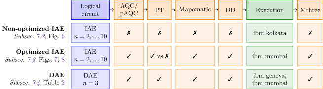
Figure 1: The first row describes the workflow for the production and execution of the quantum circuits used for our estimation. Specifically, the first blue box represents the generation of the logical circuits, whose general method is described in Sec. 4. The green box represents the circuit execution on quantum hardware. The orange boxes represent error mitigation and circuit optimization techniques that reduce the effect of hardware noise: Pauli Twirling (PT), mapomatic, Dynamical Decoupling (DD) and mthree are state-of-the-art techniques described in Subsec. 5.1; Approximate Quantum Compiling (AQC) is presented in Subsec. 5.2, and extended into the new variant of piecewice AQC (pAQC) in Subsec. 5.3. The other lines of the diagram represent the core experiments of the paper. In the ‘logical circuit’ column, we indicate whether Iterative Amplitude Estimation (IAE) or the new Dynamic Amplitude Estimation (DAE) is employed, and the number $n$ of qubits in the input distribution. In the orange columns, we indicate which optimization techniques were used: pAQC is employed in lieu of AQC for $n\geq 8$. Finally, in the execution column we provide the name of the IBM Quantum backend.

The computation of risk measures can be made more time-efficient by resorting to quantum computers, and specifically to the Quantum Amplitude Estimation (QAE) algorithm, but current noisy quantum hardware limits short-term possibilities of real-world applications. We demonstrate three novel contributions in this work. First, we propose a variant of the Approximate Quantum Compiling algorithm (AQC), called Piecewise Approximate Quantum Compiling (pAQC). Like the original AQC, our method is designed to approximate circuits in order to reduce their depth, but the novel variant is more suited for deep circuits. Second, we provide a 10-qubit experimental demonstration of amplitude estimation in quantum hardware, using the Iterative Amplitude Estimation (IAE) in combination with state-of-the art error mitigation and circuit optimization techniques as well as the newly introduced pAQC. We showcase the execution of a 10-qubit amplitude estimation circuit on a quantum computer. Finally, we introduce the Dynamic Amplitude Estimation (DAE), an upgraded version of QAE, leveraging on the dynamic circuit capability recently introduced on IBM Quantum devices [1], thus reducing the circuit width and the number of quantum-classical iterations, in comparison with the previously known equivalent techniques.

Our target application is the calculation of statistical quantities like the Expectation, VaR, and CVaR of the delta gross margin, namely the random variable representing the difference between the forecasted value of a contract portfolio, and its stochastic economic outcome. A faster calculation of such metrics would lead to a real-time planning and decision making, finer risk diversification, as well as more frequent risk assessments for the negotiation of hedging contracts, with radical impacts on risk management in the industry sector. To compute the above risk statistics we use one of the fundamental quantum algorithms called QAE, which achieves a quadratic speedup over classical Monte Carlo (MC) simulation, e.g. in financial services for the purpose of option pricing[2, 3] and risk analysis [4, 5, 6, 7]. The canonical version of QAE is a combination of Quantum Phase Estimation (QPE) [8] and Grover’s Algorithm [9]. The size of the QAE-circuit grows rapidly with the size of encoded probability distribution and the expected accuracy of the result, therefore it needs a large amount of quantum resources for the implementation. Aiming to reduce the required resources, several QAE variants have been introduced in literature, in which QPE is replaced by ad-hoc classical workloads. Early attempts showed either lack of rigorous proof [10, 11], or high constants rendering the algorithm unsuitable for practical applications [12]. The latest developments include Iterative Amplitude Estimation (IAE) [13] and ChebQAE [14], which have both a rigorous proof for the quadratic speed-up (up to a multiplicative $\log(\log(\epsilon^{-1}))$ factor) and much improved constants.

The outline of the article is as follows. Sec 2 contains a summary of our results. In Sec. 3, we begin with an overview of the energy contract risk analysis and the relevant risk measures. In the following Sec. 4, we summarize the workflow, main steps, and the mathematical preliminaries for QAE-inspired risk analysis. In the next Sec. 6, we introduce the novel Dynamic Amplitude Estimation. In Sec. 7, we compute the statistics of the random variable, first using the qasm simulator and then using the quantum computer, with QAE and DAE. The circuit is altered to reduce depth and optimize for the quantum hardware, via multiple techniques: optimal qubit mapping, dynamical decoupling with mapomatic, error mitigation with mthree, Pauli Twirling, and approximate quantum compiler (AQC). Specifically we propose a variant of AQC that operates on wide circuits, the pAQC. In Sec. 8, we highlight some important points of our development and the advantages over its non-dynamical counterparts. Finally, in Sec. 9 we offer some concluding remarks.

Fig. 1 shows how the different error mitigation and circuit optimization techniques combine with IAE and DAE in the experiments.

2 Result summary

This section summarizes our three main contributions.

Piecewise Approximate Quantum Compiling.

Current hardware capabilities constrain the maximal depth of executable circuits, before the noise prevails. Therefore, approximating a circuit with an alternate one having lower depth, proves to be extremely beneficial. Approximate Quantum Compiling (AQC) [15] provides very good results, but unfortunately suffers from a barren plateau effect on wide circuits, and cannot be employed beyond a threshold of $7$ or $8$ qubits, in our experience. Consequently, we contribute with a variant that we call piecewise AQC (pAQC), designed for wide circuits.

A 10-qubit demonstration with IAE, noise mitigation and circuit approximation.

Literature lacks demonstrations of QAE and related techniques beyond very few qubits on quantum computer, with the exception of Ref. [7] that unfortunately does not give details on the effect of errors over estimations. By combining state-of-the-art capabilities in error mitigation and circuit approximation [16, 17, 18, 19], we are able to estimate the Expectation through circuits up to $7$ data qubits.Additionally, by resorting to pAQC, we estimate the Expectation of distributions up to $10$ qubits, with similar error rates. This achievement is far beyond any witnessed result, at the best of the authors’ knowledge.

Dynamic Amplitude Estimation.

The quantum-classical iterative methods, including IAE used above, require multiple subsequent hardware calls, and preclude the possibility to generate all circuits in a single preprocessing phase, thus adding communication overhead, depth unpredictability and warm-start complexities. At the same time, a recent hardware capability, namely dynamic circuits, offers new levers for circuit depth optimization. Correspondingly, a variant of QPE (here called DPE) was developed to reduce the number of qubits, and therefore the gate error propagation, of the original QPE [20]. In this work, we introduce the Dynamic Amplitude Estimation (DAE) in which the qubit-intensive form of original QPE is replaced by a phase estimation circuit that exploits dynamic circuits. The DAE algorithm, compared to QAE, reduces the required number of qubits (from $m$ to 1, for $m$ significant bits), and thus the gate error propagation. Additionally, re-using the same qubit for all measurements implies increased consistency in readout and CNOT errors [21]. Compared to iterative methods such as IAE, DAE reduces the required number of quantum-classical iterations from $\mathcal{O}(m)$ to $1$, allowing for contemporary submission of all jobs. These facts lower the bar to apply QAE in practice. At the same time, DAE has a rigorous proof, which is a mandatory requirement in regulated environments.

The techniques introduced here are relevant beyond the context of energy risk analysis. Indeed, pAQC is beneficial for the reduction of the depth of virtually any circuit. Similarly, DAE is applicable to all fields where QAE methods are employed: primarily for Monte Carlo Integration [22] with implications in finance [2, 4] and physics [23, 24], as well as for optimization [25] and machine learning [26, 27].

3 Energy portfolio risk analysis

In the gas industry, standard contracts for private or industrial customers normally entail fixed unitary prices, and do not include any volume constraints. On the other side, the gas demand of households or heating has a strong dependency on gas volumes and weather variables, typically the temperature, that in turn implies variations of prices in the gas trade market. In other words, the gas supplier takes the risk of volume (and price) deviations from the projected load profile of the customer.

As a consequence, risk managers compute the fair value and the financial exposure deriving from the entire weather-related portfolio, as well as of the individual contracts it consists of. To this end, they rely on a joint stochastic model for the gas prices and temperatures, and perform extensive and time-consuming Monte Carlo simulations [28] to estimate such statistics. Many classical models and approaches are available in the literature which encompass at the same time the joint temperature-gas evolution, the Monte Carlo simulation and the risk analysis (see for instance Benth and Benth [29, 30], Cucu et al [31], Sabino and Cufaro Petroni [32]).

A key economic value in an energy contract portfolio is the change in gross margin $\Delta GM$, defined as follows. Consider a simplified weather-related portfolio which depends on gas and temperature. These two variables are called underlyings. For simplicity, we can consider three gas European markets, Germany, UK, and Italy, and one temperature location relative to each country, Berlin, London, and Rome, respectively. The portfolio we focus on, only consists of supply contracts, based on which the customer can nominate gas volumes at an agreed sales price, denoted as asp. These contracts are then implicitly temperature dependent: indeed, the customers’ demand is modeled by a volume function ($V(T)$) of the temperature.

In this setting, the delta gross margin is defined as the (unknown random) difference between the net random sales less the random costs at a certain time future time $t$ and the planned, therefore known, sales minus cost at the same future time. Formally, let $i=1,2,3$ be an index over the weather stations, and $j=1,...,365$ an index over the time slices in the horizon. Accordingly, the portfolio consists of three contracts each dependent on its relative weather station. In addition, for simplicity, we assume that each station is located in a specific gas market, namely we consider three gas markets. Denote by $T_{ij}$ the random temperature at time $j$ of the weather station $i$ generated by a suitable Monte Carlo model, and by $\tau_{ij}$ the corresponding season-normal, that is the daily expectation of each temperature station. Similarly, denote by $G_{ij}$ the day-ahead gas price at time $j$ of the market $i$. Then, the change in gross margin of the $i$th contract in the portfolio is

$$\Delta GM_{i}=\sum_{j}(V(T_{ij})-V(\tau_{ij}))(asp_{i}-G_{ij})).$$ (1)

Of course, the change in gross margin of the portfolio is the sum of that of its contracts. In this study we take as an input a set of $\Delta GM$, generated for multiple contracts and times. We investigate and refine the calculation of the Expected Value, the Value at Risk (VaR) and the conditional Value at Risk (CVaR) of $\Delta GM$ with the QAE and variants.

4 Quantum approach for risk analysis: mathematical preliminaries

In this section we describe a quantum method for energy contract portfolio risk analysis. A summary is described by the flowchart in Fig. 2.

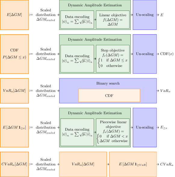
Figure 2: Flowcharts for the calculation of the relevant statistics, from top to bottom: Expectation ($E$), Cumulative Density Function (CDF), Value at Risk ($VaR$), Expectation on a subdomain $\{\Delta GM\geq x\}$ ($E_{\geq x}$), Conditional Value at Risk ($CVaR$). Green boxes represent quantum workloads, while blue boxes are classical workloads. Some metrics are calculated relying upon other ones: specifically, the $VaR$ performs a (classical) binary search over the CDF, which is in turn calculated via a quantum-classical algorithm; similarly, the $CVaR$ is the estimation of the Expected Value on a subdomain determined by the $VaR$, where both the $VaR$ and the Expected Value are determined via quantum-classical algorithms.

4.1 The framework of Quantum Amplitude Estimation for risk analysis

Let us begin with a short introduction of Quantum Amplitude Estimation (QAE), which is the main quantum algorithm we use in this work. Suppose a quantum operator $\mathcal{A}$ acts on an ($n+1$)-qubit state $\ket{0}_{n+1}$ and produces the following state

$$\mathcal{A}\ket{0}_{n+1}=\sqrt{1-a}\ket{\psi_{0}}_{n}\ket{0}+\sqrt{a}\ket{\psi_{1}}_{n}\ket{1}.$$ (2)

Then the QAE [33] approximates the amplitude $a$ in the above equation (2), with an estimate $\tilde{a}$. The error satisfies $\absolutevalue{a-\tilde{a}}=\mathcal{O}(M^{-1})$, where $M$ is the number of applications of $\mathcal{A}$, with probability of at least $8/\pi^{2}$ [4]. The algorithm then extends to any desired confidence level. Therefore a quadratic speed up in the convergence rate is obtained, compared to classical Monte Carlo methods, for which the error is $\mathcal{O}(M^{-1/2})$, where $M$ is the number of Monte Carlo simulations this time.

The idea of QAE and variants, is based on the possibility to construct a Grover operator $\mathcal{Q}$ based on $\mathcal{A}$, whose eigenvectors are related to the desired value $a$ by a trigonometric relationship. Afterwards, the Quantum Phase Estimation is applied to efficiently retrieve the (cosine of) the eigenvectors, and therefore $a$.

Recently, QAE was applied to credit risk analysis and option pricing [2, 4]. The risk analysis with QAE aims at estimating statistics of a random variable $X$, by formulating the problem in such a way that the desired statistics are the amplitudes in Eq. (2).

In order to do so, the first step requires to prepare a quantum state $\ket{\psi}_{n}$ that represents $X$. More explicitey, let $X$ be valued in $\{0,1,...,N-1\}$ with $N=2^{n}$, $n$ being the number of qubits, and let $p_{i}$ be the probability of $X=i$. The encoding operator is $\mathcal{R}$ acting as:

$$\mathcal{R}\ket{0}_{n}=\ket{\psi}_{n}=\sum_{i=0}^{N-1}\sqrt{p_{i}}\ket{i}_{n}$$ (3)

with $i\in\{0,1,...,N-1\}$. Given any relevant quantity in risk analysis, represented by a classical function $f$:

$$f:\{0,1,...,N-1\}\rightarrow[0,1],$$ (4)

suppose we are able to construct a corresponding quantum operator $\mathcal{F}$ such that

$$\mathcal{F}\ket{i}_{n}\ket{0}=\ket{i}_{n}\left[\sqrt{1-f(i)}\ket{0}+\sqrt{f(i)}\ket{1}\right],$$ (5)

for all $i\in\{0,1,...,N-1\}$. Then

$$\begin{split}\mathcal{F}\ket{\psi}_{n}\ket{0}=&\sum_{i=0}^{N-1}\left(\sqrt{1-f(i)}\sqrt{p_{i}}\right)\ket{i}_{n}\ket{0}\\ &+\sum_{i=0}^{N-1}\left(\sqrt{f(i)}\sqrt{p_{i}}\right)\ket{i}_{n}\ket{1}.\end{split}$$ (6)

The probability of measuring $\ket{1}$ in the rightmost qubit is equal to the Expectation of $f$:

$$\sum_{i=0}^{N-1}f(i)\,p_{i}=E\left[f(X)\right].$$ (7)

and the QAE machinery applies to obtain said estimation efficiently. We need to show that our metrics of interest, namely the Expected Value, the Value at Risk, and the Conditional Value at Risk, can be derived from the Expectation of some function $f$.

Let us now move to the Value at Risk. For a confidence level $\alpha\in[0,1]$, $VaR_{\alpha}(X)$ is defined as the smallest value of $X\in\{0,1,...,N-1\}$ such that $\mathbb{P}[X\leq x]\geq(1-\alpha)$, namely

$${VaR}_{\alpha}(X)=\inf\{x\mid\mathbb{P}[X\leq x]\geq 1-\alpha\}.$$ (8)

To find $VaR_{\alpha}(X)$ with QAE, for all $l\in\{0,1,...,N-1\}$, we define a step function

$$f_{l}(i)=\begin{cases}1&\text{if }i\leq l,\\ 0&\text{otherwise.}\end{cases}$$ (9)

Corresponding to $f_{l}$ we further define an operator $\mathcal{F}_{l}$ such that

$$\mathcal{F}_{l}\ket{i}_{n}\ket{0}=\ket{i}_{n}\ket{f_{l}(i)},$$ (10)

so that

$$\mathcal{F}_{l}\ket{\psi}_{n}\ket{0}=\sum_{i=l+1}^{N-1}\sqrt{p_{i}}\ket{i}_{n}\ket{0}+\sum_{i=0}^{l}\sqrt{p_{i}}\ket{i}_{n}\ket{1}.$$ (11)

After implementing QAE, the probability of getting $\ket{1}$ is equal to

$$\sum_{i=0}^{l}p_{i}=\mathbb{P}[X\leq l],$$ (12)

that is the CDF of $X$. Therefore $VaR_{\alpha}(X)$, for a given confidence level $\alpha$, can be retrieved as the smallest $l=l_{\alpha}$ and can be calculated by means of bisection search.

Finally, let us address the conditional Value at Risk $CVaR_{\alpha}(X)$, defined as

$${CVaR}_{\alpha}(X)=E\left[X\mid X\geq VaR_{\alpha}(X)\right].$$ (13)

In words, it is the conditional Expectation of $X$ restricted to $\{0,1,...,l_{\alpha}\}$, where $l_{\alpha}=VaR_{\alpha}(X)$ is defined as before. Then, to estimate $CVaR_{\alpha}(X)$, we define

$$f(i)=\frac{i}{l_{\alpha}}f_{l_{\alpha}}(i)$$ (14)

and the associated operator $\mathcal{F}$ such that

$$\begin{split}&\mathcal{F}\ket{\psi}_{n}\ket{0}=\\ &\left(\sum_{i=l_{\alpha}+1}^{N-1}\sqrt{p_{i}}\ket{i}_{n}+\sum_{i=0}^{l_{\alpha}}\sqrt{1-\frac{i}{l_{\alpha}}}\sqrt{p_{i}}\ket{i}_{n}\right)\ket{0}\\ &\quad\quad+\sum_{i=0}^{l_{\alpha}}\sqrt{\frac{i}{l_{\alpha}}}\sqrt{p_{i}}\ket{i}_{n}\ket{1}.\end{split}$$ (15)

After QAE the probability of getting $\ket{1}$ is equal to $\sum_{i=0}^{l_{\alpha}}\left(\frac{i}{l_{\alpha}}\right)p_{i}$ and $\sum_{i=0}^{l_{\alpha}}p_{i}=P[x\leq l_{\alpha}]$. Therefore we obtain

$$\frac{l_{\alpha}}{\mathbb{P}[X\leq l_{\alpha}]}\sum_{i=0}^{l_{\alpha}}\left(\frac{i}{l_{\alpha}}\right)p_{i}=CVaR_{\alpha}(X)$$ (16)

which also achieves quadratic speedup compared to classical Monte Carlo methods. In our case the random variable $X$ is the delta gross margin $\Delta GM$ defined by (1).

In summary, the three main steps involved in the approach are 1. the distribution loading, 2. the encoding of the objective function, 3. the application of QAE to obtain the relevant statistical quantities. Once we are able to load the data as in Eq. (3), and to encode functions in Eqs. (9) and (14), we can efficiently estimate Expectation, VaR and CVaR. The next subsections are devoted to discussing these requirements.

4.2 Distribution loading

One of the main challenges in quantum computation is how to encode the classical data into a quantum computer efficiently. Our goal is to load a random variable $X$ valued in $\{0,1,...,2^{n}-1\}$ with corresponding probability $p_{i}$ in an $n$-qubit register and form the quantum state

$$\ket{\psi}_{n}=\sum_{i=0}^{2^{n}-1}\sqrt{p_{i}}\ket{i}_{n}.$$ (17)

Let us collect here some of the most prominent approaches in literature. The first one is the qRAM, namely a quantum version of the random access memory (RAM) [34]. From a theoretical perspective, it can be described as a quantum operator allowing efficient (i.e., quantum-parallel) access to classically stored information. Unfortunately though such a device was never built at scale. The second approach is to prepare the desired quantum state directly with controlled rotation gates [35, 36, 37, 38, 39, 40, 41]. The third approach resorts to qGANs for data loading. Out of embeddings, qGAN encoding stands out due to its qubit-efficiency and its capacity to be prepared in a polynomial number of gates using qGANs [42, 43, 44, 45]. This is a popular choice where parametrised quantum circuit with parameter $\theta$ to generate the quantum state

$$\ket{\psi(\theta)}_{n}=\sum_{i=0}^{2^{n}-1}\sqrt{p_{i}(\theta)}\ket{i}_{n}.$$ (18)

In a qGAN the classical generator or discriminator or both is a parametric quantum circuit, thus justifying the term ‘quantum neural network’. Despite of low circuit depth and width of the loading circuits, the training of qGANs is critical both in terms of efficiency and accuracy for an arbitrary and large distribution [46].

As a consequence, we prefer to ground our experiments on controlled rotations.

4.3 Encoding of the objective function

Considering the discussion in Subsec. 4.1, we are interested in piecewise linear functions. Once linear function are available, they can be extended to piecewise linear by resorting to comparators like $F_{l}$ in Eq. (10), that can be easily implemented on quantum computers [47, 5]. As for linear functions, let $f$ be:

$$f(i)=f_{1}i+f_{0}$$ (19)

such that

$$f:\{0,1,...,2^{n}-1\}\rightarrow[0,1].$$ (20)

A quantum operator $\mathcal{F}$ as in Eq. (5) corresponding to the linear function $f$ is in general hard to construct, while it is easy to build $\tilde{\mathcal{F}}$ such that

$$\tilde{\mathcal{F}}\ket{i}_{n}\ket{0}=\ket{i}_{n}\left(\cos[f(i)]\ket{0}+\sin[f(i)]\ket{1}\right).$$ (21)

Therefore it is now a standard [2, 4, 5] to Taylor expand $[\sin f(i)]^{2}$ around a given point, after having introduced a multiplicative constant $C$ in the argument that guarantees the argument is small and therefore the approximation good. Notice that rescaling can be classically accounted as a consequence of the linearity of the involved operations. The approach can also be refined into Fourier expansions of $f$ [48, 49].

5 Circuit optimization and depth reduction techniques

Quantum circuit depth and width minimization as well as gate error mitigation are critical for practical applications of the circuit-based quantum computation. To reduce depth and errors, we follow some hardware optimization techniques, thus getting more accurate result in quantum computers.

5.1 State-of-the-art techniques

After considering all the different sources of error, we selected couple of error mitigation techniques described in the following. Mapomatic addresses the best qubit mapping for a specific device[16]; dynamical decopuling takes care of the qubit decoherence; finally we applied mthree to correct measurement errors; and Pauli Twirling to mitigate gate errors.

Optimal qubit mapping with mapomatic.

To minimize the gate errors in a specific quantum device for a particular quantum circuit, one of the major concerns is to find the best possible mapping between logical qubits and physical qubits in that quantum device. To tackle this issue we use a procedure called mapomatic [16], which is a post-compilation routine that investigates the best low noise sub-graph corresponding to a quantum circuit in the particular target device. The same quantum circuit is transpiled multiple times, to account for the stochastic behavior of the transpiler optimization. The mapomatic ranks the transpiled circuits in terms of the number of the two-qubit gates we target to optimize and finally the best transpiled circuit is picked; for e.g., we choose the circuit with lowest number of swap gates.

Qubit decoherence suppression with dynamical decoupling (DD).

The dynamical decoupling [17] works on physical quantum circuits. It performs a circuit-wide scanning for finding the idle periods of time (those containing delay instructions) and inserts a predefined sequence of gates (for example, a pair of $X$ gates) in those spots. The sequence of gates aggregate to the identity, so that it does not alter the logical action of the circuit, but mitigates the decoherence in those idle periods. For the implementation of DD, one needs the duration of each of the instructions natively supported by the backend and has to choose the sequence of the gates, e.g., a pair of $X$ gates.

Measurement error mitigation with mthree.

Quantum error mitigation techniques are widely used for reducing (mitigating) the errors that occur during quantum executions. For our project we use mthree (M3) [18], a scalable quantum measurement error mitigation technique that does not need the explicit form of the full assignment matrix ($A$-matrix) or its inverse $A^{-1}$. Here, the assignment matrix $A$ is defined as the $2^{N}$ × $2^{N}$ matrix whose element $A_{i,j}$ is the probability of the bit-string $j$ to be converted into the bit-string $i$ as an effect of the measurement error. Instead of characterizing the entire $A$, M3 focuses on the subspace defined by the noisy output bit-strings, thus resorting to a number of calibration matrices that scales at most linearly with the number of qubits.

Gate error mitigation with Pauli Twirling (PT).

In Pauli Twirling (PT), noise channels are approximated as a combination of Pauli gates, so the conjugate of such approximating combination is applied to the circuit to cancel the original noise [19, 50, 51]. PT has become a technique of paramount importance, with implications also in Probabilistic Error Cancellation (PEC) [52] and quantum error correction codes [53]. In this work, we follow the results from Ref. [54], containing an experimental evidence that twirling the circuits between 1 to 8 times aids in error mitigation. For our multi-qubit experimental runs performed in Section 7, we opted to twirl one time and used 5000 shots for each circuit run.

5.2 Approximate Quantum Compiling (AQC)

While computing the relevant statistical quantities using QAE, we encounter quantum circuits with great depth which do not give accurate result on current hardware even after applying the four techniques described above. The general problem of gate compiling is to find an exact representation for a given arbitrary matrix $U\in SU(2^{n})$ using the basis set made of CNOT and single-qubit rotations. It is known that the minimum (sufficient) number of CNOTs needed to compile a general gate is $\lceil\tfrac{1}{4}(4^{n}-3n-1)\rceil$ [55]. An extensive research has been conducted in finding precise decomposition which reach this lower bound [56, 57, 58, 59, 60]. Such lower bound for exact representation is still computationally expensive in terms of circuit depth due to current chip topology and system coherence times.

Alternative approaches to finding circuit simplifications exist. We are interested in the approximate representation, thereby allowing one to move beyond the lower bounds of CNOT cost. Delicate care must be taken not to over-approximate the original circuit. Therefore, we are interested to find an approximate circuit that satisfies a number of hardware constraints (e.g., reduced number of CNOT gates), and is the closest (in some pertinent metric) to the target circuit. Let $U\in SU(2^{n})$ be the unitary matrix induced by the ordered gate sequence of a quantum circuit $\mathcal{S}$ and let $V\in SU(2^{n})$ be another unitary matrix, associated to the approximate circuit. Then the pertinent metric is defined as the distance induced by the Frobenius norm, $||V-U||_{F}$. Ref. [15] provides a method for finding such approximate circuits with a specified number of CNOT gates, called Approximate Quantum Compiling (AQC). The general AQC Problem is defined as:

Definition 1.

Given a target special unitary matrix $U\in SU(2^{n})$ and a set of constraints for example in terms of qubit topology connectivity, find the closest unitary matrix $V\in\mathcal{V}\subseteq SU(2^{n})$, where $\mathcal{V}$ is the set of SU matrices that can be realized by rotations and CNOT gates alone and satisfy those connectivity constraints by solving the following mathematical problem;

$$\mathbf{AQCP:}\quad\min_{V\in\mathcal{V}\subseteq SU(2^{n})}\frac{1}{2}\|V-U\|^{2}_{F}\;.$$ (22)

Given this general problem statement, one can consider so-called "CNOT-units" which are parametrisable 2-qubit circuit blocks consisting of a CNOT gate and pairs of rotations $R_{y}(\theta_{1})$, $R_{z}(\theta_{2})$, $R_{y}(\theta_{3})$, $R_{x}(\theta_{4})$. In this above definition we refer to sets of constraints in terms of qubit topology connectivity. The Qiskit implementation of AQC [61] has several AQC options including the CNOT-tile network geometry: "sequ", "spin", "cart", "cyclic spin", "cyclic line" and inter-qubit connectivity choices of "full", "line", or "star". Details on such configurations can be found in [15] and later in our experimental demonstration we chose the default value of CNOT-tile geometry as "spin" and default qubit topology as "full" (see Figure 3(a)).

One can formulate an alternative form of the AQCP problem as finding the closest unitary matrix $V_{\text{ct}}(\boldsymbol{\theta})$ which results from differing products of CNOT-units as depicted in Figure 3(a), where ct is a parametrized CNOT connectivity structure and $\boldsymbol{\theta}$ is a vector consisting of all parametrized angles $\theta_{i}$ from each of the CNOT-units. The problem can then be reduced to finding

$$\operatorname*{arg\,max}_{\boldsymbol{\theta}}\frac{1}{2^{n}}|\langle V_{\text{ct}}(\boldsymbol{\theta}),U\rangle|\;.$$ (23)

The interesting aspect of this problem is that the unitary matrix $V_{\text{ct}}(\boldsymbol{\theta})$ forms a parametric quantum circuit with a pre-specified CNOT count. This means that we are able to specify a target CNOT count (alternatively called depth), and find the closest matrix $V_{\text{ct}}(\boldsymbol{\theta})$ to our original target unitary matrix $U\in SU(2^{n})$.

This AQC procedure is defined and has been explored for finding approximate quantum circuits close to the target original full quantum circuit. In Section 7 we experimentally demonstrate applying AQC to circuits which use up to 8 qubits for computing the Expected Value using the available code as AQC is implemented in Qiskit as a transpiler plugin [61]. Nonetheless, a natural extension motivated by issues stemming from solving the AQC problem using gradient descent approaches for circuits with a high qubit number, is to segment the target quantum circuit into manageable components and running AQC compilation piecewise before recombining again to obtain the final circuit approximation.

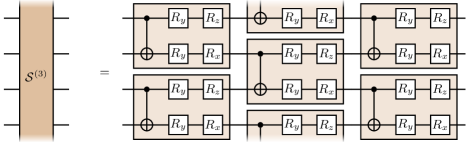
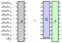
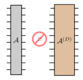
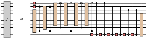
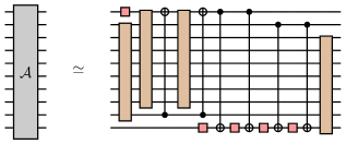
Figure 3: In the above diagrams a schematic description and workflow of pAQC is presented. (a) The standard AQC approximates a gate $\mathcal{S}$ (the brown block in the LHS) with an $\mathcal{S}^{(D)}$ made of $D$ layers ($D=3$ in the picture). Each tile, called a "CNOT-unit", is made of a CNOT gate and four rotations, whose parameters are independent from the other tiles, and determined by the AQC optimization. (b) The operator $\mathcal{A}$, the grey block that we want to approximate with pAQC is $\mathcal{F}\left(\mathcal{R}\otimes I\right)$, are represented with the green and purple blocks respectively. This is the basic building block for the Grover operator. (c) If the number of qubits is high (10 qubits in the picture), the application of AQC is prohibitive due to the lack of convergence of the optimizer. (d) pAQC is then of help. AQC is applied to each brown block, which is identified as to span at most $m=7$ contiguous qubits. The drawing is relative to our specific $\mathcal{A}$. (e) Same decomposition technique as before, except that the parameter $m$ is now $8$.

5.3 Piecewise Approximate Quantum Compiling (pAQC)

Input : Target/original Quantum Circuit $\mathcal{Q}$, maximum subcircuit qubit register span $m$, target individual AQC CNOT depth $D$

Output : Approximated Quantum Circuit $\mathcal{Q}_{\text{approx}}$

STEP 1: Determine subcircuit set $S=\{{\mathcal{Q}_{i}}\}$ via any block identification technique where each $\mathcal{Q}_{i}$ act on quantum register sizes at most $m$ qubits

STEP 2: Compute AQC on each subcircuit

for $Q_{i}$ in S do

       calculate the unitary matrix representation $U_{i}$ of the subcircuit $Q_{i}$,

       compute the AQC approximation $V_{i}:=\text{AQC}(U_{i})$ using target depth $D$,

       convert the unitary approximation $V_{i}$ of each subcircuit $Q_{i}$ back into the AQC CNOT-blocks $\widetilde{Q}_{i}$

STEP 3: Reinsert each newly obtained AQC subcircuit block ${\widetilde{Q}_{i}}$ into the original quantum circuit (replacing $\mathcal{Q}_{i}$) to obtain a new complete quantum circuit $\mathcal{Q}_{\text{approx}}$ which consists of inserted optimized CNOT-blocks via AQC compiling and original circuit components/gates which span qubit sizes on the register greater than $m$ (and hence would affect the convergence of AQC if ran on the full circuit $\mathcal{Q}$

STEP 4: return $\mathcal{Q}_{\text{approx}}$

Algorithm 1 Piecewise Approximate Quantum Compiling (pAQC) of a quantum circuit

It is known that AQC compiling fails to converge for high-dimensional $U\in SU(2^{n})$ matrices due to Barren Plateau phenomena, and as such, other approaches have been proposed to sidestep the issue [62]. In our case, we propose a technique called Piecewise Approximate Quantum Compiling (pAQC) which applies AQC to appropriately identified subcircuits, here called blocks, see Algorithm 1. The central idea of the technique is that instead of approximating the full unitary matrix $U$ representing the quantum algorithm by some ‘close enough’ unitary matrix $V$, we first factor the target matrix into a product of $k$ unitary matrices as $U=U_{1}U_{2}\cdots U_{k}$ such that each unitary matrix $U_{i}$ is a tensor product defined as $U_{i}:=W_{1}\otimes W_{2}\otimes\dots\otimes W_{p}$ where each unitary matrix $W_{j}$ acts on at most $m$ qubits for some suitably chosen size $m$. As we will see, this qubit number $m$ is chosen such that AQC may be applied to each of these subunitary matrices and therefore it cannot be too large e.g. $m\leq 8$. Let $S=\{U_{i}\}^{k}_{i=1}$ denote the set of unitary piecewise partitions/factors of the original target unitary. We wish to apply AQC compiling to elements of $S$ (specifically on unitaries $W_{j}$ which make up each element $U_{i}\in S$) as $V_{i}:=\text{AQC}(U_{i}):=\text{AQC}(W_{1})\otimes\text{AQC}(W_{2})\otimes\dots\otimes\text{AQC}(W_{p})$ and then recombine the individual products to create a new approximate unitary representation of the entire target matrix $V^{\prime}:=V_{1}V_{2}\dots V_{k}$. Note that in general, it is not necessary to apply AQC approximation to every element of the tensor product making up each unitary $U_{i}$ e.g. if $W_{1}=\text{Id}_{2}$. This procedure is described in Algorithm 1.

Since typical AQC compiling of a target unitary matrix has a target CNOT depth $D$ for a single $\text{SU}(2^{n})$ matrix, it is clear that the total circuit depth of a circuit which undergoes $k$-AQC compilations will be greater than or equal to $kD$. Of course, it is also possible to define different strategies where each individual AQC compilation of a circuit slice may have different target depths but for this work we assume they all undergo the same target depth compilation.

Note that the idea of operating on subcircuits has some commonalities with the ‘circuit cutting’ in literature [63, 64]: in that case, though, subcircuits are chosen to have little interactions and are therefore executed independently and then recombined. Compared to such techniques, our objective is simpler and allows for less constrained choices of blocks: we only need to identify subcircuits of $m$ qubits at most, made of adjacent layers in time, on which to apply AQC. Multiple identification methods are possible, including the cutting techniques in literature, which though would result non-optimal in this context. For simplicity, in our proof of principle, we employ the following rule: we consider the blocks of maximal depth made of at most $m$ contiguous qubits. An example for the $9$-qubit quantum circuit for the Expected Value risk measure is depicted in Fig. 7, where we compare the pAQC result when choosing circuit cutting span of $m=7$ in Fig. 7(d) and $m=8$ qubits in Fig. 7(e).

Our experimental demonstration is shown in Section 7, for distributions of 9 and 10 qubits, with qubit register size limit $m=7$. The number $m=7$ is chosen empirically as the AQC problem is known to have limited convergence for higher qubit counts [62]. Additionally, to keep the total gate depth down to an amount which can justifiably run on IBM Quantum hardware, we chose a target CNOT depth of 10 for each partial AQC compilation.

6 Dynamic Amplitude Estimation

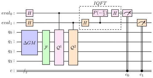
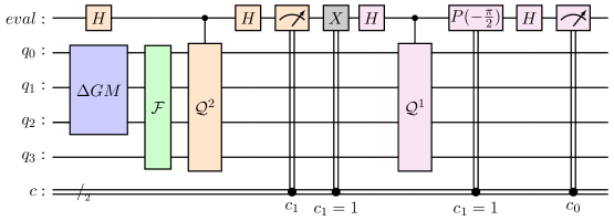
Figure 4: Quantum circuits for computing $E[\Delta GM]$ with two binary digits precision using (a) QAE and (b) DAE respectively. Colours help identify the gates relative to the first power (in pink) and the second power (in yellow). In DAE, the controlled $P$ gate is replaced by a classically conditioned gate through the differed measurement principle. The additional conditioned $X$ gate resets the $eval$ qubit. In QAE two $eval$ qubits used for two binary digit precision (i.e. two iterations), whereas in DAE a single $eval$ qubit is sufficient.

In this section we describe a modified version of QAE using dynamic circuits, a Dynamic Amplitude Estimation (DAE).

In a recent development from IBM Quantum [20], a new quantum hardware feature was introduced, namely Dynamic circuits, which incorporate classical processing within the coherence time of the qubits. Dynamic circuits can assist in overcoming some of the limitations of quantum computer. Many critical applications, such as solving linear systems of equations, make use of auxiliary qubits as working space during a computation and features like mid-circuit measurements, consisting of the ability to perform quantum measurements while the circuit execution is not yet terminated. The technique was used for instance to validate the state of a quantum computer in the presence of noise, allowing for post-selection of the final measurement outcomes based on the success of one or more sanity checks [65, 66, 67]. Related to mid-circuit measurements, also mid-resets were introduced: a qubit, once used, can be returned to the ground state with high-fidelity, so that it is newly available to be used for storage of additional data or for ancillas, thus reducing the total qubit count required in many algorithms [20]. Physically speaking, a qubit reset is a conditional application of the bit-flip gate $X$: more precisely, a projective measurement of the qubit is performed, and if the result is $1$, the state is flipped from $\ket{1}$ to the $\ket{0}$. If the result is a $0$, nothing is done. Note that a qubit mid-reset implies its mid-measurement. The idea of conditioning the application of an $X$ gate to a previous measurement, that is present in the mid-reset, was also extended to any gate or set of gates (sub circuit), giving rise to the so-called conditional operations. Many of IBM Quantum’s hardware backends have been upgraded to support dynamic circuits, released in open-qasm3 [68].

Target	Simulator/	Algorithm	Iterations	Scaled	Unscaled
statistic	Backend			result	result
$E[\Delta GM]$	Exact value	Exact	N/A	8.134	10,913,634
	statevector simulator	IAE	2	7.747	10,883,563
$VaR70[\Delta GM]$	Exact value	Exact	N/A	9.0	10,980,925
	statevector simulator	IAE	2	9.0	10,980,925
$CVaR70[\Delta GM]$	Exact value	Exact	N/A	10.8231	11,122,585
	statevector simulator	IAE	2	18.0663	11,685,403

Table 1: In the above table, the Expectation, $VaR70$, and $CVaR70$ of a 4-qubit $\Delta GM$-distribution are computed exactly and with qasm simulator respectively. By iterations of IAE, we mean the number of quantum-classical interactions. For computing the above statistical quantities with IAE we scale the range of $\Delta GM$-distribution to $[0,15]$. The corresponding original unscaled values are obtained from the scaled results using Eq. (24).

The development of DAE involves two main steps. In the first step we replace the usual Quantum Phase Estimation (QPE) [8] inside QAE with the Iterative Phase Estimation (IPE) [69, 70], thus getting an advantage by reducing the number of qubits, therefore decreasing the costs in terms of noise and hardware requirements. In the second step we further replace the IPE with the Dynamic (Iterative) Phase Estimation (DPE) [20], obtaining an advantage over classical quantum feedback/communication time. IPE substitutes the usual Quantum Fourier Transform present in QPE with phase correction terms, which are implemented iteratively and need only a single auxiliary qubit. The accuracy of the algorithm is restricted by the number of iterations rather than the number of counting qubits. IPE builds the phase from the least to the most significant bit. In the iteration corresponding to the $k$-th binary digit, the phase corrections are applied according to the outcomes of the previous iterations, that have estimated the digits $k+1,...,m$. This way, the circuit for a given iteration is generated after observing the outcome of the previous iterations.

In DPE, each phase correction term is replaced with a sequence of conditional controlled rotation gates using dynamic circuits. The number of significant binary digits provided by DPE equals the number of iterations. In Fig. 4, we present two schematic diagrams comparing canonical QAE and DAE using dynamic circuits for computing the mean of a 3-qubit gross margin distribution ($E[\Delta GM]$). From the quantum circuits we see that the QPE part in QAE is replaced by DPE in DAE, which reduces the number of evaluation qubits.

Let us emphasize here that, despite QPE being present as a subcircuit in the QAE, the proof of the correctness of QAE does not ground straight-forwardly on that of QPE. In fact, QAE does not produce exactly the hypothesis in which the general theory of QPE holds, and more specifically, the operators $\Delta GM$ and $\mathcal{F}$ do not load an eigenvector of the associated Grover oracle $\mathcal{Q}$. On the contrary, they prepare a state which is the weighted sum of two eigenvectors of $\mathcal{Q}$ corresponding to opposite eigenvalues [3]. As a consequence, we cannot directly infer the correctness of DAE from the equivalence between DPE and QPE.

The proof of correctness is anyway very simple, and it grounds on the equivalence between the circuit of QAE and that of DAE. Indeed, referring to Fig. 4(a), the controlled powers of $\mathcal{Q}$ commute, and the blue measurement can be anticipated before the controlled-phase gate transforming into a conditioned gate thanks to the principle of deferred measurement [71, Ch. 4.4], so that it is possible to group all the red gates at the end. The argument easily extends to higher order of powers. From the equivalence of the circuits, it also follows that DAE has the same oracle and query complexity of QAE.

7 Experimental results

In this section, the relevant statistical quantities (mean, VaR, and CVaR) of a $\Delta GM$ distribution are computed, first classically, then implementing QAE, and finally with DAE.

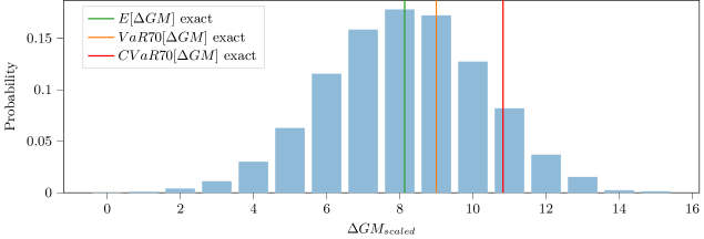
Figure 5: The Expectation, $VaR70$, and $CVaR70$ of a 4-qubit $\Delta GM$ distribution are presented. Note that, in the above plot the range of $\Delta GM$ distribution is scaled to $[0,15]$; therefore the term $\Delta GM_{scaled}$ is used in the X-axis.

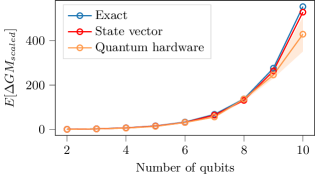
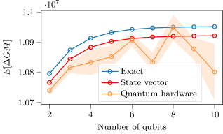
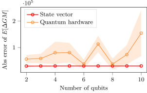
Figure 6: Experimental results for $E[\Delta GM]$ and the corresponding errors, using IAE and without using error mitigation and circuit optimization, are presented in the above plots. Number of qubits in the X-axes of the above plots are the number of qubits used for the distribution loading, which represents the size of the $\Delta GM$-distribution. In Fig.(a), we plot the Expectations of the $\Delta GM_{scaled}$ against the number of qubits. The term $E[\Delta GM_{scaled}]$ means that the $\Delta GM$ is rescaled to $[0,...,2^{n}-1]$. In Fig.(b), the $E[\Delta GM]$ values are plotted in its original scale. Fig.(c) represents the absolute errors of the originally-scaled $E[\Delta GM]$, and in Fig.(d) the relative errors of $E[\Delta GM]$ are plotted as functions of the number of qubits. Relative errors are computed with respect to the exact results. The blue, red and orange curves represent the results obtained from exact computation, state vector simulator and quantum hardware respectively. Each experiment is repeated five times in quantum computer and the shaded regions represent the standard deviations of the quantum computer results around the mean value.

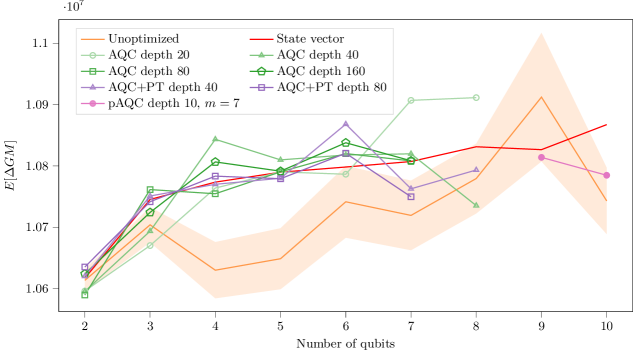
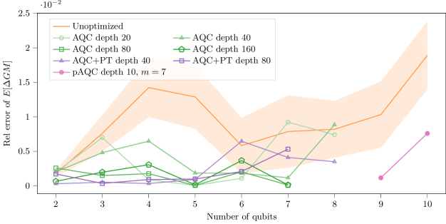
Figure 7: Experimental results for $E[\Delta GM]$ and the corresponding percentage errors with IAE using error mitigation and circuit optimization techniques are presented above. In Fig.(a) the $E[\Delta GM]$ values and in Fig.(b) the relative errors of $E[\Delta GM]$ are plotted as a function of the number of qubits. Relative errors are computed with respect to the statevector results. Note that the number of qubits ($n$) in the X-axes of the above plots are the number of qubits used for the $2^{n}$-dimensional distribution loading; these are not the number of qubits in the quantum circuit after transpilation. The orange and red curves represent the results obtained from the quantum computer and state vector simulator respectively. The other colored lines represent the various types of optimized circuit runs: AQC at target CNOT depth, AQC+PT (Pauli Twiling) represents AQC with additional single PT operation before and after every CNOT gate, and finally, pAQC is used for 9 and 10 qubit data loading where typical AQC-compiling is unstable. Each experiment is repeated 5 times in quantum computer. For easier readability, the shaded regions representing the standard deviations of the quantum computer results are shown only around the unoptimized circuit, whereas all other curves and points are the mean values from the 5 experimental runs.

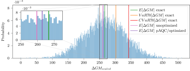
Figure 8: Effect of pAQC/optimized circuit execution on 9-qubit experimental data are shown above. The background distribution represents the complete data set we load into the quantum computer. Coloured vertical lines are the classically computed risk metrics and the calculations of the Expected Value obtained on quantum hardware IBM Mumbai The inset is a zoom of the area around the Expectation, highlighting that the optimization techniques have an improving effect. The detailed hardware results on IBM Mumbai are collected in Figure 7. For the computational purpose we scale the range of $\Delta GM$ to $[0,...,2^{9}-1]$; therefore, the $E[\Delta GM_{scaled}]$ in the X-axis designates the scaled values of original $\Delta GM$.

7.1 Input data and preliminary cases

In this work we consider a simplified weather-related portfolio which depends on gas and temperature. We also consider a one-year time horizon from 1-Jan-2022 to 31-Dec-2022, with daily granularity. The gas prices $[E^{\prime}_{j}]$ and the temperatures $[T^{\prime}_{j}]$ for $j=0,1,...,364$ are are generated by a two-factor Markov model with $2$ normally distributed random variables, which are assumed to be mutually correlated. We consider $R$ Monte Carlo repetitions to generate random samples of temperatures and gas prices. With the temperature and gas price samples we calculate the change of gross margin ($\Delta GM$), defined in Eq.(1). The generation of $\Delta GM$ is described in our previous work [72]. We prepare 10,000 different values of $\Delta GM$ from a Monte Carlo simulation and a probability distribution with $2^{n}$ probability values, where $n$ is the number of qubits available for the data encoding. In this first example, we take $n=4$.

The statistical quantities of $\Delta GM$ are calculated on a noiseless simulator as a preliminary test, using IAE. The 4-qubit probability distribution is loaded in the quantum computer in amplitude encoding, using the procedure described in Ref. [41]. For computational purposes, we need to translate and rescale the range of $\Delta GM$ from $[M_{1},M_{2}]$ to $[0,2^{n}-1]$, with $n$ being the number of qubits to encode the distribution. In our case, $M_{1}=10,281,599$, $M_{2}=11,524,845$ and $n=4$. The result is rescaled back with the following formula:

$$\Delta GM=M_{1}+\left(\frac{M_{2}-M_{1}}{N}\right)\Delta GM_{scaled}.$$ (24)

The results are collected in Table 1 together with the exact results of the discretized distribution.

7.2 Non-optimized runs on quantum hardware

In the previous subsection we have calculated the Expectation, VaR, and CVaR for a random variable with 4-qubit probability distribution using a simulator, with the IAE method. Now we use quantum computer instead, to compute the Expectation. We consider the distribution for $\Delta GM$ containing $10,000$ values defined in Subsec. 7.1, and divide them into $N=2^{n}$ bins, where $n=2,3,...,10$ are the number of desired qubits we want to encode the data into.

In Fig. 6, we present the results for $E[\Delta GM]$ using a quantum computer (IBM Kolkata), without applying the optimization methods in Sec. 5. We used 5000 number of shots for each experiment. For each qubit amount $n=2,3,...,10$, the experiment is repeated five times, and the mean and standard deviation of their results are visualised.

7.3 Effect of circuit optimization and noise mitigation

Target	Simulator/	Algorithm	Iterations	Scaled	Unscaled
statistic	Backend			result	result
$E[\Delta GM]$	Exact value	Exact	N/A	3.8487	10,879,709
	qasm simulator	QAE	2	3.5	10,825,519
	qasm simulator	IAE	2	3.6389	10,847,105
	qasm simulator	DAE	2	3.5	10,825,519
	IBM Mumbai	QAE	2	3.5	10,825,519
	IBM Geneva	IAE	2	3.5034	10,826,048
	IBM Mumbai	DAE	2	3.5	10,825,519
$VaR70[\Delta GM]$	Exact value	Exact	N/A	4	10,903,222
	qasm simulator	QAE	2	3	10,747,816
	qasm simulator	IAE	2	4	10,903,222
	qasm simulator	DAE	2	3	10,747,816
	IBM Geneva	IAE	2	3	10,747,816
	IBM Mumbai	IAE	2	7	11,369,439
	IBM Mumbai	DAE	2	3	10,747,816
$CVaR70[\Delta GM]$	Exact value	Exact	N/A	5.2229	11,093,268
	qasm simulator	QAE	2	5.5327	11,141,412
	qasm simulator	IAE	2	8.3659	11,581,708
	qasm simulator	DAE	2	5.5327	11,141,412
	IBM Geneva	QAE	2	9.4449	11,749,391
	IBM Mumbai	IAE	2	0	10,281,599
	IBM Mumbai	DAE	2	9.4449	11,749,391

Table 2: Result summary for computing $E[\Delta GM]$, $VaR70[\Delta GM]$, and $CVaR70[\Delta GM]$ with QAE, IAE and DAE with qasm simulator and quantum computer for $n=3$ qubits. By iterations of IAE, we mean the number of quantum-classical interactions, while for the other methods we mean the number of oracle powers. For the hardware implementation the circuit depth is reduced using AQC. Given the low number of qubits, there is no need for pAQC. For computing the above statistic with IAE, QAE, and DAE, we scale the range of $\Delta GM$-distribution to $[0,7]$. The corresponding unscaled results are obtained using Eq. (24).

Using the error mitigation and circuit optimization techniques introduced in Section 5, we compute the Expected Value risk measure of the $\Delta GM$ distribution for $n=2$ to $10$ qubits. Fig. 7 summarizes the outcomes of such experiments in quantum computer and gives a comparison against the non-optimized case. Each hardware experiment is performed five times and we use 5000 number of shots for each experiment. We implement mapomatic, DD, mthree error mitigation, and PT for 2 to 10 qubit experiments. For circuit-depth reduction we use AQC for 2 to 8 qubit circuits. For 9 and 10 qubit experiments, we use pAQC because from 9 qubit onward the AQC compilation fails due to Barren plateau phenomena. For AQC we experimented with different target depths, for e.g., 20, 40, 80, and 160, and the experimental results are plotted in different colors in symbols in Fig. 7. For 40 and 80 AQC depth we compared with and without Pauli Twirling one time, and in general, we see that across the multiple qubit and experimental runs up to 7 qubit data loading size, the Pauli-twirled circuit resulted in more accurate estimates (although within each others variance bounds). For pAQC we use 6 blocks of subcircuits with span $m=7$ qubits and in each block we use AQC with target depth of 10. Since AQC and pAQC approximate the circuit, there is always a depth-accuracy trade-off, and the optimal depth can be chosen with extensive empirical trials. For pAQC also there is a trade off between result-accuracy and span $m$ and number of blocks. In Fig. 8, the relevance of pAQC is explained with a 9-qubit distribution. The $E[\Delta GM]$ is computed with and without pAQC and we see that applying pAQC we get a more accurate result.

7.4 Experiments with DAE

We compare the $E[\Delta GM]$, $VaR70[\Delta GM]$, $CVaR70[\Delta GM]$ computed with QAE, IAE and DAE using Qasm simulator and quantum computer. We use AQC to reduce the circuit depth for real-hardware execution. The result summary is presented in Table 2. Note that, given the low number of qubits, we use directly AQC instead of pAQC to reduce the circuit depth. The result from the quantum computer usually fluctuates from the simulator result due the hardware errors. Therefore, for the consistency purpose we repeat the experiment multiple times in a particular quantum hardware and choose the most probable outcome as the final outcome from the multiple runs. For each experiment we use 5000 shots.

8 Discussion

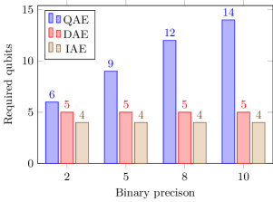
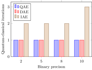
Figure 9: The advantages of DAE over QAE and IAE are represented in the plots above. The binary precision is the number of significant binary digits retrieved for the solution. By increasing the binary precision, on the left we show that DAE uses less qubits than QAE, whereas, on the right the reduction of quantum-classical iterations that DAE brings.

	Queries	QPE	QFT	Aux	Grover	Oracle	Generated
				qubits	oracles	powers	circuits
QAE [33]	$\mathcal{O}(\epsilon^{-1})$	Standard	Yes	$m$	Controlled	$2^{0},...,2^{m-1}$	Single
MLAE EIS [10]	Unknown	Ad hoc	No	$1$	Free	$2^{0},...,2^{m-1}$	MP
QAES [12]	$\mathcal{O}(\epsilon^{-1})$	Ad hoc	No	$0$	Free	Adaptive	MA
IAE [13]	$\tilde{\mathcal{O}}(\epsilon^{-1})$	Ad hoc	No	$0$	Free	Adaptive	MA
FQAE [73]	$\mathcal{O}(\epsilon^{-1})$	Ad hoc	No	$2$	Free	Adaptive	MA
ChebQAE [14]	$\mathcal{O}(\epsilon^{-1})$	Ad hoc	No	$1$	Free	Adaptive	MA
DAE (this work)	$\mathcal{O}(\epsilon^{-1})$	DPE	No	1	Conditioned	$2^{0},...,2^{m-1}$	Single

Table 3: A summary of the prior QAE techniques, in comparison with the newly introduced DAE. ‘Queries’ is a theoretically-proven upper bound on the query complexity to achieve a precision $\epsilon$, if available. All techniques are substantially comparable, except for MLAE for which no theoretical bound is known. The notation $\tilde{\mathcal{O}}$ is used when polylogarithmic factors are discarded. ‘QPE’ is the underlying quantum phase estimation technique: it can be the standard version [8], the dynamic version (DPE) [69], or an ad hoc method. ‘QFT’ indicates whether the Quantum Fourier Transform is applied. ‘Aux qubits’ is the number of qubits required in addition to those needed for the computation of $F$. Here, $m$ is the number of binary digits needed to represent a precision $\epsilon$, namely $2^{-m}=\epsilon$. The original QAE is the only technique whose number of qubits scales with $m$. ‘Grover oracles’ indicates whether the Grover oracles are applied in a quantum-controlled fashion (implying numerous CNOT gates and high associated error), in a classically-conditioned way (implying dynamic circuits and associated circuit delays), or without any control (implying multiple circuits, see last column). ‘Oracle powers’ indicates which oracle powers are evaluated by the algorithm. ‘Generated circuits’ can either be: single (all powers are evaluated through the same circuit), MP (multiple parallelizable, meaning that each oracle power is associated to a different circuit, that can be generated a priori) or MA (multiple adaptive, meaning that each oracle power has an associated circuit, and the power at each iteration is determined after observing the outcome of the previous iteration). In summary, DAE reduces the number of quantum-classical iterations on one side, and of auxiliary qubits on the other.

In this section we discuss the advantages of our newly developed DAE over usual QAE and IAE along with the error mitigation and circuit optimization techniques we have implemented.

In line with our objectives, the proposed DAE has the same theoretical time complexity as the QAE and IAE, providing a quadratic speed up over classical Monte Carlo simulations. The advantages of DAE over QAE and IAE are shown in Fig. 9. Compared to QAE, DAE uses a reduced circuit width: $\mathcal{O}(n)$ qubits for DAE compare to $\mathcal{O}(n+m)$ for QAE, where $n$ is the number of qubits needed for the objective function and $m$ is the number of significant binary digits required in the phase estimation. DAE requires one qubit more than IAE for the evaluation. Since the additional qubit is reset and reused, DAE and IAE have the same order of width. In IAE, each iteration is quantum-classical, and each builds a new quantum circuit, based on the outcome of the previous iteration. The number of quantum-classical iterations in IAE is proportional to the precision digits required for the estimation. On the contrary, in DAE all digits are computed in the same circuit. In Fig. 9, we present a graphical comparison of the above advantages of DAE over QAE and IAE. Table 3 contains a broader comparison of DAE against similar methods. Empirically, DAE has proven to have results in line with QAE on the small problem instances tested in Subsec. 7.4.

For the circuit optimization and error reduction we used multiple methods. The first technique is the optimal qubit mapping for a specific quantum circuit, which is equivalent to find the best low-noise sub-graph. The second one is the ‘dynamical decoupling’, which inserts identity-summing operations on idle qubits, for mitigating the decoherence. Next two applications are called the Pauli Twirling and ‘mthree error mitigation’ which is used for the measurement error mitigation. The fifth one is the approximate quantum compiler (AQC). AQC reduces the CNOT depth of the quantum circuit to a specific target CNOT depth by constructing an approximate version of the original circuit. For instance, in our particular three-qubit $\Delta GM$-distribution case the circuit depths for computing $E[\Delta GM]$ with QAE without using AQC is $4130$ (CNOT count: $1464$) whereas with AQC it is $487$ (CNOT count: $154$) respectively. Finally, to overcome the limitations of AQC for higher circuit width, we implement Piecewise Approximate Quantum Compiling (pAQC) in Sec. 5.3 which applies AQC to appropriate subcircuits. Here we show initial experimental verification that pAQC can be used for 9 and 10 qubit circuits (post transpilation up to 13 physical qubits). However, a deeper experimental analysis concerning the trade-offs between subcircuit indentification rules, individual piecewise AQC depths, and qubit scaling will be part of a follow up work. The joint effect of these techniques, discussed in Subsec. 7.3 and Fig. 7, is to roughly halve the percentage of error. Additionally, pAQC can provide results in line with AQC in terms of error reduction, while being applicable to much wider circuits.

9 Conclusion

In this work, a practical implementation of amplitude estimation methods was demonstrated in the field of energy economics. To do so, we first discussed state-of-the-art methods for error mitigation and circuit optimization, designed to reduce the circuit depth and increase the accuracy of the outcomes: specifically, we considered mapomatic for optimal qubit assignment, dynamical decoupling for qubit decoherence suppression, mthree for measurement error mitigation, Pauli Twirling for coherent gate error mitigation, and AQC for depth reduction via circuit approximation. We contributed with pAQC, an improved version of AQC, suited for wide circuits. Thanks to said techniques, we were able to demonstrate an accurate estimation of the Expectation of the delta gross margin of a portfolio, with an input distribution up to 10 qubits. Finally, we developed DAE, a novel amplitude estimation technique, having an lower width than QAE, and reduced quantum-classical communication overhead than iterative methods such as IAE. The new method is also applied to the calculation of $VaR70$, $CVaR70$ of $\Delta GM$.

We believe this work serves as an important stepping stone in applying quantum risk analysis to real-life data and scenarios on current quantum hardware. The error mitigation techniques used and variants of resource efficient algorithms/compiling demonstrate that by carefully using resources even on today’s noisy quantum devices, we are able to run amplitude estimation algorithms with double-digit qubit number on industry relevant use-cases.

Appendix A Hardware specifications of the IBM devices used for our experiments

In this Appendix we present some of the hardware specifications and calibration details of the IBM devices that were used in this work. We used three quantum devices: IBM Kolkata, IBM Mumbai, IBM Geneva. IBM Geneva has been retired recently, but its specifications can be found in the Appendix G of Ref. [74].

A topology graph of IBM Mumbai is provided in Fig. 10, while Table 4 contains some of its specifications. Similarly, Fig. 11 show the topology graph of IBM Kolkata, and Table 5 presents its specifications.

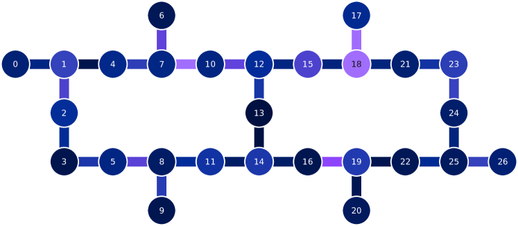
Figure 10: The qubit topology graph of IBM Mumbai, which is 27-qubit quantum device.

Qubit	T1 (us)	T2 (us)	Frequency (GHz)	Anharmonicity (GHz)	Readout assignment error
0	121.893	74.716	5.204	-0.342	0.009
1	184.820	193.854	4.991	-0.345	0.011
2	1.090	44.904	5.113	-0.343	0.015
3	122.597	91.154	4.866	-0.346	0.008
4	137.168	97.225	5.225	-0.341	0.020
5	117.449	28.713	5.113	-0.342	0.033
6	135.955	98.217	5.203	-0.340	0.019
7	117.815	46.209	5.031	-0.346	0.024
8	105.400	59.126	4.928	-0.345	0.036
9	141.072	137.121	5.054	-0.344	0.019
10	101.163	41.160	5.178	-0.342	0.007
11	167.565	34.630	4.868	-0.373	0.137
12	88.162	111.563	4.961	-0.347	0.006
13	141.847	289.065	5.018	-0.346	0.010
14	161.545	239.810	5.118	-0.343	0.064
15	160.563	188.404	5.041	-0.344	0.008
16	72.080	67.929	5.222	-0.340	0.016
17	152.147	40.861	5.236	-0.340	0.004
18	126.501	89.403	5.097	-0.344	0.009
19	116.195	28.216	5.002	-0.345	0.042
20	119.181	17.413	5.187	-0.341	0.017
21	135.261	26.209	5.274	-0.341	0.007
22	136.999	40.839	5.127	-0.343	0.039
23	121.708	56.139	5.138	-0.343	0.005
24	143.578	92.588	5.005	-0.346	0.020
25	231.713	119.274	4.921	-0.347	0.006
26	142.938	155.379	5.120	-0.342	0.043

Table 4: Some of the hardware specifications and calibration details of the IBM Mumbai device are collected in the above table. Using this device we produce the experimental results for $E[\Delta GM]$ and the corresponding errors described in Fig. 6.

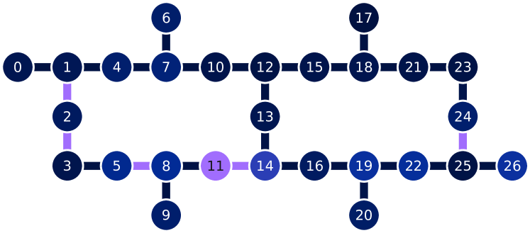
Figure 11: The qubit topology graph of IBM Kolkata, which is a 27-qubit quantum device.

Qubit	T1 (us)	T2 (us)	Frequency (GHz)	Anharmonicity (GHz)	Readout assignment error
0	87.465	260.251	5.071	-0.328	0.019
1	154.965	253.803	4.930	-0.331	0.043
2	123.854	128.832	4.670	-0.337	0.027
3	141.994	102.277	4.889	-0.331	0.011
4	138.323	59.249	5.021	-0.330	0.023
5	112.715	155.115	4.969	-0.330	0.022
6	108.421	77.457	4.966	-0.329	0.013
7	230.526	45.334	4.894	-0.331	0.022
8	174.829	224.879	4.792	-0.333	0.016
9	90.581	151.520	4.955	-0.331	0.012
10	83.077	116.724	4.959	-0.331	0.021
11	167.969	258.766	4.666	-0.333	0.031
12	177.792	313.115	4.743	-0.333	0.026
13	171.273	255.389	4.889	-0.328	0.009
14	86.130	195.007	4.780	-0.333	0.035
15	144.229	37.756	4.858	-0.333	0.048
16	88.207	181.479	4.980	-0.330	0.012
17	78.171	110.120	5.003	-0.330	0.024
18	86.443	195.045	4.781	-0.333	0.079
19	249.517	298.643	4.810	-0.332	0.037
20	128.772	220.638	5.048	-0.328	0.014
21	111.219	220.139	4.943	-0.331	0.018
22	163.283	224.330	4.911	-0.332	0.013
23	136.101	265.180	4.893	-0.332	0.040
24	144.812	49.376	4.671	-0.336	0.017
25	190.122	144.656	4.759	-0.334	0.015
26	44.097	291.006	4.954	-0.330	0.019

Table 5: Some of the hardware specifications and calibration details of the IBM Kolkata device are collected in the above table. Using this device we produce the experimental results for $E[\Delta GM]$ and the corresponding errors described using the circuit optimization and error mitigation techniques in Fig. 7. This device is also used to produce the results for $E[\Delta GM]$, $VaR70[\Delta GM]$, and $CVaR70[\Delta GM]$ with QAE, IAE and DAE described in Table 2.

References

- [1] “Quantum circuits get a dynamic upgrade with the help of concurrent classical computation”. url: https://www.ibm.com/blogs/research/2021/02/quantum-phase-estimation/ (2021).
- [2] Nikitas Stamatopoulos, Daniel J Egger, Yue Sun, Christa Zoufal, Raban Iten, Ning Shen, and Stefan Woerner. “Option pricing using quantum computers”. Quantum 4, 291 (2020).
- [3] Patrick Rebentrost, Brajesh Gupt, and Thomas R. Bromley. “Quantum computational finance: Monte carlo pricing of financial derivatives”. Physical Review A 98, 022321 (2018).
- [4] Stefan Woerner and Daniel J Egger. “Quantum risk analysis”. npj Quantum Information 5, 1–8 (2019).
- [5] Daniel J. Egger, Ricardo Garcia Gutierrez, Jordi Cahue Mestre, and Stefan Woerner. “Credit risk analysis using quantum computers”. IEEE Transactions on Computers 70, 2136–2145 (2021).
- [6] Christian Laudagé and Ivica Turkalj. “Calculating expectiles and range value-at-risk using quantum computers” (2022) arXiv:2211.04456 [quant-ph].
- [7] Emanuele Dri, Antonello Aita, Edoardo Giusto, Davide Ricossa, Davide Corbelletto, Bartolomeo Montrucchio, and Roberto Ugoccioni. “A more general quantum credit risk analysis framework”. Entropy 25, 593 (2023).
- [8] A. Yu. Kitaev. “Quantum measurements and the abelian stabilizer problem” (1995).
- [9] L. K. Grover. “Quantum mechanics helps in searching for a needle in a haystack”. Phys. Rev. Lett. 79, 325 (1997).
- [10] Yohichi Suzuki, Shumpei Uno, Rudy Raymond, Tomoki Tanaka, Tamiya Onodera, and Naoki Yamamoto. “Amplitude estimation without phase estimation”. Quantum Information Processing 19, 75 (2020).
- [11] Chu-Ryang Wie. “Simpler quantum counting”. Quantum Information and Computation 19, 967–983 (2019).
- [12] Scott Aaronson and Patrick Rall. “Quantum Approximate Counting, Simplified”. In Symposium on Simplicity in Algorithms (SOSA). Pages 24–32. Proceedings. Society for Industrial and Applied Mathematics (2019).
- [13] Dmitry Grinko, Christa Zoufal, Julien Gacon, and Stefan Woerner. “Iterative quantum amplitude estimation”. npj Quantum Information 7, 1–9 (2021).
- [14] Patrick Rall and Bryce Fuller. “Amplitude Estimation from Quantum Signal Processing” (2022). arXiv:2207.08628 [quant-ph].
- [15] Liam Madden and Andrea Simonetto. “Best approximate quantum compiling problems”. ACM Transactions on Quantum Computing 3, 1–29 (2022).
- [16] Matthew Treinish et al. “mapomatic: Automatic mapping of compiled circuits to low-noise sub-graphs”. url: https://github.com/Qiskit-Partners/mapomatic (2022).
- [17] Qiskit software developers. “Dynamical decoupling insertion pass”. url: https://qiskit.org/documentation/stubs/qiskit.transpiler.passes.DynamicalDecoupling.html (2022).
- [18] Paul D. Nation, Hwajung Kang, Neereja Sundaresan, and Jay M. Gambetta. “Scalable mitigation of measurement errors on quantum computers”. PRX Quantum 2, 040326 (2021).
- [19] Michael R. Geller and Zhongyuan Zhou. “Efficient error models for fault-tolerant architectures and the pauli twirling approximation”. Phys. Rev. A 88, 012314 (2013).
- [20] A. D. Córcoles, Maika Takita, Ken Inoue, Scott Lekuch, Zlatko K. Minev, Jerry M. Chow, and Jay M. Gambetta. “Exploiting dynamic quantum circuits in a quantum algorithm with superconducting qubits”. Phys. Rev. Lett. 127, 100501 (2021).
- [21] C J O’Loan. “Iterative phase estimation”. Journal of Physics A: Mathematical and Theoretical 43, 015301 (2010).
- [22] Ashley Montanaro. “Quantum speedup of monte carlo methods”. Proceedings of the Royal Society A: Mathematical, Physical and Engineering Sciences 471, 20150301 (2015).
- [23] Emanuel Knill, Gerardo Ortiz, and Rolando D. Somma. “Optimal quantum measurements of expectation values of observables”. Physical Review A 75, 012328 (2007).
- [24] Gabriele Agliardi, Michele Grossi, Mathieu Pellen, and Enrico Prati. “Quantum integration of elementary particle processes”. Physics Letters B 832, 137228 (2022).
- [25] Kazuya Kaneko, Koichi Miyamoto, Naoyuki Takeda, and Kazuyoshi Yoshino. “Linear regression by quantum amplitude estimation and its extension to convex optimization”. Physical Review A 104, 022430 (2021).
- [26] Nathan Wiebe, Ashish Kapoor, and Krysta M Svore. “Quantum perceptron models”. In Proceedings of the 30th International Conference on Neural Information Processing Systems. Pages 4006–4014. NIPS’16. Curran Associates Inc. (2016).
- [27] Iordanis Kerenidis, Jonas Landman, Alessandro Luongo, and Anupam Prakash. “q-means: A quantum algorithm for unsupervised machine learning” (2018) arXiv:1812.03584 [quant-ph].
- [28] P. Glasserman. “Monte Carlo methods in financial engineering”. Springer-Verlag New York. (2004).
- [29] F.E. Benth and J. Saltyte-Benth. “Stochastic modelling of temperature variations with a view towards weather derivatives”. Applied Mathematical Finance 12, 53–85 (2005).
- [30] F.E. Benth and J. Saltyte-Benth. “The volatility of temperature and pricing of weather derivatives”. Quantitative Finance 7, 553–561 (2007).
- [31] L. Cucu, R. Döttling, P. Heider, and S. Maina. “Managing temperature-driven volume risks”. Journal of energy markets 9, 95–110 (2016).
- [32] P. Sabino and N. Cufaro Petroni. “Fast Pricing of Energy Derivatives with Mean-Reverting Jump-diffusion Processes”. Applied Mathematical Finance 0, 1–22 (2021).
- [33] Gilles Brassard, Peter Hoyer, Michele Mosca, and Alain Tapp. “Quantum amplitude amplification and estimation”. Contemporary Mathematics 305, 53–74 (2002).
- [34] V. Giovannetti, S. Lloyd, and L. Maccone. “Quantum random access memory”. Phys. Rev. Lett. 100, 160501 (2008).
- [35] A. Barenco and Bennett et al. “Elementary gates for quantum computation”. Phys. Rev. A 52, 3457 (1995).
- [36] P. Kumar. “Direct implementation of an n-qubit controlled-unitary gate in a single step”. Quantum information processing 12, 1201–1223 (2013).
- [37] J. A. Cortese and T. M. Braje. “Loading classical data into a quantum computer” (2018). url: arxiv.org/abs/1803.01958.
- [38] M. Plesch and Časlav Brukner. “Quantum-state preparation with universal gate decompositions”. Phys. Rev. A 83, 032302 (2011).
- [39] Dan Ventura and Tony Martinez. “Initializing the amplitude distribution of a quantum state”. Foundations of Physics Letters 12, 547–559 (1999).
- [40] Israel F Araujo, Daniel K Park, Francesco Petruccione, and Adenilton J da Silva. “A divide-and-conquer algorithm for quantum state preparation”. Scientific Reports 11, 1–12 (2021).
- [41] Israel F. Araujo, Daniel K. Park, Teresa B. Ludermir, Wilson R. Oliveira, Francesco Petruccione, and Adenilton J. da Silva. “Configurable sublinear circuits for quantum state preparation”. arXiv:2108.10182 [quant-ph] (2022). arXiv:2108.10182.
- [42] Christa Zoufal, Aurélien Lucchi, and Stefan Woerner. “Quantum generative adversarial networks for learning and loading random distributions”. npj Quantum Information 5, 1–9 (2019).
- [43] Daniel Herr, Benjamin Obert, and Matthias Rosenkranz. “Anomaly detection with variational quantum generative adversarial networks”. Quantum Science and Technology 6, 045004 (2021).
- [44] Shouvanik Chakrabarti, Huang Yiming, Tongyang Li, Soheil Feizi, and Xiaodi Wu. “Quantum wasserstein generative adversarial networks”. Advances in Neural Information Processing Systems32 (2019).
- [45] Raúl Berganza Gómez, Corey O’Meara, Giorgio Cortiana, Christian B Mendl, and Juan Bernabé-Moreno. “Towards autoqml: A cloud-based automated circuit architecture search framework” (2022).
- [46] Gabriele Agliardi and Enrico Prati. “Optimal Tuning of Quantum Generative Adversarial Networks for Multivariate Distribution Loading”. Quantum Reports 4, 75–105 (2022).
- [47] Thomas G Draper, Samuel A Kutin, Eric M Rains, and Krysta M Svore. “A logarithmic-depth quantum carry-lookahead adder”. Quantum Information & Computation 6, 351–369 (2006). url: dl.acm.org/doi/abs/10.5555/2012086.2012090.
- [48] Steven Herbert. “Quantum monte carlo integration: The full advantage in minimal circuit depth”. Quantum 6, 823 (2022).
- [49] Jorge J. Martínez de Lejarza, Michele Grossi, Leandro Cieri, and Germán Rodrigo. “Quantum fourier iterative amplitude estimation” (2023) arXiv:2305.01686 [hep-ph, physics:quant-ph].
- [50] Abhinav Kandala, Kristan Temme, Antonio D Corcoles, Antonio Mezzacapo, Jerry M Chow, and Jay M Gambetta. “Extending the computational reach of a noisy superconducting quantum processor”. Nature 567, 491–495 (2019).
- [51] Zhenyu Cai and Simon C Benjamin. “Constructing smaller pauli twirling sets for arbitrary error channels”. Scientific reports 9, 11281 (2019).
- [52] Ewout van den Berg, Zlatko K Minev, Abhinav Kandala, and Kristan Temme. “Probabilistic error cancellation with sparse pauli-lindblad models on noisy quantum processors” (2022).
- [53] Amara Katabarwa and Michael R Geller. “Logical error rate in the pauli twirling approximation”. Scientific reports 5, 1–6 (2015).
- [54] Youngseok Kim, Christopher J Wood, Theodore J Yoder, Seth T Merkel, Jay M Gambetta, Kristan Temme, and Abhinav Kandala. “Scalable error mitigation for noisy quantum circuits produces competitive expectation values”. Nature Physics (2023).
- [55] Vivek V Shende, Igor L Markov, and Stephen S Bullock. “Minimal universal two-qubit controlled-not-based circuits”. Physical Review A 69, 062321 (2004).
- [56] Sumeet Khatri, Ryan LaRose, Alexander Poremba, Lukasz Cincio, Andrew T Sornborger, and Patrick J Coles. “Quantum-assisted quantum compiling”. Quantum 3, 140 (2019).
- [57] Lukasz Cincio, Yiğit Subaşı, Andrew T Sornborger, and Patrick J Coles. “Learning the quantum algorithm for state overlap”. New Journal of Physics 20, 113022 (2018).
- [58] Péter Rakyta and Zoltán Zimborás. “Efficient quantum gate decomposition via adaptive circuit compression” (2022).
- [59] Péter Rakyta and Zoltán Zimborás. “Approaching the theoretical limit in quantum gate decomposition”. Quantum 6, 710 (2022).
- [60] Peter Rakyta, Gregory Morse, Jakab Nádori, Zita Majnay-Takács, Oskar Mencer, and Zoltán Zimborás. “Highly optimized quantum circuits synthesized via data-flow engines” (2022).
- [61] “Approximate Quantum Compiler - Qiskit”. https://qiskit.org/documentation/apidoc/synthesis_aqc.html. Accessed: 2023-04-01.
- [62] Liam Madden, Albert Akhriev, and Andrea Simonetto. “Sketching the best approximate quantum compiling problem”. In 2022 IEEE International Conference on Quantum Computing and Engineering (QCE). Pages 492–502. IEEE (2022).
- [63] Tianyi Peng, Aram W Harrow, Maris Ozols, and Xiaodi Wu. “Simulating large quantum circuits on a small quantum computer”. Physical review letters 125, 150504 (2020).
- [64] Wei Tang, Teague Tomesh, Martin Suchara, Jeffrey Larson, and Margaret Martonosi. “CutQC: using small quantum computers for large quantum circuit evaluations”. In Proceedings of the 26th ACM International Conference on Architectural Support for Programming Languages and Operating Systems. Pages 473–486. ASPLOS ’21. Association for Computing Machinery (2021).
- [65] Sam McArdle, Xiao Yuan, and Simon Benjamin. “Error-mitigated digital quantum simulation”. Physical Review Letters 122, 180501 (2019).
- [66] Ruslan Shaydulin and Alexey Galda. “Error mitigation for deep quantum optimization circuits by leveraging problem symmetries”. In 2021 IEEE International Conference on Quantum Computing and Engineering (QCE). Pages 291–300. IEEE (2021).
- [67] Ludmila Botelho, Adam Glos, Akash Kundu, Jarosław Adam Miszczak, Özlem Salehi, and Zoltán Zimborás. “Error mitigation for variational quantum algorithms through mid-circuit measurements”. Physical Review A 105, 022441 (2022).
- [68] Andrew Cross, Ali Javadi-Abhari, Thomas Alexander, Niel De Beaudrap, Lev S. Bishop, Steven Heidel, Colm A. Ryan, Prasahnt Sivarajah, John Smolin, Jay M. Gambetta, and Blake R. Johnson. “Openqasm 3: A broader and deeper quantum assembly language”. ACM Transactions on Quantum Computing3 (2022).
- [69] Miroslav Dobšíček, Göran Johansson, Vitaly Shumeiko, and Göran Wendin. “Arbitrary accuracy iterative quantum phase estimation algorithm using a single ancillary qubit: A two-qubit benchmark”. Phys. Rev. A 76, 030306 (2007).
- [70] Joseph G. Smith, Crispin H. W. Barnes, and David R. M. Arvidsson-Shukur. “An iterative quantum-phase-estimation protocol for near-term quantum hardware” (2022).
- [71] M. A. Nielsen and I. L. Chuang. “Quantum computation and quantum information”. Cambridge University Press. Cambridge (2001).
- [72] Gabriele Agliardi, Corey O’Meara, Kavitha Yogaraj, Kumar Ghosh, Piergiacomo Sabino, Marina Fernández-Campoamor, Giorgio Cortiana, Juan Bernabé-Moreno, Francesco Tacchino, Antonio Mezzacapo, and Omar Shehab. “Quadratic quantum speedup in evaluating bilinear risk functions” (2023) arXiv:2304.10385.
- [73] Kouhei Nakaji. “Faster amplitude estimation”. Quantum Information and Computation 20, 1109–1123 (2020). arXiv:2003.02417 [quant-ph].
- [74] Norhan M Eassa, Joe Gibbs, Zoe Holmes, Andrew Sornborger, Lukasz Cincio, Gavin Hester, Paul Kairys, Mario Motta, Jeffrey Cohn, and Arnab Banerjee. “High-fidelity dimer excitations using quantum hardware” (2023).