Contrastive Label Enhancement

Abstract

Label distribution learning (LDL) is a new machine learning paradigm for solving label ambiguity. Since it is difficult to directly obtain label distributions, many studies are focusing on how to recover label distributions from logical labels, dubbed label enhancement (LE). Existing LE methods estimate label distributions by simply building a mapping relationship between features and label distributions under the supervision of logical labels. They typically overlook the fact that both features and logical labels are descriptions of the instance from different views. Therefore, we propose a novel method called Contrastive Label Enhancement (ConLE) which integrates features and logical labels into the unified projection space to generate high-level features by contrastive learning strategy. In this approach, features and logical labels belonging to the same sample are pulled closer, while those of different samples are projected farther away from each other in the projection space. Subsequently, we leverage the obtained high-level features to gain label distributions through a well-designed training strategy that considers the consistency of label attributes. Extensive experiments on LDL benchmark datasets demonstrate the effectiveness and superiority of our method.

1 Introduction

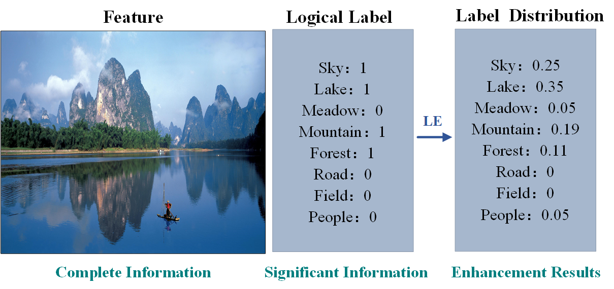
Figure 1: An example of label enhancement. Features contain the full information of samples with many redundancies, while logical labels possess significant information but are not comprehensive. The generation of label distributions makes full use of the important knowledge in logical labels and supplements the sample details according to the features.

In recent years, Label Distribution Learning (LDL) Geng (2016) has drawn much attention in machine learning, with its effectiveness demonstrated in various applications Geng et al. (2013); Zhang et al. (2015); Qi et al. (2022). Unlike single-label learning (SLL) and multi-label learning (MLL) Gibaja and Ventura (2014); Moyano et al. (2019); Zhao et al. (2022), LDL can provide information on how much each label describes a sample, which helps to deal with the problem of label ambiguity Geng (2016). However, Obtaining label distributions is more challenging than logical labels, as it requires many annotators to manually indicate the degree to which each label describes an instance and accurately quantifying this degree remains difficult. Thus, Xu et al. (2019) proposed Label Enhancement (LE), leveraging the topological information in the feature space and the correlation among the labels to recover label distributions from logical labels.

More specifically, LE can be seen as a preprocessing of LDL Zheng et al. (2021), which takes the logically labeled datasets as inputs and outputs label distributions. As shown in Figure 1, this image reflects the complete information of the sample including some details. Meanwhile, its corresponding logical labels only highlight the most salient features, such as the sky, lake, mountain, and forest. Features contain comprehensive information about samples with many redundancies, while logical labels hold arresting information but are not all-sided. Therefore, it is reasonable to assume that features and logical labels can be regarded as two descriptions of instances from different views, possessing complete and salient information of samples. The purpose of LE tasks can be simplified as enhancing the significant knowledge in logical labels by utilizing detailed features. Subsequently, each label is allocated a descriptive degree according to its importance.

Most existing LE methods concentrate on establishing the mapping relationship between features and label distributions under the guidance of logical labels. Although these previous works have achieved good performance for LE problem, they neglect that features and labels are descriptions of two different dimensions related to the same samples. Furthermore, logical labels can only indicate the conspicuous information of each sample without obtaining the label description ranking. The label distributions may appear to be quite different even if the logical labels present the same results.

To address these issues, we propose the ConLE method which fuses features and logic labels to generate the high-level features of samples by contrastive learning strategy. More specifically, we elaborately train a representation learning model, which forces the features and logical labels of the same instance to be close in projection space, while those of different instances are farther away. By concatenating the representations of features and logical labels in projection space, we get high-level features including knowledge of logic labels and features. Accordingly, label distributions can be recovered from high-level features by the feature mapping network. Since it is expected that the properties of labels in the recovered label distributions should be consistent with those in the logical labels, we design a training strategy with label-level consistency to guide the learning of the feature mapping network.

Our contributions can be delivered as follows:

• Based on our analysis of label enhancement, we recognize that features and logical labels offer distinct perspectives on instances, with features providing comprehensive information and logical labels highlighting salient information. In order to leverage the intrinsic relevance between these two views, we propose the Contrastive Label Enhancement (ConLE) method, which unifies features and logical labels in a projection space to generate high-level features for label enhancement.

• Since all possible labels should have similar properties in logical labels and label distributions, we design a training strategy to keep the consistency of label properties for the generation of label distributions. This strategy not only maintains the attributes of relevant and irrelevant labels but also minimizes the distance between logical labels and label distributions.

• Extensive experiments are conducted on 13 benchmark datasets, experimental results validate the effectiveness and superiority of our ConLE compared with several state-of-the-art LE methods.

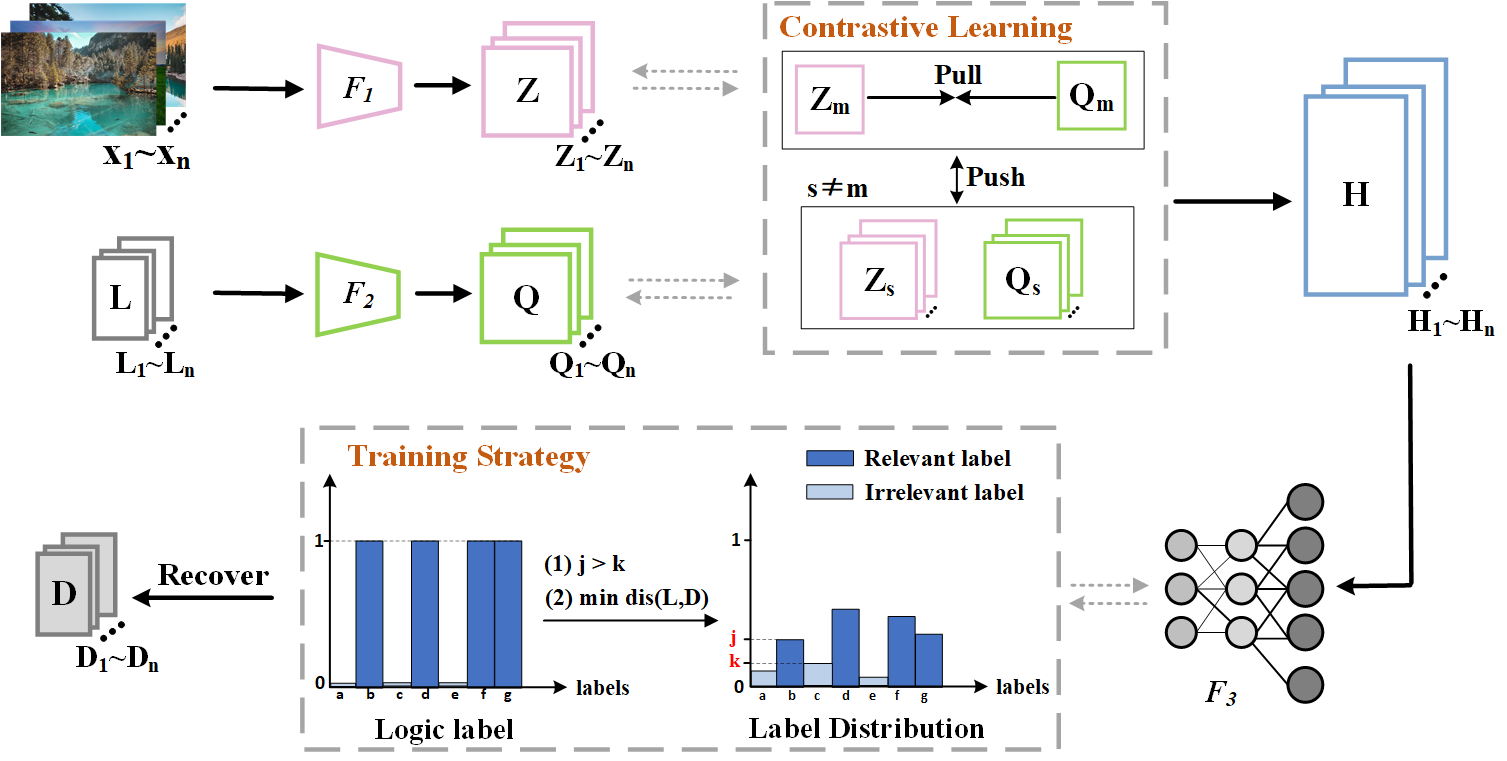
Figure 2: Framework of the proposed ConLE. ConLE approaches the LE problem by regarding features ($X$) and logical labels ($L$) as sample descriptions from two views. It uses two mapping networks ($F_{1}$ and $F_{2}$) to project $X$ and $L$ into a unified projection space, which results in two representations $Z$ and $Q$. These representations are then concatenated into high-level features ($H$). To obtain good high-level features, ConLE utilizes a contrastive learning strategy that brings two representations of the same sample closer together while pushing representations of different samples farther apart from each other. Additionally, ConLE employs a reliable training strategy to generate label distributions $D$ from high-level features $H$ by the feature mapping network $F_{3}$. This strategy minimizes the distance between logical labels and label distributions, ensuring that the restored label distributions are close to the existing logical labels. Meanwhile, it also demands the description degree of relevant labels marked as 1 in the logical labels is larger than that of the irrelevant labels marked as 0. In this way, ConLE can guarantee the consistency of label attributes in logical labels and label distributions.

2 Related Work

In this section, we mainly introduce the related work of this paper from two research directions: label enhancement and contrastive learning.

Label Enhancement.

Label enhancement is proposed to recover label distributions from logical labels and provide data preparation for LDL. For example, the Graph Laplacian LE (GLLE) method proposed by Xu et al. (2021) makes the learned label distributions close to logical labels while accounting for learning label correlations, making similar samples have similar label distributions. The method LESC proposed by Tang et al. (2020) uses low-rank representations to excavate the underlying information contained in the feature space. Xu et al. (2022) proposed LEVI to infer label distributions from logical labels via variational inference. The method RLLE formulates label enhancement as a dynamic decision process and uses prior knowledge to define the target for LE Gao et al. (2021). The kernel-based label enhancement (KM) algorithm maps each instance to a high-dimensional space and uses a kernel function to calculate the distance between samples and the center of the group, in order to obtain the label description. Jiang et al. (2006). The LE algorithm based on label propagation (LP) recovers label distributions from logical labels by using the iterative label propagation technique Li et al. (2015). Sequential label enhancement (Seq_LE) formulates the LE task as a sequential decision procedure, which is more consistent with the process of annotating the label distributions in human brains Gao et al. (2022). However, these works neglect the essential connection between features and logical labels. In this paper, we regard features and logical labels as sample descriptions from different views, where we can create faithful high-level features for label enhancement by integrating them into the unified projection space.

Contrastive Learning.

The basic idea of contrastive learning, an excellent representation learning method, is to map the original data to a feature space. Within this space, the objective is to maximize the similarities among positive pairs while minimizing those among negative pairs. Grill et al. (2020); Li et al. (2020). Currently, contrastive learning has achieved good results in many machine learning domains Li et al. (2021); Dai and Lin (2017). Here we primarily introduce several contrastive learning methods applied to multi-label learning. Wang et al. (2022) designed a multi-label contrastive learning objective in the multi-label text classification task, which improves the retrieval process of their KNN-based method. Zhang et al. (2022) present a hierarchical multi-label representation learning framework that can leverage all available labels and preserve the hierarchical relationship between classes. Qian et al. (2022) propose two novel models to learn discriminative and modality-invariant representations for cross-modal retrieval. Bai et al. (2022) propose a novel contrastive learning boosted multi-label prediction model based on a Gaussian mixture variational autoencoder (C-GMVAE), which learns a multimodal prior space and employs a contrastive loss. For ConLE, the descriptions of one identical sample are regarded as positive pairs and those of different samples are negative pairs. We pull positive pairs close and negative pairs farther away in projection space by contrastive learning to obtain good highlevel features, which is really beneficial for the LE process.

3 The ConLE Approach

In this paper, we use the following notations. The set of instances is denoted by $X=\{x_{1},x_{2},...,x_{n}\}\in\mathbb{R}^{dim_{1}\times n}$, where $dim_{1}$ is the dimensionality of each instance and $n$ is the number of instances. $Y=\{y_{1},y_{2},...,y_{c}\}$ denotes the complete set of labels, where $c$ is the number of classes. For an instance $x_{i}$, its logical label is represented by $L_{i}=(l_{x_{i}}^{y_{1}},l_{x_{i}}^{y_{2}},\dots,l_{x_{i}}^{y_{c}})\textsuperscript{T}$, where $l_{x_{i}}^{y_{j}}$ can only take values of 0 or 1. The label distribution for $x_{i}$ is denoted by $D_{i}=(d_{x_{i}}^{y_{1}},d_{x_{i}}^{y_{2}},\dots,d_{x_{i}}^{y_{c}})\textsuperscript{T}$, where $d_{x_{i}}^{y_{j}}$ depicts the degree to which $x_{i}$ belongs to label $y_{j}$. It is worth noting that the sum of all label description degrees for $x_{i}$ is equal to 1. The purpose of LE tasks is to recover the label distribution $D_{i}$ of $x_{i}$ from the logical label $L_{i}$ and transform the logically labeled dataset $S=\{(x_{i},L_{i})|1\leq i\leq n\}$ into the LDL training set $E=\{(x_{i},D_{i})|1\leq i\leq n\}$. The proposed Contrastive Label Enhancement (ConLE) in this paper contains two important components: the generation of high-level features by contrastive learning and the training strategy with label-level consistency for LE. Overall, the loss function of ConLE can be formulated as follows:

$$L_{ConLE}=l_{con}+l_{att}.$$ (1)

where $l_{con}$ denotes the contrastive loss for high-level features, $l_{att}$ indicates the loss of training strategy with label-level consistency. The framework of ConLE and the detailed procedure of these two parts is shown in Figure 2.

3.1 The Generation of High-Level Features by Contrastive Learning

The first section provides a detailed analysis of the essence of LE tasks. We regard features and logic labels as two descriptions of samples. Features contain complete information, while logic labels capture prominent details. Label distributions show the description degree of each label. We can’t simply focus on the salient information in logical labels, but make good use of salient information and supplement the detailed information according to the original features. To effectively excavate the knowledge of features and logical labels, we adopt the contrastive learning of sample-level consistency.

To reduce the information loss induced by contrastive loss, we do not directly conduct contrastive learning on the feature matrix Li et al. (2021). Instead, we project the features ($X$) and logical labels ($L$) of all samples into a unified projection space via two mapping networks ($F_{1}(\cdot;\theta)$,$F_{2}(\cdot;\phi)$), and then get the representations $Z$ and $Q$. Specifically, the representations of features and logic labels in the projection space can be obtained by the following formula:

$$Z_{m}=F_{1}(x_{m};\theta),$$ (2)

$$Q_{m}=F_{2}(L_{m};\phi),$$ (3)

where $x_{m}$ and $L_{m}$ represent the features and logical labels of the m-th sample, $Z_{m}$ and $Q_{m}$ denote their embedded representations in the $dim_{2}$-dimensional space. $\theta$ and $\phi$ refer to the corresponding network parameters.

Contrastive learning aims to maximize the similarities of positive pairs while minimizing those of negative ones. In this paper, we construct positive and negative pairs at the instance level with Z and Q where $\{Z_{m},Q_{m}\}$ is positive pair and leave other $(n-1)$ pairs to be negative. The cosine similarity is utilized to measure the closeness degree between pairs:

$$h(Z_{m},Q_{m})=\frac{(Z_{m})(Q_{m})\textsuperscript{T}}{||Z_{m}||\,||Q_{m}||}.$$ (4)

To optimize pairwise similarities without losing their generality, the form of instance-level contrastive loss between $Z_{m}$ and $Q_{m}$ is defined as:

$$l_{m}=l_{Z_{m}}+l_{Q_{m}},$$ (5)

where $l_{Z_{m}}$ denotes the contrastive loss for $Z_{m}$ and $l_{Q_{m}}$ indicates loss of $Q_{m}$. Specifically, the item $l_{Z_{m}}$ is defined as:

$$l_{Z_{m}}=-log\frac{e^{(h(Z_{m},Q_{m})/\tau_{I})}}{{\textstyle\sum_{s=1,s\neq{m}}^{n}[e^{(h(Z_{m},Z_{s})/\tau_{I})}+e^{(h(Z_{m},Q_{s})/\tau_{I})}]}},$$ (6)

and the item $l_{Q_{m}}$ is formulated as:

$$l_{Q_{m}}=-log\frac{e^{(h(Q_{m},Z_{m})/\tau_{I})}}{{\textstyle\sum_{s=1,s\neq{m}}^{n}[e^{(h(Q_{m},Q_{s})/\tau_{I})}+e^{(h(Q_{m},Z_{s})/\tau_{I})}]}},$$ (7)

where $\tau_{I}$ is the instance-level temperature parameter to control the softness. Further, the instance-level contrastive loss is computed across all samples as:

$$l_{con}=\frac{1}{n}{\textstyle\sum_{m=1}^{n}}l_{m}.$$ (8)

The expressions $Z$ and $Q$ updated by contrastive learning strategy will be concatenated as high-level features $H$, which are taken as inputs of the feature mapping network to learn the label distributions:

$$H=concat(Z,Q).$$ (9)

3.2 The Training Strategy With Label-Level Consistency for LE

Based on the obtained high-level features, we introduce a feature mapping network $F_{3}$ to generate label distributions. In other words, we have the following formula:

$$D_{m}=F_{3}(H_{m};\varphi),$$ (10)

where $D_{m}$ is the recovered label distribution of the m-th sample and $H_{m}$ is the high-level feature, and $\varphi$ denote the parameter of feature mapping network $F_{3}$ .

In ConLE, we consider the consistency of label attributes in logical labels and label distributions. Firstly, because of recovered label distributions should be close to existing logical labels, we expect to minimize the distance between logical labels and the recovered label distributions, which is normalized by the softmax normalization form. This criterion can be defined as:

$$l_{dis}=\sum_{m=1}^{n}{||F_{3}(H_{m};\varphi)-L_{m}||}^{2},$$ (11)

where $D_{m}$ and $L_{m}$ represents the recovered label distribution and logic label of the m-th sample. Moreover, logical labels divide all possible labels into relevant labels marked 1 and irrelevant labels marked 0 for each sample. We hope to ensure that the attributes of relevant and irrelevant labels are consistent in label distributions and logical labels. This idea is considered in many multi-label learning methods Kanehira and Harada (2016); Yan et al. (2016). Under their inspiration, we apply a threshold strategy to ensure that the description degree of relevant labels should be greater than that of irrelevant labels in the recovered label distributions. This strategy can be written as follows:

$$d^{y^{+}}_{x_{m}}-d^{y^{-}}_{x_{m}}>0$$ (12)

$$\text{s.t.}\quad y^{+}\in P_{m},y^{-}\in N_{m}$$

where $P_{m}$ is used to indicate the set of relevant labels in $x_{m}$, $N_{m}$ represents the set of irrelevant labels in $x_{m}$, $d^{y^{+}}_{x_{m}}$ and $d^{y^{-}}_{x_{m}}$ are the prediction results of LE process.

In this way, we can get the loss function of threshold strategy:

$$l_{thr}=\frac{1}{n}\sum_{m=1}^{n}\sum_{\scriptstyle y^{+}\in P_{m}}\sum_{\scriptstyle y^{-}\in N_{m}}[\max(d^{y^{-}}_{x_{m}}-d^{y^{+}}_{x_{m}}+\epsilon,0)],$$ (13)

where $\epsilon$ is a hyperparameter that determines the threshold. The formula can be simplified to:

$$l_{thr}=\frac{1}{n}{\textstyle\sum_{m=1}^{n}}[\max(\max d^{y^{-}}_{x_{m}}-\min d^{y^{+}}_{x_{m}}+\epsilon,0)],$$ (14)

Finally, the loss function of training strategy for label-level consistency can be formulated as follows:

$$l_{att}=\lambda_{1}l_{dis}+\lambda_{2}l_{thr},$$ (15)

where $\lambda_{1}$ and $\lambda_{1}$ are two trade-off parameters.

This designed training strategy can guarantee that label attributes are the same in the logical labels and label distributions, thus obtaining a better feature mapping network to recover label distributions. The full optimization process of ConLE is summarized in Algorithm 1.

Algorithm 1 The optimization of ConLE

Input: Training instances $X=\{x_{1},x_{2},...,x_{n}\}$; Logical labels $L=\{L_{1},L_{2},...,L_{n}\}$; Temperature parameter $\tau_{I}$
  Output: label distributions $D=\{D_{1},D_{2},...,D_{n}\}$

1:Random Initialize ${\theta}$, ${\phi}$ and $\varphi$;

2:while not converged do

3:     Obtain $\{Z_{m},Q_{m}\}^{n}_{m=1}$ by Eq. (2) and Eq. (3);

4:     Obtain the high-level features $H$ by Eq. (9);

5:     Obtain label distributions $D$ by Eq. (10);

6:     Optimize ${\theta}$, ${\phi}$, $\varphi$ through Eq. (1);

7:end while

8:return $D$

4 Experiments

4.1 Datasets

We conduct comprehensive experiments on 13 real-world datasets to verify the effectiveness of our method. To be specific, SJAFFE dataset Lyons et al. (1998) and SBU-3DFE dataset Yin et al. (2006) are obtained from the two facial expression databases, JAFFE and BU-3DFE. Each image in datasets is rated for six different emotions (i.e., happiness, sadness, surprise, fear, anger, and disgust) using 5-level scale. The Natural Scene dataset is collected from 2000 natural scene images. Dataset Movie is about the user rating for 7755 movies. Yeast datasets are derived from biological experiments on gene expression levels of budding yeast at different time points Eisen et al. (1998). The basic statistics of these datasets are shown in Table 1.

No.	Dataset	Examples	Features	Labels
1	SJAFFE	213	243	6
2	SBU-3DFE	2500	243	6
3	Natural-Scene	2000	294	9
4	Movie	7755	1869	5
5	Yeast-alpha	2465	24	18
6	Yeast-cdc	2465	24	15
7	Yeast-elu	2465	24	14
8	Yeast-diau	2465	24	7
9	Yeast-dtt	2465	24	4
10	Yeast-heat	2465	24	6
11	Yeast-cold	2465	24	4
12	Yeast-spo	2465	24	6
13	Yeast-spo5	2465	24	3

Table 1: Statistics of the 13 datasets.

4.2 Evaluation Measures

The performance of the LE algorithm is usually calculated by distance or similarity between the recovered label distributions and the real label distributions. According to Geng (2016), we select six measures to evaluate the recovery performance, i.e., Kullback-Leibler divergence (K-L)↓, Chebyshev distance (Cheb)↓, Clark distance (Clark)↓, Canberra metric (Canber)↓, Cosine coefficient (Cosine)↑ and Intersection similarity (Intersec)↑. The first four are distance measures and the last two are similarity measures. The formulae for these six measures are summarized in Table 2.

Measure	Formula
Kullback-Leibler↓	$Dis_{1}(D,\hat{D})=\sum_{j=1}^{c}d_{j}ln\frac{d_{j}}{\hat{d_{j}}}$
Chebyshev↓	$Dis_{2}(D,\hat{D})=max_{j}|d_{j}-\hat{d_{j}}|$
Clark↓	$Dis_{3}(D,\hat{D})=\sqrt{\sum_{j=1}^{c}\frac{{(d_{j}-\hat{d_{j}})}^{2}}{{(d_{j}+\hat{d_{j}})}^{2}}}$
Canberra↓	$Dis_{4}(D,\hat{D})=\sum_{j=1}^{c}\frac{|d_{j}-\hat{d_{j}}|^{2}}{d_{j}+\hat{d_{j}}}$
Cosine↑	$Sim_{1}(D,\hat{D})=\frac{\sum_{j=1}^{c}d_{j}\hat{d_{j}}}{\sqrt{\sum_{j=1}^{c}d_{j}^{2}}\sqrt{\sum_{j=1}^{c}\hat{d_{j}}^{2}}}$
Intersection↑	$Sim_{2}(D,\hat{D})=\sum_{j=1}^{c}min(d_{j},\hat{d_{j}})$

Table 2: Introduction to evalution measures.

Metrics	Kullback-Leibler ↓							Chebyshev ↓
Methods	FCM	KM	LP	GLLE	LEVI-MLP	LESC	ConLE	FCM	KM	LP	GLLE	LEVI-MLP	LESC	ConLE
SJAFFE	0.107	0.558	0.077	0.050	0.031	0.029	0.028	0.132	0.214	0.107	0.087	0.073	0.069	0.069
SBU-3DFE	0.199	0.583	0.108	0.069	0.042	0.064	0.039	0.230	0.234	0.161	0.122	0.092	0.122	0.082
Natural-Scene	3.131	3.009	1.680	2.663	0.928	1.166	0.757	0.368	0.306	0.275	0.335	0.324	0.341	0.314
Movie	0.381	0.452	0.177	0.123	0.081	0.120	0.060	0.230	0.234	0.161	0.122	0.109	0.121	0.097
Yeast-alpha	0.100	0.630	0.121	0.013	0.006	0.008	0.005	0.044	0.063	0.040	0.020	0.013	0.015	0.013
Yeast-cdc	0.091	0.530	0.013	0.014	0.006	0.010	0.004	0.051	0.076	0.042	0.022	0.015	0.019	0.014
Yeast-elu	0.059	0.609	0.012	0.013	0.007	0.009	0.004	0.052	0.078	0.044	0.023	0.017	0.019	0.013
Yeast-diau	0.159	0.538	0.127	0.027	0.011	0.017	0.009	0.124	0.152	0.099	0.053	0.033	0.042	0.031
Yeast-dtt	0.065	0.617	0.103	0.013	0.011	0.010	0.009	0.097	0.257	0.128	0.052	0.051	0.043	0.047
Yeast-heat	0.147	0.586	0.089	0.017	0.008	0.015	0.007	0.169	0.175	0.086	0.049	0.033	0.046	0.031
Yeast-cold	0.113	0.586	0.103	0.019	0.011	0.015	0.009	0.141	0.252	0.137	0.066	0.051	0.056	0.044
Yeast-spo	0.110	0.562	0.084	0.029	0.014	0.028	0.013	0.130	0.175	0.090	0.062	0.045	0.060	0.042
Yeast-spo5	0.123	0.334	0.042	0.034	0.015	0.031	0.013	0.162	0.277	0.114	0.099	0.067	0.092	0.060
1-15[1pt/1pt] Avg.Rank	5.92	6.92	4.92	4.23	2.15	2.84	1.00	6.00	6.61	4.53	4.15	2.30	3.07	1.23
Metrics	Clark ↓							Canberra ↓
Datasets	FCM	KM	LP	GLLE	LEVI-MLP	LESC	ConLE	FCM	KM	LP	GLLE	LEVI-MLP	LESC	ConLE
SJAFFE	0.522	1.874	0.451	0.377	0.285	0.276	0.269	1.081	4.010	1.064	0.781	0.587	0.561	0.545
SBU-3DFE	0.482	1.907	0.580	0.391	0.304	0.378	0.297	1.020	4.121	1.245	0.828	0.635	0.799	0.670
Natural-Scene	2.486	2.448	2.482	2.460	2.454	2.464	2.450	6.974	6.795	6.790	6.851	6.801	6.878	6.708
Movie	0.859	1.766	0.913	0.569	0.548	0.564	0.463	1.664	3.444	1.720	1.045	0.968	1.034	0.837
Yeast-alpha	0.821	3.153	1.185	0.337	0.219	0.253	0.214	2.883	11.809	4.544	1.134	0.732	0.846	0.696
Yeast-cdc	0.739	2.885	1.014	0.306	0.209	0.251	0.178	2.415	9.875	3.644	0.959	0.642	0.765	0.505
Yeast-elu	0.579	2.768	0.973	0.295	0.222	0.241	0.165	1.689	9.110	3.381	0.902	0.674	0.727	0.480
Yeast-diau	0.838	1.886	0.788	0.296	0.191	0.224	0.175	1.895	4.261	1.748	0.671	0.421	0.480	0.365
Yeast-dtt	0.329	1.477	0.499	0.143	0.140	0.119	0.114	0.501	2.594	0.941	0.248	0.247	0.206	0.199
Yeast-heat	0.580	1.802	0.568	0.213	0.147	0.199	0.136	1.157	3.849	1.293	0.430	0.295	0.401	0.268
Yeast-cold	0.433	1.472	0.503	0.176	0.140	0.152	0.119	0.734	2.566	0.924	0.305	0.243	0.263	0.203
Yeast-spo	0.520	1.811	0.558	0.266	0.187	0.258	0.177	0.998	3.854	1.231	0.548	0.372	0.533	0.353
Yeast-spo5	0.395	1.059	0.274	0.197	0.136	0.185	0.127	0.563	1.382	0.401	0.305	0.208	0.284	0.192
1-15[1pt/1pt] Avg.Rank	5.15	6.84	5.53	4.07	2.30	3.07	1.00	5.30	6.69	5.53	4.07	2.15	3.07	1.07
Metrics	Cosine ↑							Intersection ↑
Datasets	FCM	KM	LP	GLLE	LEVI-MLP	LESC	ConLE	FCM	KM	LP	GLLE	LEVI-MLP	LESC	ConLE
SJAFFE	0.906	0.827	0.941	0.958	0.973	0.970	0.972	0.821	0.593	0.837	0.872	0.899	0.905	0.907
SBU-3DFE	0.912	0.812	0.922	0.927	0.957	0.932	0.963	0.827	0.579	0.810	0.850	0.882	0.855	0.886
Natural-Scene	0.593	0.748	0.860	0.778	0.712	0.760	0.804	0.312	0.416	0.451	0.522	0.441	0.510	0.537
Movie	0.773	0.880	0.929	0.936	0.955	0.937	0.964	0.677	0.649	0.778	0.831	0.850	0.833	0.871
Yeast-alpha	0.922	0.751	0.911	0.987	0.995	0.992	0.995	0.844	0.532	0.774	0.938	0.960	0.953	0.961
Yeast-cdc	0.929	0.754	0.916	0.987	0.994	0.991	0.995	0.847	0.533	0.779	0.937	0.958	0.950	0.966
Yeast-elu	0.950	0.758	0.918	0.987	0.993	0.991	0.996	0.883	0.539	0.782	0.936	0.952	0.949	0.966
Yeast-diau	0.882	0.799	0.915	0.975	0.990	0.985	0.991	0.760	0.588	0.788	0.906	0.942	0.933	0.949
Yeast-dtt	0.959	0.759	0.921	0.988	0.990	0.991	0.992	0.894	0.541	0.786	0.939	0.939	0.949	0.950
Yeast-heat	0.883	0.779	0.932	0.984	0.992	0.986	0.993	0.807	0.559	0.805	0.929	0.952	0.934	0.956
Yeast-cold	0.922	0.779	0.925	0.982	0.990	0.986	0.991	0.833	0.559	0.794	0.924	0.940	0.935	0.950
Yeast-spo	0.909	0.800	0.939	0.974	0.988	0.975	0.989	0.836	0.575	0.819	0.909	0.940	0.912	0.942
Yeast-spo5	0.922	0.882	0.969	0.971	0.987	0.974	0.988	0.838	0.724	0.886	0.901	0.933	0.908	0.939
1-15[1pt/1pt] Avg.Rank	5.84	6.30	4.76	4.00	2.00	2.76	1.15	5.46	6.92	5.46	3.92	2.38	2.92	1.00

Table 3: Recovery results evaluated by six measures.

4.3 Comparison Methods

We compare ConLE with six advanced LE methods, including FCM Gayar et al. (2006), KM Jiang et al. (2006), LP Li et al. (2015), GLLE Xu et al. (2021), LEVI-MLP Xu et al. (2022) and LESC Tang et al. (2020). The following are the datails of comparison algorithms used in our experiments:

1) FCM: This method makes use of membership degree to determine which cluster each instance belongs to according to fuzzy C-means clustering.

2) KM: It is a kernel-based algorithm that uses the fuzzy SVM to get the radius and center, obtaining the membership degree as the final label distribution.

3) LP: This approach applies label propagation (LP) in semi-supervised learning to label enhancement, employing graph models to construct a label propagation matrix and generate label distributions.

4) GLLE: The algorithm recovers label distributions in the feature space guided by the topological information.

5) LEVI-MLP: It regards label distributions as potential vectors and infers them from the logical labels in the training datasets by using variational inference.

6) LESC: This method utilizes the low-rank representation to capture the global relationship of samples and predict implicit label correlation to achieve label enhancement.

Metrics	Kullback-Leibler ↓			Clark ↓			Canberra ↓			Intersection ↑
Methods	ConLEh	ConLEl	ConLE	ConLEh	ConLEl	ConLE	ConLEh	ConLEl	ConLE	ConLEh	ConLEl	ConLE
SJAFFE	0.399	0.044	0.028	0.320	0.305	0.269	0.651	0.713	0.545	0.888	0.892	0.907
SBU-3DFE	0.051	0.060	0.039	0.365	0.405	0.297	0.767	0.850	0.670	0.867	0.842	0.886
Natural-Scene	0.795	0.773	0.757	2.463	2.443	2.450	6.802	6.695	6.708	0.497	0.503	0.537
Movie	0.073	0.068	0.060	0.517	0.491	0.463	0.923	0.877	0.837	0.858	0.866	0.871
Yeast-alpha	0.007	0.010	0.005	0.244	0.342	0.214	0.728	0.799	0.696	0.920	0.891	0.961
Yeast-cdc	0.006	0.006	0.004	0.210	0.231	0.178	0.618	0.609	0.505	0.959	0.960	0.966
Yeast-elu	0.006	0.007	0.004	0.199	0.204	0.165	0.582	0.599	0.480	0.959	0.955	0.966
Yeast-diau	0.018	0.014	0.009	0.248	0.198	0.175	0.509	0.405	0.365	0.930	0.937	0.949
Yeast-dtt	0.013	0.015	0.009	0.156	0.201	0.114	0.298	0.349	0.199	0.942	0.930	0.950
Yeast-heat	0.016	0.012	0.007	0.302	0.267	0.136	0.412	0.370	0.268	0.929	0.941	0.956
Yeast-cold	0.012	0.011	0.009	0.190	0.162	0.119	0.331	0.286	0.203	0.939	0.931	0.950
Yeast-spo	0.019	0.016	0.013	0.285	0.246	0.177	0.443	0.406	0.353	0.914	0.927	0.942
Yeast-spo5	0.014	0.015	0.013	0.157	0.172	0.127	0.248	0.230	0.192	0.923	0.929	0.939

Table 4: Recovery results of ConLE_h, ConLE_l and ConLE on 13 real-world datasets.

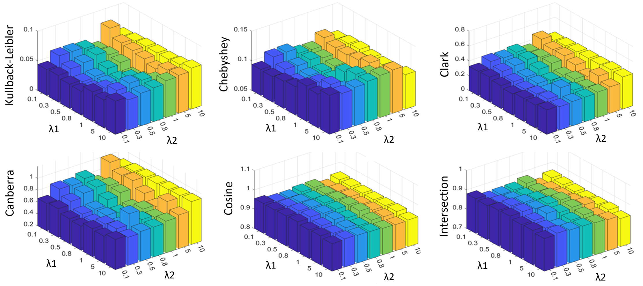
Figure 3: Influence of parameters $\lambda_{1}$ and $\lambda_{2}$ on dataset SBU-3DFE.

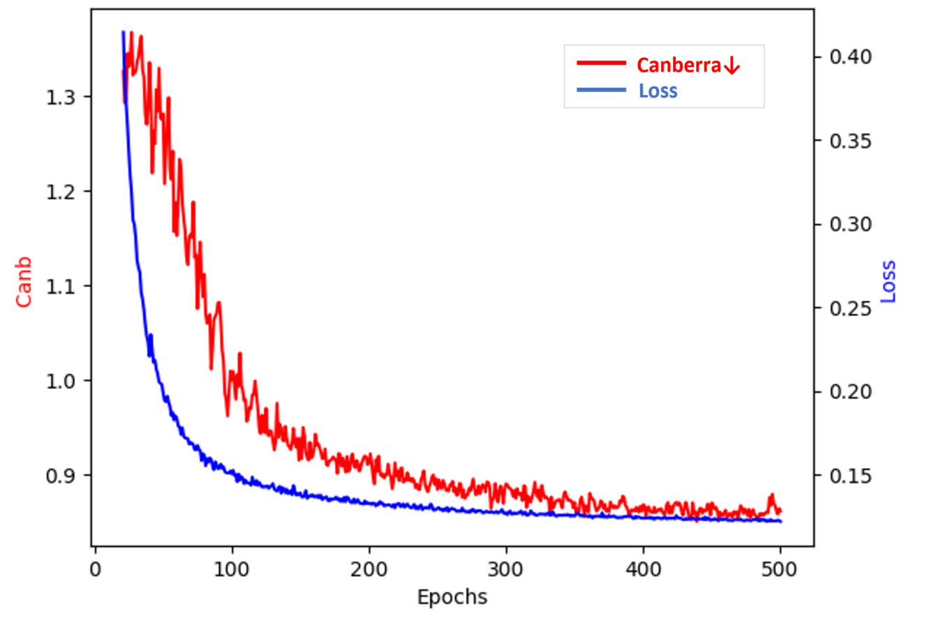
Figure 4: Convergence curve on dataset Movie.

4.4 Experimental Results

Implementation Details.

In ConLE, we adopt the SGD optimizer Ruder (2016) for optimization and utilize the LeakyReLU activation function Maas et al. (2013) to implement the networks. The code of this method is implemented by PyTorch Paszke et al. (2019) on one NVIDIA Geforce GTX 2080ti GPU with 11GB memory. All experiments for our selected comparison algorithms follow the optimal settings mentioned in their papers and we run the programs using the code provided by their relevant authors. All algorithms are evaluated by ten times ten-fold cross-validation for fairness. When comparing with other algorithms, the hyperparameters of ConLE are set as follows: $\lambda_{1}$ is set to 0.5, $\lambda_{2}$ is set to 1 and the temperature parameter $\tau_{I}$ is 0.5.

Recovery Performance.

The detailed comparison results are presented in Table 3, with the best performance on each dataset highlighted in bold. For each evaluation metric, ↓ shows the smaller the better while ↑ shows the larger the better. The average rankings of each algorithm across all the datasets are shown in the last row of each table.

The experimental results clearly indicate that our ConLE method exhibits superior recovery performance compared to the other six advanced LE algorithms. Specifically, ConLE can achieve the ranking of 1.00, 1.23, 1.00, 1.07, 1.15 and 1.00 respectively for the six evaluation metrics. ConLE obtains excellent performance both on large-scale datasets such as movie and small-scale datasets such as SJAFFE. ConLE can attain significant improvements both in comparison with algorithm adaption and specialized algorithms by exploring the description consistency of features and logical labels in the same sample. We integrate features and logical labels into the unified projection space to generate high-level features and keep the consistency of label attributes in the process of label enhancement.

Ablation Studies.

Our ConLE method consists of two main components: generating high-level features by contrastive learning and a training strategy with label-level consistency for LE. Ablation studies are conducted to verify the effectiveness of the two modules in our method.

Therefore, we first remove the part of ConLE that generates high-level features and get a comparison algorithm ConLE_h, whose loss function can be written as:

$$L_{ConLE_{h}}=\lambda_{1}l_{dis}+\lambda_{2}l_{thr},$$ (16)

In ConLE_h, we only explore the consistency information of label attributes without considering the description consistency of features and labels.

Secondly, we need to remove the strategy that ensures the consistency of label attributes. To ensure the normal training process, we still keep the strategy of minimizing the distance between label distributions and logical labels. The loss function of the comparison function ConLE_l:

$$L_{ConLE_{l}}=\lambda_{1}l_{dis}+l_{con}.$$ (17)

Table 4 provides the recovery results of ConLE_h, ConLE_l and ConLE. Due to the limitation of space, only the representative results measured on Kullback-Leibler, Clark, Canberra and Intersection are shown in the table. From the experimental results, we can observe that ConLE is superior to ConLE_h and ConLE_l in all cases. Compared with ConLE_h, ConLE considers the inherent relationship between features and logical labels. It grasps the description consistency of samples and constructs high-level features for training. Compared with ConLE_l, ConLE considers label-level consistency of logical labels and label distributions. It makes that each relevant label in the logical labels has a greater description degree in the label distributions. Therefore, our experimental results have verified that both modules of ConLE play essential roles in achieving excellent recovery performance. The integration of these modules in the complete ConLE method has been demonstrated to be highly effective.

Parameters Sensitivity.

To investigate the sensitivity of ConLE to hyperparameters, we performed experiments on SBU-3DFE with different values of the two trade-off hyperparameters $\lambda_{1}$ and $\lambda_{2}$. In this experiment, we fix one hyperparameter and choose another hyperparameter from {0.1, 0.3, 0.5, 0.8 ,1, 5, 10}. As shown in Figure 3, we can observe that the ConLE method can obtain satisfactory recovery results and our model is insensitive to $\lambda_{1}$ and $\lambda_{2}$.

Convergence Analysis.

To illustrate the convergence of ConLE, we present an experiment conducted on Movie dataset by Canberra↓ as an example, with the corresponding convergence curve depicted in Figure 4. The value of the objective function decreases and the performance increases with more iterations. Finally, they tend to be stable. The properties remain the same for all datasets.

5 Conclusion

In this work, we propose Contrastive Label Enhancement (ConLE), a novel method to cope with the (Label Enhancement) LE problem. ConLE regards features and logic labels as descriptions from different views, and then elegantly integrates them to generate high-level features by contrastive learning. Additionally, ConLE employs a training strategy that considers the consistency of label attributes to estimate the label distributions from high-level features. Experimental results on 13 datasets demonstrate its superior performance over other state-of-the-art methods.

References

- Bai et al. [2022] Junwen Bai, Shufeng Kong, and Carla P Gomes. Gaussian mixture variational autoencoder with contrastive learning for multi-label classification. In International Conference on Machine Learning, pages 1383–1398. PMLR, 2022.
- Dai and Lin [2017] Bo Dai and Dahua Lin. Contrastive learning for image captioning. Advances in Neural Information Processing Systems, 30, 2017.
- Eisen et al. [1998] Michael B Eisen, Paul T Spellman, Patrick O Brown, and David Botstein. Cluster analysis and display of genome-wide expression patterns. Proceedings of the National Academy of Sciences, 95(25):14863–14868, 1998.
- Gao et al. [2021] Yongbiao Gao, Yu Zhang, and Xin Geng. Label enhancement for label distribution learning via prior knowledge. In Proceedings of the Twenty-Ninth International Conference on International Joint Conferences on Artificial Intelligence, pages 3223–3229, 2021.
- Gao et al. [2022] Yongbiao Gao, Ke Wang, and Xin Geng. Sequential label enhancement. IEEE Transactions on Neural Networks and Learning Systems, 2022.
- Gayar et al. [2006] Neamat El Gayar, Friedhelm Schwenker, and Günther Palm. A study of the robustness of knn classifiers trained using soft labels. In IAPR Workshop on Artificial Neural Networks in Pattern Recognition, pages 67–80. Springer, 2006.
- Geng et al. [2013] Xin Geng, Chao Yin, and Zhi-Hua Zhou. Facial age estimation by learning from label distributions. IEEE transactions on pattern analysis and machine intelligence, 35(10):2401–2412, 2013.
- Geng [2016] Xin Geng. Label distribution learning. IEEE Transactions on Knowledge and Data Engineering, 28(7):1734–1748, 2016.
- Gibaja and Ventura [2014] Eva Gibaja and Sebastián Ventura. Multi-label learning: a review of the state of the art and ongoing research. Wiley Interdisciplinary Reviews: Data Mining and Knowledge Discovery, 4(6):411–444, 2014.
- Grill et al. [2020] Jean-Bastien Grill, Florian Strub, Florent Altché, Corentin Tallec, Pierre Richemond, Elena Buchatskaya, Carl Doersch, Bernardo Avila Pires, Zhaohan Guo, Mohammad Gheshlaghi Azar, et al. Bootstrap your own latent-a new approach to self-supervised learning. Advances in neural information processing systems, 33:21271–21284, 2020.
- Jiang et al. [2006] Xiufeng Jiang, Zhang Yi, and Jian Cheng Lv. Fuzzy svm with a new fuzzy membership function. Neural Computing & Applications, 15(3):268–276, 2006.
- Kanehira and Harada [2016] Atsushi Kanehira and Tatsuya Harada. Multi-label ranking from positive and unlabeled data. In Proceedings of the IEEE conference on computer vision and pattern recognition, pages 5138–5146, 2016.
- Li et al. [2015] Yu-Kun Li, Min-Ling Zhang, and Xin Geng. Leveraging implicit relative labeling-importance information for effective multi-label learning. In 2015 IEEE International Conference on Data Mining, pages 251–260. IEEE, 2015.
- Li et al. [2020] Junnan Li, Pan Zhou, Caiming Xiong, and Steven CH Hoi. Prototypical contrastive learning of unsupervised representations. arXiv preprint arXiv:2005.04966, 2020.
- Li et al. [2021] Yunfan Li, Peng Hu, Zitao Liu, Dezhong Peng, Joey Tianyi Zhou, and Xi Peng. Contrastive clustering. In Proceedings of the AAAI Conference on Artificial Intelligence, volume 35, pages 8547–8555, 2021.
- Lyons et al. [1998] Michael Lyons, Shigeru Akamatsu, Miyuki Kamachi, and Jiro Gyoba. Coding facial expressions with gabor wavelets. In Proceedings Third IEEE international conference on automatic face and gesture recognition, pages 200–205. IEEE, 1998.
- Maas et al. [2013] Andrew L Maas, Awni Y Hannun, Andrew Y Ng, et al. Rectifier nonlinearities improve neural network acoustic models. In Proc. icml, volume 30, page 3. Atlanta, Georgia, USA, 2013.
- Moyano et al. [2019] Jose M Moyano, Eva L Gibaja, Krzysztof J Cios, and Sebastián Ventura. An evolutionary approach to build ensembles of multi-label classifiers. Information Fusion, 50:168–180, 2019.
- Paszke et al. [2019] Adam Paszke, Sam Gross, Francisco Massa, Adam Lerer, James Bradbury, Gregory Chanan, Trevor Killeen, Zeming Lin, Natalia Gimelshein, Luca Antiga, et al. Pytorch: An imperative style, high-performance deep learning library. Advances in neural information processing systems, 32, 2019.
- Qi et al. [2022] Lei Qi, Jiaying Shen, Jiaqi Liu, Yinghuan Shi, and Xin Geng. Label distribution learning for generalizable multi-source person re-identification. arXiv preprint arXiv:2204.05903, 2022.
- Qian et al. [2022] Shengsheng Qian, Dizhan Xue, Quan Fang, and Changsheng Xu. Integrating multi-label contrastive learning with dual adversarial graph neural networks for cross-modal retrieval. IEEE Transactions on Pattern Analysis and Machine Intelligence, pages 1–18, 2022.
- Ruder [2016] Sebastian Ruder. An overview of gradient descent optimization algorithms. arXiv preprint arXiv:1609.04747, 2016.
- Tang et al. [2020] Haoyu Tang, Jihua Zhu, Qinghai Zheng, Jun Wang, Shanmin Pang, and Zhongyu Li. Label enhancement with sample correlations via low-rank representation. In Proceedings of the AAAI Conference on Artificial Intelligence, volume 34, pages 5932–5939, 2020.
- Wang et al. [2022] Ran Wang, Xinyu Dai, et al. Contrastive learning-enhanced nearest neighbor mechanism for multi-label text classification. In Proceedings of the 60th Annual Meeting of the Association for Computational Linguistics (Volume 2: Short Papers), pages 672–679, 2022.
- Xu et al. [2019] Ning Xu, Yun-Peng Liu, and Xin Geng. Label enhancement for label distribution learning. IEEE Transactions on Knowledge and Data Engineering, 33(4):1632–1643, 2019.
- Xu et al. [2021] N. Xu, Y. Liu, and X. Geng. Label enhancement for label distribution learning. IEEE Transactions on Knowledge; Data Engineering, 33(04):1632–1643, apr 2021.
- Xu et al. [2022] Ning Xu, Jun Shu, Renyi Zheng, Xin Geng, Deyu Meng, and Min-Ling Zhang. Variational label enhancement. IEEE Transactions on Pattern Analysis & Machine Intelligence, (01):1–15, 2022.
- Yan et al. [2016] Yan Yan, Xu-Cheng Yin, Chun Yang, Bo-Wen Zhang, and Hong-Wei Hao. Multi-label ranking with for document classification. In Chinese Conference on Pattern Recognition, pages 349–363. Springer, 2016.
- Yin et al. [2006] Lijun Yin, Xiaozhou Wei, Yi Sun, Jun Wang, and Matthew J Rosato. A 3d facial expression database for facial behavior research. In 7th international conference on automatic face and gesture recognition (FGR06), pages 211–216. IEEE, 2006.
- Zhang et al. [2015] Zhaoxiang Zhang, Mo Wang, and Xin Geng. Crowd counting in public video surveillance by label distribution learning. Neurocomputing, 166:151–163, 2015.
- Zhang et al. [2022] Shu Zhang, Ran Xu, Caiming Xiong, and Chetan Ramaiah. Use all the labels: A hierarchical multi-label contrastive learning framework. In Proceedings of the IEEE/CVF Conference on Computer Vision and Pattern Recognition, pages 16660–16669, 2022.
- Zhao et al. [2022] Xingyu Zhao, Yuexuan An, Ning Xu, and Xin Geng. Fusion label enhancement for multi-label learning. In Lud De Raedt, editor, Proceedings of the Thirty-First International Joint Conference on Artificial Intelligence, IJCAI-22, pages 3773–3779. International Joint Conferences on Artificial Intelligence Organization, 7 2022. Main Track.
- Zheng et al. [2021] Qinghai Zheng, Jihua Zhu, Haoyu Tang, Xinyuan Liu, Zhongyu Li, and Huimin Lu. Generalized label enhancement with sample correlations. IEEE Transactions on Knowledge and Data Engineering, 2021.