Long-term adherence to polytherapy in heart failure patients: a novel approach emphasising the importance of secondary prevention

Abstract

Heart failure (HF) is a severe and costly clinical syndrome associated with increased healthcare costs and a high burden of mortality and morbidity. Although drug therapy is the mainstay of treatment for heart failure, non-adherence to prescribed therapies is common and is associated with worse health outcomes and increased hospitalizations. In this study, we propose a novel approach using Latent Markov models to analyze drug adherence to polytherapy over time using a secondary database. Our methodology enables us to evaluate patients’ drug utilization behaviour, identify complex behavioural patterns, and incorporate them into predictive models to improve clinical outcomes. The significance of adhering to prescribed therapies for patients’ prognosis has been highlighted in this study. Our findings show that adherent patients gained an additional ten months of life over a seven-year follow-up period compared to non-adherent patients. This underscores the importance of secondary prevention and continuous monitoring of heart failure patients. These procedures are crucial for identifying areas of improvement and promoting better adherence to prescribed therapies.

Keywords Latent Markov Model; Polytherapy; Heart Failure; Administrative database

1 Introduction

Cardiovascular diseases represent approximately one-third of the cause of mortality worldwide, where 85% of them were due to heart attack and stroke, as stated by authoritative sources [1]. The primary goals of heart failure treatments are (i) the reduction in mortality; (ii) the prevention of recurrent hospitalization; (iii) improvement in the clinical status and functional capacity [2]. The cornerstone of HF treatment is pharmacotherapy, and the most widely administered therapies are angiotensin-converting enzyme inhibitors (ACE-I) or angiotensin-receptor blockers (ARBs) called as renin-angiotensin system (RAS), beta-blockers (BB) and mineralocorticoid receptor antagonist (MRA) [3, 4]. Guidelines suggest the use of these therapies in combination since they have been shown to reduce mortality and morbidity in heart failure patients with reduced ejection fraction [2]. Although pharmacological medicines have advanced significantly, patients with heart failure still have high mortality and hospitalization rates. One possible reason for the lack of improvement in these rates is non-adherence to prescribed therapies [5]. Multiple studies have shown that medication non-adherence is common among patients with HF, with estimated rates ranging from 10% to 93%, depending on the adherence measure used [6]. Moreover, research has revealed that patients with chronic conditions typically take around 50% of their prescribed medications [7], which has significant implications from both an epidemiological and economic perspective. Non-adherence can lead to worse patient health outcomes and an increase in hospital admissions, ultimately driving up the economic burden on the healthcare system [8, 9, 10]. Medication adherence is challenging for researchers studying heart failure because various measures are used to evaluate adherence rates [11]. Nonetheless, improving medication adherence in patients with heart failure remains crucial to enhance their health outcomes and reduce the burden on the healthcare system. Over the years, progress in understanding the pathophysiology of heart failure has led to improvements and changes in the treatments [12]. This evolution process still persists, including new pharmacological treatments such as the sodium-glucose co-transporter 2 (SGLT2) inhibitor in standard drug protocols [13]. Therefore, it is necessary to develop a methodology for analyzing adherence to polytherapy that can account for the growth of pharmacological options available for treatment over time.

Given the importance of combining therapy for treating heart failure, providing a tool capable of simultaneously describing adherence to different drugs without limiting the selected cohort is essential. Prior research has examined adherence to polytherapy [14, 15, 16], but these analyses have focused just on "user-only" patients [17]. These patients share the same indications at baseline but with different drug exposure levels, precluding the study of patients using different suggested treatments. The reasons why different therapies can be prescribed to patients with heart failure are based on various factors. Therefore, despite the guidelines suggesting mainly the use of the RAS, BB and MRA drugs, doctors’ prescriptions can be different from them based on the underlying cause of the heart failure, the severity of the condition, intolerance, and other medical conditions patients may have [2]. We are therefore interested in developing a method that non only evaluates adherence to polytherapy but can also evaluate it on a cohort of patients with different combinations of prescribed drugs.

At the same time, our interest lies in understanding the dynamics of drug adherence since, during the course of therapy, drug intake and adherence patterns can change. The disease’s progression, the patient’s health condition and their motivation to take medication can influence this evolution. Studies indicate that adherence is higher after the initial diagnosis of the disease and then tends to decline over time [18], and it has also been observed that patients typically improve their medication adherence just before and after a medical visit [19]. Initially and still today in some studies, medication adherence is modelled using binary variables without taking into account changes over time, which results in a lack of fundamental information [20]. In the available literature and current practice, several methods were developed to model this measure as a time-varying variable [21, 22]. This approach allows researchers to account for changes in adherence over time and can be an effective and accurate way to represent drug consumption.

Focusing both on the concept of polytherapy and time, in this paper, we develop an approach to model the time-varying adherence to multiple drugs. This methodology provides a description of the patient’s behaviour regarding drug utilization, capable of evaluating the temporal order of the information and capturing complex behavioural patterns which can be incorporated into current predictive models and may be associated with significant health outcomes. Motivated by the need to study the adherence to polytherapy administered to HF patients and analyze the effect on the patient’s survival probability, we proposed an innovative method to summarise time-varying adherence to polytherapy that could be used in the survival framework exploiting secondary databases.

In fact, vast amounts of health-related data have nowadays been gathered and stored in administrative healthcare databases. These databases are repositories of data collected in healthcare to let providers claim reimbursement for the health services provided [23]. The information is collected in the form of longitudinal data, that is, through repeated observations over a specific period. These databases allow access to large amounts of heterogeneous data collected systematically, which allows for the development of models based on real clinical practice [24, 25]. They reflect the real world and are particularly suitable for epidemiological research based on the study of pharmacoepidemiology. This field deals with low-frequency or long-term adverse events of drugs, requiring considerable sample sizes and extended follow-up periods [26].

This work proposes a novel procedure to analyze the longitudinal information about drug adherence provided by the administrative database using the Latent Markov models [27]. Our method is developed starting from the time-varying proportion of days covered (PDC) [28], which is an extension of the more diffuse time-fixed version [29]. Notice that one of the strengths of the method is not to limit the study only to those patients who are users of all the drugs recommended, but to manage the information about being a non-user of a drug in the modelling stage. The proposed model assumes the existence of a latent process which characterizes the patient’s behaviour concerning drug exposure, which affects the distribution of the observed (categorical) adherence to the single drugs over months in the first year of observation. We focus our attention on the most widely administered therapies to HF patients: RAS, BB and MRA. The proposed approach aims at identifying different latent states representing the willingness of patients to adhere to different drugs and investigating how behavioural change over months affects the patient’s survival probability. In addition, individuals’ demographic and health status data are used as covariates influencing the latent process. The data used in this study is taken from the Healthcare Utilisation Databases of Lombardy, a Region of Italy with approximately 16% of its population (more than 10 million residents). In particular, we refer to pharmaceutical purchases for the adherence metric construction, which provide information on the number and times of drug purchases. Since information about drug prescriptions is neither publicly available nor accessible, we approximate this information with drug purchases.

The paper is organized as follows: Chapter 2 gives an overview of the database and selected cohort while introducing the adherence metric. The methodologies used as the main contribution of this work are presented in Chapter 3, and Chapter 4 showcases the application of the methodologies to our cohort and the resulting findings. The final chapter collects the discussion of the results, highlighting their innovation and potential impact on this field.

2 Dataset

2.1 Data setting

Data from the Healthcare Utilization Databases of Lombardy, a northern region of Italy, about patients hospitalized for heart failure between 2006 and 2012 are analyzed. Information from the different databases is linked via a unique anonymous identification code to protect individual privacy. Each record in this database was associated with a hospitalization or drug purchase; hospitalization records provide information on primary diagnosis, co-existing conditions and procedures coded using the International Classification of Diseases, 9th Revision Clinical Modification (ICD-CM-9) classification system [30]. Drug purchase records code each drug according to the Anatomical Therapeutic Chemical (ATC) classification system [31], and information about the number of days of treatment covered by it is almost always extracted using the number of tablets and the Defined Daily Dose (DDD) metric [32]. However, because beta-blockers and mineralocorticoid receptor antagonists for heart failure are likely to be prescribed at lower dosages than those established for treating hypertension [33, 34], the corresponding dosage was adjusted following [35] for beta-blockers and by a working group of clinicians experts for mineralocorticoid receptor antagonist.

2.2 Cohort selection

The sample included 35,842 patients with their first HF hospital discharge between January 2006 and December 2012, excluding patients who died during the reference hospitalization. A 5 years pre-study period from 2000 to 2005 was used to consider only "incident" HF patients, that is, patients with no contact with the health care system in the previous five years due to HF. Looking at the first year of follow-up, any individual with a censoring date within this period and without any pharmacological purchase of RAS, BB and MRA was excluded. The decision to exclude them is driven by the guidelines strongly recommending therapies for decompensated patients. In addition, we were interested in analyzing drug purchases within one year of follow-up since this period allows us to observe patients’ behaviour long sufficiently to characterize them but not excessively long to limit the effect of the immortal bias. Comorbidities extracted from the ICD-9-CM codes of each hospitalization, combined with drug purchases, were used to compute the Multisource Comorbidity Score (MCS) over time for each patient [36]. This index combines hospital diagnoses and drug prescriptions to provide a tool capable of measuring the patient’s overall clinical condition and predicting the short and long-term risk of mortality.

2.3 Cumulative adherence to drugs

Medication adherence is defined by the World Health Organization as the degree to which the person’s behaviour corresponds with the agreed recommendations from a health care provider [37]. In recent years, administrative databases have been the most commonly used sources to compute adherence, so several measures were developed to calculate it. However, adherence is usually computed as a binary (or categorical) baseline covariate. One of the most used measures, according to [29] is the Proportion of Days Covered, defined as:

$$PDC=\frac{\textit{number of distinct coverage days}}{\textit{number of days in the observation period}}$$ (1)

The PDC metric is calculated during a specified period and returns a value between 0 and 1. However, in this setting, we were interested in evaluating adherence to different drugs over time since the patient’s behaviour concerning their use varies depending on their health status. Therefore, in this analysis is considered the cumulative adherence [28], which is constructed starting from the PDC as follows:

1. define a continuous time-dependent variable that indicates the cumulative months covered by drug $j$ up to time $t$ for the $i$-th patient:

   $$\texttt{com\_month}_{i}(t)=\text{distinct coverage months up to time }t$$ (2)

2. define a three levels time-dependent categorical variable that indicates the level of adherence of the $i$-th patient to the drug $j$ at time $t$:

   $$\texttt{adherence}_{i}^{(t)}=\begin{cases}0,&\text{if }\frac{\texttt{com\_month}_{i}(t)}{t}\in\text{[0, 0.25)},\\ 1,&\text{if }\frac{\texttt{com\_month}_{i}(t)}{t}\in\text{[0.25, 0.8),}\\ 2,&\text{if }\frac{\texttt{com\_month}_{i}(t)}{t}\in\text{[0.8, 1].}\\ \end{cases}$$ (3)

During the computation of the cum_month_i(t), we consider the number of distinct days covered by the prescription; this means that in case of overlapping periods, we consider the first prescription entirely and only the days of the second one not covered by the first. Adherence is calculated each month in the first year of follow-up for RAS, BB and MRA only for those patients who are users of the considered drugs, where a patient is defined as a user of a drug $j$ if purchased it at least one time in the first year after the discharge from the first heart failure hospitalization.

Calculating adherence only for users is a crucial point of our analysis since, compared to similar studies, we can manage the non-users information in the modelling phase. This means that we are able to distinguish between non-users or non-adopters patients, allowing us to understand better drug use patterns leaving out any potential biases that may arise from including data from non-users as non-adherence information.

3 Statistical Methods

3.1 Motivation for using Latent Markov Model on pharmacoepidemiology setting

Latent Markov (LM) models represent an important class of latent variable models used to analyze longitudinal data. These models study the evolution of a characteristic of interest when it is not directly observable [27]. Assume that the general behaviour of the patient about the use of drugs corresponds to the latent process. In this case, we can interpret the latent states with the patient’s levels of willingness to take the medications, which will influence the measured level of adherence. Given this perspective, this framework allows for the analysis of polytherapy intake using a unique descriptor, capable of observing the evolution of the measured adherence over time. In addition, this approach allows us to profile patients by observing the intake of different drugs simultaneously and how they change during the first year of observation.

A LM model can be seen as a latent class model [38], where patients can change latent states during the observed period. These model are an extension of the Markov chain model, which account for measurement errors [27]. In particular, the latent variable is observed with a measurement error of the response variable. Then a reasonable assumption is that the number of observable categories of the response variable is equal to the number of latent states.

LM models are based on the local independence assumption, which implies that the response variables are conditionally independent given the latent variables since the latent variables represent the unique explanatory factor of the outcomes. When it comes to therapy for heart failure patients, it is crucial to remember that the treatment plan is tailored to each individual’s needs and must be consistently followed over several months. Throughout this process, adherence is computed cumulatively, allowing us to gain valuable insights into the patient’s journey regarding drugs adherence. So, it is reasonable to assume that the latent process follows a first-order Markov chain with a certain number of states, called latent states. Essentially, the underlying therapy process can be thought of as a sequence of steps, dependent on the previous one. By identifying and understanding these latent states, we can reconstruct the path a patient takes regarding the intake of prescribed therapies.

3.2 Latent Markov Model with covariates in the latent model

In this work, we propose latent Markov models in a multivariate scenario, as our primary objective is to observe the measured adherence levels across three distinct classes of drugs. Let $J$ be the vector of the categorical response variables measured at each time occasion $t=1,...,T$. Denote $Y_{ij}^{(t)}$ the response variable $j\in{1,...,J}$ for the subject $i=1,...,n$ at time $t$, with set of categories $C_{j}$ with $c_{j}$ levels coded from $0$ to $c_{j}-1$. Take $\textbf{{Y}}_{i}^{(t)}=\left(Y_{i1}^{(t)},...,Y_{iJ}^{(t)}\right)$ as the observed multivariate response vector for the subject $i$ at time $t$ and $\widetilde{\textbf{{Y}}_{i}}=\left(\textbf{{Y}}_{i}^{(1)},...,\textbf{{Y}}_{i}^{(T)}\right)$ the relative complete response vector. Denote with $\widetilde{\textbf{{X}}_{i}}=\left(\textbf{{X}}_{i}^{(1)},...,\textbf{{X}}_{i}^{(T)}\right)$ the complete vector of all individual covariates for the subject $i$. The LMM is determined by the observed process $\widetilde{\textbf{{Y}}}_{i}$ depending on the latent process $\textbf{{U}}_{i}=\left(U_{i}^{(1)},...,U_{i}^{(T)}\right)$. The latent process follows a first-order Markov chain with state space $\{1,...,k\}$, where $k$ identifies the number of latent states. LM models usually assume that the response vectors $\textbf{{Y}}_{i}^{(t)}=\left(Y_{i1}^{(t)},...,Y_{iJ}^{(t)}\right)$ are conditionally independent given the latent process $\textbf{{U}}_{i}$ (local independence of the response vectors) and that the elements $Y_{ij}^{(t)}$ are conditionally independent given $U_{i}^{(t)}$ (conditional independence of elements).

The Latent Markov model can be seen as composed of two parts: the measurement model, which describes the conditional distribution of the response variables given the latent variables, and the latent model, which describes the distribution of the latent process. Individual covariates can be related both to the latent and the measurement model [39]. In this work, we consider only covariates affecting the initial and transition probability of the latent process. In particular, the LM model is characterized by three sets of parameters.

• The conditional response probabilities $\phi_{jy|u}^{(t)}$ is the probability of observing a response variable $y$ for variable $j$ at time $t$, given the latent state $u\in{1,...,k}$:

  $$\text{P}\left(Y^{(t)}_{ij}=y\big{|}U_{i}^{(t)}=u\right)=\phi_{jy|u}^{(t)}\qquad j=1,...,J\quad y=0,...,c_{j}-1.$$ (4)

  Define the relationship between observation and an unobserved state. If no covariates are included in the measurement model, the conditional response probabilities are time-invariant $\phi_{jy|u}^{(t)}=\phi_{jy|u}$, guaranteeing that the interpretation of the latent states remains constant over time.

• The initial state prevalence $\delta_{u|\textbf{{x}}_{i}^{(1)}}$ is the probability of being in latent state $u\in{1,...,k}$, given the vector of covariates $\textbf{{x}}_{i}^{(1)}$ for individual $i$:

  $$\text{P}\left(U_{i}^{(1)}=u\big{|}\textbf{{X}}_{i}^{(1)}=\textbf{{x}}_{i}^{(1)}\right)=\delta_{u|\textbf{{x}}_{i}^{(1)}}.$$ (5)

  The estimated $\hat{\delta}_{u|\textbf{{x}}_{i}^{(1)}}$ are proportional to the size of each latent state at the first time occasion, given the covariates. To allow initial probabilities of the latent model to depend on individual covariates, typically, is used a multinomial logit parametrization.

• The transition probabilities $\tau_{u|\bar{u}\mathbf{x}_{i}^{(t)}}^{(t)}$, represent the probability of a transition $u$ at time $t$, conditional on being in $\bar{u}$ at time $t-1$, given the individual vector of covariates $\textbf{{x}}_{i}^{(t)}$:

  $$\text{P}\left(U_{i}^{(t)}=u\big{|}U_{i}^{(t-1)}=\bar{u},\textbf{{X}}_{i}^{(t)}=\textbf{{x}}_{i}^{(t)}\right)=\tau_{u|\bar{u}\textbf{{x}}_{i}^{(t)}}^{(t)}\qquad t=2,...,T\quad u,\bar{u}=1,...,k.$$ (6)

  The estimate $\hat{\tau}_{u|\bar{u}\mathbf{x}_{i}^{(t)}}^{(t)}$ represent changes or persistence in the latent states over time given the individual covariates, also in this case, can be modelled through a multinomial logit parametrization.

When working with a latent Markov model, it is necessary to compute the marginal distribution to accurately estimate the likelihood of the observed data. By taking this approach, we can better understand the underlying patterns and relationships within the data. This distribution, also called manifest distribution, is given by:

$$\begin{split}\text{P}(\widetilde{\textbf{{y}}}_{i}\big{|}\widetilde{\textbf{{x}}}_{i})&=\text{P}\left(\widetilde{\textbf{{Y}}}_{i}=\widetilde{\textbf{{y}}}_{i}\big{|}\widetilde{\textbf{{X}}}_{i}=\widetilde{\textbf{{x}}}_{i}\right)=\\ &=\sum_{\textbf{{u}}}\text{P}\left(\widetilde{\textbf{{Y}}_{i}}=\widetilde{\textbf{{y}}_{i}}\big{|}\widetilde{\textbf{{X}}_{i}}=\widetilde{\textbf{{x}}_{i}},\textbf{{U}}_{i}=\textbf{{u}}\right)\times\text{P}\left(\textbf{{U}}_{i}=\textbf{{u}}\big{|}\widetilde{\textbf{{X}}_{i}}=\widetilde{\textbf{{x}}_{i}}\right)=\\ &=\sum_{\textbf{{u}}}\text{P}\left(\textbf{{U}}_{i}=\textbf{{u}}|\widetilde{\textbf{{X}}_{i}}=\widetilde{\textbf{{x}}_{i}}\right)\times\text{P}\left(\widetilde{\textbf{{Y}}_{i}}=\widetilde{\textbf{{y}}_{i}}\big{|}\textbf{{U}}_{i}=\textbf{{u}}\right)=\\ &=\sum_{\textbf{{u}}}\delta_{u^{(1)}|\textbf{{x}}_{i}^{(1)}}\prod_{t=2}^{T}\tau_{u^{(t)}|u^{(t-1)}\textbf{{x}}_{i}^{(t)}}^{(t)}\times\prod_{t=1}^{T}\prod_{j=1}^{J}\phi_{jy_{ij}^{(t)}|u^{(t)}}\end{split}$$ (7)

The estimation of the parameters is carried out by employing the Expectation–Maximization algorithm through the maximization of the log-likelihood for a sample on $n$ independent units [40], i.e., $\ell(\mathbf{\theta})=\sum_{i=1}^{n}\log P(\widetilde{\textbf{{y}}}_{i}\big{|}\widetilde{\textbf{{x}}}_{i})$. The algorithm’s initialization is made by applying deterministic and random initialization to reach the global maximum.

3.3 Decoding procedure

Once the model has been estimated, a decoding procedure is performed to obtain a path prediction of the latent states for each sample unit based on the data observed for this unit [27]. Two types of decoding can be applied: local decoding, which finds the most probable latent state for each time occasion, and global decoding, which finds the most probable path of latent states. This procedure is applied to the data to obtain more information on the entire latent process, which associates each patient with the longitudinal path of the states.

For each patient-specific observed data ($\widetilde{\textbf{{x}}}_{i}$, $\widetilde{\textbf{{y}}}_{i}$), the Expectation-Maximization algorithm provides the posterior probabilities of the latent state $U_{i}^{(t)}$:

$$p_{iu}^{(t)}=\text{P}\left(U_{i}^{(t)}=u\big{|}\widetilde{\textbf{{Y}}}_{i}=\widetilde{\textbf{{y}}}_{i},\widetilde{\textbf{{X}}}_{i}=\widetilde{\textbf{{x}}}_{i}\right)\qquad t=1,...,T\quad u\in{1,...,k}.$$ (8)

So, the longitudinal probability profile for the $i$-th patient, is defined as:

$$\mathbf{p}_{iu}=\left\{p_{iu}^{(t)}=P\left(U_{i}^{(t)}=u\big{|}\widetilde{\textbf{{Y}}}_{i}=\widetilde{\textbf{{y}}}_{i},\widetilde{\textbf{{X}}}_{i}=\widetilde{\textbf{{x}}}_{i}\right),\quad t=1,...,T\right\}.$$ (9)

The decoding procedure allows assigning to each patient his longitudinal profile. By reconstructing the longitudinal path, it is possible to (i) describe the patient’s adherence to therapy over months, (ii) quantify the overall adherence to polytherapy evolution over time given the patient’s history, and (iii) investigate the individual dynamic changes among latent states, detecting differences in behaviour about the drugs exposure whose effects can be analyzed in the survival framework.

4 Data application

In this section, the results obtained from the application of the proposed multivariate Latent Markov (LM) model to the Lombardy regional dataset are reported. Statistical analyses were performed in the R-software environment [41] using the LMest package [27].

4.1 Latent Markov Model for longitudinal adherence to drugs

For each month $t=1,...,12$, in the first year of observation after the first discharge for heart failure (observation period), let $\textit{J}=\{RAS,BB,MRA\}$ be the set of drugs considered, we denote with $Y_{ij}^{(t)}$ the level of adherence to the drug $j$ for each patient $i$. The relative sets of response categories identified were coded as follows:

$$C_{j}=\{0:low,1:middle,2:high\}\text{ adherence to the drug }j.$$

We considered multivariate LM models where each patient $i$ is associated with response variable $Y_{ij}$ only if it is considered user of it.

To obtain the final LM model, the first step of the procedure aims to identify the number of latent states $k$ and then select the covariates to be included in the final latent model. Basic multivariate LM models were fitted with only response variables without covariates in the latent model, increasing $k$ from 1 to 5. The number of latent states $k$ is selected according to the minimum BIC and the interpretability of the numbers of latent states. Recalling that, we are interested in classifying patients based on their adherence levels to polytherapy and then choosing a $k$ capable of synthesizing the general behaviour over the three classes of drugs considered. Once $k$ is determined, the LMM with covariates in the latent process is fitted, selecting the covariates to be included in the final model using a forward strategy. In particular, two time-fixed covariates (age and gender) and one time-varying covariate (multisource comorbidity score) were added to both the initial and transition probabilities of the latent model.

Results are shown in Table 1. The unrestricted LM model without covariates (M1) with the minimum BIC (1505148) is obtained for $k=4$, identifying a latent process with four levels of adherence. Moreover, model M2 with initial and transition probabilities parameterized by multinomial logit was preferable (BIC = 1097384) to the basic model with the same number of states. The M3-M5 models with four states and individual covariates on the latent process showed an improvement in the BIC and AIC compared to M2, and then all three covariates will be included in the final model.

Latent Markov (LM) model	k	g	$\hat{\textbf{l}}$	AIC	BIC
M1: Unrestricted LM model without covariates	1	6	-1309948	2619908	2619959
	2	35	-1100980.7	1801309	1801606
	3	86	-913655.6	1596347	1597077
	4	159	-777258.2	1503799	1505148
	5	254	-693640.8	1553876	1556031
M2: Multinomial logit LM model without covariates	4	39	-548487.7	1097053	1097384
M3: M2 + age effect on both probabilities	4	54	-548074.1	1096256	1096715
M4: M2 + gender effect on both probabilities	4	54	-548324.6	1096757	1097215
M5: M2 + time-varying MSC effect on both probabilities	4	54	-547919.2	1095946	1096405

Table 1: Results for Latent Markov (LM) model selection for longitudinal adherence to drugs with different values of latent states k and different individual covariates in the latent process. The maximum log-likelihood of each model is denoted by $\hat{l}$ and g is the number of free parameters.

The path diagram of the final model obtained combining M3-M5 models is shown in Figure 1.

• Initial probabilities were associated with the patient’s age, gender and MCS, and for each patient $i$ are defined as:

  $$\log\frac{\delta_{u|age,gender,MCS}}{\delta_{1|age,gender,MCS}}=\beta_{0u}+\beta_{1u}\cdot age_{i}+\beta_{2u}\cdot gender_{i}+\beta_{3u}\cdot MCS_{i}$$ (10)

• Transition probabilities were associated with the patient’s age, gender and MCS, and for each patient $i$ are defined as:

  $$\log\frac{\tau^{(t)}_{u|\bar{u}(age,gender,MCS)}}{\tau^{(t)}_{\bar{u}|\bar{u}(age,gender,MCS)}}=\gamma_{0\bar{u}u}+\gamma_{1\bar{u}u}\cdot age_{i}+\gamma_{2\bar{u}u}\cdot gender_{i}+\gamma_{3\bar{u}u}\cdot MCS^{(t)}_{i}$$ (11)

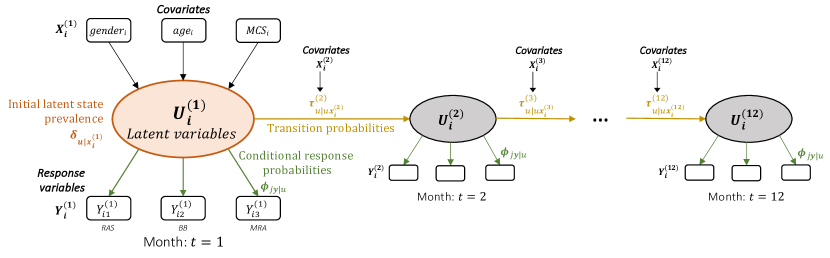
Figure 1: Path diagram for a given subject $i$ under the final Latent Markov Model with levels of adherence as response variables; age, gender and MCS as covariates affecting the initial and transition probabilities of the latent process.

Figure 2 shows the estimated conditional response probabilities $\phi_{jy|u}$ for each type of drug $y$ under the selected model. These probabilities can be useful for interpreting the latent states. Latent state 1 identifies patients with a high probability of being low-adherent to all three drugs. Patients in state 2 have a moderate level of adherence to all drugs. Patients in state 3 are highly likely to adhere to RAS and moderately to the other two drugs. Lastly, patients in state 4 have high probability to be high adherent to all three drugs. Since, in our model, the latent process features an overall measure of adherence not directly observable/measurable, we indicate this process as the level of willingness of the patients to take the prescribed drugs. With willingness, we mean the individual tendency to take drugs or to follow the medical indication about non take it, so on being non-user of the drugs. Based on this interpretation, the following states labelling was derived:

• Latent state 1: very-low willingness to be adherent to polytherapy

• Latent state 2: average willingness to be adherent to polytherapy

• Latent state 3: strong willingness to be adherent to RAS

• Latent state 4: strong willingness to be adherent to polytherapy

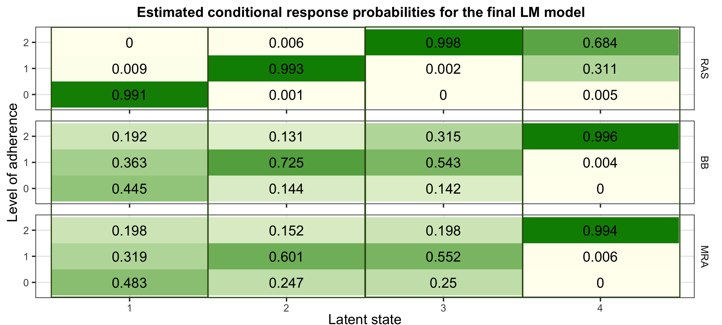
Figure 2: Estimated conditional response probabilities $\phi_{jy|u}$ for the final multivariate LM model. Each panel refers to different classes of drugs $j\in\textit{J}=\{RAS,BB,AA\}$. Each row refers to a response category $C_{j}\in\{0,1,2\}$. Each column refers to a latent state $u=\{1,2,3,4\}$.

It is important to keep in mind that the model only takes into account the therapies that have been prescribed to the patient when assessing adherence. This means that if a patient has no prescription for a specific drug, they would be classified as a non-user, and he is not be considered non-adherent to that drug. This approach ensures that the evaluation of patient adherence is based exclusively on the drugs he has to intake from clinical indications, avoiding any unnecessary penalization in evaluating overall adherence.

Regression parameters for initial probabilities
	u	2	3	4
Intercept	$\hat{\beta}_{0u}$	-0.064	-0.346***	-0.516***
Age	$\hat{\beta}_{1u}$	-0.016***	-0.002	-0.015***
GenderF	$\hat{\beta}_{2u}$	-0.080*	0.107**	0.054
MCS	$\hat{\beta}_{3u}$	-0.003	-0.010*	-0.012**

Table 2: Estimated regression parameters affecting the distribution of the initial probabilities in Equation 10.
Significance: *(%10), **(%5), ***(%1)

Table 2 displays the estimated regression parameters affecting the logit for the initial probabilities $\hat{\beta}=(\hat{\beta}_{0u},\hat{\beta}_{1u},\hat{\beta}_{2u},\hat{\beta}_{3u})$. All the estimated regression parameters affecting the logits for the initial probabilities are statistically significant. Looking at the estimates for the age, we can see that it is negative for the three states; this means that older individuals reported less adherence in the first month than younger patients. The reason for this behaviour of elderly patients can be attributed to factors such as cognitive impairment or frailty syndrome, which are often associated with old age [42]. On the other hand, the estimates for the gender female were negative only for latent state 2, indicating that female patients reported high drug adherence in the first month compared to male patients. Also, the estimates for the multisource comorbidity score are all negative, indicating that in the first month, patients with a worse condition are less adherent to drugs than patients in better clinical condition. It is important to note that patients with multiple comorbidity conditions often adhere less to therapies due to the complexity of their treatment and the potential for side effects or drug interactions [43].

Transition probabilities from $\bar{u}$ to $u$ ($\hat{\tau}_{u|\bar{u}}$)
$\bar{u}$ / $u$	1	2	3	4
1	0.825	0.165	0	0.009
2	0.021	0.895	0.058	0.027
3	0	0.051	0.936	0.013
4	0.002	0.023	0.025	0.951

Table 3: Mean estimates of the transition probabilities between latent states in Equation 11.

Table 3 shows the mean estimated transition probabilities $\hat{\tau}_{u|\hat{u}}$ between latent states. The estimated transition probabilities $\hat{\tau}_{\bar{u}|u}$ shows a high persistence in the same state, especially for latent state 3 and 4. The highest transition probability is 16.5% and is observed from state 1 to 2. Other transitions are observed from 2 to 3 (5.8%) and vice-versa (5.1%). In general, one can observe greater probabilities of increasing latent state values than decreasing values. These findings suggest that patients may face difficulty improving their adherence level once they reach a high adherence state, indicating a need for more prompt interventions to prevent a decrease in adherence. Additionally, these results emphasize the significance of regularly assessing medication adherence since patients can rapidly transition from a high to a low adherence state.

4.2 Latent-behavioural profile

Once the model parameters are estimated, the longitudinal probabilities profile $p_{iu}$ are reconstructed for each patient $i$. For each patient, we predict the longitudinal profile in the first year of observation, i.e., the sequence of latent states visited over the observation period. We evaluate the association with long-term survival for each identified longitudinal profile. Since $4^{12}$ possible pattern exists, we retained only those power by more than 1500 patients and among these, the most relevant for clinical consideration. According to this view, in Table 4, nine latent-behavioural profile may be exploited.

• A: patients assigned to the latent state 1 for all 12 months (constant level of adherence);

• B: patients assigned to the latent state 2 for all 12 months (constant level of adherence);

• C: patients assigned to the latent state 3 for all 12 months (constant level of adherence);

• D: patients assigned to the latent state 4 for all 12 months (constant level of adherence);

• E: patients who, during the 12 months, increasing of one level of latent state (i.e., of adherence);

• F: patients who, during the 12 months, increasing of two or three levels of latent state (i.e., of adherence);

• G: patients who, during the 12 months, decreasing of one level of latent state (i.e., of adherence);

• H: patients who, during the 12 months, decreasing of two or three levels of latent state (i.e., of adherence);

• I: patients with behaviour different from the previously listed (that change levels of adherence more than one time during the 12 months);

Profile	Description	n° patients
A	Always very low willingness to be adherent	1,827
B	Always average willingness to be adherent	2,601
C	Always strong willingness to be adherent to RAS	4,264
D	Always strong willingness to be adherent to polytherapy	3,767
E	Increasing one level of willingness to be adherent	8,303
F	Increasing two or three levels of willingness to be adherent	4,971
G	Decreasing one level of willingness to be adherent	4,020
H	Decreasing two or three levels of willingness to be adherent	1,958
I	Varying willingness to be adherent	4,131

Table 4: Number of patients associate with each latent-behavioural profile.

4.3 Impact of latent-behavioural profile on time-to-death event

To assess the role of the latent-behavioural profile on the overall survival time of patients, we conducted a log-rank test. The p-value of the test between the nine groups is $<2\cdot 10^{-16}$.

The comparison of survival curves between groups is shown below. Comparing patients whit the same latent state for the entire observation period (i.e. patients with four levels of adherence maintained constant over time), in Figure 3, a difference in the curves is observed. High-adherent patients have a greater probability of survival than those with moderate and very-low adherence. Patients in $C$ and $D$ groups show similar curves, with a slightly high probability of survival for those who take all drugs. These curves highlight that adherence to therapies is an important prognostic factor and that patients with higher adherence are more likely to survive than those with lower adherence, given the adjustments for age, sex and MCS. The results show that even a slight difference in adherence can significantly impact survival, emphasizing the need to educate patients on the importance of medication adherence and provide continuous support to improve their adherence. The curves highlights that patients who consistently take their prescribed medication during the observation period have a considerable gain in years of life. To quantify the adherence effect on life expectancy we implement a Restricted Mean Survival Time (RMST) analysis computing the $\Delta$RMCS [44]. The results revealed a significant positive difference in RMST between high-adherent (D) and low-adherent (A) patients. The estimate showed that patients who adhered to their prescribed therapies survived 0.831 (95%CI, [0.689, 0.973]) years longer, on average, than non-adopters when following up patients seven years.

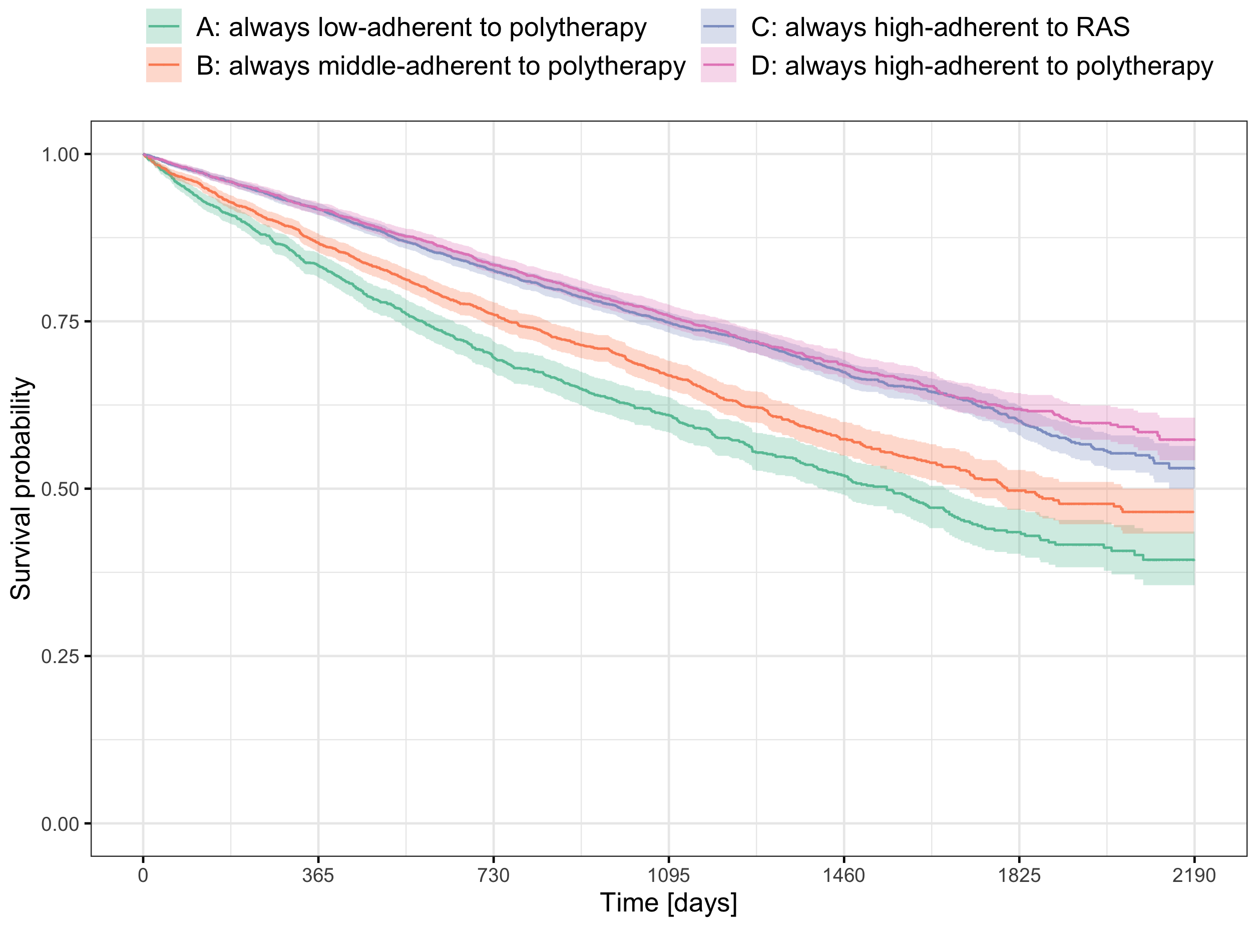
Figure 3: KM survival curves for overall survival stratified by latent-behavioural profile A, B, C and D.

In Figure 4(a), we can observe that the survival probabilities of consistently very low adherent patients are lower than those who increase their adherence over time: moving from being low-adherent to high-adherent (patients in $F$) significantly increases these probabilities. In Figure 4(b), it is possible to observe the inverse phenomenon: the probabilities of survival of patients who are always high adherent are significantly greater than those who, over time, become less adherent to the therapies. These comparisons underline the importance of analyzing the dynamics of adherence over time as it has different effects on survival curves. It highlights the need for continuous monitoring and incentives for the use of drugs, even in those patients who show low adherence in the initial period of observation. In fact, as can be seen, even those who increase over time in levels of adherence experience benefits in terms of improved health and a reduction in mortality rates. It is important to note that although adherence initially may have a positive effect on survival, inconsistent medication intake may have long-term adverse effects. This may be because heart failure requires long-term treatment to control symptoms and prevent complications. Also, discontinuation of medications can lead to a relapse of the disease and a worsening of the prognosis. Therefore, regular follow-up and interventions to improve levels of adherence should be a key focus for healthcare professionals to optimize patient outcomes and promote better medication use.

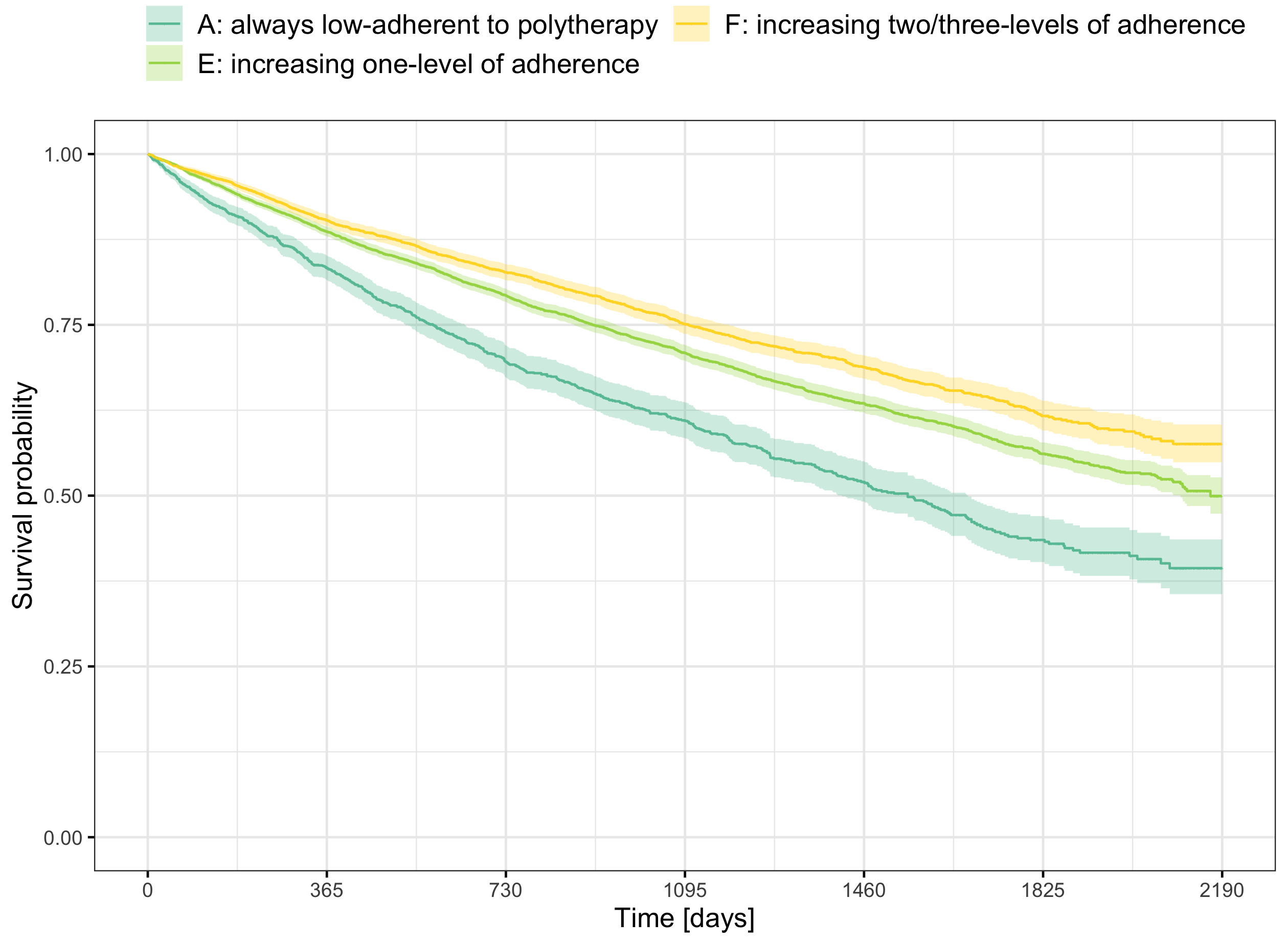
(a)

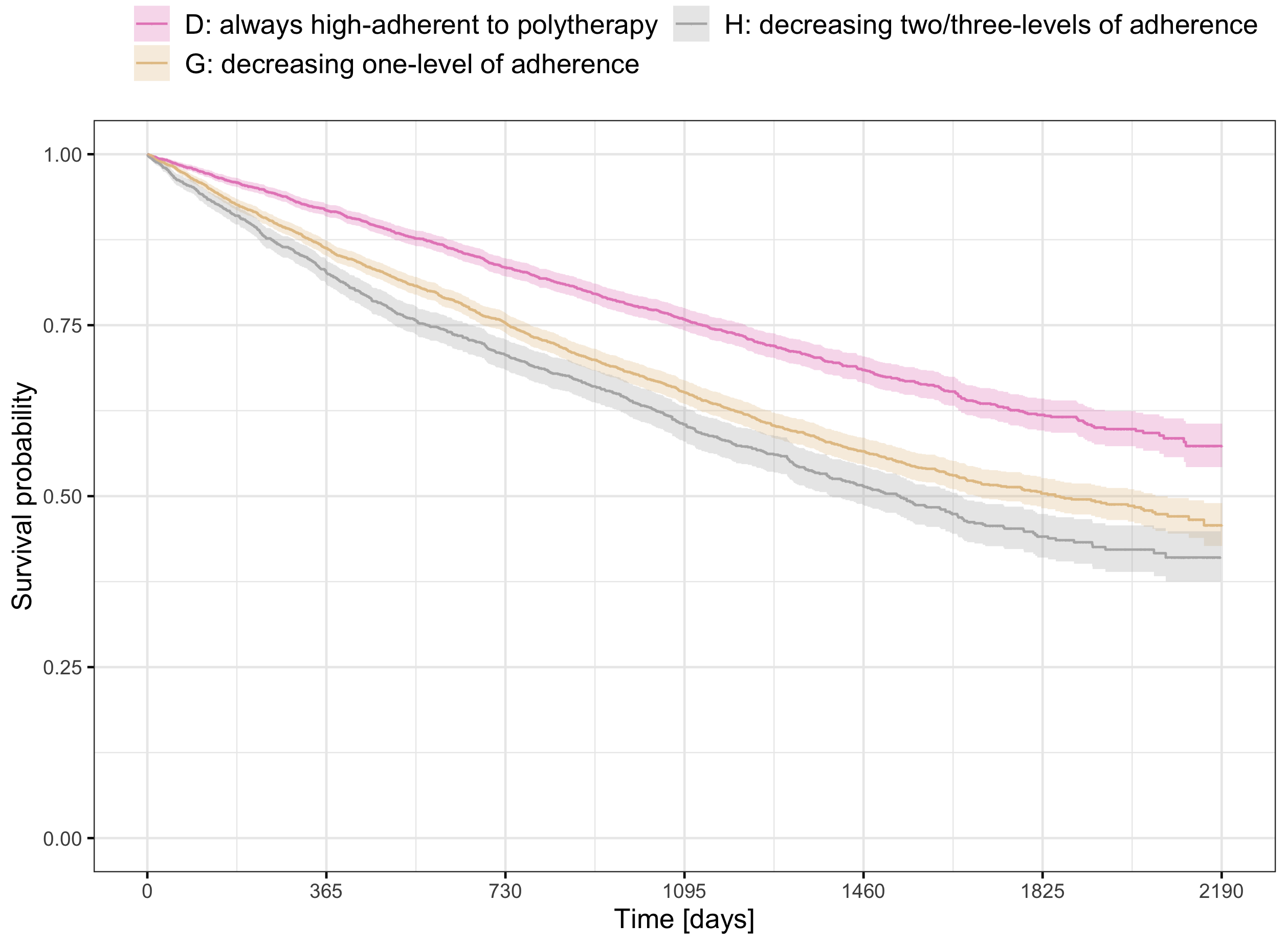
(b)

Figure 4: KM survival curves for overall survival stratified by latent-behavioural profile.

Then we perform a proportional-Hazard Cox regression model to assess the role of the available profile on the overall survival time. In addition, we added to the model other covariates such as age, gender, and MCS. The Hazard Ratios (HRs) and their 95% confidence interval obtained from the Cox model are shown in Figure 5. Seven out of eight profiles are statistically different from reference profile $A$, identifying those patients who are always low-adherent to the therapy. Being in the other profile is a protective factor for the survival probability; in particular, being in profile $C$ decreases by 43% (CI [26% - 39%]) the likelihood of death while being in $B$ by 12% (CI [2% - 20%]).

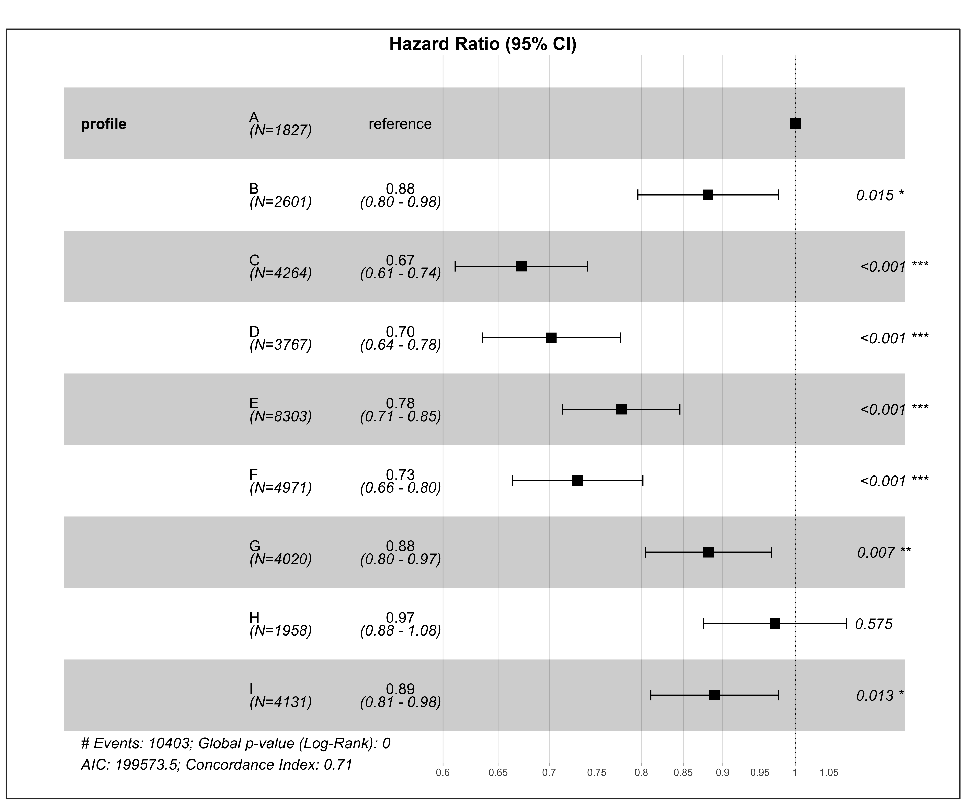
Figure 5: Hazard Ratio and its 95% confidence interval of the Cox model.

5 Discussion

We proposed an innovative study that considers the dynamic nature of drug adherence, which is often overlooked in traditional research. By utilizing an administrative database, we are able to examine the association between time-varying adherence to polytherapy and patients’ survival. The scarcity of drug adherence among heart failure patients is a significant problem, as it can significantly impact their health outcomes and quality of life. Our innovative approach to studying drug adherence allows us to understand this issue better and identify effective interventions that can improve patients’ health outcomes.

The necessity to describe complex patterns of care over time without losing the heterogeneity and variability of this information gives rise to the idea of applying the Latent Markov model to study adherence to drugs for heart failure patients. This model assumes the existence of a latent process where both its initial and transition probabilities depend on a set of individual covariates such as age, gender and the multisource comorbidity score. Since this process explains a characteristic of the observed single-adherence to drugs over time which is not directly observable, we interpret it as the willingness of the patients in taking the prescribed therapy. With willingness, we mean the individual tendency to take drugs or follow the medical indication about non-take them. This approach to defining adherence ensures that individuals who do not use specific drugs are not unfairly penalized in their evaluation of motivation to adhere to drugs. The association with a particular latent state is based only on observable information, such as computed adherence to the specific drug, which is only available for drugs the patient is considered a user of. By doing so, we can avoid confusion between being a non-user or non-adopter of therapies and allow for a more comprehensive evaluation of adherence to various therapies. Healthcare professionals can gain valuable insights from this method without restricting the cohort to "users-only". The obtained latent process is composed of four latent states, representing the different levels of the willingness: (i) people with very low motivation in taking pharmacotherapy (very-low adherence state 1), (ii) patients with middle motivation to be adherent to all drugs (average-adherence state 2), (iii) subjects with strong motivation of being adherent to RAS and middle adherent to the other two drugs (high adherence state 3), (iv) people with strong motivation to be adherent to polytherapy (very high adherence state 4).

Using an LM model to model adherence, we can create patient-specific longitudinal profiles that allow us to track the dynamic evolution of overall willingness over months for each subject. Through this process, we can identify individuals who exhibit significant patterns from a clinical perspective. The latent-behavioural profile obtained from these longitudinal profiles provides insight into how patients change their latent states over time, specifically whether they remain the same, increase, or decrease over the months. This procedure spotted nine groups of patients which captured the individual evolution of the latent process over time, showing different effects of adherence patterns on the patient’s overall survival. The results indicate that adherence to prescribed therapies is a crucial factor in a patient’s prognosis. Patients with higher adherence are more likely to survive than those with lower adherence, and monitoring and incentives for medication use are necessary for optimal outcomes. It is important to note that evaluating the persistence/change of adherence over a given period is crucial since improving or worsening individual behaviour has a different impact on the clinical state of health. Becoming adherent over time has shown positive effects on survival, while the opposite behaviour has negative effects on a patient’s health. Therefore, continuous monitoring and incentives for medication use are necessary to promote better medication use. Patients who always adhere to their medications have a significant gain in life years and a lower mortality rate. This fact is confirmed by looking at the computed years of life gained by adherent patients over the observation period, as discussed in Section 4.2, which is about ten months over seven years of follow-up. The study’s findings were slightly pessimistic compared to those obtained from randomized clinical trials, where patients are randomly assigned to receive either the treatment or a placebo and the treatment effect is estimated by comparing the outcomes of the two groups [45]. This implies that healthcare professionals must intervene early in patients who are low adherence to prescribed therapies to prevent the worsening of their medical condition and improve their survival. In addition, regular follow-up and interventions to improve levels of adherence should be a key focus for healthcare professionals to optimize patient outcomes. These improvements not only benefit patients but also have a positive impact on the healthcare system by reducing healthcare costs. Beyond evaluating the temporal evolution, this procedure evaluates the effects of different behaviours concerning the use of different therapies over time, highlighting that the risk of death decreases significantly when the patient is motivated to follow the medical indications about polytherapy. Therefore, it is essential to assess adherence to polytherapy since it can significantly impact a patient’s health and quality of life. Evaluating polytherapy adherence provides insights into medication management skills and helps identify areas for improvement, leading to better treatment plans and improved health outcomes. The significant effects of the different profiles on patients’ survival probabilities indicate that study adherence to drug combinations is prognostically relevant.

Three are the main novelties presented in this work: (i) the introduction of a new method based on Latent Markov models to summarize and quantify multiple adherence to drug and their evolution during diseases progression, where both longitudinal and categorical aspects of the observed adherence levels are included in the model; (ii) the synthesis of time-dependent information relating to the therapy using a single variable that captures the dynamic pattern of the latent process; (iii) the identification of groups of patients with a common dynamic about the overall behaviour about adherence over time allowing patients stratification which has a significant effect on patients’ survival. The developed procedure is a flexible approach that can be reproduced with a different number and types of drugs and can be adapted to other diagnostic studies.

Some limitations of the present study should also be acknowledged. The limited clinical information characterizing heart failure (i.e., ejection fraction, blood pressure) or the lack of information about contraindications/intolerance to drugs and the results of diagnostic tests are typical in this type of study, not allowing for accurate assessment of the severity of the disease. But precisely because we cannot have this detailed information that latent Markov models are even more useful since they can effectively capture the complex and dynamic nature of data and provide insights into the underlying mechanisms and factors that influence patient outcomes. Another substantial limitation of this dataset is the knowledge of the drug purchases only, instead of doses prescriptions provided by doctors. Although this information is not available in administrative databases, this study presents a significant improvement in this direction compared to others in this setting since the computation of coverage of each drug is calculated using the adjustments coefficients of the theoretical measure mainly used, the Defined Daily Dose. This adjustment of the coverage days of the drugs provides more realistic and accurate results on the computation of adherence and limits the effect of exposure misclassification. Finally, our database does not allow us to extend the analysis of the use of drugs to socioeconomic factors such as economic status, educational levels, and employment status, which are information possibly providing insights of reasons for how adherence [46]. Therefore, we could not determine if these factors play a role in the acceptance of guidelines recommending heart failure treatment with polytherapy.

6 Conclusion

This study demonstrates the importance of adherence to pharmacological therapies in the survival of patients with a chronic disease such as heart failure. The innovation of studying adherence to polytherapy, as opposed to adherence to single drugs, is particularly noteworthy, as it sheds light on medication management skills and provides valuable insights into patient behaviour. The long-term effects of drug adherence on health outcomes are crucial, as they can significantly reduce the risk of death. Therefore, it is essential to monitor patients closely regarding their therapies to identify areas for improvement and could support people in charge of the healthcare government to properly asses different patterns of care and then plan tailored patient care supporting the proper resource allocation within the National Health Service.

References

- [1] World Health Organization. Cardiovascular diseases Fact sheet reviewed June 2021. https://www.who.int/en/news-room/fact-sheets/detail/cardiovascular-diseases-(cvds), 2021. Accessed: 2023-03-27.
- [2] Theresa A. McDonagh et al. 2021 ESC guidelines for the diagnosis and treatment of acute and chronic heart failure. Eur. Heart J., 42(36):3599–3726, September 2021.
- [3] Karl Swedberg et al. Guidelines for the diagnosis and treatment of chronic heart failure: executive summary (update 2005): The Task Force for the Diagnosis and Treatment of Chronic Heart Failure of the European Society of Cardiology. European Heart Journal, 26(11):1115–1140, May 2005.
- [4] Jeffrey L. Probstfield and Kevin D. O’Brien. Progression of cardiovascular damage: The role of renin–angiotensin system blockade. The American Journal of Cardiology, 105(1, Supplement):10A–20A, 2010.
- [5] Ashley A. Fitzgerald, J. David Powers, P. Michael Ho, Thomas M. Maddox, Pamela N. Peterson, Larry A. Allen, Frederick A. Masoudi, David J. Magid, and Edward P. Havranek. Impact of medication nonadherence on hospitalizations and mortality in heart failure. Journal of Cardiac Failure, 17(8):664–669, 2011.
- [6] Jia-Rong Wu, Debra K. Moser, Terry A. Lennie, and Patricia V." Burkhart. Medication Adherence in Patients Who Have Heart Failure: a Review of the Literature. Nursing Clinics of North America, 43(1):133–53; vii–viii, 2008.
- [7] Beena Jimmy and Jimmy Jose. Patient medication adherence: measures in daily practice. Oman Med. J., 26(3):155–159, May 2011.
- [8] Scot H Simpson, Dean T Eurich, Sumit R Majumdar, Rajdeep S Padwal, Ross T Tsuyuki, Janice Varney, and Jeffrey A Johnson. A meta-analysis of the association between adherence to drug therapy and mortality. BMJ, 333(7557):15, July 2006.
- [9] P Michael Ho, Chris L Bryson, and John S Rumsfeld. Medication adherence: its importance in cardiovascular outcomes. Circulation, 119(23):3028–3035, June 2009.
- [10] Ashley A Fitzgerald, J David Powers, P Michael Ho, Thomas M Maddox, Pamela N Peterson, Larry A Allen, Frederick A Masoudi, David J Magid, and Edward P Havranek. Impact of medication nonadherence on hospitalizations and mortality in heart failure. J. Card. Fail., 17(8):664–669, August 2011.
- [11] Deval Shah, Kim Simms, Debra J Barksdale, and Jia-Rong Wu. Improving medication adherence of patients with chronic heart failure: challenges and solutions. Research Reports in Clinical Cardiology, 6:87–95, 2015.
- [12] Baek Sang Hong Kim Eui-Soon, Youn Jong-Chan. Update on the pharmacotherapy of heart failure with reduced ejection fraction. cpp, 2(4):113–133, 2020.
- [13] Shruti S Joshi, Trisha Singh, David E Newby, and Jagdeep Singh. Sodium-glucose co-transporter 2 inhibitor therapy: mechanisms of action in heart failure. Heart, 107(13):1032–1038, 2021.
- [14] Simonetta Scalvini, Palmira Bernocchi, Stefania Villa, Anna Maria Paganoni, Maria Teresa La Rovere, and Maria Frigerio. Treatment prescription, adherence, and persistence after the first hospitalization for heart failure: A population-based retrospective study on 100785 patients. International Journal of Cardiology, 330:106–111, 2021.
- [15] Marta Spreafico, Francesca Gasperoni, Giulia Barbati, Francesca Ieva, Arjuna Scagnetto, Loris Zanier, Annamaria Iorio, Gianfranco Sinagra, and Andrea Di Lenarda. Adherence to disease-modifying therapy in patients hospitalized for hf: Findings from a community-based study. American Journal of Cardiovascular Drugs, 20(2):179–190, April 2020.
- [16] Mirko Di Martino, Michela Alagna, Adele Lallo, Kendall Jamieson Gilmore, Paolo Francesconi, Francesco Profili, Salvatore Scondotto, Giovanna Fantaci, Gianluca Trifirò, Valentina Isgrò, Marina Davoli, and Danilo Fusco. Chronic polytherapy after myocardial infarction: the trade-off between hospital and community-based providers in determining adherence to medication. BMC Cardiovascular Disorders, 21(1):180, Apr 2021.
- [17] Federico Rea, Laura Savaré, Valeria Valsassina, Stefano Ciardullo, Gianluca Perseghin, Giovanni Corrao, and Giuseppe Mancia. Adherence to antidiabetic drug therapy and reduction of fatal events in elderly frail patients. Cardiovascular Diabetology, 22(1):53, March 2023.
- [18] Laura Savaré, Federico Rea, Giovanni Corrao, and Giuseppe Mancia. Use of initial and subsequent antihypertensive combination treatment in the last decade: analysis of a large italian database. Journal of Hypertension, 40(9), 2022.
- [19] P. Michael Ho, Chris L. Bryson, and John S. Rumsfeld. Medication adherence. Circulation, 119(23):3028–3035, 2009.
- [20] Susan E Andrade, Kristijan H Kahler, Feride Frech, and K Arnold Chan. Methods for evaluation of medication adherence and persistence using automated databases. Pharmacoepidemiology and drug safety, 15(8):565—74; discussion 575—7, August 2006.
- [21] Mai Alhazami, Vasco M. Pontinha, Julie A. Patterson, and David A. Holdford. Medication adherence trajectories: A systematic literature review. Journal of Managed Care & Specialty Pharmacy, 26(9):1138–1152, 2020.
- [22] Maarten J Bijlsma, Fanny Janssen, and Eelko Hak. Estimating time-varying drug adherence using electronic records: extending the proportion of days covered (PDC) method. Pharmacoepidemiol Drug Saf, 25(3):325–332, December 2015.
- [23] Calista M. Harbaugh and Jennifer N. Cooper. Administrative databases. Seminars in Pediatric Surgery, 27(6):353–360, 2018.
- [24] Cristina Mazzali, Anna Maria Paganoni, Francesca Ieva, Cristina Masella, Mauro Maistrello, Ornella Agostoni, Simonetta Scalvini, Maria Frigerio, and HF Data Project. Methodological issues on the use of administrative data in healthcare research: the case of heart failure hospitalizations in lombardy region, 2000 to 2012. BMC Health Serv. Res., 16:234, July 2016.
- [25] Daniel Timofte, Anca Pantea Stoian, et al. A review on the advantages and disadvantages of using administrative data in surgery outcome studies. The Journal of Surgery, 14, January 2018.
- [26] Natalie Gavrielov-Yusim and Michael Friger. Use of administrative medical databases in population-based research. J. Epidemiol. Community Health, 68(3):283–287, March 2014.
- [27] Francesco Bartolucci, Alessio Farcomeni, and Fulvia Pennoni. Latent Markov Models for Longitudinal Data. Chapman & Hall/CRC, Philadelphia, PA, January 2013.
- [28] Marta Spreafico and Francesca Ieva. Dynamic monitoring of the effects of adherence to medication on survival in heart failure patients: A joint modeling approach exploiting time-varying covariates. Biom. J., 63(2):305–322, February 2021.
- [29] Sudeep Karve et al. Prospective validation of eight different adherence measures for use with administrative claims data among patients with schizophrenia. Value Health, 12(6):989–995, September 2009.
- [30] Centers for Disease Control and Prevention. International Classification of Diseases, Ninth Revision, Clinical Modification (ICD-9-CM) reviewed November 2021. https://www.cdc.gov/nchs/icd/icd9cm.htm. Accessed: 2023-03-29.
- [31] World Health Organization. Anatomical Therapeutic Chemical (ATC) Classification. https://www.who.int/tools/atc-ddd-toolkit/atc-classification. Accessed: 2023-03-29.
- [32] World Health Organization. Defined Daily Dose (DDD). https://www.who.int/tools/atc-ddd-toolkit/about-ddd. Accessed: 2023-03-29.
- [33] Jeffrey J. Goldberger, Robert O. Bonow, Michael Cuffe, Alan Dyer, Yves Rosenberg, Robert O’Rourke, Prediman K. Shah, and Sidney C. Smith Jr. Beta-Blocker use following myocardial infarction: Low prevalence of evidence-based dosing. American Heart Journal, 160(3):435–442.e1, 2010.
- [34] Faiez Zannad, Wendy Gattis Stough, Patrick Rossignol, Johann Bauersachs, John J.V. McMurray, Karl Swedberg, Allan D. Struthers, Adriaan A. Voors, Luis M. Ruilope, George L. Bakris, Christopher M. O’Connor, Mihai Gheorghiade, Robert J. Mentz, Alain Cohen-Solal, Aldo P. Maggioni, Farzin Beygui, Gerasimos S. Filippatos, Ziad A. Massy, Atul Pathak, Ileana L. Piña, Hani N. Sabbah, Domenic A. Sica, Luigi Tavazzi, and Bertram Pitt. Mineralocorticoid receptor antagonists for heart failure with reduced ejection fraction: integrating evidence into clinical practice. European Heart Journal, 33(22):2782–2795, 08 2012.
- [35] Federico Rea, Raffaella Ronco, Roberto F E Pedretti, Luca Merlino, and Giovanni Corrao. Better adherence with out-of-hospital healthcare improved long-term prognosis of acute coronary syndromes: Evidence from an italian real-world investigation. Int. J. Cardiol., 318:14–20, November 2020.
- [36] Giovanni Corrao, Federico Rea, Mirko Di Martino, Rossana De Palma, et al. Developing and validating a novel multisource comorbidity score from administrative data: a large population-based cohort study from italy. BMJ Open, 7(12), 2017.
- [37] Fabienne Dobbels, Rita Van Damme-Lombaert, Johan Vanhaecke, and Sabina De Geest. Growing pains: non-adherence with the immunosuppressive regimen in adolescent transplant recipients. Pediatr. Transplant., 9(3):381–390, June 2005.
- [38] Linda M. Collins and Stephanie T. Lanza. Latent Class and Latent Transition Analysis: With Applications in the Social, Behavioral, and Health Sciences. John Wiley and Sons Inc., United States, January 2010.
- [39] Francesco Bartolucci, Monia Lupparelli, and Giorgio E. Montanari. Latent markov model for longitudinal binary data: An application to the performance evaluation of nursing homes. The Annals of Applied Statistics, 3(2):611–636, 2009.
- [40] F Bartolucci, A Farcomeni, and F Pennoni. Latent markov models: a review of a general framework for the analysis of longitudinal data with covariates. Test (Madr.), 23(3):433–465, September 2014.
- [41] R Core Team. R: A Language and Environment for Statistical Computing. R Foundation for Statistical Computing, Vienna, Austria, 2022.
- [42] Beata Jankowska-Polańska, Natalia Świątoniowska-Lonc, Agnieszka Sławuta, Dorota Krówczyńska, Krzysztof Dudek, and Grzegorz Mazur. Patient-Reported compliance in older age patients with chronic heart failure. PLoS One, 15(4), April 2020.
- [43] George J Knafl and Barbara Riegel. What puts heart failure patients at risk for poor medication adherence? Patient Prefer. Adherence, 8:1007–1018, July 2014.
- [44] Zachary R. McCaw, Guosheng Yin, and Lee-Jen Wei. Using the restricted mean survival time difference as an alternative to the hazard ratio for analyzing clinical cardiovascular studies. Circulation, 140(17):1366–1368, 2019.
- [45] Carlotta Perego, Marco Sbolli, Claudia Specchia, Mona Fiuzat, Zachary R McCaw, Marco Metra, Chiara Oriecuia, Giulia Peveri, Lee-Jen Wei, Christopher M O’Connor, and Mitchell A Psotka. Utility of restricted mean survival time analysis for heart failure clinical trial evaluation and interpretation. JACC Heart Fail., 8(12):973–983, December 2020.
- [46] G Corrao, A Zambon, A Parodi, M Mezzanzanica, L Merlino, G Cesana, and G Mancia. Do socioeconomic disparities affect accessing and keeping antihypertensive drug therapy? evidence from an italian population-based study. J. Hum. Hypertens., 23(4):238–244, April 2009.