Rethinking the editing of generative adversarial networks: a method to estimate editing vectors based on dimension reduction

Abstract

While Generative Adversarial Networks (GANs) have recently found applications in image editing, most previous GAN-based image editing methods require large-scale datasets with semantic segmentation annotations for training, only provide high level control, or merely interpolate between different images. Previous researchers have proposed EditGAN [1]for high-quality, high-precision semantic image editing with limited semantic annotations by finding ‘editing vectors’. However, it is noticed that there are many features that are not highly associated with semantics, and EditGAN [1]may fail on them. Based on the orthogonality of latent space observed by EditGAN [1], we propose a method to estimate editing vectors that do not rely on semantic segmentation nor differentiable feature estimation network. Our method assumes that there is a correlation between the intensity distribution of features and the distribution of hidden vectors, and estimates the relationship between the above distributions by sampling the feature intensity of the image corresponding to several hidden vectors. We modified Linear Discriminant Analysis (LDA) to deal with both binary feature editing and continuous feature editing. We then found that this method has a good effect in processing features such as clothing type and texture, skin color and hair.

1 Introduction

Image Editing and Manipulation.

GAN-based image editing methods can be broadly sorted into a number of categories. (i) One line of work relies on the careful dissection of the GAN’s latent space, aiming to find interpretable and disentangled latent variables, which can be leveraged for image editing, in a fully unsupervised manner [2, 3, 4, 5, 6, 7, 8, 9, 10, 11, 12, 13]. Although powerful, these approaches usually do not result in any high-precision editing capabilities. The editing vectors we are learning in EditGAN [1]would be too hard to find independently without segmentation-based guidance. (ii) Other works utilize GANs that condition on class or pixel-wise semantic segmentation labels to control synthesis and achieve editing [14, 15, 16, 17, 18, 19, 20]. Hence, these works usually rely on large annotated datasets, which are often not available, and even if available, the possible editing operations are tied to whatever labels are available. This stands in stark contrast to EditGAN [1], which can be trained in a semi-supervised fashion with very little labeled data and where an arbitrary number of high-precision edits can be learnt. (iii) Furthermore, auxiliary attribute classifiers have been used for image manipulation [21, 22], thereby still relying on annotated data and usually only providing high-level control. (iv) Image editing is often explored in the context of “interpolating” between a target and different reference image in sophisticated ways, for example by replacing certain features in a given image with features from a reference images [23, 17, 24, 25]. From the general image editing perspective, the requirement of reference images limits the broad applicability of these techniques and prevents the user from performing specific, detailed edits for which potentially no reference images are available. (v) Recently, different works proposed to directly operate in the parameter space of the GAN instead of the latent space to realize different edits [26, 6, 27]. For example, [6, 27] essentially specialize the generator network for certain images at test time to aid image embedding or “rewrite” the network to achieve desired semantic changes in output. The drawback is that such specializations prevent the model from being used in real-time on different images and with different edits. [26] proposed an approach that more directly analyses the parameter space of a GAN and treats it as a latent space in which to apply edits. However, the method still merely discovers edits in the network’s parameter space, rather than actively defining them like we do. It remains unclear whether their method can combine multiple such edits, as we can, considering that they change the GAN parameters themselves. (vi) Finally, another line of research targets primarily very high-level image and photo stylization and global appearance modifications [28, 29, 19, 20, 30, 31, 32, 33, 34].

Generally, most works only do relatively high-level and not the detailed, high-precision editing, which our model targets. Hence, we consider our model as complementary to this body of work.

GANs and Latent Space Image Embedding.

EditGAN [1]builds on top of DatasetGAN [35] and SemanticGAN [36], which proposed to jointly model images and their semantic segmentations using shared latent codes. However, these works leveraged this model design only for semi-supervised learning, not for editing. EditGAN [1]also relies on an encoder, together with optimization, to embed new images to be edited into the GAN’s latent space. This task in itself has been studied extensively in different contexts before, and we are building on these works. Previous papers studied encoder-based methods [37, 38, 39, 40, 41], used primarily optimization-based techniques [7, 42, 43, 44, 45, 46, 47, 48], and developed hybrid approaches [5, 6, 42, 49, 50].

Finally, a concurrent paper [51] shares similarities with DatasetGAN [35], on which our method builds, and explores an editing approach related to EditGAN [1]as one of its applications. However, our editing approach is methodologically different and leverages editing vectors, and also demonstrates significantly more diverse and stronger experimental results. Furthermore, [52] shares some high level ideas with EditGAN [1]; however, it leverages the CLIP [53] model and targets text-driven editing.

2 Related work

2.1 GAN and latent space image embedding

DatasetGAN [35] and SemanticGAN [36] proposed to jointly model images and their semantic segmentations using shared latent codes. For the generative adversarial network model,

$$\textnormal{Generator: }\mathcal{W^{+}}\rightarrow\mathcal{X}$$

$$\textnormal{Discriminator: }\mathcal{X}\rightarrow\mathrm{score}[0,1]$$

The generator generates pictures of image space $\mathcal{X}$ from latent space $\mathcal{W^{+}}$, while the discriminator classified the generated pictures to different label. However, these works leveraged this model design only for semi-supervised learning, not for editing.

2.2 EditGAN

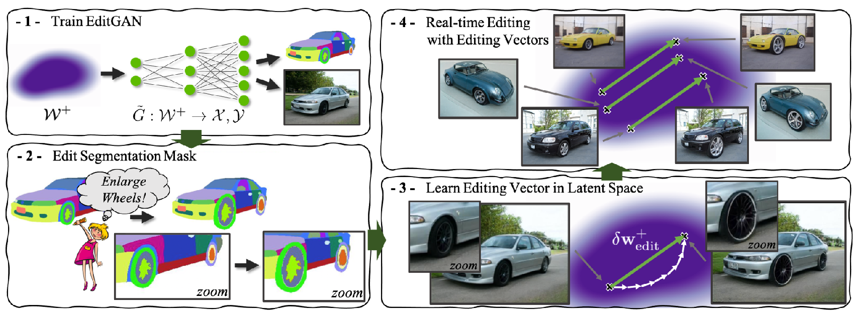
Figure 1: Pipeline of EditGAN

Our model lies in leveraging the joint distribution of images and semantic segmentation for high-precision image editing. EditGAN try to embed new image into latent space, generate the corresponding segmentation output. The new model is,

$$\textnormal{Generator: }\mathcal{W^{+}}\rightarrow\mathcal{X},\mathcal{Y}$$

$$\textnormal{Discriminator: }\mathcal{X},\mathcal{Y}\rightarrow\mathrm{score}[0,1]$$

while $\mathcal{Y}$ represents semantic space. EditGAN [1]denote the edited segmentation mask by $\mathbf{y}_{\textnormal{edited}}$. Starting from the embedding $\mathbf{w}^{+}$ of the unedited image $\mathbf{x}$ and segmentation $\mathbf{y}$, EditGAN [1]then perform optimization within $\mathcal{W}^{+}$ to find a new $\mathbf{w}^{+}_{\textnormal{edited}}=\mathbf{w}^{+}+\delta\mathbf{w}^{+}_{\textnormal{edit}}$ consistent with the new segmentation $\mathbf{y}_{\textnormal{edited}}$, while allowing the RGB output $\mathbf{x}$ to change within the editing region.

EditGAN [1]formally seeks an $editing\ vector$ $\delta\mathbf{w}_{edit}^{+}\in\mathcal{W}^{+}$ such that $(\mathbf{x}_{edited},\mathbf{y}_{edited}=\tilde{G}(\mathbf{w}^{+}+\delta\mathbf{w}_{edit}^{+})$, where $\tilde{G}$ denotes the fixed generator that synthesizes both images and segmentation. To find $\delta\mathbf{w}^{+}$, approximating $\delta\mathbf{w}_{edit}^{+}$, EditGAN [1]use the following losses as minimization targets:

$$\begin{split}\mathcal{L}_{\textnormal{RGB}}(\delta\mathbf{w}^{+})&=L_{\textnormal{LPIPS}}(\tilde{G}^{\mathbf{x}}(\mathbf{w}^{+}+\delta\mathbf{w}^{+})\odot(1-r),\mathbf{x}\odot(1-r))\\ &+L_{L2}(\tilde{G}^{\mathbf{x}}(\mathbf{w}^{+}+\delta\mathbf{w}^{+})\odot(1-r),\mathbf{x}\odot(1-r))\end{split}$$ (1)

$$\mathcal{L}_{\textnormal{CE}}(\delta\mathbf{w}^{+})=H(\tilde{G}^{\mathbf{y}}(\mathbf{w}^{+}+\delta\mathbf{w}^{+})\odot r,\mathbf{y}_{\textnormal{edited}}\odot r)$$ (2)

$$\mathcal{L}_{\textnormal{ID}}(\delta\textbf{w}^{+})=\langle R(\tilde{G}^{\textbf{x}}(\textbf{w}^{+}+\delta\textbf{w}^{+}),R(\textbf{x}))\rangle$$ (3)

where $H$ denotes the pixel-wise cross-entropy, $L_{\textnormal{LPIPS}}$ loss is base on the Learned Perception Image Patch Similarity (LPIPS) distance [54], and $L_{L2}$ is a regular pixel-wise L2 loss. $\mathcal{L}_{\textnormal{RGB}}(\delta\mathbf{w}^{+})$ ensures that the image appearance does not change $outside$ the region of interest, while $\mathcal{L}_{\textnormal{CE}}(\delta\mathbf{w}^{+})$ ensures that the target segmentation $\mathbf{y}_{\textnormal{edit}}$ is enforced $within$ the editing region. When editing human faces, EditGAN [1]also apply the identity loss $\mathcal{L}_{\textnormal{ID}}(\delta\mathbf{w}^{+})$, with $R$ denoting the pre-trained ArcFace feature extraction network and $\langle\cdot,\cdot\rangle$ cosine-similarity.

The final objective function for optimization then becomes:

$$\mathcal{L}_{\textnormal{editing}}(\delta\mathbf{w}^{+})=\lambda_{1}^{\textnormal{editing}}\mathcal{L}_{\textnormal{RGB}}(\delta\mathbf{w}^{+})+\lambda_{2}^{\textnormal{editing}}\mathcal{L}_{\textnormal{CE}}(\delta\mathbf{w}^{+})+\lambda_{3}^{\textnormal{editing}}\mathcal{L}_{\textnormal{ID}}(\delta\mathbf{w}^{+})$$ (4)

with hyper-parameters $\lambda_{1,\cdots,3}^{\textnormal{editing}}$. The only "learnable" variable is the editing vector $\delta\mathbf{w}^{+}$; all neural networks are kept fix. After optimizing $\delta\mathbf{w}^{+}$ with the objective function, we can use $\delta\mathbf{w}^{+}\approx\delta\mathbf{w}_{edit}^{+}$. EditGAN [1]rely on the generator, trained to synthesize realistic images, to modify the RGB values in the editing region in a plausible way consistent with the segmentation edit.

Summarizing, EditGAN [1]perform image editing with EditGAN [1]in three different modes:

• Real-time Editing with Editing Vectors. For localized, well-disentangled edits EditGAN [1]perform editing purely by applying previously learnt editing vectors with varying scales $s_{edit}$ and manipulate images at interactive rates.

• Vector-based Editing with Self-Supervised Refinement. For localized edits that are not perfectly disentangled with other parts of the image, we can remove editing artifacts by additional optimization at test time, while initializing the edit using the learnt editing vectors.

• Optimization-based Editing. Image-specific and very large edits do not transfer to other images via editing vectors. For such operations, EditGAN [1]perform optimization from scratch.

2.3 Shortage of EditGAN

Although EditGAN [1]pays attention to the orthogonality of latent space, it only uses this property to propose the method of editing vectors, and does not make use of the properties of space in the process of solving editing vectors.

Besides, as we have introduced above, EditGAN [1]is an optimization based approach which requires plenty handful annotations and heavy training, especially when training its semantic branch.

3 Method

3.1 Latent space analysis

InterfaceGAN [3] proposed that hyperplane can be found in latent space to classify whether the image generated by any latent vector has specific features, which inspired us to consider the relationship between the hyperplane found in latent space to classify features and the corresponding editing vector.

Given a well-trained GAN model, the generator can be viewed as a deterministric function $g:\ \mathcal{W}\rightarrow\mathcal{X}$. Here, $\mathcal{W}\in\mathbb{R}$ denotes the $d$-dimensional latent space. $\mathcal{X}$ stands for the image space, where each sample x possesses certain semantic information, like gender and age for face model. Suppose we have a semantic scoring function $f_{s}:\ \mathcal{X}\rightarrow\mathcal{S}$, where $\mathcal{S}\in\mathbb{R}^{m}$ represents the semantic space with $m$ semantics. InterfaceGAN [3] bridge the latent space $\mathcal{W}$ and the semantic space $\mathcal{S}$ with $\textbf{s}=f_{s}(g(\textbf{z}))$, where s and z denote semantic scores and the sampled latent code respectively.

Given a hyperplane with unit normal vector $\textbf{n}\in\mathbb{R}^{d}$, we define the "distance" from a sample z from lantent space to this hyperplane as

$$d(\textbf{n},\textbf{z})=\textbf{n}^{T}\textbf{z}$$ (5)

Here, $d(\cdot,\cdot)$ is not a strictly defined distance since it can be negative. When z lies near the boundary and across the hyperplane, both the "distance" and the semantic score very accordingly. Moreover, it is just when the "distance" changes its numerical sign that the semantic attribute reverses. We therefore expect these two items to be linearly dependent with

$$f(g(\textbf{z}))=\lambda d(\textbf{{n}, {z}})$$ (6)

where $f(\cdot)$ is the scoring function for a particular semantic, and $\lambda>0$ is a scalar to measure how fast the semantic varies along with the change of "distance". Random samples drawn from specific distribution are very likely to locate close enough to a given hyperplane. Therefore, the corresponding semantic can be modeled by the linear subspace that is defined by n.

One of the major differences between our case and InterfaceGAN [3] is the optimization problem. InterfaceGAN [3] uses Support Vector Machines (SVM) [55] to classify existence of feature in latent space, which is to maximize interval between two classes. In our case, the objective function is slightly different, which is to find the vector from the center of one class to another.

Another major difference is the number of annotations. InterfaceGAN [3] originally uses $6000$ fine-annotated samples (12 times of the dimension of latent space), while in we uses only $1000$ samples (2 times of the dimension of latent space). Which lead us to dimension reduction methods rather than learning base methods.

3.2 Dimension reduction in latent space

The features we deal with fall into two categories: binary features which has only two states (have or not have); continuous features which can be regarded to has strength from 0 to 1.

3.2.1 Binary feature editing

With respect to binary features, We introduced Linear Discrimination Analysis(LDA) [56] to handle binary feature. In the binary classification problem, LDA [56] can robustly estimate the projection vector that maximizes the distance between classes and minimizes the variance within a class after data points are projected.

3.2.2 Continuous features editing

Estimating editing vector for continuous features is far more tricky. Here we proposed two approaches that are bipolar method and discretizing method.

Bipolar method is to split the dataset into low, medium and high strength parts, and let the low strength part be class 0 and high strength part be class 1 to obtain estimation of editing vector. This method is quite straightforwards but not accurate nor efficient.

Discretizing method also split the dataset into parts but with more bins. Ordinarily we use a setting with $5$ groups: $[0,0.2)$, $[0.2,0.4)$, $[0.4,0.6)$, $[0.6,0.8)$ and $[0.8,1]$. Rather than performing multi-class LDA [56] to obtain a class by class discriminator, we set the optimization problem to find a single projection vector that maximize between class scatter and minimize within class scatter when projected on it. The normal form of the optimization problem is define as below:

3.2.3 Modified Linear Discriminant Analysis

Given a dataset $\mathbf{X}$ with $M$ labels, we can separate the dataset into several groups according to the labels, which is denoted as $\mathbf{X}_{i}$, where $i\in\{1,...,M\}$. In each group $\mathbf{X}_{i}$ of size $n_{i}$, we denote $x_{ij}\in\mathbb{R}^{N}$ as the data point in this group where $j\in\{1,...,n_{i}\}$ and $m_{i}$ as the group center, i.e. $m_{i}=\frac{1}{\mathbf{n_{i}}}\sum_{j}x_{ij}$. Denote $\bar{m}$ as the center of the whole dataset $\mathbf{X}$.

In order to get a good classification result, we need to maximize variance between groups $Var_{bg}$ and minimize variance in groups $Var_{ig}$ after projection. Denote $\mu\in\mathbb{R}^{N}$ as the projection vector. Hence, we can calculate both two variances.

$$Var_{bg}=\sum_{i=1}^{M}\left[\mu^{T}(m_{i}-\bar{m})\right]^{2}=\mu^{T}\left(\sum_{i=1}^{M}(m_{i}-\bar{m})(m_{i}-\bar{m})^{T}\right)\mu$$ (7)

$$Var_{ig}=\sum_{i=1}^{M}\sum_{j=1}^{n_{i}}\left[\mu^{T}(x_{ij}-m_{i})\right]^{2}=\mu^{T}\left(\sum_{i=1}^{M}\sum_{j=1}^{n_{i}}(x_{ij}-m_{i})(x_{ij}-m_{i})^{T}\right)\mu$$ (8)

For convenience, we denote $V=\sum_{i=1}^{M}\sum_{j=1}^{n_{i}}(x_{ij}-m_{i})(x_{ij}-m_{i})^{T}$ and $S=\sum_{i=1}^{M}(m_{i}-\bar{m})(m_{i}-\bar{m})^{T}$.

In order to maximize $Var_{bg}$ and minimize $Var_{ig}$ at the same time, we formulate the following optimization problem:

$$\max_{\mu}\qquad\frac{\mu^{T}V\mu}{\mu^{T}S\mu}$$ (9)

It is trivial to see that (9) is equivalent to the following:

$$\begin{aligned} \max_{\mu}&\qquad\mu^{T}V\mu\\ \mathrm{s.t.}&\qquad\mu^{T}S\mu=1.\end{aligned}$$ (10)

By applying Lagrange multipliers, we could define the Lagrange function $L$:

$$L=\mu^{T}V\mu-\lambda(\mu^{T}S\mu-1)$$ (11)

According to the KKT conditions, we could get the optimal value is the biggest eigenvector $\lambda_{1}$ of $S^{-1}V$ and the corresponding solution $\mu^{*}$ is the corresponding eigenvector of $\lambda_{1}$.

Noting that $S$ may not be invertible, which could block the calculation. We could use some technique to avoid this situation. Denote $\epsilon$ as a small number and $I\in\mathbb{R}^{N\times N}$ as the identity matrix. We add $\epsilon I$ to $S$ to keep the new $S$ invertible.

4 Experiments

As GAN based editing methods require a well-trained GAN network as base model, we choose StyleGAN-Human as our base GAN model.

4.1 EditGAN methods

According to the method of EditGAN [1], we manually labeled 100 groups of human body segmentation data, trained semantic branches, and then obtained the editing vectors of the upper garment lengths. The editing results by vectors obtained by EditGAN [1]methods are shown in Fig 2.

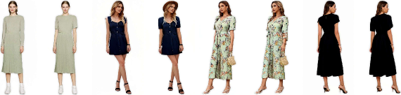
Figure 2: Editing results of EditGAN [1]methods.

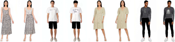
Figure 3: Editing results of binary feature

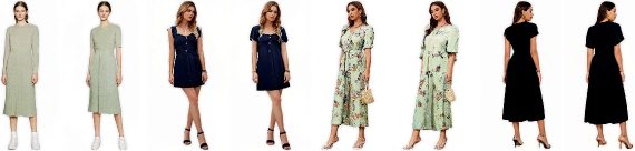
Figure 4: Editing results of continuous feature

Table 1: Cross validation results between EditGAN and ours

Metrics	EditGAN[1]	Ours
Correlation	0.5788	0.3911
L2 distance	1.1214

4.2 Proposed methods

Binary feature editing

We set whether there is pattern on cloth as the target feature and labeled 500 images. According to the method discussed above, we perform LDA [56] over the sample sets and obtain the editing vector. The editing results are shown in Fig 3.

Continuous feature editing

We use the length of upper garment as target feature to compare with EditGAN [1]method and labeled 500 images. Then the discretizing method was performed according to the method discussed above to obtain the editing vector. The editing results are shown in Fig 4.

4.3 Cross validation

As both methods estimate the editing vector for length of upper garment, it is possible to compare their effectiveness on feature strength estimation and consistency. We compared the correlation between projection length and feature strength and the L2 distance between two editing vector. The results are shown in Table 1.

5 Conclusion

We have developed an efficient GAN image editing technology based on the vector space editing technology proposed by EditGAN [1], and proved that our method can efficiently find the general direction of the editing vector under its limited annotation data. Compared with EditGAN [1], our method explicitly has the ability to edit discrete binomial features; Compared with InterfaceGAN [3], our method proposes an efficient method to find edit vectors on continuous features. At the same time, we noticed that the editing vector we found was not completely decoupled from other features, and some other features also changed in the editing process. In the future, we plan to explore more explicit editing vector estimation methods on continuous features. We also plan to better solve the decoupling problem of editing vectors in finite annotation.

6 Contribution percent

Haoran Jiang: 20%

Qi Li: 20%

Xuyang Li: 20%

Yuhan Cao: 20%

Zhenghong Yu: 20%

References

- [1] H. Ling, K. Kreis, D. Li, S. W. Kim, A. Torralba, and S. Fidler, “Editgan: High-precision semantic image editing,” in Advances in Neural Information Processing Systems (NeurIPS), 2021.
- [2] Y. Shen, J. Gu, X. Tang, and B. Zhou, “Interpreting the latent space of gans for semantic face editing,” in Proceedings of the IEEE/CVF conference on computer vision and pattern recognition, 2020, pp. 9243–9252.
- [3] Y. Shen, C. Yang, X. Tang, and B. Zhou, “Interfacegan: Interpreting the disentangled face representation learned by gans,” IEEE transactions on pattern analysis and machine intelligence, 2020.
- [4] Y. Alharbi and P. Wonka, “Disentangled image generation through structured noise injection,” in Proceedings of the IEEE/CVF Conference on Computer Vision and Pattern Recognition, 2020, pp. 5134–5142.
- [5] D. Bau, J.-Y. Zhu, H. Strobelt, B. Zhou, J. B. Tenenbaum, W. T. Freeman, and A. Torralba, “Gan dissection: Visualizing and understanding generative adversarial networks,” arXiv preprint arXiv:1811.10597, 2018.
- [6] D. Bau, H. Strobelt, W. Peebles, J. Wulff, B. Zhou, J.-Y. Zhu, and A. Torralba, “Semantic photo manipulation with a generative image prior,” arXiv preprint arXiv:2005.07727, 2020.
- [7] A. Plumerault, H. L. Borgne, and C. Hudelot, “Controlling generative models with continuous factors of variations,” arXiv preprint arXiv:2001.10238, 2020.
- [8] E. Härkönen, A. Hertzmann, J. Lehtinen, and S. Paris, “Ganspace: Discovering interpretable gan controls,” Advances in Neural Information Processing Systems, vol. 33, pp. 9841–9850, 2020.
- [9] L. Goetschalckx, A. Andonian, A. Oliva, and P. Isola, “Ganalyze: Toward visual definitions of cognitive image properties,” in Proceedings of the IEEE/CVF International Conference on Computer Vision, 2019, pp. 5744–5753.
- [10] A. Jahanian, L. Chai, and P. Isola, “On the" steerability" of generative adversarial networks,” arXiv preprint arXiv:1907.07171, 2019.
- [11] A. Voynov and A. Babenko, “Unsupervised discovery of interpretable directions in the gan latent space,” in International conference on machine learning. PMLR, 2020, pp. 9786–9796.
- [12] B. Wang and C. R. Ponce, “The geometry of deep generative image models and its applications,” arXiv preprint arXiv:2101.06006, 2021.
- [13] Y. Shen and B. Zhou, “Closed-form factorization of latent semantics in gans,” in Proceedings of the IEEE/CVF Conference on Computer Vision and Pattern Recognition, 2021, pp. 1532–1540.
- [14] Y. Choi, M. Choi, M. Kim, J.-W. Ha, S. Kim, and J. Choo, “Stargan: Unified generative adversarial networks for multi-domain image-to-image translation,” in Proceedings of the IEEE conference on computer vision and pattern recognition, 2018, pp. 8789–8797.
- [15] C.-H. Lee, Z. Liu, L. Wu, and P. Luo, “Maskgan: Towards diverse and interactive facial image manipulation,” in Proceedings of the IEEE/CVF Conference on Computer Vision and Pattern Recognition, 2020, pp. 5549–5558.
- [16] R. Wu, G. Zhang, S. Lu, and T. Chen, “Cascade ef-gan: Progressive facial expression editing with local focuses,” in Proceedings of the IEEE/CVF Conference on Computer Vision and Pattern Recognition, 2020, pp. 5021–5030.
- [17] P. Zhu, R. Abdal, Y. Qin, and P. Wonka, “Sean: Image synthesis with semantic region-adaptive normalization,” in Proceedings of the IEEE/CVF Conference on Computer Vision and Pattern Recognition, 2020, pp. 5104–5113.
- [18] S.-Y. Chen, W. Su, L. Gao, S. Xia, and H. Fu, “Deepfacedrawing: Deep generation of face images from sketches,” ACM Transactions on Graphics (TOG), vol. 39, no. 4, pp. 72–1, 2020.
- [19] T. Park, M.-Y. Liu, T.-C. Wang, and J.-Y. Zhu, “Semantic image synthesis with spatially-adaptive normalization,” in Proceedings of the IEEE/CVF conference on computer vision and pattern recognition, 2019, pp. 2337–2346.
- [20] T.-C. Wang, M.-Y. Liu, J.-Y. Zhu, A. Tao, J. Kautz, and B. Catanzaro, “High-resolution image synthesis and semantic manipulation with conditional gans,” in Proceedings of the IEEE conference on computer vision and pattern recognition, 2018, pp. 8798–8807.
- [21] X. Hou, X. Zhang, H. Liang, L. Shen, Z. Lai, and J. Wan, “Guidedstyle: Attribute knowledge guided style manipulation for semantic face editing,” Neural Networks, vol. 145, pp. 209–220, 2022.
- [22] Z. He, W. Zuo, M. Kan, S. Shan, and X. Chen, “Attgan: Facial attribute editing by only changing what you want,” IEEE transactions on image processing, vol. 28, no. 11, pp. 5464–5478, 2019.
- [23] E. Collins, R. Bala, B. Price, and S. Susstrunk, “Editing in style: Uncovering the local semantics of gans,” in Proceedings of the IEEE/CVF Conference on Computer Vision and Pattern Recognition, 2020, pp. 5771–5780.
- [24] K. M. Lewis, S. Varadharajan, and I. Kemelmacher-Shlizerman, “Vogue: Try-on by stylegan interpolation optimization,” 2021.
- [25] H. Kim, Y. Choi, J. Kim, S. Yoo, and Y. Uh, “Exploiting spatial dimensions of latent in gan for real-time image editing,” in Proceedings of the IEEE/CVF Conference on Computer Vision and Pattern Recognition, 2021, pp. 852–861.
- [26] A. Cherepkov, A. Voynov, and A. Babenko, “Navigating the gan parameter space for semantic image editing,” in Proceedings of the IEEE/CVF conference on computer vision and pattern recognition, 2021, pp. 3671–3680.
- [27] D. Bau, S. Liu, T. Wang, J.-Y. Zhu, and A. Torralba, “Rewriting a deep generative model,” in European conference on computer vision. Springer, 2020, pp. 351–369.
- [28] L. A. Gatys, A. S. Ecker, and M. Bethge, “Image style transfer using convolutional neural networks,” in Proceedings of the IEEE conference on computer vision and pattern recognition, 2016, pp. 2414–2423.
- [29] T. Park, J.-Y. Zhu, O. Wang, J. Lu, E. Shechtman, A. Efros, and R. Zhang, “Swapping autoencoder for deep image manipulation,” Advances in Neural Information Processing Systems, vol. 33, pp. 7198–7211, 2020.
- [30] F. Luan, S. Paris, E. Shechtman, and K. Bala, “Deep photo style transfer,” in Proceedings of the IEEE conference on computer vision and pattern recognition, 2017, pp. 4990–4998.
- [31] M.-Y. Liu, T. Breuel, and J. Kautz, “Unsupervised image-to-image translation networks,” Advances in neural information processing systems, vol. 30, 2017.
- [32] Y. Li, M.-Y. Liu, X. Li, M.-H. Yang, and J. Kautz, “A closed-form solution to photorealistic image stylization,” in Proceedings of the European Conference on Computer Vision (ECCV), 2018, pp. 453–468.
- [33] H. Kazemi, S. M. Iranmanesh, and N. Nasrabadi, “Style and content disentanglement in generative adversarial networks,” in 2019 IEEE Winter Conference on Applications of Computer Vision (WACV). IEEE, 2019, pp. 848–856.
- [34] J. Yoo, Y. Uh, S. Chun, B. Kang, and J.-W. Ha, “Photorealistic style transfer via wavelet transforms,” in Proceedings of the IEEE/CVF International Conference on Computer Vision, 2019, pp. 9036–9045.
- [35] Y. Zhang, H. Ling, J. Gao, K. Yin, J.-F. Lafleche, A. Barriuso, A. Torralba, and S. Fidler, “Datasetgan: Efficient labeled data factory with minimal human effort,” in Proceedings of the IEEE/CVF Conference on Computer Vision and Pattern Recognition, 2021, pp. 10 145–10 155.
- [36] D. Li, J. Yang, K. Kreis, A. Torralba, and S. Fidler, “Semantic segmentation with generative models: Semi-supervised learning and strong out-of-domain generalization,” in Proceedings of the IEEE/CVF Conference on Computer Vision and Pattern Recognition, 2021, pp. 8300–8311.
- [37] G. Perarnau, J. Van De Weijer, B. Raducanu, and J. M. Álvarez, “Invertible conditional gans for image editing,” arXiv preprint arXiv:1611.06355, 2016.
- [38] J. Donahue, P. Krähenbühl, and T. Darrell, “Adversarial feature learning,” arXiv preprint arXiv:1605.09782, 2016.
- [39] A. Brock, T. Lim, J. M. Ritchie, and N. Weston, “Neural photo editing with introspective adversarial networks,” arXiv preprint arXiv:1609.07093, 2016.
- [40] V. Dumoulin, I. Belghazi, B. Poole, O. Mastropietro, A. Lamb, M. Arjovsky, and A. Courville, “Adversarially learned inference,” arXiv preprint arXiv:1606.00704, 2016.
- [41] E. Richardson, Y. Alaluf, O. Patashnik, Y. Nitzan, Y. Azar, S. Shapiro, and D. Cohen-Or, “Encoding in style: a stylegan encoder for image-to-image translation,” in Proceedings of the IEEE/CVF conference on computer vision and pattern recognition, 2021, pp. 2287–2296.
- [42] J.-Y. Zhu, P. Krähenbühl, E. Shechtman, and A. A. Efros, “Generative visual manipulation on the natural image manifold,” in European conference on computer vision. Springer, 2016, pp. 597–613.
- [43] R. A. Yeh, C. Chen, T. Yian Lim, A. G. Schwing, M. Hasegawa-Johnson, and M. N. Do, “Semantic image inpainting with deep generative models,” in Proceedings of the IEEE conference on computer vision and pattern recognition, 2017, pp. 5485–5493.
- [44] Z. C. Lipton and S. Tripathi, “Precise recovery of latent vectors from generative adversarial networks,” arXiv preprint arXiv:1702.04782, 2017.
- [45] R. Abdal, Y. Qin, and P. Wonka, “Image2stylegan: How to embed images into the stylegan latent space?” in Proceedings of the IEEE/CVF International Conference on Computer Vision, 2019, pp. 4432–4441.
- [46] M. Huh, R. Zhang, J.-Y. Zhu, S. Paris, and A. Hertzmann, “Transforming and projecting images into class-conditional generative networks,” in European Conference on Computer Vision. Springer, 2020, pp. 17–34.
- [47] A. Creswell and A. A. Bharath, “Inverting the generator of a generative adversarial network,” IEEE transactions on neural networks and learning systems, vol. 30, no. 7, pp. 1967–1974, 2018.
- [48] A. Raj, Y. Li, and Y. Bresler, “Gan-based projector for faster recovery with convergence guarantees in linear inverse problems,” in Proceedings of the IEEE/CVF International Conference on Computer Vision, 2019, pp. 5602–5611.
- [49] D. Bau, J.-Y. Zhu, J. Wulff, W. Peebles, H. Strobelt, B. Zhou, and A. Torralba, “Seeing what a gan cannot generate,” in Proceedings of the IEEE/CVF International Conference on Computer Vision, 2019, pp. 4502–4511.
- [50] J. Zhu, Y. Shen, D. Zhao, and B. Zhou, “In-domain gan inversion for real image editing,” in European conference on computer vision. Springer, 2020, pp. 592–608.
- [51] J. Xu and C. Zheng, “Linear semantics in generative adversarial networks,” in Proceedings of the IEEE/CVF Conference on Computer Vision and Pattern Recognition, 2021, pp. 9351–9360.
- [52] D. Bau, A. Andonian, A. Cui, Y. Park, A. Jahanian, A. Oliva, and A. Torralba, “Paint by word,” arXiv preprint arXiv:2103.10951, 2021.
- [53] A. Radford, J. W. Kim, C. Hallacy, A. Ramesh, G. Goh, S. Agarwal, G. Sastry, A. Askell, P. Mishkin, J. Clark et al., “Learning transferable visual models from natural language supervision,” in International Conference on Machine Learning. PMLR, 2021, pp. 8748–8763.
- [54] R. Zhang, P. Isola, A. A. Efros, E. Shechtman, and O. Wang, “The unreasonable effectiveness of deep features as a perceptual metric,” in Proceedings of the IEEE conference on computer vision and pattern recognition, 2018, pp. 586–595.
- [55] C. Cortes and V. Vapnik, “Support vector machine,” Machine learning, vol. 20, no. 3, pp. 273–297, 1995.
- [56] R. H. Riffenburgh, “Linear discriminant analysis,” Ph.D. dissertation, Virginia Polytechnic Institute, 1957.