Towards a finite volume discretization of the atmospheric surface layer consistent with physical theory

Abstract

We study an atmospheric column and its discretization. Because of numerical considerations, the column must be divided into two parts: (1) a surface layer, excluded from the computational domain and parameterized, and (2) the rest of the column, which reacts more slowly to variations in surface conditions. A usual practice in atmospheric models is to parameterize the surface layer without excluding it from the computational domain, leading to possible consistency issues. We propose here to unify the two representations in a Finite Volume discretization. In order to do so, the reconstruction inside the first grid cell is performed using the particular functions involved in the parameterizations and not only with polynomials. Using a consistency criterion, surface layer management strategies are compared in different physical situations.

1 Introduction

A common difficulty for atmospheric models is to represent the surface layer (SL), i.e. the area directly and almost instantaneously influenced by the presence of the ground or the ocean. The scales in the SL (approximately the first 10 meters of the air column) are so small that the resolution needed for a numerical model to represent the phenomena correctly is out of reach. However, the Monin-Obukhov (MO) theory, which generalises the wall law to density-stratified fluids, provides under certain simple hypotheses (quasi-stationarity, horizontal homogeneity, etc.) an analytical formulation of the solution in the SL and the expression of the fluxes (heat, momentum) exchanged with the atmosphere above it. At the discrete level, the present treatment of this SL in numerical models is inconsistent: it is both treated like the rest of the atmosphere column by a standard numerical scheme (polynomial profile) when discretising the equations, and in a parameterised form (MO profile, which is a perturbation of a logarithmic profile, see e.g. [1]) for the calculation of fluxes. The consequences of this inconsistency are still poorly assessed in the context of atmospheric modeling, but we can mention for instance that in the context of combustion, it is mentioned in [2] that the way the wall law is implemented in a given code and the way it interacts with the numerical methods used (in particular the turbulence scheme) can influence the numerical results as much as a particular choice of wall law. In this paper, we will address this inconsistency and propose a new finite volume formulation to remedy it.

The turbulent Ekman layer model

Our approach is derived hereafter in the case of the 1D vertical Ekman layer model [3] in the neutral case. It includes the Coriolis effect with a constant parameter $f$ and a vertical turbulent flux term $\langle w^{\prime}u^{\prime}\rangle$:

$$\partial_{t}u+ifu+\partial_{z}\langle w^{\prime}u^{\prime}\rangle=ifu_{G}$$ (1)

where $i$ is the imaginary unit. The constant nudging term $u_{G}$ pulls the solution towards the geostrophic equilibrium (a large-scale solution where the pressure gradient balances the Coriolis force). The horizontal wind $u$ (in ${\rm m}.{\rm s}^{-1}$) is a complex variable accounting for both orientation and speed of the wind. The so-called Boussinesq hypothesis states that the turbulent flux is proportional to the gradient of $u$: $\langle w^{\prime}u^{\prime}\rangle=-K_{u}\partial_{z}u$ where $K_{u}\geq 0$ is the turbulent viscosity. In the SL, the MO theory states that this turbulent flux is constant along the vertical axis and provides its analytical expression. We thus obtain the system of equations given in Fig. 1.

Figure 1: Continuous equations in the computational domain $(\delta_{\rm a}, +\infty)$ and constant flux in the SL $(0,\delta_{\rm a})$. The MO theory specifies the complex constant $u_{\star}e_{\tau}$ and a range of possible values for $\delta_{\rm a}$.

Usual approach in atmospheric models.

The usual choice made in current atmospheric models is to consider that the SL extends from the wall to the center of the first cell (let us note $z_{1/2}$ this altitude). In practice this means that compatibility constraints should apply at $z=z_{1/2}$ to correctly connect the profile as parameterized in the SL with the upper profile obtained using the numerical model. However the usual practice is to integrate the region $z\leq z_{1/2}$ corresponding to the SL into the computational domain and then use the MO parameterization only to predict a surface flux at $z=0$. The impact of this approximation is poorly documented to date: (i) the extent of the SL is fixed for purely numerical reasons and not for physical reasons, which does not guarantee that the solution will converge with the resolution; (ii) the solution in the area $z\leq z_{1/2}$ is both parameterized and computed by the model, without ensuring the consistency of these two profiles. The coupling between the SL and the rest of the model is thus weak: the model provides the flow information at $z=z_{1/2}$ to the SL scheme and the latter provides in exchange a surface flux to the model at $z=0$. In general no other interaction exists. For example, with this kind of coupling, the SL structures cannot really interact with the rest of the flow. For more details and numerous references, see [4].

A few studies address this issue: several alternatives for implementing a wall law in a Large Eddy Simulation solver are proposed in [2]; a first step toward a proper Finite Volume (FV) approach is proposed by [5], where the authors extend the SL to the entire first cell $(0,z_{1})$ and design a scheme adapted to FV.

In this paper, we propose to implement directly in the FV discretization the existing assumptions underlying the MO theory. In order to do so, the reconstruction inside the first grid cell is performed using the analytical functions involved in the wall laws and not only with polynomials. This approach also allows to relax the artificial assumption $\delta_{a}=z_{1/2}$ and to extend the height of the SL beyond the first grid point if necessary (note that the log-layer mismatch, a well known numerical problem in Large Eddy Simulations, comes from a too thin SL). By being able to choose the thickness of the SL based on physical — and not only numerical — criteria, the consistency of the schemes is improved. The vertical resolution can thus be refined without changing the continuous equations solved by the discretization, thus answering the issues raised in [6]. Numerical experiments with a 1D Ekman layer model are performed, and SL management strategies are compared for different types of stratification.

2 The Finite Volume scheme

Figure 2: Summary of the notations related to the discretisation.

Spline reconstruction of solutions.

The space domain is divided into $M$ cells delimited by heights $(z_{0}=0,\ldots,z_{m},\ldots,z_{M})$. The size of the $m$-th cell is $h_{m+\frac{1}{2}}=z_{m+1}-z_{m}$ and the average of $u(z)$ over this cell is noted $\overline{u}_{m+\frac{1}{2}}=\frac{1}{h_{m+\frac{1}{2}}}\int_{z_{m}}^{z_{m+1}}u(z)dz$. The space derivative of $u$ at $z_{m}$ is noted $\phi_{m}$. Fig. 2 summarizes these notations. Averaging the evolution equation over a cell gives the semi-discrete equation

$$(\partial_{t}+if)\overline{u}_{m+\frac{1}{2}}-\frac{K_{u,m+1}\phi_{m+1}-K_{u,m}\phi_{m}}{h_{m+\frac{1}{2}}}=ifu_{G}$$ (2)

The reconstruction of $u(z)={\cal S}_{m+\frac{1}{2}}(z-z_{m+\frac{1}{2}})$ is chosen to be a quadratic polynomial (higher order schemes can be similarly derived, see [1]). The continuity of $u(z)$ and its space derivative $\phi$ between cells yields the relation:

$$\frac{h_{m-1/2}}{{6}}\phi_{m-1}+\frac{h_{m+1/2}+h_{m-1/2}}{{3}}\phi_{m}+\frac{h_{m+1/2}}{{6}}\phi_{m+1}=\bar{u}_{m+\frac{1}{2}}-\bar{u}_{m-\frac{1}{2}}$$ (3)

which is a FV approximation used in fourth-order compact schemes for the first derivative $\partial_{z}u$ and second-order for $\partial_{z}^{2}u$ (e.g. [7]).

Usual treatment of the SL with Finite Volume methods.

The typical treatment of the SL in atmospheric models is to use the evolution equation in the first cell $(z_{0},z_{1})$ to compute $\overline{u}_{\frac{1}{2}}$ and then assume that this averaged value is the wind speed at the center of the cell in the Monin-Obukhov theory applied with $\delta_{a}=z_{1}$. The corresponding bottom boundary condition is then

$$\underbrace{K_{u,0}{\phi}^{n+1}_{0}}_{\text{Surface flux}}=u_{\star}^{2}e_{\tau}\quad\hbox{with }u_{\star}={\rm BULK}(\underbrace{\overline{u}^{n}_{\frac{1}{2}}}_{\text{Average around }z_{\frac{1}{2}}})$$ (4)

where ${\rm BULK}$ is a routine based on the Monin-Obukhov theory, $e_{\tau}=\frac{\overline{u}_{\frac{1}{2}}^{n+1}}{||\overline{u}_{\frac{1}{2}}^{n}||}$, and $n$ denotes the time step. This method has several drawbacks:

• The value at the center of the cell is systematically larger than the average value because of the concavity of Monin-Obukhov profiles. This leads to a systematic underestimation of the surface flux by the SL scheme. A specific SL scheme was designed in [5] to prevent this bias.

• The evolution equation is not compatible with the constant flux hypothesis that defines the SL, as introduced in Section 1.

• $\delta_{\rm a}$, the height of the SL, is driven only by the space step and does not take into account any physical consideration.

On the incompatibility.

According to the wall law, $K_{u,0}$ should be equal to the (very small) molecular viscosity $K_{mol}\approx{\rm 10^{-5}}\;{\rm m}^{2}.{\rm s}^{-1}$. However, the boundary condition $K_{u,0}\phi_{0}=u_{\star}^{2}e_{\tau}$ does not have the same influence depending on the numerical scheme used to discretize (2):

• Finite Differences: Injecting the boundary condition in the evolution equation at the first grid level gives

  $$(\partial_{t}+if)u_{1/2}=\frac{1}{h_{1/2}}\left(K_{u,1}\frac{u_{3/2}-u_{1/2}}{h_{1}}-{u_{\star}^{2}e_{\tau}}\right)$$ (5)

  where one can see that the value $K_{u,0}$ does not intervene in the equation.

• Finite Volumes: applying $(\partial_{t}+if)$ to (3) and using the polynomial reconstruction and the equations of Fig. 1, one can see that the FV scheme implicitly uses

  $$(\partial_{t}+if)u(z_{1})=\frac{K_{u,1}\phi_{1}-{u_{\star}^{2}e_{\tau}}}{h_{1/2}}+(\partial_{t}+if)\left(\frac{\phi_{1}}{3}+{\frac{u_{\star}^{2}e_{\tau}}{6K_{u,0}}}\right)h_{1/2}$$ (6)

  The (small) value of $K_{u,0}$ directly appears when we assume the parabolic profile inside the first grid cell. As a result, $u(z_{1})$ scales with $\frac{1}{K_{0}}$ and exhibits unreasonable values. To obtain physically plausible profiles, one can replace $K_{u,0}$ by $K_{u,\delta}$: the wall law is then denied and $(\partial_{z}u)(z_{0})$ is multiplied by $\frac{K_{mol}}{K_{u,\delta}}$.Note that this problem would not occur if the simple FV approximation $h_{m}\phi_{m}\approx\overline{u}_{m+\frac{1}{2}}-\overline{u}_{m-\frac{1}{2}}$ was used instead of (3).

Toward a Finite Volume scheme coherent with the physical theory.

To address the drawbacks of the usual method presented above, we now construct a numerical boundary condition that is coherent with the continuous model with a free value of $\delta_{\rm a}$, named “FV free”:

$$\underbrace{K_{u,\delta}\,{\phi}^{n+1}_{\delta}}_{\text{Flux at }\delta_{\rm a}}=u_{\star}^{2}\,e_{\tau}^{\rm free}\quad\hbox{with }u_{\star}={\rm BULK}(\underbrace{u^{n}(\delta_{\rm a})}_{\text{Reconstruction at }\delta_{\rm a}})$$ (7)

where $e_{\tau}^{\rm free}=\frac{u^{n+1}(\delta_{\rm a})}{||u^{n}(\delta_{\rm a})||}$ is the orientation of $u(\delta_{\rm a})$ obtained with the spline reconstruction. For the sake of simplicity, we assume in the following that $\delta_{\rm a}<z_{1}$ (this hypothesis being easily relaxed by using the Monin-Obukhov profiles as the reconstruction in cells entirely contained in the SL). In the first grid cell, we assume that the constant flux hypothesis applies for $z<\delta_{\rm a}$ and we separate this cell into two parts: the surface layer $(0,\delta_{\rm a})$ and the “sub-cell” $(\delta_{\rm a},z_{1})$. This split corresponds to the change of governing equations in Fig. 1. Let $\widetilde{h}=z_{1}-\delta_{\rm a}$ be the size of the upper sub-cell $(\delta_{\rm a},z_{1})$ and $\widetilde{u}=\frac{1}{\widetilde{h}}\int_{\delta_{\rm a}}^{z_{1}}u(z)dz$ be the corresponding averaged value of $u$. The following subgrid reconstruction is used:

$$u(z)=\begin{cases}\displaystyle{{\cal S}_{1/2}}\left(z-\frac{z_{1}+\delta_{\rm a}}{2}\right),~{}~{}z\geq\delta_{\rm a}\\[8.53581pt] \displaystyle\int_{0}^{z}\frac{u_{\star}^{2}\,e_{\tau}^{\rm free}}{K_{u,z^{\prime}}}\,{\rm d}z^{\prime},~{}~{}~{}~{}~{}~{}~{}~{}~{}~{}z<\delta_{\rm a}\end{cases}$$ (8)

where a closed-form of the integral for $z<\delta_{\rm a}$ is given by MO theory. The quadratic spline ${{\cal S}_{1/2}}$ used for reconstruction is computed with the averaged value $\widetilde{u}$, the size of the sub-cell $\widetilde{h}$ and the fluxes at the extremities $\phi_{\delta}$ and $\phi_{1}$: its definition ${{\cal S}_{1/2}}(\xi)={\widetilde{\color[rgb]{0,0,0}u}}+\frac{\phi_{1}+\phi_{\delta}}{2}\xi+\frac{\phi_{1}-\phi_{\delta}}{2{\widetilde{\color[rgb]{0,0,0}h}}}\left(\xi^{2}-\frac{{\widetilde{\color[rgb]{0,0,0}h}}^{2}}{12}\right)$ is thus similar to the one in the other cells.

3 Numerical Experiments

The strategies to handle the SL are now compared through a test of consistency: for several strategies, the differences between a low-resolution and a high-resolution simulations are compared. The smaller the difference between the low-resolution and the high-resolution simulations, the better the consistency of the scheme. The proposed strategy “FV free” is compared with “FV1” (the typical current practice with Finite Volumes), “FV2” (an intermediate between “FV free” and “FV1”: similar to “FV free” but where the height of the surface layer $\delta_{\rm a}$ is set to $z_{1}$) and “FD” (a Finite Difference reference).

• The turbulent viscosity is parameterized with a one-equation turbulence closure based on turbulent kinetic energy. The code is available at [8] and an in-depth description in [1]. An Euler implicit time scheme integrates the model over a full day of simulation.

• Parameters are $\Delta t={\rm 30}\;{\rm s}$, $u_{G}={\rm 8}\;{\rm m}.{\rm s}^{-1}$, $f=10^{-4}\;{\rm s}^{-1}$

• For “FV free” the same $\delta_{\rm a}$ is used in both low- and high-resolution simulations, whereas the resolution imposes $\delta_{\rm a}$ in the other configurations.

• The vertical levels of the low resolution simulation are taken as the 25 first of the 137-level configuration of the atmospheric model Integrated Forecasting System at ECMWF (European Centre for Medium-Range Weather Forecasts). The high-resolution simulation has 3 times more cells: two grid levels are added in each of the low-resolution grid cells. The usual SL strategies are designed for low-resolution configurations: the latter can hence be considered as reference solutions, compared through the sensitivity to the resolution.

Neutral case:

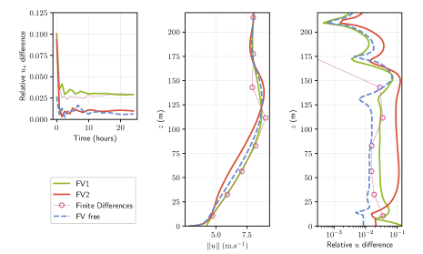
Figure 3: Relative difference between low-resolution and high-resolution simulations with several strategies for the SL handling. Left: Relative difference in $u_{\star}$ as a function of time. Center: vertical profiles of the wind speed at the end of the simulation. Right: Relative difference of the wind speed between low- and high-resolution along the vertical (note the log scale).

In the neutral case (constant density), the difference between low and high resolution of the “FV free” scheme is small at low altitude (see Fig. 3). This is mainly due to two factors:

• $\delta_{\rm a}=z_{\frac{1}{2}}^{\rm low-res}$ is the same for both low and high resolutions, whereas for the other surface flux schemes the continuous equations change with $\delta_{\rm a}$.

• The initial relative difference for $u_{\star}$ (Fig. 3, left panel) is already much smaller than with the other schemes. This is a consequence of the imposed wall law: at initialization, there is already a logarithmic profile in the surface layer, instead of evolving toward a kind of compromise between the parameterized and the modeled values.

Stratified case: We now focus on a stratified model [3] that includes more of the physical behavior of atmospheric models: the turbulence closure depends on the density $\rho$ such that $\partial_{z}\rho\propto-\partial_{z}\theta$ where $\theta$ is the potential temperature. We designed two cases:

1. A stable stratification, obtained with an initial temperature increasing with the altitude, and a surface temperature decreasing with time. The initial potential temperature is 265 K in the first 100 meters of the atmosphere and then gains 1 degree every 100 meters; the surface temperature starts at 265 K and loses 1 degree every ten hours. The “low resolution” uses 15 grid points in the 400m column and the “high resolution” uses 45 grid points.

2. An unstable stratification, obtained with a surface temperature following a daily oscillation between $279$ K and $281$ K, and initial profiles of temperature and wind set to constant values of $280$ K and $8\;{\rm m}.{\rm s}^{-1}$ respectively. The “low resolution” is composed of 50 grid levels of $10$m each; 15 additional stretched levels between $500$m and $1080$m make sure that the upper boundary condition is not involved in the results. The “high resolution” divides every space cell into 3 new space cells of equal sizes.

The differences between the two simulations are displayed in Fig. 4. In the stable case, the difference between the high resolution and the low resolution results does not significantly change with the surface flux schemes. The “FV2” scheme is not very consistent because it tries to follow the continuous model but with $\delta_{\rm a}$ changing with the resolution. The Finite Difference or the “FV1” methods suffer less from this problem because, even if $\delta_{\rm a}$ changes, it is assumed that the evolution equation is integrated inside the surface layer. In [9], authors also find that the sensitivity of their Large Eddy Simulation model to the grid spacing is “more likely related to under-resolved near-surface gradients and turbulent mixing at the boundary-layer top, to the [sub-grid scale] model formulation, and/or to numerical issues, and not to deficiencies due to the use of improper surface boundary conditions”.

In the unstable case, the “FV free” scheme (with $\delta_{\rm a}=z_{\frac{1}{2}}^{\rm low-res}$) seems much more robust than the other schemes in the first $200$ meters (remind that the height of the SL is approximately 10m). Above this height the differences between the high resolution and the low resolution simulations are not clearly influenced by the SL treatment. Note also that, as in the stable case, the “FV2” scheme is also less consistent: enforcing the MO theory in the first cell increases the sensitivity of the solution to $\delta_{\rm a}$ because the SL is then tightly coupled with the computational domain. Finally, the “FV free” scheme combines good consistency properties with a SL scheme coherent with the physical theory.

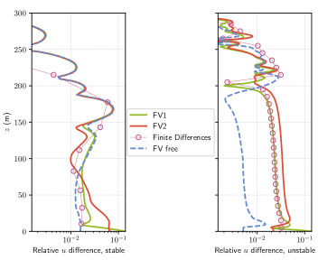
Figure 4: Relative difference of the wind speed between low- and high-resolution simulations for several SL strategies. left: stable stratification. Right: unstable stratification.

References

- [1] Clement, S.: Numerical analysis for a combined space-time discretization of air-sea exchanges and their parameterizations. PhD thesis, Université Grenoble Alpes (2022), ⟨tel-04066324⟩
- [2] Jaegle, F., Cabrit, O., Mendez, S., Poinsot, T.: Implementation methods of wall functions in cell-vertex numerical solvers. Flow Turbul Combust, 85, 245-272 (2010). doi:10.1007/s10494-010-9276-1
- [3] McWilliams, J. C., Huckle, E., and Shchepetkin, A. F.: Buoyancy Effects in a Stratified Ekman Layer. J. Phys. Oceanogr., 39, 2581–2599 (2009). doi:10.1175/2009JPO4130.1
- [4] Larsson, J., Kawai, S., Bodart, J., Bermejo-Moreno, I.: Large eddy simulation with modeled wall-stress : Recent progress and future directions. Mech. Eng. Rev., 3 (2016). doi:10.1299/mer.15-00418
- [5] Nishizawa, S., Kitamura, Y.: A Surface Flux Scheme Based on the Monin-Obukhov Similarity for Finite Volume Models. J. Adv. Model. Earth Syst., 12, 3159-3175 (2018). doi:10.1029/2018MS001534
- [6] Basu, S., Lacser, A.: A cautionary note on the use of Monin-Obukhov similarity theory in very high-resolution Large-Eddy Simulations. Bound.-Layer Meteorol., 163, pp. 351-355 (2017). doi:10.1007/s10546-016-0225-y
- [7] Piller, M. and Stalio, E.: Finite-volume compact schemes on staggered grids. Journal of Computational Physics, 197(1):299–340 (2004). doi:10.1016/j.jcp.2003.10.037
- [8] Clement, S.: Code for PhD thesis. Zenodo (2022). doi:10.5281/zenodo.7092357
- [9] Maronga, B., Knigge, C., Raasch, S.: An improved surface boundary condition for large-eddy simulations based on Monin–Obukhov similarity theory: evaluation and consequences for grid convergence in neutral and stable conditions. Bound.-Layer Meteorol., 174(2), 297-325 (2020). doi:10.1007/s10546-019-00485-w