Online Continual Learning Without the Storage Constraint

Abstract

Traditional online continual learning (OCL) research has primarily focused on mitigating catastrophic forgetting with fixed and limited storage allocation throughout an agent’s lifetime. However, a broad range of real-world applications are primarily constrained by computational costs rather than storage limitations. In this paper, we target such applications, investigating the online continual learning problem under relaxed storage constraints and limited computational budgets. We contribute a simple algorithm, which updates a kNN classifier continually along with a fixed, pretrained feature extractor. We selected this algorithm due to its exceptional suitability for online continual learning. It can adapt to rapidly changing streams, has zero stability gap, operates within tiny computational budgets, has low storage requirements by only storing features, and has a consistency property: It never forgets previously seen data. These attributes yield significant improvements, allowing our proposed algorithm to outperform existing methods by over 20% in accuracy on two large-scale OCL datasets: Continual LOCalization (CLOC) with 39M images and 712 classes and Continual Google Landmarks V2 (CGLM) with 580K images and 10,788 classes, even when existing methods retain all previously seen images. Furthermore, we achieve this superior performance with considerably reduced computational and storage expenses. We provide code to reproduce our results at https://github.com/drimpossible/ACM.

1 Introduction

Online continual learning algorithms need to update a model continuously over a stream of data originating from a non-stationary distribution. This requires them to solve a number of problems: they needs to successfully learn the main task (accuracy), adapt to changes in the distribution (rapid adaptation), and retain information from the past (prevent catastrophic forgetting). A key motif in recent work on online continual learning is the designing algorithms that achieve a good trade-off between these possibly competing objectives under resource constraints (Cai et al., 2021).

To establish the resource constraints for typical commercial settings, we first ask: what is required of continual learning algorithms? A continual learning algorithm must deliver accurate predictions, scale to large datasets encountered during its operational lifetime, and operate within the system’s total cost budget (in dollars). The economics of data storage have been studied since 1987 (Gray & Putzolu, 1987; Gray & Graefe, 1997; Graefe, 2009; Appuswamy et al., 2017). Table 1 summarizes the trends, show a rapid decline in storage costs over time ($\sim\$100$ to store CLOC, the largest dataset for OCL (Cai et al., 2021), in 2017). In contrast, training an ER baseline (Cai et al., 2021), the state-of-the-art OCL method on CLOC currently costs over $2000 on a GCP server and is still not commercially feasible on mobile devices. Consequently, computational constraints are the primary concern, with storage costs being relatively insignificant. Therefore, as long as computational costs are controlled, economically storing the entire incoming data stream is feasible.

However, online continual learning has primarily been studied under limited storage constraints (Lopez-Paz & Ranzato, 2017; Chaudhry et al., 2019a; Aljundi et al., 2019b), with learners only allowed to store a subset of incoming data. This constraint has led to many algorithms focusing on identifying a representative data subset (Aljundi et al., 2019b; Yoon et al., 2022; Chrysakis & Moens, 2020; Bang et al., 2021; Sun et al., 2022; Koh et al., 2022). While limited storage aligns with the practical constraints of biological learning agents and offline embodied artificial agents, deep learning-based systems are largely compute-constrained and demand high throughput. Such systems need to process incoming data points faster than the rate of the incoming stream to effectively keep up with the data stream. Cai et al. (2021) shows that even with unlimited storage, the online continual learning problem is hard as limited computational budgets implicitly limit the set of samples to be used for each training update. Our paper addresses the online continual learning problem, not from a storage limitation standpoint, but with a focus on computational budgets.

We propose a system based on approximate k-nearest neighbor (kNN) algorithm (Malkov & Yashunin, 2018) following its five desirable properties. i) Approximate kNNs are inherently incremental algorithms with explicit insert and retrieve operations allowing it to rapidly adapt to incoming data; ii) With a suitable representation, approximate kNN algorithms are exceptionally effective models at large-scale (Efros, 2017) iii) Approximate kNN algorithms are computationally cheap, with a graceful logarithmic scaling of computation despite compactly storing and using all past samples; iv) kNN does not forget past data. In other words, if a data point from history is queried again, the query yields the same label; v) It has no stability gap (De Lange et al., 2022) .

Table 1: The cost of storing data has decreased rapidly, allowing the storage of a large dataset for a negligible cost compared to the cost of computation for both cloud and mobile systems.

Cloud Storage	1987	1997	2007	2017
$/MB	83.33	0.22	0.0003	0.00002
Cost of storing CLOC ($)	350M	920K	1250	83
Training Cost (ER)	$>$2000$

Mobile NAND	2000	2005	2010	2017	2022
$/MB	1100	85	1.83	0.25	0.03
Cost of storing CLOC ($)	4M	300K	6350	850	70
Training Cost (ER)	Not Currently Feasible

Ideally, a continual learner should learn and update the feature representations over time. We defer this interesting problem to future work and instead show that combined with kNNs, it is possible for feature representations pre-trained on a relatively smaller dataset (Imagenet1K) to reasonably tackle complex tasks such as geolocalization over 39 million images (CLOC), and long-tailed fine-grained classification (CGLM). While this does not solve the underlying continual representation learning problem, it does show the effectiveness of a simple method on large-scale online continual learning problems, demonstrating viability to many real-world applications. Additionally, our approach overcomes a significant limitation of existing gradient-descent-based methods: the ability to learn from a single example. Updating a deep network for every incoming sample is computationally infeasible. In contrast, a kNN can efficiently learn from this sample, enabling rapid adaptation. We argue that the capacity to adapt to a single example while leveraging all past seen data is essential for truly online operation, allowing our simple method to outperform existing continual learning baselines.

Problem formulation. We formally define the online continual learning (OCL) problem following Cai et al. (2021). In classification settings, we aim to continually learn a function $f\colon\mathcal{X}\rightarrow\mathcal{Y}$, parameterized by $\theta_{t}$ at time $t$. OCL is an iterative process where each step consists of a learner receiving information and updating its model. Specifically, at each step $t$ of the interaction,

1. One data point $x_{t}\sim\pi_{t}$ sampled from a non-stationary distribution $\pi_{t}$ is revealed.

2. The learner makes the scalar prediction $\hat{y}_{t}=f(x_{t};\theta_{t})$ using a compute budget, $B^{pred}_{t}$.

3. Learner receives the true label $y_{t}$.

4. Learner updates the model $\theta_{t+1}$ using a compute budget, $B^{learn}_{t}$

We evaluate the performance using the metrics forward transfer (adaptability) and backward transfer (information retention) as given in Cai et al. (2021). A critical aspect of OCL is the budget in the second and fourth steps, which limits the computation that the learner can expend. A common choice in past work is to impose a fixed limit on storage and computation (Cai et al., 2021). We remove the storage constraint and argue that storing the entirety of the data is cost-effective as long as impact on computation is controlled. We relax the fixed computation constraint to a logarithmic constraint. In other words, we require that the computation time per operation fit within $B^{pred}_{t},B^{learn}_{t}\sim\mathcal{O}(\log t)$. This construction results in total cost scaling $\mathcal{O}(n\log n)$ with the amount of data.

2 Related Work

Table 2: Breakdown of popular OCL systems, with key contributions in red. Most methods focus on sampling techniques for storing datapoints, which cannot transfer here as we store all past samples.

Works	MemSamp	BatchSamp	Loss	Other Cont.
ER (Base)	Random	Random	CEnt	-
GSS (Aljundi et al., 2019b)	GSS	Random	CEnt	-
MIR (Aljundi et al., 2019a)	Reservoir	MIR	CEnt	-
ER-Ring (Chaudhry et al., 2019b)	RingBuf	Random	CEnt	-
GDumb (Prabhu et al., 2020)	GreedyBal	Random	CEnt	MR
HAL (Chaudhry et al., 2021)	RingBuf	Random	CEnt	HAL
CBRS (Chrysakis & Moens, 2020)	CBRS	Weighting	CEnt	-
CLIB (Koh et al., 2022)	ImpSamp	Random	CEnt	MR, AdO
CoPE (De Lange & Tuytelaars, 2021)	CBRS	Random	PPPLoss	-
CLOC (Cai et al., 2021)	FIFO	Random	CEnt	AdO
InfoRS (Sun et al., 2022)	InfoRS	Random	CEnt	-
OCS (Yoon et al., 2022)	OCS	Random	CEnt	-
AML (Caccia et al., 2022)	Reservoir	PosNeg	AML/ACE	-

Formulations. Parisi et al. (2019) and De Lange et al. (2020) have argued for improving the realism of online continual learning benchmarks. Earliest formulations (Lopez-Paz & Ranzato, 2017) worked in a task-incremental setup, assuming access to which subset of classes a test sample is from. Subsequent mainstream formulation (Aljundi et al., 2019b, a) required models to predict across all seen classes at test time, with progress in the train-time sample ordering (Bang et al., 2021; Koh et al., 2022). However, Prabhu et al. (2020) highlighted the limitations of current formulations by achieving good performance despite not using any unstored training data. Latest works (Hu et al., 2022; Cai et al., 2021; Lin et al., 2021) overcome this limitation by testing the capability for rapid adaptation to next incoming sample and eliminate data-ordering requirements by simply using timestamps of real-world data streams. Our work builds on the latest generation of formulation by Cai et al. (2021). Unlike Cai et al. (2021), we perform one-sample learning; in other words, we entirely remove the concept of task by processing the incoming stream one sample at a time, in a truly online manner. Additionally, we further remove the storage constraint which is the key to addressing issues discussed in GDumb (Prabhu et al., 2020).

Methods. Traditional methods of adapting to concept drift (Gama et al., 2014) include a variety of approaches based on SVMs (Laskov et al., 2006; Zheng et al., 2013), random forests (Gomes et al., 2017; Ristin et al., 2015; Mourtada et al., 2019), and other models (Oza & Russell, 2001; Mensink et al., 2013). They offer incremental additional and querying properties, most similar to our method, but have not been compared with recent continual learning approaches (Ostapenko et al., 2022; Hayes & Kanan, 2020; Hayes et al., 2019). We perform extensive comparisons with them.

The (online) continual learning methods designed for deep networks are typically based on experience replay (Chaudhry et al., 2019b) and change a subset of the three aspects summarized in Table 2: (i) the loss function used for learning, (ii) the algorithm to sample points into the replay buffer, and (iii) the algorithm to sample a batch from the replay buffer. Methods to sample points into the replay buffer include works such as GSS (Aljundi et al., 2019b), RingBuffer (Chaudhry et al., 2019b), class-balanced reservoir (Chrysakis & Moens, 2020), greedy balancing (Prabhu et al., 2020), rainbow memory (Bang et al., 2021), herding (Rebuffi et al., 2017), coreset selection (Yoon et al., 2022), information-theoretic reservoir (Sun et al., 2022), and samplewise importance (Koh et al., 2022). These approaches do not apply to our setting because we simply remove the storage constraint. Approaches to sampling batches from the replay buffer include MIR (Aljundi et al., 2019a), ASER (Shim et al., 2021), and AML (Caccia et al., 2022). These require mining hard negatives or performing additional updates for importance sampling over the stored data, which face scaling issues to large-scale storage as in our work. We compare with some of the above approaches, including ER as proposed in  Cai et al. (2021), that finetune the backbone deep network with one gradient update for incoming data, with unrestricted access to past samples for replay.

Pretrained representations. Pretrained representations (Yuan et al., 2021; Caron et al., 2021; Chen et al., 2021; Ali et al., 2021) have been utilized as initializations for continual learning, but in settings with harsh constraints on memory (Wu et al., 2022; Ostapenko et al., 2022). Inspired by Ostapenko et al. (2022), we additionally explore suitability of different pretrained representations. Another emerging direction for using pretrained models in continual learning has been prompt-tuning as it produces accurate classifiers while being computationally efficient (Wang et al., 2022b, a; Chen et al., 2023). However, Janson et al. (2022) show that simple NCM classification outperforms complex prompt tuning strategies. Lastly, the direction most similar to ours is methods which use kNN classifiers alongside deep networks for classification (Nakata et al., 2022; Iscen et al., 2022). We operate in significantly different setting and constraints, use far weaker pretrained representations (ImageNet1K) and benchmark on far larger online classification datasets.

3 Our Approach: Adaptive Continual Memory

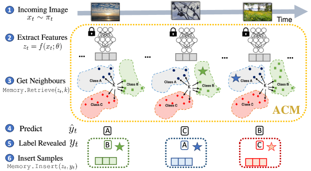
Figure 1: Adaptive Continual Memory (ACM) performs Memory.Retrieve and Memory.Insert on new incoming samples, extracted by a fixed, pretrained deep network.

We use pre-trained feature representations and only learn using the approximate k-nearest neighbor algorithm. Hence, our algorithm is rather simple. We refer to our algorithm as Adaptive Continual Memory (ACM) and refer to the kNN neighbour set as Memory. At each time step, our continual learner performs the following steps:

1. One data point $x_{t}\sim\pi_{t}$ sampled from a non-stationary distribution $\pi_{t}$ is revealed.

2. Learner extracts features $z_{t}=f(x_{t};\theta)$

3. Learner retrieves nearest neighbors $\mathcal{N}_{t}=\texttt{Memory.Retrieve}(z_{t},k)$.

4. Learner makes the prediction $\hat{y}_{t}=\texttt{majority-vote}(\mathcal{N}_{t})$.

5. Learner receives the true label $y_{t}$.

6. Learner inserts new data: $\texttt{Memory.Insert}(z_{t},y_{t})$.

We summarize this approach in Figure 1. Before presenting further implementation details, we discuss four properties of this method in detail.

Fast adaptation. Suppose the learner makes a mistake in a given time step. If the same data point is received in the next time step, the learner will produce the correct answer. By leveraging nearest neighbors, we enable the system to incorporate new data immediately and locally modify its answers in response to as little as a single datapoint. Such fast adaptation, a core desideratum in online continual learning, is infeasible with gradient descent strategies and is not presently a characteristic of deep continual learning systems.

Consistency. Consider a hypothetical scenario in which a data point is queried at multiple time instances. Our learner will never forget the correct label for this data point and will consistently produce it when queried, even after long time spans. While learning and memory are much more general than rote memorization, producing the correct answer on previously seen data is an informative sanity check. For comparison, continual learning on deep networks forgets a large fraction of previously seen datapoints even with a minimal delay (Toneva et al., 2019).

Zero Stability Gap. When learning new points, traditional continual learning algorithms first drop in performance on past samples due to a large drift from current minima and gradually recover performance on convergence. This phenomena is called as the stability gap (De Lange et al., 2022). Approximate kNN inherently does not have this optimization issue, hence enjoy zero stability gap.

Efficient Online Hyperparameter Optimization. Hyperparameter optimization is a critical issue during the online continual learning phase because, as distributions shifts, hyperparameters must be recalibrated. Selecting hyperparameters relevant to optimization like learning rate and batch size, can be nuanced; an incorrect choice has the potential to indefinitely impede future performance. Common strategies include executing multiple simultaneous online learning tasks using diverse parameters (Cai et al., 2021). However, this can be prohibitively resource-intensive. In contrast, our method has a single hyperparameter ($k$), which only affects the immediate prediction, and can be recalibrated during the online continual learning phase with minimal computational cost. We do this by first retrieving the $512$ nearest neighbours in a sorted order and subequently searching over smaller $k$ in powers of two within this ranked list, and selecting the $k$ which achieves highest accuracy on simulating arrival of previous samples.

3.1 Computational Cost and Storage Considerations

In the presented algorithm above for our method, feature extraction (step 2) and prediction (step 4) have a fixed overhead cost. However, nearest-neighbour retrieval (step 3) and inserting new data (step 6) can have high computational costs if done naively. However, literature in approximate k-nearest neighbours (Shakhnarovich et al., 2006) has shown that we can achieve high performance while significantly reducing computational complexity from linear $\mathcal{O}(n)$ to logarithmic $\mathcal{O}(\log n)$, where $n$ is the number of data points in memory. By switching from exact kNN to HNSW-kNN, we reduce the comparisons from 30 million to a few hundred, while maintaining a similar accuracy. We utilize the HNSW algorithm from HNSWlib because of its high accuracy, approximate guarantees and practically fast runtime on ANN Benchmarks (Aumüller et al., 2020). We use NMSLib (Malkov & Yashunin, 2018) with ef=500 and m=100 as default construction parameters. We perform a wall-clock time analysis quantifying this speed in Section 4.3.

4 Experiments

We first describe our experimental setup below and then provide comprehensive comparisons of our method against existing incremental learning approaches.

Datasets. We used a subset of Google Landmarks V2 and YFCC-100M datasets for online image classification. These datasets are ordered by the timestamps of image uploads, and our task is to predict the label of incoming images. We followed the online continual learning (OCL) protocol as described in Chaudhry et al. (2019a): We first tune hyperparameters of all OCL algorithms on a pretraining set, continually train the methods on the online training set while measuring rapid adaptation performance, and finally evaluated information retention on a unseen test set. Further dataset details are available in the Appendix.

Metrics. We follow Cai et al. (2021), measuring average online accuracy until the current timestep $t$ ($a_{t}$) as a metric for measuring rapid adaptation, given by $a_{t}=\nicefrac{{1}}{{t}}\sum_{i=1}^{t}\mathds{1}_{y_{i}=\hat{y}_{i}}$ where $\mathds{1}_{(\cdot)}$ is the indicator function. We additionally measure information retention, i.e. mitigating catastrophic forgetting, after online training on unseen samples from a test set. Formally, information retention for $h$ timesteps (${IR}_{h}$) at time $T$, is defined as ${IR}_{h}=\nicefrac{{1}}{{h}}\sum_{t=T-h}^{T}\mathds{1}_{y_{t}=\hat{y}_{t}}$.

Computational Budget and Pretraining. To ensure fairness among compared methods, we restrict the computational budget for all methods to one gradient update using the naive ER method. All methods were allowed to access all past samples with no storage restrictions. All methods started with a pretrained ResNet50 model on the ImageNet1K dataset for fairness. Note that we select the ImageNet1K pretrained ResNet50 because despite being a good initialization, is not sufficient by itself to perform well on the selected continual learning benchmarks. We select a fine grained landmark recognition benchmark over 10788 categories (CGLM), and a harder geolocalization task over a far larger dataset of 39 million samples (CLOC).

OCL Approaches. We compared five popular OCL approaches as described in (Ghunaim et al., 2023) on the CLOC dataset. For CGLM, we compare among the top two performing methods from CLOC. We provide a brief summary of the approaches:

1. ER (Cai et al., 2021): We use vanilla ER without PoLRS and ADRep (Cai et al., 2021) as they did not improve performance.

2. MIR (Aljundi et al., 2019a): It additionally uses MIR as the selection mechanism for choosing samples for training (in a task-free manner).

3. ACE (Caccia et al., 2022): ACE loss is used instead of cross entropy to reduce class interference.

4. LwF (Li & Hoiem, 2017): It adds a distillation loss to promote information retention.

5. RWalk (Chaudhry et al., 2018): This method adds a regularization term based on Fisher information matrix and optimization-path based importance scores. We treat each incoming batch of samples as a new task.

Training Details for Baselines. CGLM has the same optimal hyperparameters for CLOC. The ResNet50 model was continually updated using the hyperparameters outlined in (Ghunaim et al., 2023). We used a batch size of 64 for CGLM and 128 for CLOC to control the computational costs. Predictions are made on the next batch of 64/128 samples for CGLM/CLOC dataset respectively using the latest model. The model uses a batch size of 128/256 respectively for training, with the remaining batch used for replaying samples from storage.

Fixed Feature Extractor based Approaches. In this section, we ablate capabilities specifically contributed by kNN in ACM compared to other continual learning methods which use a common fixed feature extractor. However, the compared baselines do not have the consistency property provided by ACM, ablating the contribution of this property. We use a 2 layer embedder MLP to project the 2048 dimensional features of ResNet to 256 dimensions using the pretrain set. This adapts the pretrained features to domain of the tested dataset, while providing compact storage and increasing processing speed. All below methods operate on these fixed 256 dimensional features for fairness and operate on features normalized by an online scaler for best performance, with one sample incoming at a timestep. Note that the full model continual learning methods did not benefit significantly by this additional adaptation step. We detail the approaches below:

1. Nearest Class Mean (NCM) (Mensink et al., 2013; Rebuffi et al., 2017; Janson et al., 2022): This method maintains a mean feature for each class and classifies new samples by measuring cosine similarity with the mean feature.

2. Streaming LDA (SLDA) (Hayes et al., 2019): This is the current state-of-the-art online continual method using fixed-feature extractors. We use the code provided by the authors with $1e-4$ being optimal shrinkage parameter.

3. Incremental Logistic Classification (Tsai et al., 2014): We include traditional incremental logistic classification. We use scikit-learn SGDClassifier with Logistic loss.

4. Incremental SVM (Laskov et al., 2006): We include traditional online support vector classification. We use scikit-learn SGDClassifier with Hinge loss.

5. Adaptive Random Forests (ARF) (Gomes et al., 2017): We chose the best performing method from benchmarks provided by the River library called Adaptive Random Forests.

6. Eigen Memory Trees (EMT) (Rucker et al., 2022): This is the current state-of-the-art incremental learning method using Trees, outperforming Sun et al. (2019) by large margins.

4.1 Comparison of ACM with Online Continual learning Approaches

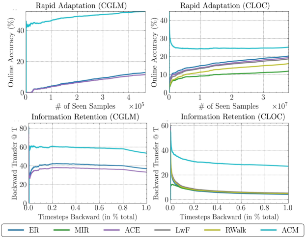
Figure 2: Online Continual Learning Performance. We observe that ACM outperforms existing methods by a large margin despite being far cheaper computationally. Traditional methods perform poorly given unrestricted access to past seen data indicating continual learning is a hard problem even without storage constraints.

Online adaptation. We compare the average online accuracy of ACM to state-of-the-art approaches on CGLM and CLOC datasets in Figure 2. We observe that ACM significantly outperforms previous methods, achieving a 35% and 5% higher absolute accuracy margin on CGLM and CLOC, respectively. This improvement is due to the capability of ACM to rapidly learn new information.

Information retention. We compare backward transfer of ACM to current state-of-the-art approaches on CGLM and CLOC in Figure 2. We find that ACM preserves past information much better than existing approaches, achieving 20% higher accuracy on both datasets. On the larger CLOC dataset, we discover that existing methods catastrophically forget nearly all past knowledge, while ACM maintains a fairly high cumulative accuracy across past timesteps. This highlights the advantages of the consistency property, allowing perfect recall of past train samples and subsequently, good generalization ability on similar unseen test samples to past data.

Moreover, comparing the performance of methods to those in the fast stream from Ghunaim et al. (2023), it becomes evident that removing memory restrictions (from 40,000 samples) did not substantially alter the performance of traditional OCL methods. This emphasizes that online continual learning with limited computation remains challenging even without storage constraints.

Key Takeaways. ACM demonstrates significantly better performance in both rapid adaptation and information retention when compared to popular continual learning algorithms which can update the base deep network on any of the past seen samples with no restrictions. We additionally highlight that ACM has a substantially lesser computational cost compared to traditional OCL methods.

4.2 Comparison of ACM with Approaches Leveraging a Fixed Backbone

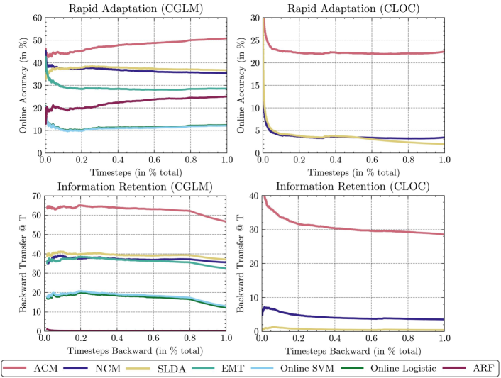
Figure 3: Online Continual Learning Performance. ACM outperforms existing methods which leverage a fixed backbone. This highlights the importance of preserving the consistency property in online continual learning. The collapse of other approaches for the CLOC dataset indicates the hardness of the continual learning scenario.

Online adaptation. We compare average online accuracy of ACM against recent continual learning approaches that also employ a fixed feature extractor on CGLM and CLOC datasets in Figure 3. We find that ACM outperforms these alternative approaches by significant margins, achieving 10% and 20% higher absolute accuracy on CGLM and CLOC respectively. All approaches here can rapidly adapt to every incoming sample, achieving higher accuracy than traditional OCL approaches. However, ACM can additionally utilizing past seen samples when necessary. Notably, in CLOC, the best alternative approaches collapse to random performance, highlighting that pretrained feature representations are not sufficient, and the effectiveness of kNN despite its simplicity.

Information retention. We compare backward transfer of ACM compared to other fixed-feature based OCL approaches on CGLM and CLOC dataset in Figure 3. We observe that ACM outperforms other apporaches by 20% on both datasets, demonstrating its remarkable ability to preserve past knowledge over time. Even after 39 million online updates on the CLOC, ACM preserves information from the earliest samples. In contrast, existing fixed-feature online continual learning methods collapse to random performance.

Key Takeaways. The impressive performance of ACM is evident in both rapid adaptation and information retention even amongst latest approaches which similarly use a fixed feature extractor. This further demonstrates the impact of preserving consistency.

A Note on Time. ACM and NCM were the fastest approaches among the compared methods. All other approaches were considerably slower, with a 5 to 100 fold increase in runtime compared with NCM or ACM. However, this could be attributed to codebases, although we used open-source, fast libraries such as River and Scikit-learn.

4.3 Analyzing Our Method: Adaptive Continual Memory

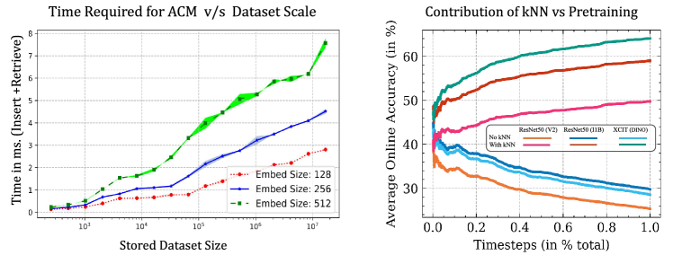
Figure 4: Left: Wall clock time overhead of using ACM Memory after feature extraction (x-axis is log-scaled) on a 16-core i7 CPU server. The time increases logarithmically with dataset size, with a 8ms overhead at 40M samples. Right: Contribution of kNN and contribution of the original backbone along with the MLP. We observe most of the performance is attributable to the kNN.

Contribution of kNN. Here, we aim to disentangle the benefit provided by the pretrained backbone and the domain tuning by the MLP, with the contribution of kNN to ACM. To test this, we perform online continual learning by replacing the kNN with the fixed MLP classifier. The performance obtained on rapid adaptation on ablating the kNN will be the effect of strong backbone and first session tuning using MLP on pretrain set (Panos et al., 2023). We conducted this experiment using two additional pretrained backbones stronger than our ResNet50 trained on ImageNet1K: A ResNet50 trained on Instagram 1B dataset and the best DINO model XCIT-DINO trained on Imagenet1K to vary the pretraining dataset and architecture.

The results presented in Figure 4 (right). We observe that removing the kNN for classification leads to a drastic decline in performance, indicating that kNN is the primary driver of performance, with performance gains of 20-30%. The decline in performance, losing over 10%, compared to initialization is attributable to distribution shift across time. This is consistently seen across model architectures, indicating that CGLM remains a challenging task with a fixed feature extractor despite backbones far stronger than ResNet50 trained on ImageNet1K.

These findings suggest that kNN is the primary reason for rapid adaptation gains to distribution shifts. Having high-quality feature representations alone or fist-session adaptation is insufficient for a satisfactory online continual learning performance.

Time Overhead of ACM. We provide a practical analysis of time to ground the logarithmic computational complexity of ACM. Figure 4 (left) provides insights into the wall-clock time required for the overhead cost imposed by ACM when scaling to datasets of 40 million samples. We observe that the computational overhead while using ACM scales logarithmically, reaching a maximum of approximately 5 milliseconds for 256 dimensional embeddings. In comparison, the time required for the classification of a single sample for deep models like ResNet50 is approximately 10 milliseconds on an Intel 16-core CPU. It’s important to note that when using ACM, the total inference cost of ACM inference would be 15 milliseconds, representing a 50% inference overhead as a tradeoff for high rapid adaptation and information retention performance.

4.4 Discussion

A notable limitation of our approach is its dependency on the presence of pretrained features. Consequently, our method may not be appropriate for situations where such features are unavailable. While this limitation is important to acknowledge, it doesn’t diminish the relevance of our approach in situations where pretrained features are available. Our method can be applied effectively in a wide range of visual continual learning scenarios. We have been selective in our choice of models and experiments, opting for pretrained models on ImageNet1K rather than larger models like CLIP or DINOv2 to demonstrate this applicability. Moreover, we tested our approach on more complex datasets like Continual YFCC-100M, which is 39 times larger than ImageNet1K and includes significantly more challenging geolocation tasks.

Memory constraints are often linked to privacy concerns. However, it’s crucial to understand that merely avoiding data storage does not guarantee privacy in continual learning. Given the tendency of deep neural networks to memorize information, ensuring privacy becomes a much bigger challenge. While a privacy-preserving adaptation of our method is beyond this paper’s scope, one can employ differentially private feature extractors, as suggested by (Ma et al., 2022), to build privacy-conscious ACM models. We conjecture that as more advanced privacy-preserving feature extractors become available, privacy concerns can be addressed in parallel.

Finally, to contextualize the computational budget with tangible figures, we envision a hypothetical system necessitating real-time operation on a video stream, facilitated by a 16-core i7 CPU server. Given a feature size of 256 and drawing insights from Figure 4, our method is projected to sustain real-time processing at 30 frames per second for an impressive span of up to 71 years, without necessitating further optimization. Such a configuration would consume approximately 900 GB of storage annually, translating to a cost of roughly $20 per year, as indicated in Table 1. Thus, the ACM stands out as practical, even for the prolonged deployment of continual learning systems.

5 Conclusion

In this work, we explored online continual learning without any storage constraints. Our reformulation emerges from an analysis of both economic and computational attributes of computing systems. We introduce an approximate kNN-based approach that stores the entirety of the data, adapts on a per-sample basis at each timestep, and still retains computational efficiency. Upon evaluation on large-scale OCL benchmarks, our system yields significant improvements over existing methods. Our approach is computationally cheap and scales gracefully to large-scale datasets.

6 Acknowledgements

This work is supportedin part by a UKRI grant: Turing AI Fellowship EP/W002981/1 and an EPSRC/MURI grant: EP/N019474/1. We would also like to thank the Royal Academy of Engineering and FiveAI. Ameya produced this work as part of his internship at Intel Labs. A special thanks to Hasan Abed Al Kader Hammoud for their help.

Appendix A Implementation Details

In this section, we describe the experimental setup in detail including dataset creation, methods and their training details.

A.1 Dataset Details

Continual Google Landmarks V2 (CGLM) (Weyand et al., 2020): We introduce a new dataset which is a subset of Google Landmarks V2 dataset (Weyand et al., 2020) as our second benchmark. We use the train-clean subset, filtering it further based on the availability of upload timestamps on Flickr. We filter out the classes that have less than 25 samples. We uniformly in random sample 10% of data for testing and then use the first 20% of the remaining data as a hyperparameter tuning set, similar to CLOC. We get $430K$ images for continual learning with $10788$ classes.

We start with the train-clean subset of the GLDv2 available from the dataset website. We apply the following preprocessing steps in order:

1. Filter out images which do not have timestamp metadata available.

2. Remove images of classes that have less than 25 samples in total

3. Order data by timestamp

We get the rest $580K$ images for continual learning over $10788$ classes with large class-imbalance alongside the rapid distribution shift temporally. We allocate the first 20% of the dataset timestampwise for pretraining and randomly sample 10% of data from across time for testing. We provide the scripts for cleaning the dataset alongside in the codebase.

Continual YFCC-100M (CYFCC) (Thomee et al., 2016): The subset of YFCC100M, which has date and time annotations (Cai et al., 2021). We follow their dataset splits. We order the images by timestep and iterate over 39 million online timesteps, one image at a time, with evaluation on the next image in the stream. Note that in contrast, Cai et al. (2021) uses a more restricted protocol assuming 256 images per timestep and evaluates on images uploaded by a different user in the next batch of samples. We download the images and the metadata as given by Cai et al. (2021) from their github repository. We provide a guide for downloading alongside in our codebase.

A.2 Model and Optimization Details

Training OCL approaches: We use a ResNet50-V2 model from Pytorch for all other methods. We trained models starting from a pretrained ImageNet1K model with a batch size of 128 for CGLM and 256 for CLOC with a constant lr of 5e-3, SGD optimizer as specified in the original work. We used a 80GB A100 GPU server for the training.

MLP Details: We use a 2-layer MLP consisting of (input, embedding) and (embedding, output) layers, with batchnorm and ReLU activations trained for 10 epochs on CGLM pretrain set and 2 epochs on the CLOC pretrain set. We do not do hyperparameter optimization and use the default parameters as hyperparameter optimization in online continual learning is an open problem. All ACM experiments were performed on one 48 GB RTX 6000 to extract features and the kNN computation was done on a 12th Gen Intel i7-12700 server.

Appendix B Evaluating Rapid Adaptation Using Near-Future Accuracy

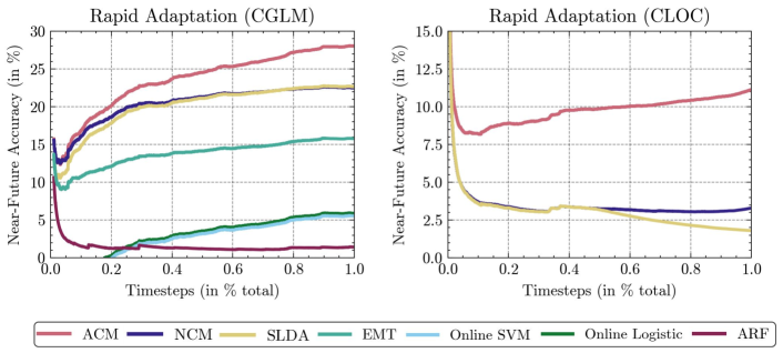
Figure 5: Online Continual Learning Performance. We observe that ACM outperforms existing methods on the near-future accuracy metric by 5-10%, maintaining state-of-the-art performance.

Evaluation of Rapid Adaptation using Near-Future Accuracy. Hammoud et al. (2023) discovered label correlations in the original online accuracy metric used for evaluating online continual learning methods. However, ACM remained state-of-the-art performance on their fast stream setting, despite performance of other methods falling below offline learning baselines.

In this section, we compare the performance of ACM to other online learning approaches with a fixed feature extractor on CGLM and CLOC datasets with the near-future accuracy metric using the same delay parameters (Hammoud et al., 2023). We present our results in Figure 5. We observe that ACM achieves state-of-the-art performance among online continual learning approaches, outperforming them by 5-10% margins. This provides us with additional evidence to indicate that ACM did not exploit on label correlations to achieve high online accuracy.

Appendix C Additional Experiments

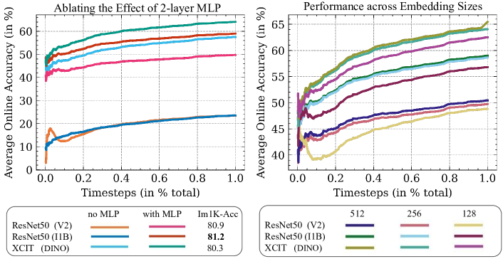
Figure 6: Left: Ablating the effect of first-session adaptation using an MLP. We observed first-session adaptation caused minor improvement in performance on XCIT model with 512 dimensional features, however provided a major performance boost for 2048 dimensional ResNet50 features. Right: Ablating the effect of embedding dimensions. We observe that varying the embedding size allows a tradeoff between computational cost and accuracy. However, it does not cause dramatic increase or decrease in performance.

Ablating the contribution of the 2-layer MLP. We ablate the contribution of first-session adaptation (Panos et al., 2023) on the pretraining set. We compare online learning performance with and without using the MLP and present the results across different models in Figure 6 (left). We observe that the performance in XCIT DINO model achieves a performance boost of 5% when using the MLP, indicating that first-session adaptation allows for an improvement in performance. However, both ResNet50 models gain large improvements of over 30% in online accuracy due to the MLP. We notice that this is attributable to the curse of dimensionality. ResNet50 architecture has a far larger feature dimension of 2048 in compared to XCIT-DINO having 512 dimensions. Comparing models with MLP, we surprisingly observe that ResNet50-I1B performs worse than XCIT-DINO model despite ResNet50-I1B achieving better performance across traditional benchmarks, indicative of robust and generalizable features. We conclude that ResNet50 architecture is a poor fit for ACM due to 2048 dimensional features.

Conclusion. Models with high-dimensional embeddings perform much more poorly in combination with a kNN despite better representational power due to the curse of dimensionality.

Ablating the effect of the embedding size. We now know that embedding dimensions can significantly affect performance. We vary the embedding dimensions to explore the sensitivity of ACM to embedding dimensions. We start with 512 dimensional XCIT feature dimensions, varying the embedding sizes to 512, 256 and 128.

We present the results in Figure 6 (right). First, we observe that decreasing the embedding dimension to 256 results in minimal drop in accuracy across all the three models but reduces the computational costs by half as shown in Figure 4 in the main paper. Further reduction in embedding dimension leads to considerable loss of performance. An embedding size of 256 achieves the best tradeoff between speed and accuracy.

References

- Ali et al. (2021) Alaaeldin Ali, Hugo Touvron, Mathilde Caron, Piotr Bojanowski, Matthijs Douze, Armand Joulin, Ivan Laptev, Natalia Neverova, Gabriel Synnaeve, Jakob Verbeek, et al. Xcit: Cross-covariance image transformers. NeurIPS, 2021.
- Aljundi et al. (2019a) Rahaf Aljundi, Lucas Caccia, Eugene Belilovsky, Massimo Caccia, Laurent Charlin, and Tinne Tuytelaars. Online continual learning with maximally interfered retrieval. In NeurIPS, 2019a.
- Aljundi et al. (2019b) Rahaf Aljundi, Min Lin, Baptiste Goujaud, and Yoshua Bengio. Gradient based sample selection for online continual learning. In NeurIPS, 2019b.
- Appuswamy et al. (2017) Raja Appuswamy, Renata Borovica-Gajic, Goetz Graefe, and Anastasia Ailamaki. The five-minute rule thirty years later and its impact on the storage hierarchy. In ADMS@VLDB, 2017.
- Aumüller et al. (2020) Martin Aumüller, Erik Bernhardsson, and Alexander John Faithfull. Ann-benchmarks: A benchmarking tool for approximate nearest neighbor algorithms. Inf. Syst., 87, 2020.
- Bang et al. (2021) Jihwan Bang, Heesu Kim, YoungJoon Yoo, Jung-Woo Ha, and Jonghyun Choi. Rainbow memory: Continual learning with a memory of diverse samples. In CVPR, 2021.
- Caccia et al. (2022) Lucas Caccia, Rahaf Aljundi, Nader Asadi, Tinne Tuytelaars, Joelle Pineau, and Eugene Belilovsky. New insights on reducing abrupt representation change in online continual learning. ICLR, 2022.
- Cai et al. (2021) Zhipeng Cai, Ozan Sener, and Vladlen Koltun. Online continual learning with natural distribution shifts: An empirical study with visual data. In ICCV, 2021.
- Caron et al. (2021) Mathilde Caron, Hugo Touvron, Ishan Misra, Hervé Jégou, Julien Mairal, Piotr Bojanowski, and Armand Joulin. Emerging properties in self-supervised vision transformers. In ICCV, 2021.
- Chaudhry et al. (2018) Arslan Chaudhry, Puneet K Dokania, Thalaiyasingam Ajanthan, and Philip HS Torr. Riemannian walk for incremental learning: Understanding forgetting and intransigence. In Proceedings of the European conference on computer vision (ECCV), pp. 532–547, 2018.
- Chaudhry et al. (2019a) Arslan Chaudhry, Marc’Aurelio Ranzato, Marcus Rohrbach, and Mohamed Elhoseiny. Efficient lifelong learning with a-gem. In ICLR, 2019a.
- Chaudhry et al. (2019b) Arslan Chaudhry, Marcus Rohrbach, Mohamed Elhoseiny, Thalaiyasingam Ajanthan, Puneet K Dokania, Philip HS Torr, and Marc’Aurelio Ranzato. Continual learning with tiny episodic memories. In ICML-W, 2019b.
- Chaudhry et al. (2021) Arslan Chaudhry, Albert Gordo, David Lopez-Paz, Puneet K. Dokania, and Philip Torr. Using hindsight to anchor past knowledge in continual learning, 2021.
- Chen et al. (2023) Haoran Chen, Zuxuan Wu, Xintong Han, Menglin Jia, and Yu-Gang Jiang. Promptfusion: Decoupling stability and plasticity for continual learning. arXiv preprint arXiv:2303.07223, 2023.
- Chen et al. (2021) Xinlei Chen, Saining Xie, and Kaiming He. An empirical study of training self-supervised vision transformers. In ICCV, 2021.
- Chrysakis & Moens (2020) Aristotelis Chrysakis and Marie-Francine Moens. Online continual learning from imbalanced data. In ICML, 2020.
- De Lange & Tuytelaars (2021) Matthias De Lange and Tinne Tuytelaars. Continual prototype evolution: Learning online from non-stationary data streams. In ICCV, 2021.
- De Lange et al. (2020) Matthias De Lange, Rahaf Aljundi, Marc Masana, Sarah Parisot, Xu Jia, Ales Leonardis, Gregory G. Slabaugh, and Tinne Tuytelaars. Continual learning: A comparative study on how to defy forgetting in classification tasks. In TPAMI, 2020.
- De Lange et al. (2022) Matthias De Lange, Gido van de Ven, and Tinne Tuytelaars. Continual evaluation for lifelong learning: Identifying the stability gap. arXiv preprint arXiv:2205.13452, 2022.
- Efros (2017) Alexei Efros. How to stop worrying and learn to love nearest neighbors. 2017. URL https://nn2017.mit.edu/wp-content/uploads/sites/5/2017/12/Efros-NIPS-NN-17.pdf.
- Gama et al. (2014) João Gama, Indrė Žliobaitė, Albert Bifet, Mykola Pechenizkiy, and Abdelhamid Bouchachia. A survey on concept drift adaptation. ACM computing surveys, 2014.
- Ghunaim et al. (2023) Yasir Ghunaim, Adel Bibi, Kumail Alhamoud, Motasem Alfarra, Hasan Abed Al Kader Hammoud, Ameya Prabhu, Philip HS Torr, and Bernard Ghanem. Real-time evaluation in online continual learning: A new paradigm. In IEEE/CVF Conference on Computer Vision and Pattern Recognition (CVPR), 2023.
- Gomes et al. (2017) Heitor M Gomes, Albert Bifet, Jesse Read, Jean Paul Barddal, Fabrício Enembreck, Bernhard Pfharinger, Geoff Holmes, and Talel Abdessalem. Adaptive random forests for evolving data stream classification. Machine Learning, 2017.
- Graefe (2009) Goetz Graefe. The five-minute rule 20 years later (and how flash memory changes the rules). Communications ACM, 2009.
- Gray & Graefe (1997) Jim Gray and Goetz Graefe. The five-minute rule ten years later, and other computer storage rules of thumb. ACM SIGMOD, 1997.
- Gray & Putzolu (1987) Jim Gray and Franco Putzolu. The 5 minute rule for trading memory for disc accesses and the 10 byte rule for trading memory for cpu time. In ACM SIGMOD, 1987.
- Hammoud et al. (2023) Hasan Abed Al Kader Hammoud, Ameya Prabhu, Ser-Nam Lim, Philip HS Torr, Adel Bibi, and Bernard Ghanem. Rapid adaptation in online continual learning: Are we evaluating it right? ICCV, 2023.
- Hayes & Kanan (2020) Tyler L Hayes and Christopher Kanan. Lifelong machine learning with deep streaming linear discriminant analysis. In CVPR-W, 2020.
- Hayes et al. (2019) Tyler L Hayes, Nathan D Cahill, and Christopher Kanan. Memory efficient experience replay for streaming learning. In ICRA, 2019.
- Hu et al. (2022) Hexiang Hu, Ozan Sener, Fei Sha, and Vladlen Koltun. Drinking from a firehose: Continual learning with web-scale natural language. IEEE Transactions on Pattern Analysis and Machine Intelligence, to appear, 2022.
- Iscen et al. (2022) Ahmet Iscen, Thomas Bird, Mathilde Caron, Alireza Fathi, and Cordelia Schmid. A memory transformer network for incremental learning. arXiv preprint arXiv:2210.04485, 2022.
- Janson et al. (2022) Paul Janson, Wenxuan Zhang, Rahaf Aljundi, and Mohamed Elhoseiny. A simple baseline that questions the use of pretrained-models in continual learning. arXiv preprint arXiv:2210.04428, 2022.
- Koh et al. (2022) Hyunseo Koh, Dahyun Kim, Jung-Woo Ha, and Jonghyun Choi. Online continual learning on class incremental blurry task configuration with anytime inference. ICLR, 2022.
- Laskov et al. (2006) Pavel Laskov, Christian Gehl, Stefan Krüger, Klaus-Robert Müller, Kristin P Bennett, and Emilio Parrado-Hernández. Incremental support vector learning: Analysis, implementation and applications. JMLR, 2006.
- Li & Hoiem (2017) Zhizhong Li and Derek Hoiem. Learning without forgetting. TPAMI, 2017.
- Lin et al. (2021) Zhiqiu Lin, Jia Shi, Deepak Pathak, and Deva Ramanan. The clear benchmark: Continual learning on real-world imagery. In NeurIPS, 2021.
- Lopez-Paz & Ranzato (2017) David Lopez-Paz and Marc’Aurelio Ranzato. Gradient episodic memory for continual learning. In NeurIPS, 2017.
- Ma et al. (2022) Yecheng Jason Ma, Shagun Sodhani, Dinesh Jayaraman, Osbert Bastani, Vikash Kumar, and Amy Zhang. Vip: Towards universal visual reward and representation via value-implicit pre-training. arXiv preprint arXiv:2210.00030, 2022.
- Malkov & Yashunin (2018) Yu A Malkov and Dmitry A Yashunin. Efficient and robust approximate nearest neighbor search using hierarchical navigable small world graphs. TPAMI, 2018.
- Mensink et al. (2013) Thomas Mensink, Jakob Verbeek, Florent Perronnin, and Gabriela Csurka. Distance-based image classification: Generalizing to new classes at near-zero cost. TPAMI, 2013.
- Mourtada et al. (2019) Jaouad Mourtada, Stéphane Gaïffas, and Erwan Scornet. Amf: Aggregated mondrian forests for online learning. Journal of the Royal Statistical Society, 2019.
- Nakata et al. (2022) Kengo Nakata, Youyang Ng, Daisuke Miyashita, Asuka Maki, Yu-Chieh Lin, and Jun Deguchi. Revisiting a knn-based image classification system with high-capacity storage. In European Conference on Computer Vision (ECCV), 2022.
- Ostapenko et al. (2022) Oleksiy Ostapenko, Timothee Lesort, Pau Rodríguez, Md Rifat Arefin, Arthur Douillard, Irina Rish, and Laurent Charlin. Continual learning with foundation models: An empirical study of latent replay. In Conference on Lifelong Learning Agents (CoLLAs), 2022.
- Oza & Russell (2001) Nikunj C Oza and Stuart J Russell. Online bagging and boosting. In International Workshop on Artificial Intelligence and Statistics. PMLR, 2001.
- Panos et al. (2023) Aristeidis Panos, Yuriko Kobe, Daniel Olmeda Reino, Rahaf Aljundi, and Richard E Turner. First session adaptation: A strong replay-free baseline for class-incremental learning. arXiv preprint arXiv:2303.13199, 2023.
- Parisi et al. (2019) German I Parisi, Ronald Kemker, Jose L Part, Christopher Kanan, and Stefan Wermter. Continual lifelong learning with neural networks: A review. Neural Networks, 2019.
- Prabhu et al. (2020) Ameya Prabhu, Philip HS Torr, and Puneet K Dokania. Gdumb: A simple approach that questions our progress in continual learning. In ECCV, 2020.
- Rebuffi et al. (2017) Sylvestre-Alvise Rebuffi, Alexander Kolesnikov, Georg Sperl, and Christoph H Lampert. icarl: Incremental classifier and representation learning. In CVPR, 2017.
- Ristin et al. (2015) Marko Ristin, Matthieu Guillaumin, Juergen Gall, and Luc Van Gool. Incremental learning of random forests for large-scale image classification. TPAMI, 2015.
- Rucker et al. (2022) Mark Rucker, Joran T Ash, John Langford, Paul Mineiro, and Ida Momennejad. Eigen memory tree. arXiv preprint arXiv:2210.14077, 2022.
- Shakhnarovich et al. (2006) Gregory Shakhnarovich, Trevor Darrell, and Piotr Indyk. Nearest-Neighbor Methods in Learning and Vision: Theory and Practice. The MIT Press, 2006.
- Shim et al. (2021) Dongsub Shim, Zheda Mai, Jihwan Jeong, Scott Sanner, Hyunwoo Kim, and Jongseong Jang. Online class-incremental continual learning with adversarial shapley value. In AAAI, 2021.
- Sun et al. (2022) Shengyang Sun, Daniele Calandriello, Huiyi Hu, Ang Li, and Michalis Titsias. Information-theoretic online memory selection for continual learning. ICLR, 2022.
- Sun et al. (2019) Wen Sun, Alina Beygelzimer, Hal Daumé Iii, John Langford, and Paul Mineiro. Contextual memory trees. In ICML, 2019.
- Thomee et al. (2016) Bart Thomee, David A Shamma, Gerald Friedland, Benjamin Elizalde, Karl Ni, Douglas Poland, Damian Borth, and Li-Jia Li. Yfcc100m: The new data in multimedia research. Communications of the ACM, 2016.
- Toneva et al. (2019) Mariya Toneva, Alessandro Sordoni, Remi Tachet des Combes, Adam Trischler, Yoshua Bengio, and Geoffrey J Gordon. An empirical study of example forgetting during deep neural network learning. In ICLR, 2019.
- Tsai et al. (2014) Cheng-Hao Tsai, Chieh-Yen Lin, and Chih-Jen Lin. Incremental and decremental training for linear classification. In KDD, 2014.
- Wang et al. (2022a) Zifeng Wang, Zizhao Zhang, Sayna Ebrahimi, Ruoxi Sun, Han Zhang, Chen-Yu Lee, Xiaoqi Ren, Guolong Su, Vincent Perot, Jennifer Dy, et al. Dualprompt: Complementary prompting for rehearsal-free continual learning. In European Conference on Computer Vision (ECCV), 2022a.
- Wang et al. (2022b) Zifeng Wang, Zizhao Zhang, Chen-Yu Lee, Han Zhang, Ruoxi Sun, Xiaoqi Ren, Guolong Su, Vincent Perot, Jennifer Dy, and Tomas Pfister. Learning to prompt for continual learning. In IEEE/CVF Conference on Computer Vision and Pattern Recognition (CVPR), 2022b.
- Weyand et al. (2020) T. Weyand, A. Araujo, B. Cao, and J. Sim. Google Landmarks Dataset v2 - A Large-Scale Benchmark for Instance-Level Recognition and Retrieval. In CVPR, 2020.
- Wu et al. (2022) Tz-Ying Wu, Gurumurthy Swaminathan, Zhizhong Li, Avinash Ravichandran, Nuno Vasconcelos, Rahul Bhotika, and Stefano Soatto. Class-incremental learning with strong pre-trained models. In IEEE/CVF Conference on Computer Vision and Pattern Recognition (CVPR), 2022.
- Yoon et al. (2022) Jaehong Yoon, Divyam Madaan, Eunho Yang, and Sung Ju Hwang. Online coreset selection for rehearsal-based continual learning. ICLR, 2022.
- Yuan et al. (2021) Lu Yuan, Dongdong Chen, Yi-Ling Chen, Noel Codella, Xiyang Dai, Jianfeng Gao, Houdong Hu, Xuedong Huang, Boxin Li, Chunyuan Li, et al. Florence: A new foundation model for computer vision. arXiv preprint arXiv:2111.11432, 2021.
- Zheng et al. (2013) Jun Zheng, Furao Shen, Hongjun Fan, and Jinxi Zhao. An online incremental learning support vector machine for large-scale data. Neural Computing and Applications, 2013.