Convex optimization over a probability simplex

James Chok
School of Mathematics and
Maxwell Institute for Mathematical Sciences,
The University of Edinburgh,
Edinburgh,
EH9 3FD,
United Kingdom
james.chok@ed.ac.uk
&Geoffrey M. Vasil
School of Mathematics and
Maxwell Institute for Mathematical Sciences,
The University of Edinburgh,
Edinburgh,
EH9 3FD,
United Kingdom
gvasil@ed.ac.uk
Abstract

We propose a new iteration scheme, the Cauchy-Simplex, to optimize convex problems over the probability simplex $\{w\in\mathbb{R}^{n}\ |\ \sum_{i}w_{i}=1\ \textrm{and}\ w_{i}\geq 0\}$. Other works have taken steps to enforce positivity or unit normalization automatically but never simultaneously within a unified setting. This paper presents a natural framework for manifestly requiring the probability condition. Specifically, we map the simplex to the positive quadrant of a unit sphere, envisage gradient descent in latent variables, and map the result back in a way that only depends on the simplex variable. Moreover, proving rigorous convergence results in this formulation leads inherently to tools from information theory (e.g. cross entropy and KL divergence). Each iteration of the Cauchy-Simplex consists of simple operations, making it well-suited for high-dimensional problems. We prove that it has a convergence rate of $\mathcal{O}(1/T)$ for convex functions, and numerical experiments of projection onto convex hulls show faster convergence than similar algorithms. Finally, we apply our algorithm to online learning problems and prove the convergence of the average regret for (1) Prediction with expert advice and (2) Universal Portfolios.

Keywords  Constrained Optimization, Convex Hull, Simplex, Universal Portfolio, Online Learning, Simplex Constrained Regression, Examinations, Convergence, Gradient Flow

MSCcodes  65K10, 68W27, 68W40, 91G10, 97U40

1 Introduction

Optimization over the probability simplex, (i.e., unit simplex) occurs in many subject areas, including portfolio management [1, 2, 3], machine learning [4, 5, 6, 7], population dynamics [8, 9], and multiple others including statistics and chemistry [10, 11, 12, 13]. This problem involves minimizing a function $f(w)$ (assumed convex) with $w\in\mathbb{R}^{n}$ within the probability simplex,

$\displaystyle\min_{w\in\Delta^{n}}f(w),\quad\textrm{where }\Delta^{n}=\{w\in\mathbb{R}^{n}\ |\ \sum_{i}w_{i}=1\ \textrm{and}\ w_{i}\geq 0\}.$ (1)

While linear and quadratic programs can produce an exact solution under certain restrictions on $f$, they tend to be computationally expensive when $n$ is large. Here we provide an overview of iterative algorithms to solve this problem approximately and introduce a new algorithm to solve this problem for general convex functions $f$.

Previous works each enforce one facet of the simplex constraint, positivity, or the unit-sum. Thus requiring an extra step to satisfy the remaining constraint. Our proposed method manages to satisfy both constraints, and we see the ideas encapsulated by these previous attempts within it.

2 Previous Works

Projected gradient descent (PGD) is a simple method to solve any convex problem over any domain $R$. The iteration scheme follows

$\displaystyle{w}^{t+1}=\textrm{proj}_{R}(w^{t}-\alpha_{t}\nabla f),$ (2)

where $\textrm{proj}_{R}$ is the projection of a point into $R$. Since the step $w^{t}-\alpha_{t}\nabla f$ does not preserve positivity, an explicit solution to the projection cannot be written. However, algorithms exist to perform projection into the unit simplex in $O(n)$ time111Assuming addition, subtraction, multiplication, and division take $\mathcal{O}(1)$ time. [14, 15], where $n$ is the dimension of $w$. While this added cost is typically negligible, once $n$ is big, it adds a high cost to each iteration.

This formulation of PGD can be simplified with linear constraints $Aw=b$, where $A$ is an $k\times n$ matrix and $b\in\mathbb{R}^{k}$. As suggested in [16, 17, 18, 19], a straightforward update scheme projects $\nabla f$ into the nullspace of $A$ and descends the result along the projected direction. For the unit-sum constraint, this algorithm requires solving the constrained optimization problem

$$\arg\min_{x}\frac{1}{2}\|\nabla f-x\|^{2},\quad\text{with}\quad\sum_{i}x_{i}=0.$$ (3)

This problem yields to the method of Lagrange multipliers, giving the solution

$$w^{t+1}=w^{t}-\alpha_{t}\left(\nabla f-\frac{1}{n}\sum_{i}\nabla_{i}f\right).$$ (4)

While this scheme satisfies the unit-sum constraint, in a similar manner to (2), it does not satisfy the positivity constraint. Thus requiring an additional projection with no explicit solution [20, 18].

Exponentiated Gradient Descent (EGD), first presented by Nemirovsky and Yudin [21] and later by Kivinen and Warmuth [22], instead enforces positivity by using exponentials, i.e.,

$\displaystyle w_{i}^{t+1}=\frac{w_{i}^{t}\exp(-\alpha_{t}\nabla_{i}f)}{\sum_{j}w_{j}^{t}\exp(-\alpha_{t}\nabla_{j}f)}.$ (5)

In the proper formulation of EGD, there is no normalizing factor, giving the iteration scheme $w^{t+1}=w^{t}\exp(-\alpha_{t}\nabla f)$. Thus preserving positivity but not the unit-sum constraint. However, preserving positivity yields an explicit solution for the projection onto the simplex, given by the normalizing factor. In this case, projection requires $\mathcal{O}(1)$ time.

Projection-free methods, instead, require each iteration to remain explicitly within the domain.

The Frank-Wolfe method is a classic scheme [23] that is experiencing a recent surge popularity [24, 25, 26, 27]. The method skips projection by assuming $R$ is convex. That is,

$\displaystyle w^{t+1}=(1-\gamma_{t})w^{t}+\gamma_{t}s^{t},$ (6)
$\displaystyle\textrm{where}\quad s^{t}=\arg\min_{s\in R}\ s\cdot\nabla f\quad\textrm{and}\quad 0\leq\gamma_{t}\leq 1.$

Since $R$ is convex, $w^{t+1}\in R$ automatically. Frank-Wolfe-based methods tend to be fast for sparse solutions but display oscillatory behavior near the solution, resulting in slow convergence [28, 29].

The Pairwise Frank-Wolfe (PFW) method improves upon the original by introducing an ‘away-step’ to prevent oscillations allowing faster convergence [30, 28, 31].

A well-studied [8, 32, 33, 34, 35, 36, 37] formulation of (1) takes $f$ to be quadratic, known as the standard quadratic optimization problem. In these situations, a line search has analytical solutions for the Frank-Wolfe and PFW methods but not for EGD and PGD. EGD and PGD require approximate methods (e.g. backtracking method [38]), adding extra run time per iteration.

3 The Main Algorithm

For convex problems over a probability simplex, we propose what we named the Cauchy-Simplex (CS)

$\displaystyle w^{t+1}=w^{t}-\eta_{t}d^{t},\quad$ (7)
$\displaystyle\text{with}\ d^{t}=w^{t}(\nabla f-w^{t}\cdot\nabla f),\quad\quad 0<\eta_{t}\leq{\eta}_{t,\max},$
$\displaystyle\text{and}\ \eta^{-1}_{t,\max}=\max_{i}(\nabla_{i}f-w^{t}\cdot\nabla f).$

The upper bound on the learning rate ${\eta}_{t}$ ensures that $w^{t+1}_{i}$ is positive for all $i$. Summing over the indices of $d^{t}$

$\displaystyle\sum_{i}w_{i}^{t}(\nabla_{i}f-w^{t}\cdot\nabla f)=(w^{t}\cdot\nabla f)\bigg{(}1-\sum_{i}w_{i}^{t}\bigg{)}.$ (8)

Thus, if $\sum_{i}w^{t}_{i}=1$ then $d^{t}$ lies in the null space of $\sum_{i}w_{i}$ and $w^{t+1}$ satisfies the unit-sum constraint. Hence giving a scheme where each iteration remains explicitly within the probability simplex, much like projection-free methods.

3.1 Motivating Derivation

Our derivation begins by modeling $w$ through a latent variable, $\psi$,

$\displaystyle w_{i}=\frac{\psi_{i}^{2}}{\sum_{j}\psi_{j}^{2}},$ (9)

which automatically satisfies positivity and unit probability. Now consider gradient descent on $\psi$,

$$\frac{d\psi}{dt}=-\alpha\frac{\partial f}{\partial\psi},\quad\textrm{with}\quad\alpha>0.$$ (10)

Using the notation $\dot{\psi}=d\psi/dt$, the chain rule gives

$\displaystyle\frac{dw}{dt}=\sum_{j}\frac{\partial w}{\partial\psi_{j}}\frac{d\psi_{j}}{dt}=\frac{2}{\|\psi\|^{2}}\bigg{(}\psi\,\dot{\psi}-w\,\psi\cdot\dot{\psi}\bigg{)}.$ (11)

Computing the derivatives and simplifying them gives

$$\frac{dw}{dt}=\frac{2}{\|\psi\|^{2}}\,\psi\,\dot{\psi}=-\beta w(\nabla f-w\cdot\nabla f)\quad\textrm{where}\quad\beta=\frac{4\alpha}{\|\psi\|^{2}},$$ (12)

where $\nabla f=\nabla_{w}f$. Thus giving the iterative scheme

$$w^{t+1}=w^{t}-\eta_{t}d^{t}\quad\text{where}\quad d^{t}=w^{t}(\nabla f-w^{t}\cdot\nabla f).$$ (13)

3.2 On the Learning Rate

Unlike EGD and PGD, but similar to Frank-Wolfe and PFW, each iteration of the CS has a maximum possible learning rate $\eta_{t,\max}$. This restriction may affect the numerical performance of the algorithm. To ease this problem, note that once an index is set to zero, it will remain zero and can be ignored. Giving an altered maximum learning rate

$\displaystyle\tilde{\eta}_{t,\max}=\frac{1}{\max_{i\in S}(\nabla_{i}f-w^{t}\cdot\nabla f)},$ (14)

where $S=\{i\ |\ w_{i}>0\}$. It follows that $\eta_{t,\max}\leq\tilde{\eta}_{t,\max}$, allowing for larger step-sizes to be taken.

3.3 Connections to Previous Methods

There are two other ways of writing the Cauchy-Simplex. In terms of the flow in $w$:

$$\frac{dw}{dt}=-W\Pi_{w}\nabla f,\quad\text{where}\quad\Pi_{w}=\textrm{I}-\mathbbm{1}\otimes w,$$ (15)

and $W$ is a diagonal matrix filled with $w$, I is the identity matrix, and $\mathbbm{1}$ is a vector full of 1s.

In terms of the flow in $\log(w)$:

$$\frac{d}{dt}\log(w)=-\Pi_{w}\nabla f,$$ (16)

giving an alternative exponential iteration scheme

$$w^{t+1}=w^{t}\exp(-\eta_{t}\Pi_{w}\nabla f).$$ (17)
Claim 1.

$\Pi_{w}$ is a projection provided $\sum_{i}w_{i}=1$.

Proof.

By direct computation,

$\displaystyle\Pi^{2}_{w}$ $\displaystyle=$ $\displaystyle\textrm{I}^{2}-2(\mathbbm{1}\otimes w)+(\mathbbm{1}\otimes w)(\mathbbm{1}\otimes w)$ (18)
$\displaystyle=$ $\displaystyle\textrm{I}-2(\mathbbm{1}\otimes w)+\left(\sum_{i}w_{i}\right)\,(\mathbbm{1}\otimes w)\ =\ \Pi_{w},$

and is, therefore, a projection. ∎

Remark 1.

While $\Pi_{w}$ is a projection, it takes $\mathcal{O}(1)$ time to compute.

The formulations (15) and (16) draw a direct parallel to both PGD and EGD, as summarized in Table 1.

PGD can be written in continuous form as

$$\frac{dw}{dt}=-\Pi_{1/n}\nabla f\quad\text{where}\quad\Pi_{1/n}=\textrm{I}-\frac{1}{n}\mathbbm{1}\otimes\mathbbm{1}.$$ (19)

The projector helps PGD satisfy the unit-sum constraint, but not perfectly for general $w$. However, introducing the multiplication with the matrix $W$ naturally reduce the iteration step size near the bounds, preserving positivity.

EGD, similarly, can be written in continuous form as

$$\frac{d}{dt}\log(w)=-\nabla f.$$ (20)

Performing the descent through $\log(w)$ helps EGD preserves positivity. Introducing the projector helps the resulting exponential iteration scheme (17) to agree with the linear iteration scheme (13) up to $\mathcal{O}(\eta_{t}^{2})$ terms. Thus helping preserve the unit-sum constraint.

Claim 2.

The Cauchy-Simplex exponentiated iteration scheme (17) agrees up to $\mathcal{O}(\eta_{t}^{2})$ with it’s linear iteration scheme (7).

Proof.

Taylor expanding (17) w.r.t $\eta_{t}$ around zero gives

$$w^{t+1}=w^{t}(1-\eta_{t}\Pi_{w}\nabla f)+\mathcal{O}(\eta_{t}^{2}).$$ (21)

Remark 2.

Combining PGD and EGD does not give an iteration scheme that preserves positivity and the unit-sum constraints.

Unlike both PGD and EGD, the continuous-time dynamics of the CS are enough to enforce the probability-simplex constraint. This allows us to use the gradient flow of CS, i.e. (12), to prove convergence when optimizing convex functions (seen in Section 4). This contrasts with PGD and EGD, in which the continuous dynamics only satisfy one constraint. The discretization of these schemes is necessary to allow an additional projection step, thus satisfying both constraints.

Table 1: Comparison of different optimization methods and which constraints they satisfy.
$\sum_{i}w_{i}\neq 1$ $\sum_{i}w_{i}=1$
$w_{i}\ngeq 0$ GD: $\frac{dw}{dt}=-\nabla f$ PGD: $\frac{dw}{dt}=-\Pi_{1/n}\nabla f$
$w_{i}\geq 0$ EGD: $\frac{d}{dt}\log(w)=-\nabla f$ CS: $\frac{d}{dt}\log(w)=-\Pi_{w}\nabla f$

3.4 The Algorithm

The pseudo-code of our method can be seen in Algorithm 1.

Algorithm 1 Our proposed algorithm
0:  $\varepsilon\leftarrow 10^{-10}$  (Tolerance for the zero set)
  $w\leftarrow(1/n,\cdots,1/n)$
  while termination conditions not met do
     $S\leftarrow\{i=1,\cdots,n\ |\ w_{i}>\varepsilon\}$
     $Q\leftarrow\{i=1,\cdots,n\ |\ w_{i}\leq\varepsilon\}$
     
     Choose $\eta_{t}\geq 0$
     $\eta_{\max}\leftarrow\cfrac{1}{\max_{i\in S}(\nabla f_{i})-w\cdot\nabla f}$
     $\eta_{t}\leftarrow\min({\eta}_{t},\eta_{\max})$
     
     $\hat{w}^{t+1}\leftarrow w^{t}-\eta_{t}w^{t}(\nabla f-w^{t}\cdot\nabla f)$
     
     $\hat{w}_{j}^{t+1}\leftarrow 0,\ \ \ \forall j\in Q$
     $w_{i}^{t+1}\leftarrow\hat{w}_{i}^{t+1}/\sum_{j}\hat{w}_{j}^{t+1}$     (Normalizing for numerical stability)
  end while

4 Convergence Proof

We prove the convergence of the Cauchy-Simplex via its gradient flow. We also state the theorems for convergence of the discrete linear scheme but leave the proof in the appendix.

Theorem 1.

Let $f$ be continuously differentiable w.r.t $w^{t}$ and $w^{t}$ continuously differentiable w.r.t $t$. Under the Cauchy-Simplex gradient flow (12), $f(w^{t})$ is a decreasing function for $w^{t}\in\text{int}(\Delta^{n})$, i.e. $\sum_{i}w^{t}_{i}=1$ and $w^{t}_{i}>0$.

Proof.

By direction computation

$$\frac{df}{dt}=\frac{\partial f}{\partial w^{t}}\cdot\frac{dw^{t}}{dt}=-\nabla f\cdot\bigg{(}w^{t}(\nabla f-w^{t}\cdot\nabla f)\bigg{)}=-\textrm{Var}[\nabla f|w^{t}],$$ (22)

where $\textrm{Var}[\nabla f|w^{t}]=w^{t}\cdot(\nabla f-w^{t}\cdot\nabla f)^{2}=w^{t}\cdot(\Pi_{w^{t}}\nabla f)^{2}$. Since $w_{i}^{t}>0$, it follows that $\frac{df}{dt}\leq 0$ and that $f$ is decreasing in time. ∎

Remark 3.

For $w\in\text{int}(\Delta^{n})$, $\Pi_{w}\nabla_{i}f=0$ for all $i$ only if $w$ is an optimal solution to (1). This can be verified by checking the KKT conditions shown in the appendix. Thus $f$ is a strictly decreasing function in time and stationary only at the optimal solution.

Remark 4.

If the initial condition satisfies $w^{0}\in\text{int}(\Delta^{n})$, then $w^{t}\in\text{int}(\Delta^{n})$ for all $t$. This can be seen as (15) preserves the unit-sum constraint, and the rearranged equation (16) preserves positivity.

Theorem 2.

Let $f$ be convex and continuously differentiable w.r.t $w^{t}$, $w^{t}$ continuously differentiable w.r.t $\,t$, and $w^{*}\in\Delta^{n}$ be a solution to (1). Under the Cauchy-Simplex gradient flow (12), the relative entropy

$$D(w^{*}|w^{t})=\sum_{w^{*}_{i}\neq 0}w^{*}_{i}\log\left(\frac{w^{*}_{i}}{w^{t}_{i}}\right)$$ (23)

is a decreasing function in time for $w^{t}\in\text{int}(\Delta^{n})$.

Proof.

We rewrite the relative entropy into

$$D(w^{*}|w^{t})=\sum_{w^{*}_{i}\neq 0}w^{*}_{i}\log(w^{*}_{i})-\sum_{i}w^{*}_{i}\log(w_{i}^{t}).$$ (24)

By direction computation

$\displaystyle\frac{d}{dt}D(w^{*}|w^{t})$ $\displaystyle=-\sum_{i}\frac{w^{*}_{i}}{w_{i}^{t}}\frac{dw_{i}^{t}}{dt}=\sum_{i}w^{*}_{i}(\Pi_{w^{t}}\nabla_{i}f)=\nabla f\cdot(w^{*}-w^{t}).$ (25)

Since $f$ is convex, and $w^{*}$ is a minimum of $f$ in the simplex,

$$\frac{d}{dt}D(w^{*}|w^{t})\leq f(w^{*})-f(w^{t})\leq 0.$$ (26)

Theorem 3.

Let $f$ be convex and continuously differentiable w.r.t $w^{t}$, $w^{t}$ continuously differentiable w.r.t $t$, and $w^{*}\in\Delta^{n}$ is a solution to (1). For $w^{0}=(1/n,\ldots,1/n)$ and $T>0$, the Cauchy-Simplex gradient flow (12) gives the bound

$\displaystyle f(w^{T})-f(w^{*})\leq\frac{\log(n)}{T}.$ (27)
Proof.

Taking $u=w^{*}$ and integrating (26) w.r.t $t$ gives

$$\int^{T}_{0}\bigg{(}f(w^{t})-f(w^{*})\bigg{)}\,dt\leq-\int^{T}_{0}\frac{d}{dt}D(w^{*}|w^{t})\,dt=D(w^{*}|w^{0})-D(w^{*}|w^{T}).$$ (28)

Since relative entropy is non-negative [39, 40],

$$\int^{T}_{0}\bigg{(}f(w^{t})-f(w^{*})\bigg{)}\,dt\leq D(w^{*}|w^{0}).$$ (29)

Completing the integral on the left side of the inequality and dividing by $T$ gives

$$\frac{1}{T}\int^{T}_{0}f(w^{t})\,dt-f(w^{*})\leq\frac{1}{T}D(w^{*}|w^{0}).$$ (30)

Using Theorem 1, $f(w^{t})$ is a decreasing function. Thus

$$f(w^{T})=\frac{1}{T}\int^{T}_{0}f(w^{T})\,dt\leq\frac{1}{T}\int^{T}_{0}f(w^{t})\,dt.$$ (31)

Noting that for $w^{0}=(1/n,\ldots,1/n)$, $D(u|w^{0})\leq\log(n)$ for all $u\in\Delta^{n}$, gives the required bound

$$f(w^{T})-f(w^{*})\leq\frac{D(w^{*}|w^{0})}{T}\leq\frac{\log(n)}{T}.$$ (32)

Theorem 4 (Convergence of Linear Scheme).

Let $f$ be a differentiable convex function that obtains a minimum at $w^{*}$ with $\nabla f$ $L$-Lipschitz continuous. Let $w^{0}=(1/n,\ldots,1/n)$ and $\{\eta_{t}\}_{t}$ be a decreasing sequence that satisfies $\eta_{t}\leq\min\{1/L,\eta_{t,\max}\}$ and 222Note that $C_{\gamma_{t}}$ is an increasing function of $\gamma_{t}$, with $C_{\gamma_{t}}\geq 0$ for $\gamma_{t}\in[0,1]$. Thus $\gamma_{t}=\eta_{t}/\eta_{t,\max}$ can also be chosen to satisfy (33) and that $\{\eta_{t}\}_{t}$ is a decreasing sequence with $\eta_{t}\leq\min\{1/L,\eta_{t,\max}\}$.

$\displaystyle C_{\gamma_{t}}\leq\frac{(t+1)\,w^{t}\cdot(\Pi^{t}\nabla f^{t})^{2}}{2\max_{i}(\Pi^{t}\nabla f^{t})^{2}_{i}},$ (33)

with $\gamma_{t}=\eta_{t}/\eta_{t,\max}$, $C_{\gamma_{t}}=\gamma_{t}^{-2}\log(e^{-\gamma_{t}}/(1-\gamma_{t}))$ and $\eta_{t,\max}$ defined in (7). Then the linear Cauchy-Simplex scheme (7) produces iterates $\{w^{t}\}_{t}$ such that

$\displaystyle f(w^{T})-f(w^{*})\leq\frac{\log(n)}{T\,\eta_{T}}.$ (34)

5 Applications

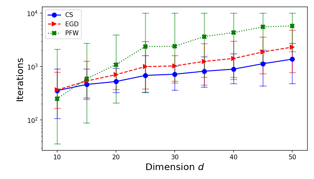
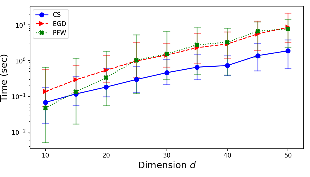
5.1 Projection onto the Convex Hull

Projection onto a convex hull arises in many areas like machine learning [5, 6, 4], collision detection [41] and imaging [42, 43]. It involves finding a point in the convex hull of a set of points $\{x_{i}\}_{1\leq i\leq n}$, with $x_{i}\in\mathbb{R}^{d}$, that is closest to an arbitrary point $y\in\mathbb{R}^{d}$, i.e.,

$$\min_{w}\|wX-y\|^{2}\qquad\textrm{where}\qquad\sum_{i}w_{i}=1\ \textrm{and}\ w_{i}\geq 0,$$ (35)

and $X=[x_{1},\cdots,x_{n}]^{T}$ is a $\mathbb{R}^{n\times d}$ matrix. This is also known as simplex-constrained regression.

Experimental Details: We look at a convex hull sampled from the unit hypercube $[0,1]^{d}$ for $d\in[10,15,\ldots,50]$. For each hypercube, we sample 50 points uniformly on each of its surfaces, giving a convex hull $X$ with $n=100d$ data points.

Once $X$ is sampled, 50 $y$’s are created outside the hypercube perpendicular to a surface and unit length away from it. This is done by considering the 50 points in $X$ lying on a randomly selected surface of the hypercube. A point $y_{\text{true}}$ is created as a random convex combination of these points. The point $y$ can then be created perpendicular to this surface and a unit length away from $y_{\text{true}}$, and thus also from the convex hull of $X$.

Each $y$ is then projected onto $X$ using CS, EGD, and PFW. These algorithms are ran until a solution, $\hat{y}$, is found such that $\|\hat{y}-y_{\text{true}}\|\leq 1e^{-5}$ or $10\,000$ iterations have been made. We do not implement PGD and Frank-Wolfe due to their inefficiency in practice.

Implementation Details: The learning rate for EGD, PFW, and CS is found through a line search. In the case of the PFW and CS algorithms, an explicit solution can be found and used. At the same time, EGD implements a back-tracking linear search with Armijo conditions [38] to find an approximate solution.

Experiments were written in Python and ran on Google Colab. The code can be found on GitHub333https://github.com/infamoussoap/ConvexHull. The random data is seeded for reproducibility.

Results: The results can be seen in Fig. 1. For $d=10$, we see that PFW outperforms both CS and EGD in terms of the number of iterations required and the time taken. But for $d>10$, on average, CS converges with the least iterations and time taken.

Refer to caption
(a) Average steps taken in log-scale
Refer to caption
(b) Average time taken in log-scale
Figure 1: Number of steps and time required for PFW, EGD, and CS to project 50 randomly sampled points onto the $d$-hypercube. The bars indicate the minimum and maximum values.

5.2 Optimal Question Weighting

It is often desirable that the distribution of exam marks matches a target distribution, but this rarely happens. Modern standardized tests (e.g. IQ exams) solve this problem by transforming the distribution of the raw score of a given age group so it fits a normal distribution [44, 45, 46].

While IQ exams have many criticisms [47, 48, 49], we are interested in the raw score. As noted by Gottfredson and Linda S. [46], the raw score has no intrinsic meaning as it can be boosted by adding easier questions to the test. We also argue it is hard to predict the difficulty of a question relative to an age group and, thus, even harder to give it the correct weight. Hence making the raw score a bad reflection of a person’s performance.

Here we propose a framework to find an optimum weighting of questions such that the weighted scores will fit a target distribution. A demonstration can be seen in Fig. 2.

Consider $d$ students taking an exam with $n$ true or false questions. For simplicity, assume that person $j$ getting question $i$ correct can be modeled as a random variable $\mathcal{X}_{i,j}$ for $i=1,\ldots,n$ and $j=1,\ldots,d$. Consider the discrete distribution of $X_{j}=\sum_{i}w_{i}{\mathcal{X}}_{i,j}$ for some $w\in\Delta^{n}$, the weighted mark of person $j$. This distribution can be approximated as continuous distribution,

$$\rho_{\varepsilon}(z)=\frac{1}{d}\sum_{j=1}^{d}\mu_{\varepsilon}(z-X_{j})\quad\text{with}\quad\mu_{\varepsilon}(x)=\frac{1}{\varepsilon}\mu(x/\varepsilon),$$ (36)

$\varepsilon>0$ and $\mu$ is a continuous probability distribution, i.e. $\mu\geq 0$ and $\int\mu(x)dx=1$. This is also known as kernel density estimation.

We want to minimize the distance between $\rho_{\varepsilon}$ and some target distribution $f$. A natural choice is the relative entropy,

$$\min_{w\in\Delta^{n}}D(\rho_{\varepsilon}|f)=\min_{w\in\Delta^{n}}\int\rho_{\varepsilon}(x)\log\left(\frac{\rho_{\varepsilon}(x)}{f(x)}\right)\,dx,$$ (37)

of which we take its Riemann approximation,

$\displaystyle\min_{w\in\Delta^{n}}\hat{D}(\rho_{\varepsilon}|f)=\min_{w\in\Delta^{n}}\sum_{k=1}^{M}\rho_{\varepsilon}(x_{k})\log\left(\frac{\rho_{\varepsilon}(x_{k})}{f(x_{k})}\right)(x_{k}-x_{k-1}),$ (38)

where $\{x_{k}\}_{0\leq k\leq M}$ is a partition of a finite interval $[a,b]$.

We remark that this problem is not convex, as $\mu$ cannot be chosen to be convex w.r.t $w$ and be a probability distribution.

Refer to caption
Figure 2: Optimal question weighting for (randomly generated) exam scores with 200 students and 75 questions. The setup follows the experimental details in Section 5.2. The kernel density estimate uses a truncated unit normal distribution with $\varepsilon=0.05$, and the target distribution is a truncated normal distribution with a mean of 0.5 and a standard deviation of 0.1. We take $w^{0}=(0.01,\ldots,0.01)$, and the Cauchy-Simplex is applied, with each step using a backtracking line search. The resulting weighted histogram and kernel density estimate is shown. The distribution of the weighted marks is shown on the top row, and its QQ plots against a normal distribution of mean 0.5 and a standard deviation of 0.1 are shown on the bottom row. At iterations 0, 5, and 20, the weighted scores have a mean of 0.499, 0.514, and 0.501, with standard deviations of 0.128, 0.124, and 0.109, respectively.

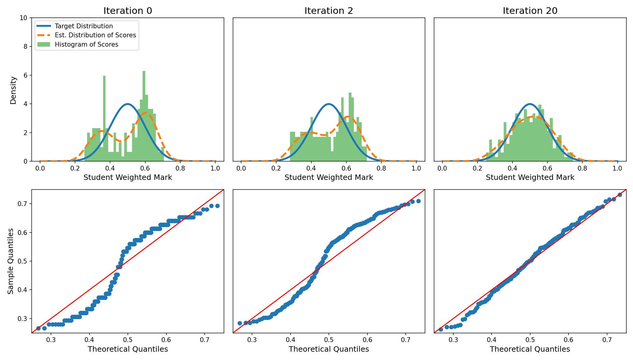
Experiment Details: We consider 25 randomly generated exam marks, each having $d=200$ students taking an exam with $n=75$ true or false questions. For simplicity, we assume that $\mathcal{X}_{i,j}\sim\text{Bernoulli}(q_{i}s_{j})$ where $0<q_{i}<1$ is the difficulty of question $i$ and $0<s_{j}<1$ the $j$-th student’s smartness.

For each scenario, $q_{i}=7/8$ for $1\leq i\leq 60$ and $q_{i}=1/5$ for $60<i\leq 75$, while $s_{j}=7/10$ for $1\leq j\leq 120$ and $s_{j}=1/2$ for $120<j\leq 200$. ${\mathcal{X}}_{i,j}\sim\text{Bernoulli}(q_{i}s_{j})$ are then sampled. This setup results in a bimodal distribution, with an expected average of $0.532$ and an expected standard deviation of $0.1206$, as shown in Figure 2.

For the kernel density estimate, $\mu(x)$ is chosen as a unit normal distribution truncated to $[0,1]$, with smoothing parameter $\varepsilon=0.05$. Similarly, $f$ is a normal distribution with mean $0.5$ and variance $0.1$, truncated to $[0,1]$. We take the partition $\{k/400\}_{0\leq k\leq 400}$ for the Riemann approximation.

The algorithms CS, EGD, and PFW are ran for 150 iterations.

Implementation Details: The learning rate for EGD, PFW, and CS is found through a line search. However, explicit solutions are not used. Instead, a back-tracking line search with Armijo conditions is used to find an approximate solution.

Experiments were written in Python and ran on Google Colab and can be found on GitHub444https://github.com/infamoussoap/ConvexHull. The random data is seeded for reproducibility.

Results: A table with the results can be seen in Table 2. In summary, of the 25 scenarios, PFW always produces solutions with the smallest relative entropy, with CS producing the largest relative entropy 13 times and EGD 12 times. For the time taken to make the 150 steps, PFW is the quickest 15 times, EGD 7 times, and CS 3 times. At the same time, EGD is the slowest 13 times, CS 7 times, and PFW 5 times.

It is perhaps expected that PFW outperforms both EGD and CS due to the low dimensionality of this problem. However, the CS produces similar relative entropies to EGD while maintaining a lower average run time of 5.22 seconds compared to the average run time of 5.68 sec for EGD.

Table 2: Results for optimal question weighting after running CS, EGD, and PFW for 150 iterations. The final distance (relative entropy) and the time taken in seconds are shown. Bold represents the minimum (best) value, and underline represents the maximum (worst) value.
CS EGD PFW
Trial Distance Time Distance Time Distance Time
1 0.032432 8.14 0.032426 10.98 0.032114 6.02
2 0.010349 5.95 0.010535 5.08 0.010101 4.46
3 0.016186 5.74 0.016252 4.93 0.015848 5.50
4 0.025684 4.62 0.025726 6.19 0.025309 4.51
5 0.020561 4.63 0.020486 6.03 0.020213 4.50
6 0.016559 5.58 0.016514 5.00 0.016287 4.52
7 0.025957 5.42 0.025867 4.87 0.025757 5.38
8 0.014506 4.77 0.014343 6.14 0.013504 4.28
9 0.032221 4.68 0.032412 6.02 0.032028 4.55
10 0.023523 5.59 0.023528 4.92 0.023232 5.34
11 0.016153 4.93 0.016231 5.01 0.015792 5.63
12 0.035734 4.53 0.035738 6.07 0.035212 4.22
13 0.030205 4.53 0.030234 6.13 0.029859 4.37
14 0.021725 5.80 0.021598 4.99 0.021282 5.85
15 0.030026 4.44 0.029982 4.99 0.029751 5.64
16 0.009212 4.75 0.009182 5.94 0.008931 4.27
17 0.015573 5.22 0.015661 5.46 0.015188 4.48
18 0.017681 5.69 0.017618 4.92 0.017321 5.48
19 0.017888 4.64 0.017874 5.34 0.017283 5.11
20 0.013597 4.55 0.013719 6.04 0.013075 4.42
21 0.016933 5.76 0.016780 4.84 0.016687 4.77
22 0.032185 5.80 0.032141 5.03 0.032039 6.03
23 0.018377 4.69 0.018250 6.06 0.018084 4.54
24 0.031167 4.59 0.031211 6.10 0.030820 4.55
25 0.035608 5.46 0.035674 4.98 0.035408 5.98
Average 5.22 5.68 4.97

5.3 Prediction from Expert Advice

Consider $N$ ‘experts’ (e.g., Twitter) who give daily advice for $1\leq t\leq T$. Suppose that, as a player in this game, taking advice from expert $i$ on the day $t$ will incur a loss $l^{t}_{i}\in[0,1]$. This loss is not known beforehand, only once the advice has been taken. The weighted loss $w^{t}\cdot l^{t}$ is the expected loss if we pick our expert w.r.t some distribution $w^{t}\in\Delta^{N}$. This problem is also known as the multi-armed bandit problem.

A simple goal is to generate a sequence of weight vectors $\{w^{t}\}_{t}$ to minimize the averaged expected loss. This goal is, however, a bit too ambitious as the loss vectors $l^{t}$ are not known beforehand. An easier problem is to find a sequence, $\{w^{t}\}_{t}$, such that its averaged expected loss approaches the average loss of the best expert as $T\to\infty$, that is

$\displaystyle\frac{1}{T}R_{T}\to 0,\quad\text{where}\quad R_{T}=\sum_{t=1}^{T}w^{t}\cdot l^{t}-\min_{i}\sum_{t=1}^{T}l^{t}_{i}$ (39)

as $T\to\infty$. $R_{T}$ is commonly known as the regret of the strategy $\{w^{t}\}_{t}$.

Previous works [50, 51, 52, 53] all yield $\mathcal{O}(\sqrt{T\log N})$ convergence rate for the regret.

Theorem 5.

Consider a sequence of adversary loss vectors $l^{t}\in[0,1]^{N}$. For any $u\in\Delta^{N}$, the regret generated by the Cauchy-Simplex scheme

$\displaystyle w^{t+1}=w^{t}(1-\eta_{t}\Pi_{w^{t}}\nabla f^{t})\quad\text{where}\quad\nabla f^{t}=l^{t},$ (40)

is bounded by

$\displaystyle\sum_{t=1}^{T}w^{t}\cdot l^{t}-\sum_{t=1}^{T}u\cdot l^{t}\leq\frac{D(u|w^{1})}{\eta}+\frac{T\eta}{2(1-\eta)},$ (41)

for a fixed learning rate $\eta_{t}=\eta<1$.

In particular, taking $w^{1}=(1/N,\ldots,1/N)$ and $\eta=\frac{\sqrt{2\log(N)}}{\sqrt{2\log(N)}+\sqrt{T}}$ gives the bound

$\displaystyle\sum_{t=1}^{T}w^{t}\cdot l^{t}-\sum_{t=1}^{T}u\cdot l^{t}$ $\displaystyle\leq$ $\displaystyle\sqrt{2T\log(N)}+\log(N).$ (42)

Moreover, this holds when $u=e_{j}$, where $j$ is the best expert and $e_{j}$ is the standard basis vector.

5.4 Universal Portfolio

Consider an investor with a fixed-time trading horizon, $T$, managing a portfolio of $N$ assets. Define the price relative for the $i$-th stock at time $t$ as $x^{t}_{i}=C^{t}_{i}/C^{t-1}_{i}$, where $C^{t}_{i}$ is the closing price at time $t$ for the $i$-th stock. So today’s closing price of asset $i$ equals $x_{i}^{t}$ times yesterday’s closing price, i.e. today’s price relative to yesterday’s.

A portfolio at day $t$ can be described as $w^{t}\in\Delta^{N}$, where $w_{i}^{t}$ is the proportion of an investor’s total wealth in asset $i$ at the beginning of the trading day. Then the wealth of the portfolio at the beginning of day $t+1$ is $w^{t}\cdot x^{t}$ times the wealth of the portfolio at day $t$.

Consider the average log-return of the portfolio

$\displaystyle\frac{1}{T}\log\left(\prod_{t=1}^{T}w^{t}\cdot x^{t}\right)=\frac{1}{T}\sum_{t=1}^{T}\log(w^{t}\cdot x^{t}).$ (43)

Similarly to predicting with expert advice, it is too ambitious to find a sequence of portfolio vectors $\{w^{t}\}_{t}$ that maximizes the average log-return. Instead, we wish to find such a sequence that approaches the best fixed-weight portfolio, i.e.

$\displaystyle\frac{1}{T}LR_{T}\to 0,\quad\text{where}\quad LR_{T}=\sum_{t=1}^{T}\log(u\cdot x^{t})-\sum_{t=1}^{T}\log(w^{t}\cdot x^{t})$ (44)

as $T\to\infty$, for some $u\in\Delta^{N}$. If such a sequence can be found, $\{w^{t}\}_{t}$ is a universal portfolio. $LR_{T}$ is commonly known as the log-regret.

Two standard assumptions are made when proving universal portfolios: (1) For every day, all assets have a bounded price relative, and at least one is non-zero, i.e. $0<\max_{i}x^{t}_{i}<\infty$ for all $t$, and (2) No stock goes bankrupt during the trading period, i.e. $a:=\min_{i,t}x_{i}^{t}>0$, where $a$ known as the market variability parameter. This is also known as the no-junk-bond assumption.

Over the years, various bounds on the log-regret have been proven under both assumptions. Some examples include Cover, in his seminal paper [54], with $\mathcal{O}(\log T)$, Helmbold et al. [3] with $\mathcal{O}(\sqrt{T\log N})$, Agarwal et al. [55] with $\mathcal{O}(N^{1.5}\log(NT))$, Hazan and Kale [56] with $\mathcal{O}(N\log(T+N))$, and Gaivoronski and Stella [57] with $\mathcal{O}(C^{2}\log(T))$ where $C=\sup_{x\in\Delta^{N}}\|\nabla_{b}\log(b\cdot x)\|$ and adding an extra assumption on independent price relatives. Each with varying levels of computational complexity.

Remark 5.

Let $x^{t}\in[a,b]^{N}$ be a bounded sequence of price relative vectors for $0\leq a\leq b<\infty$. Since the log-regret is invariant under re-scalings of $x^{t}$, w.l.o.g. we can look at the log-regret for the re-scaled return vectors $x^{t}\in[\tilde{a},1]^{N}$ for $0\leq\tilde{a}\leq 1$.

Theorem 6.

Consider a bounded sequence of price relative vectors $x^{t}\in[a,1]^{N}$ for some positive constant $0<a\leq 1$, and $\max_{i}x_{i}^{t}=1$ for all $t$. Then the log-regret generated by the Cauchy-Simplex

$\displaystyle w^{t+1}=w^{t}(1-\eta\Pi_{w^{t}}\nabla f^{t}),\quad\text{where}\quad\nabla f^{t}=-\frac{x^{t}}{w^{t}\cdot x^{t}},$ (45)

is bounded by

$\displaystyle\sum_{t=1}^{T}\log(u\cdot x^{t})-\sum_{t=1}^{T}\log(w^{t}\cdot x^{t})\leq\frac{D(u|w^{1})}{\eta}+\frac{T\eta}{2a^{2}(1-\eta)},$ (46)

for any $u\in\Delta^{N}$ and $0<\eta\leq 1$.

In particular, taking $w^{1}=(1/N,\ldots,1/N)$ and $\eta=\frac{a\sqrt{2\log(N)}}{a\sqrt{2\log(N)}+\sqrt{T}}$ gives the bound

$\displaystyle\sum_{t=1}^{T}\log(u\cdot l^{t})-\sum_{t=1}^{T}\log(w^{t}\cdot l^{t})\leq\frac{\sqrt{2T\log(N)}}{a}+\log(N).$ (47)

Experimental Details: We look at the performance of our algorithm on four standard datasets used to study the performance of universal portfolios: (1) NYSE is a collection of 36 stocks traded on the New York Stock Exchange from July 3, 1962, to Dec 31, 1984, (2) DJIA is a collection of 30 stocks tracked by the Dow Jones Industrial Average from Jan 14, 2009, to Jan 14, 2003, (3) SP500 is a collection of the 25 largest market cap stocks tracked by the Standard & Poor’s 500 Index from Jan 2, 1988, to Jan 31, 2003, and (4) TSE is a collection of 88 stocks traded on the Toronto Stock Exchange from Jan 4, 1994, to Dec 31, 1998.555The datasets were original found on http://www.cs.technion.ac.il/~rani/portfolios/, but is now unavailable. It was retrieved using the WayBack Machine https://web.archive.org/web/20220111131743/http://www.cs.technion.ac.il/~rani/portfolios/.

Two other portfolio strategies are considered: (1) Helmbold et. al. [3] (EGD), who uses the EGD scheme $w^{t+1}=w^{t}\exp(\eta\nabla f^{t})/\sum_{i}w^{t}_{i}\exp(\eta\nabla_{i}f^{t})$, with $\nabla f^{t}=x^{t}/w^{t}\cdot x^{t}$, and (2) Buy and Hold (B&H) strategy, where one starts with an equally weighted portfolio and the portfolio is left to its own devices.

Two metrics are used to evaluate the performance of the portfolio strategies: (1) The Annualized Percentage Yield: $\text{APY}=\text{R}^{1/y}-1$, where $R$ is the total return over the full trading period, and $y=T/252$, where 252 is the average number of annual trading days, and (2) The Sharpe Ratio: $\text{SR}=(\text{APY}-R_{f})/\sigma$, where $\sigma^{2}$ is the variance of the daily returns of the portfolio, and $R_{f}$ is the risk-free interest rate. Intuitively, the Sharpe ratio measures the performance of the portfolio relative to a risk-free investment while also factoring in the portfolio’s volatility. Following [58], we take $R_{f}=4\%$.

We take the learning rate as the one used to prove that CS and EGD are universal portfolios. In particular, $\eta_{\text{CS}}=\frac{a\sqrt{2\log N}}{a\sqrt{2\log N}+\sqrt{T}}$ and $\eta_{\text{EGD}}=2a\sqrt{2\log(N)/T}$, respectively, where $a$ is the market variability parameter. We assume that the market variability parameter is given for each dataset.

Experiments were written in Python and can be found on GitHub666https://github.com/infamoussoap/UniversalPortfolio.

Results: A table with the results can be seen in Table 3. For the NYSE, DJIA, and SP500 datasets, CS slightly outperforms EGD in both the APY and Sharpe ratio, with EGD having a slight edge on the APY for the NYSE dataset. But curiously, the B&H strategy outperforms both CS and EGD on the TSE.

We remark that this experiment does not reflect real-world performance, as the market variability parameter is assumed to be known, transaction costs are not factored into our analysis, and the no-junk-bond assumption tends to overestimate performance [59, 60, 61]. However, this is outside of the scope of this paper. It is only shown as a proof of concept.

Table 3: Performance of different portfolio strategies on different datasets. Bold represents the maximum (best) value, and underline represents the minimum (worst) value.
CS EGD B&H
Dataset APY Sharpe APY Sharpe APY Sharpe
NYSE 0.162 14.360 0.162 14.310 0.129 9.529
DJIA -0.099 -8.714 -0.101 -8.848 -0.126 -10.812
SP500 0.104 4.595 0.101 4.395 0.061 1.347
TSE 0.124 10.225 0.123 10.204 0.127 10.629

6 Conclusion

This paper presents a new iterative algorithm, the Cauchy-Simplex, to solve convex problems over a probability simplex. Within this algorithm, we find ideas from previous works which only capture a portion of the simplex constraint. Combining these ideas, the Cauchy-Simplex provides a numerically efficient framework with nice theoretical properties.

The Cauchy-Simplex maintains the linear form of Projected Gradient Descent, allowing one to find analytical solutions to a line search for certain convex problems. But unlike projected gradient descent, this analytical solution will remain in the probability simplex. A backtracking line search can be used when an analytical solution cannot be found. However, this requires an extra parameter, the maximum candidate step size. The Cauchy-Simplex provides a natural answer as a maximum learning rate is required to enforce positivity, rather than the exponentials used in Exponentied Gradient Descent.

Since the Cauchy-Simplex satisfies both constraints of the probability simplex in its iteration scheme, its gradient flow can be used to prove convergence for differentiable and convex functions. This implies the convergence of its discrete linear scheme. This is in contrast to EGD, PFW, and PGD, in which its discrete nature is crucial in satisfying both constraints of the probability simplex. More surprisingly, we find that in the proofs, formulas natural to probability, i.e., variance, and relative entropy, are necessary when proving convergence.

We believe that the strong numerical results and simplicity seen through its motivating derivation, gradient flow, and iteration scheme make it a strong choice for solving problems with a probability simplex constraint.

Appendix A Convergence Proofs

We will use the notation $\Pi^{t}=\Pi_{w_{t}}$ and $\nabla f^{t}=\nabla f(w^{t})$ for the remaining section.

A.1 Decreasing Relative Entropy

Theorem 7.

For any $u\in\Delta^{N}$, each iteration of the linear Cauchy-Simplex (7) satisfies the bound

$\displaystyle D(u|w^{t+1})-D(u|w^{t})\leq\eta_{t}u\cdot(\Pi^{t}\nabla f^{t})+C_{\gamma_{t}}\eta_{t}^{2}u\cdot(\Pi^{t}\nabla f^{t})^{2},$ (48)

where $C_{\gamma_{t}}=\gamma_{t}^{-2}\log(e^{-\gamma_{t}}/(1-\gamma_{t}))$ and $\eta_{t}=\gamma_{t}\eta_{t,\max}$ with $\gamma_{t}\in(0,1)$.

Proof.

By direct computation

$\displaystyle D(u|w^{t+1})-D(u|w^{t})$ $\displaystyle=$ $\displaystyle\sum_{i}u_{i}\log\left(\frac{1}{1-\eta_{t}\Pi^{t}\nabla_{i}f^{t}}\right)$ (49)
$\displaystyle=$ $\displaystyle\sum_{i}u_{i}\log\left(\frac{e^{-\eta_{t}\Pi^{t}\nabla_{i}f^{t}}}{1-\eta_{t}\Pi^{t}\nabla_{i}f^{t}}e^{\eta_{t}\Pi^{t}\nabla_{i}f^{t}}\right)$ (50)
$\displaystyle=$ $\displaystyle\eta_{t}u\cdot(\Pi^{t}\nabla f^{t})+\sum_{i}u_{i}\log\left(\frac{e^{-\eta_{t}\Pi^{t}\nabla_{i}f^{t}}}{1-\eta_{t}\Pi^{t}\nabla_{i}f^{t}}\right).$ (51)

Since the learning rate can be written as $\eta_{t}=\gamma_{t}\eta_{t,\max}$, with $\gamma_{t}\in(0,1)$,

$\displaystyle\eta_{t}\Pi^{t}\nabla_{i}f^{t}\leq(\gamma_{t}\eta_{t,\max})\max_{i}\Pi^{t}\nabla_{i}f^{t}=\gamma_{t}<1.$ (52)

Consider the inequality $0\leq\log(e^{-x}/(1-x))\leq C_{\gamma_{t}}\,x^{2}$ for $x<\gamma_{t}$ and $C_{\gamma_{t}}=\gamma_{t}^{-2}\log(e^{-\gamma_{t}}/(1-\gamma_{t}))$. Note that $C_{\gamma_{t}}\geq 0$ for $\gamma_{t}\in[0,1]$ and $C_{\gamma_{t}}\to\infty$ as $\gamma_{t}\to 1$. Therefore,

$\displaystyle 0\leq\log\left(\frac{e^{-\eta_{t}\Pi^{t}\nabla_{i}f^{t}}}{1-\eta_{t}\Pi^{t}\nabla_{i}f^{t}}\right)\leq C_{\gamma_{t}}\eta_{t}^{2}(\Pi^{t}\nabla_{i}f^{t})^{2}.$ (53)

Giving the required inequality

$\displaystyle D(u|w^{t+1})-D(u|w^{t})$ $\displaystyle\leq$ $\displaystyle\eta_{t}u\cdot(\Pi^{t}\nabla f^{t})+C_{\gamma_{t}}\eta_{t}^{2}u\cdot(\Pi^{t}\nabla f^{t})^{2}.$ (54)

A.2 Proof of Theorem 4

Proof.

By Theorem 7,

$\displaystyle D(w^{*}|w^{t+1})-D(w^{*}|w^{t})$ $\displaystyle\leq$ $\displaystyle\eta_{t}\nabla f^{t}\cdot(w^{*}-w^{t})+C_{\gamma_{t}}\eta_{t}^{2}w^{*}\cdot(\Pi^{t}\nabla f^{t})^{2}.$ (55)

By convexity of $f$, rearranging gives

$\displaystyle\eta_{t}\big{(}f(w^{t})-f(w^{*})\big{)}\leq D(w^{*}|w^{t})-D(w^{*}|w^{t+1})+C_{\gamma_{t}}\eta_{t}^{2}w^{*}\cdot(\Pi^{t}\nabla f^{t})^{2}.$ (56)

By Theorem 8, we have that

$\displaystyle f(w^{t})\geq f(w^{t+1})+\frac{\eta_{t}}{2}w^{t}\cdot(\Pi^{t}\nabla f^{t})^{2}.$ (57)

Repeatedly applying this inequality gives

$\displaystyle f(w^{T})+\frac{1}{2}\sum_{k=t}^{T-1}\eta_{k}w^{k}\cdot(\Pi^{k}\nabla f^{k})^{2}\leq f(w^{t}),$ (58)

for $t\leq T-1$. Thus, (56) gives the bound

$\displaystyle\eta_{t}(f(w^{T})-f(w^{*}))\leq D(w^{*}|w^{t})$ $\displaystyle-$ $\displaystyle D(w^{*}|w^{t+1})+C_{\gamma_{t}}\eta_{t}^{2}w^{*}\cdot(\Pi^{t}\nabla f^{t})^{2}$
$\displaystyle-\frac{1}{2}\eta_{t}\sum_{k=t}^{T-1}\eta_{k}w^{k}\cdot(\Pi^{k}\nabla f^{k})^{2}.$

Summing over time and collapsing the sum gives

$\displaystyle(f(w^{T})-f(w^{*}))\sum_{t=0}^{T-1}\eta_{t}\leq D(w^{*}|w^{0})$ $\displaystyle-$ $\displaystyle D(w^{*}|w^{T})$
$\displaystyle+\sum_{t=0}^{T-1}C_{\gamma_{t}}\eta_{t}^{2}w^{*}\cdot(\Pi^{t}\nabla f^{t})^{2}$
$\displaystyle-\frac{1}{2}\sum_{t=0}^{T-1}\sum_{k=t}^{T-1}\eta_{k}\eta_{t}w^{k}\cdot(\Pi^{k}\nabla f^{k})^{2}.$

We can rewrite the last term as

$\displaystyle\sum_{t=0}^{T-1}\sum_{k=t}^{T-1}\eta_{k}\eta_{t}w^{k}\cdot(\Pi^{k}\nabla f^{k})^{2}=\sum_{t=0}^{T-1}\sum_{k=0}^{t}\eta_{k}\eta_{t}w^{t}\cdot(\Pi^{t}\nabla f^{t})^{2}.$ (61)

Thus, the last two terms of (A.2) can be bounded by

$\displaystyle S$ $\displaystyle:=$ $\displaystyle\sum_{t=0}^{T-1}\eta_{t}\left(C_{\gamma_{t}}\eta_{t}w^{*}\cdot(\Pi^{t}\nabla f^{t})^{2}-\frac{1}{2}\sum_{k=0}^{t}\eta_{k}w^{t}\cdot(\Pi^{t}\nabla f^{t})^{2}\right)$ (62)
$\displaystyle\leq$ $\displaystyle\sum_{t=0}^{T-1}\eta_{t}^{2}\left(C_{\gamma_{t}}\max_{i}\,(\Pi^{t}\nabla f^{t})^{2}_{i}-\frac{t+1}{2}w^{t}\cdot(\Pi^{t}\nabla f^{t})^{2}\right),$ (63)

since $\{\eta_{t}\}_{t}$ is a decreasing sequence and $w^{*}\in\Delta^{n}$. By assumption,

$\displaystyle C_{\gamma_{t}}\leq\frac{(t+1)\ w^{t}\cdot(\Pi^{t}\nabla f^{t})^{2}}{2\max_{i}\,(\Pi^{t}\nabla f^{t})^{2}_{i}},$ (64)

thus $S\leq 0$, and (A.2) gives

$\displaystyle f(w^{T})-f(w^{*})\leq\frac{D(w^{*}|w^{0})-D(w^{*}|w^{T})}{T\eta_{T}}.$ (65)

Taking $w^{0}=(1/n,\ldots,1/n)$, then $D(u|w^{0})\leq\log(n)$ for all $u\in\Delta^{n}$. Since relative entropy is non-negative,

$\displaystyle f(w^{T})-f(w^{*})\leq\frac{\log(n)}{T\,\eta_{T}}.$ (66)

Theorem 8 (Linear Progress Bound).

Let $f$ be convex, differentiable, and $\nabla f$ is $L$-Lipschitz continuous. Then each iteration of the linear Cauchy-Simplex (7) guarantees

$$f(w^{t+1})\leq f(w^{t})-\frac{\eta_{t}}{2}\textrm{Var}[\nabla f^{t}\,|\,w^{t}],\quad\text{for}\quad\eta_{t}\leq\min\bigg{\{}\frac{1}{L},\eta_{t,\max}\bigg{\}},$$ (67)

where $\eta_{t,\max}$ is defined in (7).

Proof.

Since $f$ is convex with $\nabla f$ Lipshitz continuous, we have the inequality [62]

$$f(w^{t+1})\leq f(w^{t})+\nabla f^{t}\cdot(w^{t+1}-w^{t})+\frac{L}{2}\|w^{t+1}-w^{t}\|^{2}.$$ (68)

Our iteration scheme gives that

$$\|w^{t+1}-w^{t}\|^{2}=\eta_{t}^{2}\sum_{i}\Big{(}w^{t}_{i}\,\Pi^{t}\nabla_{i}f^{t}\Big{)}^{2}\leq\eta_{t}^{2}\sum_{i}w_{i}^{t}(\Pi^{t}\nabla_{i}f^{t})^{2},$$ (69)

since $0\leq w_{i}^{t}\leq 1$. Hence

$$f(w^{t+1})\leq f(w^{t})-\eta_{t}\textrm{Var}[\nabla f^{t}|w_{t}]+\eta_{t}^{2}\frac{L}{2}\text{Var}[\nabla f^{t}|w_{t}].$$ (70)

Minimizing the right side of this inequality with respect to $\eta_{t}$ gives that

$$f(w^{t+1})\leq f(w^{t})-\frac{\eta_{t}}{2}\textrm{Var}[\nabla f^{t}\,|\,w^{t}],\quad\text{for}\quad\eta_{t}\leq\min\bigg{\{}\frac{1}{L},\eta_{t,\max}\bigg{\}}.$$ (71)

A.3 Proof of Theorem 5

Proof.

Rearranging Theorem 7 gives

$\displaystyle-\eta_{t}u\cdot(\Pi^{t}\nabla f^{t})\leq D(u|w^{t})-D(u|w^{t+1})+C_{\gamma_{t}}\eta_{t}^{2}u\cdot(\Pi^{t}\nabla f^{t})^{2}.$ (72)

Since $\nabla f^{t}=l^{t}$, we have the inequality

$\displaystyle-1\leq\Pi^{t}\nabla_{i}f^{t}=l^{t}_{i}-w^{t}\cdot l^{t}\leq 1,$ (73)

as $l^{t}_{i}\in[0,1]$. Thus dividing (72) by $\eta_{t}$ gives

$\displaystyle w^{t}\cdot l^{t}-u\cdot l^{t}\leq\frac{D(u|w^{t})-D(u|w^{t+1})}{\eta_{t}}+C_{\gamma_{t}}\eta_{t},$ (74)

where $\eta_{t}=\gamma_{t}\eta_{t,\max}$, for some $\gamma_{t}\in(0,1)$.

Since the maximum learning rate has the lower bound

$\displaystyle\eta_{t,\max}=\frac{1}{\max_{i}l_{i}^{t}-w^{t}\cdot l^{t}}\geq\frac{1}{\max_{i}l^{t}_{i}}\geq 1,$ (75)

we can take a fixed learning rate $\eta_{t}=\eta\in(0,1)$. Moreover, $\gamma_{t}=\eta/\eta_{t,\max}\leq\eta$. Since $C_{\gamma_{t}}$ is an increasing function of $\gamma_{t}$, $C_{\gamma_{t}}\leq C_{\eta}$, thus giving the bound

$\displaystyle w^{t}\cdot l^{t}-u\cdot l^{t}\leq\frac{D(u|w^{t})-D(u|w^{t+1})}{\eta}+C_{\eta}\eta.$ (76)

Summing over time and collapsing the sum gives the bound

$\displaystyle\sum_{t=1}^{T}w^{t}\cdot l^{t}-\sum_{t=1}^{T}u\cdot l^{t}$ $\displaystyle\leq$ $\displaystyle\frac{D(u|w^{1})-D(u|w^{T+1})}{\eta}+TC_{\eta}\eta$ (77)
$\displaystyle\leq$ $\displaystyle\frac{D(u|w^{1})}{\eta}+TC_{\eta}\eta$ (78)
$\displaystyle=$ $\displaystyle\frac{D(u|w^{1})}{\eta}+\frac{T\log(e^{-\eta}/(1-\eta))}{\eta},$ (79)

by definition of $C_{\eta}$. Using the inequality $\log(e^{-x}/(1-x))/x\leq x/(2(1-x))$ for $0\leq x\leq 1$,

$\displaystyle\sum_{t=1}^{T}w^{t}\cdot l^{t}-\sum_{t=1}^{T}u\cdot l^{t}$ $\displaystyle\leq$ $\displaystyle\frac{D(u|w^{1})}{\eta}+\frac{T\eta}{2(1-\eta)}.$ (80)

Let $w^{1}=(1/N,\ldots,1/N)$, then $D(u|w^{1})\leq\log(N)$ for all $u\in\Delta^{N}$. Thus giving the desired bound

$\displaystyle\sum_{t=1}^{T}w^{t}\cdot l^{t}-\sum_{t=1}^{T}u\cdot l^{t}$ $\displaystyle\leq$ $\displaystyle\frac{\log(N)}{\eta}+\frac{T\eta}{2(1-\eta)}.$ (81)

The right side of this inequality is minimized when $\eta=\frac{\sqrt{2\log(N)}}{\sqrt{2\log(N)}+\sqrt{T}}<1$. Upon substitution gives the bound

$\displaystyle\sum_{t=1}^{T}w^{t}\cdot l^{t}-\sum_{t=1}^{T}u\cdot l^{t}$ $\displaystyle\leq$ $\displaystyle\sqrt{2T\log(N)}+\log(N).$ (82)

A.4 Proof of Theorem 6

Proof.

Rearranging Theorem 7 gives

$\displaystyle-\eta_{t}u\cdot(\Pi^{t}\nabla f^{t})\leq D(u|w^{t})-D(u|w^{t+1})+C_{\gamma_{t}}\eta_{t}^{2}u\cdot(\Pi^{t}\nabla f^{t})^{2}.$ (83)

Since $\nabla f=-x^{t}/(w^{t}\cdot x^{t})$, we have the inequality

$\displaystyle-\frac{1}{a}\leq\Pi\nabla_{i}f=1-x_{i}^{t}/(w^{t}\cdot x^{t})\leq 1,$ (84)

as $x^{t}_{i}\in[{a},1]$. Thus diving by $\eta_{t}$ gives the bound

$\displaystyle\frac{u\cdot x^{t}}{w^{t}\cdot x^{t}}-1\leq\frac{D(u|w^{t})-D(u|w^{t+1})}{\eta_{t}}+\frac{C_{\gamma}\eta_{t}}{a^{2}}.$ (85)

Using the inequality $e^{x}-1\geq x$ for all $x$ gives

$\displaystyle\log\left(\frac{u\cdot x^{t}}{w^{t}\cdot x^{t}}\right)\leq\frac{D(u|w^{t})-D(u|w^{t+1})}{\eta_{t}}+\frac{C_{\gamma}\eta_{t}}{a^{2}}.$ (86)

Since the maximum learning rate has the lower bound

$\displaystyle\eta_{t,\max}=\frac{1}{\max_{i}(1-x^{t}_{i}/w^{t}\cdot x^{t})}=\frac{1}{1-\min_{i}(x^{t}_{i}/w^{t}\cdot x^{t})}\geq 1,$ (87)

we can take a fixed learning rate $\eta_{t}=\eta$.

Following the steps from Theorem 5 gives the bound

$\displaystyle\sum_{t=1}^{T}\log(u\cdot l^{t})-\sum_{t=1}^{T}\log(w^{t}\cdot l^{t})\leq\frac{D(u|w^{1})}{\eta}+\frac{T\eta}{2a^{2}(1-\eta)}.$ (88)

Taking $w^{1}=(1/N,\ldots,1/N)$ and minimizing the right-hand side of the inequality w.r.t $\eta$ gives $\eta=\frac{a\sqrt{2\log(N)}}{a\sqrt{2\log(N)}+\sqrt{T}}$. Thus giving the bound

$\displaystyle\sum_{t=1}^{T}\log(u\cdot l^{t})-\sum_{t=1}^{T}\log(w^{t}\cdot l^{t})\leq\frac{\sqrt{2T\log(N)}}{a}+\log(N).$ (89)

Appendix B Karush-Kuhn-Tucker Conditions

The Karush-Kuhn-Tucker (KKT) Conditions are first-order conditions that are necessary but insufficient for optimality in constrained optimization problems. For convex problems, it becomes a sufficient condition for optimality.

Consider a general constrained optimization problem

$\displaystyle\min_{w}f(w)\qquad\textrm{s.t.}\qquad g_{i}(w)\leq 0\quad\textrm{and}\quad h_{j}(w)=0,$ (90)

for $i=1,...,n$ and $j=1,...,m$. The (primal) Lagrangian is defined as

$\displaystyle\mathcal{L}(w,\alpha,\beta)=f(w)+\sum_{i}\alpha_{i}g_{i}(w)+\sum_{j}\beta_{j}h_{j}(w).$ (91)

Consider the new optimization problem

$\displaystyle\theta(w)=\max_{\alpha,\beta;\ \alpha_{i}\geq 0}\mathcal{L}(w,\alpha,\beta).$ (92)

Note that

$\displaystyle\theta(w)=\begin{cases}f(w)\qquad&\textrm{if $w$ satisfies the constraints}\\ 0\qquad&\textrm{otherwise}.\end{cases}$ (93)

Hence, $\alpha_{i}$ and $\beta_{j}$ are slack variables that render a given Lagrangian variation equation irrelevant when violated.

To solve (90), we can instead consider the new optimization problem

$\displaystyle\min_{w}\theta(w)=\min_{w}\max_{\alpha,\beta;\ \alpha_{i}\geq 0}\mathcal{L}(w,\alpha,\beta).$ (94)

Assume $f$ and $g_{i}$ are convex, $h_{j}$ is affine, and the constraints are feasible. A solution $(w^{*},\alpha^{*},\beta^{*})$ is an optimal solution to (90) if the following conditions, known as the KKT conditions, are satisfied:

$\displaystyle\frac{\partial}{\partial w_{i}}\mathcal{L}(w^{*},\alpha^{*},\beta^{*})$ $\displaystyle=$ $\displaystyle\ 0\qquad\text{(Stationarity)}$ (95)
$\displaystyle\alpha_{i}^{*}g_{i}(w^{*})$ $\displaystyle=$ $\displaystyle\ 0\qquad\text{(Complementary Slackness)}$ (96)
$\displaystyle g_{i}(w^{*})\ \leq\ 0,\ h_{j}(w)$ $\displaystyle=$ $\displaystyle\ 0\qquad\text{(Primal Feasibility)}$ (97)
$\displaystyle\alpha_{i}^{*}$ $\displaystyle\geq$ $\displaystyle\ 0\qquad\text{(Dual Feasibility)},$ (98)

for all $i$ and $j$.

When the constraint is a simplex, the Lagrangian becomes

$\displaystyle\mathcal{L}(w,\alpha,\beta)=f(w)-\sum_{i}\alpha_{i}w_{i}+\beta\left(\sum_{i}w_{i}-1\right).$ (99)

Thus stationarity gives

$\displaystyle\frac{\partial}{\partial w_{i}}\mathcal{L}=\nabla_{i}f-\alpha_{i}+\beta=0.$ (100)

Let $Q=\{i:w_{i}=0\}$ be the active set and $S=\{i:w_{i}>0\}$ be the support. The complementary slackness requires $\alpha_{i}=0$ for $i\in S$, so stationarity gives $\beta=\nabla_{i}f$, i.e. constant on the support. The active set’s dual feasibility and stationarity conditions thus require $\alpha_{i}=\beta+\nabla_{i}f\geq 0$.

Acknowledgements

We thank Prof. Johannes Ruf for the helpful discussion and his suggestion for potential applications in the multi-armed bandit problem, which ultimately helped the proof for universal portfolios.

References

  • [1] T.-J. Chang, N. Meade, J.E. Beasley, and Y.M. Sharaiha. Heuristics for cardinality constrained portfolio optimisation. Computers & Operations Research, 27(13):1271–1302, 2000.
  • [2] Puja Das and Arindam Banerjee. Meta optimization and its application to portfolio selection. In Proceedings of the 17th ACM SIGKDD International Conference on Knowledge Discovery and Data Mining, KDD ’11, page 1163–1171, New York, NY, USA, 2011. Association for Computing Machinery.
  • [3] David P. Helmbold, Robert E. Schapire, Yoram Singer, and Manfred K. Warmuth. On-line portfolio selection using multiplicative updates. Mathematical Finance, 8(4):325–347, October 1998.
  • [4] Lori Ziegelmeier, Michael Kirby, and Chris Peterson. Stratifying high-dimensional data based on proximity to the convex hull boundary. SIAM Review, 59(2):346–365, 2017.
  • [5] A.P. Nemirko and J.H. Dulá. Machine learning algorithm based on convex hull analysis. Procedia Computer Science, 186:381–386, 2021. 14th International Symposium Intelligent Systems.
  • [6] Georgi Nalbantov, Patrick Groenen, and J.C. Bioch. Nearest convex hull classification. Erasmus University Rotterdam, Econometric Institute, Econometric Institute Report, 01 2006.
  • [7] Xiaofei Zhou and Yong Shi. Nearest neighbor convex hull classification method for face recognition. In International Conference on Computational Science, pages 570–577. Springer, 2009.
  • [8] Immanuel M. Bomze. Regularity versus degeneracy in dynamics, games, and optimization: A unified approach to different aspects. SIAM Review, 44(3):394–414, 2002.
  • [9] Peter Schuster and Karl Sigmund. Replicator dynamics. Journal of Theoretical Biology, 100(3):533–538, 1983.
  • [10] E. de Klerk, D. den Hertog, and G. Elabwabi. On the complexity of optimization over the standard simplex. European Journal of Operational Research, 191(3):773–785, 2008.
  • [11] Maximilian Amsler, Vinay I. Hegde, Steven D. Jacobsen, and Chris Wolverton. Exploring the high-pressure materials genome. Physical Review X, 8(4), nov 2018.
  • [12] Leonard E. Baum and J. A. Eagon. An inequality with applications to statistical estimation for probabilistic functions of Markov processes and to a model for ecology. Bulletin of the American Mathematical Society, 73(3):360 – 363, 1967.
  • [13] Antonina Kuznetsova and Alexander xStrekalovsky. On solving the maximum clique problem, 2001.
  • [14] Yunmei Chen and Xiaojing Ye. Projection onto a simplex, 2011.
  • [15] Weiran Wang and Miguel A. Carreira-Perpiñán, 2013.
  • [16] David G. Luenberger. Optimization by Vector Space Methods. John Wiley &amp; Sons, Inc., USA, 1st edition, 1997.
  • [17] Vidar Alstad and Sigurd Skogestad. Null space method for selecting optimal measurement combinations as controlled variables. Industrial & Engineering Chemistry Research, 46(3):846–853, 2007.
  • [18] Roozbeh Yousefzadeh. A sketching method for finding the closest point on a convex hull, 2021.
  • [19] Philip E. Gill, Walter Murray, and Margaret H. Wright. Practical Optimization. Society for Industrial and Applied Mathematics, Philadelphia, PA, 2019.
  • [20] Jorge Nocedal and Stephen J. Wright. Numerical Optimization. Springer, New York, NY, USA, 2e edition, 2006.
  • [21] A.S. Nemirovsky and D.B. Yudin. Problem Complexity and Method Efficiency in Optimization. A Wiley-Interscience publication. Wiley, 1983.
  • [22] Jyrki Kivinen and Manfred K. Warmuth. Exponentiated gradient versus gradient descent for linear predictors. Information and Computation, 132(1):1–63, 1997.
  • [23] Marguerite Frank and Philip Wolfe. An algorithm for quadratic programming. Naval Research Logistics Quarterly, 3(1-2):95–110, 1956.
  • [24] Aurélien Bellet, Yingyu Liang, Alireza Bagheri Garakani, Maria-Florina Balcan, and Fei Sha. A Distributed Frank-Wolfe Algorithm for Communication-Efficient Sparse Learning, pages 478–486. Society for Industrial and Applied Mathematics, 2015.
  • [25] Cun Mu, Yuqian Zhang, John Wright, and Donald Goldfarb. Scalable robust matrix recovery: Frank–wolfe meets proximal methods. SIAM Journal on Scientific Computing, 38(5):A3291–A3317, 2016.
  • [26] Kenya Tajima, Yoshihiro Hirohashi, Esmeraldo Ronnie Rey Zara, and Tsuyoshi Kato. Frank-Wolfe algorithm for learning SVM-type multi-category classifiers, pages 432–440. Society for Industrial and Applied Mathematics, 2021.
  • [27] Hua Ouyang and Alexander Gray. Fast Stochastic Frank-Wolfe Algorithms for Nonlinear SVMs, pages 245–256. Society for Industrial and Applied Mathematics, 2010.
  • [28] Simon Lacoste-Julien and Martin Jaggi. On the global linear convergence of frank-wolfe optimization variants, 2015.
  • [29] Immanuel. M. Bomze, Francesco Rinaldi, and Damiano Zeffiro. Frank-wolfe and friends: a journey into projection-free first-order optimization methods, 2021.
  • [30] Martin Jaggi. Revisiting Frank-Wolfe: Projection-free sparse convex optimization. In Sanjoy Dasgupta and David McAllester, editors, Proceedings of the 30th International Conference on Machine Learning, volume 28 of Proceedings of Machine Learning Research, pages 427–435, Atlanta, Georgia, USA, 17–19 Jun 2013. PMLR.
  • [31] Jacques GuéLat and Patrice Marcotte. Some comments on wolfe’s ‘away step’, May 1986.
  • [32] Immanuel M. Bomze. On standard quadratic optimization problems. Journal of Global Optimization, 13(4):369–387, 12 1998. Copyright - Kluwer Academic Publishers 1998; Last updated - 2021-09-11.
  • [33] Andrea Scozzari and Fabio Tardella. A clique algorithm for standard quadratic programming. Discrete Appl. Math., 156(13):2439–2448, jul 2008.
  • [34] Immanuel M. Bomze and Etienne De Klerk. Solving standard quadratic optimization problems via linear, semidefinite and copositive programming. Journal of Global Optimization, 24(2):163–185, 2002.
  • [35] Ivo Nowak. A new semidefinite programming bound for indefinite quadratic forms over a simplex. Journal of Global Optimization, 14(4):357–364, 1999.
  • [36] E. de Klerk and D. V. Pasechnik. A linear programming reformulation of the standard quadratic optimization problem. Journal of Global Optimization, 37(1):75–84, July 2006.
  • [37] Yurii NESTEROV. Global quadratic optimization on the sets with simplex structure. LIDAM Discussion Papers CORE 1999015, Universite catholique de Louvain, Center for Operations Research and Econometrics (CORE), February 1999.
  • [38] J. Frédéric Bonnans, Jean Charles Gilbert, Claude Lemaréchal, and Claudia A. Sagastizábal. Numerical Optimization: Theoretical and Practical Aspects (Universitext). Springer-Verlag, Berlin, Heidelberg, 2006.
  • [39] Josiah Willard Gibbs. Elementary Principles in Statistical Mechanics. Cambridge University Press, September 2010.
  • [40] E. T. Jaynes. Probability Theory: The Logic of Science. Cambridge University Press, 2003.
  • [41] Xiangfeng Wang, Junping Zhang, and Wenxing Zhang. The distance between convex sets with minkowski sum structure: application to collision detection. Computational Optimization and Applications, 77(2):465–490, July 2020.
  • [42] Yongyi Yang and N.P. Galatsanos. Removal of compression artifacts using projections onto convex sets and line process modeling. IEEE Transactions on Image Processing, 6(10):1345–1357, 1997.
  • [43] Seung-Won Jung, Tae-Hyun Kim, and Sung-Jea Ko. A novel multiple image deblurring technique using fuzzy projection onto convex sets. IEEE Signal Processing Letters, 16(3):192–195, 2009.
  • [44] Nicholas Mackintosh. IQ and Human Intelligence. Oxford University Press, London, England, 2 edition, March 2011.
  • [45] David J Bartholomew. Measuring intelligence. Cambridge University Press, Cambridge, England, August 2004.
  • [46] Linda S. Gottfredson. Logical fallacies used to dismiss the evidence on intelligence testing. In Correcting fallacies about educational and psychological testing., pages 31–32. American Psychological Association, 2009.
  • [47] Ken Richardson. What iq tests test. Theory & Psychology, 12(3):283–314, 2002.
  • [48] Ann B. Shuttleworth-Edwards, Ryan D. Kemp, Annegret L. Rust, Joanne G.L. Muirhead, Nigel P. Hartman, and Sarah E. Radloff. Cross-cultural effects on iq test performance: A review and preliminary normative indications on wais-iii test performance. Journal of Clinical and Experimental Neuropsychology, 26(7):903–920, 2004. PMID: 15742541.
  • [49] A. B. Shuttleworth-Edwards. Generally representative is representative of none: commentary on the pitfalls of iq test standardization in multicultural settings. The Clinical Neuropsychologist, 30(7):975–998, 2016. PMID: 27377008.
  • [50] Sanjeev Arora, Elad Hazan, and Satyen Kale. The multiplicative weights update method: a meta-algorithm and applications. Theory of Computing, 8(6):121–164, 2012.
  • [51] Yoav Freund and Robert E Schapire. A decision-theoretic generalization of on-line learning and an application to boosting. Journal of Computer and System Sciences, 55(1):119–139, 1997.
  • [52] N. Littlestone and M.K. Warmuth. The weighted majority algorithm. Information and Computation, 108(2):212–261, 1994.
  • [53] Nicolò Cesa-Bianchi, Yoav Freund, David Haussler, David P. Helmbold, Robert E. Schapire, and Manfred K. Warmuth. How to use expert advice. J. ACM, 44(3):427–485, may 1997.
  • [54] Thomas M. Cover. Universal portfolios. Mathematical Finance, 1(1):1–29, January 1991.
  • [55] Amit Agarwal, Elad Hazan, Satyen Kale, and Robert E. Schapire. Algorithms for portfolio management based on the newton method. In Proceedings of the 23rd international conference on Machine learning - ICML '06. ACM Press, 2006.
  • [56] Elad Hazan and Satyen Kale. An online portfolio selection algorithm with regret logarithmic in price variation. Mathematical Finance, 25(2):288–310, 2015.
  • [57] Alexei A. Gaivoronski and Fabio Stella. Stochastic nonstationary optimization for finding universal portfolios. Annals of Operations Research, 100(1/4):165–188, 2000.
  • [58] Bin Li, Peilin Zhao, Steven C. H. Hoi, and Vivekanand Gopalkrishnan. PAMR: Passive aggressive mean reversion strategy for portfolio selection. Machine Learning, 87(2):221–258, February 2012.
  • [59] E Gilbert and D Strugnell. Does survivorship bias really matter? an empirical investigation into its effects on the mean reversion of share returns on the JSE (1984–2007). Investment Analysts Journal, 39(72):31–42, January 2010.
  • [60] David H Bailey, Jonathan M Borwein, Marcos López de Prado, and Qiji Jim Zhu. Pseudomathematics and financial charlatanism: The effects of backtest over fitting on out-of-sample performance. Notices of the AMS, 61(5):458–471, 2014.
  • [61] David H. Bailey and Marcos Lopez de Prado. The deflated sharpe ratio: Correcting for selection bias, backtest overfitting and non-normality. SSRN Electronic Journal, 2014.
  • [62] Xingyu Zhou. On the fenchel duality between strong convexity and lipschitz continuous gradient, 2018.