Geometric Hitting Set for Line-Constrained Disks and Related Problems

Abstract

Given a set $P$ of $n$ weighted points and a set $S$ of $m$ disks in the plane, the hitting set problem is to compute a subset $P^{\prime}$ of points of $P$ such that each disk contains at least one point of $P^{\prime}$ and the total weight of all points of $P^{\prime}$ is minimized. The problem is known to be NP-hard. In this paper, we consider a line-constrained version of the problem in which all disks are centered on a line $\ell$. We present an $O((m+n)\log(m+n)+\kappa\log m)$ time algorithm for the problem, where $\kappa$ is the number of pairs of disks that intersect. For the unit-disk case where all disks have the same radius, the running time can be reduced to $O((n+m)\log(m+n))$. In addition, we solve the problem in $O((m+n)\log(m+n))$ time in the $L_{\infty}$ and $L_{1}$ metrics, in which a disk is a square and a diamond, respectively. Our techniques can also be used to solve other geometric hitting set problems. For example, given in the plane a set $P$ of $n$ weighted points and a set $S$ of $n$ half-planes, we solve in $O(n^{4}\log n)$ time the problem of finding a minimum weight hitting set of $P$ for $S$. This improves the previous best algorithm of $O(n^{6})$ time by nearly a quadratic factor.

1 Introduction

Let $S$ be a set of $m$ disks and $P$ be a set of $n$ points in the plane such that each point of $P$ has a weight. The hitting set problem on $S$ and $P$ is to find a subset $P_{opt}\subseteq P$ of minimum total weight so that each disk of $S$ contains a least one point of $P_{opt}$ (i.e, each disk is hit by a point of $P_{opt}$). The problem is NP-hard even if all disks have the same radius and all point weights are the same [9, 18, 21].

In this paper, we consider the line-constrained version of the problem in which centers of all disks of $S$ are on a line $\ell$ (e.g., the $x$-axis). To the best of our knowledge, this line-constrained problem was not particularly studied before. We give an algorithm of $O((m+n)\log(m+n)+\kappa\log m)$ time, where $\kappa$ is the number of pairs of disks that intersect. We also present an alternative algorithm of $O(nm\log(m+n))$ time. For the unit-disk case where all disks have the same radius, we give a better algorithm of $O((n+m)\log(m+n))$ time. We also consider the problem in $L_{\infty}$ and $L_{1}$ metrics (the original problem is in the $L_{2}$ metric), where a disk becomes a square and a diamond, respectively; we solve the problem in $O((m+n)\log(m+n))$ time in both metrics. The 1D case where all disks are line segments can also be solved in $O((m+n)\log(m+n))$ time. In addition, by a reduction from the element uniqueness problem, we prove an $\Omega((m+n)\log(m+n))$ time lower bound in the algebraic decision tree model even for the 1D case (even if all segments have the same length and all points of $P$ have the same weight). The lower bound implies that our algorithms for the unit-disk, $L_{\infty}$, $L_{1}$, and 1D cases are all optimal.

Hitting set is a fundamental problem that has attracted much attention in the literature. Many variations of the problem are intractable. One motivation of our study is to see to what extent the hitting set problem has efficient algorithms and how efficient we could make. Our problem may also have direct applications. For example, suppose a number of sensors are deployed along a line (e.g., a high way or a rail way); we need to determine locations to build base stations to communicate with sensors (each sensor has a range for communications and the base station must be located within its range). How to determine a minimum number of locations for base stations is exactly an instance of our problem.

Although the problems are line-constrained, our techniques can be utilized to solve various other geometric hitting set problems. If all disks of $S$ have the same radius and the set of disk centers is separated from $P$ by a line $\ell$, the problem is called line-separable unit-disk hitting set problem. Our algorithm for the line-constrained $L_{2}$ general case can be used to solve the problem in $O(nm\log(m+n))$ time or in $O((m+n)\log(m+n)+\kappa\log m)$ time, where $\kappa$ is the number of pairs of disks whose boundaries intersect in the side of $\ell$ that contains $P$. Interestingly, we can also employ the algorithm to tackle the following half-plane hitting set problem. Given in the plane a set $S$ of $m$ half-planes and a set $P$ of $n$ weighted points, find a subset of $P$ of minimum total weight so that each half-plane of $S$ contains at least one point of the subset. For the lower-only case where all half-planes are lower ones, Chan and Grant [5] gave an $O(m^{2}n(m+n))$ time algorithm. Notably, recognizing that a half-plane can be seen as a special unit disk with an infinite radius, our line-separable unit-disk hitting set algorithm can be applied to solve the problem in $O(nm\log(m+n))$ time or in $O(n\log n+m^{2}\log m)$ time. This improves the result of [5] by nearly a quadratic factor. For the general case where both upper and lower half-planes are present, Har-Peled and Lee [16] proposed an algorithm of $O(n^{6})$ time when $m=n$. Based on observations, we manage to reduce the problem to $O(n^{2})$ instances of the lower-only case problem and consequently solve the problem in $O(n^{3}m\log(m+n))$ time or in $O(n^{3}\log n+n^{2}m^{2}\log m)$ time using our lower-only case algorithm. The runtime is $O(n^{4}\log n)$ when $m=n$, which improves the one in [16] by nearly a quadratic factor. We believe that our techniques have the potential to find numerous other applications.

Related work.

The hitting set and many of its variations are fundamental and have been studied extensively; the problem is usually hard to solve, even approximately [19]. Hitting set problems in geometric settings have also attracted much attention and most problems are NP-hard, e.g.,[4, 5, 12, 15, 20], and some approximation algorithms are known [12, 20].

A “dual” problem to the hitting set problem is the coverage problem. For our problem, we can define its dual coverage problem as follows. Given a set $P^{*}$ of $n$ weighted disks and a set $S^{*}$ of $m$ points, the problem is to find a subset $P^{*}_{opt}\subseteq P^{*}$ of minimum total weight so that each point of $S^{*}$ is covered by at least one disk of $P^{*}_{opt}$. This problem is also NP-hard [13]. The line-constrained problem where disks of $P^{*}$ are all centered on the $x$-axis was studied before and polynomial time algorithms were proposed by Pedersen and Wang [23]. The time complexities of the algorithms of [23] match our results in this paper. Specifically, an algorithm of $O((m+n)\log(m+n)+\kappa^{*}\log n)$ time was given in [23] for the $L_{2}$ metric, where $\kappa^{*}$ is the number of pairs of disks that intersect [23]; the unit-disk, $L_{\infty}$, $L_{1}$, and 1D cases were all solved in $O((n+m)\log(m+n))$ time [23]. Other variations of line-constrained coverage have also been studied, e.g., [1, 3, 22].

The $L_{2}$ case coverage algorithm of [23] can also be employed to solve in $O((m+n)\log(m+n)+\kappa^{*}\log m)$ time the line-separable unit-disk coverage problem (i.e., all disks of $P^{*}$ have the same radius and the disk centers are separated from points of $S^{*}$ by a line $\ell$), where $\kappa^{*}$ is the number of pairs of disks whose boundaries intersect in the side of $\ell$ that contains $S^{*}$. Notice that since all disks are unit disks, we can reduce our line-separable unit-disk hitting set problem on $P$ and $S$ to the line-separable unit-disk coverage problem. Indeed, for each point $p$ of $P$, we create a dual unit disk centered at $p$ (with unit radius); for each disk of $S$, we consider its center as its dual point. As such, we obtain a set $P^{*}$ of $n$ dual disks and a set $S^{*}$ of $m$ dual points. It is not difficult to see that an optimal solution to the hitting set problem on $P$ and $S$ corresponds to an optimal solution to the coverage problem on $P^{*}$ and $S^{*}$. Applying the above coverage algorithm of [23] can solve our hitting set problem on $P$ and $S$ in $O((m+n)\log(m+n)+\kappa^{*}\log m)$ time, where $\kappa^{*}$ is the number of pairs of dual disks of $P^{*}$ whose boundaries intersect in the side of $\ell$ that contains $S^{*}$. Note that the time complexity is not the same as our above $O((m+n)\log(m+n)+\kappa\log m)$ time algorithm, where $\kappa$ is the number of pairs of disks of $S$ whose boundaries intersect in the side of $\ell$ that contains $P$, because $\kappa$ may not be the same as $\kappa^{*}$; indeed, $\kappa=O(m^{2})$ while $\kappa^{*}=O(n^{2})$.

Using their algorithm for the line-separable unit-disk coverage problem, the lower-only half-plane coverage problem is solvable in $O(n\log n+m^{2}\log m)$ [23], for $n$ points and $m$ lower half-planes. As above, by duality, we can also reduce our lower-only half-plane hitting set problem to the coverage problem and obtain an $O(m\log m+n^{2}\log n)$ time algorithm. Note again that this time complexity is not the same as our $O(n\log n+m^{2}\log m)$ time result, although they become identical when $m=n$. In addition, the general half-plane coverage problem, where both upper and lower half-planes are present, was also considered in [23] and an $O(n^{3}\log n+n^{2}m^{2}\log m)$ time algorithm was given. It should be noted that since both upper and lower half-planes are present, we cannot reduce the hitting set problem to the coverage problem by duality as in the lower-only case. Therefore, solving our general half-plane hitting set problem needs different techniques.

Our approach.

To solve the line-constrained hitting set problem, we propose a novel and interesting method, dubbed dual transformation, by reducing the hitting set problem to the 1D dual coverage problem and consequently solve it by applying the 1D dual coverage algorithm of [23]. Indeed, to the best of our knowledge, we are not aware of such a dual transformation in the literature. Two issues arise for this approach: The first one is to prove a good upper bound on the number of segments in the 1D dual coverage problem and the second is to compute these segments efficiently. These difficulties are relatively easy to overcome for the 1D, unit-disk, and $L_{1}$ cases. The challenge, however, is in the $L_{\infty}$ and $L_{2}$ cases. Based on many interesting observations and techniques, we prove an $O(n+m)$ upper bound and present an $O((n+m)\log(n+m))$ time algorithm to compute these segments for the $L_{\infty}$ case; for the $L_{2}$ case, we prove an $O(m+\kappa)$ upper bound and derive an $O((n+m)\log(n+m)+\kappa\log m)$ time algorithm.

Outline.

The rest of the paper is organized as follows. In Section 2, we define notation and some concepts. Section 3 introduces the dual transformation and solves the 1D, unit-disk, and $L_{1}$ cases. Algorithms for the $L_{\infty}$ and $L_{2}$ cases are presented in Sections 4 and 5, respectively. We discuss the line-separable unit-disk case and the half-plane hitting set problem in Section 6. Section 7 concludes the paper with a lower bound proof.

2 Preliminaries

We follow the notation defined in Section 1, e.g., $P$, $S$, $P_{opt}$, $\kappa$, $\ell$, etc. In this section, unless otherwise stated, all statements, notation, and concepts are applicable for all three metrics, i.e., $L_{1}$, $L_{2}$, and $L_{\infty}$, as well as the 1D case. Recall that we assume $\ell$ is the $x$-axis, which does not lose generality for the $L_{2}$ case but is special for the $L_{1}$ and $L_{\infty}$ cases.

We assume that all points of $P$ are above or on $\ell$ since if a point $p\in P$ is below $\ell$, we could replace $p$ by its symmetric point with respect to $\ell$ and this would not affect the solution as all disks are centered at $\ell$. For ease of exposition, we make a general position assumption that no two points of $P$ have the same $x$-coordinate and no point of $P$ lies on the boundary of a disk of $S$ (these cases can be handled by standard perturbation techniques [11]). We also assume that each disk of $S$ is hit by at least one point of $P$ since otherwise there would be no solution (we could check whether this is the case by slightly modifying our algorithms).

For any point $p$ in the plane, we use $x(p)$ and $y(p)$ to refer to its $x$- and $y$-coordinates, respectively.

We sort all points of $P$ in ascending order of their $x$-coordinates; let $\{p_{1},p_{2},\cdots,p_{n}\}$ be the sorted list. For any point $p\in P$, we use $w(p)$ to denote its weight. We assume that $w(p)>0$ for each $p\in P$ since otherwise one could always include $p$ in the solution.

We sort all disks of $S$ by their centers from left to right; let $s_{1},s_{2},\cdots,s_{m}$ be the sorted list. For each disk $s_{j}\in S$, let $l_{j}$ and $r_{j}$ denote its leftmost and rightmost points on $\ell$, respectively. Note that $l_{j}$ is the leftmost point of $s_{j}$ and $r_{j}$ is the rightmost point of $s_{j}$. More specifically, $l_{j}$ (resp., $r_{j}$) is the only leftmost (resp., rightmost) point of $s_{j}$ in the 1D, $L_{1}$, and $L_{2}$ cases. For each of exposition, we make a general position assumption that no two points of $\{l_{i},r_{i}\ |\ 1\leq i\leq m\}$ are coincident. For $1\leq j_{1}\leq j_{2}\leq m$, let $S[j_{1},j_{2}]$ denote the subset of disks $s_{j}\in S$ for all $j\in[j_{1},j_{2}]$.

We often talk about the relative positions of two geometric objects $O_{1}$ and $O_{2}$ (e.g., two points, or a point and a line). We say that $O_{1}$ is to the left of $O_{2}$ if $x(p)\leq x(p^{\prime})$ holds for any point $p\in O_{1}$ and any point $p^{\prime}\in O_{2}$, and strictly left means $x(p)<x(p^{\prime})$. Similarly, we can define right, above, below, etc.

2.1 Non-Containment subset

We observe that to solve the problem it suffices to consider only a subset of $S$ with certain property, called the Non-Containment subset, defined as follows. We say that a disk of $S$ is redundant if it contains another disk of $S$. The Non-Containment subset, denoted by $\widehat{S}$, is defined as the subset of $S$ excluding all redundant disks. We have the following observation on $\widehat{S}$, which is called the Non-Containment property.

Observation 1

(Non-Containment Property) For any two disks $s_{i},s_{j}\in\widehat{S}$, $x(l_{i})<x(l_{j})$ if and only if $x(r_{i})<x(r_{j})$.

It is not difficult to see that it suffices to work on $\widehat{S}$ instead of $S$. Indeed, suppose $P_{opt}$ is an optimal solution for $\widehat{S}$. Then, for any disk $s\in S\setminus\widehat{S}$, there must be a disk $s^{\prime}\in\widehat{S}$ such that $s$ contains $s^{\prime}$. Hence, any point of $P_{opt}$ hitting $s^{\prime}$ must hit $s$ as well.

We can easily compute $\widehat{S}$ in $O(m\log m)$ time in any metric. Indeed, because all disks of $S$ are centered at $\ell$, a disk $s_{k}$ contains another disk $s_{j}$ if and only the segment $s_{k}\cap\ell$ contains the segment $s_{j}\cap\ell$. Hence, it suffices to identify all redundant segments from $\{s_{j}\cap\ell\ |\ s_{j}\in S\}$. This can be easily done in $O(m\log m)$ time, e.g., by sweeping the endpoints of disks on $\ell$; we omit the details.

In what follows, to simplify the notation, we assume that $S=\widehat{S}$, i.e., $S$ does not have any redundant disk. As such, $S$ has the Non-Containment property in Observation 1. As will be seen later, the Non-Containment property is very helpful in designing algorithms.

3 Dual transformation and the 1D, unit-disk, and $L_{1}$ problems

By making use of the Non-Containment property of $S$, we propose a dual transformation that can reduce our hitting set problem on $S$ and $P$ to an instance of the 1D dual coverage problem. More specifically, we will construct a set $S^{*}$ of points and a set $P^{*}$ of weighted segments on the $x$-axis such that an optimal solution for the coverage problem on $S^{*}$ and $P^{*}$ corresponds to an optimal solution for our original hitting set problem. We refer to it as the 1D dual coverage problem. To differentiate from the original hitting set problem on $P$ and $S$, we refer to the points of $S^{*}$ as dual points and the segments of $P^{*}$ as dual segments.

As will be seen later, $|S^{*}|=m$, but $|P^{*}|$ varies depending on the specific problem. Specifically, $|P^{*}|\leq n$ for the 1D, unit-disk, and $L_{1}$ cases, $|P^{*}|=O(n+m)$ for the $L_{\infty}$ case, and $|P^{*}|=O(m+\kappa)$ for the $L_{2}$ case. In what follows, we present the details of the dual transformation by defining $S^{*}$ and $P^{*}$.

For each disk $s_{j}\in S$, we define a dual point $s_{j}^{*}$ on the $x$-axis with $x$-coordinate equal to $j$. Define $S^{*}$ as the set of all $m$ points $s_{1}^{*},s_{2}^{*},\ldots,s_{m}^{*}$. As such, $|S^{*}|=m$.

We next define the set $P^{*}$ of dual segments. For each point $p_{i}\in P$, let $I_{i}$ be the set of indices of the disks of $S$ that are hit by $p_{i}$. We partition the indices of $I_{i}$ into maximal intervals of consecutive indices and let $\mathcal{I}_{i}$ be the set of all these intervals. By definition, for each interval $[j_{1},j_{2}]\in\mathcal{I}_{i}$, $p_{i}$ hits all disks $s_{j}$ with $j_{1}\leq j\leq j_{2}$ but does not hit either $s_{j_{1}-1}$ or $s_{j_{2}+1}$; we define a dual segment on the $x$-axis whose left (resp., right) endpoint has $x$-coordinate equal to $j_{1}$ (resp., $j_{2}$) and whose weight is equal to $w(p_{i})$ (for convenience, we sometimes also use the interval $[j_{1},j_{2}]$ to represent the dual segment and refer to dual segments as intervals). We say that the dual segment is defined or generated by $p_{i}$. Let $P^{*}_{i}$ be the set of dual segments defined by the intervals of $\mathcal{I}_{i}$. We define $P^{*}=\bigcup_{i=1}^{n}P^{*}_{i}$. The following observation follows the definition of dual segments.

Observation 2

$p_{i}$ hits a disk $s_{j}$ if and only if a dual segment of $P^{*}_{i}$ covers the dual point $s_{j}^{*}$.

Suppose we have an optimal solution $P^{*}_{opt}$ for the 1D dual coverage problem on $P^{*}$ and $S^{*}$, we obtain an optimal solution $P_{opt}$ for the original hitting set problem on $P$ and $S$ as follow: for each segment of $P^{*}_{opt}$, if it is from $P^{*}_{i}$ for some $i$, then we include $p_{i}$ into $P_{opt}$.

Clearly, $|S^{*}|=m$. We will prove later in this section that $|P^{*}_{i}|\leq 1$ for all $1\leq i\leq n$ in the 1D problem, the unit-disk case, and the $L_{1}$ metric, and thus $|P^{*}|\leq n$ for all these cases. Since $|P^{*}_{i}|\leq 1$ for all $1\leq i\leq n$, in light of Observation 2, $P_{opt}$ constructed above is an optimal solution of the original hitting set problem. Therefore, one can solve the original hitting set problem for the above cases with the following three main steps: (1) Compute $S^{*}$ and $P^{*}$; (2) apply the algorithm for the 1D dual coverage problem in [23] to compute $P^{*}_{opt}$, which takes $O((|S^{*}|+|P^{*}|)\log(|S^{*}|+|P^{*}|))$ time [23]; (3) derive $P_{opt}$ from $P^{*}_{opt}$. For the first step, computing $S^{*}$ is straightforward. For $P^{*}$, we will show later that for all above three cases (1D, unit-disk, $L_{1}$), $P^{*}$ can be computed in $O((n+m)\log(n+m))$ time. As $|S^{*}|=m$ and $|P^{*}|\leq n$, the second step can be done in $O((n+m)\log(n+m))$ time [23]. As such, the hitting set problem of the above three cases can be solved in $O((n+m)\log(n+m))$ time.

For the $L_{\infty}$ metric, we will prove in Section 4 that $|P^{*}|=O(n+m)$ but each $P^{*}_{i}$ may have multiple segments. If $P^{*}_{i}$ has multiple segments, a potential issue is the following: If two segments of $P^{*}_{i}$ are in $P^{*}_{opt}$, then the weights of both segments will be counted in the optimal solution value (i.e., the total weight of all segments of $P^{*}_{opt}$), which corresponds to counting the weight of $p_{i}$ twice in $P_{opt}$. To resolve the issue, we prove in Section 4 that even if $|P^{*}_{i}|\geq 2$, at most one dual segment of $P^{*}_{i}$ will appear in any optimal solution $P^{*}_{opt}$. As such, $P_{opt}$ constructed above is an optimal solution for the original hitting set problem. Besides proving the upper bound $|P^{*}|=O(n+m)$, another challenge of the $L_{\infty}$ problem is to compute $P^{*}$ efficiently, for which we propose an $O((n+m)\log(n+m))$ time algorithm. Consequently, the $L_{\infty}$ hitting set problem can be solved in $O((n+m)\log(n+m))$ time.

For the $L_{2}$ metric, we will show in Section 5 that $|P^{*}|=O(m+\kappa)$. Like the $L_{\infty}$ case, each $P^{*}_{i}$ may have multiple segments but we can also prove that $P^{*}_{i}$ can contribute at most one segment to any optimal solution $P^{*}_{opt}$. Hence, $P_{opt}$ constructed above is an optimal solution for the original hitting set problem. We present an algorithm that can compute $P^{*}$ in $O((n+m)\log(n+m)+\kappa\log m)$ time. As such, the $L_{2}$ hitting set problem can be solved in $O((m+n)\log(m+n)+\kappa\log m)$ time. Alternatively, a straightforward approach can prove $|P^{*}|=O(nm)$ and compute $P^{*}$ in $O(nm)$ time; hence, we can also solve the problem in $O(nm\log(n+m))$ time.

In the rest of this section, following the above framework, we will solve the 1D problem, the unit-disk case, and the $L_{1}$ case in Sections 3.1, 3.2, and 3.3, respectively.

3.1 The 1D problem

In the 1D problem, all points of $P$ are on $\ell$ and each disk $s_{i}\in S$ is a line segment on $\ell$, and thus $l_{i}$ and $r_{i}$ are the left and right endpoints of $s_{i}$, respectively. We follow the above dual transformation and have the following lemma.

Lemma 1

In the 1D problem, $|P_{i}^{*}|\leq 1$ for all $1\leq i\leq n$. In addition, $P_{i}^{*}$ for all $1\leq i\leq n$ can be computed in $O((n+m)\log(n+m))$ time.

Proof

Consider a point $p_{i}\in P$. If $p_{i}$ does not hit any disk, then $|P_{i}^{*}|=0$. Otherwise, since $S$ has the Non-Containment property, the indices of the segments of $S$ hit by $p_{i}$ must be consecutive. Hence, $|P_{i}^{*}|=1$. This proves the first part of the lemma.

To compute $P_{i}^{*}$ for all $1\leq i\leq n$, we use a straightforward sweeping algorithm. We sweep a point $q$ on $\ell$ from left to right. During the sweeping, we store in $Q$ all disks hit by $q$ sorted by their indices. When $q$ encounters the left endpoint of a disk $s_{j}$, we add $s_{j}$ to the rear of $Q$. When $q$ encounters the right endpoint of a disk $s_{j}$, $s_{j}$ must be at the front of $Q$ due to the Non-Containment property of $S$ and we remove $s_{j}$ from $Q$. When $q$ encounters a point $p_{i}$, we report $P_{i}^{*}=\{[j_{1},j_{2}]\}$, where $j_{1}$ (resp., $j_{2}$) is the index of the front (resp., rear) disk of $Q$. After the endpoints of all disks of $S$ and the points of $P$ are sorted on $\ell$ in $O((n+m)\log(n+m))$ time, the above sweeping algorithm can be implemented in $O(n+m)$ time. ∎

In light of Lemma 1, using the dual transformation, the 1D hitting set problem can be solved in $O((n+m)\log(n+m))$ time. The result is summarized in the following theorem, whose proof also provides a simple dynamic programming algorithm that solves the problem directly.

Theorem 3.1

The line-constrained 1D hitting set problem can be solved in $O((n+m)\log(n+m))$ time.

Proof

In addition to the above method using the dual transformation and applying the 1D dual coverage algorithm [23], we present below a simple dynamic programming algorithm that solves the problem directly; the runtime of the algorithm is also $O((n+m)\log(n+m))$.

For each point $p_{i}\in P$, let $a_{i}$ refer to the largest index of the disk in $S$ whose right endpoint is strictly left of $p_{i}$, i.e., $a_{i}=\arg\max_{1\leq j\leq m}\{s_{j}\in S^{\prime}:x(r_{j})<x(p_{i})\}$. Due to the Non-Containment property of $S$, the indices $a_{i}$ for all $i=1,2,\ldots,n$ can be obtained in $O(n+m)$ time after we sort all points of $P$ along with the endpoints of all segments of $S$.

For each $j\in[1,m]$, define $W(j)$ to be the minimum total weight of any subset of points of $P$ that hit all disks of $S[1,j]$. Our goal is thus to compute $W(m)$. For convenience, we set $W(0)=0$. For each point $p_{i}\in P$, we define its cost as $cost(i)=w(p_{i})+W(a_{i})$. As such, $W(j)$ is equal to the minimum $cost(i)$ among all points $p_{i}\in P$ that hit $s_{j}$. This is the recursive relation of our dynamic programming algorithm.

We sweep a point $q$ on $\ell$ from left to right. During the sweeping, we maintain the subset $P^{\prime}$ of all points of $P$ that are to the left of $q$ and the cost values for all points of $P^{\prime}$ as well as the values $W(j)$ for all disks $s_{j}$ whose right endpoints are to the left of $q$. An event happens when $q$ encounters a point of $P$ or the right endpoint of a segment of $S$. If $q$ encounters a point $p_{i}\in P$, we set $cost(i)=w(p_{i})+W(a_{i})$ and insert $p_{i}$ into $P^{\prime}$. If $q$ encounters the right endpoint of a segment $s_{j}$, then among the points of $P^{\prime}$ that hit $s_{j}$, we find the one with minimum cost and set $W(j)$ to the cost value of the point. If we store the points of $P^{\prime}$ by an augmented balanced binary search tree with their $x$-coordinates as keys and each node storing the minimum cost of all leaves in the subtree rooted at the node, then processing each event can be done in $O(\log n)$ time.

As such, the sweeping takes $O((n+m)\log n)$ time, after sorting the points of $P$ and all segment endpoints in $O((n+m)\log(n+m))$ time. ∎

3.2 The unit-disk case

In the unit-disk case, all disks of $S$ have the same radius. We follow the dual transformation and have the following lemma.

Lemma 2

In the unit-disk case, $|P_{i}^{*}|\leq 1$ for any $1\leq i\leq n$. In addition, $P_{i}^{*}$ for all $1\leq i\leq n$ can be computed in $O((n+m)\log(n+m))$ time.

Proof

Consider a point $p_{i}\in P$. Observe that $p_{i}$ hits a disk $s_{j}$ if and only if the segment $D(p_{i})\cap\ell$ covers the center of $s_{j}$, where $D(p_{i})$ is the unit disk centered at $p_{i}$. By definition, the indices of the disks whose centers are covered by the segment $D(p_{i})\cap\ell$ must be consecutive. Hence, $|P_{i}^{*}|\leq 1$ must hold.

To compute $P_{i}^{*}$, it suffices to determine the disks whose centers are covered by $D(p_{i})\cap\ell$. This can be easily done in $O((n+m)\log(n+m))$ time for all $p_{i}\in P$ (e.g., first sort all disk centers and then do binary search on the sorted list with the two endpoints of $D(p_{i})\cap\ell$ for each $p_{i}\in P$). ∎

In light of Lemma 2, using the dual transformation, the unit-disk case can be solved in $O((n+m)\log(n+m))$ time.

Theorem 3.2

The line-constrained unit-disk hitting set problem can be solved in $O((n+m)\log(n+m))$ time.

3.3 The $L_{1}$ metric

In the $L_{1}$ metric, each disk of $S$ is a diamond, whose boundary is comprised of four edges of slopes 1 or -1, but the diamonds of $S$ may have different radii. We follow the dual transformation and have the following lemma.

Lemma 3

In the $L_{1}$ metric, $|P_{i}^{*}|\leq 1$ for any $1\leq i\leq n$. In addition, $P_{i}^{*}$ for all $1\leq i\leq n$ can be computed in $O((n+m)\log(n+m))$ time.

Proof

Assume to the contrary that $|P_{i}^{*}|>1$. Let $[j_{1},j_{2}]$ and $[j_{3},j_{4}]$ be two consecutive intervals. Hence, $j_{2}+1\leq j_{3}-1$, and $p_{i}$ is in the common intersection $C$ of the four disks $s_{j_{1}}$, $s_{j_{2}}$, $s_{j_{3}}$, and $s_{j_{4}}$, while $p_{i}$ does not hit $s_{j}$ for any $j\in[j_{2}+1,j_{3}-1]$. Note that $C$ is also a diamond with its leftmost and rightmost points on $\ell$. Further, due to the Non-Containment property of $S$, the leftmost point of $C$ is $l_{j_{4}}$ and the rightmost endpoint is $r_{j_{1}}$ (e.g., see Fig. 1).

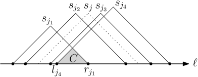
Figure 1: Illustrating the disks $s_{j_{1}}$, $s_{j_{2}}$, $s_{j_{3}}$, $s_{j_{4}}$, and $s_{j}$ for some $j\in[j_{2}+1,j_{3}-1]$; only the portions of the disks above $\ell$ are shown.

On the other hand, consider any $j\in[j_{2}+1,j_{3}-1]$. Since $j_{1}<j<j_{4}$, due to the Non-Containment property of $S$, $x(l_{j})\leq x(l_{j_{4}})$ and $x(r_{j_{1}})\leq x(r_{j})$, implying that $C\subseteq s_{j}$ since both $C$ and $s_{j}$ are diamonds (e.g., see Fig. 1). As $p_{i}\in C$, $p_{i}$ must hit $s_{j}$. But this incurs contradiction since $p_{i}$ does not hit $s_{j}$.

This proves that $|P_{i}^{*}|\leq 1$ for any $1\leq i\leq n$.

In the following, we describe an algorithm to compute $P_{i}^{*}$ for all $1\leq i\leq n$.

We sweep a vertical line $\ell^{\prime}$ in the plane from left to right. During the sweeping we maintain two subsets $S_{L}$ and $S_{R}$ of $S$: $S_{L}$ (resp., $S_{R}$) consists of all disks of $S$ whose upper left (resp., right) edges intersecting $\ell^{\prime}$; disks of $S_{L}$ (resp., $S_{R}$) are stored in a binary search tree $T_{L}$ (resp., $T_{R}$) sorted by the $y$-coordinates of the intersections between $\ell^{\prime}$ and the upper left (resp., right) edges of the disks of $S_{L}$ (resp., $S_{R}$). An event happens if $\ell^{\prime}$ encounters a point of $P$, the left endpoint, the right endpoint, or the center of a disk $s_{j}$.

If $\ell^{\prime}$ encounters the left endpoint of a disk $s_{j}$, we insert $s_{j}$ into $T_{L}$. If $\ell^{\prime}$ encounters the center of a disk $s_{j}$, we remove $s_{j}$ from $T_{L}$ and insert it into $T_{R}$. If $\ell^{\prime}$ encounters the right endpoint of a disk $s_{j}$, we remove $s_{j}$ from $T_{R}$. If $\ell^{\prime}$ encounters a point $p_{i}\in P$, we compute the only interval $[j_{1},j_{2}]$ of $P_{i}^{*}$ as follows.

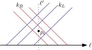
Figure 2: Illustrating the processing of the event at $p_{i}$: The red segments are the upper right edges of disks in $T_{R}$ and the blue segments are upper left edges of disks in $T_{L}$.

Using $T_{R}$, we find the disk of $T_{R}$ whose upper right edge is the lowest but above $p_{i}$; let $k_{R}$ be the index of the disk (e.g., see Fig. 2). Similarly, we find the disk of $T_{L}$ whose upper left edge is the lowest but above $p_{i}$; let $k_{L}$ be the index of the disk. Both $k_{R}$ and $k_{L}$ can be found in $O(\log m)$ time.

Assuming that both $k_{R}$ and $k_{L}$ are well defined, we claim that $j_{1}=k_{R}$ and $j_{2}=k_{L}$. Indeed, for any disk $s_{j}\in T_{R}$ that is below $s_{k_{R}}$, $p_{i}$ does not hit $s_{j}$ and $j<k_{R}$ due to the Non-Containment property of $S$. On the other hand, for any disk $s_{j}\in T_{R}$ that is above $s_{k_{R}}$, $p_{i}$ hits $s_{j}$ and $j>k_{R}$ due to the Non-Containment property of $S$. Similarly, for any disk $s_{j}\in T_{L}$ that is below $s_{k_{L}}$, $p_{i}$ does not hit $s_{j}$ and $j>k_{L}$, and for any disk $s_{j}\in T_{L}$ that is above $s_{k_{L}}$, $p_{i}$ hits $s_{j}$ and $j<k_{L}$. Note that the indices of disks in $T_{L}$ are larger than those in $S_{R}$ due to the Non-Containment property of $S$. Also note that disks not in $T_{L}$ or $T_{R}$ cannot be hit by $p_{i}$. As such, $j_{1}=k_{R}$ and $j_{2}=k_{L}$ must hold.

The above argument assumes that both $k_{R}$ and $k_{L}$ are well defined. If neither $k_{R}$ nor $k_{L}$ exists, then $P_{i}^{*}=\emptyset$. If $k_{R}$ exists while $k_{L}$ does not, then $j_{1}=k_{R}$ and $j_{2}$ is the index of the highest disk of $T_{R}$. If $k_{L}$ exists while $k_{R}$ does not, then $j_{2}=k_{L}$ and $j_{1}$ is the highest disk of $T_{L}$. The proof is similar to the above and we omit the details.

It is not difficult to see that the above sweeping algorithm can be implemented in $O((n+m)\log(n+m))$ time. ∎

In light of Lemma 3, using the dual transformation, the $L_{1}$ case can be solved in $O((n+m)\log(n+m))$ time.

Theorem 3.3

The line-constrained $L_{1}$ hitting set problem can be solved in $O((n+m)\log(n+m))$ time.

4 The $L_{\infty}$ metric

In this section, following the dual transformation, we present an $O((m+n)\log(m+n))$ time algorithm for $L_{\infty}$ case.

In the $L_{\infty}$ metric, each disk is a square whose edges are axis-parallel. For a disk $s_{j}\in S$ and a point $p_{i}\in P$, we say that $p$ is vertically above $s_{j}$ if $p_{i}$ is outside $s_{j}$ and $x(l_{j})\leq x(p_{i})\leq x(r_{j})$.

In the $L_{\infty}$ metric, using the dual transformation, it is easy to come up with an example in which $|P_{i}^{*}|\geq 2$. Observe that $|P_{i}^{*}|\leq\lceil m/2\rceil$ as the indices of $S$ can be partitioned into at most $\lceil m/2\rceil$ disjoint maximal intervals. Despite $|P_{i}^{*}|\geq 2$, the following critical lemma shows that each $P_{i}^{*}$ can contribute at most one segment to any optimal solution of the 1D dual coverage problem on $P^{*}$ and $S^{*}$.

Lemma 4

In the $L_{\infty}$ metric, for any optimal solution $P^{*}_{opt}$ of the 1D dual coverage problem on $P^{*}$ and $S^{*}$, $P^{*}_{opt}$ contains at most one segment from $P_{i}^{*}$ for any $1\leq i\leq n$.

Proof

Assume to the contrary that $P^{*}_{opt}$ contains more than one segment from $P_{i}^{*}$. Among all segments of $P^{*}_{opt}\cap P_{i}^{*}$, we choose two consecutive segments (recall that no two segments of $P_{i}^{*}$ are overlapped); we let $[j_{1},j_{2}]$ and $[j_{3},j_{4}]$ denote these two segments, respectively, with $j_{2}+1\leq j_{3}-1$ from $P_{i}^{*}$. Then all disks in $S[j_{1},j_{2}]\cup S[j_{3},j_{4}]$ are hit by $p_{i}$, while $s_{j}$ is not hit by $p_{i}$ for any $j\in[j_{2}+1,j_{3}-1]$.

We claim that $p_{i}$ is vertically above $s_{j}$ for any $j\in[j_{2}+1,j_{3}-1]$. To see this, since $j_{2}<j<j_{3}$, due to the Non-Containment property of $S$, $x(l_{j})\leq x(l_{j_{3}})$ and $x(r_{j})\geq x(r_{j_{2}})$. As $p_{i}$ hits both $s_{j_{2}}$ and $s_{j_{3}}$, we have $x(l_{j_{3}})\leq x(p_{i})\leq x(r_{j_{2}})$. As such, we obtain that $x(l_{j})\leq x(p_{i})\leq x(r_{j})$. Since $p_{i}$ does not hit $s_{j}$, $p_{i}$ must be vertically above $s_{j}$.

Let $\ell_{p_{i}}$ be the vertical line through $p_{i}$. The above claim implies that the upper edges of all disks of $S[j_{2}+1,j_{3}-1]$ intersect $\ell_{p_{i}}$. Among all disks of $S[j_{2}+1,j_{3}-1]$, let $s_{j_{0}}$ be the one whose upper edge is the lowest.

Since $P^{*}_{opt}$ is an optimal solution to the 1D dual coverage problem, one dual segment $[j_{5},j_{6}]\in P^{*}_{opt}$ defined by some point $p_{i^{\prime}}$ with $i\neq i^{\prime}$ must cover the dual point $s^{*}_{j_{0}}$, i.e., $p_{i^{\prime}}$ hits all disks $s_{j}$ with $j\in[j_{5},j_{6}]$ and $j_{0}\in[j_{5},j_{6}]$. In particular, $p_{i^{\prime}}$ hits $s_{j_{0}}$. In what follows, we prove that $[j_{5},j_{6}]$ must contain either $[j_{1},j_{2}]$ or $[j_{3},j_{4}]$. Depending on whether $x(p_{i}^{\prime})\leq x(p_{i})$, there are two cases.

• If $x(p_{i^{\prime}})\leq x(p_{i})$, we prove below that $p_{i^{\prime}}$ hits all disks $S[j_{1},j_{0}]$. Recall that $p_{i^{\prime}}$ hits $s_{j_{0}}$. Hence, it suffices to prove that $p_{i^{\prime}}$ hits $s_{j}$ for any $j\in[j_{1},j_{0}-1]$.

  Consider any $j\in[j_{1},j_{0}-1]$. We claim that the upper edge of $s_{j}$ must be higher than that of $s_{j_{0}}$. Indeed, if $j\in[j_{2}+1,j_{0}-1]$, then the claim is obviously true by the definition of $j_{0}$. Otherwise, $j\in[j_{1},j_{2}]$ and thus $p_{i}$ hits $s_{j}$. Hence, $p_{i}$ is lower than the upper edge of $s_{j}$. As $p_{i}$ is vertically above $s_{j_{0}}$, we obtain that the upper edge of $s_{j}$ must be higher than that of $s_{j_{0}}$. The claim thus follows.

  Since $j<j_{0}$, due to the Non-Containment property of $S$, we have $x(l_{j})\leq x(l_{j_{0}})$. Recall that $s_{j_{0}}$ intersects $\ell_{p_{i}}$. Since $p_{i}$ hits $s_{j}$, $s_{j}$ also intersects $\ell_{p_{i}}$. As such, since the upper edge of $s_{j}$ is higher than that of $s_{j_{0}}$, the portion of $s_{j_{0}}$ to the left of $\ell_{p_{i}}$ is a subset of the portion of $s_{j}$ to the left of $\ell_{p_{i}}$ (e.g., see Fig. 3). As $p_{i^{\prime}}$ hits $s_{j_{0}}$ and $x(p_{i^{\prime}})\leq x(p_{i})$, $p_{i^{\prime}}$ is inside the portion of $s_{j_{0}}$ to the left of $\ell_{p_{i}}$. Therefore, $p_{i^{\prime}}$ is inside the portion of $s_{j}$ to the left of $\ell_{p_{i}}$. Hence, $p_{i^{\prime}}$ hits $s_{j}$.

  

  Figure 3: Illustrating the proof of Lemma 4.

  This proves that $p_{i^{\prime}}$ hits all disks of $S[j_{1},j_{0}]$. As $j_{0}\in[j_{5},j_{6}]$, $[j_{1},j_{0}]$ must be contained in $[j_{5},j_{6}]$ since $[j_{5},j_{6}]$ is a maximal interval of indices of disks hit by $p_{i^{\prime}}$. Since $[j_{1},j_{2}]\subseteq[j_{1},j_{0}]$, we obtain that $[j_{5},j_{6}]$ must contain $[j_{1},j_{2}]$.

• If $x(p_{i^{\prime}})>x(p_{i})$, then by a symmetric analysis to the above, we can show that $[j_{5},j_{6}]$ must contain $[j_{3},j_{4}]$.

The above proves that $[j_{5},j_{6}]$ contains either $[j_{1},j_{2}]$ or $[j_{3},j_{4}]$. Without loss of generality, we assume that $[j_{5},j_{6}]$ contains $[j_{1},j_{2}]$. As $[j_{5},j_{6}]$ is in $P^{*}_{opt}$, if we remove $[j_{1},j_{2}]$ from $P^{*}_{opt}$, the rest of the intervals of $P^{*}_{opt}$ still form a coverage for all dual points of $S^{*}$, which contradicts with that $P^{*}_{opt}$ is an optimal coverage.

The lemma thus follows. ∎

The above lemma implies that an optimal solution to the 1D dual coverage problem on $P^{*}$ and $S^{*}$ still corresponds to an optimal solution of the original hitting set problem on $P$ and $S$. As such, it remains to compute the set $P^{*}$ of dual segments. In what follows, we first prove an upper bound for $|P^{*}|$.

4.1 Upper bound for $|P^{*}|$

As $|P^{*}_{i}|\leq\lceil m/2\rceil$, an obvious upper bound for $|P^{*}|$ is $O(mn)$. In the following, we reduce it to $O(m+n)$.

Our first observation is that if the same dual segment of $P^{*}$ is defined by more than one point of $P$, then we only need to keep the one whose weight is minimum. In this way, all segments of $P^{*}$ are distinct (i.e., $P^{*}$ is not a multi-set).

We sort all points of $P$ from top to bottom as $q_{1},q_{2},\ldots,q_{n}$. For ease of exposition, we assume that no point of $P$ has the same $y$-coordinate as the upper edge of any disk of $S$. For each $2\leq i\leq n$, let $S_{i}$ denote the subset of disks whose upper edges are between $q_{i-1}$ and $q_{i}$. Let $S_{1}$ denote the subset of disks whose upper edges are above $q_{1}$. For each $1\leq i\leq n$, let $m_{i}=|S_{i}|$.

We partition the indices of disks of $S_{1}$ into a set $\mathcal{I}_{1}$ of maximal intervals. Clearly, $|\mathcal{I}_{1}|\leq m_{1}$. The next lemma shows that other than the dual segments corresponding to the intervals in $\mathcal{I}_{1}$, $q_{1}$ can generate at most two dual segments in $P^{*}$.

Lemma 5

The number of dual segments of $P^{*}\setminus\mathcal{I}_{1}$ defined by $q_{1}$ is at most $2$.

Proof

Assume to the contrary that $q_{1}$ defines three intervals $[j_{1},j_{1}^{\prime}]$, $[j_{2},j_{2}^{\prime}]$, and $[j_{3},j_{3}^{\prime}]$ in $P^{*}\setminus\mathcal{I}_{1}$, with $j_{1}^{\prime}<j_{2}$ and $j_{2}^{\prime}<j_{3}$. By definition, $\mathcal{I}_{1}$ must have an interval, denoted by $I_{k}$, that strictly contains $[j_{k},j_{k}^{\prime}]$ (i.e., $[j_{k},j_{k}^{\prime}]\subset I_{k}$), for each $1\leq k\leq 3$. Then, $I_{2}$ must contain an index $j$ that is not in $[j_{1},j_{1}^{\prime}]\cup[j_{2},j_{2}^{\prime}]\cup[j_{3},j_{3}^{\prime}]$ with $j_{1}^{\prime}<j<j_{3}$ (e.g., see Fig. 4). As such, $q_{1}$ does not hit $s_{j}$. Also, since $j\in I_{2}$, $s_{j}$ is in $S_{1}$.

Figure 4: Illustrating a schematic view of the intervals $[j_{k},j_{k}^{\prime}]$ and $I_{k}$ for $1\leq k\leq 3$.

Since $j_{1}^{\prime}<j<j_{3}$, due to the Non-Containment property of $S$, $x(l_{j})\leq x(l_{j_{3}})$ and $x(r_{j_{1}^{\prime}})\leq x(r_{j})$. As $q_{1}$ hits both $s_{j_{1}^{\prime}}$ and $s_{j_{3}}$, we have $x(l_{j_{3}})\leq x(p_{1})\leq x(r_{j_{1}^{\prime}})$. Hence, we obtain $x(l_{j})\leq x(q_{1})\leq x(r_{j})$. Since $q_{1}$ does not hit $s_{j}$, the upper edge of $s_{j}$ must be below $q_{1}$. But this implies that $s_{j}$ is not in $S_{1}$, which incurs contradiction. ∎

Now we consider the disks of $S_{2}$ and the dual segments defined by $q_{2}$. For each disk $s_{j}$ of $S_{2}$, we update the intervals of $\mathcal{I}_{1}$ by adding the index $j$, as follows. Note that by definition, intervals of $\mathcal{I}_{1}$ are pairwise disjoint and no interval contains $j$.

1. If neither $j+1$ nor $j-1$ is in any interval of $\mathcal{I}_{1}$, then we add $[j,j]$ as a new interval to $\mathcal{I}_{1}$.

2. If $j+1$ is contained in an interval $I\in\mathcal{I}_{1}$ while $j-1$ is not, then $j+1$ must be the left endpoint of $I$. In this case, we add $j$ to $I$ to obtain a new interval $I^{\prime}$ (which has $j$ as its left endpoint) and add $I^{\prime}$ to $\mathcal{I}_{1}$; but we still keep $I$ in $\mathcal{I}_{1}$.

3. Symmetrically, if $j-1$ is contained in an interval $I\in\mathcal{I}_{1}$ while $j+1$ is not, then we add $j$ to $I$ to obtain a new interval $I^{\prime}$ and add $I^{\prime}$ to $\mathcal{I}_{1}$; we still keep $I$ in $\mathcal{I}_{1}$.

4. If both $j+1$ and $j-1$ are contained in intervals of $\mathcal{I}_{1}$, then they must be contained in two intervals, respectively; we merge these two intervals into a new interval by padding $j$ in between and adding the new interval to $\mathcal{I}_{1}$. We still keep the two original intervals in $\mathcal{I}_{1}$.

Let $\mathcal{I}_{1}^{\prime}$ denote the updated set $\mathcal{I}_{1}$ after the above operation. Clearly, $|\mathcal{I}_{1}^{\prime}|\leq|\mathcal{I}_{1}|+1$.

We process all disks $s_{j}\in S_{2}$ as above; let $\mathcal{I}_{2}$ be the resulting set of intervals. It holds that $|\mathcal{I}_{2}|\leq|\mathcal{I}_{1}|+|S_{2}|\leq m_{1}+m_{2}$. Also observe that for any interval $I$ of indices of disks of $S_{1}\cup S_{2}$ such that $I$ is not in $\mathcal{I}_{2}$, $\mathcal{I}_{2}$ must have an interval $I^{\prime}$ such that $I\subset I^{\prime}$ (i.e., $I\subseteq I^{\prime}$ but $I\neq I^{\prime}$). Using this property, by exactly the same analysis as Lemma 5, we can show that other than the intervals in $\mathcal{I}_{2}$, $q_{2}$ can generate at most two intervals in $P^{*}$. Since $\mathcal{I}_{1}\subseteq\mathcal{I}_{2}$, combining Lemma 5, we obtain that other than the intervals of $\mathcal{I}_{2}$, the number of intervals of $P^{*}$ generated by $q_{1}$ and $q_{2}$ is at most $4$.

We process disks of $S_{i}$ and point $q_{i}$ in the same way as above for all $i=3,4,\dots,n$. Following the same argument, we can show that for each $i$, we obtain an interval set $\mathcal{I}_{i}$ with $\mathcal{I}_{i-1}\subseteq\mathcal{I}_{i}$ and $|\mathcal{I}_{i}|\leq\sum_{k=1}^{i}m_{k}$, and other than the intervals of $\mathcal{I}_{i}$, the number of intervals of $P^{*}$ generated by $\{q_{1},q_{2},\ldots,q_{i}\}$ is at most $2i$. In particular, $|\mathcal{I}_{n}|\leq\sum_{k=1}^{n}m_{k}\leq m$, and other than the intervals of $\mathcal{I}_{n}$, the number of intervals of $P^{*}$ generated by $P=\{q_{1},q_{2},\ldots,q_{n}\}$ is at most $2n$. We thus achieve the following conclusion.

Lemma 6

In the $L_{\infty}$ metric, $|P^{*}|\leq 2n+m$.

4.2 Computing $P^{*}$

Using Lemma 6, we next present an algorithm that computes $P^{*}$ in $O((n+m)\log(n+m))$ time.

For each segment $I\in P^{*}$, let $w(I)$ denote its weight. We say that a segment $I$ of $P^{*}$ is redundant if there is another segment $I^{\prime}$ such that $I\subset I^{\prime}$ and $w(I)\geq w(I^{\prime})$. Clearly, any redundant segment of $P^{*}$ cannot be used in any optimal solution for the 1D dual coverage problem on $S^{*}$ and $P^{*}$. A segment of $P^{*}$ is non-redundant if it is not redundant.

In the following algorithm, we will compute a subset $P^{*}_{0}$ of $P^{*}$ such that segments of $P^{*}\setminus P^{*}_{0}$ are all redundant (i.e., the segments of $P^{*}$ that are not computed by the algorithm are all redundant and thus are useless). We will show that each segment reported by the algorithm belongs to $P^{*}$ and thus the total number of reported segments is at most $2n+m$ by Lemma 6. We will show that the algorithm spends $O(\log(n+m))$ time reporting one segment and each segment is reported only once; this guarantees the $O((n+m)\log(n+m))$ upper bound of the runtime of the algorithm.

For each disk $s_{j}\in S$, we use $y(s_{j})$ to denote the $y$-coordinate of the upper edge of $s_{j}$.

Our algorithm has $m$ iterations. In the $j$-th iteration, it computes all segments in $P^{*}_{j}$, where $P^{*}_{j}$ is the set of all non-redundant segments of $P^{*}$ whose starting indices are $j$, although it is possible that some redundant segments with starting index $j$ may also be computed. Points of $P$ defining these segments must be inside $s_{j}$; let $P_{j}$ denote the set of points of $P$ inside $s_{j}$. We partition $P_{j}$ into two subsets (e.g., see Fig. 5): $P_{j}^{1}$ consists of points of $P_{j}$ to the left of $r_{j-1}$ and $P_{j}^{2}$ consists of points of $P_{j}$ to the right of $r_{j-1}$. We will compute dual segments of $P^{*}_{j}$ defined by $P_{j}^{1}$ and $P_{j}^{2}$ separately; one reason for doing so is that when computing dual segments defined by a point of $P_{j}^{1}$, we need to additionally check whether this point also hits $s_{j-1}$ (if yes, such a dual segment does not exist in $P^{*}$ and thus will not be reported). In the following, we first describe the algorithm for $P_{j}^{1}$ since the algorithm for $P_{j}^{2}$ is basically the same but simpler. Note that our algorithm does not need to explicitly determine the points of $P_{j}^{1}$ or $P_{j}^{2}$; rather we will build some data structures that can implicitly determine them during certain queries.

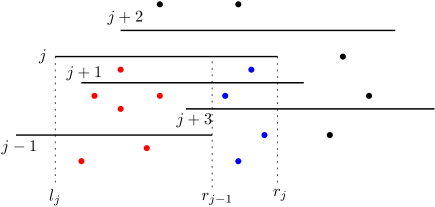
Figure 5: Illustrating $P_{j}^{1}$ (the red points) and $P_{j}^{2}$ (the blue points). Only the upper edges of disks are shown. The numbers are the indices of disks.

If the upper edge of $s_{j-1}$ is higher than that of $s_{j}$, then all points of $P_{j}^{1}$ are in $s_{j-1}$ and thus no point of $P_{j}^{1}$ defines any dual segment of $P^{*}$ starting from $j$. Indeed, assume to the contrary that a point $p_{i}\in P_{j}^{1}$ defines such a dual segment $[j,j^{\prime}]$. Then, since $p_{i}$ is in $s_{j-1}$, $[j,j^{\prime}]$ cannot be a maximal interval of indices of disks hit by $p_{i}$ and thus cannot be a dual segment defined by $p_{i}$. In what follows, we assume that the upper edge of $s_{j-1}$ is lower than that of $s_{j}$. In this case, it suffices to only consider points of $P_{j}^{1}$ above $s_{j-1}$ since points below the upper edge of $s_{j-1}$ (and thus are inside $s_{j-1}$) cannot define any dual segments due to the same reason as above. Nevertheless, our algorithm does not need to explicitly determine these points.

We start with performing the following rightward segment dragging query: Drag the vertical segment $x(l_{j})\times[y(s_{j-1}),y(s_{j})]$ rightwards until a point $p\in P$ and return $p$ (e.g., see Fig. 6). Such a segment dragging query can be answered in $O(\log n)$ time after $O(n\log n)$ time preprocessing on $P$ (e.g., using Chazelle’s result [6] one can build a data structure of $O(n)$ space in $O(n\log n)$ time such that each query can be answered in $O(\log n)$ time; alternatively, if one is satisfied with an $O(n\log n)$ space data structure, then an easier solution is to use fractional cascading [8] and one can build a data structure in $O(n\log n)$ time and space with $O(\log n)$ query time). If the query does not return any point or if the query returns a point $p$ with $x(p)>x(r_{j-1})$, then $P_{j}^{1}$ does not have any point above $s_{j-1}$ and we are done with the algorithm for $P_{j}^{1}$. Otherwise, suppose the query returns a point $p$ with $x(p)\leq x(r_{j-1})$; we proceed as follows.

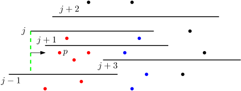
Figure 6: Illustrating the rightward segment dragging query: the green dashed segment is the dragged segment $x(l_{j})\times[y(s_{j-1}),y(s_{j})]$.

We perform the following max-range query on $p$: Compute the largest index $k$ such that all disks in $S[j,k]$ are hit by $p$ (e.g., in Fig. 6, $k=j+2$). We will show later in Lemma 7 that after $O(m\log m)$ time and $O(m)$ space processing, each such query can be answered in $O(\log m)$ time. Such an index $k$ must exist as $s_{j}$ is hit by $p$. Observe that $[j,k]$ is a dual segment in $P^{*}$ defined by $p$. However, the weight of $[j,k]$ may not be equal to $w(p)$, because it is possible that a point with smaller weight also defines $[j,k]$. Our next step is to determine the minimum-weight point that defines $[j,k]$.

We perform a range-minima query on $[j,k]$: Find the lowest disk among all disks in $S[j,k]$ (e.g., in Fig. 6, $s_{j+1}$ is the answer to the query). This can be easily done in $O(\log m)$ time with $O(m)$ space and $O(m\log m)$ time preprocessing. Indeed, we can build a binary search tree on the upper edges of all disks of $S$ with their $y$-coordinates as keys and have each node storing the lowest disk among all leaves in the subtree rooted at the node. A better but more complicated solution is to build a range-minima data structure on the $y$-coordinates of the upper edges of all disks in $O(m)$ time and each query can be answered in $O(1)$ time [2, 17]. However, the above binary search tree solution is sufficient for our purpose. Let $y^{*}$ be the $y$-coordinate of the upper edge of the disk returned by the query.

We next perform the following downward min-weight point query for the horizontal segment $[x(l_{k}),x(r_{j-1})]\times y^{*}$: Find the minimum weight point of $P$ below the segment (e.g., see Fig. 7). We will show later in Lemma 8 that after $O(n\log n)$ time and space preprocessing, each query can be answered in $O(\log n)$ time. Let $p^{\prime}$ be the point returned by the query. If $p^{\prime}=p$, then we report $[j,k]$ as a dual segment with weight equal to $w(p)$. Otherwise, if $p^{\prime}$ is inside $s_{j-1}$ or $s_{k+1}$, then $[j,k]$ is a redundant dual segment (because a dual segment defined by $p^{\prime}$ strictly contains $[j,k]$ and $w(p^{\prime})\leq w(p)$) and thus we do not need to report it. In any case, we proceed as follows.

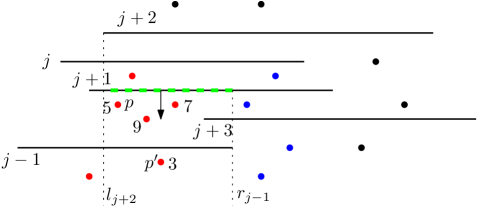
Figure 7: Illustrating the downward min-weight point query (with $k=j+2$): the green dashed segment is the dragged segment $[x(l_{k}),x(r_{j-1})]\times y^{*}$. The numbers besides the points are their weights. The answer to the query is $p^{\prime}$, whose weight is $3$.

The above basically determines that $[j,k]$ is a dual segment in $P^{*}$. Next, we proceed to determine those dual segments $[j,k^{\prime}]$ with $k^{\prime}>k$. If such a dual segment exists, the interval $[j,k^{\prime}]$ must contain index $k+1$. Hence, we next consider $s_{k+1}$. If $y(s_{k+1})>y(s_{j-1})$, then let $y^{\prime}=\min\{y^{*},y(s_{k+1})\}$; we perform a rightward segment dragging query with the vertical segment $x(l_{k+1})\times[y(s_{j-1}),y^{\prime}]$ (e.g., see Fig. 8) and then repeat the above algorithm. If $y(s_{k+1})\leq y(s_{j-1})$, then points of $P_{j}^{1}$ above $s_{j-1}$ are also above $s_{k+1}$ and thus no point of $P_{j}^{1}$ can generate any dual segment $[j,k^{\prime}]$ with $k^{\prime}>k$ and thus we are done with the algorithm on $P_{j}^{1}$.

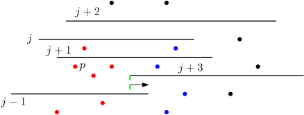
Figure 8: Illustrating the rightwards segment dragging query: the green dashed segment is the dragged segment $x(l_{k+1})\times[y(s_{j-1}),y^{\prime}]$.

For the time analysis, we charge the time of the above five queries to the interval $[j,k]$, which is in $P^{*}$. Note that $[j,k]$ will not be charged again in the future because future queries in the $j$-th iteration will be charged to $[j,k^{\prime}]$ for some $k^{\prime}>k$ and future queries in the $j^{\prime}$-th iteration for any $j^{\prime}>j$ will be charged to $[j^{\prime},k^{\prime\prime}]$. As such, each dual segment of $P^{*}$ will be charged $O(1)$ times during the entire algorithm. As each query takes $O(\log(n+m))$ time, the total time of all queries in the entire algorithm is $O(|P^{*}|\log(n+m))$, which is $((n+m)\log(n+m))$ by Lemma 6.

Lemma 7

With $O(m\log m)$ time and $O(m)$ space preprocessing on $S$, each max-range query can be answered in $O(\log m)$ time.

Proof

We build a complete binary search tree $T$ with $m$ leaves storing the disks of $S$ in their index order. For each node $v\in T$, we store a value $y_{v}$ that is equal to the minimum $y(s_{j})$ for all disks $s_{j}$ stored in the leaves of the subtree rooted at $v$. In addition, we use an array $A$ to store all disks sorted by their indices. This finishes our preprocessing, which takes $O(m\log m)$ time and $O(m)$ space.

Given a query point $p$ and a disk index $j$ with $p$ hitting $s_{j}$, the max-range query asks for the largest index $k$ such that all disks of $S[j,k]$ are hit by $p$. Our query algorithm has two main steps. In the first step, we use the tree $T$ to find in $O(\log m)$ time the largest index $k^{\prime}$ such that $y(s_{t})\geq y(p)$ for all $t\in[j,k^{\prime}]$; the details of the algorithm will be described later. In the second step, using the array $A$, we find the largest index $k^{\prime\prime}$ such that $x(l_{k^{\prime\prime}})\leq x(p)$. As the disks in $A$ are sorted by their indices, due to the Non-Containment property, the disks $s_{j}$ of $A$ are also sorted by the values $x(l_{j})$. Hence, $k^{\prime\prime}$ can be found in $O(\log m)$ time by binary search on $A$. As $p$ hits $s_{j}$, we have $x(l_{j})\leq x(p)$ and thus $j\leq k^{\prime\prime}$. After having $k^{\prime}$ and $k^{\prime\prime}$, we return $k=\{k^{\prime},k^{\prime\prime}\}$ as the answer to the max-range query. In the following, we prove the correctness: $k$ thus defined is the largest index such that all disks of $S[j,k]$ are hit by $p$. Depending on whether $k^{\prime}\leq k^{\prime\prime}$, there are two cases.

1. If $k^{\prime}\leq k^{\prime\prime}$, then $k=k^{\prime}$. By the definition of $k^{\prime}$, $y(s_{k^{\prime}+1})<y(p)$ and thus $p$ does not hit $s_{k^{\prime}+1}$. Hence, if suffices to prove that $p$ hits $s_{t}$ for all $t\in[j,k^{\prime}]$. Indeed, since $t\leq k^{\prime}\leq k^{\prime\prime}$, by the definition of $k^{\prime\prime}$, we have $x(l_{t})\leq x(p)$. On the other hand, since $p$ hits $s_{j}$, we have $x(p)\leq x(r_{j})$. Since $j\leq t$, by the Non-Containment property of $S$, $x(r_{j})\leq x(r_{t})$. Therefore, we obtain $x(p)\leq x(r_{t})$. Finally, as $t\leq k^{\prime}$, by the definition of $k^{\prime}$, $y(p)\leq y(s_{t})$.

   In summary, we have $x(l_{t})\leq x(p)\leq x(r_{t})$ and $y(p)\leq y(s_{t})$. Therefore, $p$ hits $s_{t}$. This proves that $k=k^{\prime}$ is the largest index such that all disks of $S[j,k]$ are hit by $p$.

2. If $k^{\prime}>k^{\prime\prime}$, then $k=k^{\prime\prime}$. By the definition of $k^{\prime\prime}$, $x(l_{k^{\prime\prime}+1})>x(p)$ and thus $p$ does not hit $s_{k^{\prime\prime}+1}$. Hence, if suffices to prove that $p$ hits $s_{t}$ for all $t\in[j,k^{\prime\prime}]$. Indeed, since $t\leq k^{\prime\prime}$, by the definition of $k^{\prime\prime}$, we have $x(l_{t})\leq x(p)$. On the other hand, since $p$ hits $s_{j}$, we have $x(p)\leq x(r_{j})$. Since $j\leq t$, by the Non-Containment property of $S$, $x(r_{j})\leq x(r_{t})$. Therefore, we obtain $x(p)\leq x(r_{t})$. Finally, as $t\leq k^{\prime\prime}<k^{\prime}$, by the definition of $k^{\prime}$, $y(p)\leq y(s_{t})$.

   In summary, we have $x(l_{t})\leq x(p)\leq x(r_{t})$ and $y(p)\leq y(s_{t})$. Therefore, $p$ hits $s_{t}$. This proves that $k=k^{\prime\prime}$ is the largest index such that all disks of $S[j,k]$ are hit by $p$.

It remains to describe the algorithm for computing $k^{\prime}$ using $T$. The algorithm has two phases. Starting from the leaf storing disk $s_{j}$, for each node $v$, we process it as follows. Let $u$ be the parent of $v$. If $v$ is the right child of $u$, then we proceed on $u$ recursively by setting $v=u$. If $v$ is the left child of $u$, then let $w$ be the right child of $u$. If $y_{w}\geq y(p)$, then we proceed on $u$ recursively by setting $v=u$. Otherwise, the first phase of the algorithm is over and the second phase starts from $v=w$ in a top-down manner as follows. Let $u$ and $w$ be the left and right children of $v$ recursively. If $y_{u}\geq y(p)$, then we proceed on $w$ recursively by setting $v=w$; otherwise we proceed on $u$ recursively by setting $v=u$. When we reach a leaf $v$, which stores a disk $s_{t}$, if $y(s_{t})\geq y(p)$, then we return $k^{\prime}=t$; otherwise we return $k^{\prime}=t-1$. Clearly, the algorithm runs in $O(\log m)$ time.

The lemma thus follows. ∎

Lemma 8

With $O(n\log n)$ time and space preprocessing on $P$, each downward min-weight point query can be answered in $O(\log n)$ time.

Proof

Recall that the downward min-weight point query is to compute the minimum weight point of $P$ below a query horizontal segment.

We built a complete binary search tree $T$ whose leaves store points of $P$ from left to right. For each node $v\in T$, let $P_{v}$ denote the subset of points of $P$ in the leaves of the subtree rooted at $v$. We compute a subset $P_{v}^{\prime}\subseteq P_{v}$ with the following property: (1) If we sort all points of $P_{v}^{\prime}$ in the order of decreasing $y$-coordinate, then the weights of the points are sorted in increasing order; (2) for any point $p\in P_{v}\setminus P_{v}^{\prime}$, $P_{v}^{\prime}$ must have a point $p^{\prime}$ below $p$ with $w(p^{\prime})\leq w(p)$. We compute $P_{v}^{\prime}$ for all $v\in T$ in a bottom-up manner as follows. Initially, let $P_{v}^{\prime}=P_{v}$ for all leaves $v\in T$. Consider an internal node $v$. We assume that both $P_{u}^{\prime}$ and $P_{w}^{\prime}$ are computed already, where $u$ and $w$ are the two children of $v$. We also assume that points of both $P_{u}^{\prime}$ and $P_{w}^{\prime}$ are sorted by $y$-coordinate. The subset $P_{v}^{\prime}$ is computed by merging $P_{u}^{\prime}$ and $P_{w}^{\prime}$ as follows.

We scan the two sorted lists of $P_{u}^{\prime}$ and $P_{w}^{\prime}$ in decreasing $y$-coordinate order, in the same way as merge sort. Suppose we are comparing two points $p_{u}\in P_{u}^{\prime}$ and $p_{w}\in P_{w}^{\prime}$ and the higher one will be placed at the end of an already sorted list $L$ (assume that the lowest point of $L$ is higher than both $p_{u}$ and $p_{w}$; initially $L=\emptyset$). Suppose $p_{u}$ is higher than $p_{w}$. In the normal merge sort, one would just place $p_{u}$ at the end of $L$. Here we do the following. Let $p$ be the lowest point of $L$. If $w(p_{u})>w(p)$, then add $p_{u}$ to the end of $L$. Otherwise, we remove $p$ from $L$ (we say that $p$ is pruned), and then we keep pruning the next lowest point of $L$ until its weight is smaller than $w(p_{u})$ and finally we place $p_{u}$ at the end of $L$. Clearly, the time for computing $P_{v}^{\prime}$ is bounded by $O(|P_{u}^{\prime}|+|P_{w}^{\prime}|)$.

In this way, we can compute $P_{v}^{\prime}$ for all nodes $v\in T$ in $O(n\log n)$ time and space. Next, we construct a fractional cascading data structure [8] on the sorted lists of $P_{v}^{\prime}$ of all nodes $v\in T$, which can be done in time linear to the total size of all lists, which is $O(n\log n)$. This finishes the preprocessing, which takes $O(n\log n)$ time and space.

Given a query horizontal segment $B=[x_{1},x_{2}]\times y$, our goal is to find the minimum weight point among all points of $P$ below $B$. Using the standard approach, we can find in $O(\log n)$ time a set $V$ of $O(\log n)$ nodes such that the union $\bigcup_{v\in V}P_{v}$ is exactly the subset of points of $P$ whose $x$-coordinates are in $[x_{1},x_{2}]$ and parents of nodes of $V$ are on two paths of $T$ from the root to two nodes. For each node $v\in V$, we wish to find the highest point $p_{v}$ of $P_{v}^{\prime}$ below $B$. Due to the above Property (2) of $P_{v}^{\prime}$, $p_{v}$ must be the minimum weight point below $B$ among all points of $P_{v}$. We can compute $p_{v}$ for all $v\in V$ in $O(\log n)$ time using the fractional cascading data structure [8], after which we return the highest $p_{v}$ among all $v\in V$ as the answer to the query. The total time of the query algorithm is $O(\log n)$.

This proves the lemma. ∎

This finishes the description of the algorithm for $P_{j}^{1}$. The algorithm for $P_{j}^{2}$ is similar with the following minor changes. First, when doing each rightward segment dragging query, the lower endpoint of the query vertical segment is at $-\infty$ instead of $y(s_{j-1})$. Second, when the downward min-weight point query returns a point, we do not have to check whether it is in $s_{j-1}$ anymore. The rest of the algorithm is the same. In this way, all non-redundant intervals of $P^{*}$ starting at index $j$ can be computed. As analyzed above, the runtime of the entire algorithm is bounded by $O((n+m)\log(n+m))$.

As such, using the dual transformation, the $L_{\infty}$ case can be solved in $O((n+m)\log(n+m))$ time.

Theorem 4.1

The line-constrained $L_{\infty}$ hitting set problem can be solved in $O((n+m)\log(n+m))$ time.

5 The $L_{2}$ case

In this section, following the dual transformation, we solve $L_{2}$ hitting set problem.

Recall that we have made a general position assumption that no point of $P$ is on the boundary of a disk of $S$. In the $L_{2}$ metric, $l_{j}$ (resp., $r_{j}$) is the only leftmost (resp., rightmost) point of disk $s_{j}$. For a disk $s_{j}\in S$ and a point $p_{i}\in P$, we say that $p_{i}$ is vertically above $s_{j}$ if $p_{i}$ is outside $s_{j}$ and $x(l_{j})\leq x(p_{i})\leq x(r_{j})$. For any disk $s_{j}$, we use $\partial s_{j}$ to denote the portion of its boundary above $\ell$, which is a half-circle. Note that $\partial s_{j}$ and $\partial s_{k}$ have at most one intersection, for any two disks $s_{j}$ and $s_{k}$.

As in the $L_{\infty}$ case, it is possible that $|P_{i}^{*}|\geq 2$; $|P_{i}^{*}|\leq\lceil m/2\rceil$ also holds. We have the following lemma, whose proof follows the scheme of Lemma 4 although the details are not exactly the same.

Lemma 9

In the $L_{2}$ metric, for any optimal solution $P^{*}_{opt}$ to the 1D dual coverage problem on $P^{*}$ and $S^{*}$, $P^{*}_{opt}$ contains at most one dual segment from $P_{i}^{*}$ for any $1\leq i\leq n$.

Proof

Assume to the contrary that $P^{*}_{opt}$ contains more than one segment from $P_{i}^{*}$. Among all segments of $P^{*}_{opt}\cap P_{i}^{*}$, we choose two consecutive segments $[j_{1},j_{2}]$ and $[j_{3},j_{4}]$; thus $j_{2}+1\leq j_{3}-1$. Then all disks in $S[j_{1},j_{2}]\cup S[j_{3},j_{4}]$ are hit by $p_{i}$, while $s_{j}$ is not hit by $p_{i}$ for any $j\in[j_{2}+1,j_{3}-1]$.

Due to the Non-Containment property of $S$, following the argument in Lemma 4, $p_{i}$ is vertically above $s_{j}$ for any $j\in[j_{2}+1,j_{3}-1]$. Among all disks of $S[j_{2}+1,j_{3}-1]$, let $s_{j_{0}}$ be the one whose boundary has the lowest intersection with $\ell_{p_{i}}$, where $\ell_{p_{i}}$ is the vertical line through $p_{i}$.

Since $P^{*}_{opt}$ is an optimal solution, a dual segment $[j_{5},j_{6}]\in P^{*}$ defined by some point $p_{i^{\prime}}$ with $i\neq i^{\prime}$ must cover the dual point $s^{*}_{j_{0}}$, i.e., $p_{i^{\prime}}$ hits all disks $s_{j}$ with $j\in[j_{5},j_{6}]$ and $j_{0}\in[j_{5},j_{6}]$. In particular, $p_{i^{\prime}}$ hits $s_{j_{0}}$. In what follows, we prove that $[j_{5},j_{6}]$ must contain either $[j_{1},j_{2}]$ or $[j_{3},j_{4}]$. Depending on whether $x(p_{i^{\prime}})\leq x(p_{i})$, there are two cases.

Figure 9: Illustrating the proof of Lemma 9.

• If $x(p_{i^{\prime}})\leq x(p_{i})$, we prove below that $p_{i^{\prime}}$ hits all disks $S[j_{1},j_{0}]$. Recall that $p_{i^{\prime}}$ hits $s_{j_{0}}$. Hence, it suffices to prove that $p_{i^{\prime}}$ hits $s_{j}$ for any $j\in[j_{1},j_{0}-1]$. Consider any $j\in[j_{1},j_{0}-1]$.

  We claim that the intersection of $\partial s_{j}$ with $\ell_{p_{i}}$ must be higher than that of $\partial s_{j_{0}}$. Indeed, if $j\in[j_{2}+1,j_{0}-1]$, then this follows the definition of $j_{0}$. If $j\leq j_{2}$, then $p_{i}$ must hit $s_{j}$. Hence, $p_{i}$ is below $\partial s_{j}$. Because $p_{i}$ is vertically above $s_{j_{0}}$, the claim follows.

  Since $j<j_{0}$, due to the Non-Containment property, $x(l_{j})<x(l_{j_{0}})$. Since $\partial s_{j}$ and $\partial s_{j_{0}}$ cross each other at most once, the above claim implies that $s_{j}$ and $s_{j_{0}}$ do not cross each other on the left side of $\ell_{p_{i}}$ (e.g., see Fig. 9). As $p_{i^{\prime}}$ is to the left of $\ell_{p_{i}}$ and $p_{i^{\prime}}$ is inside $s_{j_{0}}$, the above further implies that $p_{i^{\prime}}$ is inside $s_{j}$ as well (e.g., see Fig. 9).

  This proves that $p_{i^{\prime}}$ hits all disks of $S[j_{1},j_{0}]$. As $j_{0}\in[j_{5},j_{6}]$, $[j_{1},j_{0}]$ must be contained in $[j_{5},j_{6}]$ since $[j_{5},j_{6}]$ is a maximal interval of indices of disks hit by $p_{i^{\prime}}$. Since $[j_{1},j_{2}]\subseteq[j_{1},j_{0}]$, we obtain that $[j_{5},j_{6}]$ must contain $[j_{1},j_{2}]$.

• If $x(p_{i^{\prime}})>x(p_{i})$, then by a symmetric analysis to the above, we can show that $[j_{5},j_{6}]$ must contain $[j_{3},j_{4}]$.

The above proves that $[j_{5},j_{6}]$ contains either $[j_{1},j_{2}]$ or $[j_{3},j_{4}]$. Without loss of generality, we assume that $[j_{5},j_{6}]$ contains $[j_{1},j_{2}]$. As $[j_{5},j_{6}]$ is in $P^{*}_{opt}$, if we remove $[j_{1},j_{2}]$ from $P^{*}_{opt}$, the rest of the intervals of $P^{*}_{opt}$ still form a coverage for all dual points of $S^{*}$, which contradicts with that $P^{*}_{opt}$ is an optimal coverage.

The lemma thus follows. ∎

As in the $L_{\infty}$ case, the above lemma implies that it suffices to find an optimal solution to the 1D dual coverage problem on $P^{*}$ and $S^{*}$.

5.1 Upper bound for $|P^{*}|$

As $|P_{i}^{*}|\leq\lceil m/2\rceil$, an obvious upper bound for $|P^{*}|$ is $O(mn)$. In this section, with some observations, we show that $|P^{*}|=O(m+\kappa)$, where $\kappa$ is the number of pairs of disks of $S$ that intersect.

Let $H$ denote the upper half-plane bounded by $\ell$. Consider two disks $s_{j}$ and $s_{k}$ whose boundaries intersect, say, at a point $v$. The boundaries of $s_{j}$ and $s_{j^{\prime}}$ partition $H$ into four regions. One region is inside both disks; another region is outside both disks. Each of the remaining two regions is contained in exactly one of the disks; we call them the wedges of $v$ (resp., $s_{j}$ and $s_{j^{\prime}}$). One wedge has $v$ as its rightmost point and we call it the left wedge; the other wedge has $v$ as its leftmost point and we call it the right wedge (e.g., see Fig. 10).

Figure 10: Illustrating left and right wedges of two disks that intersect.

Let $\mathcal{A}$ be the arrangement of the boundaries of all disks of $S$ in the half-plane $H$. $\mathcal{A}$ has a single face that is outside all disks; for convenience, we remove it from $\mathcal{A}$. Observe that points of $P$ located in the same face of $\mathcal{A}$ define the same subset of dual segments of $P^{*}$. Hence it suffices to consider the dual segments defined by all faces of $\mathcal{A}$.

Due to that all disks of $S$ are centered on $\ell$ as well as the Non-Containment property of $S$, we discuss some properties of the faces of $\mathcal{A}$. For convenience, we consider $\ell$ as the boundary of a disk with an infinite radius and with its center below $\ell$ (thus $H$ is the region outside the disk); let $s^{\prime}$ denote the disk and let $S^{\prime}=S\cup\{s^{\prime}\}$. Consider a face $f\in\mathcal{A}$. Each edge $e$ of $f$ is a circular arc on the boundary of a disk $s_{e}$ of $S^{\prime}$, such that $f$ is either inside or outside the disk $s_{e}$. More specifically, if $u$ and $v$ are leftmost and rightmost vertices of $f$, respectively, then $u$ and $v$ partition the boundary of $f$ into an upper chain and a lower chain (both chains are $x$-monotone). For each edge $e$ in the upper (resp., lower) chain, $f$ is inside (resp., outside) $s_{e}$. As the boundaries of every two disks of $S$ cross each other at most once, the boundary of each disk contributes at most one edge of $f$. Consider the leftmost vertex $u$ of $f$, which is incident two edges of $f$, one edge $e_{a}$ on the upper chain and the other edge $e_{b}$ on the lower chain. If $e_{b}$ is on $\ell$, then $u$ is actually the leftmost point of the disk whose boundary contains $e_{a}$; in this case, we call $f$ an initial face (e.g., see Fig. 11). If $f$ is not an initial face, we say that $f$ is a non-initial face; in this case, $u$ must be the rightmost vertex of another face $f^{\prime}$ such that $f^{\prime}$ is in the left wedge of $u$ while $f$ is in the right wedge of $u$, and we call $f^{\prime}$ the opposite face of $f$ (e.g., see Fig. 12).

Figure 11: Illustrating an initial face $f$ with leftmost vertex $u$.

Figure 12: Illustrating a non-initial face $f$ with leftmost vertex $u$ and its opposite face $f^{\prime}$.

To help the analysis, we introduce a directed graph $G$, defined as follows. The faces of $\mathcal{A}$ form the node set of $G$. There is an edge from a node $f^{\prime}$ to another node $f$ if the face $f$ is a non-initial face and $f^{\prime}$ is the opposite face of $f$ (i.e., the rightmost vertex of $f^{\prime}$ is the leftmost vertex of $f$; e.g., in Fig. 12, there is a directed edge from $f^{\prime}$ to $f$). Since each face of $\mathcal{A}$ has only one leftmost vertex and only one rightmost vertex, each node $G$ has at most one incoming edge and at most one outgoing edge. Observe that each initial face does not have an incoming edge while each non-initial face must have an incoming edge. As such, $G$ is actually composed of a set of paths, each of which has an initial face as the first node.

For each face $f\in\mathcal{A}$, we use $P^{*}(f)$ to denote the subset of the dual segments of $P^{*}$ generated by $f$ (i.e, generated by any point in $f$). Our goal is to obtain an upper bound for $|\bigcup_{f\in\mathcal{A}}P^{*}(f)|$, which will be an upper bound for $|P^{*}|$ as $P^{*}\subseteq\bigcup_{f\in\mathcal{A}}P^{*}(f)$. The following lemma proves that each initial face can only generate one dual segment.

Lemma 10

For each initial face $f$, $|P^{*}(f)|=1$.

Proof

Let $u$ be the leftmost vertex of $f$. By the definition of initial faces, $u$ is the leftmost point $l_{k}$ of a disk $s_{k}$ and $f\subseteq s_{k}$. In the following, we show that indices of all disks of $S$ containing $l_{k}$ must form an interval $[k^{\prime},k]$ for some $k^{\prime}\leq k$, which will prove the lemma.

Indeed, for any disk $s_{j}$ with $j>k$, due to the Non-Containment property of $S$, $x(l_{k})<x(l_{j})$ and thus $s_{j}$ cannot contain $l_{k}$. On the other hand, suppose $s_{j}$ contains $l_{k}$ for some $j<k$. Then, for any $j^{\prime}$ with $j<j^{\prime}<k$, we claim that $s_{j^{\prime}}$ contains $l_{k}$. It suffices to show that $x(l_{j^{\prime}})<x(l_{k})<x(r_{j^{\prime}})$. Due to the Non-Containment property of $S$, we have $x(l_{j^{\prime}})<x(l_{k})$. Also, since $s_{j}$ contains $l_{k}$, we have $x(l_{j})<x(l_{k})<x(r_{j})$. Due to the Non-Containment property, since $j<j^{\prime}$, we have $x(r_{j})<x(r_{j^{\prime}})$. As such, we obtain $x(l_{k})<x(r_{j^{\prime}})$. The claim thus follows, which leads to the lemma. ∎

The next lemma shows that for any two adjacent faces $f^{\prime}$ and $f$ in any path of $G$, the symmetric difference between $P^{*}(f^{\prime})$ and $P^{*}(f)$ is of constant size.

Lemma 11

For any two adjacent faces $f^{\prime}$ and $f$ in any path of $G$, $|P^{*}(f)\setminus P^{*}(f^{\prime})|\leq 3$ and $|P^{*}(f^{\prime})\setminus P^{*}(f)|\leq 3$.

Proof

As $f^{\prime}$ and $f$ are adjacent in a path of $G$, without loss of generality, we assume that there is a directed edge from $f^{\prime}$ to $f$. By definition, $f^{\prime}$ and $f$ share a vertex $u$ that is the rightmost vertex of $f^{\prime}$ and also the leftmost vertex of $f$ (e.g., see Fig. 13).

Figure 13: Illustrating two faces $f^{\prime}$ and $f$ that are adjacent in a path of $G$. The vertex $u$, which is the intersection of the boundaries of two disks $s$ and $s^{\prime}$, is the rightmost vertex of $f^{\prime}$ and also the leftmost vertex of $f$.

We define $S(f)$ as the subset of disks of $S$ containing $f$ and define $S(f^{\prime})$ similarly. By definition, $P^{*}(f)$ (resp., $P^{*}(f^{\prime})$) is the set of maximal intervals of indices of disks of $S(f)$ (resp., $S(f^{\prime})$). It is easy to see that the symmetric difference of $S(f)$ and $S(f^{\prime})$ comprises exactly two disks, i.e., the two disks whose boundaries intersect at $u$. As such, a straightforward analysis can prove that $|P^{*}(f)\setminus P^{*}(f^{\prime})|\leq 3$ and $|P^{*}(f^{\prime})\setminus P^{*}(f)|\leq 3$ as follows. Indeed, let $s$ be the disk of $S(f^{\prime})\setminus S(f)$ and $s^{\prime}$ be the disk of $S(f)\setminus S(f^{\prime})$. Hence, $s$ contains $f^{\prime}$ but not $f$ while $s^{\prime}$ contains $f$ but not $f^{\prime}$ (e.g., see Fig. 13). As such, comparing $P^{*}(f)$ to $P^{*}(f^{\prime})$, we have the following two cases.

• Due to that $S(f)$ “loses” a disk (i.e., $s$) comparing to $S(f^{\prime})$, at most two new dual segments are generated in $P^{*}(f)$ comparing to $P^{*}(f^{\prime})$, i.e., the interval of $S(f^{\prime})$ containing the index of $s$ is divided into at most two new intervals in $P^{*}(f)$.

• Due to that $S(f)$ “gains” a disk (i.e., $s^{\prime}$) comparing to $S(f^{\prime})$, at most one new dual segment is generated in $P^{*}(f)$ in the form of one of the following three cases: (1) the index of $s^{\prime}$ becomes a single interval in $P^{*}(f)$; (2) the index of $s^{\prime}$ is merged with one interval of $P^{*}(f^{\prime})$ to become a new interval of $P^{*}(f)$ with $s$ as an endpoint; (3) $s^{\prime}$ is concatenated with two other intervals of $P^{*}(f^{\prime})$ to become a new interval of $P^{*}(f)$ with $s^{\prime}$ in the middle.

Combining the above two cases, we obtain that $|P^{*}(f)\setminus P^{*}(f^{\prime})|\leq 3$. By a symmetric analysis, we can also obtain $|P^{*}(f^{\prime})\setminus P^{*}(f)|\leq 3$. ∎

With the above two lemmas, we can now prove the upper bound for $P^{*}$.

Lemma 12

In the $L_{2}$ metric, $|P^{*}|=O(m+\kappa)$.

Proof

Recall that the graph $G$ consists of a set of directed paths, with the first node of each path representing an initial face. By definition, each initial face corresponds to exactly one disk of $S$. Hence, the total number of initial faces is at most $m$. Lemmas 10 and 11 together imply that $|P^{*}|\leq m+3\cdot|G|$, where $|G|$ is the number of nodes of $G$. Since the number of faces of $\mathcal{A}$ is $O(m+\kappa)$, we have $|G|=O(m+\kappa)$. Therefore, we obtain $|P^{*}|=O(m+\kappa)$. ∎

5.2 Computing $P^{*}$

We now compute $P^{*}$. A straightforward method is to use brute force: For each point $p_{i}\in P$, check the disks of $S$ one by one following their index order; in this way, $P_{i}^{*}$ can be computed in $O(m)$ time. As such, the total time for computing $P^{*}$ is $O(mn)$. In what follows, we present another algorithm of $O(n\log(n+m)+(m+\kappa)\log m)$ time. As discussed in Section 5.1, it suffices to compute the dual segments generated by all faces of $\mathcal{A}$ (or equivalently, generated by all nodes of the graph $G$).

The main idea of our algorithm is to directly compute for each path $\pi\in G$ the dual segments defined by the initial face of $\pi$ and then for each non-initial face $f\in\pi$, determine $P^{*}(f)$ indirectly based on $P^{*}(f^{\prime})$, where $f^{\prime}$ is the predecessor face of $f$ in $\pi$.

We begin with computing the graph $G$. To this end, we first compute the arrangement $\mathcal{A}$. This can be done in $O((m+\kappa)\cdot\log m)$ time, e.g., by a line sweeping algorithm. Then, the graph $G$ can be constructed by traversing $G$ in additional $O(m+\kappa)$ time.

Recall that we also need to determine the weight for each dual segment of $P^{*}$. To this end, for each face $f\in\mathcal{A}$, we compute its “weight” that is equal to the minimum weight of all points of $P$ in $f$ (if $f$ does not contain any point of $P$, then we set its weight to $\infty$). For this, it suffices to determine the face of $\mathcal{A}$ containing each point of $P$. This can be done in $O(n\log(n+m)+(m+\kappa)\log m)$ time by a line sweeping algorithm, e.g., we can incorporate this step into the above sweeping algorithm for constructing $\mathcal{A}$ (alternatively one could build a point location data structure on $\mathcal{A}$ [10] and then perform point location queries for points of $P$).

We next compute $P^{*}(f)$ for all initial faces $f$. Consider an initial face $f$. Let $s_{j}$ be the disk such that $l_{j}$ is the leftmost vertex of $f$. According to the proof of Lemma 10, $P^{*}(f)$ has only one interval $[k_{j},j]$ for some index $k_{j}\leq j$. To compute $k_{j}$, we can do a simple binary search on the indices in the interval $[1,j]$. Indeed, we first take $k=j/2$ and check whether $s_{k}$ contains $l_{j}$. If yes, we continue the search on $[1,k]$; otherwise we proceed on $[k,j]$. In this way, we can find $k_{j}$ in $O(\log m)$ time. As such, $P^{*}(f)$ for all initial faces $f$ can be computed in $O(m\log m)$ time.

Next, for each path $\pi$ of $G$, starting from its initial face, we compute $P^{*}(f)$ for all non-initial faces $f\in\pi$. Based on the analysis of Lemma 11, the following lemma shows that $P^{*}(f)$ can be determined in $O(\log m)$ time based on $P^{*}(f^{\prime})$, where $f^{\prime}$ is the predecessor face of $f$ in $\pi$.

Lemma 13

The dual segments of $\bigcup_{f\in\pi}P^{*}(f)$ and their weights can be computed in $O(|\pi|\cdot\log m)$ time, where $|\pi|$ is the number of nodes of $\pi$.

Proof

Let $t=|\pi|$. Let $f_{1},f_{2},\ldots,f_{t}$ be the list of nodes of $\pi$ with $f_{1}$ as the initial face. Recall that $P^{*}(f_{1})$ has exactly one interval, which has already been computed. In general, suppose $P^{*}(f_{i})$ has been computed. We show below that $P^{*}(f_{i+1})$ can be determined in $O(\log m)$ time based on the analysis of Lemma 11.

Note that intervals of $P^{*}(f_{i})$ are disjoint and we assume that they are stored in a balanced binary search tree $T(f_{i})$ sorted by the left endpoints of the intervals. Since $|P^{*}(f_{i})|\leq\lceil m/2\rceil$, the size of $T(f_{i})$ is $O(m)$. Let $u$ be the rightmost vertex of $f_{i}$, which is also the leftmost vertex of $f_{i+1}$. Let $s_{j}$ and $s_{k}$ be the two disks that intersect at $u$ such that $s_{j}$ contains $f_{i+1}$ but not $f_{i}$ (e.g., see Fig. 14). Hence, $s_{k}$ contains $f_{i}$ but not $f_{i+1}$. As discussed in the proof Lemma 11, there are two cases that lead to changes from $P^{*}(f_{i})$ to $P^{*}(f_{i+1})$.

Figure 14: Illustrating the two faces $f_{i}$ and $f_{i+1}$ as well as the two disks $s_{k}$ and $s_{j}$.

• Due to that $s_{k}$ contains $f_{i}$ but not $f_{i+1}$, we first find the interval of $P^{*}(f_{i})$ containing the index $k$, which can be done in $O(\log m)$ time using the tree $T(f_{i})$. Then, we remove $k$ from the interval, which splits the interval into two new intervals (degenerate case happens if $k$ is an endpoint of the interval, in which case only one new interval is produced and that interval could be empty as well; we only discuss the non-degenerate case below as the degenerate case can be handled similarly). We remove the original interval from $T(f_{i})$ and then insert the two new intervals into $T(f_{i})$.

• Due to that $s_{j}$ contains $f_{i+1}$ but not $f_{i}$, we need to add the index $j$ to the intervals of $P^{*}(f_{i})$ in order to obtain $P^{*}(f_{i+1})$. To this end, we find the two intervals of $P^{*}(f_{i})$ closest to $j$, one on the left side of $j$ and the other on the right side of $j$; this can be done in $O(\log m)$ time using the tree $T(f_{i})$. As discussed in the proof Lemma 11, depending on whether $j$ is adjacent to one, both, or neither of the two intervals, we will update $T(f_{i})$ accordingly (more specifically, at most two intervals are removed from $T(f_{i})$ and exactly one interval is inserted into $T(f_{i})$).

The above performs $O(1)$ insertion/deletion operations on $T(f_{i})$, which together take $O(\log m)$ time. The resulting tree is $T(f_{i+1})$, representing all intervals of $P^{*}(f_{i+1})$. In addition, once an interval is removed from the tree, we add the interval to $\mathcal{I}$ (which is $\emptyset$ initially). After the last face $f_{t}$ is processed, we obtain $T(f_{t})$, representing $P^{*}(f_{t})$. We then add all intervals of $T(f_{t})$ to $\mathcal{I}$, after which $\mathcal{I}$ is $\bigcup_{f\in\pi}P^{*}(f)$.

The above computes all dual segments of $\mathcal{I}=\bigcup_{f\in\pi}P^{*}(f)$ in $O(|\pi|\cdot\log m)$ time. However, we also need to determine the weights of these segments. To this end, we modify the above algorithm as follows.

We build a data structure on the weights of the nodes of $\pi$ to support the following range-minima query: Given a range $[i,j]$ with two indices $1\leq i\leq j\leq t$, the query asks for the minimum weight of all faces $f_{k}$ with $k\in[i,j]$. We can easily achieve $O(\log t)$ query time by constructing in $O(t)$ time an augmenting binary search tree on the weights of $f_{1},f_{2},\ldots,f_{t}$. Note that $\log t=O(\log m)$ since $t=O(m^{2})$.

For each interval $I\in\mathcal{I}$, when it is first time inserted into $T(f_{i})$ for some face $f_{i}$, we set $a(I)=i$. When $I$ is deleted from $T(f_{k})$ for some face $f_{k}$, we know that all faces $f_{i},f_{i+1},\ldots,f_{k}$ define $I$ (i.e., $I$ is in $P^{*}(f_{h})$ for all $i\leq h\leq k$) and thus the weight of $I$ is equal to the minimum weight of these faces; to find the minimum weight, we perform a range-minimum query with $[a(I),k]$ in $O(\log m)$ time. As such, this change introduces a total of $O(|\mathcal{I}|\cdot\log m)$ additional time to the overall algorithm. Therefore, the overall time of the entire algorithm is still bounded by $O(|\mathcal{I}|\cdot\log m)$ time, which is $O(|\pi|\cdot\log m)$ as $|\bigcup_{f\in\pi}P^{*}(f)|=O(|\pi|)$ by Lemmas 10 and 11.

The lemma thus follows ∎

We apply the algorithm of Lemma 13 to all paths of $G$, which takes $O(|G|\cdot\log m)$ time in total. After that, all dual segments of $P^{*}$ with their weights are computed. Recall that $|G|=O(m+\kappa)$. Hence, the time of the overall algorithm for computing $P^{*}$ is bounded by $O(n\log(n+m)+(m+\kappa)\log m)$. Consequently, using the dual transformation, we can solve the $L_{2}$ hitting set problem on $P$ and $S$. The following theorem analyzes the time complexity of the overall algorithm.

Theorem 5.1

The line-constrained $L_{2}$ hitting set problem can be solved in $O((n+m)\log(n+m)+\kappa\log m)$ time, where $\kappa$ is the number of pairs of disks that intersect.

Proof

As discussed above, computing $P^{*}$ takes $O(n\log(n+m)+(m+\kappa)\log m)$ time. As $|S^{*}|=n$ and $|P^{*}|=O(m+\kappa)$ by Lemma 12, applying the 1D dual coverage algorithm in [23] takes $O((|S^{*}|+|P^{*}|)\log(|S^{*}|+|P^{*}|))$ time, which is $O((n+m+\kappa)\log(n+m+\kappa))$.

We claim that $(n+m+\kappa)\log(n+m+\kappa)=O((n+m)\log(n+m)+\kappa\log m)$. Indeed, since $\kappa=O(m^{2})$, it suffices to show that $\kappa\log(n+m)=O((n+m)\log(n+m)+\kappa\log m)$. If $n<m^{2}$, then $\log(n+m)=O(\log m)$ and thus $\kappa\log(n+m)=O((n+m)\log(n+m)+\kappa\log m)$ holds; otherwise, we have $\kappa\leq m^{2}\leq n$ and thus $\kappa\log(n+m)=O((n+m)\log(n+m)+\kappa\log m)$ also holds.

As such, the total time of the overall algorithm for solving the $L_{2}$ hitting set problem is bounded by $O((n+m)\log(n+m)+\kappa\log m)$.∎

Recall that $P^{*}$ can also be computed in $O(mn)$ time by a straightforward brute force method. Using the dual transformation, the $L_{2}$ problem can also be solved in $O(nm\log(n+m))$ time. This algorithm may be interesting when $n$ is much smaller than $m$.

6 The line-separable unit-disk hitting set and the half-plane hitting set

In this section, we demonstrate that our techniques for the line-constrained disk hitting set problem can be utilized to solve other geometric hitting set problems.

Line-separable unit-disk hitting set.

We first consider the line-separable unit-disk hitting set problem, in which $P$ and centers of $S$ are separated by a line $\ell$ and all disks of $S$ have the same radius. Without loss of generality, we assume that $\ell$ is the $x$-axis and all points of $P$ are above (or on) $\ell$. Since disks of $S$ have the same radius and their centers are below (or on) $\ell$, the boundaries of every two disks intersect at most once above $\ell$ (referred to as the single-intersection property). Due to the single-intersection property, to solve the problem, we can simply use the same algorithm as in Section 5 for the line-constrained $L_{2}$ case. Indeed, one can verify that the following lemmas that the algorithm relies on still hold: Lemmas 9, 10, 11, 12, and 13. By Theorem 5.1 (and the discussion after it), we obtain the following result.

Theorem 6.1

Given in the plane a set $P$ of $n$ weighted points and a set $S$ of $m$ unit disks such that $P$ and centers of disks $S$ are separated by a line $\ell$, one can compute a minimum weight hitting set of $P$ for $S$ in $O(nm\log(m+n))$ time or in $O((n+m)\log(n+m)+\kappa\log m)$ time, where $\kappa$ is the number of pairs of disks of $S$ whose boundaries intersect in the side of $\ell$ containing $P$.

Remark.

Although disks of $S$ have the same radius, since their centers may not be on the same line, one can verify that Lemma 2 does not necessarily hold any more. Consequently, the algorithm in Section 3.2 for the line-constrained unit-disk case cannot be applied in this scenario.

Half-plane hitting set.

In the half-plane hitting set problem, we are given in the plane a set $P$ of $n$ weighted points and a set $S$ of $m$ half-planes. The goal is to compute a subset of $P$ of minimum weight so that every half-plane of $S$ contains at least one point in the subset. In the lower-only case, all half-planes of $S$ are lower half-planes.

The lower-only case problem can be reduced to the line-separable unit-disk hitting set problem, as follows. We first find a horizontal line $\ell$ below all points of $P$. Then, since each half-plane $h$ of $S$ is a lower one, $h$ can be considered as a disk of infinite radius with center below $\ell$. As such, $S$ becomes a set of unit disks with centers below $\ell$. By Theorem 6.1, we have the following result.

Theorem 6.2

Given in the plane a set $P$ of $n$ weighted points and a set $S$ of $m$ lower half-planes, one can compute a minimum weight hitting set of $P$ for $S$ in $O(nm\log(m+n))$ time or in $O(n\log n+m^{2}\log m)$ time.

As discussed in Section 1, using duality to reduce the problem to the lower-only case half-plane coverage problem and applying the coverage algorithm in [23], one can solve the lower-only case half-plane hitting set problem in $O(m\log m+n^{2}\log n)$ time. Combining this result with Theorem 6.2 leads to the following.

Corollary 1

Given in the plane a set $P$ of $n$ weighted points and a set $S$ of $m$ lower half-planes, one can compute a minimum weight hitting set of $P$ for $S$ in $O((n+m)\log(n+m)+k^{2}\log k)$ time, where $k=\min\{m,n\}$.

For the general case where $S$ contains both lower and upper half-planes, we show that the problem can be reduced to $O(n^{2})$ instances of the lower-only case problem, as follows.

We first discuss some observations on which our algorithm relies. Consider an optimal solution $P_{opt}$, i.e., a minimum weight hitting set of $P$ for $S$. Let $\mathcal{H}$ denote the convex hull of $P_{opt}$. Let $p$ and $q$ be the leftmost and rightmost vertices of $\mathcal{H}$, respectively. Let $\mathcal{H}_{1}$ (resp., $\mathcal{H}_{2}$) denote the set of vertices of the lower (resp., upper) hull of $\mathcal{H}$ excluding $p$ and $q$. As such, $\mathcal{H}_{1}$, $\mathcal{H}_{2}$, and $\{p,q\}$ form a partition of the vertex set of $\mathcal{H}$. Define $P^{1}_{pq}$ (resp., $P^{2}_{pq}$) to be the subset of points of $P$ below (resp., above) the line through $p$ and $q$. Denote by $S^{0}_{pq}$ the subset of half-planes of $S$ each of which is hit by either $p$ or $q$. Let $S^{1}_{pq}$ (resp., $S^{2}_{pq}$) be the subset of lower (resp., upper) half-planes of $S\setminus S^{0}_{pq}$. As such, $S^{0}_{pq}$, $S^{1}_{pq}$, and $S^{2}_{pq}$ form a partition of $S$. Observe that each (lower) half-plane of $S^{1}_{pq}$ is hit by a point of $\mathcal{H}_{1}$ but not hit by any point of $\mathcal{H}_{2}$, and each (upper) half-plane of $S^{2}_{pq}$ is hit by a point of $\mathcal{H}_{2}$ but not hit by any point of $\mathcal{H}_{1}$ [16]. As such, we further have the following observation.

Observation 3

For each $i=1,2$, $\mathcal{H}_{i}$ is an optimal solution to the half-plane hitting set problem for $P^{i}_{pq}$ and $S^{i}_{pq}$.

Note that the half-plane hitting set problem for each $i=1,2$ in Observation 3 is an instance of the lower-only case problem.

In light of Observation 3, our algorithm for the hitting set problem for $P$ and $S$ works as follows. For any two points $p$ and $q$ of $P$, we do the following. Following the definitions as above, we first compute $P^{1}_{pq}$, $P^{2}_{pq}$, $S^{0}_{pq}$, $S^{1}_{pq}$, and $S^{2}_{pq}$, which takes $O(n+m)$ time. Then, for each $i=1,2$, we solve the lower-only case half-plane hitting set problem for $P^{i}_{pq}$ and $S^{i}_{pq}$, and let $P^{i}_{\text{opt}}$ denotes the optimal solution. We keep $P^{1}_{\text{opt}}\cup P^{2}_{\text{opt}}\cup\{p,q\}$ as a candidate solution for our original hitting set problem for $P$ and $S$. In this way, we reduce our hitting set problem for $P$ and $S$ to $O(n^{2})$ instances of the lower-only case half-plane hitting set problem (each instance involves at most $n$ points and at most $m$ half-planes). Among all $O(n^{2})$ candidate solutions, we finally return the one of minimum weight as an optimal solution. The total time of the algorithm is bounded by $O(n^{2}\cdot(n+m+T))$, where $T$ is the time for solving the lower-only case hitting set problem for at most $n$ points and at most $m$ half-planes. Using Corollary 1, we obtain the following result.

Theorem 6.3

Given in the plane a set $P$ of $n$ weighted points and a set $S$ of $m$ half-planes, one can compute a minimum weight hitting set of $P$ for $S$ in $O(n^{2}(n+m)\log(n+m)+n^{2}k^{2}\log k)$ time, where $k=\min\{m,n\}$.

When $m=n$, the runtime of our algorithm is $O(n^{4}\log n)$, which improves the previous best result of $O(n^{6})$ time [16] by nearly a quadratic factor.

7 Concluding remarks

In this paper, we solve the line-constrained disk hitting set problem in $O((m+n)\log(m+n)+\kappa\log m)$ time in the $L_{2}$ metric, where $\kappa$ is the number of pairs of disks that intersect. The factor $\kappa\log m$ can be removed for the 1D, $L_{1}$, $L_{\infty}$, and unit-disk cases. An alternative (and relatively straightforward) algorithm also solves the $L_{2}$ case in $O(nm\log(n+m))$ time. Our techniques can also be used to solve other geometric hitting set problems.

We can prove an $\Omega((n+m)\log(n+m))$ time lower bound for the problem even for the 1D unit-disk case (i.e., all segments have the same length), by a simple reduction from the element uniqueness problem (Pedersen and Wang [23] used a similar approach to prove the same lower bound for the 1D coverage problem). Indeed, the element uniqueness problem is to decide whether a set $X=\{x_{1},x_{2},\ldots,x_{N}\}$ of $N$ numbers are distinct. We construct an instance of the 1D unit-disk hitting set problem with a point set $P$ and a segment set $S$ on the $x$-axis $\ell$ as follows. For each $x_{i}\in X$, we create a point $p_{i}$ on $\ell$ with $x$-coordinate equal to $x_{i}$ and create a segment on $\ell$ that is the point $p_{i}$ itself. Let $P=\{p_{i}\ |\ 1\leq i\leq N\}$ and $S$ the set of segments defined above (and thus all segments have the same length); then $|P|=|S|=N$. We set the weights of all points of $P$ to $1$. Observe that the elements of $X$ are distinct if and only if the total weight of points in an optimal solution to the 1D unit disk hitting set problem on $P$ and $S$ is $n$. As the element uniqueness problem has an $\Omega(N\log N)$ time lower bound under the algebraic decision tree model, $\Omega((n+m)\log(n+m))$ is a lower bound for our 1D unit disk hitting set problem.

The lower bound implies that our algorithms for the 1D, $L_{1}$, $L_{\infty}$, and unit-disk cases are all optimal. It would be interesting to see whether faster algorithms exist for the $L_{2}$ case or some non-trivial lower bounds can be proved (e.g., 3SUM-hard [14]).

References

- [1] Helmut Alt, Esther M. Arkin, Hervé Brönnimann, Jeff Erickson, Sándor P. Fekete, Christian Knauer, Jonathan Lenchner, Joseph S. B. Mitchell, and Kim Whittlesey. Minimum-cost coverage of point sets by disks. In Proceedings of the 22nd Annual Symposium on Computational Geometry (SoCG), pages 449–458, 2006.
- [2] Michael A. Bender and Martín Farach-Colton. The LCA problem revisited. In Proceedings of the 4th Latin American Symposium on Theoretical Informatics, pages 88–94, 2000.
- [3] Vittorio Bilò, Ioannis Caragiannis, Christos Kaklamanis, and Panagiotis Kanellopoulos. Geometric clustering to minimize the sum of cluster sizes. In Proceedings of the 13th European Symposium on Algorithms (ESA), pages 460–471, 2005.
- [4] Norbert Bus, Nabil H. Mustafa, and Saurabh Ray. Practical and efficient algorithms for the geometric hitting set problem. Discrete Applied Mathematics, 240:25–32, 2018.
- [5] Timothy M. Chan and Elyot Grant. Exact algorithms and APX-hardness results for geometric packing and covering problems. Computational Geometry: Theory and Applications, 47:112–124, 2014.
- [6] Bernard Chazelle. An algorithm for segment-dragging and its implementation. Algorithmica, 3(1–4):205–221, 1988.
- [7] Bernard Chazelle and Herbert Edelsbrunner. An optimal algorithm for intersecting line segments in the plane. Journal of the ACM, 39:1–54, 1992.
- [8] Bernard Chazelle and Leonidas J. Guibas. Fractional cascading: I. A data structuring technique. Algorithmica, 1(1):133–162, 1986.
- [9] Stephane Durocher and Robert Fraser. Duality for geometric set cover and geometric hitting set problems on pseudodisks. In Proceedings of the 27th Canadian Conference on Computational Geometry (CCCG), 2015.
- [10] Herbert Edelsbrunner, Leonidas J. Guibas, and J. Stolfi. Optimal point location in a monotone subdivision. SIAM Journal on Computing, 15(2):317–340, 1986.
- [11] Herbert Edelsbrunner and Ernst P. Mücke. Simulation of simplicity: A technique to cope with degenerate cases in geometric algorithms. ACM Transactions on Graphics, 9:66–104, 1990.
- [12] Guy Even, Dror Rawitz, and Shimon Shahar. Hitting sets when the VC-dimension is small. Information Processing Letters, 95:358–362, 2005.
- [13] Tomás Feder and Daniel H. Greene. Optimal algorithms for approximate clustering. In Proceedings of the 20th Annual ACM Symposium on Theory of Computing (STOC), pages 434–444, 1988.
- [14] Anka Gajentaan and Mark H. Overmars. On a class of problems in computational geometry. Computational Geometry: Theory and Applications, 5:165–185, 1995.
- [15] Shashidhara K. Ganjugunte. Geometric hitting sets and their variants. PhD thesis, Duke University, 2011.
- [16] Sariel Har-Peled and Mira Lee. Weighted geometric set cover problems revisited. Journal of Computational Geometry, 3:65–85, 2012.
- [17] Dov Harel and Robert E. Tarjan. Fast algorithms for finding nearest common ancestors. SIAM Journal on Computing, 13:338–355, 1984.
- [18] Richard M. Karp. Reducibility among combinatorial problems. Complexity of Computer Computations, pages 85–103, 1972.
- [19] Erick Moreno-Centeno and Richard M. Karp. The implicit hitting set approach to solve combinatorial optimization problems with an application to multigenome alignment. Operations Research, 61:453–468, 2013.
- [20] Nabil H. Mustafa and S. Ray. PTAS for geometric hitting set problems via local search. In Proceedings of the 25th Annual Symposium on Computational Geometry (SoCG), pages 17–22, 2009.
- [21] Nabil H. Mustafa and Saurabh Ray. Improved results on geometric hitting set problems. Discrete and Computational Geometry, 44:883–895, 2010.
- [22] Logan Pedersen and Haitao Wang. On the coverage of points in the plane by disks centered at a line. In Proceedings of the 30th Canadian Conference on Computational Geometry (CCCG), pages 158–164, 2018.
- [23] Logan Pedersen and Haitao Wang. Algorithms for the line-constrained disk coverage and related problems. Computational Geometry: Theory and Applications, 105-106:101883:1–18, 2022.