Scalable and Robust Tensor Ring Decomposition for Large-scale Data

Abstract

Tensor ring (TR) decomposition has recently received increased attention due to its superior expressive performance for high-order tensors. However, the applicability of traditional TR decomposition algorithms to real-world applications is hindered by prevalent large data sizes, missing entries, and corruption with outliers. In this work, we propose a scalable and robust TR decomposition algorithm capable of handling large-scale tensor data with missing entries and gross corruptions. We first develop a novel auto-weighted steepest descent method that can adaptively fill the missing entries and identify the outliers during the decomposition process. Further, taking advantage of the tensor ring model, we develop a novel fast Gram matrix computation (FGMC) approach and a randomized subtensor sketching (RStS) strategy which yield significant reduction in storage and computational complexity. Experimental results demonstrate that the proposed method outperforms existing TR decomposition methods in the presence of outliers, and runs significantly faster than existing robust tensor completion algorithms.

1 Introduction

The demand for multi-dimensional data processing has led to increased attention in multi-way data analysis using tensor representations. Tensors generalize matrices in higher dimensions and can be expressed in a compressed form using a sequence of operations on simpler tensors through tensor decomposition [Kolda and Bader, 2009, Sidiropoulos et al., 2017]. Tensor decomposition, an extension of matrix factorization [Koren et al., 2009] to higher dimensions, plays a vital role in tensor analysis, as many real-world data, such as videos and MRI images, contain latent and redundant structures [Chen et al., 2013, Li et al., 2017]. Various tensor decomposition models, such as Tucker [Tucker, 1966], CANDECOMP/PARAFAC (CP) [Carroll and Chang, 1970, Yamaguchi and Hayashi, 2017], tensor train (TT) [Oseledets, 2011], and tensor ring (TR) [Zhao et al., 2016], have been proposed by developing different tensor latent spaces. The tensor ring decomposition, the primary focus of this work, offers notable perceived advantages such as high compression performance for high-order tensors, enhanced performance in completion tasks with high missing rates [Wang et al., 2017, Yu et al., 2020], and more generality and flexibility than the TT model.

Despite its recognized advantages, TR decomposition faces challenges that limit its usefulness in real-world applications. One such challenge is scalability, as traditional TR decomposition methods become computationally and storage-intensive as tensor size increases. To address this limitation, various algorithms have been developed to improve efficiency and scalability, including randomized methods [Malik and Becker, 2021, Yuan et al., 2019, Ahmadi-Asl et al., 2020].

Another challenge is robustness to missing entries and outliers, which requires a robust tensor completion approach. Existing TR decomposition methods [Zhao et al., 2016, Malik and Becker, 2021, Yuan et al., 2019, Ahmadi-Asl et al., 2020] based on second-order error residuals perform poorly in the presence of outliers. While more robust norms, such as the $\ell_{1}$-norm, are commonly used in machine learning, the non-smoothness and non-differentiability of the $\ell_{1}$-norm at zero make it difficult to realize scalable versions of existing algorithms.

The primary focus of this work is to simultaneously address the two foregoing challenges by developing a scalable and robust TR decomposition algorithm. We first develop a new full-scale robust TR decomposition method. An information theoretic learning-based similarity measure called correntropy [Liu et al., 2007] is introduced to the TR decomposition problem and a new differentiable correntropy-based cost function is proposed. Utilizing a half-quadratic technique [Nikolova and Ng, 2005], the non-convex problem is reformulated as an auto-weighted decomposition problem that adaptively alleviates the effect of outliers. To solve the problem, we introduce a scaled steepest descent method [Tanner and Wei, 2016], that lends itself to further acceleration through a scalable scheme. By exploiting the structure of the TR model, we develop two acceleration methods for the proposed robust approach, namely, fast Gram matrix computation (FGMC) and randomized subtensor sketching (RStS). Utilizing FGMC reduces the complexity of Gram matrix computation from exponential to linear complexity in the order of the tensor. With RStS, only a small sketch of data is used per iteration, which makes the algorithm scalable to large tensor data. The main contributions of the paper are summarized as follows:

1) We develop a new scalable and robust TR decomposition method. Using correntropy error measure and leveraging an HQ technique, an efficient auto-weighted robust TR decomposition (AWRTRD) algorithm is proposed.

2) By developing a novel fast Gram matrix computation (FGMC) method and a randomized subtensor sketching (RStS) strategy, we develop a more scalable version of AWRTRD, which significantly reduces both the computational time and storage requirements.

3) We conduct experiments on image and video data, verifying the robustness of our proposed algorithms compared with existing TR decomposition algorithms. Moreover, we perform experiments on completion tasks that demonstrate that our proposed algorithm can handle large-scale tensor completion with significantly less time and memory cost than existing robust tensor completion algorithms.

2 related work

Scalable TR decomposition: Scalable TR decomposition methods are necessary for solving large-scale decomposition problems. In Malik and Becker [2021], a sampling-based TR alternating least-squares (TRALS-S) method was proposed using leverage scores to accelerate the ALS procedure in TRALS [Zhao et al., 2016]. In Yuan et al. [2019], a randomized projection-based TRALS (rTRALS) method was proposed, which uses random projection on every mode of the tensor. In Ahmadi-Asl et al. [2020], a series of fast TR decomposition algorithms based on randomized singular value decomposition (SVD) were developed. Although these methods have demonstrated desired performance in large-scale TR decomposition, they are unable to handle cases where some entries are missing or perturbed by outliers.

Robust tensor completion: To mitigate the impact of outliers, various robust tensor completion algorithms have been developed under different tensor decomposition models [Jiang and Ng, 2019, Huang et al., 2020, Goldfarb and Qin, 2014, Yang et al., 2015]. For the TR decomposition model, Huang et al. [2020] proposed a robust $\ell_{1}$-regularized tensor ring nuclear norm ($\ell_{1}$-TRNN) completion algorithm, where the Frobenius norm of the error measure in TRNN [Yu et al., 2019] is replaced with the robust $\ell_{1}$-norm. Additionally, a $\ell_{p,\epsilon}$-regularized tensor ring completion ($\ell_{p,\epsilon}$-TRC) algorithm was developed [Li and So, 2021]. These robust tensor completion algorithms, however, cannot be easily extended to scalable versions as they utilize non-differentiable $\ell_{1}$ or $\ell_{p,\epsilon}$ norm, and optimize the nuclear norm on unfolding matrices of the tensor.

3 Preliminaries

Notation. Uppercase script letters are used to denote tensors (e.g., ${\mathcal{X}}$), and boldface letters to denote matrices (e.g., ${\mathbf{X}}$). An $N$-order tensor is defined as $\mathcal{X}\in{\mathbb{R}}^{I_{1}\times\cdots\times I_{N}}$, where $I_{i},i\in[N]:=\{1,\ldots,N\}$, is the dimension of the $i$-th way of the tensor, and $\mathcal{X}_{i_{1}\ldots i_{N}}$ denotes the $(i_{1},i_{2},\ldots,i_{N})$-th entry of tensor $\mathcal{X}$. For a $3$-rd order tensor (i.e., $N=3$), the notation ${{\cal{X}}}(:,:,i),{{\cal{X}}}(:,i,:),{{\cal{X}}}(i,:,:)$ denotes the frontal, lateral, and horizontal slices of $\mathbf{\cal{X}}$, respectively. The Frobenius norm of tensor ${\cal X}$ is defined as $\|\mathcal{X}\|_{F}=\sqrt{\sum_{i_{1}\ldots i_{N}}|{{\mathcal{X}}_{i_{1}\ldots i_{N}}}|^{2}}$. $\operatorname{Tr}(\cdot)$ is the matrix trace operator. Next, we provide a brief overview of the definition of TR decomposition and some results that will be utilized in this paper.

Definition 1 (TR Decomposition [Zhao et al., 2016]).

Given TR rank $[r_{1},\ldots,r_{N}]$, in TR decomposition, a high-order tensor $\mathcal{X}\in\mathbb{R}^{I_{1}\times\cdots\times I_{N}}$ is represented as a sequence of circularly contracted 3-order core tensors $\mathcal{Z}_{k}\in\mathbb{R}^{r_{k}\times I_{k}\times r_{k+1}},k=1,\ldots,N$, with $r_{N+1}=r_{1}$. Specifically, the element-wise relation of tensor $\mathcal{X}$ and its TR core tensors $\{\mathcal{Z}_{k}\}_{k=1}^{N}$ is defined as

$$\mathcal{X}_{i_{1}\ldots i_{N}}=\operatorname{Tr}\left(\prod_{k=1}^{N}\mathbf{Z}_{k}\left(i_{k}\right)\right)\>,$$

where $\mathbf{Z}_{k}\left(i_{k}\right):=\mathcal{Z}_{k}(:,i_{k},:)$ denotes the $i_{k}$-th lateral slice matrix of the latent tensor $\mathcal{Z}_{k}$, which is of size $r_{k}\times r_{k+1}$.

Definition 2 (Tensor core merging [Zhao et al., 2016]).

Let $\mathcal{X}=\Re\left(\mathcal{Z}_{1},\mathcal{Z}_{2},\ldots,\mathcal{Z}_{N}\right)$ be a TR representation of an $N$-order tensor, where $\mathcal{Z}_{k}\in\mathbb{R}^{r_{k}\times I_{k}\times r_{k+1}},k=1,\ldots,N$, is a sequence of cores. Since the adjacent cores $\mathcal{Z}_{k}$ and $\mathcal{Z}_{k+1}$ have an equivalent mode size $r_{k+1}$, they can be merged into a single core by multilinear products, which is defined by $\mathcal{Z}^{(k,k+1)}\in\mathbb{R}^{r_{k}\times I_{k}I_{k+1}\times r_{k+2}}$ whose lateral slice matrices are given by

$$\mathbf{Z}^{(k,k+1)}\left({\color[rgb]{0,0,0}\overline{i_{k}i_{k+1}}}\right)=\mathbf{Z}_{k}\left(i_{k}\right)\mathbf{Z}_{k+1}\left(i_{k+1}\right)$$

where $\overline{i_{1}i_{2}\ldots i_{N}}=i_{1}+\left(i_{2}-1\right)I_{1}+\cdots+\left(i_{N}-1\right)I_{1}I_{2}\ldots I_{N-1}$.

Theorem 1 ([Zhao et al., 2016]).

Given a TR decomposition of tensor $\mathcal{X}=\Re\left(\mathcal{Z}_{1},\ldots,\mathcal{Z}_{N}\right)$, its mode-$k$ unfolding matrix $\mathbf{X}_{[k]}$ can be written as

$$\mathbf{X}_{[k]}={\color[rgb]{0,0,0}\mathbf{Z}_{k(2)}}(\mathbf{Z}_{[2]}^{\neq k})^{T}\>,$$

where $\mathcal{Z}^{\neq k}\in\mathbb{R}^{r_{k+1}\times\prod_{1,j\neq k}^{N}I_{j}\times r_{k}}$ is a subchain obtained by merging all cores except $\mathcal{Z}^{k}$, whose lateral slice matrices are defined by

$$\mathbf{Z}^{\neq k}\left(\overline{i_{k+1}\cdots i_{N}i_{1}\ldots i_{k-1}}\right)\!=\!\prod_{k+1}^{N}\!\mathbf{Z}_{j}\left(i_{j}\right)\prod_{1}^{k-1}\mathbf{Z}_{j}\left(i_{j}\right)\>.$$

The mode-$n$ unfolding of $\mathcal{X}$ is the matrix $\mathbf{X}_{[n]}\in$ $\mathbb{R}^{I_{n}\times\prod_{j\neq n}I_{j}}$ defined element-wise via

$$\mathbf{X}_{[n]}\left(i_{n},\overline{i_{n+1}\cdots i_{N}i_{1}\cdots i_{n-1}}\right)\stackrel{{\scriptstyle\text{ def }}}{{=}}\mathcal{X}\left(i_{1},\ldots,i_{N}\right)\>,$$

and $\mathbf{X}_{(n)}$ is the classical mode-$n$ unfolding of $\mathcal{X}$, that is, the matrix $\mathbf{X}_{(n)}\in\mathbb{R}^{I_{n}\times\prod_{j\neq n}I_{j}}$ defined element-wise via

$$\mathbf{X}_{(n)}\left(i_{n},\overline{i_{1}\cdots i_{n-1}i_{n+1}\cdots i_{N}}\right)\stackrel{{\scriptstyle\text{ def }}}{{=}}\mathcal{X}\left(i_{1},\ldots,i_{N}\right)\>.$$

4 Proposed Approach

4.1 Correntropy-based TR Decomposition

As shown in Definition 1, TR decomposition amounts to finding a set of core tensors $\{\mathcal{Z}_{k}\}_{k=1}^{N}$ that can approximate $\mathcal{X}$ given the values of the TR-rank $[r_{1},\ldots,r_{N}]$. In practice, the optimization problem can be formulated as

$$\min_{\mathcal{Z}_{1},\ldots,\mathcal{Z}_{N}}\left\|{\mathcal{X}}-\Re(\mathcal{Z}_{1},\ldots,\mathcal{Z}_{N})\right\|_{F}^{2}\>.$$ (1)

A common method for solving (1) is the tensor ring-based alternating least-squares (TRALS) [Zhao et al., 2016]. When $\mathcal{X}$ is partially observed (i.e., there are missing entries in $\mathcal{X}$), the objective function is extended as

$$\min_{\mathcal{Z}_{1},\ldots,\mathcal{Z}_{N}}\left\|\mathcal{P}\circ({\mathcal{X}}-\Re(\mathcal{Z}_{1},\ldots,\mathcal{Z}_{N}))\right\|_{F}^{2}$$ (2)

where $\mathcal{P}\in\{0,1\}^{I_{1}\times\cdots\times I_{N}}$ is a binary mask tensor that indicates the locations of the observed entries of $\mathcal{X}$ (entries corresponding to the observed entries in $\mathcal{X}$ are set to $1$, and the others are set to $0$).

In addition to missing entries, real-world data is often corrupted with outliers, which can result in unreliable observations. This has motivated further research on robust tensor decomposition and completion methods. The predominant measure of error in robust tensor decomposition/completion is the $\ell_{1}$-norm of the error residual [Gu et al., 2014, Huang et al., 2020, Wang et al., 2020]. However, the non-smoothness and non-differentiability of the $\ell_{1}$-norm at zero presents a challenge in extending this formulation to scalable methods for large-scale data.

To enhance robustness and scalability, we formulate a new robust TR decomposition optimization problem using the correntropy measure. Correntropy [Liu et al., 2007] is a local and nonlinear similarity measure defined by the kernel width $\sigma$. Given two $N$-dimensional discrete vectors $\mathbf{x}$ and $\mathbf{y}$, the correntropy is measured as

$$V(\mathbf{x},\mathbf{y})=\frac{1}{N}\kappa_{\sigma}(x_{i}-y_{i})\>,$$ (3)

where $\kappa_{\sigma}$ is a kernel function with kernel width $\sigma$. It has been demonstrated that with a proper choice of the kernel function and kernel width, correntropy-based error measure is less sensitive to outliers compared to the $\ell_{2}$-norm [Liu et al., 2007, Wang et al., 2016].

In this work, we introduce the correntropy measure in TR decomposition. Specifically, we replace the second-order error in (2) with correntropy at the element-wise level and use the Gaussian kernel as the kernel function. This leads to the following new optimization problem based on correntropy:

$$\max_{\mathcal{Z}_{1},\ldots,\mathcal{Z}_{N}}G_{\sigma}(\mathcal{P}\circ({\mathcal{X}}-\Re(\mathcal{Z}_{1},\ldots,\mathcal{Z}_{N})))$$ (4)

where $G_{\sigma}(\mathcal{X})=\sum_{i_{1}\ldots i_{N}}g_{\sigma}(\mathcal{X}_{i_{1}\ldots i_{N}})$ and $g_{\sigma}(x)=\sigma^{2}\exp(-\frac{x^{2}}{2\sigma^{2}})$. Note that the objective function is maximized since the correntropy becomes large when the error residual is small. Next, we develop a new algorithm to solve the problem in (4) efficiently, while also leaving room for further modifications to enhance its scalability.

4.2 Auto-weighted scaled steepest descent method for robust TR decomposition

To efficiently solve (4), we leverage a half-quadratic (HQ) technique which has been applied to non-quadratic optimization in previous works [He et al., 2011, 2014]. In particular, according to Proposition 1 in He et al. [2011], there exists a convex conjugated function $\varphi$ of $g_{\sigma}(x)$ such that

$$\max_{x}g_{\sigma}(x)=\min_{x,w}wx^{2}+\varphi(w)\>,$$ (5)

where the optimal solution of $w$ in the right hand side (RHS) of (5) is given by ${w}^{*}=\frac{g^{\prime}_{\sigma}(x)}{x}$. Thus, maximizing $g_{\sigma}(x)$ in terms of $x$ is equivalent to minimizing an augmented cost function in an enlarged parameter space $\{x,w\}$. By substituting (5) in (4), the complex optimization problem can be solved using the following optimization problem

$$\min_{\mathcal{Z}_{1},\ldots,\mathcal{Z}_{N},\mathcal{W}}\frac{1}{2}\|\sqrt{\mathcal{W}}\circ\mathcal{P}\circ(\mathcal{X}-\Re(\mathcal{Z}_{1},\ldots,\mathcal{Z}_{N}))\|_{F}^{2}+\Psi(\mathcal{W}),$$ (6)

where $\Psi\left({{\cal{W}}}\right)=\sum\nolimits_{i_{1}\ldots i_{N}}\varphi\left({{{\cal{W}}_{i_{1}\ldots i_{N}}}}\right)$. Problem (6) can be regarded as an auto-weighted TR decomposition. Specifically, the weighting tensor ${\mathcal{W}}$ automatically assigns different weights to each entry based on the error residual. According to the property of the Gaussian function, given a proper kernel width $\sigma$, a large error residual caused by an outlier may result in a small weight, thereby alleviating the impact of outliers. Further, when $\sigma\rightarrow\infty$, $\frac{g^{\prime}_{\sigma}(x)}{x}$ approaches $1$, thus all the entries of $\mathcal{W}$ become $1$. In this case, the optimization problem in (6) reduces to the traditional TR decomposition problem in (2).

Next, we propose a new scaled steepest descent method to solve (6). The solution process is summarized next.

1) Updating $\mathcal{W}$: according to (5), each element $\mathcal{W}_{i_{1}\ldots i_{N}}$ corresponding to its observed entry can be obtained as

$$\mathcal{W}_{i_{1}\ldots i_{N}} =\frac{g^{\prime}_{\sigma}(\mathcal{E}_{i_{1}\ldots i_{N}})}{\mathcal{E}_{i_{1}\ldots i_{N}}},$$ (7)

$$\text{for}\leavevmode\nobreak\ (i_{1}\ldots i_{N}) \in\{(i_{1}\ldots i_{N})|\mathcal{P}_{i_{1}\ldots i_{N}}\!=\!1\}$$

where $\mathcal{E}=\mathcal{X}-\Re(\mathcal{Z}_{1},\ldots,\mathcal{Z}_{N})$. It should be noted that updating $\mathcal{W}_{i_{1}\ldots i_{N}}$ for unobserved entries does not affect the results due to multiplication with $\mathcal{P}$ in (6). Therefore, in the following part we update all entries of $\mathcal{W}$.

2) Updating $\{\mathcal{Z}_{k}\}_{k=1}^{N}$: According to Theorem 1 and (6), for $\mathcal{Z}_{k}$ with any $k\in[1,N]$, by fixing $\mathcal{W}$ and $\{\mathcal{Z}_{j}\}_{j=1,j\neq k}^{N}$, $\mathcal{Z}_{k}$ can be obtained using the following minimization problem

$$\min_{\mathbf{Z}_{k(2)}}\left\|\sqrt{\mathbf{W}}_{[k]}\circ\mathbf{P}_{[k]}\circ(\mathbf{X}_{[k]}\!-\!\mathbf{Z}_{k(2)}(\mathbf{Z}_{[2]}^{\neq k})^{T})\right\|_{F}^{2}\>.$$ (8)

It is difficult to obtain a closed-form solution to (8) due to the existence of $\mathcal{P}$. Instead, we apply the gradient descent method. To this end, taking the derivative w.r.t. $\mathbf{Z}_{k(2)}$, we obtain the gradient in terms of $\mathbf{Z}_{k(2)}$ as

$$d(\mathbf{Z}_{k(2)})=\left(\mathbf{W}_{[k]}\circ\mathbf{P}_{[k]}\circ\left(\mathbf{X}_{[k]}-\mathbf{Z}_{k(2)}(\mathbf{Z}_{[2]}^{\neq k})^{T}\right)\right)\mathbf{Z}_{[2]}^{\neq k}\>.$$ (9)

In general, the above gradient descent method can be directly applied by cyclically updating the core tensors $\mathcal{Z}_{k}$ using $d(\mathbf{Z}_{k(2)})$. However, the convergence rate of the gradient descent method could be slow in practice. To improve convergence, we introduce a scaled steepest descent method [Tanner and Wei, 2016] to solve (8). In particular, the scaled gradient in terms of $\mathbf{Z}_{k(2)}$ is

$$h(\mathbf{Z}_{k(2)})=d(\mathbf{Z}_{k(2)})\left((\mathbf{Z}_{[2]}^{\neq k})^{T}\mathbf{Z}_{[2]}^{\neq k}+\lambda\mathbf{I}\right)^{-1}\>.$$ (10)

The regularization parameter $\lambda$ is utilized to avoid singularity and can be set to a sufficiently small value. Finally, $\mathcal{Z}_{k}$ is updated as

$$\mathcal{Z}_{k}=\mathcal{Z}_{k}-\eta_{k}\operatorname{fold}(h(\mathbf{Z}_{k(2)}))\>,$$ (11)

where the operator $\operatorname{fold(.)}$ tensorizes its matrix argument, and the step-size $\eta_{k}$ is set using exact line-search as

$$\eta_{k}=\frac{\langle d(\mathbf{Z}_{k(2)}),h(\mathbf{Z}_{k(2)})\rangle}{\left\|\sqrt{\mathbf{W}}_{[k]}\circ\mathbf{P}_{[k]}\circ\left(h(\mathbf{Z}_{k(2)})(\mathbf{Z}_{[2]}^{\neq k})^{T}\right)\right\|_{F}^{2}}\>,$$ (12)

where $\langle\mathbf{A},\mathbf{B}\rangle$ is the inner product of matrices $\mathbf{A}$ and $\mathbf{B}$.

We name the proposed method auto-weighted robust tensor ring decomposition (AWRTRD). Next, we develop two novel scalable strategies to accelerate the computation of AWRTRD.

4.3 Scalable strategies for AWRTRD

Although AWRTRD enhances robustness and mitigates the effect of outliers, several challenges limit its applicability to large-scale data. In particular, the matrices $\mathbf{X}_{[k]}$ and $\mathbf{Z}_{[2]}^{\neq k}$ are of size ${I_{k}\times\prod_{j\neq k}I_{j}}$ and ${r_{k}r_{k+1}\times\prod_{1,j\neq k}^{N}I_{j}}$, respectively. When the tensor size is large, the matrices $\mathbf{X}_{[k]}$ and $\mathbf{Z}_{[2]}^{\neq k}$ become very large, and the calculations in (9) and (10) can become computational bottlenecks, making it difficult to use AWRTRD with large-scale data. More specifically, one needs to compute two large-scale matrix multiplications: 1) $\mathbf{Y}\mathbf{Z}_{[2]}^{\neq k}$ in (9) with $\mathbf{Y}=\mathbf{W}_{[k]}\circ\mathbf{P}_{[k]}\circ\left(\mathbf{X}_{[k]}-\mathbf{Z}_{k(2)}(\mathbf{Z}_{[2]}^{\neq k})^{T}\right)$; 2) $(\mathbf{Z}_{[2]}^{\neq k})^{T}\mathbf{Z}_{[2]}^{\neq k}$ in (10). To date, no prior work has specifically addressed the acceleration of these operations. Therefore, in this section, leveraging the TR model structure along with randomized subtensor sketching, we devise two novel strategies to accelerate the above two computation operations.

4.3.1 Fast Gram matrix computation (FGMC)

In this section, we develop a fast Gram matrix computation (FGMC) of $\mathbf{Z}_{[2]}^{\neq k,T}\mathbf{Z}_{[2]}^{\neq k}$, by exploiting the structure of the TR model. For simplicity, in the following we use $\mathbf{G}_{\mathcal{Z}}$ to denote $\mathbf{Z}_{[2]}^{T}\mathbf{Z}_{[2]}$. According to tensor core merging of two core tensors $\mathcal{Z}_{k}$ and $\mathcal{Z}_{k+1}$ in Definition 2, we establish the following result. The proof is provided as supplementary material.

Proposition 1.

Let $\mathcal{Z}_{k}\in$ $\mathbb{R}^{r_{k}\times I_{k}\times r_{k+1}},k=1,\ldots,N$, be $3$-rd order tensors. Defining $\mathcal{Z}^{\leq c}\in\mathbb{R}^{r_{1}\times\prod_{k=1}^{c}I_{k}\times r_{c+1}}$ as a subchain obtained by merging $c$ cores $\{\mathcal{Z}_{k}\}_{k=1}^{c}$, i.e.,

$$\mathbf{Z}^{\leq c}\left(\overline{i_{1}\cdots i_{c}}\right)=\prod_{k=1}^{c}\mathbf{Z}_{k}\left(i_{k}\right)\>,$$

the Gram matrix of $\mathbf{Z}_{[2]}^{\leq c}$ can be computed as

$$\mathbf{G}_{\mathcal{Z}^{\leq c}}=\mathbf{Z}_{[2]}^{\leq c,T}\mathbf{Z}_{[2]}^{\leq c}=\Phi\left(\prod_{k=1}^{c}\mathbf{Q}_{k}\right)\>,$$ (13)

where $\mathbf{Q}_{k}(:,i\times r_{k+1}+j)=\operatorname{vec}\{\left(\mathcal{Z}_{k}(:,:,i)\right)\mathcal{Z}_{k}(:,:,j)^{T}\}$ for $k>1$ and

$$\mathbf{Q}_{1}(:,i\times r_{2}+j)\!=\!\left\{\begin{aligned} \operatorname{vec}\{\left(\mathcal{Z}_{1}(:,:,i)\right)\!\mathcal{Z}_{1}(:,:,j)^{T}\},&\leavevmode\nobreak\ c\leavevmode\nobreak\ \text{is even}\\ \operatorname{vec}\{\left(\mathcal{Z}_{1}(:,:,j)\right)\!\mathcal{Z}_{1}(:,:,i)^{T}\},&\leavevmode\nobreak\ c\leavevmode\nobreak\ \text{is odd}\end{aligned}\right.$$

Proposition 1 allows us to compute $\mathbf{G}_{\mathcal{Z}^{\neq k}}$ without explicitly calculating $\mathbf{Z}_{[2]}^{\neq k}$. Further, $\mathbf{Q}_{k}$ is only related to $\mathcal{Z}_{k}$, hence can be updated independently. FGMC yields considerable computation and storage gains; for the simple case where $r_{1}\!=\!\cdots\!=\!r_{N}\!=\!r$ and $I_{1}\!=\!\cdots\!=\!I_{N}\!=\!I$, traditional computation of $\mathbf{G}_{\mathcal{Z}^{\neq k}}$ requires $\mathcal{O}(I^{N}r^{4}+r^{6})$ in time complexity and $\mathcal{O}(I^{N}r^{2})$ in storage complexity, while the proposed FGMC method requires only $\mathcal{O}(NIr^{4}+r^{6})$ in time complexity and $\mathcal{O}(Ir^{4})$ in storage complexity, which is linear in the tensor order $N$.

4.3.2 Randomized subtensor sketching (RStS)

Unlike $\mathbf{G}_{\mathcal{Z}^{\neq k}}$ whose complexity can be reduced by taking advantage of the TR model, directly accelerating the computation of (9) is challenging. In Malik and Becker [2021], a leverage score sampling-based strategy is applied to TRALS. In each ALS iteration, the leverage score is computed for each row of $\mathbf{Z}_{[2]}^{\neq k}$. Then, the rows are sampled with probability proportional to the leverage scores. The computation of $\mathbf{X}_{[k]}\mathbf{Z}_{[2]}^{\neq k}$ is reduced to $(\mathbf{X}_{[k]})_{\mathcal{I}}(\mathbf{Z}_{[2]}^{\neq k})_{\mathcal{I}}$, where $\mathcal{I}$ is the index set of the sampled rows. Although this method reduces the data used per iteration compared to the traditional TRALS algorithm, the computation of the leverage scores is costly as it requires computing an SVD per iteration.

Inspired by the random sampling method [Vervliet and De Lathauwer, 2015] for CP decomposition, we introduce a randomized subtensor sketching strategy for TR decomposition. Specifically, given an $N$th-order tensor $\mathcal{X}\in\mathbb{R}^{I_{1}\times I_{2}\times\cdots\times I_{N}}$, defining $\mathcal{I}$ as the sample index set, and $\mathcal{I}_{k}$ as the sample index set of the $k$-th tensor dimension, we sample the tensor along each dimension according to $\mathcal{I}_{k},k=1,\ldots,N$, and obtain the sampled subtensor $\mathcal{X}_{\mathcal{I}}\in\mathbb{R}^{s_{1}\times\ldots\times s_{N}}$, where $s_{k}=|\mathcal{I}_{k}|$ is the sample size for the $k$-th order. It is not hard to conclude that

$$\mathcal{X}_{\mathcal{I}}=\Re\left((\mathcal{Z}_{1})_{\mathcal{I}_{1}},(\mathcal{Z}_{2})_{\mathcal{I}_{2}},\ldots,(\mathcal{Z}_{N})_{\mathcal{I}_{N}}\right)\>,$$ (14)

where $(\mathcal{Z}_{k})_{\mathcal{I}_{k}}\in\mathbb{R}^{r_{k}\times s_{k}\times r_{k+1}}$ is a sampled core subtensor of $\mathcal{Z}_{k}$ obtained by sampling lateral slices of $\mathcal{Z}_{k}$ with index set $\mathcal{I}_{k}$. Compared with directly sampling rows from $\mathbf{Z}_{[2]}^{\neq k}$, the proposed method restricts the sampling on a tensor sketch $\mathcal{X}_{\mathcal{I}}$ and intentionally requires enough sampling along all dimensions, and also requires fewer core tensors to construct $\mathcal{X}_{\mathcal{I}}$ for the same sample size. The superior performance of the proposed sampling method is verified in the experimental results.

4.4 Scalable AWRTRD using FGMC and RStS

Given the FGMC and RStS methods described above, we can readily describe our scalable version of the proposed AWRTRD algorithm. In particular, at each iteration, core tensors are cyclically updated from $\mathcal{Z}_{1}$ to $\mathcal{Z}_{N}$. Specifically, by leveraging RStS, the gradient $d(\mathbf{Z}_{k(2)})$ can be approximated by the gradient using a subtensor $\mathcal{X}_{\mathcal{I}}$ sampled from the original tensor $\mathcal{X}$. For $k\in[1,N]$, given a sample parameter $J$, we set $s_{k}=I_{k}$ and $s_{j}=\lceil J^{\frac{1}{N-1}}/\prod_{i\neq k,j}I_{i}\rceil$ for $j\in[1,\ldots,k-1,k+1,\ldots,N]$. Then, for $k=1,\ldots,N$, we randomly and uniformly select $s_{k}$ lateral slices of $\mathcal{Z}_{k}$ to get the sampled core subtensors $\{(\mathcal{Z}_{k})_{\mathcal{I}_{k}}\}_{k=1}^{N}$ and corresponding sampled subtensor $\mathcal{X}_{\mathcal{I}}$.

The optimization is similar to AWRTRD. First, we compute the corresponding sampled entries of the weight tensor $\mathcal{W}$ using (7), and get a new sampled weight tensor $\mathcal{W}_{\mathcal{I}}$. Then, the gradient is computed as

$$\!d_{\mathcal{I}}(\mathbf{Z}_{k(2)})= \left(\mathbf{W}_{\mathcal{I}[k]}\circ\mathbf{P}_{\mathcal{I}[k]}\circ\left(\mathbf{X}_{\mathcal{I}[k]}\right.\right.$$ (15)

$$\left.\left.-\mathbf{Z}_{k(2)}(\mathbf{Z}_{\mathcal{I}[2]}^{\neq k})^{T}\right)\right)\mathbf{Z}_{\mathcal{I}[2]}^{\neq k}$$

where $\mathcal{Z}_{\mathcal{I}}^{\neq k}\in\mathbb{R}^{r_{k+1}\times\prod_{1,j\neq k}^{N}s_{j}\times r_{k}}$ is a subchain obtained by merging all sampled cores except $(\mathcal{Z}_{k})_{\mathcal{I}_{k}}$. Subsequently, the scaled gradient is computed by

$$h_{\mathcal{I}}(\mathbf{Z}_{k(2)}) =d_{\mathcal{I}}(\mathbf{Z}_{k(2)})\left((\mathbf{Z}_{[2]}^{\neq k})^{T}\mathbf{Z}_{[2]}^{\neq k}+\lambda\mathbf{I}\right)^{-1}\>.$$ (16)

Note that the term $\mathbf{G}_{\mathcal{Z}^{\neq k}}=\mathbf{Z}_{[2]}^{\neq k,T}\mathbf{Z}_{[2]}^{\neq k}$ is still computed using the full core tensors, such that the global information can be preserved. As described in Proposition 2, $\mathbf{G}_{\mathcal{Z}^{\neq k}}$ can be efficiently computed using FGMC. Finally, $\mathcal{Z}_{k}$ is updated as

$$\mathcal{Z}_{k}=\mathcal{Z}_{k}-\eta_{k}\operatorname{fold}(h_{\mathcal{I}}(\mathbf{Z}_{k(2)}))\>,$$ (17)

with the step-size set using exact line-search as

$$\eta_{k}=\frac{\langle d_{\mathcal{I}}(\mathbf{Z}_{k(2)}),h_{\mathcal{I}}(\mathbf{Z}_{k(2)})\rangle}{\left\|\sqrt{\mathbf{W}}_{\mathcal{I}[k]}\circ\mathbf{P}_{\mathcal{I}[k]}\circ\left(h_{\mathcal{I}}(\mathbf{Z}_{k(2)})(\mathbf{Z}_{\mathcal{I}[2]}^{\neq k})^{T}\right)\right\|_{F}^{2}}\>.$$ (18)

We term the above algorithm Scalable AWRTRD (SAWRTRD), and its pseudocode is presented in Algorithm 1.

Algorithm 1 Scalable AWRTRD (SAWRTRD)

0:  Tensor $\mathcal{X}\in\mathbb{R}^{I_{1}\times I_{2}\times\cdots\times I_{N}}$, TR ranks $\{r_{k}\}_{k=1}^{N}$, sample parameter $J$, kernel width $\sigma$, maximum iteration number $C$, error tolerance $\epsilon$.

1:  Initialize $\mathcal{Z}_{k}\in\mathbb{R}^{r_{k}\times I_{k}\times r_{k+1}}$ and corresponding $\mathbf{Q}_{k},k=1,\ldots,N$, $t=0$. Set $\mathcal{W}$ as the all-one tensor.

2:  repeat

3:     for $k=1,\ldots,N$ do

4:        Randomly generate index set $\mathcal{I}_{i}\subseteq\{1,...,I_{k}\}$ for $i\neq k$ with size $s_{i}=\lceil J^{\frac{1}{N-1}}/\prod_{j\neq i,k}I_{j}\rceil$, set $\mathcal{I}_{k}=\{1,\ldots,I_{k}\}$.

5:        Obtain subtensor $\mathcal{X}_{\mathcal{I}}$, $\mathcal{W}_{\mathcal{I}}$ and $\{(\mathcal{Z}_{k})_{\mathcal{I}_{k}}\}_{i=1}^{N}$.

6:        Update corresponding entries of $\mathcal{W}_{\mathcal{I}}$ using (7).

7:        Compute ${d}_{\mathcal{I}}(\mathbf{Z}_{k(2)})$ using (15).

8:        Obtain $\mathbf{G}_{\mathcal{Z}^{\neq k}}$ with $\{\mathbf{Q}_{i}\}_{i=1,i\neq k}^{N}$ using (13).

9:        Update $\mathcal{Z}_{k}$ using (17).

10:        Update $\mathbf{Q}_{k}$ according to $\mathcal{Z}_{k}$.

11:     end for

12:     Compute matrix $\!\mathbf{D}^{t}\!=\!\mathbf{Z}_{\!N(2)\!}\mathbf{G}_{\mathcal{Z}^{\neq N}}\mathbf{Z}^{T}_{N(2)}$

13:     Compute relative error $e=\|\mathbf{D}^{t}-\mathbf{D}^{t-1}\|_{F}/\|\mathbf{D}^{t}\|_{F}$

14:     $t=t+1$

15:  until $t=C$ or $e<\epsilon$.

15:  TR cores $\mathcal{Z}_{k},k=1,\ldots,N$.

5 Computational complexity

For simplicity, we assume the TR rank $r_{1}\!=\!\cdots\!=\!r_{N}\!=\!r$, and the data size $I_{1}\!=\!\cdots\!=\!I_{N}\!=\!I$. For AWRTRD, the computations of $d(\mathbf{Z}_{k(2)})$ and $\mathbf{G}_{\mathcal{Z}^{\neq k}}$ have complexity $\mathcal{O}(I^{N}r^{2})$ and $\mathcal{O}(I^{N}r^{4}+r^{6})$, respectively. Therefore, the complexity of AWRTRD is $\mathcal{O}(NI^{N}r^{4}+Nr^{6})$. For SAWRTRD with sample parameter $J$, the computation of $\hat{d}(\mathbf{Z}_{k(2)})$ has complexity $\mathcal{O}(NIJr^{2})$. Hence, combining the FMGC analyzed in the previous section, the complexity of SAWRTRD is $\mathcal{O}(NIJr^{2}+N^{2}Ir^{4}+Nr^{6})$. The time complexities of different TR decomposition algorithms are shown in Table 1. We assume the projection dimensions of rTRALS are all $K$. As shown, the complexity of SAWRTRD is smaller than AWRTRD. Further, TRALS-S performs SVD on unfolding matrices $\mathbf{Z}_{k(2)},k=1,\ldots,N$ at each iteration, thus becomes less efficient as $I$ increases.

Table 1: Time complexity of different TR decomposition algorithms

Algorithms	time complexity
TRSVD	$\mathcal{O}(I^{N+1}+I^{N}r^{3})$
TRALS	$\mathcal{O}(NI^{N}r^{4}+Nr^{6})$
TRSVD-R	$\mathcal{O}(I^{N}r^{2})$
rTRALS	$\mathcal{O}(NK^{N}r^{4}+Nr^{6})$
TRALS-S	$\mathcal{O}(NIJr^{4}+Nr^{6})$
AWRTRD	$\mathcal{O}(NI^{N}r^{4}+Nr^{6})$
SAWRTRD	$\mathcal{O}(NIJr^{2}+N^{2}Ir^{4}+Nr^{6})$

6 Experimental Results

In this section, we present experimental results to demonstrate the performance of the proposed methods. The evaluation includes two tasks: robust TR decomposition (no missing entries) and robust tensor completion. For TR decomposition, we compare the performance to the traditional TR decomposition methods TRALS and TRSVD [Zhao et al., 2016], and three scalable TR decomposition methods rTRALS [Yuan et al., 2019], TRALS-S [Malik and Becker, 2021] and TRSVD-R [Ahmadi-Asl et al., 2020]. For robust tensor completion, we compare the performance with $\ell_{1}$-regularized sum of nuclear norm ($\ell_{1}$-SNN) [Goldfarb and Qin, 2014], $\ell_{1}$-regularized tensor nuclear norm ($\ell_{1}$-TNN) [Jiang and Ng, 2019], $\ell_{1}$ regularized tensor ring nuclear norm ($\ell_{1}$-TRNN) [Huang et al., 2020], $\ell_{p,\epsilon}$-regularized tensor ring completion ($\ell_{p,\epsilon}$-TRC) [Li and So, 2021] and transformed nuclear norm-based total variation (TNTV) [Qiu et al., 2021].

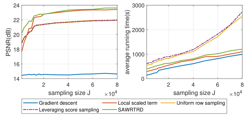
Figure 1: Average PSNR and running times versus sampling parameter $J$ using different strategies.

Both the decomposition and completion performance are evaluated using the Peak Signal-to-Noise Ratio (PSNR) between the original data and the recovered data. For each experiment, the PSNR value is averaged over 20 Monte Carlo runs with different noise realizations and missing locations. For the kernel width $\sigma$ in the proposed methods, we apply the adaptive kernel width selection strategy described in He et al. [2019]. The maximum number of iterations for all algorithms is set to $30$. The error tolerance $\epsilon$ of all algorithms is set to $10^{-3}$. All other parameters of the algorithms that we compare to are set to achieve their best performance in our experiments. All experiments were performed using MATLAB R2021a on a desktop PC with a 2.5-GHz processor and 32GB of RAM.

6.1 Ablation experiments

In this part, we carry out ablation experiments to verify the feasibility and advantage of the proposed strategies and also analyze the performance under different sampling sizes. The experiment is carried out using a color video ‘flamingo’ with resolution $1920\times 1080$ chosen from DAVIS 2016 dataset. The first $50$ frames are selected, so the video data can be represented as a $4$-dimensional tensor with size $1920\times 1080\times 3\times 50$. The data values are rescaled to $[0,1]$, and $30\%$ of the pixels are randomly and uniformly selected as the observed pixels. Then salt and pepper noise is added to the observed entries with probability $0.2$.

To demonstrate the advantage of the proposed methods, we develop four additional algorithms using different strategies. The first algorithm, referred to as ‘gradient descent’, uses the traditional gradient $d_{\mathcal{I}}(\mathbf{Z}_{k(2)})$ in (15) instead of $h_{\mathcal{I}}(\mathbf{Z}_{k(2)})$ in (16). The second algorithm, termed ‘local scaled term’, applies the local scaled term $\mathbf{G}_{\mathcal{Z}_{\mathcal{I}}^{\neq k}}$ from sampled core tensors $\{(\mathcal{Z}_{k})_{\mathcal{I}_{k}}\}_{k=1}^{N}$ to (16) instead of the global scaled term $\mathbf{G}_{\mathcal{Z}}^{\neq k}$. For the third algorithm, termed ‘uniform row sampling’, $\mathbf{Z}_{\mathcal{I}[2]}^{\neq k}$ is obtained using uniform row sampling [Malik and Becker, 2021] instead of RStS. In the fourth algorithm, referred to as ‘leverage score sampling’, the leverage score row sampling used in TRALS-S is directly applied. It should also be noticed that SAWRTRD without using FMGC is not included in the comparison, as it will be out of memory. Fig. 1 depicts the average PSNR and running times for five algorithms under different sampling sizes. The TR rank for all methods is set to [80, 80, 3, 20]. As can be seen, the values of PSNR for all algorithms are relatively stable for sample parameter $J\geq 4\times 10^{4}$. Also, the proposed RStS sampling strategy yields higher PSNR than the row sampling methods as well as lower computational cost. Further, the global scaled term outperforms the local scaled term, especially for small sampling size.

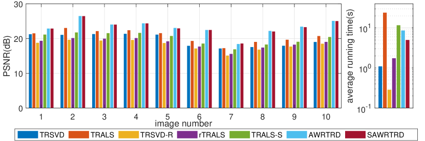
Figure 2: PSNR (left) for each image using different TR decomposition algorithms. Right: Average running time (right) of each algorithm on 10 images.

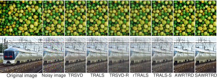
Figure 3: Recovered (cropped) images by different TR decomposition algorithms. Top: Image 2. Bottom: Image 7.

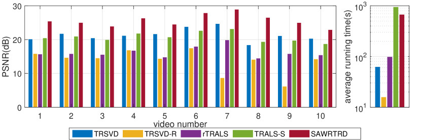
Figure 4: PSNR (left) for each video using different TR decomposition algorithms. Right: Average running time (right) of each algorithm on 10 videos.

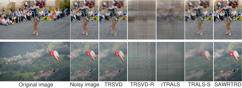
Figure 5: Recovered $10^{th}$ (cropped) frames by different TR decomposition algorithms. Top: Video 2. Bottom: Video 7.

6.2 High-resolution image/video TR decomposition with noise

In this part, we investigate the performance of TR decomposition in the presence of outliers. We first compare the decomposition performance on color image data. Specifically, 10 images are randomly selected from the DIV2K dataset [Agustsson and Timofte, 2017]. Two representative images are shown in Fig. 3. The height and width of the images are about $1350$ pixels and $2000$, respectively.

The values of the image data are rescaled to $[0,1]$, then two types of noise are added to the 10 images. Specifically, for the first 5 images, the noise is generated from a two-component Gaussian mixture model (GMM) with probability density function (PDF) $0.8N(0,10^{-3})+0.2N(0,0.5)$, where the latter term denotes the occurrence of outliers. For the last 5 images, $20\%$ of the pixels are perturbed with salt and pepper noise. The sampling parameter $J$ for SAWRTRD is set to $3\times 10^{4}$. The TR rank is set to $[20,20,3]$. For TRALS-S, the number of sampling rows for each mode is set to the same as SAWRTRD. The PSNR and average running time for different TR decomposition algorithms are shown in Fig. 2. As shown, the PSNR values of AWRTRD and SAWRTRD are always higher than the other algorithms. An example of the recovered images from the obtained core tensors is shown in Fig. 3. As shown, the images recovered by AWRTRD and SAWRTRD are visually better than the other algorithms.

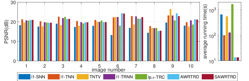
Figure 6: PSNR (left) for each image using different robust tensor completion algorithms. Right: Average running time (right) of each algorithm on 10 images.

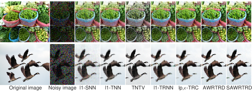
Figure 7: Recovered (cropped) images by different tensor completion algorithms. Top: Image 2. Bottom: Image 9.

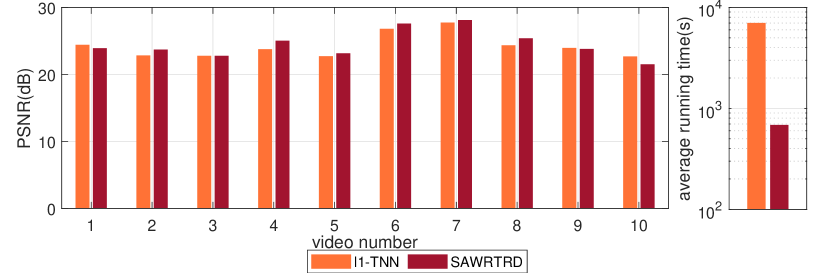
Figure 8: PSNR (left) for each video using different robust tensor completion algorithms. Right: Average running time (right) of each algorithm on 10 videos.

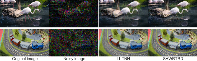
Figure 9: Recovered $10^{th}$ (cropped) frames by different tensor completion algorithms. Top: Video 5. Bottom: Video 10.

Then, we compare the decomposition performance of the proposed methods on video data. 10 videos with resolution $1920\times 1080$ are randomly chosen from the DAVIS 2016 dataset and the first $50$ frames are selected to form the tensor data. Representative frames from two videos are shown in Fig. 5. The values of the video data are rescaled to $[0,1]$, and the noises are added with distribution the same as in the previous experiment. Fig. 4 shows the PSNR and average running times using different robust tensor completion algorithms. Note that TRALS and AWRTRD are out of memory in the experiment, such that their results are not shown. As can be seen, the proposed SAWRTRD achieves significantly higher PSNR than other algorithms for all videos. Further, Fig. 5 illustrates the $10^{th}$ recovered frame of two videos. It can be seen that TRSVD-R and rTRALS fail to recover the frames, and the frames recovered by SAWRTRD have the clearest textures.

6.3 Image/video completion with noise

In this part, we compare the tensor completion performance of different robust tensor completion algorithms. Similar to the previous experiment, we randomly select 10 color images from DIV2K dataset, and 10 videos with the first $50$ frames from DAVIS 2016 dataset. The noises are added with distributions that are the same as in the previous experiment. Further, for each image and video, $30\%$ of the pixels are randomly and uniformly selected as the observed pixels. The sample parameter $J$ and the TR rank are set to $3\times 10^{4}$ and [80, 80, 3, 20], respectively. Fig.6 and Fig.8 report the PSNR and running times using different algorithms on images and videos, respectively. We should remark that only SAWRTRD and $\ell_{1}$-TNN can handle the video completion task while other algorithms run out of memory. As can be seen, in image completion, the proposed method can achieve comparable robust completion performance to other algorithms with significantly lower computational costs. For video completion, the performance of SAWRTRD and $\ell_{1}$-TNN are comparable, while the time cost of SAWRTRD is significantly smaller than $\ell_{1}$-TNN. Examples of the completed images and video frames are also given in Fig. 7 and Fig.9, respectively. Finally, we should remark that, unlike other robust tensor completion methods, our algorithm can also get compact TR representations of the images and videos.

7 Conclusion

We proposed a scalable and robust approach to TR decomposition. By introducing correntropy as the error measure, the proposed method can alleviate the impact of large outliers. Then, a simple auto-weighted robust TR decomposition algorithm was developed by leveraging an HQ technique and a scaled steepest descent method. We developed two strategies, FGMC and RStS, that exploit the special structure of the TR model to scale AWRTRD to large data. FGMC reduces the complexity of the underlying Gram matrix computation from exponential to linear, while RStS further reduces complexity by enabling the update of core tenors using a small sketch of the data. Experimental results demonstrate the superior performance of the proposed approach compared with existing TR decomposition and robust tensor completion methods.

References

- Agustsson and Timofte [2017] Eirikur Agustsson and Radu Timofte. Ntire 2017 challenge on single image super-resolution: Dataset and study. In The IEEE Conference on Computer Vision and Pattern Recognition (CVPR) Workshops, July 2017.
- Ahmadi-Asl et al. [2020] Salman Ahmadi-Asl, Andrzej Cichocki, Anh Huy Phan, Maame G Asante-Mensah, Mirfarid Musavian Ghazani, Toshihisa Tanaka, and Ivan Oseledets. Randomized algorithms for fast computation of low rank tensor ring model. Machine Learning: Science and Technology, 2(1):011001, 2020.
- Carroll and Chang [1970] J Douglas Carroll and Jih-Jie Chang. Analysis of individual differences in multidimensional scaling via an N-way generalization of “Eckart-Young” decomposition. Psychometrika, 35(3):283–319, 1970.
- Chen et al. [2013] Yi-Lei Chen, Chiou-Ting Hsu, and Hong-Yuan Mark Liao. Simultaneous tensor decomposition and completion using factor priors. IEEE Transactions on Pattern Analysis and Machine Intelligence, 36(3):577–591, 2013.
- Goldfarb and Qin [2014] Donald Goldfarb and Zhiwei Qin. Robust low-rank tensor recovery: Models and algorithms. SIAM Journal on Matrix Analysis and Applications, 35(1):225–253, 2014.
- Gu et al. [2014] Quanquan Gu, Huan Gui, and Jiawei Han. Robust tensor decomposition with gross corruption. Advances in Neural Information Processing Systems, 27, 2014.
- He et al. [2011] Ran He, Bao-Gang Hu, Wei-Shi Zheng, and Xiang-Wei Kong. Robust principal component analysis based on maximum correntropy criterion. IEEE Transactions on Image Processing, 20(6):1485–1494, 2011.
- He et al. [2014] Ran He, Baogang Hu, Xiaotong Yuan, Liang Wang, et al. Robust recognition via information theoretic learning. SpringerBriefs in Computer Science. Springer Cham, 2014.
- He et al. [2019] Yicong He, Fei Wang, Yingsong Li, Jing Qin, and Badong Chen. Robust matrix completion via maximum correntropy criterion and half-quadratic optimization. IEEE Transactions on Signal Processing, 68:181–195, 2019.
- Huang et al. [2020] Huyan Huang, Yipeng Liu, Zhen Long, and Ce Zhu. Robust low-rank tensor ring completion. IEEE Transactions on Computational Imaging, 6:1117–1126, 2020.
- Jiang and Ng [2019] Qiang Jiang and Michael Ng. Robust low-tubal-rank tensor completion via convex optimization. In IJCAI, pages 2649–2655, 2019.
- Kolda and Bader [2009] Tamara G Kolda and Brett W Bader. Tensor decompositions and applications. SIAM review, 51(3):455–500, 2009.
- Koren et al. [2009] Yehuda Koren, Robert Bell, and Chris Volinsky. Matrix factorization techniques for recommender systems. Computer, 42(8):30–37, 2009.
- Li et al. [2017] Ping Li, Jiashi Feng, Xiaojie Jin, Luming Zhang, Xianghua Xu, and Shuicheng Yan. Online robust low-rank tensor learning. In Proceedings of the 26th International Joint Conference on Artificial Intelligence, pages 2180–2186, 2017.
- Li and So [2021] Xiao Peng Li and Hing Cheung So. Robust low-rank tensor completion based on tensor ring rank via -norm. IEEE Transactions on Signal Processing, 69:3685–3698, 2021.
- Liu et al. [2007] Weifeng Liu, Puskal P Pokharel, and José C Príncipe. Correntropy: Properties and applications in non-Gaussian signal processing. IEEE Transactions on Signal Processing, 55(11):5286–5298, 2007.
- Malik and Becker [2021] Osman Asif Malik and Stephen Becker. A sampling-based method for tensor ring decomposition. In International Conference on Machine Learning, pages 7400–7411. PMLR, 2021.
- Nikolova and Ng [2005] Mila Nikolova and Michael K Ng. Analysis of half-quadratic minimization methods for signal and image recovery. SIAM Journal on Scientific computing, 27(3):937–966, 2005.
- Oseledets [2011] Ivan V Oseledets. Tensor-train decomposition. SIAM Journal on Scientific Computing, 33(5):2295–2317, 2011.
- Qiu et al. [2021] Duo Qiu, Minru Bai, Michael K Ng, and Xiongjun Zhang. Robust low-rank tensor completion via transformed tensor nuclear norm with total variation regularization. Neurocomputing, 435:197–215, 2021.
- Sidiropoulos et al. [2017] Nicholas D Sidiropoulos, Lieven De Lathauwer, Xiao Fu, Kejun Huang, Evangelos E Papalexakis, and Christos Faloutsos. Tensor decomposition for signal processing and machine learning. IEEE Transactions on Signal Processing, 65(13):3551–3582, 2017.
- Tanner and Wei [2016] Jared Tanner and Ke Wei. Low rank matrix completion by alternating steepest descent methods. Applied and Computational Harmonic Analysis, 40(2):417–429, 2016.
- Tucker [1966] Ledyard R Tucker. Some mathematical notes on three-mode factor analysis. Psychometrika, 31(3):279–311, 1966.
- Vervliet and De Lathauwer [2015] Nico Vervliet and Lieven De Lathauwer. A randomized block sampling approach to canonical polyadic decomposition of large-scale tensors. IEEE Journal of Selected Topics in Signal Processing, 10(2):284–295, 2015.
- Wang et al. [2020] Andong Wang, Zhong Jin, and Guoqing Tang. Robust tensor decomposition via t-svd: Near-optimal statistical guarantee and scalable algorithms. Signal Processing, 167:107319, 2020.
- Wang et al. [2017] Wenqi Wang, Vaneet Aggarwal, and Shuchin Aeron. Efficient low rank tensor ring completion. In Proceedings of the IEEE International Conference on Computer Vision, pages 5697–5705, 2017.
- Wang et al. [2016] Yulong Wang, Yuan Yan Tang, and Luoqing Li. Correntropy matching pursuit with application to robust digit and face recognition. IEEE transactions on cybernetics, 47(6):1354–1366, 2016.
- Yamaguchi and Hayashi [2017] Yuto Yamaguchi and Kohei Hayashi. Tensor decomposition with missing indices. In International Joint Conferences on Artificial Intelligence (IJCAI), volume 17, pages 3217–3223, 2017.
- Yang et al. [2015] Yuning Yang, Yunlong Feng, and Johan AK Suykens. Robust low-rank tensor recovery with regularized redescending M-estimator. IEEE Transactions on Neural Networks and Learning Systems, 27(9):1933–1946, 2015.
- Yu et al. [2019] Jinshi Yu, Chao Li, Qibin Zhao, and Guoxu Zhao. Tensor-ring nuclear norm minimization and application for visual: Data completion. In ICASSP 2019-2019 IEEE International Conference on Acoustics, Speech and Signal Processing (ICASSP), pages 3142–3146. IEEE, 2019.
- Yu et al. [2020] Jinshi Yu, Guoxu Zhou, Chao Li, Qibin Zhao, and Shengli Xie. Low tensor-ring rank completion by parallel matrix factorization. IEEE transactions on neural networks and learning systems, 32(7):3020–3033, 2020.
- Yuan et al. [2019] Longhao Yuan, Chao Li, Jianting Cao, and Qibin Zhao. Randomized tensor ring decomposition and its application to large-scale data reconstruction. In International Conference on Acoustics, Speech and Signal Processing (ICASSP), pages 2127–2131. IEEE, 2019.
- Zhao et al. [2016] Qibin Zhao, Guoxu Zhou, Shengli Xie, Liqing Zhang, and Andrzej Cichocki. Tensor ring decomposition. arXiv preprint arXiv:1606.05535, 2016.