Homogeneous Control Systems on Cones and Nonovershooting Finite-time Stabilizers

Abstract

A nonovershooting finite-time control design for linear multi-input system is proposed by upgrading a linear (asymptotic) nonovershooting stabilizer to a homogeneous one. Robustness of the safety and stability properties is analyzed using the concept of Input-to-State Stability (ISS) on invariant sets and Input-to-State Safety (ISSf). Theoretical results are illustrated on numerical examples.

1 Introduction

A tracking problem under certain state/output constrains can be solved using the so-called nonovershooting control [27] which, cast in the framework of control barrier functions [51], [3], [23], can be also employed for a ”safety filter” design, to override a potentially unsafe nominal controller [1, 39]. Linear and nonlinear nonovershooting controllers have been designed for both linear [35], [14], [12] and nonlinear systems [27], [28], [18]. The safety filter synthesis based on control barrier functions (CBF) has been extensively used in control applications such as automotive systems [2], [41] and multi-agent robotics [49], [45]. The barrier functions characterize positively invariant sets of safe control systems.

The positive invariance of closed sets for systems having unique solutions was first characterized in [31]. Control systems design (analysis) on invariant sets usually deals with compacts including a set-point (stable equilibrium) in its interior (as, for example, in [8]). The ellipsoidal and polyhedral invariant sets are the most popular in this context [9], [40]. For a nonovershooting stabilizer design, the desired set-point belongs to the boundary of the safe set. For linear systems, the corresponding invariant sets are linear positive cones and the nonovershooting property can be established by means of a transformation of the original system to a positive linear system [15], [13], [42] as, for example, in [39]. A nonlinear nonovershooting stabilizer design may be required even for linear control plant if, for example, some time constraints have to be fulfilled. Usually, the corresponding invariant set is not a linear cone and the related analysis is more complicated. This paper deals with a class of homogeneous systems, which admits a nonovershooting analysis similar to linear one.

Homogeneous system is a nonlinear system [53], [24], [43], [19], which, on the one hand, have many properties typical for linear systems such as equivalence of local and global results [7] or equivalence of asymptotic stability and Input-to-State Stability (ISS) with respect to homogeneously (resp., linearly) involved perturbations [44], [20]. On the other hand, they may demonstrate faster convergence [7], better robustness [4] and smaller overshoots [37, Chapter 1], [39]. A convergence rate of any stable homogeneous system is characterized by its homogeneity degree [32]. Homogeneity is a dilation symmetry widely studied in the group theory [17] and useful for control systems design [37]. Similarly to linear systems, invariant sets of homogeneous systems may be of a conic type (in a generalized sense). Therefore, analysis and design of nonovershooting homogeneous control systems should be developed on some homogeneous cones. This paper develops some tools for stability and robustness analysis of homogeneous systems on cones and provides a simple scheme of a nonovershooting finite-time stabilizer design for linear time-invariant multi-input plants.

The main contributions of the paper are as follows: the homogeneous Lyapunov function theorem [43] is refined for homogeneous systems on cones; the criterion of (robust) positive invariance [8], [5] is adapted to homogeneous cones; the homogeneous ISS theorem [44], [4] is extended to systems on cones; an algebraic condition of ISSf of homogeneous systems is obtained; an algorithm of non-overshooting finite-time stabilizer design is proposed for linear multi-input systems with linear conic constraints; ISS and ISSf of the obtained homogeneous non-overshooting control is proven. The paper is organized as follows. First, the problem statement and notions of interest are discussed. Next, some preliminaries about homogeneous systems are presented. After that, the issues of stability and robustness analysis of homogeneous systems on cones are studied and the nonovershooting homogeneous control is designed for linear plant. Finally, numerical examples and concluding remarks are given.

Notation. $\mathbb{R}$ is the field of reals, $\mathbb{R}_{+}=\{x\in\mathbb{R}:x\geq 0\}$ and $\mathbb{R}^{n}$ is the Euclidean space of column real vectors; $\|\cdot\|$ denotes a norm in $\mathbb{R}^{n}$ and $|\cdot|$ is the Euclidean norm in $\mathbb{R}^{n}$; we also use $\|\cdot\|_{\mathbb{R}^{k}}$ in order to highlight the dimension of the Euclidean space; $e_{i}=(0,\ldots,0,1,0,\ldots,0)^{\top}$ is the unit vector of the Euclidean basis in $\mathbb{R}^{n}$; $\partial\Omega$ denotes a boundary of $\Omega\subset\mathbb{R}^{n}$ and $\mathfrak{int}\,\Omega$ is the interior of $\Omega$; $C(\Omega,\mathbb{R}^{m})$ denotes a set of continuous mappings $\Omega\subset\mathbb{R}^{n}\mapsto\mathbb{R}^{m}$, where $\Omega$ is a connected set with non-empty interior; $C^{1}(\Omega,\mathbb{R}^{m})$ is a subset of mappings $C(\Omega,\mathbb{R}^{m})$, which are continuously differentiable on the interior of $\Omega$ such that all partial derivatives have a continuous prolongation to $\partial\Omega\cap\Omega$; we write shortly $C(\Omega)$ and $C^{1}(\Omega)$ if a context is clear or a dimension of the codomain is not important; $L^{\infty}(\mathbb{R},\mathbb{R}^{k})$ is a set of uniformly essentially bounded functions and $\|q\|_{L^{\infty}(t_{0},t_{1})}=\mathrm{ess}\sup_{t\in(t_{0},t_{1})}|q(t)|;$ $\mathcal{K}$ denotes the class of continuous strictly increasing functions $\sigma:[0,+\infty)\mapsto[0,+\infty)$ such that $\sigma(0)=0$; a function $\sigma\in\mathcal{K}$ is of the class $\mathcal{K}_{\infty}$ if $\sigma(s)\to+\infty$ as $s\to+\infty$; $\mathcal{KL}$ denotes the class of continuous functions $\beta:[0,+\infty)\times[0,+\infty)\mapsto[0,+\infty)$ such that $\beta(\cdot,t)$ is of class $\mathcal{K}$ for any $t\geq 0$ and the function $\beta(r,\cdot):[0,+\infty)\mapsto[0,+\infty]$ is decreasing such that $\beta(r,t)\to 0$ as $t\to+\infty$, for any $r\in[0,+\infty)$; for a symmetric matrix $P=P^{\top}\in\mathbb{R}^{n\times n}$, the order relation $P\succ 0$ (resp., $P\prec 0$) means that the matrix $P$ is positive (resp., negative) definite.

2 Problem Statement

Let us consider the system

(1) $$\dot{x}=f(x,q),\quad t>t_{0},\quad x(t_{0})=x_{0},$$

where $x(t)\in\mathbb{R}^{n}$ is the system state, $q\in L^{\infty}(\mathbb{R},\mathbb{R}^{k})$ is the exogenous input, and $f\in C(\mathbb{R}^{n}\times\mathbb{R}^{k},\mathbb{R}^{n})$. We consider the system (1) on a closed set

(2) $$\Omega=\{x\in\mathbb{R}^{n}\;:\;\phi_{i}(x)\geq 0,\;i=1,\ldots,p\},$$

with non-empty interior, where $\phi_{i}\in C(\mathbb{R}^{n},\mathbb{R})\cap C^{1}(\mathbb{R}^{n}\backslash\{\mathbf{0}\},\mathbb{R})$, $i=1,\ldots,p$, and study an asymptotic (or a finite-time) stability of the set

(3) $$\Omega_{0}=\{x\in\mathbb{R}^{n}:\phi_{i}(x)=0,\;i=1,2,\ldots,p\}$$

as well as Input-to-State Stability (ISS) of the system (1) on $\Omega$. In practice, the set $\Omega$ may define a safe set of the system (1). The functions $\phi_{i}$ are called the barrier functions in this case [3], [23]. For example, if the system (1) is globally asymptotically stable and the set $\Omega$ with $\phi_{1}(x)=x_{1},p=1$ is positively invariant for the system (1), then, obviously, all trajectories of the system initialized in $\Omega$ converge to $\Omega_{0}$ without overshoot in the first coordinate.

Below we assume that the set $\Omega$ has a topological characterization of a positive (in a generalized sense) cone. Recall that the (conventional) positive cone in a vector space is a set $\Xi$ such that $\lambda x\in\Xi$, $\forall\lambda>0$, $\forall x\in\Xi$. The positive cone $\Xi$ is linear if $x+y\in\Xi,\forall x,y\in\Xi$. Notice that the multiplication of a vector $x$ by a positive scalar $\lambda>0$ is the standard dilation in the vector space. The set $\Omega$ defines a standard positive cone in $\mathbb{R}^{n}$ if the functions $\phi_{i}$ are standard homogeneous $\phi_{i}(\lambda x)=\lambda^{\nu_{i}}\phi_{i}(x),\forall\lambda>0,\forall x\in\mathbb{R}^{n}$, where $\nu_{i}>0$ is the so-called homogeneity degree. To design a generalized positive cone in $\mathbb{R}^{n}$, a generalized dilation [53], [25], [43] can be utilized. Topological characterization of generalized dilations in Frechét and Euclidean spaces can be found in [22] and in [24], respectively. In this paper, we deal only with a cone $\Omega$ induced by means of the so-called linear dilation in $\mathbb{R}^{n}$ [36], [17]. The corresponding cone is usually nonlinear in $\mathbb{R}^{n}$, but it may become linear in a vector space homeomorphic to $\mathbb{R}^{n}$ (see Section 3). The system (1) is assumed to be generalized homogeneous (i.e., symmetric with respect to a generalized dilation) as well.

Definition 2.1.

The system (1) is said to be uniformly asymptotically stable on $\Omega$ if there exist $\beta_{i}\in\mathcal{KL}$ such that

(4) $$0\leq\phi_{i}(x(t))\leq\beta_{i}(|x_{0}|,t-t_{0}),\quad$$

for all $t\geq t_{0}$, $x_{0}\in\Omega$ and $i=1,\ldots,p$.

This definition introduces the asymptotic stability of the set $\Omega_{0}$ belonging to the boundary of the invariant set $\Omega$. Such a requirement is typical for the design of nonovershooting stabilizers and safety filters [27], [51], [1], [39]. Notice that if $\Omega$ is a homogeneous cone and the set $\Omega_{0}$ is bounded then $\Omega_{0}=\{\mathbf{0}\}$ (see Section 3 for more details). We study the robustness of the stability property of the system (1) on the cone $\Omega$ in the sense of the following definition inspired by [46], [29].

Definition 2.2.

The system (1) is said to be ISS on $\Omega$ if there exist $\beta_{i}\in\mathcal{KL}$ and $\gamma_{i}\in\mathcal{K}$ such that

(5) $$0\leq\phi_{i}(x(t))\leq\beta_{i}(|x_{0}|,t-t_{0})+\gamma_{i}(\|q\|_{L^{\infty}_{(t_{0},t)}}),\quad$$

for all $t\!\geq\!t_{0}$, $x_{0}\!\in\!\Omega$, $q\!\in\!L^{\infty}(\mathbb{R},\mathbb{R}^{k})$ and $i\!=\!1,\ldots,p$.

Our first aim is to obtain a characterization of ISS on $\Omega$ for a class of (generalized) homogeneous systems. The condition (5) looks similar to input-to-output stability (IOS) (see, e.g., [48]). In the general case, IOS is neither necessary nor sufficient for ISS on $\Omega$. However, the ISS on $\Omega$ may be equivalent to the regional ISS [29] provided that $\Omega$ is a compact and $x\to\mathbf{0}\Leftrightarrow\phi_{i}(x)\to\mathbf{0},\forall i=1,\ldots,p$. The left inequality in (5) simply means the set $\Omega$ is positively invariant for the system (1) independently of $q\in L^{\infty}$. This condition may be very restrictive in many practical cases. The concept of the Input-to-State Safety [26] relaxes the invariance of $\Omega$ as follows.

Definition 2.3.

The system (1) is said to be Input-to-State Safe (ISSf) on $\Omega$ if there exist $\gamma_{i}\in\mathcal{K}$ such that

(6) $$-\gamma_{i}\left(\|q\|_{L^{\infty}_{(t_{0},t)}}\right)\leq\phi_{i}(x(t))$$

for all $t\!\geq\!t_{0}$, $x_{0}\!\in\!\Omega$, $q\!\in\!L^{\infty}(\mathbb{R},\mathbb{R}^{k})$ and $i\!=\!1,\ldots,p$.

The inequality (6) simply means that the overshoot of the perturbed system must depend continuously on the magnitude of the perturbation. For robustness analysis of nonovershooting stabilizers, ISS on $\Omega$ and ISSf on $\Omega$ are merged as follows.

Definition 2.4.

The system (1) is said to be Input-to-State Safe and Stable (ISSfS) on $\Omega$ if there exist $\beta_{i}\in\mathcal{KL}$ and $\gamma_{i}\in\mathcal{K}$ such that

(7) $$-\gamma_{i}(\|q\|_{L^{\infty}_{(t_{0},t)}})\leq\phi_{i}(x(t))\leq\beta_{i}(|x_{0}|,t-t_{0})+\gamma_{i}(\|q\|_{L^{\infty}_{(t_{0},t)}}),\quad$$

for all $t\!\geq\!t_{0}$, $x_{0}\!\in\!\Omega$, $q\!\in\!L^{\infty}(\mathbb{R},\mathbb{R}^{k})$ and $i\!=\!1,\ldots,p$.

Our second aim is to characterize the robustness of both safety and stability properties of the system (1) on the cone $\Omega$ in the sense of the latter definition.

The final goal of the paper is to design a nonovershooting finite-time stabilizer for a nonlinear generalized homogeneous system using its unperturbed linear model,

$$\dot{x}=f(x,\mathbf{0})=Ax+Bu(x),$$

where $x$ is as before, $A\in\mathbb{R}^{n\times n}$, $B\in\mathbb{R}^{n\times m}$ and $u:\mathbb{R}^{n}\mapsto\mathbb{R}^{m}$ is a nonovershooting finite-time stabilizer to be designed for a certain class of generalized homogeneous cones $\Omega$ defined below. The robustness (with respect to additive perturbations and measurement noises) of stability and safety properties of the closed-loop system is going to be studied in the sense of the above definitions.

3 Generalized Homogeneity in $\mathbb{R}^{n}$

3.1 Linear dilations

Let us recall that a family of operators $\mathbf{d}(s):\mathbb{R}^{n}\mapsto\mathbb{R}^{n}$ with $s\in\mathbb{R}$ is a group if $\mathbf{d}(0)x\!=\!x$, $\mathbf{d}(s)\!\circ\!\mathbf{d}(t)x\!=\!\mathbf{d}(s\!+\!t)x$, $\forall x\!\in\!\mathbb{R}^{n},\forall s,t\!\in\!\mathbb{R}$. A group $\mathbf{d}$ is a) continuous if the mapping $s\mapsto\mathbf{d}(s)x$ is continuous, $\forall x\!\in\!\mathbb{R}^{n}$; b) linear if $\mathbf{d}(s)$ is a linear mapping (i.e., $\mathbf{d}(s)\in\mathbb{R}^{n\times n}$), $\forall s\in\mathbb{R}$; c) a dilation in $\mathbb{R}^{n}$ if $\liminf\limits_{s\to+\infty}\|\mathbf{d}(s)x\|=+\infty$ and $\limsup\limits_{s\to-\infty}\|\mathbf{d}(s)x\|=0$, $\forall x\neq\mathbf{0}$. Any linear continuous group in $\mathbb{R}^{n}$ admits the representation [34]

(8) $$\mathbf{d}(s)=e^{sG_{\mathbf{d}}}=\sum_{j=1}^{\infty}\tfrac{s^{j}G_{\mathbf{d}}^{j}}{j!},\quad s\in\mathbb{R},$$

where $G_{\mathbf{d}}\in\mathbb{R}^{n\times n}$ is a generator of $\mathbf{d}$. A continuous linear group (8) is a dilation in $\mathbb{R}^{n}$ if and only if $G_{\mathbf{d}}$ is an anti-Hurwitz matrix [36]. In this paper we deal only with continuous linear dilations. A dilation $\mathbf{d}$ in $\mathbb{R}^{n}$ is a) monotone if the function $s\mapsto\|\mathbf{d}(s)x\|$ is strictly increasing, $\forall x\neq\mathbf{0}$; b) strictly monotone if $\exists\beta\!>\!0$ such that $\|\mathbf{d}(s)x\|\!\leq\!e^{\beta s}\|x\|$, $\forall s\!\leq\!0$, $\forall x\in\mathbb{R}^{n}$. The following result is the straightforward consequence of the existence of the quadratic Lyapunov function for asymptotically stable LTI systems.

Corollary 3.1.

A linear continuous dilation in $\mathbb{R}^{n}$ is strictly monotone with respect to the weighted Euclidean norm $\|x\|=\sqrt{x^{\top}Px},0\prec P\in\mathbb{R}^{n\times n}$ if and only if

(9) $$PG_{\mathbf{d}}+G_{\mathbf{d}}^{\top}P\succ 0,\quad P\succ 0.$$

Any dilation in $\mathbb{R}^{n}$ defines an alternative topology (balls, spheres, cones, etc) in $\mathbb{R}^{n}$. Below we study the systems on generalized homogeneous cones.

Definition 3.2.

Let $\mathbf{d}$ be a dilation in $\mathbb{R}^{n}$. A nonempty set $\mathcal{D}\subset\mathbb{R}^{n}$ is said to be $\mathbf{d}$-homogeneous cone if $\mathbf{d}(s)\mathcal{D}\subset\mathcal{D}$ for all $s\in\mathbb{R}$.

A standard homogeneous cone (i.e., $\mathbf{d}_{1}(s)=e^{s}I_{n}$) and the generalized homogeneous cone are illustrated on Fig. 1.

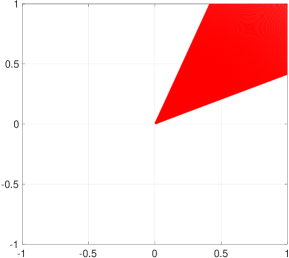
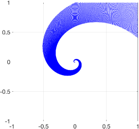
Figure 1: Standard and generalized homogeneous cones

Notice that if $\mathcal{D}\subset\mathbb{R}^{n}$ is a non-empty closed $\mathbf{d}$-homogeneous cone then $\mathbf{0}\in\mathcal{D}$. Indeed, if $x\in\mathcal{D},x\neq\mathbf{0}$ then $\mathbf{d}(s)x\in\mathcal{D},\forall s\in\mathbb{R}$ and $\mathbf{d}(s)x\to\mathbf{0}$ as $s\to-\infty$. Since $\mathcal{D}$ is closed then the limit point $\mathbf{0}$ belongs to $\mathcal{D}$. Below we deal only with a linear continuous dilation $\mathbf{d}$ in $\mathbb{R}^{n}$.

3.2 Canonical homogeneous norm

Any linear continuous and monotone dilation in a normed vector space introduces also an alternative norm topology defined by the so-called canonical homogeneous norm [36].

Definition 3.3 (Canonical homogeneous norm).

Let a linear dilation $\mathbf{d}$ in $\mathbb{R}^{n}$ be continuous and monotone with respect to a norm $\|\cdot\|$. A function $\|\cdot\|_{\mathbf{d}}:\mathbb{R}^{n}\mapsto[0,+\infty)$ defined as follows: $\|\mathbf{0}\|_{\mathbf{d}}=0$ and

(10) $$\|x\|_{\mathbf{d}}=e^{s_{x}},\;\text{where}\;s_{x}\in\mathbb{R}:\|\mathbf{d}(-s_{x})x\|=1,\quad x\neq\mathbf{0}\vspace{-1mm}$$

is said to be a canonical $\mathbf{d}$-homogeneous norm in $\mathbb{R}^{n}$

For standard dilation $\mathbf{d}_{1}(s)=e^{s}I_{n}$ we, obviously, have $\|x\|_{\mathbf{d}_{1}}=\|x\|$. In other cases, $\|x\|_{\mathbf{d}}$ with $x\neq\mathbf{0}$ is implicitly defined by a nonlinear algebraic equation, which always have a unique solution due to monotonicity of the dilation. In some particular cases [39], this implicit equation has explicit solution even for non-standard dilations.

Lemma 3.4.

[36] If a linear continuous dilation $\mathbf{d}$ in $\mathbb{R}^{n}$ is monotone with respect to a norm $\|\cdot\|$ then

• $\|\cdot\|_{\mathbf{d}}:\mathbb{R}^{n}\mapsto\mathbb{R}_{+}$ is single-valued and continuous on $\mathbb{R}^{n}$;

• there exist $\sigma_{1},\sigma_{2}\in\mathcal{K}_{\infty}$ such that

  (11) $$\sigma_{1}(\|x\|_{\mathbf{d}})\leq\|x\|\leq\sigma_{2}(\|x\|_{\mathbf{d}}),\quad\quad\forall x\in\mathbb{R}^{n};$$

• $\|\cdot\|$ is locally Lipschitz continuous on $\mathbb{R}^{n}\backslash\{\mathbf{0}\}$ provided that the linear dilation $\mathbf{d}$ is strictly monotone ;

• $\|\cdot\|_{\mathbf{d}}$ is continuously differentiable on $\mathbb{R}^{n}\backslash\{\mathbf{0}\}$ provided that $\|\cdot\|$ is continuously differentiable on $\mathbb{R}^{n}\backslash\{\mathbf{0}\}$ and $\mathbf{d}$ is strictly monotone.

For the $\mathbf{d}$-homogeneous norm $\|x\|_{\mathbf{d}}$ induced by the weighted Euclidean norm $\|x\|=\sqrt{x^{\top}Px}$ we have [36]

(12) $$\tfrac{\partial\|x\|_{\mathbf{d}}}{\partial x}=\|x\|_{\mathbf{d}}\tfrac{x^{\top}\mathbf{d}^{\top}(-\ln\|x\|_{\mathbf{d}})P\mathbf{d}(-\ln\|x\|_{\mathbf{d}})}{x^{\top}\mathbf{d}^{\top}(-\ln\|x\|_{\mathbf{d}})PG_{\mathbf{d}}\mathbf{d}(-\ln\|x\|_{\mathbf{d}})x}.$$

If $\mathbf{d}$ is a linear continuous strictly monotone dilation then the mapping $\Psi:\mathbb{R}^{n}\mapsto\mathbb{R}^{n}$,

(13) $$\Psi(x)=\|x\|_{\mathbf{d}}\mathbf{d}(-\ln\|x\|_{\mathbf{d}})x,\quad x\in\mathbb{R}^{n}\backslash\{\mathbf{0}\}$$

is a homeomorphism in $\mathbb{R}^{n}$, its inverse is given by $\Psi^{-1}(z)=\|z\|^{-1}\mathbf{d}(\ln\|z\|)z,\quad z\in\mathbb{R}^{n}\backslash\{\mathbf{0}\}$, with the prolongation $\Psi(\mathbf{0})=\Psi^{-1}(\mathbf{0})=\mathbf{0}$ by continuity. If $\|\cdot\|$ is differentiable on $\mathbb{R}^{n}\backslash\{\mathbf{0}\}$ then $\Psi$ is diffeomorphism on $\mathbb{R}^{n}\backslash\{\mathbf{0}\}$.

Theorem 3.5.

[37] Let a linear continuous dilation $\mathbf{d}$ in $\mathbb{R}^{n}$ be monotone with respect to a norm $\|\cdot\|$. Let an addition operation $\tilde{+}:\mathbb{R}^{n}\times\mathbb{R}^{n}\mapsto\mathbb{R}^{n}$ and a multiplication by a scalar $\tilde{\cdot}:\mathbb{R}\times\mathbb{R}^{n}\mapsto\mathbb{R}^{n}$ be defined as follows

• $x\tilde{+}y:=\Psi^{-1}(\Psi(x)+\Psi(y))$, where $x,y\in\mathbb{R}^{n}$,

• $\lambda\tilde{\cdot}x:=\mathrm{sign}(\lambda)\mathbf{d}(\ln|\lambda|)x$, where $\lambda\in\mathbb{R}$, $x\in\mathbb{R}^{n}$,

where $\Psi:\mathbb{R}^{n}\mapsto\mathbb{R}^{n}$ is given by (13). Then the set $\mathbb{R}^{n}$ together with the operations $\tilde{+}$ and $\tilde{\cdot}$ is a linear vector space $\mathbb{R}^{n}_{\mathbf{d}}$ with the norm $\|\cdot\|_{\mathbf{d}}$.

The latter theorem justifies the name norm for $\|\cdot\|_{\mathbf{d}}$. Notice that $\mathbf{d}$-homogeneous cones are usually nonlinear in $\mathbb{R}^{n}$ (see Fig. 1), but they may be linear in $\mathbb{R}^{n}_{\mathbf{d}}$.

Corollary 3.6.

For any $h_{i}\in\mathbb{R}^{n},i=1,\ldots,p$ the set

(14) $$\Omega_{\rm lin}=\{x\in\mathbb{R}^{n}:h_{i}^{\top}{\Psi(x)}\geq 0,i=1,\ldots,p\}$$

is a linear positive cone in the space $\mathbb{R}^{n}_{\mathbf{d}}$.

Proof 3.7.

Indeed, since for $x,y\in\Omega_{\rm lin}$ we have $h_{i}^{\top}\Psi(x)\geq 0$, $h_{i}^{\top}\Psi(y)\geq 0$ for all $i=1,\ldots,p$ then using $x\tilde{+}y=\Psi^{-1}(\Psi(x)+\Psi(y))$ we derive $h_{i}^{\top}\Psi(x\tilde{+}y)=h_{i}^{\top}\Psi(x)+h_{i}^{\top}\Psi(y)\geq 0\quad\Rightarrow\quad x\tilde{+}y\in\Omega_{\rm lin}.$

3.3 Homogeneous functions and vector fields

Below we study systems that are symmetric on homogeneous cones with respect to a linear dilation $\mathbf{d}$. The dilation symmetry introduced by the following definition is known as a generalized homogeneity [53], [24], [43], [7], [37].

Definition 3.8.

[24] A function $h:\mathbb{R}^{n}\mapsto\mathbb{R}$ is $\mathbf{d}$-homogeneous of degree $\nu\!\in\!\mathbb{R}$ if

$$h(\mathbf{d}(s)x)=e^{\nu s}h(x),\quad\forall x\in\mathbb{R}^{n},\quad\forall s\in\mathbb{R}.$$

Notice that $h(x)=\|x\|_{\mathbf{d}}^{\nu}h(\mathbf{d}(-\ln\|x\|_{\mathbf{d}})x),\forall x\neq\mathbf{0}$ for any $\mathbf{d}$-homogeneous function $h$ of degree $\nu$, where $\|\cdot\|_{\mathbf{d}}$ is a canonical homogeneous norm induced by a norm $\|\cdot\|$ in $\mathbb{R}^{n}$, so $\|\mathbf{d}(-\ln\|x\|_{\mathbf{d}})x\|=1,\forall x\neq\mathbf{0}$. The latter implies that if a $\mathbf{d}$-homogeneous function $h$ is continuous at zero then either $h\equiv{\rm const}$ or $h(\mathbf{0})=0$ and $\nu>0$. So, non-constant continuous $\mathbf{d}$-homogeneous functions $\phi_{i}$ may define a $\mathbf{d}$-homogeneous cone $\Omega$ given by (2) if and only if they have positive homogeneity degree.

Assumption 1.

Let $\phi_{i}\in C(\mathbb{R}^{n},\mathbb{R})\cap C^{1}(\mathbb{R}^{n}\backslash\{\mathbf{0}\})$ in (2) be $\mathbf{d}$-homogeneous of degree $\nu_{i}>0$, $i=1,2,\ldots,p$

The set $\Omega_{i}=\{x\in\mathbb{R}^{n}:\phi_{i}(x)\geq 0\}$ with $\phi_{i}$ satisfying this assumption is a $\mathbf{d}$-homogeneous cone with a smooth boundary everywhere except, probably, the origin. The set $\Omega=\bigcap\limits_{i=1}^{p}\Omega_{i}$ given by (2) is also a $\mathbf{d}$-homogeneous cone.

Assumption 2.

The set $\Omega_{0}$ given by (3) is bounded.

Since $\Omega_{0}$ is a $\mathbf{d}$-homogeneous cone, then the boundedness of $\Omega_{0}$ means that

(15) $$\Omega_{0}\!=\!\{\mathbf{0}\}.$$

Indeed, otherwise, the set $\Omega_{0}$ is unbounded since $\mathbf{d}(s)x\in\Omega_{0},\forall x\in\Omega_{0},\forall s\in\mathbb{R}$, but $\|\mathbf{d}(s)x\|\to+\infty$ as $s\to+\infty$ for any $x\neq\mathbf{0}$. Below we study the systems on $\mathbf{d}$-homogeneous cones $\Omega$ with both bounded and unbounded sets $\Omega_{0}$.

Definition 3.9.

[24] A vector field $f:\mathbb{R}^{n}\mapsto\mathbb{R}^{n}$ is $\mathbf{d}$-homogeneous of degree $\mu\in\mathbb{R}$ if

(16) $$g(\mathbf{d}(s)x)=e^{\mu s}\mathbf{d}(s)g(x),\quad\quad\forall s\in\mathbb{R},\quad\forall x\in\mathbb{R}^{n}.$$

Formally, to avoid a collision in Definitions 3.8 and 3.9 for $n=1$, a vector field $g$ should be defined as $g:\Xi\mapsto T\Xi$, where $T\Xi$ is the tangent space for $\Xi$. Since the tangent space of $\mathbb{R}^{n}$ is associated with $\mathbb{R}^{n}$, we simply write $g:\mathbb{R}^{n}\mapsto\mathbb{R}^{n}$.

The homogeneity of a mapping is inherited by other mathematical objects induced by this mapping. In particular, solutions of $\mathbf{d}$-homogeneous system

(17) $$\dot{x}=g(x),\quad t>0,\quad x(0)=x_{0}\in\mathbb{R}^{n}$$

are symmetric with respect to the dilation $\mathbf{d}$ in the following sense [53], [24], [7]

(18) $$x(t,\mathbf{d}(s)x_{0})=\mathbf{d}(s)x(e^{\mu s}t,x_{0}),$$

where $x(\cdot,z)$ denotes a solution of (17) with $x(0)=z\in\mathbb{R}^{n}$ and $\mu\in\mathbb{R}$ is the homogeneity degree of $g$. The mentioned symmetry of solutions implies many useful properties of homogeneous system such as equivalence of local and global results (e.g, about existence, uniqueness and stability solutions) or finite-time stability of any asymptotically stable $\mathbf{d}$-homogeneous system (17) with negative degree [7].

Corollary 3.10.

If $g\in C(\mathbb{R}^{n})$ is a $\mathbf{d}$-homogeneous vector field of degree $\mu\leq 0$ then the system (17) is forward complete.

Proof 3.11.

By Corollary 3.1, any linear continuous dilation is strictly monotone with respect to the weighted Euclidean norm $\|x\|=\sqrt{x^{\top}Px}$ with P satisfying (9). Let $\|\cdot\|_{\mathbf{d}}$ be the canonical homogeneous norm induced by $\|\cdot\|$. Then using (12) and $\mathbf{d}$-homogeneity of $g$ we derive

$$\tfrac{d}{dt}\|x\|_{\mathbf{d}}=\|x\|_{\mathbf{d}}\tfrac{x^{\top}\mathbf{d}^{\top}(-\ln\|x\|_{\mathbf{d}})P\mathbf{d}(-\ln\|x\|_{\mathbf{d}})\dot{x}}{x^{\top}\mathbf{d}^{\top}(-\ln\|x\|_{\mathbf{d}})PG_{\mathbf{d}}\mathbf{d}(-\ln\|x\|_{\mathbf{d}})x}=\|x\|^{1+\mu}_{\mathbf{d}}\tilde{g}(\mathbf{d}(-\ln\|x\|_{\mathbf{d}})x),$$

where $\tilde{g}(z)=\tfrac{z^{\top}Pg(z)}{z^{\top}PG_{\mathbf{d}}z}$, $z\in\mathbb{R}^{n}$. Taking into account $\|\mathbf{d}(-\ln\|x\|_{\mathbf{d}})x\|=1$ we conclude $\exists\gamma>0:\|\tilde{g}(\mathbf{d}(-\ln\|x\|_{\mathbf{d}})x)\|\leq\gamma=\sup_{\|z\|=1}\|\tilde{g}(z)\|<+\infty$ for all $x\neq\mathbf{0}$ and $\tfrac{d}{dt}\|x\|_{\mathbf{d}}\leq\gamma\|x\|^{1+\mu}_{\mathbf{d}},\quad\forall x\neq\mathbf{0}.$ For $\mu\leq 0$ the obtained differential inequality guarantees that the system (17) is forward complete.

The well-known Euler’s homogeneous function theorem proves that the derivative of any smooth standard homogeneous function $h(e^{s}x)=e^{\nu s}h(x)$ is homogeneous and $\frac{\partial h(x)}{\partial x}x=\nu f(x),\forall x\in\mathbb{R}^{n}$. An analog of the Euler’s theorem for $\mathbf{d}$-homogeneous vector fields is given below.

Theorem 3.12.

[37] If $h\!\in\!C^{1}(\mathbb{R}^{n}\backslash\{\mathbf{0}\},\mathbb{R})$ is $\mathbf{d}$-homogeneous function of degree $\nu\in\mathbb{R}$ then

(19) $$\tfrac{\partial h(x)}{\partial x}G_{\mathbf{d}}x=\nu h(x),\quad\forall x\neq\mathbf{0},$$

(20) $$\left.\tfrac{\partial h(z)}{\partial z}\right|_{z=\mathbf{d}(s)x}\mathbf{d}(s)=e^{\nu s}\tfrac{\partial h(x)}{\partial x},\quad\forall x\neq\mathbf{0},\quad\forall s\in\mathbb{R}.$$

If $g\in C^{1}(\mathbb{R}^{n}\backslash\{\mathbf{0}\},\mathbb{R}^{n})$ is a $\mathbf{d}$-homogeneous vector field of degree $\mu\in\mathbb{R}$ then

(21) $$\tfrac{\partial g(x)}{\partial x}G_{\mathbf{d}}x=(\mu I_{n}+G_{\mathbf{d}})g(x),\quad\forall x\neq\mathbf{0},$$

(22) $$\left.\tfrac{\partial g(z)}{\partial z}\right|_{z=\mathbf{d}(s)x}\mathbf{d}(s)=e^{\mu s}\mathbf{d}(s)\tfrac{\partial g(x)}{\partial x},\quad\forall x\neq\mathbf{0},\quad\forall s\in\mathbb{R}.$$

The perturbed homogeneous system (1) under consideration is characterized by the following assumption inspired by [44], [20], [4].

Assumption 3.

Let a linear continuous dilation $\mathbf{d}$ in $\mathbb{R}^{n}$ be monotone with respect to a norm $\|\cdot\|_{\mathbb{R}^{n}}$, and a linear continuous dilation $\tilde{\mathbf{d}}$ in $\mathbb{R}^{k}$ be monotone with respect to a norm $\|\cdot\|_{\mathbb{R}^{k}}$. Let the vector field $\hat{f}\in C(\mathbb{R}^{n+k})$ given by

$$\hat{f}(x,q)=\left(\begin{array}[]{c}f(x,q)\\ \mathbf{0}\end{array}\right),\quad x\in\mathbb{R}^{n},\quad q\in\mathbb{R}^{k},$$

be $\hat{\mathbf{d}}$-homogeneous of degree $\mu>-1$, where $\hat{\mathbf{d}}(s)=\left(\begin{smallmatrix}\mathbf{d}(s)&\mathbf{0}\\ \mathbf{0}&\tilde{\mathbf{d}}(s)\end{smallmatrix}\right),s\in\mathbb{R}.$

A certain dilation symmetry can be discovered for solutions of the perturbed homogeneous system as well (see, e.g., [38]).

Lemma 3.13.

Let $x_{q}(t,x_{0})$, $t\geq t_{0}$ denote a solution of the system (1). Let $x_{q_{s}}(t,\mathbf{d}(s)x_{0})$, $t\geq t_{0}$ denote a solution of the system (1) for $x_{0}\in\mathbb{R}^{n}$ replaced with $\mathbf{d}(s)x_{0}\in\mathbb{R}^{n},s\in\mathbb{R}$ and $q\in L^{\infty}(\mathbb{R},\mathbb{R}^{n})$ replaced with $q_{s}\in L^{\infty}(\mathbb{R},\mathbb{R}^{k})$ given by

(23) $$q_{s}(t)=\tilde{\mathbf{d}}(s)q(t_{0}+e^{\mu s}(t-t_{0})),\quad\forall t\in\mathbb{R}.$$

Then, under Assumption 3, the identity

(24) $$x_{q_{s}}(t,\mathbf{d}(s)x_{0})\!=\!\mathbf{d}(s)x_{q}(t_{0}+e^{\mu s}(t-t_{0}),x_{0}),\quad t\geq t_{0},$$

holds as long as solutions exist.

Proof 3.14.

Indeed, denoting $\tau=t_{0}+e^{\mu s}(t-t_{0})$ we obtain

$$\frac{d}{dt}\mathbf{d}(s)x_{q}(t_{0}+e^{\mu s}(t-t_{0}),x_{0})=e^{\mu s}\mathbf{d}(s)\frac{d}{d\tau}x_{q}(\tau,x_{0})=e^{\mu s}\mathbf{d}(s)f(x_{q}(\tau),q(\tau)).$$

Using the $\hat{\mathbf{d}}$-homogeneity of $\hat{f}$ we derive

$$\frac{d}{dt}\mathbf{d}(s)x_{q}(t_{0}+e^{\mu s}(t-t_{0}),x_{0})\!=\!f(\mathbf{d}(s)x_{q}(t_{0}+e^{\mu s}(t-t_{0}),x_{0}),\tilde{\mathbf{d}}(s)q(t_{0}+e^{\mu s}(t-t_{0})))$$

Since $\frac{d}{dt}x_{q_{s}}(t,\mathbf{d}(s)x_{0})=f(x_{q_{s}}(t,\mathbf{d}(s)x_{0}),q_{s}(t))$, then the identity (24) holds.

If solutions of the perturbed system (1) are not unique then the identity (24) is understood in the set-theoretic sense: the set of solutions is invariant up to certain scaling of initial condition, time and the perturbation function $q$.

4 Homogeneous Systems on Cones

4.1 Positively Invariant Homogeneous Cones

The criterion of the positive invariance of a closed set $\Omega\subset\mathbb{R}^{n}$ is well known in the literature (see, e.g., [31], [5], [8]): if the forward complete system (17) has a unique solution for any $x_{0}\in\Omega$ then the closed set $\Omega$ is positively invariant for the system (17) if and only if

(25) $$g(x)\in\mathcal{C}_{\Omega}(x),\quad\forall x\in\Omega,$$

where $\mathcal{C}_{\Omega}(x)\subset\mathbb{R}^{n}$ is the (Bouligand) tangent cone to $\Omega$ at $x\in\mathbb{R}^{n}$ defined as

(26) $$\mathcal{C}_{\Omega}(x)=\left\{z\in\mathbb{R}^{n}:\liminf_{h\to 0^{+}}\tfrac{\inf_{y\in\Omega}\|x+hz-y\|}{h}=0\right\}.$$

Obviously, $\mathcal{C}_{\Omega}(x)$ is a positive cone ($z\in\mathcal{C}_{\Omega}(x)\Rightarrow\lambda z\in\mathcal{C}_{\Omega}(x),\forall\lambda>0$). Notice that $\mathcal{C}_{\Omega}(x)=\{\emptyset\}$ for $x\notin\Omega$ and $\mathcal{C}_{\Omega}(x)=\mathbb{R}^{n}$ for $x\in\mathfrak{int}\,\Omega$, so the condition (25) can be relaxed to $x\in\partial\Omega$. The homogeneity of the set $\Omega$ implies the homogeneity of the tangent cone $\mathcal{C}_{\Omega}(x)$.

Lemma 4.1.

If $\Omega\subset\mathbb{R}^{n}$ is a closed $\mathbf{d}$-homogeneous cone then

(27) $$\mathcal{C}_{\Omega}(\mathbf{d}(s)x)=\mathbf{d}(s)\mathcal{C}_{\Omega}(x),\quad\forall x\in\Omega,\quad\forall s\in\mathbb{R}.$$

Proof 4.2.

On the one hand, we have

$$\mathcal{C}_{\Omega}(\mathbf{d}(s)x)=\left\{z\in\mathbb{R}^{n}:\liminf_{h\to 0^{+}}\tfrac{\inf_{y\in\Omega}\|\mathbf{d}(s)x+hz-y\|}{h}=0\right\}$$

$$=\left\{\mathbf{d}(s)\tilde{z}\in\mathbb{R}^{n}:\liminf_{h\to 0^{+}}\tfrac{\inf_{\mathbf{d}(s)\tilde{y}\in\Omega}\|\mathbf{d}(s)(x+h\tilde{z}-\tilde{y})\|}{h}=0\right\}$$

$$=\mathbf{d}(s)\left\{\tilde{z}\in\mathbb{R}^{n}:\liminf_{h\to 0^{+}}\tfrac{\inf_{\tilde{y}\in\Omega}\|\mathbf{d}(s)(x+h\tilde{z}-\tilde{y})\|}{h}=0\right\}$$

where the $\mathbf{d}$-homogeneity of $\Omega$ (i.e., $\mathbf{d}(s)\Omega\subset\Omega,\forall s\in\mathbb{R}$) is utilized on the last step. On the other hand, the set $\mathcal{C}_{\Omega}(x)$ is independent of the selection of a norm [31], [8]. Since $\mathbf{d}(s)$ is invertible then $\|\cdot\|_{*}=\|\mathbf{d}(s)\cdot\|$ is a norm in $\mathbb{R}^{n}$ and

$$\mathcal{C}_{\Omega}(x)=\left\{\tilde{z}\in\mathbb{R}^{n}:\liminf_{h\to 0^{+}}\tfrac{\inf_{\tilde{y}\in\Omega}\|\mathbf{d}(s)(x+h\tilde{z}-\tilde{y})\|}{h}=0\right\}.$$

The proof is complete.

In the view of the latter lemma, the positive invariance of a homogeneous cone for a homogeneous system can be analyzed considering the tangent cone and the vector field on the unit sphere.

Corollary 4.3.

Let a linear continuous dilation $\mathbf{d}$ be monotone with respect to a norm $\|\cdot\|$ in $\mathbb{R}^{n}$ and a vector field $g\in C(\mathbb{R}^{n})$ be $\mathbf{d}$-homogeneous of degree $\mu\in\mathbb{R}$ such that $g(\mathbf{0})=\mathbf{0}$, solutions of the system (17) are forward unique and complete on $\Omega$. A closed $\mathbf{d}$-homogeneous cone $\Omega$ is positively invariant for (17) if and only if

(28) $$g(x)\in\mathcal{C}_{\Omega}(x),\quad\forall x\in\partial\Omega\cap S,$$

where $S=\{x\in\mathbb{R}^{n}:\|x\|=1\}$ is the unit sphere.

Proof 4.4.

For any $x\neq\mathbf{0}$, due to $\mathbf{d}$-homogeneity of $g$ and $\mathcal{C}_{\Omega}$ (see Lemma 4.1), we have

$$g(x)=\|x\|^{-\mu}_{\mathbf{d}}\mathbf{d}(\ln\|x\|_{\mathbf{d}})g(\mathbf{d}(-\ln\|x\|_{\mathbf{d}})x)\text{ and }\mathcal{C}_{\Omega}(x)=\mathbf{d}(\ln\|x\|_{\mathbf{d}})\mathcal{C}_{\Omega}(\mathbf{d}(-\ln\|x\|_{\mathbf{d}})x).$$

Hence, the condition (28) implies $g(x)\in\mathcal{C}_{\Omega}(x),\quad\forall x\in\partial\Omega\backslash\{\mathbf{0}\},$ which is necessary and sufficient for the set $\Omega\backslash\{\mathbf{0}\}$ to be positively invariant (at least, as long as $x(t)\neq\mathbf{0}$). On the one hand, since the $\mathbf{d}$-homogeneous cone is closed then $\mathbf{0}\in\Omega$. On the other hand, since $g(\mathbf{0})=\mathbf{0}$ then, taking into account the forward uniqueness of the zero solution, we complete the proof.

The positive invariance of a “linear” $\mathbf{d}$-homogeneous cone $\Omega_{\rm lin}$ admits a more simple algebraic characterization.

Corollary 4.5.

Let, under conditions of Corollary 4.3, the norm in $\mathbb{R}^{n}$ be defined as $\|x\|=\sqrt{z^{\top}Pz}$ with $P\in\mathbb{R}^{n\times n}$ satisfying (9). The $\mathbf{d}$-homogeneous cone $\Omega=\Omega_{\rm lin}$ given by (14) is positively invariant for the system (17) if and only if

(29) $$h_{i}^{\top}g(z)\geq\tfrac{z^{\top}Pg(z)}{z^{\top}PG_{\mathbf{d}}z}h_{i}^{\top}G_{\mathbf{d}}z,\quad\forall z\in\Xi_{i},\quad\forall i=1,\ldots,p,$$

where $\Xi_{i}:=\{z\in\mathbb{R}^{n}:\|z\|=1,h_{i}^{\top}z=0,h^{\top}_{j}z\geq 0,\forall j\neq i\}$.

Proof 4.6.

In the new coordinates $z=\Psi(x)$, the system (17) becomes [36]

(30) $$\dot{z}=\|z\|^{1+\mu}\tilde{g}\left(\tfrac{z}{\|z\|}\right),$$

where $\tilde{g}(\tilde{x})=\tfrac{\tilde{x}^{\top}Pg(\tilde{x})}{\tilde{x}^{\top}PG_{\mathbf{d}}\tilde{x}}(I_{n}-G_{\mathbf{d}})\tilde{x}+g\left(\tilde{x}\right),\tilde{x}\in\mathbb{R}^{n}\backslash\{\mathbf{0}\}.$ By Corollary 3.6, the $\mathbf{d}$-homogeneous cone $\Omega_{\rm lin}$ in the new coordinates becomes the conventional linear cone:

(31) $$\tilde{\Omega}_{\rm lin}=\{z\in\mathbb{R}^{n}:h_{i}^{\top}z\geq 0,i=1,\ldots,n\}.$$

Notice that $\Xi_{i}=\{z\in\partial\Omega_{\rm lin}\cap S:h_{i}^{\top}z=0\}$. The system (30) and the linear cone $\tilde{\Omega}_{\rm lin}$ are standard homogeneous, so using the criterion (28) and taking into account $\partial\tilde{\Omega}_{\rm lin}\cap S=\partial\Omega_{\rm lin}\cap S=\Xi_{1}\cup\ldots\cup\Xi_{p}$ we derive the following necessary and sufficient condition of the positive invariance of the cone $\tilde{\Omega}_{\rm lin}$: $\tilde{g}(x)\in\mathcal{C}_{\Omega}(x),\forall x\in\Xi_{i},\forall i=1,\ldots,p.$ The latter is equivalent to $h_{i}^{\top}\tilde{g}(x)\geq 0,\forall x\in\Xi_{i},\forall i=1,\ldots,p.$ Taking into account $h_{i}^{\top}x=0,\forall x\in\Xi_{i}$ we derive (29).

The requirement of the uniqueness of solutions of (17) is fundamental [8] for the characterization of the positive invariance of the closed set $\Omega$. It can be guaranteed, for example, asking $g\in C^{1}(\Omega)$ (or Lipschitz continuity on $\Omega$). However, in this case, the homogeneous vector field may have only non-negative homogeneity degree. Below we assume $g\in C^{1}(\Omega\backslash\{\mathbf{0}\})$ in order to include the finite-time stable homogeneous systems into considerations. Since the regularity of the vector field at $\mathbf{0}$ is excluded we would need an additional assumption about the zero solution.

Corollary 4.7.

Let a linear continuous dilation $\mathbf{d}$ in $\mathbb{R}^{n}$ be strictly monotone with respect to the norm $\|x\|=\sqrt{x^{\top}Px}$. Let a non-constant vector field $g\in C(\mathbb{R}^{n})\cap C^{1}(\Omega\backslash\{\mathbf{0}\})$ be $\mathbf{d}$-homogeneous of degree $\mu\leq 0$ such that the matrix $\mu I_{n}+G_{\mathbf{d}}$ is invertible and the system (17) has the unique zero solution. Let the $\mathbf{d}$-homogeneous cone $\Omega=\Omega_{\rm lin}$ be given by the formula (14) with $p=n$ and the matrix

(32) $$H=\left(\begin{smallmatrix}h_{1}^{\top}\\ \cdots\\ h_{n}^{\top}\\ \end{smallmatrix}\right)\in\mathbb{R}^{n\times n}$$

be invertible. The cone $\Omega_{\rm lin}$ is positively invariant for the system (17) if

(33) $$M(x)=H\!\left(\tfrac{x^{\top}Pg(x)}{x^{\top}PG_{\mathbf{d}}x}(I_{n}-G_{\mathbf{d}})+(\mu I_{n}+G_{\mathbf{d}})^{-1}\tfrac{\partial g(x)}{\partial x}G_{\mathbf{d}}\right)H^{-1}$$

is a Metzler matrix for any $x\in\partial\Omega_{\rm lin}\cap S$.

Proof 4.8.

The system (17) is forward complete in view of Corollary 3.10. Since $g\in C^{1}(\mathbb{R}^{n}\backslash\{\mathbf{0}\})$ then its solutions are unique on $\mathbb{R}^{n}\backslash\{\mathbf{0}\}$. Uniqueness of the zero solution is guaranteed by the assumption of the corollary.

Let us consider the equivalent system (30). Since $\mu I_{n}+G_{\mathbf{d}}$ is invertible then using Theorem 3.12 we rewrite (30) as follows

(34) $$\dot{z}=\|z\|^{1+\mu}\left(\tilde{\gamma}\left(\tfrac{z}{\|z\|}\right)(G_{\mathbf{d}}-I_{n})+(\mu I_{n}+G_{\mathbf{d}})^{-1}\left.\tfrac{\partial g(x)}{\partial x}\right|_{x=\frac{z}{\|z\|}}G_{\mathbf{d}}\right)\tfrac{z}{\|z\|},$$

where $\tilde{\gamma}(x)=\tfrac{x^{\top}Pg(x)}{x^{\top}PG_{\mathbf{d}}x},x\neq\mathbf{0}$. Since the matrix $H$ is invertible then the invariance of $\tilde{\Omega}_{\rm lin}$ is equivalent to the positivity of the system

(35) $$\dot{y}=\|z\|^{\mu}\left.M(x)\right|_{x=\frac{z}{\|z\|}}y,\quad y=Hz.$$

The latter system is positive if $M(x)$ is a Metzler matrix for any $x\in S\cap\partial\tilde{\Omega}_{\rm lin}$. Taking into account $S\cap\partial\tilde{\Omega}_{\rm lin}=S\cap\partial\Omega_{\rm lin}$ we complete the proof.

4.2 Stability Analysis on Homogeneous Cones

Using Lemma 4.3 we extend the Zubov-Rosier Theorem [53], [43] to systems on homogeneous cones.

Theorem 4.9.

Let a linear continuous dilation $\mathbf{d}$ be monotone with respect to a norm $\|\cdot\|$ in $\mathbb{R}^{n}$, Assumptions 1 and 2 be fulfilled and a vector field $g\in C(\mathbb{R}^{n})\cap C^{1}(\Omega\backslash\{\mathbf{0}\})$ be $\mathbf{d}$-homogeneous of degree $\mu\in\mathbb{R}$ such that the system (17) has the unique zero solution. Then the system (17) is uniformly asymptotically stable on $\Omega$ if and only if the condition (28) is fulfilled and there exists a $\mathbf{d}$-homogeneous function $V:\mathbb{R}^{n}\mapsto\mathbb{R}_{+}$ of degree 1 satisfying

• $V\!\in\!C(\Omega)\!\cap\!C^{1}(\Omega\backslash\{\mathbf{0}\})$ and there exist $0<k_{1}\leq k_{2}<\infty$ such that

  $$k_{1}\|x\|_{\mathbf{d}}\leq V(x)\leq k_{2}\|x\|_{\mathbf{d}},\quad\forall x\in\Omega;$$

• there exist a $\mathbf{d}$-homogeneous function $W:\mathbb{R}^{n}\mapsto\mathbb{R}$ of degree $\mu+1$ such that $W\in C(\Omega\backslash\{\mathbf{0}\})$, $W(x)>0,\forall x\in\Omega\backslash\{\mathbf{0}\}$ and

  $$\dot{V}(x)\leq-W(x),\quad\forall x\in\Omega\backslash\{\mathbf{0}\}.$$

Proof 4.10.

Sufficiency. By Corollary 4.3, any solution $x(t),t\geq 0$ initiated in $\Omega$ belongs to $\Omega$ and

$$0\leq\phi_{i}(x(t))$$

as long as $|x(t)|<+\infty$. Using the Lyapunov function $V$, we conclude (in the usual way) that $\exists\tilde{\beta}\in\mathcal{KL}$ such that $|x(t)|\leq\tilde{\beta}(|x_{0}|,t)$ for all $t\geq 0$ and for all $x(0)=x_{0}\in\Omega$. Since $\phi_{i}$ is $\mathbf{d}$-homogeneous of degree $\nu_{i}>0$ then

(36) $$0\leq\phi(x(t))=\|x(t)\|_{\mathbf{d}}^{\nu_{i}}\phi(\mathbf{d}(-\ln\|x(t)\|)x(t))\leq c_{i}\|x(t)\|_{\mathbf{d}}^{\nu_{i}}$$

as long as $|x(t)|\neq\mathbf{0}$, where $c_{i}=\sup_{\|z\|=1}\phi_{i}(z)<+\infty$ due to continuity of $\phi_{i}$. Using (11) and the equivalence of the norms $|\cdot|$ and $\|\cdot\|$ we derive (4).

Necessity. The inequality (4) guarantees that $\Omega$ is positively invariant for the system (17), so the inclusion (28) holds. Since $\Omega_{0}=\{\mathbf{0}\}$ then $x(t)\to\mathbf{0}\quad\Leftrightarrow\quad x(t)\to\Omega_{0}$ and the inequality (4) implies that the origin is the asymptotically stable equilibrium of the system (17) on $\Omega$. Let $a\in C^{\infty}(\mathbb{R})$ such that $a(\rho)=0$ for $\rho\in[0,0.5])$, $a^{\prime}(\rho)>0$ for $\rho\in(0.5,1)$ and $a(\rho)={\rm const}$ for $\rho\geq 1$. Inspired by [30], let us consider the function

$$V_{0}(x_{0})=\int^{\infty}_{0}a(|x(\tau,x_{0})|)d\tau,$$

where $x(\cdot,x_{0})$ denotes the unique solution of the system (17). Due to asymptotic stability of the system on $\Omega$, the function $V$ is well defined and locally bounded on $\Omega$. Since $g\in C^{1}(\Omega\backslash\{\mathbf{0}\})$ then solutions depend smoothly on initial conditions [11], so $V_{0}\in C(\Omega)\cap C^{1}(\Omega\backslash\{\mathbf{0}\})$. Using the semi-group property of solutions we derive

$$V_{0}(x(t+h,x_{0}))-V_{0}(x(t,x_{0}))\!=\!\int^{\infty}_{0}\!\!\!\!\!\!a(|x(\tau+h,x(t,x_{0}))|)d\tau-\!\int^{\infty}_{0}\!\!\!\!\!\!a(|x(\tau,x(t,x_{0}))|)d\tau$$

$$=-\int^{h}_{0}a(|x(\tau,x(t,x_{0}))|)d\tau,\quad\forall h>0$$

and

$$\tfrac{dV_{0}(x(t,x_{0}))}{dt}=\left.\tfrac{\partial V(z)}{\partial z}g(z)\right|_{z=x(t,x_{0})}=-a(|x(t,x_{0})|)\quad\text{ if }\quad x(t,x_{0})\in\Omega\backslash\{\mathbf{0}\}.$$

Moreover, there exists $c_{1}>0$ such that $V_{0}(x_{0})\leq c_{1}$ for $|x_{0}|\leq 1,x_{0}\in\Omega$ and there exist $c_{2}>c_{1}$ and $r>1$ such that $x_{0}\in\Omega,|x_{0}|>r\Rightarrow V_{0}(x_{0})\geq c_{2}$.

Let $b\in C^{\infty}(\mathbb{R})$ such that $b(\rho)=0$ for $\rho\in[0,c_{1}])$, $b^{\prime}(\rho)>0$ for $\rho\in(c_{1},c_{2})$ and $b(\rho)={\rm const}$ for $\rho\geq c_{2}$. Since $\Omega$ is the $\mathbf{d}$-homogeneous cone then the function [43]

$$V(x)=\int^{+\infty}_{0}e^{-s}b(V_{0}(\mathbf{d}(s)x))ds$$

is well-defined for all $x\in\Omega$. By construction, $V(\mathbf{d}(\tau)x)=e^{\tau}V(x),\forall x\in\Omega$ and $V\in C(\Omega)\cap C^{1}(\Omega\backslash\{\mathbf{0}\})$. Using Lemma 3.4 we conclude $x\in\Omega,\|\mathbf{d}(s)x\|_{\mathbf{d}}\leq r_{1}\Rightarrow|\mathbf{d}(s)x|\leq 1$ for some $r_{1}>0$ and $x\in\Omega,\|\mathbf{d}(s)x\|_{\mathbf{d}}\geq r_{2}\Rightarrow|\mathbf{d}(s)x|\geq r>1$ for some $r_{2}\geq\max\{1,r_{1}\}$. Hence, the following representation

$$V(x)=\int^{\ln\frac{r_{2}}{\|x\|_{\mathbf{d}}}}_{\ln\frac{r_{1}}{\|x\|_{\mathbf{d}}}}\!\!\!e^{-s}b(V_{0}(\mathbf{d}(s)x))ds+\int^{+\infty}_{\ln\frac{r_{2}}{\|x\|_{\mathbf{d}}}}\!\!\!e^{-s}b(c_{2})ds$$

holds and $\tfrac{b(c_{2})}{r_{2}}\|x\|_{\mathbf{d}}\leq V(x)\leq\tfrac{b(c_{2})}{r_{1}}\|x\|_{\mathbf{d}}$. Using $\mathbf{d}$-homogeneity of the vector field $g$ we derive

$$\frac{\partial V}{\partial x}g(x)=\int^{+\infty}_{0}e^{-s}b^{\prime}(V_{0}(\mathbf{d}(s)x))\left.\tfrac{\partial V_{0}(z)}{\partial z}\right|_{z=\mathbf{d}(s)x}\mathbf{d}(s)g(x)ds=$$

$$\int^{+\infty}_{0}\!\!\!\!e^{-(1+\mu)s}b^{\prime}(V_{0}(\mathbf{d}(s)x))\!\left.\tfrac{\partial V_{0}(z)}{\partial z}g(z)\right|_{z=\mathbf{d}(s)x}\!\!\!\!ds\!=$$

$$-\int^{\ln\frac{r_{2}}{\|x\|_{\mathbf{d}}}}_{\ln\frac{r_{1}}{\|x\|_{\mathbf{d}}}}\!\!e^{-(1+\mu)s}b^{\prime}(V_{0}(\mathbf{d}(s)x))a(|\mathbf{d}(s)x|)ds=-W(x).$$

By construction, $W\in C(\Omega\backslash\{\mathbf{0}\})$, $b^{\prime}(V_{0}(\mathbf{d}(s)x))>0$ for $\ln\frac{r_{1}}{\|x\|_{\mathbf{d}}}\leq s<\ln\frac{r_{2}}{\|x\|_{\mathbf{d}}}$ and $a(|\mathbf{d}(s)x|)=a(1)>0$ for $\ln\frac{1}{\|x\|_{\mathbf{d}}}\leq s<\ln\frac{r_{2}}{\|x\|_{\mathbf{d}}}$. Hence, $W(x)>0$ for any $x\in\Omega\backslash\{\mathbf{0}\}$. Obviously, $W(\mathbf{d}(\tau)x)=e^{\tau(\mu+1)}W(x),\forall\tau\in\mathbb{R},\forall x\in\Omega\backslash\{\mathbf{0}\}$. Assigning $V(\mathbf{0})=W(\mathbf{0})=V(x)=W(x)=0$ for $x\in\mathbb{R}\backslash\Omega$ we complete the proof.

Remark 4.11.

Since $W$ is $\mathbf{d}$-homogeneous of degree $1+\mu$ then $\exists\rho>0$ such that $W(x)=W(\mathbf{d}(-\ln\|x\|_{\mathbf{d}})x)V^{1+\mu}(x)\geq\rho V^{1+\mu}(x)$. Hence, $\dot{V}(x)\leq-\rho V^{1+\mu}(x)$ for $x\neq\mathbf{0}$. If $\mu<0$ then the system is finite-time stable [7]: $x(t)=\mathbf{0}$ for all $t\geq\frac{V^{-\mu}(x_{0})}{(-\mu)\rho}$.

Remark 4.12.

For the “linear” $\mathbf{d}$-homogeneous cone $\Omega=\Omega_{\rm lin}$ given by (14), the condition (28) can be replaced with the inequality (29) due to Corollary 3.6.

4.3 Robustly Positively Invariant Homogeneous Cones

The positive invariance of the system (1) with perturbation $q\in L^{\infty}(\mathbb{R},\mathbb{R}^{k})$ can be studied similarly provided that the solutions of the system are forward unique and complete. In this case, the criterion of the robust positive invariance becomes [5], [8]:

(37) $$f(x,q)\in C_{\Omega}(x),\quad\forall x\in\partial\Omega,\quad\forall q\in\mathbb{R}^{n}.$$

For perturbed homogeneous system (1), the uniqueness of solutions at zero may be a rather conservative assumption, which can be slightly relaxed as follows.

Assumption 4.

For any $q\in L^{\infty}(\mathbb{R},\mathbb{R}^{k})$ and for any $x_{0}\in\partial\Omega\backslash\{\mathbf{0}\}$, a solution the system (1) is forward unique (at least, locally in time) but a solution initiated as $x(t_{0})=\mathbf{0}$ may leave the origin only by entering the set $\Omega$.

The simplest example of the standard homogeneous satisfying this assumption is $\dot{x}=|q||x|^{1/3}$ with $\Omega=\{x\in\mathbb{R}:x\geq 0\}$. For $q\in\mathbb{R}\backslash\{0\}$ and $x(0)=0$, this equation has the zero solution, but this solution is non-unique, e.g., $x(t)=(2|q|t/3)^{3/2}$ is a solution as well. Since $|q||x|^{1/3}\geq 0$, then all solutions initiated at $0$ remain in $\Omega$.

The robust positive invariance of the $\mathbf{d}$-homogeneous cone $\Omega$ for the perturbed homogeneous system (1) can also be analyzed considering the vector field $f$ and the tangent cone on the intersection of the unit sphere with the boundary of $\Omega$.

Corollary 4.13.

Under Assumptions 1, 3 and 4, the $\mathbf{d}$-homogeneous cone $\Omega$ is robustly positively invariant for the forward complete system (1) if and only if

(38) $$f(x,q)\in\mathcal{C}_{\Omega}(x),\quad\forall x\in\partial\Omega\cap S,\quad\forall q\!\in\!\mathbb{R}^{k}.$$

Proof 4.14.

Using $\mathbf{d}$-homogeneity of $\mathcal{C}_{\Omega}$ (see Lemma 4.1) and $f$ (see Assumption 3), from (38) we derive $f(x,q)\in C_{\Omega}(x),\forall x\in\partial\Omega\backslash\{\mathbf{0}\},\forall q\in\mathbb{R}^{k}$. Taking into account Assumption 4 we conclude that the set $\Omega$ is positively invariant.

Below we study the ISS on $\Omega$ under Assumption 4, while the ISSf/ISSfS analysis requires the more conservative assumption.

Assumption 5.

For any $q\in L^{\infty}(\mathbb{R},\mathbb{R}^{k})$ and any $x_{0}\in\mathbb{R}^{n}\backslash\mathfrak{int}\,\Omega$, a solution of the system (1) is forward unique (at least, locally in time).

4.4 ISS Analysis on Homogeneous Cones

The Zubov-Rosier theorem is the main tool for ISS analysis of homogeneous systems on the Euclidean space $\mathbb{R}^{n}$ [20], [4], [6]. The ISS on $\Omega$ is characterized by the following theorem being a generalization of the result [44] to $\mathbf{d}$-homogeneous systems on cones.

Theorem 4.15.

Let $f(\cdot,\mathbf{0})\in C^{1}(\mathbb{R}^{n}\backslash\{\mathbf{0}\})$ and Assumptions 1, 2, 3, 4 be fulfilled. The system (1) is ISS on $\Omega$ if the unperturbed ($q\!=\!\mathbf{0}$) system is uniformly asymptotically stable on $\Omega$ and the condition (38) is fulfiled. Moreover, if the system (1) is asymptotically stable on $\mathbb{R}^{n}$ then Assumption 2 can be omitted.

Proof 4.16.

By Corollary 4.13, the condition (38) guarantees the robust positive invariance of the set $\Omega$ for the system (1) provided the system is forward complete on $\Omega$. To prove the claim we just need to show that the uniform asymptotic stability of the unperturbed ($q=\mathbf{0}$) system on $\Omega$ (resp., on $\mathbb{R}^{n}$) implies ISS on $\Omega$ (even if $\Omega_{0}$ is unbounded). The proof is inspired by [44] and [20].

Since the unperturbed system is assumed to be uniformly asymptotically stable on $\Omega$ then, by Theorem 4.9, there exists a $\mathbf{d}$-homogeneous Lyapunov function $V$ on $\Omega$ (resp., on $\mathbb{R}^{n}$) of degree 1. Using $\mathbf{d}$-homogeneity of $f$ we derive

$$\begin{array}[]{l}\tfrac{\partial V(x)}{\partial x}f(x,q)\!=\!\tfrac{\partial V(x)}{\partial x}f(x,0)\!+\!\tfrac{\partial V(x)}{\partial x}\left(f(x,q)\!-\!f(x,0)\right)\leq\\ -W(x)+\|x\|^{1+\mu}_{\mathbf{d}}\left.\tfrac{\partial V(z)}{\partial z}\left(f(z,\tilde{\mathbf{d}}(-\ln\|x\|_{\mathbf{d}})q)-f(z,\mathbf{0})\right)\right|_{z=\mathbf{d}(-\ln\|x\|_{\mathbf{d}})x}\leq\\ -\|x\|_{\mathbf{d}}^{1+\mu}\left.\left(c+\tfrac{\partial V(z)}{\partial z}\left(f(z,\tilde{\mathbf{d}}(-\ln\|x\|_{\mathbf{d}})q)-f(z,\mathbf{0})\right)\right)\right|_{z=\mathbf{d}(-\ln\|x\|_{\mathbf{d}})x}\end{array}\vspace{-2mm}$$

where $0<c=\inf_{\|z\|_{\mathbb{R}^{n}}=1}W(z)$. Since $f\in C(\mathbb{R}^{n+k})$ then, by Heine-Cantor theorem, $f$ is uniformly continuous on any compact. Hence, taking into account $\|z\|_{\mathbb{R}^{n}}=1$ we conclude that $f(z,\tilde{q})\to f(z,\mathbf{0})$ as $\|\tilde{q}\|_{\mathbb{R}^{k}}\to 0$ uniformly on $z$ from the unit sphere, and there exists $\delta>0$ such that $\|\tilde{q}\|_{\mathbb{R}^{k}}\leq\delta\quad\Rightarrow\quad\tfrac{\partial V(z)}{\partial z}\left(f(z,\tilde{q})-f(z,\mathbf{0})\right)\leq\tfrac{c}{2}$ for all $z\in\{z\in\mathbb{R}^{n}:\|z\|_{\mathbb{R}^{n}}=1\}$. Therefore, we derive

$$\|\tilde{\mathbf{d}}(-\ln\|x\|_{\mathbf{d}})q\|_{\mathbb{R}^{k}}\leq\delta\quad\Rightarrow\quad\dot{V}(x)\leq-\tfrac{c\|x\|_{\mathbf{d}}^{1+\mu}}{2}\leq-\tfrac{c}{2k_{2}^{1+\mu}}V^{1+\mu}.$$

The inequality $\|\tilde{\mathbf{d}}(-\ln\|x\|_{\mathbf{d}})q\|_{\mathbb{R}^{k}}\leq\delta$ is equivalent to $\|q/\delta\|_{\tilde{\mathbf{d}}}\leq\|x\|_{\mathbf{d}}$, so $V$ is an ISS Lyapunov function [47] for the system (1) on $\Omega$ (resp., on $\mathbb{R}^{n}$).

For $\mu<0$ the above theorem provides a characterization of the finite-time ISS [21], since the negative homogeneity degree corresponds to the case of finite-time stability of homogeneous system (see, Remark 4.11).

Repeating the proof of Corollary 4.5, Theorem 4.15 can be adapted to the “linear” $\mathbf{d}$-homogeneous cone.

Corollary 4.17.

Let the dilation $\mathbf{d}$ in $\mathbb{R}^{n}$ be strictly monotone with respect to the norm $\|x\|=\sqrt{x^{\top}Px}$ with $P\succ 0$. For $\Omega=\Omega_{\rm lin}$ given by (14), Theorem 4.15 remains valid if the condition (38) is replaced with

(39) $$h_{i}^{\top}f(x,q)\geq\tfrac{x^{\top}Pf(x,q)}{x^{\top}PG_{\mathbf{d}}x}h_{i}^{\top}(G_{\mathbf{d}}-I_{n})x,\quad\forall x\in\Xi_{i},\quad\forall q\in\mathbb{R}^{k},\quad\forall i=1,\ldots,p,$$

where $\Xi_{i}:=\{z\in\mathbb{R}^{n}:\|z\|=1,h_{i}^{\top}z=0,h^{\top}_{j}z\geq 0,\forall j\neq i\}$.

Proof 4.18.

In the new coordinates $z=\Psi(x)$ we derive

$$\dot{z}=(I_{n}-G_{\mathbf{d}})\mathbf{d}(-\ln\|x\|_{\mathbf{d}})x\tfrac{\partial\|x\|_{\mathbf{d}}}{\partial x}\dot{x}+\|x\|_{\mathbf{d}}\mathbf{d}(-\ln\|x\|_{\mathbf{d}})\dot{x}=$$

$$\|x\|_{\mathbf{d}}\tfrac{(I_{n}-G_{\mathbf{d}})\Psi(x)\Psi^{\top}(x)P\mathbf{d}(-\ln\|x\|_{\mathbf{d}})f(x,q)}{\Psi^{\top}(x)PG_{\mathbf{d}}\Psi(x)}+\|x\|_{\mathbf{d}}\mathbf{d}(-\ln\|x\|_{\mathbf{d}})f(x,q),$$

where the identity (12) is utilized on the last step. Since, by Assumption 3, we have $f(\mathbf{d}(s)x,\tilde{\mathbf{d}}(s)q)=e^{\mu s}\mathbf{d}(s)f(x,q),\forall s\in\mathbb{R}$ then, taking into account the identity $\|x\|_{\mathbf{d}}=\|z\|$, the system (1) can be rewritten as follows

(40) $$\dot{z}=\|z\|^{1+\mu}\tilde{f}\left(\tfrac{z}{\|z\|},\tilde{\mathbf{d}}(-\ln\|z\|)q\right),$$

where $\tilde{f}(\tilde{x},\tilde{g})=\tfrac{\tilde{x}^{\top}Pf(\tilde{x},\tilde{q})}{\tilde{x}^{\top}PG_{\mathbf{d}}\tilde{x}}(I_{n}-G_{\mathbf{d}})\tilde{x}+f\left(\tilde{x},\tilde{q}\right),\quad\tilde{x}\in\mathbb{R}^{n}\backslash\{\mathbf{0}\},\quad\tilde{q}\in\mathbb{R}^{k}.$ The $\mathbf{d}$-homogeneous cone $\Omega_{\rm lin}$ in the $z$-coordinates has the form (31) then repeating the proof of Corollary 4.5 we conclude (39) is equivalent to (38).

4.5 ISSf and ISSfS Analysis on Homogeneous Cones

Let us consider the set $\Omega_{r}\subset\mathbb{R}^{n}$ given by

(41) $$\Omega_{r}=\{x\in\mathbb{R}^{n}:\phi_{i}(x)+r^{\nu_{i}}_{i}\geq 0,i=1,2,\ldots,p\}$$

where $\nu_{i}>0$ and $r=(r_{1},\ldots,r_{p})^{\top}\in\mathbb{R}^{n}_{+}$ . Obviously, under Assumption 1, it holds $\Omega\subset\Omega_{r}$ and $\partial\Omega_{r}\in\mathbb{R}^{n}\backslash\mathfrak{int}\,\Omega$ for any $r\in\mathbb{R}^{p}_{+}$. Moreover, $r\leq\tilde{r}\Rightarrow\Omega_{r}\subset\Omega_{\tilde{r}}$, where the inequality for the vectors $r,\tilde{r}\in\mathbb{R}^{p}_{+}$ is understood in the component-wise sense.

Theorem 4.19.

Let the system (1) be forward complete for any $q\in L^{\infty}(\mathbb{R},\mathbb{R}^{k})$. Under Assumptions 1, 3 and 5, the system (1) is ISSf if there exists $r\in\mathbb{R}^{p}_{+}:$

(42) $$f(x,q)\in C_{\Omega_{r}}(\xi),\quad\forall x\in\partial\Omega_{r}\backslash S,\quad\forall q\in\mathbb{R}^{k}:\|q\|_{\mathbb{R}^{k}}\leq 1.$$

Proof 4.20.

The condition (42) implies that the set $\Omega_{r}$ is positively invariant for the system (1) if $\|q\|_{L^{\infty}}\leq 1$. If $0<\|q\|_{\mathbf{d},L^{\infty}_{(t_{0},t_{1})}}<+\infty$ then $\|q_{s}\|_{\mathbf{d},L^{\infty}_{(t_{0},t^{\prime}_{1})}}\leq 1$ (or, equivalently, $\|q_{s}\|_{L^{\infty}_{(t_{0},t^{\prime}_{1})}}\leq 1$), where $q_{s}$ is given by the formula (23) with $s=-\ln\|q\|_{\mathbf{d},L^{\infty}_{(t_{0},t_{1})}}$ and $t^{\prime}=t_{0}+e^{-\mu s}(t_{1}-t_{0})$. Since the $\Omega_{r}$ positively invariant for the system (1) with any perturbation $\|q\|_{L^{\infty}}\leq 1$ (in particular with $q_{s}$) then $\phi_{i}(x_{q_{s}}(t))+r_{i}^{\nu_{i}}\geq 0$ for $i=1,\ldots,p$ and $t\in(t_{0},t_{1}^{\prime})$. Using the formula (24) we derive

$$\phi(\mathbf{d}(s)x_{q}(t_{0}+e^{\mu s}(t-t_{0})))+r_{i}^{\nu_{i}}\geq 0$$

for all $t\in(t_{0},t^{\prime}_{1})$, where $x_{q}$ is a solutions of the system with the perturbation $q$. Hence, taking into account $s=-\ln\|q\|_{\mathbf{d},L^{\infty}_{(t_{0},t_{1})}}$ and $t^{\prime}_{1}=t_{0}+e^{-\mu s}(t_{1}-t_{0})$ we derive the inequality (43), which guarantees ISSf. The proof is complete.

The following lemma presents a necessary condition of ISSf for homogeneous systems.

Lemma 4.21.

If, under Assumptions 1, 3 and 5, the system (1) is ISSf then there exists $r\in\mathbb{R}^{p}_{+}$ such that

(43) $$\phi_{i}(x(t))+(r_{i}\|q\|_{\tilde{\mathbf{d}},L^{\infty}_{(t_{0},t)}})^{\nu_{i}}\geq 0$$

for all $t\!\geq\!t_{0}$, $x_{0}\!\in\!\Omega$, $q\!\in\!L^{\infty}(\mathbb{R},\mathbb{R}^{k})$, $i\!=\!1,\ldots,p$, where $\|q\|_{\tilde{\mathbf{d}},L^{\infty}_{(t_{0},t)}}\!=\!\mathrm{ess}\sup\limits_{\tau\in(t_{0},t)}\|q(\tau)\|_{\tilde{\mathbf{d}}}.$

Proof 4.22.

Indeed, on the one hand, if the system (1) is ISSf on $\Omega$ then, in view of Lemma 3.4, there exists $\tilde{\gamma}_{i}\in\mathcal{K}$ such that $-\tilde{\gamma}_{i}(\|q\|_{\tilde{\mathbf{d}},L^{\infty}_{(t_{0},t)}})\leq\phi_{i}(x_{q}(t,x_{0}))$ for all $t\!\geq\!t_{0}$, $x_{0}\!\in\!\Omega$, $q\!\in\!L^{\infty}(\mathbb{R},\mathbb{R}^{k})$ and $i\!=\!1,\ldots,p$, where $x_{q}(\cdot,x_{0})$ denotes a solution of the system with $x(t_{0})=x_{0}$ and the perturbation $q$. On the other hand, since $-\tilde{\gamma}_{i}(\|q_{s}\|_{\tilde{\mathbf{d}},L^{\infty}_{(t_{0},t)}})\leq\phi_{i}(x_{q_{s}}(t,\mathbf{d}(s)x_{0}))$ for all $t\geq t_{0}$ then using (24), $\mathbf{d}$-homogeneity of $\phi_{i}$ and $\tilde{\mathbf{d}}$-homogeneity of $\|\cdot\|_{\tilde{\mathbf{d}}}$ we derive $-\tilde{\gamma}_{i}(e^{s}\|q\|_{\tilde{\mathbf{d}},L^{\infty}_{(t_{0},t)}})\leq e^{\nu_{i}s}\phi_{i}(x_{q}(t,x_{0})),\forall s\in\mathbb{R},\forall t\geq t_{0},$ where $q_{s}$ and $x_{q_{s}}$ are defined in Lemma 3.13. Hence, taking $\gamma_{i}(\sigma)=\inf_{s\in\mathbb{R}}e^{-\nu_{i}s}\tilde{\gamma}_{i}(e^{s}\sigma),\sigma\geq 0$ we derive $-\gamma_{i}(\|q\|_{\tilde{\mathbf{d}},L^{\infty}_{(t_{0},t)}})\leq\phi_{i}(x_{q}(t,x_{0})),\forall t\geq t_{0}.$ By construction, $\gamma_{i}$ is a standard homogeneous function of the positive degree $\nu_{i}$ such that $0\leq\gamma_{i}(\sigma)\leq\tilde{\gamma}_{i}(\sigma),\forall\sigma\geq 0$. Hence, $\gamma_{i}$ is continuous at zero. By homogeneity, $\gamma_{i}(\sigma)=e^{-\nu_{i}s}\gamma(e^{s}\sigma),\forall s\in\mathbb{R},\forall\sigma\geq 0$, so taking $s=-\ln\sigma$ we derive $\gamma(\sigma)=\sigma^{\nu_{i}}\gamma_{i}(1),\forall\sigma\neq 0$, i.e., the inequality (43) is fulfilled for $r_{i}^{\nu_{i}}=\gamma_{i}(1)$.

The sufficient ISSf condition (42) is rather close to the necessary condition (43). Indeed, if (43) holds $\forall x_{0}\in\Omega_{r}$ (but not only for $x_{0}\in\Omega$) then the set $\Omega_{r}$ is positively invariant for the system (1) with $\|q\|_{L^{\infty}}\leq 1$. This is equivalent to (42).

For the “linear” $\mathbf{d}$-homogeneous cone, the ISSf can be established by checking a more simple algebraic condition for the unperturbed system.

Corollary 4.23.

Let $\mathbf{d}$ be strictly monotone with respect to the norm $\|x\|=\sqrt{x^{\top}Px}$ with $P\succ 0$. For $\Omega=\Omega_{\rm lin}$ given by (14) with $h_{i}\neq\mathbf{0},i=1,\ldots,p$, Theorem 4.19 remains valid if Assumption 5 is omitted but the condition (42) is replaced with

(44) $$\exists r\in\mathbb{R}^{p}_{+}\;:\;h_{i}^{\top}\!f\left(\tfrac{z}{\|z\|},\mathbf{0}\right)\!>\!\tfrac{h_{i}^{\top}(G_{\mathbf{d}}-I_{n})zz^{\top}Pf\left(\frac{z}{\|z\|},\mathbf{0}\right)}{z^{\top}PG_{\mathbf{d}}z},\;\forall z\!\in\!\Xi_{i}(r),\;i=1,\ldots,p,$$

where $\Xi_{i}(r):=\{z\in\mathbb{R}^{n}:h_{i}^{\top}z+r_{i}=0,h^{\top}_{j}z+r_{j}\geq 0,\forall j\neq i\}$ and $r=(r_{1},\ldots,r_{p})^{\top}\in\mathbb{R}^{p}_{+}$. Moreover, if $p=n$, the matrices $H$ and $\mu I_{n}+G_{\mathbf{d}}$ are invertible and $f(\cdot,\mathbf{0})\in C^{1}(\mathbb{R}^{n}\backslash\{\mathbf{0}\})$ then the inequality (44) holds provided that the matrix

$$M(z)=\left.H\!\left(\tfrac{x^{\top}Pf(x,\mathbf{0})}{x^{\top}PG_{\mathbf{d}}x}(I_{n}-G_{\mathbf{d}})+(\mu I_{n}+G_{\mathbf{d}})^{-1}\tfrac{\partial f(x,\mathbf{0})}{\partial x}G_{\mathbf{d}}\right)H^{-1}\right|_{x=\frac{z}{\|z\|}}$$

is Metzler and

(45) $$\exists r\in\mathbb{R}^{n}_{+}\;:\;-e_{i}^{\top}M(z)r>0,\quad\forall z\in\Xi_{i}(r),\quad i=1,\ldots,n.$$

Proof 4.24.

The repeating the proof of Corollary 4.17 we rewrite (42) in the form

(46) $$h_{i}^{\top}\!f\left(\!\tfrac{z}{\|z\|},\tilde{\mathbf{d}}(-\ln\|z\|)q\!\right)\!>\!\tfrac{h_{i}^{\top}\!(G_{\mathbf{d}}-I_{n})zz^{\top}\!Pf\left(\frac{z}{\|z\|},\tilde{\mathbf{d}}(-\ln\|z\|)q\right)}{z^{\top}PG_{\mathbf{d}}z},\;z\!\in\!\Xi_{i}(r),\;\|q\|_{\mathbb{R}^{k}}\!\leq\!1.$$

Taking to account the uniform continuity of $f$ on any compact we derive

$$\sup_{\|y\|=1,\|q\|_{\mathbb{R}^{k}}\leq 1}\left\|f\left(y,\tilde{\mathbf{d}}(-\ln\|z\|)q\right)-f\left(y,\mathbf{0}\right)\right\|\to 0\text{ as }\|z\|\to+\infty.$$

so the inequality (44) implies the inequality (46) for all $z:\|z\|\geq r_{0}$, where $r_{0}>0$ is a sufficiently large number. Since $h_{i}$ is assumed to be non-zero then number $r_{i}$ can be selected large enough to guarantee that $h_{i}^{\top}z+r_{i}=0\Rightarrow\|z\|\geq r_{0}$. The inequality (46) guarantees that for any (possibly non-unique) solution $z$ of the equivalent system (40) the following implication

$$h_{i}^{\top}z(t)\in\Xi_{i}(r)\Rightarrow h_{i}^{\top}\dot{z}(t)>0,$$

holds. The latter means that the set $\tilde{\Omega}_{r}=\{z\in\mathbb{R}^{n}:h_{i}^{\top}z+r_{i}\geq 0,i=1,\ldots,p\}$ is strictly positively invariant for the equivalent system (40). Hence, the set $\Omega_{r}$ is strictly positively invariant for the original system. Moreover, if $f(\cdot,\mathbf{0})\in C^{1}(\mathbb{R}^{n}\backslash\{\mathbf{0}\})$ then, by Theorem 3.12, $f(z/\|z\|,\mathbf{0})=\left.(\mu I_{n}+G_{\mathbf{d}})^{-1}\tfrac{\partial f(x,\mathbf{0})}{\partial x}G_{\mathbf{d}}\right|_{x=\frac{z}{\|z\|}}$ and the inequality (44) becomes

$$\left.h_{i}^{\top}\!\left(\tfrac{x^{\top}Pf(x,\mathbf{0})}{x^{\top}PG_{\mathbf{d}}x}(I_{n}-G_{\mathbf{d}})+(\mu I_{n}+G_{\mathbf{d}})^{-1}\tfrac{\partial f(x,\mathbf{0})}{\partial x}G_{\mathbf{d}}\right)\right|_{x=\frac{z}{\|z\|}}z>0,\forall z\in\Xi_{i}(r).$$

If $H$ is invertible then the latter inequality can be rewritten as $e_{i}^{\top}M(z)Hz>0,\forall z\in\Xi_{i}(r).$ Since $M(z)$ is a Metzler matrix and the function $z\mapsto M(z)$ is continuous and uniformly bounded on $S$ then there exists $\lambda>0$ such that $M(z)+\lambda I_{n}$ is a non-negative matrix for all $z\in S$. Since

$$M(z)Hz=(M(z)+\lambda I_{n})Hz-\lambda Hz=(M(z)+\lambda I_{n})(Hz+r)-(M(z)+\lambda I_{n})r-\lambda Hz$$

then taking into account $(M(z)+\lambda I_{n})(Hz+r)\in\mathbb{R}^{n}_{+}$ for $z\in\Omega_{r}$ and $e_{i}^{\top}Hz=-r_{i}$ for $z\in\Xi_{i}(r)$ we derive $-e_{i}^{\top}M(z)r>0,\;\;\forall z\in\Xi_{i}(r)\quad\Rightarrow\quad e_{i}^{\top}M(z)Hz>0,\;\;\forall z\in\Xi_{i}(r).$ Therefore, the inclusion (45) guarantees that the inequality (44) is fulfilled.

The ISSfS on $\Omega$ can be characterized similarly to ISS on $\Omega$.

Theorem 4.25.

Under Assumptions 1, 3, 5, the system (1) is ISSfS on $\Omega$ if the unperturbed ($q=\mathbf{0}$) system is asymptotically stable on $\mathbb{R}^{n}$ and the condition (42) is fulfilled for some $r\in\mathbb{R}^{n}_{+}$.

Proof 4.26.

On the one hand, under Assumptions 1, 3, 5, the condition (42) implies ISSf of the system (1) on $\Omega$ provided that the system is forward complete. Under Assumption 3, the asymptotic stability of the unperturbed ($q=\mathbf{0}$) system (1) on $\mathbb{R}^{n}$ implies its ISS on $\mathbb{R}^{n}$ and the forward completeness. Using the estimates (36) and (11) we complete the proof.

Similarly to ISS analysis, in the case of “linear” $\mathbf{d}$-homogeneous cone, the ISSfS analysis of homogeneous system (1) can be reduced to an investigation of the unperturbed ($q=\mathbf{0}$) system. However, in addition to asymptotic stability, the strict positive invariance of the set $\Omega_{r}$ for the unperturbed system is required to guarantee ISSfS (see, the inequality (44)).

5 Homogeneous Nonovershooting Stabilizer

Let us consider the system

(47) $$\dot{x}=Ax+Bu,\quad t>0,$$

where the pair $A\in\mathbb{R}^{n\times n}$, $B\in\mathbb{R}^{n\times m}$ is assumed to be controllable, $x$ is the system state and $u$ is the control input.

A nonovershooting linear control design is studied in the literature (see, e.g., [35], [14], [12]) allowing the exponential stabilization of the system (47). For example, if a desired invariant set for the system is defined by a linear cone

$$\tilde{\Omega}_{\rm lin}=\{x\in\mathbb{R}^{n}:h_{i}^{\top}x\geq 0,i=1,\ldots,n\}$$

with an invertible matrix $H$ given by (32) then, inspired by [15], [13], [42] the following procedure can be utilized for the design of a nonovershooting linear controller

(48) $$u_{\rm lin}=Kx.$$

On the one hand, the set $\tilde{\Omega}_{\rm lin}$ is positively invariant for the system (47), (48) if an only if the matrix $\tilde{A}=H(A+BK)H^{-1}$ is Metzler. On the other hand, the Metzler matrix is Hurwitz if an only if there exists a positive $\ell\in\mathbb{R}^{n}_{+}$ such that $-\ell^{\top}(A+BK)\in\mathbb{R}^{n}_{+}$ (see, [42]). Let the pair $(\ell^{\rm opt},K^{\rm opt})$ be a solution of the optimization problem with the bilinear functional

(49) $$J(p,K):=\max_{j}\ell^{\top}(A+BK)e_{j}\to\min$$

subject to the linear constraints

(50) $$\begin{array}[]{ccc}-\rho\leq e_{i}^{\top}H(A+BK)H^{-1}e_{i},&0<\ell_{i}\leq 1,&i=1,\ldots,n,\\ 0\leq e_{i}^{\top}H(A+BK)H^{-1})e_{j},&j\neq i,&j=1,\ldots,n,\\ \end{array}$$

where $\ell=(\ell_{1},\ldots,\ell_{n})^{\top}\in\mathbb{R}^{n}_{+}$, $K\in\mathbb{R}^{m\times n}$ are optimization variables and $\rho>0$ is a tuning parameter required for boundedness of the admissible set. If the optimal cost $J(\ell^{\rm opt},K^{\rm opt})$ is negative then the matrix $\tilde{A}$ is Metzler and Hurwitz, and the system (47) with the linear control (48) is uniformly asymptotically stable on the cone $\tilde{\Omega}_{\rm lin}$. In practice, the considered problem can be solved using some optimization software (e.g., YALMIP toolbox for MATLAB).

A possible way to design a nonovershooting finite-time stabilizer for the system (47) is by upgrading (a transformation) an existing linear controller to a homogeneous one [50]. A possibility of such an upgrade for the integrator chain is demonstrated in [39]. The following theorem extends this method to multi-input case.

Theorem 5.1.

Let a linear feedback law (48) be such that the matrix $A+BK$ is Hurwitz and the linear cone $\tilde{\Omega}_{\rm lin}$ be positively invariant for the closed-loop system (47), (48). Let the pair $\{A,B\}$ be controllable. If the matrix $H$ given by (32) is invertible and the following linear algebraic system

(51) $$AG_{0}+BY_{0}=G_{0}A+A,\quad G_{0}B=\mathbf{0},$$

(52) $$e^{\top}_{i}H\left(\tau(A+BK)-G_{0}\right)H^{-1}e_{j}\geq 0,\quad i\neq j,\quad i,j=1,\ldots,n,$$

is feasible with respect to $G_{0}\in\mathbb{R}^{n\times n}$, $Y_{0}\in\mathbb{R}^{m\times n}$ and $\tau>0$ then

• $G_{\mathbf{d}}=I_{n}+\mu G_{0}$ is anti-Hurwitz for any $\mu\in[-1,0)$;

• the system of linear matrix inequalities

  (53) $$P(A+BK)+(A+BK)^{\top}P\prec 0,\quad PG_{\mathbf{d}}+G_{\mathbf{d}}^{\top}P\succ 0,\quad P\succ 0$$

  is feasible with respect to $P=P^{\top}\in\mathbb{R}^{n\times n}$, at least, for $\mu\in[-1,0)$ sufficiently close to $0$;

• the feedback law

  (54) $$u=K_{0}x+\|x\|_{\mathbf{d}}^{1+\mu}(K-K_{0})\mathbf{d}(-\ln\|x\|_{\mathbf{d}})x,\quad K_{0}=Y_{0}(G_{0}-I_{n})^{-1},$$

  is smooth on $\mathbb{R}^{n}\backslash\{\mathbf{0}\}$, continuous at $\mathbf{0}$ for $\mu>-1$ and locally bounded on $\mathbb{R}^{n}$ for $\mu=-1$, where the canonical homogeneous norm $\|\cdot\|_{\mathbf{d}}$ is induced by the norm $\|x\|=\sqrt{x^{\top}Px}$ with $P$ satisfying (53);

• the closed-loop system (47), (54) is $\mathbf{d}$-homogeneous of degree $\mu\in[-1,0)$ and finite-time stable on $\mathbb{R}^{n}$;

• the $\mathbf{d}$-homogeneous cone $\Omega_{\rm lin}\!=\!\{x\!\in\!\mathbb{R}^{n}\!:\!\|x\|_{\mathbf{d}}h_{i}^{\top}\mathbf{d}(-\ln\|x\|_{\mathbf{d}})x\!\geq\!0,i\!=\!1,...n\},$ is positively invariant for the closed-loop system for $\mu\in[-1,0)\cap[-\tau^{-1},0)$.

Proof 5.2.

If the pair $\{A,B\}$ is controllable then algebraic equation (51) is always feasible with respect to $Y_{0}$ and $G_{0}$ [52] and the matrix $G_{\mathbf{d}}=I_{n}+\mu G_{0}$ is anti-Hurwitz [33] for $\mu\in[-1,1/n]$. Denoting $A_{0}=A+BK_{0}$ we derive

$$\eqref{eq:G0Y0}\quad\Rightarrow\quad AG_{0}-G_{0}A+BK_{0}(G_{0}-I_{n})=A,\;\;G_{0}B=\mathbf{0}\quad\Rightarrow$$

$$(A+BK_{0})G_{0}=G_{0}A+\underbrace{G_{0}B}_{=\mathbf{0}}K_{0}+A+BK_{0}\quad\Rightarrow$$

$$\mu A_{0}G_{0}=\mu(I_{n}+G_{0})A_{0}\quad\Rightarrow\quad A_{0}G_{\mathbf{d}}=(G_{\mathbf{d}}+\mu I_{n})A_{0}.$$

The latter means that the linear vector field $x\mapsto A_{0}x$ is $\mathbf{d}$-homogeneous, i.e., $A_{0}\mathbf{d}(s)=e^{\mu s}\mathbf{d}(s)A_{0},\forall s\in\mathbb{R}$. Moreover, the identity $G_{0}B=\mathbf{0}$ implies that $\mathbf{d}(s)B=e^{s}$.

The LMI (53) is always feasible with respect to $P$, at least, for $\mu$ sufficiently close to zero. Indeed, since the matrix $A+BK$ is Hurwitz then the first (Lyapunov) inequality in (53) is feasible together with $P\succ 0$ (see, e.g., [10]). Rewriting the second inequality for $G_{\mathbf{d}}=I_{n}+\mu G_{0}$ as follows $2P+\mu(PG_{0}+G_{0}^{\top}P)\succ 0,$ we conclude its feasibility at least for $\mu$ close zero.

The smoothness of $u$ on $\mathbb{R}^{n}\backslash\{\mathbf{0}\}$ follows from the smoothness of the canonical homogeneous norm $\|\cdot\|_{\mathbf{d}}$ on $\mathbb{R}^{n}\backslash\{\mathbf{0}\}$, which is induced by the norm $\|\cdot\|$ being smooth on $\mathbb{R}^{n}\backslash\{\mathbf{0}\}$. Since $\|\mathbf{d}(-\ln\|x\|_{\mathbf{d}})x\|=1$ and $\|\cdot\|_{\mathbf{d}}\in C(\mathbb{R}^{n})$ then $u$ is continuous at $\mathbf{0}$ for $\mu>-1$ and locally bounded (but discontinuous at zero) if $\mu=-1$. In the latter case, solutions of the system at $\mathbf{0}$ are understood in the sense of Filippov [16].

The norm $\|\cdot\|_{\mathbf{d}}$ is a Lyapunov function of the closed-loop system [52]:

$$\frac{d}{dt}\|x\|_{\mathbf{d}}=\|x\|^{\mu+1}_{\mathbf{d}}\tfrac{x^{\top}\mathbf{d}^{\top}(-\ln\|x\|_{\mathbf{d}})P(A+BK)\mathbf{d}(-\ln\|x\|_{\mathbf{d}})x}{x^{\top}\mathbf{d}^{\top}(-\ln\|x\|_{\mathbf{d}})PG_{\mathbf{d}}\mathbf{d}(-\ln\|x\|_{\mathbf{d}})x}\leq-\gamma_{\min}\|x\|_{\mathbf{d}}^{1+\mu},\quad x\neq\mathbf{0},$$

where the formula (12) and the identities $\mathbf{d}(s)B=e^{s}$, $A_{0}\mathbf{d}(s)=e^{\mu s}\mathbf{d}(s)A_{0}$ are utilized to derive the equation and $0<\gamma_{\min}=\inf_{\|z\|=1}\tilde{\gamma}(z)$ for $\tilde{\gamma}(z):=\tfrac{-z^{\top}\!P(A+BK)z}{z^{\top}\!PG_{\mathbf{d}}z}>0,\quad\forall z\in\mathbb{R}^{n}\backslash\{\mathbf{0}\}.$ Since $\mu<0$ then the closed-loop system is globally finite-time stable on $\mathbb{R}^{n}$. By Corollary 4.5 , the set $\Omega_{\rm lin}$ is positively invariant if the matrix

(55) $$M(z)=H(A+BK+\mu\tilde{\gamma}(z)G_{0})H^{-1}$$

is Metzler. By assumption, the set $\tilde{\Omega}_{lin}$ is the positively invariant set of the linear system (47) with the linear control (48). The latter means that the matrix $H(A+BK)H^{-1}$ is necessarily Metzler. If the condition (52) is fulfilled then the matrix $H\left(A+BK+\mu\gamma(z)G_{0}\right)H^{-1}$ is Metzler provided that $\mu\in[-1,0)\cap[-\tau^{-1},0)$.

The case $\mu>0$ can be treated by replacing the sign “$-$” with “$+$” in (52).

The identity $(A+BK_{0})G_{\mathbf{d}}=(G_{\mathbf{d}}+\mu I_{n})(A+BK_{0})$ is necessary and sufficient [52] for the linear vector field $x\mapsto(A+BK_{0})$ to be $\mathbf{d}$-homogeneous of degree $\mu$. Therefore, the linear term in the control law (54) ”homogenize” the linear plant with respect to the dilation $\mathbf{d}$. The later is required for $\mathbf{d}$-homogeneous stabilization of the LTI system. The second inequality in (53) guarantees monotonicity of the dilation $\mathbf{d}$ with respect to the norm $\|x\|=\sqrt{x^{\top}Px}$, which is needed for the existence of the canonical homogeneous norm $\|\cdot\|_{\mathbf{d}}$ (see, the control law (54)). The cone $\Omega_{\rm lin}$ is linear in the space $\mathbb{R}^{n}_{\mathbf{d}}$ homeomorphic to $\mathbb{R}^{n}$ and the closed-loop system in $\mathbb{R}^{n}_{\mathbf{d}}$ is similar to linear as well (see the formulas (30) and (35)). So, the invariance of $\Omega_{\rm lin}$ was deduced from positivity of the system in the new coordinates. To be positive, a linear system must have a Metzler matrix [15]. The condition (52) just follows this criterion. If the matrix $H(A+BK)H^{-1}$ is Metzler then the condition (52) simply means that for any negative off-diagonal element of the matrix $H(-G_{0})H^{-1}$ the corresponding off-diagonal element of the matrix $H(A+BK)H^{-1}$ has to be positive.

In practice, frequently, just some coordinates of the system state are constrained. For example, in [39] the safe set is given by

$$\Sigma=\{x\in\mathbb{R}^{n}:\tilde{h}^{\top}_{1}x\geq 0\},$$

while the restriction of $\Sigma$ to the invariant sets $\Omega_{\rm lin}$ or $\tilde{\Omega}_{\rm lim}$ was caused by the design methodology and the structure of the plant model (the integrator chain). In this case, it is important to know if a) some linear constraint $h_{1}^{\top}x\geq 0$ can be preserved in the $\mathbf{d}$-homogeneous invariant cone $\Omega_{\rm lin}$; b) the set $\Omega_{\rm lin}$ is larger or smaller than $\tilde{\Omega}_{\rm lin}$. The following remarks answer the above questions.

Remark 5.3.

If $h_{1}\in\mathbb{R}^{n}$ is a real left eigenvector of the generator $G_{\mathbf{d}}$ then

(56) $$\|x\|_{\mathbf{d}}h_{1}^{\top}\mathbf{d}(-\ln\|x\|_{\mathbf{d}})x\geq 0\quad\Leftrightarrow\quad h_{1}^{\top}x\geq 0.$$

Proof 5.4.

Indeed, since $\mathbf{d}(s)=\sum_{i=0}^{\infty}\frac{s^{i}G_{\mathbf{d}}^{i}}{i!}$ and $h_{1}^{\top}G_{\mathbf{d}}=\lambda h_{1}^{\top}$, then $h_{1}^{\top}\mathbf{d}(s)=e^{\lambda s}h_{1}^{\top}$ and

$$\|x\|_{\mathbf{d}}h_{1}^{\top}\mathbf{d}(-\ln\|x\|_{\mathbf{d}})x=\|x\|^{1-\lambda}_{\mathbf{d}}h_{1}^{\top}x.$$

Hence, (56) holds for $x\neq\mathbf{0}$. For $x=\mathbf{0}$ the equivalence is obvious, since $\|\cdot\|_{\mathbf{d}}\in C(\mathbb{R}^{n})$, $\|\mathbf{0}\|_{\mathbf{d}}=0$ and $\|\mathbf{d}(-\ln\|x\|_{\mathbf{d}})x\|=1$ for all $x\neq\mathbf{0}$.

Remark 5.5.

Under conditions of Theorem 5.1, if the matrix $H(-G_{0})H^{-1}$ is Metzler then the following inclusion

(57) $$(\tilde{\Omega}_{\rm lin}\cap B)\subset(\Omega_{\rm lin}\cap B)$$

holds, where $B=\{z\in\mathbb{R}^{n}:\|z\|\leq 1\}$ is the unit ball.

Proof 5.6.

Since $e^{s}H\mathbf{d}(-s)H^{-1}\!=\!e^{s}He^{-s(I_{n}+\mu G_{0})}H^{-1}=He^{-s\mu G_{0}}H^{-1}=e^{-s\mu HG_{0}H^{-1}}$ then for the Metzler matrix $H(-G_{0})H^{-1}$ and for $\mu s>0$ the matrix $e^{s}H\mathbf{d}(-s)H^{-1}\geq 0,$ where the sign ”$\geq 0$” means that all elements of the matrix are non-negative. On the other hand, $x\in\tilde{\Omega}_{\rm lin}\Rightarrow Hx\geq 0,$ and $x\in\Omega_{\rm lin}\Rightarrow(e^{s}H\mathbf{d}(-s)H^{-1})Hx\geq 0\text{ with }s=\ln\|x\|_{\mathbf{d}}.$ If $\|x\|\leq 1$ then $s<0$, $\mu s\geq 0$ (due to $\mu\leq 0$) and $e^{s}H\mathbf{d}(-s)H^{-1}\geq 0$. Hence, $x\in\tilde{\Omega}_{\rm lin}\cap B\quad\Leftrightarrow\quad\|x\|\leq 1\text{ and }Hx\geq 0\;\Rightarrow\;(e^{s}H\mathbf{d}(-s)H^{-1})Hx\geq\mathbf{0}.$

The latter remark results in the less conservative overlapping of the original safe set $\Sigma$ by the homogeneous cone $\Omega_{\rm lin}$, at least, close to the origin (in the unit ball). This property is important for the safety filter design [1], [39]. To avoid possible conservatism away from the unit ball, the upgrade of linear nonovershooting stabilizer may be realized locally. Namely, if, under condition of Theorem 5.1, the control $u$ is defined as follows

(58) $$u=\left\{\begin{array}[]{ccc}Kx&\text{ if }&\|x\|\geq 1\\ K_{0}x+\|x\|_{\mathbf{d}}^{\mu+1}(K-K_{0})\mathbf{d}(-\ln\|x\|_{\mathbf{d}})x&\text{ if }&\|x\|<1,\end{array}\right.$$

then $u$ is Lipschitz continuous away from the origin and the system (47) with the control (58) is finite-time stable on the set

(59) $$\Omega=(\Omega_{\rm lin}\cap B)\cup(\tilde{\Omega}_{\rm lin}\backslash B).$$

Finally, in many cases, the linear model (47) is an approximation of a nonlinear control system under assumption that some (probably uncertain time-varying) parameters are small enough to be neglected. Let a more precise model of a control system have the form (1) with $f(x,q)$ such that $f(x,\mathbf{0})=Ax+Bu(x),$ where $q$ defines uncertainties and disturbances of the original nonlinear system and $u$ is the nonovershooting feedback (54). If the vectors $h_{i}\in\mathbb{R}^{n},i=1,\ldots,n$ are linearly independent then $\Omega_{\rm lin}$ satisfies Assumption 1 and the robustness (ISS, ISSf and ISSfS) of the nonovershooting property for the original nonlinear system follows from the results presented in Section 4.

Corollary 5.7.

If $\mu>-1$ then, under conditions of Theorem 5.1, the closed-loop system (47), (54) is ISSf and ISSfS with respect to measurement noises and additive perturbations provided that the matrix $M$ given by (55) satisfies the condition (45). The condition (45) is always fulfilled for $\mu$ being sufficiently close to zero.

Proof 5.8.

Let us consider the system $\dot{x}=f(x,q):=Ax+Bu(x+q_{1})+q_{2},$ where $A,B,x$ and $u$ are as in Theorem 5.1, $q_{1},q_{2}\in L^{\infty}(\mathbb{R},\mathbb{R}^{n})$ and $q=(q_{1}^{\top},q_{2}^{\top})^{\top}\in L^{\infty}(\mathbb{R},\mathbb{R}^{2n})$. For $\mu>-1$ the vector field $f$ satisfies Assumption 3 with the dilation $\tilde{\mathbf{d}}(s)=\left(\begin{smallmatrix}\mathbf{d}(s)&\mathbf{0}\\ \mathbf{0}&e^{\mu s}\mathbf{d}(s)\end{smallmatrix}\right)$ in $\mathbb{R}^{2n}$. In the proof of Theorem 5.1 it is shown that the matrix $M$ is Metzler. By assumption, the condition (45) holds then, by Corollary 4.23, the closed-loop system (47), (54) is ISSf on $\Omega_{\rm lin}$. The global asymptotic stability of the unperturbed system implies ISSfS in the view of Theorem 4.25. Moreover, since $H(A+BK)H^{-1}$ is Metzler and Hurwitz then there exists a strictly positive vector $r\in\mathbb{R}^{n}_{+}$ such that the vector $H(A+BK)H^{-1}r$ is strictly negative (see, e.g., [42] for more details). Hence, (45) is always fulfilled if $\mu$ is close to zero.

It is worth stressing that neither linear nor homogeneous non-overshooting stabilizer design uses any decomposition of the system to a canonical form (such as the integrator chain in the papers [1], [39]). So, the control design does not require any information about relative degrees of the barrier functions $\phi_{i}$.

6 Numerical Example

Let us consider the system (47), (48) with the parameters: $A\!=\!\left(\begin{smallmatrix}3&0&1\\ 0&-1&1\\ -2&0&0\end{smallmatrix}\right)\!,B\!=\!\left(\begin{smallmatrix}1&-1\\ 0&1\\ 0&1\\ \end{smallmatrix}\right)\!.$ First, let us design a linear feedback $u_{\rm lin}=Kx$ which stabilizes asymptotically the system preserving the relations

(60) $$-x_{1}(t)\leq x_{3}(t)\leq x_{2}(t),\quad\forall t\geq 0.$$

These constraints mean that the linear cone

$$\Sigma=\{x\in\mathbb{R}^{3}:\,h_{1}^{\top}x\geq 0,\,h_{2}^{\top}x\geq 0\},\quad h_{1}=\left(\begin{smallmatrix}1\\ 0\\ 1\end{smallmatrix}\right),\quad h_{2}=\left(\begin{smallmatrix}0\\ 1\\ -1\end{smallmatrix}\right)$$

must be positively invariant for the closed-loop system. Selecting the additional (virtual) constraint by assigning $h_{3}=\left(\begin{smallmatrix}0\\ 0\\ -1\end{smallmatrix}\right).$ we derive the invertible matrix $H$ given by (32). Solving the optimization problem (49), (50) for $\rho=4$ we obtain the gain of the linear feedback $K=\left(\begin{smallmatrix}-4.7536&0&-4.9393\\ 1.7415&0&-3.7856\\ \end{smallmatrix}\right),$ which stabilizes the system asymptotically on the linear cone $\tilde{\Omega}_{\rm lin}\subset\Sigma$.

To stabilize the system in a finite time to zero we upgrade the linear feedback to a homogeneous one using Theorem 5.1. Solving the equation (51) we derive $G_{0}\!=\!\left(\begin{smallmatrix}0&-0.5&0.5\\ 0&-0.5&0.5\\ 0&0.5&-0.5\end{smallmatrix}\right)\text{ and }K_{0}\!=Y_{0}(G_{0}-I_{3})^{-1}=\!\left(\begin{smallmatrix}-1&0&-1\\ 1&0.5&-0.5\end{smallmatrix}\right)\!.$ Since the matrices

(61) $$H(A+BK)H^{-1}\!=\!\left(\begin{smallmatrix}-3.7536&0&0.1857\\ 2&-1&2\\ 0.2585&0&-3.5271\end{smallmatrix}\right)\!\!,\;\;H(-G_{0})H^{-1}\!=\!\left(\begin{smallmatrix}0&0&0\\ 0&1&0\\ 0&0.5&0\end{smallmatrix}\right)$$

are Metzler then the condition (52) is fulfilled for any $\tau>0$. This means that any homogeneity degree $\mu\in[-1,0)$ can be selected for the upgrade. Solving the LMI (53) for $\mu=-0.75$ we derive $P=\left(\begin{smallmatrix}0.8707&0.2572&-0.1918\\ 0.2572&1.0229&-0.3984\\ -0.1918&-0.3984&0.9301\end{smallmatrix}\right)$ and define the homogeneous controller (54) with $G_{\mathbf{d}}=I_{3}+\mu G_{0}$, which stabilizes the system in a finite time on the $\mathbf{d}$-homogeneous cone $\Omega_{\rm lin}$. Since $h_{1}$ and $h_{2}$ are left eigenvectors of $G_{\mathbf{d}}$ then $\Omega_{\rm lin}\subset\Sigma$.

The simulation results for the nonovershooting linear and homogeneous control (with $\mu=-0.75$) are given in Figure 2, where the behavior of the barrier functions $\phi_{1}(x)=h_{1}^{\top}x$ and $\phi_{2}(x)=h_{2}^{\top}x$ is depicted as well. The linear control stabilizes the system exponentially and the homogeneous control stabilizes it in a finite time ($\approx 3$ for $x(0)=(0.5,1,0)^{\top}$). The safety constraint $x(t)\in\Sigma,\forall t\geq 0$ is fulfilled for both stabilizers, while the virtual constraint $x_{3}(t)\leq 0,\forall t\geq 0$ is violated by the homogeneous stabilizer to guarantee finite-time convergence. This highlights the less conservative overlapping of the set $\Sigma$ by the $\mathbf{d}$-homogeneous cone $\Omega_{\rm lin}$ (at least, close to the origin) comparing with the linear cone.

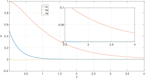
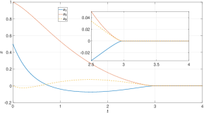
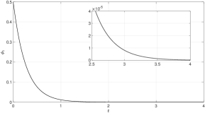
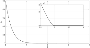
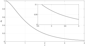
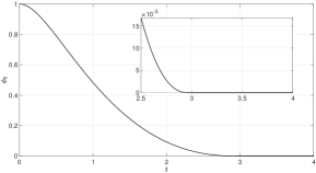
Figure 2: Trajectories of the nominal system (47) with linear (left) and homogeneous (right) nonovershooting stabilizers

6.1 ISS on $\Sigma$

Let us consider the perturbed system

(62) $$\dot{x}=f(x,q):=Ax+Bu(x)+D|qx_{1}|^{\nu},\quad D=\left(\begin{smallmatrix}1\\ 0\\ 0\end{smallmatrix}\right)\quad 0<\nu<1+\mu,$$

where $\mu>-1$, $x=(x_{1},x_{2},x_{3})^{\top}$, $A$, $B$ are as before, $u$ is either a linear or a homogeneous nonovershooting stabilizer and $q\in L^{\infty}(\mathbb{R},\mathbb{R})$ is an uncertain parameter. Since $\mathbf{d}(s)D=e^{s}\sum_{i=0}^{\infty}\tfrac{s^{i}\mu^{i}G_{0}^{i}}{i!}D=e^{s}D$ then taking $\tilde{\mathbf{d}}(s)=e^{\left(\frac{1+\mu}{\nu}-1\right)s}$, for $u$ given by (54), we derive $f(\mathbf{d}(s)x,\tilde{q})=e^{\mu s}\mathbf{d}(s)f(x,q),\forall s\in\mathbb{R},x\in\mathbb{R}^{n},q\in\mathbb{R}.$ The group $\tilde{\mathbf{d}}(s)$ is a dilation in $\mathbb{R}$ if $0<\nu<1+\mu$. Hence, taking into account global asymptotic stability of the system (62) for $q=\mathbf{0}$ we conclude ISS with respect to $q$ on $\mathbb{R}^{n}$. To prove invariance of $\Sigma$ in the perturbed case we check the condition (39) for $p=2$. Since $h_{1}^{\top}G_{\mathbf{d}}x=h_{1}x,\quad h_{2}^{\top}G_{\mathbf{d}}x=(1-\mu)h_{2}^{\top}x$ then (39) is fulfilled for $p=2$ and the closed-loop system is ISS on $\Sigma$ provided that Assumption 4 is fulfilled.

The simulations results for the perturbed case ($q=\sin(5t),\nu=1/8$) are shown on Figure 3. The homogeneous stabilizer demonstrates a better suppression of perturbations (at least for the selected initial condition and the selected perturbation).

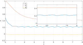
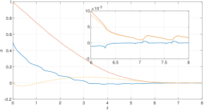
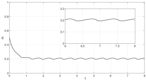
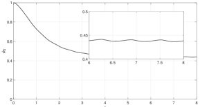
Figure 3: Trajectories of the perturbed system (62) with linear (left) and homogeneous (right) nonovershooting stabilizers

6.2 ISSf on $\Omega$

Let us consider the perturbed system

(63) $$\dot{x}=f(x,q):=Ax+Bu(x+q_{1})+q_{2},$$

where $\mu>-1$, $x=(x_{1},x_{2},x_{3})^{\top}$, $A$, $B$ are as before, $u$ is either a linear or a homogeneous nonovershooting stabilizer designed above and $q=(q_{1}^{\top},q_{2}^{\top})^{\top}\in L^{\infty}(\mathbb{R},\mathbb{R}^{6})$ defines both measurement noise and additive perturbation.

Using the representation (61) we conclude that $-H(A+BK)H^{-1}r\in\mathbb{R}^{n}_{+}$ for $r=(0.2,1,0.2)^{\top}$. So, in the view of Corollary 5.7, the perturbed system (63) is ISSf and ISSfS, at least, for $\mu$ being sufficiently close to zero. The results of numerical simulations for the non-overshooting linear and homogeneous stabilizers designed above are given on Figure 4. The measurement noise $q_{1}$ has been simulated as a uniformly distributed random variable with the magnitude $0.01$. The exogenous perturbation has been defined as follows $q_{2}(t)=\left(1,1,1\right)^{\top}\sin(5t)$.

The simulation results demonstrate faster convergence, better robustness and smaller overshoots of the homogeneous control system comparing with the linear one.

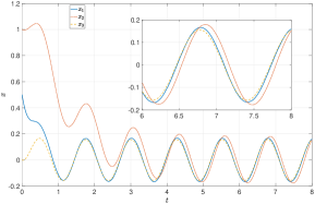
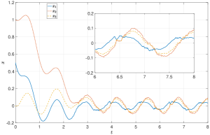
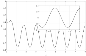
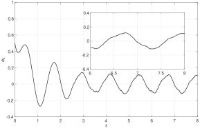
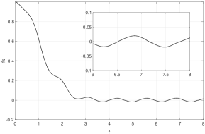
Figure 4: Trajectories of the pertubed system (63) with linear (left) and homogeneous (right) nonovershooting stabilizers

7 Conclusions

In the paper, a scheme for nonovershooting finite-time stabilizer design for linear multi-input system is presented. The procedure is based on an upgrade of a linear nonovershooting stabilizer to a homogeneous one with negative degree. Robustness of the safety and finite-time stability properties is analyzed using the concept of Input-to-State Safety and Input-to-State Stability. For this purpose, some known results about ISS analysis of homogeneous systems in $\mathbb{R}^{n}$ are expanded to homogeneous systems on homogeneous cones. The presented example illustrates the simplicity of the proposed scheme of control design and robustness analysis.

References

- [1] I. Abel, D. Steeves, M. Krstic, and M. Jankovic. Prescribed-time safety design for a chain of integrators. In American Control Conference, 2022.
- [2] A. D. Ames, J. W. Grizzle, and P. Tabuada. Control barrier function based quadratic programs with application to adaptive cruise contro. In Conference on Decision and Control, pages 6271–6278, 2014.
- [3] A. D. Ames, J. W. Grizzle, and P. Tabuada. Ccontrol barrier function based quadratic programs for safety critical systems. IEEE Transactions on Automatic Control, 62:3861–3876, 2017.
- [4] V. Andrieu, L. Praly, and A. Astolfi. Homogeneous Approximation, Recursive Observer Design, and Output Feedback. SIAM Journal of Control and Optimization, 47(4):1814–1850, 2008.
- [5] J.-P. Aubin. Viability theory. Birkhauser, 1991.
- [6] E. Bernuau, A. Polyakov, D. Efimov, and W. Perruquetti. Verification of ISS, iISS and IOSS properties applying weighted homogeneity. System & Control Letters, 62(12):1159–1167, 2013.
- [7] S. P. Bhat and D. S. Bernstein. Geometric homogeneity with applications to finite-time stability. Mathematics of Control, Signals and Systems, 17:101–127, 2005.
- [8] F. Blanchini. Set invariance in control. Automatica, 35:1747–1767, 1999.
- [9] F. Blanchini and S. Miani. Set-Theoretic Methods in Control. Birkhauser, 2016.
- [10] S. Boyd, E. Ghaoui, E. Feron, and V. Balakrishnan. Linear Matrix Inequalities in System and Control Theory. Philadelphia: SIAM, 1994.
- [11] E. A. Coddington and N. Levinson. Theory of Ordinary Differential Equations. New York, McGraw-Hill, 1955.
- [12] S. Darbha and S. P. Bhattacharrya. On the synthesis of controllers for a nonovershooting step response. IEEE Transactions on Automatic Control, 48(5):797–799, 2003.
- [13] P. De Leenheer and D. Aeyels. Stabilization of positive linear systems. Systems & Control Letters, 44:259–271, 2001.
- [14] M. El-Khoury, O. D. Crisall, and R. Longchamp. Influence of zero locations on the number of step-response extre. Automatica, 29:1571–1574, 1993.
- [15] L. Farina and S. Rinaldi. Positive Linear Systems; Theory and Applications. John Wiley, 2000.
- [16] A. F. Filippov. Differential Equations with Discontinuous Right-hand Sides. Kluwer Academic Publishers, 1988.
- [17] V. Fischer and M. Ruzhansky. Quantization on Nilpotent Lie Groups. Springer, 2016.
- [18] K. Garg, R. K. Cosner, U. Rosolia, A. D. Ames, and D. Panagou. Multi-rate control design under input constraints via fixed-time barrier functions. IEEE Control Systems Letters, 6:608–613, 2022.
- [19] L. Grüne. Homogeneous state feedback stabilization of homogeneous systems. SIAM Journal of Control and Optimization, 38(4):1288–1308, 2000.
- [20] Y. Hong. H∞ control, stabilization, and input-output stability of nonlinear systems with homogeneous properties. Automatica, 37(7):819–829, 2001.
- [21] Y. Hong, Z. Jiang, and G. Feng. Finite-time input-to-state stability and applications to finite-time control design. SIAM Journal on Control and Optimization, 48(7):4395–4418, 2010.
- [22] L.S. Husch. Topological Characterization of The Dilation and The Translation in Frechet Spaces. Mathematical Annals, 190:1–5, 1970.
- [23] M. Jankovic. Robust control barrier functions for constrained stabiliza- tion of nonlinear systems. Automatica, 96:359–367, 2018.
- [24] M. Kawski. Families of dilations and asymptotic stability. Analysis of Controlled Dynamical Systems, pages 285–294, 1991.
- [25] V. V. Khomenuk. On systems of ordinary differential equations with generalized homogenous right-hand sides. Izvestia vuzov. Mathematica (in Russian), 3(22):157–164, 1961.
- [26] S. Kolathaya and A. D. Ames. Input-to-state safety with control barrier functions. IEEE Control Systems Letters, 3(1):108 – 113, 2019.
- [27] M. Krstic and M. Bement. Nonovershooting control of strict-feedback nonlinear systems. IEEE Transactions on Automatic Control, 51(12):1938–1943, 2006.
- [28] L. Lindemann and D. V. Dimarogonas. Control barrier functions for multi-agent systems under conflicting local signal temporal logic tasks. IEEE Control Systems Letters, 3(3), 2019.
- [29] L. Magni, D.M. Raimondo, and R. Scattolini. Regional input-to-state stability for nonlinear model predictive control. IEEE Transactions on Automatic Control, 51(9):1548–1553, 2006.
- [30] J. L. Massera. On lyapunovff’s conditions of stability. Annals of Mathematics, 50:705–721, 1949.
- [31] M. Nagumo. Uber die lage der integralkurven gewohnlicher differentialgleichungen. Proceedings of the Physico-Mathematical Society of Japan, 24:551–559, 1942.
- [32] H. Nakamura, Y. Yamashita, and H. Nishitani. Smooth Lyapunov functions for homogeneous differential inclusions. In Proceedings of the 41st SICE Annual Conference, pages 1974–1979, 2002.
- [33] A. Nekhoroshikh, D. Efimov, A. Polyakov, W. Perruquetti, and I. Furtat. Finite-time stabilization under state constraints. In Conference on Decision and Control, 2021.
- [34] A. Pazy. Semigroups of Linear Operators and Applications to Partial Differential Equations. Springer, 1983.
- [35] S. F. Phillips and D. E. Seborg. Conditions that guarantee no overshoot for linear system. International Journal of Control, 47(4):1043–1059, 1988.
- [36] A. Polyakov. Sliding mode control design using canonical homogeneous norm. International Journal of Robust and Nonlinear Control, 29(3):682–701, 2019.
- [37] A. Polyakov. Generalized Homogeneity in Systems and Control. Springer, 2020.
- [38] A. Polyakov. Input-to-State Stability of Homogeneous Infinite Dimensional Systems with Locally Lipschitz Nonlinearities. Automatica, 129:109615, 2021.
- [39] A. Polyakov and M. Krstic. Finite-and fixed-time nonovershooting stabilizers and safety filters by homogeneous feedback. IEEE Transaction on Automatic Control, 2023.
- [40] A. Poznyak, A. Polyakov, and V. Azhmyakov. Attractive Ellipsoids in Robust Control. Birkhauser, 2014.
- [41] Y. Rahman, M. Jankovic, and M. Santill. Driver intent prediction with barrier functions. In American Control Conference, pages 224–230, 2021.
- [42] A. Rantzer. Scalable control of positive systems. European Journal of Control, 24(7):72–80, 2015.
- [43] L. Rosier. Homogeneous Lyapunov function for homogeneous continuous vector field. Systems & Control Letters, 19:467–473, 1992.
- [44] E.P. Ryan. Universal stabilization of a class of nonlinear systems with homogeneous vector fields. Systems & Control Letters, 26:177–184, 1995.
- [45] M. Santillo and M. Jankovic. Collision free navigation with interacting, non-communicating obstacles. In American Control Conference, pages 1637–1643, 2021.
- [46] E.D. Sontag. Smooth stabilization implies coprime factorization. IEEE Transactions on Automatic Control, 34:435–443, 1989.
- [47] E.D. Sontag and Y. Wang. On characterizations of the input-to-state stability property. Systems & Control Letters, 24(5):351–359, 1996.
- [48] E. Soontag and Y. Wang. A notion of input to output stability. In European Control Conference, pages 3862–3867, 1997.
- [49] L. Wang, A.D. Ames, and M. Egerstedt. Safety barrierc ertificates for collisions-free multirobot systems. IEEE Transactions on Robotics, 33(3):661–674, 2017.
- [50] S. Wang, A. Polyakov, and G. Zheng. Generalized homogenization of linear controllers: Theory and experiment. International Journal of Robust and Nonlinear Control, 31(9):3455–3479, 2021.
- [51] P. Wieland and F. Allgöwer. Constructive safety using control barrier functions. In IFAC Proceedings Volumes, volume 40, pages 462–467,, 2007.
- [52] K. Zimenko, A. Polyakov, D. Efimov, and W. Perruquetti. Robust feedback stabilization of linear mimo systems using generalized homogenization. IEEE Transactions on Automatic Control, 2020.
- [53] V.I. Zubov. On systems of ordinary differential equations with generalized homogeneous right-hand sides. Izvestia vuzov. Mathematica (in Russian), 1:80–88, 1958.