A Learning-Inspired Strategy to Design Binary Sequences with Good Correlation Properties: SISO and MIMO Radar Systems

Abstract

In this paper, the design of binary sequences exhibiting low values of aperiodic/periodic correlation functions, in terms of Integrated Sidelobe Level (ISL), is pursued via a learning-inspired method. Specifically, the synthesis of either a single or a burst of codes is addressed, with reference to both Single-Input Single-Output (SISO) and Multiple-Input Multiple-Output (MIMO) radar systems. Two optimization machines, referred to as two-layer and single-layer Binary Sequence Correlation Network (BiSCorN), able to learn actions to design binary sequences with small ISL/Complementary ISL (CISL) for SISO and MIMO systems are proposed. These two networks differ in terms of the capability to synthesize Low-Correlation-Zone (LCZ) sequences and computational cost. Numerical experiments show that proposed techniques can outperform state-of-the-art algorithms for the design of binary sequences and Complementary Sets of Sequences (CSS) in terms of ISL and, interestingly, of Peak Sidelobe Level (PSL).

I Introduction

An active sensing device such as a radar system can determine useful information on the prospective targets by transmitting waveforms toward an intended region and then analyzing the received signal. Transmit waveform is thus a critical factor that can improve the performance of active sensing systems. Indeed, an appropriate selection of the probing signals may lead to a better target detectability as well as a more accurate parameter estimation process [1, 2, 3]. Designing sequences with good correlation properties, i.e., small Integrated Sidelobe Level (ISL)/Peak Sidelobe Level (PSL), has attracted a lot of attention in radar signal processing community since such sequences rule the quality of the pulse compression process. Notably, in modern active sensing and radar systems a special interest is deserved to the design of binary codes due to their implementation simplicity.

The design of binary sequences has been addressed in several works. For example, M-sequences as well as Gold and Kasami codes have good periodic auto-correlation properties [4] ensuring optimal performance under certain conditions, e.g., M-sequences are only available for specific length $2^{N-1}$. Another important instance is represented by the Barker codes that are unfortunately limited to a finite length of 13. The authors in [5, 6, 7] extended the Barker sequences by some heuristic algorithms to propose generalized poly-phase Barker sequences. The mentioned works are also limited to length 77 [8]. [9] proposed a cyclic algorithm to design in a computationally efficient way constant modulus sequence with small ISL (see [10] for a related paper to design binary codes). In [11] the ISL minimization problem was addressed by means of Majorization-Minimization (MM) technique. This MM-based algorithm can be faster than procedure proposed in [9] under some conditions. Moreover, the authors of [12] consider the problem of sequence design with good correlation properties, in terms of ISL and PSL, for sequences with either continuous or discrete phases. The optimization problem in the aforementioned reference was tackled by an iterative algorithm based on Coordinate-Descent (CD) optimization.

Another important line of studies focuses on the Multiple-Input Multiple-Output (MIMO) radar systems which can offer improved target detection and recognition performance. MIMO radars often rely on almost orthogonal sets of sequences with good auto- and cross-correlation properties. Therefore, the design of waveforms with small ISL of the auto- and cross- correlations for MIMO radar systems has been pursued in a plethora of works. Among them, it is worth mentioning Multi-CAN [13], MM-Corr [14], ISLNew [15, 16], Iterative Direct Search [17], Doppler resilient complete complementary codes [18], and consensus-ADMM/PDMM [19] algorithms. All of the aforementioned procedures almost meet the lower bound on ISL for sets of sequences with continuous phases [20]. The BiST algorithm [21] extends the previous works to design sets of binary sequences with good correlation properties for MIMO radar systems.

An idea to improve the correlation properties of a sequence is increasing the degrees of freedom at the design stage. To achieve this goal, some researchers consider Complementary Sets of Sequences (CSS) where multiple codes are transmitted instead of a single one. Most of the studies concerning CSS have been focused on the generation in closed-form of CSS and involve restrictions on the sequence length and set cardinality. However, an efficient computational method was introduced in [22]. Among others, some low complexity procedures were devised e.g., CANARY [23], MM-CSS [14], QOZCP [24], and Bare MM-CSS, MM-CSS-SQUARE, MM-CSS-SD algorithms [25].

Recently, machine learning approaches have been employed to address various engineering problems like computer vision [26], watermarking [27], low-resolution receiver design [28], and UAV navigation [29]. Particularly, machine learning is used for waveform design and power allocation in communication systems [30, 31]. This emerging paradigm has provided successful solution to the aforementioned problems. Therefore, we consider learning approaches for radar sequence design, a promising research area deserving special attention.

In light of above discussions, in this paper we devise two learning-inspired frameworks to deal with the synthesis of binary sequences with good correlation properties. The proposed design methodologies, referred to as, two-layer and single-layer Binary Sequence Correlation Network (BiSCorN), exploit neural network tools to tackle sequence design problems. The design problems are formulated in terms of Weighted ISL (WISL) minimization for various radar system setups/models, including Single-Input Single-Output (SISO), MIMO, CSS, MIMO-CSS, and subject to a constraint imposing binary elements. All the resulting code optimization problems are handled under a unified mathematical umbrella offered by BiSCorN. Specially, single-layer and two-layer BiSCorN are employed to deal with the design problems; these two methods are different in terms of the capability to design Low-Correlation-Zone (LCZ) sequences and computational complexity (to be discussed shortly). Note that the proposed method is not a conventional learning method as it is common in the literature; however, it is a learning method, since discover how probing the environment by a training phase. Therefore, the main contributions of the work can be summarized as: (i) developing the theoretical background for learning-inspired sequence design and (ii) devising a network architecture as well as a network feeding approach for the exploitation of the ADAM algorithm. At the analysis stage, numerical experiments are reported to show the effectiveness of the proposed BiSCorN also in comparison with the state-of-the-art methods. Note that a limited part of this work has been presented in [32]; more precisely, the aforementioned conference article addressed only SISO systems without mathematical backgrounds.

The rest of this paper is organized as follows. In Section II the design problems related to the different system setups are formulated and then, two-layer BiSCorN is developed to deal with the aforementioned design problems. In Section III, the single-layer BiSCorN is proposed to design LCZ sequences for all considered system setups. The implementation process as well as computational complexity are discussed in Section IV. The performance of the proposed techniques is assessed in Section V. Finally, the conclusions are drawn in Section VI, followed by possible future research lines.

Notation: Bold lowercase letters and bold uppercase letters are used for vectors and matrices respectively. The $l_{2}$-norm of a vector ${\bf x}$ and Frobenius norm of a matrix ${\bf X}$ are denoted by $\|{\bf x}\|_{2}$ and $\|{\bf X}\|_{F}$, respectively. $\mathbb{R}^{N\times N}$ ($\mathbb{R}^{N}$) indicates the set of ${N\times N}$ (${N\times 1}$) real matrices (column vectors). $\mathbb{R}^{N}_{+}$ represents set of (${N\times 1}$) vectors with non-negative real entries. The absolute value of the scalar $x$ is denoted by $|x|$, whereas ${(\cdot)^{{T}}}$ indicates the transpose operator. $\mathbb{E}_{{\bf x}}[\cdot]$ stands for the statistical expectation with respect to (w.r.t.) ${\bf x}$. $\lfloor x\rfloor$ is the greatest integer less than or equal to $x$ and $\lceil x\rceil$ is the least integer greater than or equal to $x$. $\mathcal{N}(\bm{\omega},\mathbf{\Sigma})$ denotes a Gaussian distribution with mean $\bm{\omega}$ and covariance matrix $\mathbf{\Sigma}$. ${x}_{\textrm{\tiny{mod}}\hskip 1.0pty}$ is equal to $x-\lfloor\frac{x}{y}\rfloor y$ for $x\in\mathbb{R}$ and $y\in\mathbb{R}_{+}$. The notation ${\nabla}_{{\mathbf{x}}}f(\cdot)$ indicates the gradient of a function w.r.t. $\mathbf{x}$. $\textrm{Diag}(\mathbf{x})$ denotes the diagonal matrix formed by the entries of the vector argument $\mathbf{x}$. $\mathbf{I}_{N}\in\mathbb{R}^{N\times N}$ represents the identity matrix and $\mathbf{e}_{n}\in\mathbb{R}^{N}$ is the $n^{th}$ standard vector. Bold numbers $\mathbf{1}$ and $\mathbf{0}$ are for vectors whose elements are all one and all zero, respectively.

II Problem Formulation and the Proposed BiSCorN

In this section, first, a SISO system is considered and a learning-based network, referred to as two-layer BiSCorN, is proposed for designing binary sequences with small periodic/aperiodic WISL. Then, the proposed approach is extended to MIMO systems. Finally, BiSCorN is modified to design binary complementary sequences with small Weighted Complementary ISL (WCISL) in (either SISO or MIMO) systems.

II-A SISO

Let us define $\mathbf{x}=[x(1),x(2),...,x(N)]^{T}\in\mathbb{R}^{N}$ as a transmit fast-time SISO radar sequence with length $N$. The aperiodic and periodic auto-correlation functions of $\mathbf{x}$ can be defined as

$$r_{AP}(k)=\sum_{n=1}^{N-k}x(n)\hskip 1.0ptx(n+k),~{}~{}~{}k=0,...,N-1,$$ (1)

and

$$r_{P}(k)=\sum_{n=1}^{N}x(n)\hskip 1.0ptx{({(n+k)}_{\textrm{\tiny{mod}}\hskip 1.0ptN})},~{}~{}~{}k=0,...,N-1,$$ (2)

respectively. Note that in the definitions above, $r_{AP}(0)$ and $r_{P}(0)$ coincide with the energy of the sequence $\mathbf{x}$, while all the other aperiodic/periodic auto-correlation values, i.e., $\{r_{AP}(k)|^{N-1}_{k=1}\}$ and $\{r_{P}(k)|^{N-1}_{k=1}\}$, are referred to as sidelobes [1].

In the following, WISL is considered as the design metric to measure the quality of sequences in terms of correlation properties. Precisely, letting $\mathbf{w}_{\mathcal{S}}=[w_{\mathcal{S},1},w_{\mathcal{S},2},...,w_{\mathcal{S},N-1}]^{T}$ with $w_{\mathcal{S},k}\geq 0,\hskip 2.0ptk=1,...,N-1,$ the WISL for the SISO case can be defined as:

$$\textrm{WISL}=2\sum_{k=1}^{N-1}w_{\mathcal{S},k}|r(k)|^{2},$$ (3)

where, with a slight abuse of notation, $r(k)$ refers to either $r_{AP}(k)$ or $r_{P}(k)$, depending on the specific design instance. Note that the special case of ISL can be obtained by selecting $\mathbf{w}_{\mathcal{S}}=\mathbf{1}$. Hence, the synthesis of binary sequences for SISO systems can be formulated as

$$\min_{\mathbf{x}} \displaystyle\sum_{k=1}^{N-1}w_{\mathcal{S},k}|r(k)|^{2}$$ (4)

s. t. $$x(n)\in\{-1,+1\},~{}~{}n=1,...,N,$$

which is a non-convex NP-hard optimization problem [9].

In the sequel, a learning-based network is proposed to deal with the minimization problem in (4). We start with a relaxation of the binary constraint on the code elements in (4). Precisely, we allow the elements of the code vary within $[-1,1]$. Since $\mathbf{x}=\mathbf{0}$ is the trivial solution to the relaxed problem, the term $w_{\mathcal{S},b}|r(0)-N|^{2}$ is added to the objective function. Therefore, the solution present a value of $r(0)$ closer and closer to $N$ as ${w}_{\mathcal{S},b}$ approaches one avoiding the trivial solution. This trick leads to the following reformulated version of (4):

$$\min_{\mathbf{x}} \widetilde{\mathbf{w}}^{T}_{\mathcal{S}}\hskip 1.0pt\hskip 1.0pt\widetilde{\mathbf{r}}_{\mathcal{S}}$$ (5)

s. t. $$|x(n)|\leq 1,~{}~{}n=1,...,N,$$

where $\widetilde{\mathbf{w}}_{\mathcal{S}}=[w_{\mathcal{S},b},w_{\mathcal{S},s}\times\mathbf{w}^{T}_{\mathcal{S}}]^{T}\in\mathbb{R}^{N}_{+}$ with $w_{\mathcal{S},b}+w_{\mathcal{S},s}=1,\hskip 2.0ptw_{\mathcal{S},b}\geq 0,\hskip 2.0ptw_{\mathcal{S},s}\geq 0$ and

$$\widetilde{{r}}_{\mathcal{S}}(k)=\begin{cases}|r(0)-N|^{2},~{}~{}k=1,\\ |r(k)|^{2},~{}~{}~{}~{}~{}~{}~{}k=2,...,N.\end{cases}$$ (6)

This trick also paves the way to partially manage the synthesis loss, viz. the loss/degradation in the objective function of (4) required to obtain feasible binary elements for the codes from the solution to the reformulated version (see Remark 1 for details). Specifically, being $|x(n)|\leq 1$ it follows that $r(0)=\sum_{n=1}^{N}|x(n)|^{2}\leq N$. Thus, decreasing the term $|r(0)-N|^{2}$ leads to $|x(n)|$ approaching one for any $n$, i.e., near binary solutions for the real-valued variables. In light of above discussion, one can conclude that the parameters $w_{\mathcal{S},b}$ and $w_{\mathcal{S},s}$ can be used to manage binarization and sidelobe level: increasing $w_{\mathcal{S},b}$ makes the sequence closer to the binary solution and increasing $w_{\mathcal{S},s}$ gives more emphasis on the sidelobe terms. The following lemma sheds light on the theoretical connections between Problems (4) and (5).

Lemma 1.

Let $\mathcal{P}^{(i)}$, $i\geq 1$, be the optimization problem in (5) with $w_{\mathcal{S},b}^{(i)}=\frac{\bar{w}_{\mathcal{S},b}^{(i)}}{\bar{w}_{\mathcal{S},s}+\bar{w}_{\mathcal{S},b}^{(i)}}$ and $w_{\mathcal{S},s}^{(i)}=\frac{\bar{w}_{\mathcal{S},s}}{\bar{w}_{\mathcal{S},s}+\bar{w}_{\mathcal{S},b}^{(i)}}$, where ${\bar{w}_{\mathcal{S},b}^{{(i)}}}>0$, $i\geq 1$, while $\bar{w}_{\mathcal{S},s}>0$ is fixed. Now, denoting by $\mathbf{x}^{(i)}$ an optimal solution to Problem $\mathcal{P}^{(i)}$, $i\geq 1$, if $\bar{w}_{\mathcal{S},b}^{(i)}\rightarrow\infty$ as $i\,\to\,+\infty$, it follows that

• for any $n=1,...,N$, $\left|x^{(i)}(n)\right|\,\to\,1$ as $i\,\to\,+\infty$;

• any cluster point to the generated sequence $\mathbf{x}^{(i)}$ is an optimal solution to the original problem in (4).

Proof: See Appendix A. $\hskip 325.0pt\blacksquare$ According to Lemma 1, we can deal with the optimization problem in (4) by considering the modified design in (5); in particular, it is possible by either supposing a sequence of design problems $\mathcal{P}^{(i)}$ e.g., with $\bar{w}_{\mathcal{S},b}^{(i)}$ proportional to $2^{(i-1)}$, $i\geq 1$, or employing a practically fixed large enough $\bar{w}_{\mathcal{S},b}^{(i)}$. Indeed, by solving Problem (5) for increasing values of ${w}_{\mathcal{S},b}$, an optimal solution to (4) can be asymptotically achieved.

We begin the code design for SISO case via a learning-based framework. Indeed, the objective function of Problem (5) can be considered as the loss function of a neural network in which the desired solution is not the network output but the network weights, as opposed to the typical usages of neural networks in the literature [26, 27]. Precisely, we propose a two-layer fully connected BiSCorN with the following loss function

$$\mathcal{L}_{\mathcal{S}} =\left\|\mathbf{y}_{\mathcal{S}}\left(\mathbf{s}_{\mathcal{S}},\mathbf{x}\right)-N\mathbf{s}_{\mathcal{S}}\right\|_{2}^{2},$$ (7)

where ${\mathbf{s}_{\mathcal{S}}}\in\mathbb{R}^{N}$ is the network input, $N\hskip 1.0pt\mathbf{s}_{\mathcal{S}}$ is the desired output, and $\mathbf{y}_{\mathcal{S}}$ is the output of the network. As shown in Fig. 1.a, the output vector can be obtained as $\mathbf{y}_{\mathcal{S}}\left(\mathbf{s}_{\mathcal{S}},\mathbf{x}\right)=\mathbf{X}^{T}_{\mathcal{S}}\mathbf{X}_{\mathcal{S}}\mathbf{s}_{\mathcal{S}}$, where the matrix $\mathbf{X}_{\mathcal{S}}$ and its transpose can be used respectively for the first and second layer weights of the BiSCorN. For notation simplicity, $\mathbf{X}_{\mathcal{S}}$ denotes either $\mathbf{X}_{\mathcal{S},P}$ or $\mathbf{X}_{\mathcal{S},AP}$, i.e.,

$$\mathbf{X}_{\mathcal{S}}(\mathbf{x})=\begin{cases}\mathbf{X}_{\mathcal{S},AP}(\mathbf{x}),\hskip 8.0pt\textrm{Aperiodic},\\ \mathbf{X}_{\mathcal{S},P}(\mathbf{x}),\hskip 15.0pt\textrm{Periodic},\end{cases}$$ (8)

where

$$\mathbf{X}_{\mathcal{S},P}(\mathbf{x})=[\mathbf{x}_{P,0}(\mathbf{x}),\mathbf{x}_{P,1}(\mathbf{x}),...,\mathbf{x}_{P,N-1}(\mathbf{x})]\in\mathbb{R}^{N\times N},$$ (9)

$$\mathbf{X}_{\mathcal{S},AP}(\mathbf{x})=[\mathbf{x}_{AP,0}(\mathbf{x}),\mathbf{x}_{AP,1}(\mathbf{x}),...,\mathbf{x}_{AP,N-1}(\mathbf{x})]\in\mathbb{R}^{(2N-1)\times N},$$ (10)

with $\mathbf{x}_{P,i}(\mathbf{x})$ and $\mathbf{x}_{AP,i}(\mathbf{x})$ are respectively the circularly shifted versions of $\mathbf{x}$ and $\mathbf{x}_{\textrm{pad}}=[\mathbf{x}^{T},0,0,...,0]^{T}$ $\in\mathbb{R}^{2N-1}$ by $i$ elements (as shown in Fig. 1.b). Note that the constraint $|x(n)|\leq 1,~{}n=1,...,N-1,$ is applied to the network weights (see [35] for a similar case).

Figure 1: Two-layer BiSCorN to design aperiodoc/periodic binary sequences within the SISO radar context.

Then, by substituting $\mathbf{X}_{\mathcal{S}}$, the $k^{th}$ entry of the network output can be written as (see Appendix B)

$$y_{\mathcal{S},k}=\begin{cases}\sum_{i=1}^{N}r(i-1)\hskip 2.0pts_{\mathcal{S},i},\hskip 113.0ptk=1,\\ \sum_{i=1}^{k}r(k-i)\hskip 2.0pts_{\mathcal{S},i}+\sum_{i=k+1}^{N}r(i-k)\hskip 2.0pts_{\mathcal{S},i},\hskip 8.0pt2\leq k\leq N-1,\\ \sum_{i=1}^{N}r(N-i)\hskip 2.0pts_{\mathcal{S},i},\hskip 108.0ptk=N.\end{cases}$$ (11)

Herein, by selecting $\mathbf{s}_{\mathcal{S}}=[{a_{\mathcal{S}}},0,0,...,0]^{T}\in\mathbb{R}^{N}$ (for arbitrary $a_{\mathcal{S}}\neq 0$) and by using (6) as well as (11), the loss function in (7) boils down to

$$\mathcal{L}_{\mathcal{S}} =a^{2}_{\mathcal{S}}\left((r(0)-N)^{2}+r^{2}(1)+...+r^{2}(N-1)\right)=\mathbf{a}^{T}_{\mathcal{S}}\hskip 2.0pt\widetilde{\mathbf{r}}_{\mathcal{S}},$$ (12)

where $\mathbf{a}_{\mathcal{S}}=[a^{2}_{\mathcal{S}},a^{2}_{\mathcal{S}},...,a^{2}_{\mathcal{S}}]^{T}\in\mathbb{R}^{N}_{+}$. Accordingly, the architecture in Fig. 1 can deal with the design problem in (5) as long as equal ISL weights are considered, i.e., $\widetilde{\mathbf{w}}_{\mathcal{S}}=\mathbf{a}_{\mathcal{S}}$. Note that the equal weights do not necessarily lead to optimal binary solutions as addressed by Lemma 1; however, we numerically observed that binary sequences associated with the equal weights possess good correlation properties (see Remark 1 below and Section V). Furthermore, another version of BiSCorN accounting for arbitrary weights and hence those addressed in Lemma 1 will be devised in Section III.

Remark 1 (synthesis stage).

The feasible set of the design problem in (4) for the special case of $N=3$ consists of vertices of a cube centered at origin with the side length equal to 2. Whereas, for the relaxed problem in (5), the feasible set is the total volume inside the aforementioned cube. Note that the objective function in Problem (5) includes a penalty term for non-binary solutions (that is, deviation from the vertices of the cube). However, the proposed method might converge to sequences with a few non-binary elements (see Subsection V-A2). For example, Fig. 2 shows a solution for the relaxed problem that is located at one of the cube edges: having two binary elements and one non-binary element. Therefore, a final stage is used after convergence of the method to quantize non-binary elements to the nearest values in the set $\{-1,+1\}$ and obtain a feasible sequence to the original design problem in (4).

Figure 2: The feasible set of the SISO problem in (5) for $N=3$.

Remark 2 (another perspective on BiSCorN).

It is known that the transmitted binary sequence $\mathbf{x}$ has ideal auto-correlation properties if $r(0)=N$ and $r(k)=0,~{}k=1,...,N-1$. Therefore, for an ideal sequence design scheme $\mathbf{X}^{T}_{\mathcal{S}}\mathbf{X}_{\mathcal{S}}=N\mathbf{I}_{N}$. We expect that exploiting BiSCorN provides a matrix $\mathbf{X}_{\mathcal{S}}$ such that $\mathbf{X}^{T}_{\mathcal{S}}\mathbf{X}_{\mathcal{S}}\approx N\mathbf{I}_{N}$. To evaluate the performance of BiSCorN, one may define $\mathbf{E}=\frac{1}{N}\mathbf{X}^{T}_{\mathcal{S}}\mathbf{X}_{\mathcal{S}}$; and next feed the network with a random test signal for monitoring the entries of $\mathbf{E}$ (see Section IV for more details). That is, the lower the energy of off-diagonal entries the better the performance. The evaluation of the normalized loss function, i.e., $\frac{\mathcal{L}_{\mathcal{S}}}{N}$, for $10$ random input signals (as test signals) before and after quantization are shown in Fig. 3.a for the case of $N=50$. Also, Fig. 3.b-c exemplify the matrix $\mathbf{E}$ in a grayscale image and its corresponding network input/output are shown for a trial in Fig. 3.d-e. Precisely, Fig. 3.d-e show that how closely the network output follows the network input. This figure illustrates the goodness of BiSCorN even after applying quantization.

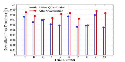
(a) Normalized evaluated loss function for 10 trials.

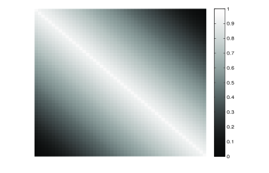
(b) The grayscale image of matrix $\mathbf{E}=\frac{1}{N}\mathbf{X}^{T}_{\mathcal{S}}\mathbf{X}_{\mathcal{S}}$ before quantization.

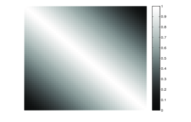
(c) The grayscale image of matrix $\mathbf{E}=\frac{1}{N}\mathbf{X}^{T}_{\mathcal{S}}\mathbf{X}_{\mathcal{S}}$ after quantization.

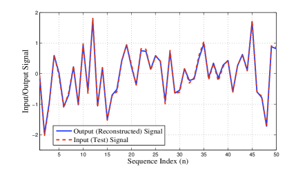
(d) Amplitude of input/output signals before quantization.

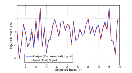
(e) Amplitude of input/output signals after quantization.

Figure 3: Performance evaluation of SISO two-layer BiSCorN for (test) random input signals before/after quantization for sequence length $N=50$.

II-B MIMO

A MIMO radar equipped with $N_{T}$ transmit antennas is considered, where each antenna emits a different code vector with $N$ subpulses. Let us denote by $\mathbf{x}_{m}=[x_{m}(1),x_{m}(2),...,x_{m}(N)]^{T}\in\mathbb{R}^{N},~{}m=1,...,N_{T},$ the transmit code vector at the $m^{th}$ antenna. The aperiodic and periodic cross-correlation functions between $\mathbf{x}_{m}$ and $\mathbf{x}_{l}$ in MIMO system are defined as

$$r_{AP,ml}(k)=\sum_{n=1}^{N-k}x_{m}(n)\hskip 1.0ptx_{l}(n+k),~{}~{}m,l=1,...,N_{T},~{}~{}-N+1\leq k\leq N-1,$$ (13)

and

$$r_{P,ml}(k)=\sum_{n=1}^{N}x_{m}(n)\hskip 1.0ptx_{l}{({(n+k)}_{\textrm{\tiny{mod}}\hskip 1.0ptN})},~{}~{}m,l=1,...,N_{T},~{}~{}-N+1\leq k\leq N-1,$$ (14)

respectively. Defining $\widetilde{\mathbf{X}}_{\mathcal{M}}=[\mathbf{x}_{1},\mathbf{x}_{2},...,\mathbf{x}_{N_{T}}]$, the design of binary space-time radar codes can be cast as

$$\min_{\widetilde{\mathbf{X}}_{\mathcal{M}}} w_{\mathcal{M},0}\sum_{\begin{subarray}{c}m,l=1\\ m\neq l\end{subarray}}^{N_{T}}|r_{ml}(0)|^{2}+\sum_{k=1}^{N-1}w_{\mathcal{M},k}\sum_{m,l=1}^{N_{T}}|r_{ml}(k)|^{2}+\sum_{k=-N+1}^{-1}w_{\mathcal{M},-k}\sum_{m,l=1}^{N_{T}}|r_{ml}(k)|^{2}$$ (15)

s. t. $$x_{m}(n)\in\{-1,+1\},~{}m=1,...,N_{T},~{}n=1,...,N,$$

where $\mathbf{w}_{\mathcal{M}}=[w_{\mathcal{M},0},w_{\mathcal{M},1},...,w_{\mathcal{M},N-1}]^{T}$ with $w_{\mathcal{M},k}\geq 0,\hskip 2.0ptk=1,...,N-1,$ is the weighting vector associated with the correlation terms and $r_{ml}(k)$ refers to either $r_{AP,ml}(k)$ or $r_{P,ml}(k)$. Note that Problem (15) is a non-convex NP-hard problem [9].

Using the symmetry property $r_{ml}(k)=r_{lm}(-k),\hskip 2.0pt\forall m,l,k$, the objective of (15) can be cast as

$$w_{\mathcal{M},0}\sum_{\begin{subarray}{c}m,l=1\\ m\neq l\end{subarray}}^{N_{T}}|r_{ml}(0)|^{2}+2\sum_{k=1}^{N-1}w_{\mathcal{M},k}\sum_{m,l=1}^{N_{T}}|r_{ml}(k)|^{2}.$$ (16)

Next, similar to the procedures in Subsection II-A, the binary constraint on $x_{m}(n)$ is relaxed in $|x_{m}(n)|\leq 1$ and the term ${w}_{\mathcal{M},b}\sum_{m=1}^{N_{T}}|r_{mm}(0)-N|^{2}$ is added to the objective function to penalize non-binary solutions. Precisely, the design problem in (15) is approximated as

$$\min_{\widetilde{\mathbf{X}}_{\mathcal{M}}} \widetilde{\mathbf{w}}^{T}_{\mathcal{M}}\hskip 1.0pt\hskip 1.0pt\widetilde{\mathbf{r}}_{\mathcal{M}}$$ (17)

s. t. $$|x_{m}(n)|\leq 1,~{}~{}m=1,...,N_{T},~{}~{}n=1,...,N,$$

where

$$\widetilde{{r}}_{\mathcal{M}}(k)=\begin{cases}\sum_{m=1}^{N_{T}}|r_{mm}(0)-N|^{2},\hskip 2.0pt~{}~{}k=1,\\ \sum_{\begin{subarray}{c}m,l=1\\ m\neq l\end{subarray}}^{N_{T}}|r_{ml}(0)|^{2},\hskip 2.0pt~{}~{}~{}~{}~{}~{}~{}\hskip 1.0ptk=2,\\ 2\sum_{m,l=1}^{N_{T}}|r_{ml}(k-1)|^{2},\hskip 2.0pt~{}k=3,...,N+1,\end{cases}$$ (18)

and $\widetilde{\mathbf{w}}_{\mathcal{M}}=[{w}_{\mathcal{M},b},{w}_{\mathcal{M},s}\times\mathbf{w}^{T}_{\mathcal{M}}]^{T}\in\mathbb{R}^{N+1}_{+}$ is the design parameter managing the sidelobe level suppression and amplitude variability of the synthesized code.

To proceed further, let

$$\mathbf{X}_{\mathcal{M}}=\begin{cases}\mathbf{X}_{\mathcal{M},AP}=[\widetilde{\mathbf{X}}_{\mathcal{S},AP}(\mathbf{x}_{1}),\widetilde{\mathbf{X}}_{\mathcal{S},AP}(\mathbf{x}_{2}),...,\widetilde{\mathbf{X}}_{\mathcal{S},AP}(\mathbf{x}_{N_{T}})]~{}\in\mathbb{R}^{(2N-1)\times NN_{T}},\hskip 8.0pt\textrm{Aperiodic},\\ \mathbf{X}_{\mathcal{M},P}=[\widetilde{\mathbf{X}}_{\mathcal{S},P}(\mathbf{x}_{1}),\widetilde{\mathbf{X}}_{\mathcal{S},P}(\mathbf{x}_{2}),...,\widetilde{\mathbf{X}}_{\mathcal{S},P}(\mathbf{x}_{N_{T}})]~{}\in\mathbb{R}^{N\times NN_{T}},\hskip 56.0pt\textrm{Periodic},\end{cases}$$ (19)

where

$$\widetilde{\mathbf{X}}_{\mathcal{S},AP}(\mathbf{x}_{m})=[\mathbf{x}_{AP,0}(\mathbf{x}_{m}),\sqrt{2}\hskip 2.0pt\mathbf{x}_{AP,1}(\mathbf{x}_{m}),...,\sqrt{2}\hskip 2.0pt\mathbf{x}_{AP,N-1}(\mathbf{x}_{m})]\in\mathbb{R}^{(2N-1)\times N},$$ (20)

$$\widetilde{\mathbf{X}}_{\mathcal{S},P}(\mathbf{x}_{m})=[\mathbf{x}_{P,0}(\mathbf{x}_{m}),\sqrt{2}\hskip 2.0pt\mathbf{x}_{P,1}(\mathbf{x}_{m}),...,\sqrt{2}\hskip 2.0pt\mathbf{x}_{P,N-1}(\mathbf{x}_{m})]\in\mathbb{R}^{N\times N},$$ (21)

with $\mathbf{x}_{P,i}(\mathbf{x}_{m})$ and $\mathbf{x}_{AP,i}(\mathbf{x}_{m})$ are defined in Subsection II-A. Then, let us define $\widetilde{\mathbf{X}}_{\mathcal{S}}$ to get either $\widetilde{\mathbf{X}}_{\mathcal{S},AP}$ or $\widetilde{\mathbf{X}}_{\mathcal{S},P}$. In this case, the loss function can be defined as

$$\mathcal{L}_{\mathcal{M}} =\left\|\mathbf{Y}_{\mathcal{M}}\left(\mathbf{S}_{\mathcal{M}},\widetilde{\mathbf{X}}_{\mathcal{M}}\right)-N\mathbf{S}_{\mathcal{M}}\right\|_{F}^{2},$$ (22)

where $\mathbf{S}_{\mathcal{M}}\in\mathbb{R}^{NN_{T}\times N_{T}}$ is the input matrix, $N\mathbf{S}_{\mathcal{M}}$ is the desired output and ${\mathbf{Y}}_{\mathcal{M}}=\mathbf{X}_{\mathcal{M}}^{T}\mathbf{X}_{\mathcal{M}}\hskip 1.0pt\mathbf{S}_{\mathcal{M}}$ is the output of the MIMO two-layer BiSCorN (as shown in Fig. 4). Let us select the input matrix $\mathbf{S}_{\mathcal{M}}$ as the following signal

$$\mathbf{S}_{\mathcal{M}}={a_{\mathcal{M}}}\left[\mathbf{e}_{1},\mathbf{e}_{N+1},...,\mathbf{e}_{(N_{T}-1)N+1}\right]\in\mathbb{R}^{NN_{T}\times N_{T}},$$ (23)

where $\mathbf{e}_{m}\in\mathbb{R}^{NN_{T}}$ is the $m^{th}$ standard vector and $a_{\mathcal{M}}\neq 0$. By using (18), (19), and (23), the loss function in (22) can be rewritten as (see Appendix C)

$$\mathcal{L}_{\mathcal{M}} =a^{2}_{\mathcal{M}}\left(\sum_{m=1}^{N_{T}}|r_{mm}(0)-N|^{2}+\sum_{\begin{subarray}{c}m,l=1\\ m\neq l\end{subarray}}^{N_{T}}|r_{ml}(0)|^{2}+2\sum_{k=1}^{N-1}\sum_{m,l=1}^{N_{T}}|r_{ml}(k)|^{2}\right)=\mathbf{a}^{T}_{\mathcal{M}}\hskip 1.0pt\widetilde{\mathbf{r}}_{\mathcal{M}},$$ (24)

where $\mathbf{a}_{\mathcal{M}}=[{a}^{2}_{\mathcal{M}},{a}^{2}_{\mathcal{M}},...,{a}^{2}_{\mathcal{M}}]^{T}\in\mathbb{R}^{N+1}_{+}$. Evidently, the loss function in (24) corresponds to (17) provided that $\widetilde{\mathbf{w}}_{\mathcal{M}}=\mathbf{a}_{\mathcal{M}}$.

Figure 4: Two-layer BiSCorN to design aperiodoc/periodic binary sequence sets within MIMO radar context.

II-C CSS

This subsection refers to a system where $M$ sequences, i.e., ${\mathbf{x}}_{m^{\prime}}=[{x}_{m^{\prime}}(1),{x}_{m^{\prime}}(2),...,$ ${x}_{m^{\prime}}(N)]^{T}\in\mathbb{R}^{N},~{}m^{\prime}=1,..,M$, are transmitted sequentially in time domain. Let $r_{m^{\prime}}(k)$ be the auto-correlation function of ${\mathbf{x}}_{m^{\prime}}$. At the receive side, $\sum_{m^{\prime}=1}^{M}r_{m^{\prime}}(k)$ is employed for detection purposes (see [23] for more details). In this context, the set $\widetilde{\mathbf{X}}_{\mathcal{C}}=[{\mathbf{x}}_{1},{\mathbf{x}}_{2},...,{\mathbf{x}}_{M}]\in\mathbb{R}^{N\times M}$ is called complementary iff the following condition is satisfied [23]

$$\sum_{m^{\prime}=1}^{M}r_{m^{\prime}}(k)=0,~{}~{}1\leq|k|\leq N-1.$$ (25)

Then, letting $\mathbf{w}_{\mathcal{C}}=[{w}_{\mathcal{C},1},$ ${w}_{\mathcal{C},2},...,{w}_{\mathcal{C},N-1}]^{T}$ with ${w}_{\mathcal{C},k}\geq 0,\hskip 2.0ptk=1,...,N-1,$ the WCISL given by

$$\textrm{WCISL}=2\sum_{k=1}^{N-1}{w}_{\mathcal{C},k}\left|\sum_{m^{\prime}=1}^{M}r_{m^{\prime}}(k)\right|^{2},$$ (26)

can be used to measure the complementarity level of a set of codes. In this case, the design problem for binary sequence sets can be cast as

$$\min_{\widetilde{\mathbf{X}}_{\mathcal{C}}} \displaystyle\sum_{k=1}^{N-1}{w}_{\mathcal{C},k}\left|\sum_{m^{\prime}=1}^{M}r_{m^{\prime}}(k)\right|^{2}$$ (27)

s. t. $$x_{m^{\prime}}(n)\in\{-1,+1\},~{}{m^{\prime}}=1,...,M,~{}n=1,...,N,$$

which is still a non-convex NP-hard optimization problem [23].

Following a line of reasoning similar to those pursued in Subsections II-A and II-B, yields the following reformulated version of (27):

$$\min_{\{\mathbf{x}_{m^{\prime}}\}^{M}_{{m^{\prime}}=1}} \widetilde{\mathbf{w}}^{T}_{\mathcal{C}}\hskip 1.0pt\hskip 1.0pt\widetilde{\mathbf{r}}_{\mathcal{C}}$$ (28)

s. t. $$|x_{m^{\prime}}(n)|\leq 1,~{}~{}{m^{\prime}}=1,...,M,~{}~{}n=1,...,N,$$

where $\widetilde{\mathbf{w}}_{\mathcal{C}}=[{w}_{\mathcal{C},b},{w}_{\mathcal{C},s}\times\mathbf{w}^{T}_{\mathcal{C}}]^{T}\in\mathbb{R}^{N}_{+}$ with ${w}_{\mathcal{C},b}+{w}_{\mathcal{C},s}=1,\hskip 2.0pt{w}_{\mathcal{C},b}\geq 0,\hskip 2.0pt{w}_{\mathcal{C},s}\geq 0$ and

$$\widetilde{{r}}_{\mathcal{C}}(k)=\begin{cases}\left|\sum_{m^{\prime}=1}^{M}r_{m^{\prime}}(0)-MN\right|^{2},~{}~{}k=1,\\ \left|\sum_{m^{\prime}=1}^{M}r_{m^{\prime}}(k)\right|^{2},~{}~{}~{}~{}~{}~{}~{}~{}~{}~{}k=2,...,N.\end{cases}$$ (29)

Hence, we devise BiSCorN framework to deal with (28). In fact, let us denote

$$\mathbf{X}_{\mathcal{C}}=\begin{cases}\mathbf{X}_{\mathcal{C},AP}=[\mathbf{X}^{T}_{\mathcal{S},AP}(\mathbf{x}_{1}),\mathbf{X}^{T}_{\mathcal{S},AP}(\mathbf{x}_{2}),...,\mathbf{X}^{T}_{\mathcal{S},AP}(\mathbf{x}_{M})]^{T}~{}\in\mathbb{R}^{(2N-1)M\times N},\hskip 8.0pt\textrm{Aperiodic},\\ \mathbf{X}_{\mathcal{C},P}=[\mathbf{X}^{T}_{\mathcal{S},P}(\mathbf{x}_{1}),\mathbf{X}^{T}_{\mathcal{S},P}(\mathbf{x}_{2}),...,\mathbf{X}^{T}_{\mathcal{S},P}(\mathbf{x}_{M})]^{T}~{}\in\mathbb{R}^{NM\times N},\hskip 56.0pt\textrm{Periodic},\end{cases}$$ (30)

where $\mathbf{X}_{\mathcal{S},AP}$ and $\mathbf{X}_{\mathcal{S},P}$ given in Subsection II-A. Now, considering $\mathbf{s}_{\mathcal{C}}=[{a}_{\mathcal{C}},0,0,...,0]\in\mathbb{R}^{N}$ as input vector, $\mathbf{y}_{\mathcal{C}}=\mathbf{X}_{\mathcal{C}}^{T}\mathbf{X}_{\mathcal{C}}\hskip 1.0pt\mathbf{s}_{\mathcal{C}}\in\mathbb{R}^{N}$ as output vector (as shown in Fig. 5), and $MN\mathbf{s}_{\mathcal{C}}$ as desired output, the loss function of the two-layer complementary BiSCorN is given by

$$\mathcal{L}_{\mathcal{C}}= \left\|\mathbf{y}_{\mathcal{C}}\left(\mathbf{s}_{\mathcal{C}},\widetilde{\mathbf{X}}_{\mathcal{C}}\right)-MN\mathbf{s}_{\mathcal{C}}\right\|^{2}_{2}=\mathbf{a}_{\mathcal{C}}^{T}\hskip 2.0pt\widetilde{\mathbf{r}}_{\mathcal{C}},$$ (31)

where $\mathbf{a}_{\mathcal{C}}=[{a}^{2}_{\mathcal{C}},{a}^{2}_{\mathcal{C}},...,{a}^{2}_{\mathcal{C}}]^{T}\in\mathbb{R}^{N}_{+}$. It can be observed that the objective in (28) boils down to (31) with $\widetilde{\mathbf{w}}_{\mathcal{C}}=\mathbf{a}_{\mathcal{C}}$.

Figure 5: Two-layer BiSCorN to design aperiodoc/periodic complementary binary sequence sets within the SISO radar context.

II-D MIMO-CSS

A MIMO architecture is considered where a set of CSS is assigned to each transmit antennas (see Fig. 6). Precisely, the $m^{th}$ transmit antenna is endowed with a set of $M$ transmit codes of size $N$, i.e., $\widetilde{\mathbf{X}}_{m}=[\mathbf{x}_{m,1},\mathbf{x}_{m,2},...,\mathbf{x}_{m,M}]\in\mathbb{R}^{N\times M},\hskip 2.0ptm=1,...,N_{T}$. First, let us denote by $r_{ml,m^{\prime}}(k),\hskip 2.0ptm,l=1,...,N_{T},\hskip 2.0ptm^{\prime}=1,...,M,\hskip 2.0pt-N+1\leq k\leq N-1,$ the aperiodic/periodic cross-correlation of $m^{th}$ and $l^{th}$ antenna sequences in time slot $m^{\prime}$, i.e., $\mathbf{x}_{m,m^{\prime}}$ and $\mathbf{x}_{l,m^{\prime}}$ at lag $k$. Then, the WCISL for a MIMO system can be defined as

$$\textrm{WCISL}= w_{\mathcal{MC},0}\sum_{\begin{subarray}{c}m,l=1\\ m\neq l\end{subarray}}^{N_{T}}\left|\sum_{m^{\prime}=1}^{M}r_{ml,m^{\prime}}(0)\right|^{2}+\sum_{k=1}^{N-1}w_{\mathcal{MC},k}\sum_{m,l=1}^{N_{T}}\left|\sum_{m^{\prime}=1}^{M}r_{ml,m^{\prime}}(k)\right|^{2}$$ (32)

$$+\sum_{k=-N+1}^{-1}w_{\mathcal{MC},-k}\sum_{m,l=1}^{N_{T}}\left|\sum_{m^{\prime}=1}^{M}r_{ml,m^{\prime}}(k)\right|^{2},$$

where $\mathbf{w}_{\mathcal{MC}}=[w_{\mathcal{MC},0},w_{\mathcal{MC},1},...,w_{\mathcal{MC},N-1}]^{T}$ with $w_{\mathcal{MC},k}\geq 0,\hskip 2.0ptk=0,...,N-1,$ is weight vector. Next, the MIMO design problem for binary CSS can be cast as

$$\min_{\{\widetilde{\mathbf{X}}_{m}\}^{N_{T}}_{m=1}} \textrm{WCISL}\hskip 3.0pt\textrm{in}\hskip 3.0pt\eqref{kku1}$$ (33)

s. t. $$x_{m,m^{\prime}}(n)\in\{-1,+1\},~{}m=1,...,N_{T},~{}m^{\prime}=1,...,M,~{}n=1,...,N.$$

Figure 6: An illustration of MIMO radar with CSS and MIMO complementary conditions for the case of $N_{T}=M=2$.

In this case, using $r_{ml,m^{\prime}}(k)=r_{lm,m^{\prime}}(-k)$ and relaxing the binary constraint, the relaxed WCISL minimization problem in (33) can be rewritten as

$$\min_{\{\widetilde{\mathbf{X}}_{m}\}^{N_{T}}_{m=1}} \widetilde{\mathbf{w}}^{T}_{\mathcal{MC}}\hskip 1.0pt\hskip 1.0pt\widetilde{\mathbf{r}}_{\mathcal{MC}}$$ (34)

s. t. $$|x_{m,m^{\prime}}(n)|\leq 1,~{}m=1,...,N_{T},~{}m^{\prime}=1,...,M,~{}n=1,...,N,$$

where $\widetilde{\mathbf{w}}_{\mathcal{MC}}=[{w}_{\mathcal{MC},b},{w}_{\mathcal{MC},s}\times\mathbf{w}^{T}_{\mathcal{MC}}]^{T}\in\mathbb{R}^{N+1}_{+}$ with ${w}_{\mathcal{MC},b}+{w}_{\mathcal{MC},s}=1,\hskip 2.0pt{w}_{\mathcal{MC},b}\geq 0,\hskip 2.0pt{w}_{\mathcal{MC},s}\geq 0$ and

$$\widetilde{{r}}_{\mathcal{MC}}(k)=\begin{cases}\sum_{m=1}^{N_{T}}\left|\sum_{m^{\prime}=1}^{M}r_{mm,m^{\prime}}(0)-MN\right|^{2},~{}~{}k=1,\\ \sum_{\begin{subarray}{c}m,l=1\\ m\neq l\end{subarray}}^{N_{T}}\left|\sum_{m^{\prime}=1}^{M}r_{ml,m^{\prime}}(0)\right|^{2},\hskip 2.0pt~{}~{}~{}~{}~{}~{}~{}~{}~{}~{}k=2,\\ 2\sum_{m,l=1}^{N_{T}}\left|\sum_{m^{\prime}=1}^{M}r_{ml,m^{\prime}}(k-1)\right|^{2},~{}~{}~{}\hskip 1.5pt~{}k=3,...,N+1.\end{cases}$$ (35)

Again the problem in (34) can be handled by BiSCorN framework. We first define

$$\mathbf{X}_{\mathcal{MC}}=\begin{cases}\mathbf{X}_{\mathcal{MC},AP}=\begin{bmatrix}\widetilde{\mathbf{X}}_{\mathcal{S},AP}(\mathbf{x}_{1,1}),&\ldots&\widetilde{\mathbf{X}}_{\mathcal{S},AP}(\mathbf{x}_{N_{T},1})\\ \vdots&&\vdots\\ \widetilde{\mathbf{X}}_{\mathcal{S},AP}(\mathbf{x}_{1,M}),&\ldots&\widetilde{\mathbf{X}}_{\mathcal{S},AP}(\mathbf{x}_{N_{T},M})\end{bmatrix}~{}\in\mathbb{R}^{(2N-1)M\times NN_{T}},\hskip 4.0pt\textrm{Aperiodic},\\ \hskip 2.0pt\mathbf{X}_{\mathcal{MC},P}\hskip 1.0pt=\hskip 3.0pt\begin{bmatrix}\widetilde{\mathbf{X}}_{\mathcal{S},P}(\mathbf{x}_{1,1}),&\ldots&\widetilde{\mathbf{X}}_{\mathcal{S},P}(\mathbf{x}_{N_{T},1})\\ \vdots&&\vdots\\ \widetilde{\mathbf{X}}_{\mathcal{S},P}(\mathbf{x}_{1,M}),&\ldots&\widetilde{\mathbf{X}}_{\mathcal{S},P}(\mathbf{x}_{N_{T},M})\end{bmatrix}~{}\in\mathbb{R}^{NM\times NN_{T}},\hskip 41.0pt\textrm{Periodic},\end{cases}$$ (36)

where $\widetilde{\mathbf{X}}_{\mathcal{S},AP}$ and $\widetilde{\mathbf{X}}_{\mathcal{S},P}$ are defined in Subsection II-B. Then, letting $\mathbf{Y}_{\mathcal{MC}}=\mathbf{X}_{\mathcal{MC}}^{T}\mathbf{X}_{\mathcal{MC}}\hskip 1.0pt\mathbf{S}_{\mathcal{MC}}$ and $MN\mathbf{S}_{\mathcal{MC}}$ the actual and the desired output from the network in Fig. 7, respectively, when the input is the matrix

$$\mathbf{S}_{\mathcal{MC}}={a_{\mathcal{MC}}}\left[\mathbf{e}_{1},\mathbf{e}_{N+1},...,\mathbf{e}_{(N_{T}-1)N+1}\right]\in\mathbb{R}^{NN_{T}\times N_{T}},$$ (37)

the loss function is given by

$$\mathcal{L}_{\mathcal{MC}} =\left\|\mathbf{Y}_{\mathcal{MC}}\left(\mathbf{S}_{\mathcal{MC}},\{\widetilde{\mathbf{X}}_{m}\}^{N_{T}}_{m=1}\right)-MN\mathbf{S}_{\mathcal{MC}}\right\|_{F}^{2}=\mathbf{a}^{T}_{\mathcal{MC}}\hskip 1.0pt\widetilde{\mathbf{r}}_{\mathcal{MC}},$$ (38)

where $\mathbf{a}_{\mathcal{MC}}=[{a}^{2}_{\mathcal{MC}},{a}^{2}_{\mathcal{MC}},...,{a}^{2}_{\mathcal{MC}}]^{T}\in\mathbb{R}^{N+1}_{+}$. By setting $\widetilde{\mathbf{w}}_{\mathcal{MC}}=\mathbf{a}_{\mathcal{MC}}$, the loss function in (38) corresponds to objective in (34).

Figure 7: Two-layer BiSCorN to design aperiodoc/periodic complementary binary sequence sets within the MIMO radar context.

III Dealing with LCZ

In this section, another application of the proposed learning framework is devised to deal with the design problem in (5) considering LCZ. Note that sequences with almost zero correlation lags within a certain interval are called LCZ; they have significant applications in cognitive radar systems [1]. Handling LCZ is not possible for the aforementioned two-layer network in which we are forcing equal ISL weights, i.e., $\widetilde{\mathbf{w}}_{\mathcal{S}}=[a_{\mathcal{S}}^{2},a_{\mathcal{S}}^{2},...,a_{\mathcal{S}}^{2}]^{T}$ for the network loss function in (12) (see Subsection II-A). Therefore, herein, we resort to a single-layer network which we call it single-layer BiSCorN. Also, the single-layer BiSCorN provides the user with the degrees of freedom to freely adjust between binarization and sidelobe minimization; more precisely by arbitrary setting the binarization and sidelobe minimization coefficients as opposed to the two-layer case that these coefficients are fixed (see Subsection II-A). In what follows, single-layer BiSCorN is developed for various radar system configurations.

III-A SISO LCZ

The SISO single-layer BiSCorN is presented to synthesize LCZ sequences as shown in Fig. 8. The output of this architecture can be written as

$$\mathbf{y}_{\mathcal{S}}\left(\mathbf{s}_{\mathcal{S}},\mathbf{x}\right)=\mathbf{R}_{\mathcal{S}}\hskip 2.0pt\mathbf{s}_{\mathcal{S}},$$ (39)

Figure 8: Single-layer BiSCorN to design aperiodoc/periodic binary sequences within the SISO radar context.

where $\mathbf{R}_{\mathcal{S}}=\textrm{Diag}\left(\widehat{\mathbf{r}}_{\mathcal{S}}\right)$, $\widehat{\mathbf{r}}_{\mathcal{S}}=[r(0),r(1)+N,r(2)+N,...,r(N-1)+N]^{T}\in\mathbb{R}^{N}$, and $\mathbf{s}_{\mathcal{S}}\in\mathbb{R}^{N}$ is the network input, as illustrated in Fig. 8 for both aperiodic and periodic cases. Note that $\mathbf{R}_{\mathcal{S}}$ depends on $\mathbf{x}$ via $\widehat{\mathbf{r}}_{\mathcal{S}}$ ($\widehat{\mathbf{r}}_{\mathcal{S}}$ itself is the vector of correlation lags (see (1) and (2)). As opposed to the two-layer BiSCorN, the network input $\mathbf{s}_{\mathcal{S}}$ can be considered as a random vector in this subsection. Precisely, let $\mathbf{s}_{\mathcal{S}}=[{\widetilde{a}_{\mathcal{S},0}},{\widetilde{a}_{\mathcal{S},1}},...,{\widetilde{a}_{\mathcal{S},{N-1}}}]^{T}\sim\mathcal{N}({\bm{\mu}}_{\mathcal{S}},\textrm{Diag}({\mathbf{p}}_{\mathcal{S}}))$ with ${\bm{\mu}}_{\mathcal{S}}$ and ${\mathbf{p}}_{\mathcal{S}}$ being mean and variance of the network input (to be discussed shortly in Subsection V-A2). Having sidelobe weights ${\mathbf{w}}_{\mathcal{S}}=[w_{1},w_{2},...,w_{N-1}]^{T}\in\mathbb{R}^{N-1}_{+}$ (see Subsection II-A), the weight vector herein can be defined as $\widetilde{\mathbf{w}}_{\mathcal{S}}=[{{w}}_{\mathcal{S},b},{{w}}_{\mathcal{S},s}\times\mathbf{w}^{T}_{\mathcal{S}}]^{T}=\mathbb{E}_{\mathbf{s}_{\mathcal{S}}}\left[\widetilde{\mathbf{a}}_{\mathcal{S}}\right]$ where $\widetilde{\mathbf{a}}_{\mathcal{S}}=[\widetilde{a}^{2}_{\mathcal{S},0},\widetilde{a}^{2}_{\mathcal{S},1},...,\widetilde{a}^{2}_{\mathcal{S},{N-1}}]^{T}\in\mathbb{R}^{N}_{+}$. Then, using (6) and (39), the loss function is given by

$$\mathcal{L}_{\mathcal{S}} =\mathbb{E}_{\mathbf{s}_{\mathcal{S}}}\left[\left\|\mathbf{y}_{\mathcal{S}}\left(\mathbf{s}_{\mathcal{S}},\mathbf{x}\right)-N\mathbf{s}_{\mathcal{S}}\right\|_{2}^{2}\right]=\widetilde{\mathbf{w}}_{\mathcal{S}}\hskip 2.0pt\widetilde{\mathbf{r}}_{\mathcal{S}},$$ (40)

which is equal to the objective function of the design problem in (5).

Remark 3.

Consider the single-layer architecture for the aperiodic case in which layer variables are the code entries (see Fig. 8). They are related to modified correlation lags via the following expression:

$$\mathbf{R}_{\mathcal{S}}(k,k)=\begin{cases}\sum_{n=1}^{N}{x(n)}^{2},\hskip 65.0pt~{}~{}~{}~{}~{}~{}~{}~{}k=1,\\ \ \sum_{n=1}^{N-k+1}x(n)\hskip 1.0ptx(n+k-1)+N,~{}k=2,...,N.\end{cases}$$ (41)

A similar expression can be written for the periodic network. Indeed, exploiting the single-layer learning framework directly leads to the code $\mathbf{x}$.

Note that despite having the same order of computational complexity (see Table I), the single-layer BiSCorN is more time consuming in comparison with two-layer architecture. This can be explained using the fact that in the two-layer architecture the network weights $\mathbf{X}_{\mathcal{S}}$ coincide with the sequence entries $x(n)$. On the other hand, in the single-layer architecture the network weights $\mathbf{R}_{\mathcal{S}}$ are computed as the correlation lags of the sequence $\mathbf{x}$ which requires additional computational efforts and increases the run-time (see Fig. 1 and Fig. 8). However, the single-layer BiSCorN has some advantages that are summarized as the following:

• In the single-layer architecture, both stochastic and deterministic inputs can be adopted. Since the ISL metric is multimodal, i.e., it has many local minima, the stochastic input signal can improve the network performance.

• According to Lemma 1, for approximately large or increasing value of $\bar{w}_{\mathcal{S},b}$, we can obtain a substantially binary sequence with a low ISL.

• The LCZ binary sequences can be designed by single-layer BiSCorN.

III-B MIMO LCZ

Similar to Fig. 8 of Subsection III-A, the output of the MIMO single-layer BiSCorN (for both aperiodic and periodic cases) can be obtained as

$$\mathbf{y}_{\mathcal{M}}\left(\mathbf{s}_{\mathcal{M}},\widetilde{\mathbf{X}}_{\mathcal{M}}\right)=\mathbf{R}_{\mathcal{M}}\hskip 2.0pt\mathbf{s}_{\mathcal{M}},$$ (42)

where $\mathbf{R}_{\mathcal{M}}=\textrm{Diag}\left(\widehat{\mathbf{r}}_{\mathcal{M}}\right)$ and $\widehat{\mathbf{r}}_{\mathcal{M}}=\left[\widehat{\mathbf{r}}_{\mathcal{M},1}^{T},\widehat{\mathbf{r}}_{\mathcal{M},2}^{T}+N,2\hskip 2.0pt\widehat{\mathbf{r}}_{\mathcal{M},3}^{T}+N\right]^{T}\in\mathbb{R}^{NN^{2}_{T}}$ with the following definitions

$$\widehat{\mathbf{r}}_{\mathcal{M},1}=[r_{11}(0),r_{22}(0),...,r_{N_{T}N_{T}}(0)]^{T}\in\mathbb{R}^{N_{T}},$$ (43)

$$\widehat{\mathbf{r}}_{\mathcal{M},2}=[r_{12}(0),r_{13}(0),...,r_{1N_{T}}(0),...,r_{N_{T}1}(0),r_{N_{T}\hskip 1.0pt2}(0),...,r_{N_{T}\hskip 2.0ptN_{T}-1}(0)]^{T}\in\mathbb{R}^{N_{T}(N_{T}-1)},$$ (44)

$$\widehat{\mathbf{r}}_{\mathcal{M},3}=\left[\widehat{\mathbf{r}}_{\mathcal{M},3}^{T}(1),\widehat{\mathbf{r}}_{\mathcal{M},3}^{T}(2),...,\widehat{\mathbf{r}}_{\mathcal{M},3}^{T}(N-1)\right]^{T}\in\mathbb{R}^{N^{2}_{T}(N-1)},$$ (45)

$$\widehat{\mathbf{r}}_{\mathcal{M},3}(k)=[r_{11}(k),r_{12}(k),...,r_{N_{T}\hskip 1.0ptN_{T}}(k)]^{T}\in\mathbb{R}^{N^{2}_{T}},~{}~{}k=1,...,N-1,$$ (46)

and $\mathbf{s}_{\mathcal{M}}\in\mathbb{R}^{NN^{2}_{T}}$ is the random input vector. In the sequel, we let $\mathbf{s}_{\mathcal{M}}=\widehat{\mathbf{{a}}}_{\mathcal{M}}=[\widehat{\mathbf{{a}}}^{T}_{\mathcal{M},0},\widehat{\mathbf{{a}}}^{T}_{\mathcal{M},1},...,\widehat{\mathbf{{a}}}^{T}_{\mathcal{M},N}]^{T}$ $\sim\mathcal{N}({\bm{\mu}}_{\mathcal{M}},\textrm{Diag}({\mathbf{p}}_{\mathcal{M}}))$ with

$$\widehat{\mathbf{{a}}}_{\mathcal{M},0}=[{\widehat{{a}}_{\mathcal{M},0}},{\widehat{{a}}_{\mathcal{M},0}},...,{\widehat{{a}}_{\mathcal{M},0}}]^{T}\in\mathbb{R}^{N_{T}}_{+},$$ (47)

$$\widehat{\mathbf{{a}}}_{\mathcal{M},1}=[{\widehat{{a}}_{\mathcal{M},1}},{\widehat{{a}}_{\mathcal{M},1}},...,{\widehat{{a}}_{\mathcal{M},1}}]^{T}\in\mathbb{R}^{N_{T}(N_{T}-1)}_{+},$$ (48)

$$\widehat{\mathbf{{a}}}_{\mathcal{M},k}=[{\widehat{{a}}_{\mathcal{M},k}},{\widehat{{a}}_{\mathcal{M},k}},...,{\widehat{{a}}_{\mathcal{M},k}}]^{T}\in\mathbb{R}^{N^{2}_{T}}_{+},~{}k=2,...,N.$$ (49)

Therefore, using (18), (42), (43)-(46) to obtain the weight matrix ${\mathbf{R}_{\mathcal{M}}}$, and (47)-(49) to determine the input vector ${\mathbf{s}_{\mathcal{M}}}$, the loss function is given by

$$\mathcal{L}_{\mathcal{M}}=\mathbb{E}_{\mathbf{s}_{\mathcal{M}}}\left[\left\|\mathbf{y}_{\mathcal{M}}\left(\mathbf{s}_{\mathcal{M}},\widetilde{\mathbf{X}}_{\mathcal{M}}\right)-N\mathbf{s}_{\mathcal{M}}\right\|^{2}_{2}\right]=\mathbb{E}_{\mathbf{s}_{\mathcal{M}}}\left[\widetilde{\mathbf{a}}^{T}_{\mathcal{M}}\right]\hskip 2.0pt\widetilde{\mathbf{r}}_{\mathcal{M}},$$ (50)

where $\widetilde{\mathbf{a}}_{\mathcal{M}}=[\widehat{{a}}^{2}_{\mathcal{M},0},\widehat{{a}}^{2}_{\mathcal{M},1},...,\widehat{{a}}^{2}_{\mathcal{M},N}]^{T}\in\mathbb{R}^{N+1}_{+}$. Therefore, selecting $\widetilde{\mathbf{w}}_{\mathcal{M}}=\mathbb{E}_{\mathbf{s}_{\mathcal{M}}}\left[\widetilde{\mathbf{a}}_{\mathcal{M}}\right]$, the objective in (17) can be obtained.

III-C Complementary LCZ

The output of the single-layer complementary BiSCorN for both aperiodic and periodic cases can be obtained as

$$\mathbf{y}_{\mathcal{C}}\left(\mathbf{s}_{\mathcal{C}},\widetilde{\mathbf{X}}_{\mathcal{C}}\right)=\mathbf{R}_{\mathcal{C}}\hskip 1.0pt\mathbf{s}_{\mathcal{C}},$$ (51)

where $\mathbf{s}_{\mathcal{C}}\in\mathbb{R}^{N}$ is the input vector and $\mathbf{R}_{\mathcal{C}}=\textrm{Diag}\left(\widehat{\mathbf{r}}_{\mathcal{C}}\right)$ with

$$\widehat{\mathbf{r}}_{\mathcal{C}}=\left[\sum_{m^{\prime}=1}^{M}r_{m^{\prime}}(0),\sum_{m^{\prime}=1}^{M}r_{m^{\prime}}(1)+MN,\sum_{m^{\prime}=1}^{M}r_{m^{\prime}}(2)+MN,...,\sum_{m^{\prime}=1}^{M}r_{m^{\prime}}(N-1)+MN\right]^{T}\in\mathbb{R}^{N}.$$ (52)

Defining the random input vector $\mathbf{s}_{\mathcal{C}}=[{\widetilde{{a}}_{\mathcal{C},0}},{\widetilde{{a}}_{\mathcal{C},1}},...,{\widetilde{{a}}_{\mathcal{C},N-1}}]^{T}\sim\mathcal{N}({\bm{\mu}}_{\mathcal{C}},\textrm{Diag}({\mathbf{p}}_{\mathcal{C}}))$ and considering (29) as well as (51), lead to the following loss function

$$\mathcal{L}_{\mathcal{C}}= \mathbb{E}_{\mathbf{s}_{\mathcal{C}}}\left[\left\|\mathbf{y}_{\mathcal{C}}\left(\mathbf{s}_{\mathcal{C}},\widetilde{\mathbf{X}}_{\mathcal{C}}\right)-MN\mathbf{s}_{\mathcal{C}}\right\|^{2}_{2}\right]=\mathbb{E}_{\mathbf{s}_{\mathcal{C}}}\left[\widetilde{\mathbf{a}}_{\mathcal{C}}^{T}\right]\hskip 2.0pt\widetilde{\mathbf{r}}_{\mathcal{C}},$$ (53)

where $\widetilde{\mathbf{a}}_{\mathcal{C}}=[\widetilde{{a}}^{2}_{\mathcal{C},0},\widetilde{{a}}^{2}_{\mathcal{C},1},...,\widetilde{{a}}^{2}_{\mathcal{C},N-1}]^{T}\in\mathbb{R}^{N}_{+}$. By selecting $\widetilde{\mathbf{w}}_{\mathcal{C}}=\mathbb{E}_{\mathbf{s}_{\mathcal{C}}}\left[\widetilde{\mathbf{a}}_{\mathcal{C}}\right]$, the objective in (28) can be acquired.

III-D MIMO Complementary LCZ

This single-layer architecture has input/output relationship as

$$\mathbf{y}_{\mathcal{MC}}\left(\mathbf{s}_{\mathcal{MC}},\left\{\widetilde{\mathbf{X}}_{m}\right\}^{N_{T}}_{m=1}\right)=\mathbf{R}_{\mathcal{MC}}\hskip 2.0pt\mathbf{s}_{\mathcal{MC}},$$ (54)

where $\mathbf{R}_{\mathcal{MC}}=\textrm{Diag}\left(\widehat{\mathbf{r}}_{\mathcal{MC}}\right)$ and $\widehat{\mathbf{r}}_{\mathcal{MC}}=\Big{[}\widehat{\mathbf{r}}_{\mathcal{MC},1}^{T},\widehat{\mathbf{r}}_{\mathcal{MC},2}^{T}+MN,2\hskip 2.0pt\widehat{\mathbf{r}}_{\mathcal{MC},3}^{T}+MN\Big{]}^{T}\in\mathbb{R}^{NN^{2}_{T}}$ with the following definitions

$$\widehat{\mathbf{r}}_{\mathcal{MC},1}=\left[\sum_{m^{\prime}=1}^{M}r_{11,m^{\prime}}(0),\sum_{m^{\prime}=1}^{M}r_{22,m^{\prime}}(0),...,\sum_{m^{\prime}=1}^{M}r_{N_{T}\hskip 1.0ptN_{T},m^{\prime}}(0)\right]^{T}\in\mathbb{R}^{N_{T}},$$ (55)

$$\widehat{\mathbf{r}}_{\mathcal{MC},2}=\Big{[} \sum_{m^{\prime}=1}^{M}r_{12,m^{\prime}}(0),\sum_{m^{\prime}=1}^{M}r_{13,m^{\prime}}(0),...,\sum_{m^{\prime}=1}^{M}r_{1N_{T},m^{\prime}}(0),...,$$ (56)

$$\sum_{m^{\prime}=1}^{M}r_{N_{T}1,m^{\prime}}(0),\sum_{m^{\prime}=1}^{M}r_{N_{T}2,m^{\prime}}(0),...,\sum_{m^{\prime}=1}^{M}r_{N_{T}\hskip 1.0ptN_{T}-1,m^{\prime}}(0)\Big{]}^{T}\in\mathbb{R}^{N_{T}(N_{T}-1)},$$

$$\widehat{\mathbf{r}}_{\mathcal{MC},3}=\left[\widehat{\mathbf{r}}_{\mathcal{MC},3}^{T}(1),\widehat{\mathbf{r}}_{\mathcal{MC},3}^{T}(2),...,\widehat{\mathbf{r}}_{\mathcal{MC},3}^{T}(N-1)\right]^{T}\in\mathbb{R}^{N^{2}_{T}(N-1)},$$ (57)

$$\widehat{\mathbf{r}}_{\mathcal{MC},3}(k)=\left[\sum_{m^{\prime}=1}^{M}r_{11,m^{\prime}}(k),\sum_{m^{\prime}=1}^{M}r_{12,m^{\prime}}(k),...,\sum_{m^{\prime}=1}^{M}r_{N_{T}\hskip 1.0ptN_{T},m^{\prime}}(k)\right]^{T}\in\mathbb{R}^{N^{2}_{T}},~{}k=1,...,N-1,$$ (58)

and $\mathbf{s}_{\mathcal{MC}}\in\mathbb{R}^{NN_{T}^{2}}$ is the random input vector. Let us select the input vector as $\mathbf{s}_{\mathcal{MC}}=\widehat{\mathbf{{a}}}_{\mathcal{MC}}=[\widehat{\mathbf{{a}}}^{T}_{\mathcal{MC},0},\widehat{\mathbf{{a}}}^{T}_{\mathcal{MC},1},...,\widehat{\mathbf{{a}}}^{T}_{\mathcal{MC},N}]^{T}\sim\mathcal{N}({\bm{\mu}}_{\mathcal{MC}},\textrm{Diag}({\mathbf{p}}_{\mathcal{MC}}))$ with

$$\widehat{\mathbf{{a}}}_{\mathcal{MC},0}=[{\widehat{{a}}_{\mathcal{MC},0}},{\widehat{{a}}_{\mathcal{MC},0}},...,{\widehat{{a}}_{\mathcal{MC},0}}]^{T}\in\mathbb{R}^{N_{T}}_{+},$$ (59)

$$\widehat{\mathbf{{a}}}_{\mathcal{MC},1}=[{\widehat{{a}}_{\mathcal{MC},1}},{\widehat{{a}}_{\mathcal{M},1}},...,{\widehat{{a}}_{\mathcal{MC},1}}]^{T}\in\mathbb{R}^{N_{T}(N_{T}-1)}_{+},$$ (60)

$$\widehat{\mathbf{{a}}}_{\mathcal{MC},k}=[{\widehat{{a}}_{\mathcal{MC},k}},{\widehat{{a}}_{\mathcal{MC},k}},...,{\widehat{{a}}_{\mathcal{MC},k}}]^{T}\in\mathbb{R}^{N^{2}_{T}}_{+},~{}k=2,...,N.$$ (61)

Then, by substituting the weight matrix ${\mathbf{{R}}}_{\mathcal{MC}}$ (see (55)-(58)) and the input vector ${\mathbf{{s}}}_{\mathcal{MC}}$ (see (59)-(61)) into (54) and using (35), the loss function becomes

$$\mathcal{L}_{\mathcal{MC}}= \mathbb{E}_{\mathbf{s}_{\mathcal{MC}}}\left[\left\|\mathbf{y}_{\mathcal{MC}}\left(\mathbf{s}_{\mathcal{MC}},\left\{\widetilde{\mathbf{X}}_{m}\right\}^{N_{T}}_{m=1}\right)-MN\mathbf{s}_{\mathcal{MC}}\right\|^{2}_{2}\right]=\mathbb{E}_{\mathbf{s}_{\mathcal{MC}}}\left[\widetilde{\mathbf{a}}_{\mathcal{MC}}^{T}\right]\hskip 2.0pt\widetilde{\mathbf{r}}_{\mathcal{MC}},$$ (62)

where $\widetilde{\mathbf{a}}_{\mathcal{MC}}=[\widehat{{a}}^{2}_{\mathcal{MC},0},\widehat{{a}}^{2}_{\mathcal{MC},1},...,\widehat{{a}}^{2}_{\mathcal{MC},N}]^{T}\in\mathbb{R}^{N+1}_{+}$. Finally, the objective in (34) can be obtained by selecting $\widetilde{\mathbf{w}}_{\mathcal{MC}}=\mathbb{E}_{\mathbf{s}_{\mathcal{MC}}}\left[\widetilde{\mathbf{a}}_{\mathcal{MC}}\right]$.

IV Implementation and Complexity Analysis

In this section, implementation aspects of the devised waveform learning framework and its computational complexity are addressed.

BiSCorN is implemented resorting to Tensor-flow [36] with ADAM stochastic optimizer [37]. The learning process of the network involves both outer, namely epoch, and inner iterations. At each epoch, the network is fed with specific input signals; then, as the per associated loss function, network coefficients are updated iteratively to bring optimized waveform correlation features. For instance, with reference to the single-layer BiSCorN in SISO systems, at each epoch the network is fed sequentially exploiting the random input signal

$${\mathbf{s}}_{\mathcal{S}}=[{\widetilde{a}_{\mathcal{S},0}},{\widetilde{a}_{\mathcal{S},1}},...,{\widetilde{a}_{\mathcal{S},{N-1}}}]^{T}\in\mathbb{R}^{N}.$$ (63)

Herein, the elements of the aforementioned vector are i.i.d with the distribution $\mathcal{N}({\bm{\mu}}_{\mathcal{S}},\textrm{Diag}({\mathbf{p}}_{\mathcal{S}}))$. The learning process performed at a given epoch is illustrated in Fig. 9: first the network coefficient matrix $\mathbf{X}_{\mathcal{S}}$ is initialized by a starting matrix $\mathbf{X}^{(0)}_{\mathcal{S}}$. Then, as per input signal $\widetilde{\mathbf{s}}_{\mathcal{S},1}$, that is a batch of $b$ data/sequence with the structure given in (63), the loss function is minimized via an iterative algorithm (to be discussed shortly) to obtain the output signal $\widetilde{\mathbf{y}}_{\mathcal{S},1}$. Precisely, the loss function minimization is done via $\sum_{i=1}^{b}{\nabla}_{{\mathbf{x}}}\mathcal{L}^{i}_{\mathcal{S}}$ where $\mathcal{L}^{i}_{\mathcal{S}}$ is the loss function evaluated at $i^{th}$ input sequence. Next, the network coefficient matrix associated with $\widetilde{\mathbf{y}}_{\mathcal{S},1}$ is considered as the starting point for the minimization of the loss function corresponding to input signal $\widetilde{\mathbf{s}}_{\mathcal{S},2}$. After $d$ steps, the output coefficient matrix associated with the epoch is obtained. Finally, the coefficient matrix is employed to trigger the next epoch. In practice, the process continues till a pre-defined stop criterion is satisfied.

Figure 9: Implementation of BiSCorN for SISO systems in a given epoch.

In the case of two-layer BiSCorN for SISO systems, the input signal of each batch is composed of $b$ deterministic vector each of the form $\mathbf{s}_{\mathcal{S}}=[{a_{\mathcal{S}}},0,0,...,0]^{T}$.

Note that the process associated with other system configurations is similar and not included here.

According to ADAM algorithm, the network coefficients can be updated using the loss function gradient as well as element-wise square power of the loss function gradient at each batch (see [37] for more details). Therefore, the dominant computational burden is associated with the gradient computation of $b$ loss functions corresponding to $b$ input signals (see Fig. 9). The gradient calculation in Tensor-flow is done by means of back-propagation algorithm, which computes the gradient using the chain rule [38]. Note that in Tensor-flow, first, the information propagates forward through the network. Then, Tensor-flow allows the information backtracks from the loss function to the desired layers to compute the gradients. For example, in the periodic SISO two-layer BiSCorN, the forward propagation is accomplished by $\mathbf{y}_{\mathcal{S}}=\mathbf{X}^{T}_{\mathcal{S}}\mathbf{u}_{\mathcal{S}}=\mathbf{X}^{T}_{\mathcal{S}}\mathbf{X}_{\mathcal{S}}\mathbf{s}_{\mathcal{S}}$ as shown in Fig. 10.a. Then, in the backward path, by using the chain rule, the gradient of the loss function w.r.t. $\mathbf{x}$ can be obtained as follows [38]

Figure 10: Computational graph of BiSCorN for SISO systems in periodic case.

TABLE I: Comparison Between the Per-Iteration Computational Complexity of BiSCorN with Other Methods for Periodic Binary Sequence Design.

$${\nabla}_{{\mathbf{x}}}\mathcal{L}_{\mathcal{S}}=\mathbf{J}^{T}_{\mathbf{u}_{\mathcal{S}},\mathbf{x}}\hskip 1.0pt\mathbf{J}^{T}_{\mathbf{y}_{\mathcal{S}},\mathbf{u}_{\mathcal{S}}}{\nabla}_{{\mathbf{y}_{\mathcal{S}}}}\mathcal{L}_{\mathcal{S}},$$ (64)

where

$$\mathbf{J}_{\mathbf{y}_{\mathcal{S}},\mathbf{u}_{\mathcal{S}}}=\begin{bmatrix}\frac{\partial y_{\mathcal{S},1}}{\partial u_{\mathcal{S},1}},&\ldots&\frac{\partial y_{\mathcal{S},1}}{\partial u_{\mathcal{S},N}}\\ \vdots&&\vdots\\ \frac{\partial y_{\mathcal{S},N}}{\partial u_{\mathcal{S},1}},&\ldots&\frac{\partial y_{\mathcal{S},N}}{\partial u_{\mathcal{S},N}}\end{bmatrix}\in\mathbb{R}^{N\times N},\hskip 20.0pt\mathbf{J}_{\mathbf{u}_{\mathcal{S}},\mathbf{x}}=\begin{bmatrix}\frac{\partial u_{\mathcal{S},1}}{\partial x(1)},&\ldots&\frac{\partial u_{\mathcal{S},1}}{\partial x(N)}\\ \vdots&&\vdots\\ \frac{\partial u_{\mathcal{S},N}}{\partial x(1)},&\ldots&\frac{\partial u_{\mathcal{S},N}}{\partial x(N)}\end{bmatrix}\in\mathbb{R}^{N\times N},$$ (65)

are the Jacobian matrices of $\mathbf{y}_{\mathcal{S}}$ w.r.t. $\mathbf{u}_{\mathcal{S}}$ and $\mathbf{u}_{\mathcal{S}}$ w.r.t. $\mathbf{x}$, respectively. It can be observed that both forward and backward propagation have the computational complexity of $\mathcal{O}({N^{2}})$. Next, consider the single-layer case in Fig. 10.b: first, the $i^{th}$ entry of the input signal $s_{\mathbf{S},i}$ is multiplied by

$$\begin{cases}\mathbf{x}^{T}_{p,0}\hskip 2.0pt\mathbf{x}_{p,i-1},~{}~{}~{}~{}~{}~{}~{}~{}i=1,\\ \mathbf{x}^{T}_{p,0}\hskip 2.0pt\mathbf{x}_{p,i-1}+N,~{}~{}~{}i=2,...,N,\end{cases}$$ (66)

in the forward path. Then, the backward path consists of a Jacobian-gradient product (similar to (64)) for gradient computation. Therefore, using the back-propagation scheme, regardless of the specific BiSCorN procedure, the per-iteration computational complexity is $\mathcal{O}(N^{2})$. It is worth pointing out that the computational complexity of other types of BiSCorN can be obtained similarly. For comparison, in Table I the per-iteration computational complexity of the BiSCorN, CAN [9], WeCAN [9], CD [12], Multi-CAN [13], WeMulti-CAN [13], and CANARY [23] are reported for the case of periodic sequence design.

V Performance Analysis

In this section, the performance of the BiSCorN is evaluated to design binary sequences with good correlation properties. Various system architectures (e.g., SISO, MIMO, and complementary sets) for single and two layer BiSCorN are considered in both periodic and aperiodic cases. The input signals fed the network with $d=400$ batches each of size $b=1$ and $b=512$ for deterministic and stochastic data, respectively (see Section IV). The ISL, WISL, PSL, and CISL metrics are reported in logarithmic scale, e.g., $\textrm{ISL (dB)}=10\textrm{log}_{10}\hskip 1.0pt\textrm{ISL}$. The proposed network as well as benchmark methods are initialized using random sequences in all numerical cases. These initializations are realized using a uniform distribution over all feasible sets of sequence. Also, all methods are terminated using a stopping criteria with threshold $\epsilon=10^{-5}$ unless otherwise explicitly stated. Note that the quality of the solutions depends on the starting point; hence, we report the average performance metric (ISL/PSL) over 10 independent trials (except Fig. 11, Fig. 12, Fig. 14, Fig. 17, some curves of Fig. 18, and Fig. 23).

V-A SISO

The CAN algorithm and its periodic and weighted versions with quantization into two levels, i.e., CAN (B), PeCAN (B), and WeCAN (B), as well as the CD method for binary sequence design, i.e., CD (B), are adopted as benchmarks in this subsection. Note that CAN almost usually meets the Welch lower bound on ISL for sequence design with constant modulus but arbitrary phases [20].

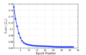
Figure 11: Convergence behavior of the proposed aperiodic SISO two-layer BiSCorN for the case of $N=400$.

V-A1 Convergence

The convergence of the proposed aperiodic SISO two-layer BiSCorN is shown in Fig. 11 via considering the values of the loss function in (12) for sequence length $N=400$ versus the number of epochs. It is observed that the loss function values have a monotonic descent property, as expected.

V-A2 Binarization Versus Sidelobe Minimization

TABLE II: The ISL Values and the Number of Non-Binary Elements in the Output Aperiodic Sequence of the SISO Single-Layer BiSCorN with Deterministic and Stochastic Inputs for Gradually Increasing the Weight Ratio WR and Different Values of $N$.

According to Lemma 1, the design problem in (4) can be dealt with via a stop-start procedure applied to problem in (5) with fixed $\bar{w}_{\mathcal{S},s}$ and increasing $\bar{w}_{\mathcal{S},b}$. To illustrate this, we consider both deterministic and random cases for single-layer BiSCorN. We define the weight ratio (WR) as ${\textrm{WR}}^{(i)}=\frac{\bar{w}^{(i)}_{\mathcal{S},b}}{\bar{w}_{\mathcal{S},s}}$. The results for deterministic case ${\textrm{WR}}^{(i)}=2^{(i-1)}$, $i\geq 1$, and different values of $N$ are reported in Table II. That is, the table includes the ISL values of the synthesized binary sequences (see Remark 1) as well as the number of non-binary elements. As expected, in terms of average performance, increasing WR leads to less non-binary elements; however, for WR greater than 4, the resulting ISL values are kept fixed. Considering the best performance over 10 trials, we observed no change in ISL values for WR grater than 2. As an example, the resulting sequence before synthesis stage is shown in Fig. 12 for $N=50$ and different values of WR. It can be seen that by increasing WR, the number of non-binary elements decreases; also, the absolute value of non-binary elements approaches $\{-1,+1\}$ as can be seen by considering $\textrm{WR}=8,16,32$. As to random case, from Lemma 1 and Subsection III-A one can write

Figure 12: The output aperiodic sequence of SISO single-layer BiSCorN with deterministic input without quantization for gradually increasing the weight ratio WR and $N=50$.

$$\;\widetilde{\mathbf{w}}=\begin{cases}\bar{{{w}}}_{\mathcal{S},b}={{\mu}}^{2}_{\mathcal{S},k}+p_{\mathcal{S},k},~{}~{}~{}~{}~{}~{}~{}~{}~{}k=1,\\ w_{k-1}\bar{{w}}_{\mathcal{S},s}={{\mu}}^{2}_{\mathcal{S},k}+p_{\mathcal{S},k},~{}~{}2\leq k\leq N.\end{cases}$$ (67)

Now, given $\widetilde{\mathbf{w}}$, (67) is a system of linear equations with multiple choices for $\bm{{\mu}}_{\mathcal{S}}$ and $\mathbf{{p}}_{\mathcal{S}}$. We set ${{\mu}}_{\mathcal{S},k}$ equal to $0.5$, ${{p}}_{\mathcal{S},k}$ equal to $\frac{{{\mu}}_{\mathcal{S},k}}{5}$, for $2\leq k\leq N$, and then gradually increase ${{\mu}}_{\mathcal{S},1}$ with ${{p}}_{\mathcal{S},1}=\frac{{{\mu}}_{\mathcal{S},1}}{5}$ to obtain WRs in Table II. Note that network inputs for various steps are statistically independent. The results for the random case are also given in Table II. Similar considerations as those for the deterministic case hold true. We herein remark the fact that employing BiSCorN in a stop-start procedure is associated with higher computational burden while the improvement in ISL values is not significant. Therefore, in the sequel, we present results employing BiSCorN without stop-start procedure. More precisely, for SISO and CSS we set $\textrm{WR}=1$, i.e., $w_{\mathcal{S},b}=w_{\mathcal{S},s}$ and $w_{\mathcal{C},b}=w_{\mathcal{C},s}$; then, for MIMO and MIMO-CSS cases we set $\textrm{WR}=N_{T}$, i.e., $w_{\mathcal{M},b}=N_{T}\hskip 1.0ptw_{\mathcal{M},s}$ and $w_{\mathcal{MC},b}=N_{T}\hskip 1.0ptw_{\mathcal{MC},s}$ based on our numerical observation (see Subsection V-B3).

V-A3 SISO ISL Minimization

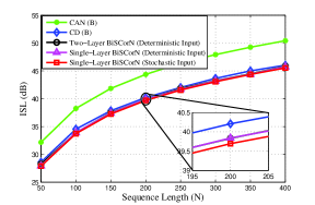
Figure 13: ISL of binary sequences obtained by BiSCorN, CAN (B), and CD (B) versus sequence length $N$ for the aperiodic ISL minimization problem.

Figure 14: The output sequence of the two-layer BiSCorN (without quantization) for $N=5$. The various rows in the figure are associated with different random initializations.

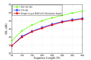
Figure 15: ISL of binary sequences obtained by BiSCorN, PeCAN (B), and CD (B) versus sequence length $N$ for the periodic ISL minimization problem.

The ISL versus the sequence length $N$ is shown in Fig. 13 for the aperiodic ISL minimization problem. We observe that the proposed BiSCorN has better performance than the benchmark methods, i.e., CAN (B) and CD (B), for the considered values of sequence length $N$. Specifically, the maximum ISL improvements of the single-layer BiSCorN for the case of stochastic input w.r.t. the CAN (B) and CD (B) are 4.90 dB and 0.82 dB, respectively.

Fig. 13 also shows the performance gain granted by the stochastic version of the input signal $\mathbf{s}_{\mathcal{S}}$ compared to the deterministic one; this can be explained using the fact that the ISL minimization is a multimodal problem and therefore the stochastic version of $\mathbf{s}_{\mathcal{S}}$ can help BiSCorN to achieve a better performance.

It is also numerically observed that the BiSCorN can produce Barker codes for the sequence lengths $N=2,3,4,5,7,11,13$ which confirm the effectiveness of the method. For instance, in Fig. 14, we employ the two-layer BiSCorN with $N=5$ and consider $10$ random initializations. It can be seen that in most of the instances, the resulting binary sequences are coincide with Barker codes.

Next, the ISL of the single-layer BiSCorN with stochastic input as well as that of benchmark methods is illustrated versus the sequence length $N$ for periodic ISL minimization in Fig. 15. In this case, the maximum performance gains of the proposed network w.r.t. PeCAN (B) and also CD (B) algorithms are 4.99 dB and 0.55 dB, respectively.

V-A4 SISO ISL Minimization with LCZ

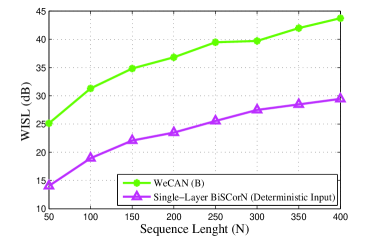
(a) $\widetilde{a}_{\mathcal{S},k}=1,~{}0\leq k\leq\lceil 0.1\times N\rceil,~{}~{}\widetilde{a}_{\mathcal{S},k}=0,~{}\textrm{otherwise}$.

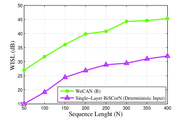
(b) $\widetilde{a}_{\mathcal{S},k}=1,~{}0\leq k\leq\lceil 0.2\times N\rceil,~{}~{}\widetilde{a}_{\mathcal{S},k}=0,~{}\textrm{otherwise}$.

Figure 16: WISL of binary sequences obtained by BiSCorN and WeCAN (B) versus sequence length $N$ for the aperiodic WISL minimization problem: (a) $\textrm{ROS}=10\%$, (b) $\textrm{ROS}=20\%$.

The performance of the proposed SISO BiSCorN is analyzed to design LCZ binary sequences. Let Region of Suppress (ROS) represents the set of lags associated with LCZ. Thus, the input signal $\mathbf{s}_{\mathcal{S}}$ must be compliant with the ROS and at the same time to balance between binarization and sidelobe minimization. Fig. 16 shows WISL of the single-layer BiSCorN with deterministic input compared to the WeCAN (B) for WISL minimization problem. Precisely, in Fig. 16.a and Fig. 16.b, respectively, the aim is to suppress the sidelobes $\left\{r(k)|_{k=1}^{\lceil 0.1\times N\rceil}\right\}$ and $\left\{r(k)|_{k=1}^{\lceil 0.2\times N\rceil}\right\}$ (corresponding to the ROS with $10\%$ and $20\%$ of all sidelobes). It can be seen from Fig. 16 that BiSCorN achieves significant smaller WISL than the benchmark method, i.e., WeCAN (B). Also, as an example the aperiodic auto-correlation function of the code obtained by single-layer BiSCorN along with the employed random initial sequence are illustrated in Fig. 17 for sequence length $N=1000$ and the ROS with $20\%$ of all sidelobes. This figure clearly unveils the effectiveness of the proposed BiSCorN.

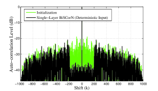
Figure 17: Auto-correlation level of binary sequence obtained by BiSCorN for the aperiodic WISL minimization problem with $N=1000$.

V-A5 PSL Evaluation

The PSL is now considered as a comparison metric that can be defined as

$$\textrm{PSL}=\max_{k}~{}|r(k)|,~{}~{}1\leq k\leq N-1.$$

The PSL values of the proposed ISL minimization algorithm BiSCorN, CAN (B), and CD (B) with pure PSL objective function, namely CD (B/PSL), are reported in Fig. 18 for the aperiodic case. Interestingly, it can be observed form Fig. 18 that the single-layer BiSCorN with stochastic input has smaller PSL than the benchmark methods for all values of the sequence length. The maximum PSL gains of the BiSCorN w.r.t. the CAN (B) and CD (B/PSL) are 3.03 dB and 0.56 dB, respectively. Fig. 18 also includes the PSL values for Minimum Peak Sidelobe (MPS) sequences [39] (known up to length 105) as well as the best PSL values associated with BiSCorN considering 10 independent trials.

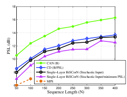
Figure 18: PSL of aperiodic binary sequences obtained by BiSCorN, CAN (B), and CD (B/PSL) versus the sequence length $N$.

V-B MIMO

The quantized Multi-CAN [13] and its weighted version, i.e., Multi-CAN (B) and WeMulti-CAN (B), as well as BiST method [21] are considered as benchmarks in this subsection. Note that the lower bound for ISL in the MIMO case is $N^{2}N_{T}(N_{T}-1)$ [14].

V-B1 MIMO ISL Minimization

In Fig. 19, the aperiodic ISL versus the sequence length $N$ is depicted for different number of transmit antennas $N_{T}\in\{3,4\}$. The figure shows that the BiSCorN (single-layer with deterministic input) exhibits better performance than BiST and Multi-CAN (B) for both the values of $N_{T}$ and also for the values of the sequence length $N$. The maximum ISL gains of the BiSCorN w.r.t. Multi-CAN (B) and BiST are 1.01 dB and 0.06 dB for $N_{T}=3$ and 0.75 dB and 0.03 dB for $N_{T}=4$. Interestingly, the ISL values of BiSCorN sequence sets are neighboring to around 0.2 dB and 0.1 dB of the lower bound for $N_{T}=3$ and $N_{T}=4$ respectively.

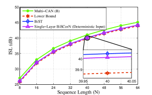
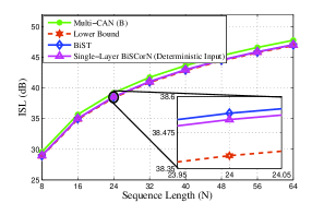
Figure 19: ISL of binary sequences obtained by BiSCorN, Multi-CAN (B), and BiST versus the sequence length $N$ for the aperiodic ISL minimization problem: (a) $N_{T}=3$, (b) $N_{T}=4$.

V-B2 MIMO ISL Minimization with LCZ

The performance of the MIMO BiSCorN to design LCZ sequences is now investigated. Fig. 20 illustrates the aperiodic WISL of the BiSCorN (single-layer with deterministic input) in comparison with WeMulti-CAN (B) for WISL minimization problem. In this case, the number of transmit antennas is set to $N_{T}=3$ and the ROS is equal to $20\%$ of all sidelobes i.e., $\left\{r(k)|_{k=1}^{\lceil 0.2\times N\rceil}\right\}$. The superior performance of the BiSCorN compared to WeMulti-CAN (B) can be observed from Fig. 20.

Figure 20: WISL of binary sequences obtained by BiSCorN and WeMulti-CAN (B) versus the sequence length $N$ for the aperiodic WISL minimization problem with $\textrm{ROS}=20\%$ and $N_{T}=3$.

V-B3 MIMO Binarization and Sidelobe Minimization Weights

As mentioned, we consider BiSCorN without stop-start procedure, viz. a fixed $\textrm{WR}=\frac{w_{\mathcal{M},b}}{w_{\mathcal{M},s}}$; then, herein, we study the effect of WR on the performance. For this purpose, the ISL values obtained by single-layer BiSCorN for the case of aperiodic MIMO versus $w_{\mathcal{M},b}$ are plotted in Fig. 21. This figure includes the behavior for different values of $N$ and $N_{T}$. It can be observed that for the current setup, a value of $w_{\mathcal{M},b}$ in the range of $[0.6,0.8]$ is a good choice. Considering $\textrm{WR}=\frac{w_{\mathcal{M},b}}{w_{\mathcal{M},s}}$ and $w_{\mathcal{M},b}+w_{\mathcal{M},s}=1$, the aforementioned interval of $w_{\mathcal{M},b}$ translates to $\textrm{WR}=N_{T}$.

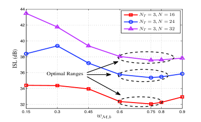
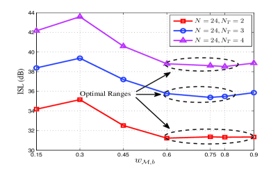
Figure 21: ISL of binary sequences obtained by BiSCorN versus binarization coefficient $w_{\mathcal{M},b}$ for the aperiodic ISL minimization problem: (a) $N_{T}=3$ and $N\in\{8,16,32\}$, (b) $N=24$ and $N_{T}\in\{2,3,4\}$.

V-C CSS

The binary version of the CANARY method [23], i.e., CANARY (B) is adopted as a benchmark in this subsection.

V-C1 CISL Minimization

In Fig. 22, the performance of the two-layer BiSCorN and CANARY (B) is considered for producing aperiodic binary complementary sequences where the normalized CISL (dB), i.e.,

$$\textrm{Normalized CISL (dB)}=20\hskip 2.0pt\textrm{log}_{10}\frac{\textrm{CISL}}{M},~{}~{}1\leq k\leq N-1,$$ (68)

is used as comparison metric. In this case, the number of complementary sequences is set to $M=3$. The results show that the BiSCorN outperforms CANARY (B) providing maximum gain of 0.94 dB.

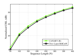
Figure 22: Normalized CISL of aperiodic binary complementary sequences obtained by BiSCorN and CANARY (B) versus sequence length $N$ for the case of $M=3$.

V-C2 CISL Minimization with LCZ

In Fig. 23 the aperiodic auto-correlation function of BiSCorN (single-layer with deterministic input) using different numbers of complementary sequences $M=1,2,3$ is illustrated for a sequence length $N=1000$ and a ROS=$20\%$. In this case, the auto-correlation sums are normalized and expressed in dB, i.e.,

$$\textrm{Auto-correlation Level (dB)}=20\hskip 2.0pt\textrm{log}_{10}\frac{w_{\mathcal{C},k}\left|\sum_{m^{\prime}=1}^{M}r_{m^{\prime}}(k)\right|}{\sum_{m^{\prime}=1}^{M}r_{m^{\prime}}(0)},~{}~{}1\leq k\leq N-1.$$ (69)

As expected, it can be observed that the auto-correlation level decreases as $M$ increases.

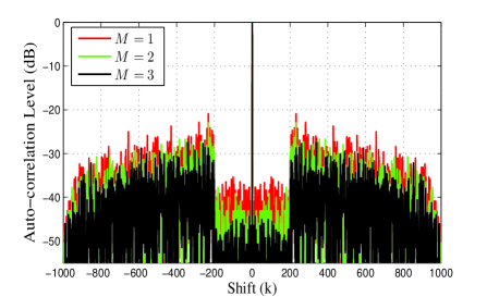
Figure 23: Auto-correlation level of aperiodic binary complementary sequences obtained by two-layer BiSCorN for a different number of complementary sequences $M=1,2,3$ with $N=1000$ and ROS=$20\%$.

V-D MIMO-CSS

The performance of MIMO-CSS systems (see Subsection III-D) is evaluated in this subsection. Fig. 24 shows normalized aperiodic CISL values of the MIMO two-layer BiSCorN versus the sequence length $N$ for different numbers of complementary sequences $M=1,2,3$. It is observed from this experiment that the MIMO complementary BiSCorN, i.e., the cases with $M=2,3$, achieves better performance than MIMO BiSCorN with $M=1$. Specifically, the maximum CISL gains of MIMO complementary BiSCorN for $M=3$ and $M=2$ w.r.t. the MIMO BiSCorN with $M=1$ are 9.75 dB and 4.91 dB, respectively.

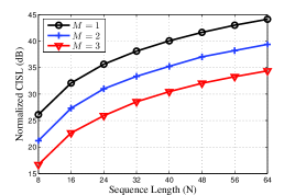
Figure 24: Normalized CISL of aperiodic binary complementary sequences obtained by MIMO two-layer BiSCorN versus the sequence length $N$ for different number of complementary sequences $M=1,2,3$.

VI Conclusion

The design of binary sequences with good aperiodic/periodic correlation properties has been considered, adopting the ISL as performance metric. In this respect, leveraging the asymptotic equivalence between the original design and its relaxed version, a novel learning-based framework denoted as BiSCorN, has been proposed for synthesizing binary (possibly complementary) sequences in SISO and MIMO systems. Then, network architectures have been devised to deal with a modified version of the ISL metric, i.e., weighted ISL. ADAM optimizer has been employed for the implementation of the BiSCorN learning process. Finally, a synthesis stage has been exploited to obtain feasible/binary solutions to the original problem, i.e., binary codes.

Numerical results have been provided to illustrate the effectiveness of the proposed learning-based approaches. In particular, it has been observed that the conceived architectures may outperform state-of-the-art algorithms for both SISO and MIMO systems in terms of ISL with a reasonable computational complexity. Future works may deal with designing binary sequences with good ambiguity function features, so as to deal with the presence of possible Doppler shifts.

Appendix A Proof of Lemma 1

Let us proceed by contradiction to prove the first item of the lemma. To this end, let us assume that the absolute value of at least one entry of $\mathbf{x}^{(i)}$ does not converge to one. This is tantamount to supposing that there exists a subsequence $\mathbf{x}^{(k_{i})}$ of $\mathbf{x}^{(i)}$ such that

$$\lim_{i\,\to\,+\infty} \displaystyle\min_{n=1,...,N} \left|x^{(k_{i})}(n)\right|<1,$$ (70)

which implies the existence of $0<\delta<1$ such that

$$\min_{n=1,...,N} \left|x^{(k_{i})}(n)\right|<(1-\delta),\,\,\mbox{provided that}\,\,i\,\,\mbox{is large enough}.$$ (71)

Before proceeding further, let us observe that any optimal solution to the original Problem (4) is a feasible point to Problem $\mathcal{P}^{(k_{i})}$, achieving ${w}_{\mathcal{S},s}^{(k_{i})}v^{\star}$ as objective value, with $v^{\star}$ the optimal value of (4). Moreover, based on (71), it follows

$$r^{(k_{i})}(0)=\sum_{n=1}^{N}|x^{(k_{i})}(n)|^{2}\leq N-1+(1-\delta)^{2}~{}\,\Leftrightarrow\,~{}N-r^{(k_{i})}(0)\geq 1-(1-\delta)^{2}.$$ (72)

As a consequence, denoting by $v\left(\mathcal{P}^{(k_{i})}\right)$ the optimal value to Problem $\mathcal{P}^{(k_{i})}$, the following inequality holds

$${w}_{\mathcal{S},s}^{(k_{i})}v^{\star}\geq v\left(\mathcal{P}^{(k_{i})}\right)\geq w_{\mathcal{S},b}^{(k_{i})}\left|1-(1-\delta)^{2}\right|^{2},$$ (73)

being $w_{\mathcal{S},s}^{(k_{i})}\sum_{k=1}^{N-1}w_{\mathcal{S},k}|r(k)|^{2}\geq 0$. Hence,

$$v^{\star}\geq\frac{\bar{w}^{(k_{i})}_{\mathcal{S},b}}{\bar{w}_{\mathcal{S},s}}\left|1-(1-\delta)^{2}\right|^{2},$$ (74)

which is evidently contradiction as $i\,\to\,+\infty$, since the right-hand side of the inequality goes to infinity while the left-hand side is a finite value. Therefore, $\left|x^{(i)}(n)\right|\,\to\,1$ for any $n$.

Let us now focus on the second item of the lemma. In this respect, let $\mathbf{x}^{(k_{i})}$ be a convergent subsequence of $\mathbf{x}^{(i)}$ with a limit point $\bar{\mathbf{x}}$ (its existence is guaranteed by the boundness of $\mathbf{x}^{(i)}$). Hence, denoting by $\mathbf{r}^{(k_{i})}$ and $\bar{\mathbf{r}}$ the auto-correlation vectors associated with $\mathbf{x}^{(k_{i})}$ and $\bar{\mathbf{x}}$, respectively, it follows that

$$\sum_{m=1}^{N-1}w_{\mathcal{S},m}\left|\bar{{r}}(m)\right|^{2}\geq v^{\star}.$$ (75)

Indeed, according to the first item of this lemma, at the limit point each entry of the sequence is unit modular and, therefore, the limit solution is a feasible point for the original problem in (4). Now, one can write

$$w_{\mathcal{S},s}^{(k_{i})}\sum_{m=1}^{N-1}w_{\mathcal{S},m}\left|{r}^{(k_{i})}(m)\right|^{2}\leq w_{\mathcal{S},b}^{(k_{i})}\left|{r}^{(k_{i})}(0)-N\right|^{2}+w_{\mathcal{S},s}^{(k_{i})}\sum_{m=1}^{N-1}w_{\mathcal{S},m}\left|{r}^{(k_{i})}(m)\right|^{2},~{}\forall i,$$ (76)

since $w_{\mathcal{S},b}^{(k_{i})}\left|{r}^{(k_{i})}(0)-N\right|^{2}\geq 0$. Then, note that any optimal solution to Problem (4) is a suboptimal solution to $\mathcal{P}^{(k_{i})}$, hence,

$$w_{\mathcal{S},b}^{(k_{i})}\left|{r}^{(k_{i})}(0)-N\right|^{2}+w_{\mathcal{S},s}^{(k_{i})}\sum_{m=1}^{N-1}w_{\mathcal{S},m}\left|{r}^{(k_{i})}(m)\right|^{2}\leq w_{\mathcal{S},s}^{(k_{i})}v^{\star},~{}\forall i.$$ (77)

Finally, (76) along with (77) implies that

$$\sum_{m=1}^{N-1}w_{\mathcal{S},m}\left|\bar{{r}}(m)\right|^{2}\leq v^{\star}.$$ (78)

By considering (75) and (78), it follows that $\bar{\mathbf{x}}$ is a binary sequence achieving the optimal auto-correlation sidelobes in terms of the WISL metric.

Appendix B The Derivation of (11) and (31)

First, considering (30), the matrix $\mathbf{X}_{\mathcal{C}}^{T}\mathbf{X}_{\mathcal{C}}$ can be expressed as the following

$${\begin{bmatrix}\sum_{m^{\prime}=1}^{M}r_{m^{\prime}}(0),&\sum_{m^{\prime}=1}^{M}r_{m^{\prime}}(1),&\sum_{m^{\prime}=1}^{M}r_{m^{\prime}}(2),&...,&\sum_{m^{\prime}=1}^{M}r_{m^{\prime}}(N-1)\\ \sum_{m^{\prime}=1}^{M}r_{m^{\prime}}(1),&\sum_{m^{\prime}=1}^{M}r_{m^{\prime}}(0),&\sum_{m^{\prime}=1}^{M}r_{m^{\prime}}(1),&...,&\sum_{m^{\prime}=1}^{M}r_{m^{\prime}}(N-2)\\ \vdots&\vdots&\vdots&&\vdots\\ \sum_{m^{\prime}=1}^{M}r_{m^{\prime}}(N-1),&\sum_{m^{\prime}=1}^{M}r_{m^{\prime}}(N-2),&\sum_{m^{\prime}=1}^{M}r_{m^{\prime}}(N-3),&...,&\sum_{m^{\prime}=1}^{M}r_{m^{\prime}}(0)\end{bmatrix}}\in\mathbb{R}^{N\times N}.$$ (79)

Note that $\mathbf{X}_{\mathcal{S}}^{T}\mathbf{X}_{\mathcal{S}}$ can be obtained from the matrix in (79) setting $M=1$. Then, using (79), the output signal for SISO system is given by

$$\mathbf{y}_{\mathcal{S}}=\mathbf{X}^{T}_{\mathcal{S}}\mathbf{X}_{\mathcal{S}}\mathbf{s}_{\mathcal{S}}={\begin{bmatrix}s_{\mathcal{S},1}r(0)+s_{\mathcal{S},2}r(1)+...+s_{\mathcal{S},N}r(N-1)\\ s_{\mathcal{S},1}r(1)+s_{\mathcal{S},2}r(0)+...s_{\mathcal{S},N}r(N-2)\\ \vdots\\ s_{\mathcal{S},1}r(N-1)+s_{\mathcal{S},2}r(N-2)+...+s_{\mathcal{S},N}r(0)\end{bmatrix}}\in\mathbb{R}^{N}.$$

Now, it is verified that the $k^{th}$ entry of $\mathbf{y}_{\mathcal{S}}$ can be expressed as in (11).

Next, considering the input signal $\mathbf{s}_{\mathcal{C}}=[{a}_{\mathcal{C}},0,0,...,0]\in\mathbb{R}^{N}$ from Subsection II-C and using the matrix in (79), the output vector for the CSS case can be obtained as

$$\mathbf{y}_{\mathcal{C}}=\mathbf{X}_{\mathcal{C}}^{T}\mathbf{X}_{\mathcal{C}}\hskip 1.0pt\mathbf{s}_{\mathcal{C}}={a_{\mathcal{C}}}\hskip 2.0pt{\begin{bmatrix}\sum_{m^{\prime}=1}^{M}r_{m^{\prime}}(0)\\ \sum_{m^{\prime}=1}^{M}r_{m^{\prime}}(1)\\ \vdots\\ \sum_{m^{\prime}=1}^{M}r_{m^{\prime}}(N-1)\end{bmatrix}}\in\mathbb{R}^{N}.$$ (80)

Finally, using (80) and (29), the loss function in (31) can be achieved.

Appendix C The Derivation of (24) and (38)

Considering (36) we can write

$$\mathbf{X}_{\mathcal{MC}}^{T}\mathbf{X}_{\mathcal{MC}}={\begin{bmatrix}\mathbf{R}_{11},&\mathbf{R}_{12},&...,&\mathbf{R}_{1N_{T}}\\ \mathbf{R}_{21},&\mathbf{R}_{22},&...,&\mathbf{R}_{2N_{T}}\\ \vdots&\vdots&&\vdots\\ \mathbf{R}_{N_{T}1},&\mathbf{R}_{N_{T}2},&...,&\mathbf{R}_{N_{T}N_{T}}\end{bmatrix}}\in\mathbb{R}^{NN_{T}\times NN_{T}},$$ (81)

where $\mathbf{R}_{ij}=\sum_{m^{\prime}=1}^{M}\mathbf{R}_{ij,m^{\prime}},~{}i,j=1,...,N_{T},$ and

$$\mathbf{R}_{ij,m^{\prime}}={\begin{bmatrix}r_{ij,m^{\prime}}(0),&\sqrt{2}\hskip 2.0ptr_{ij,m^{\prime}}(1),&\sqrt{2}\hskip 2.0ptr_{ij,m^{\prime}}(2),&...,&\sqrt{2}\hskip 2.0ptr_{ij,m^{\prime}}(N-1)\\ \sqrt{2}\hskip 2.0ptr_{ij,m^{\prime}}(1),&2\hskip 2.0ptr_{ij,m^{\prime}}(0),&2\hskip 2.0ptr_{ij,m^{\prime}}(1),&...,&2\hskip 2.0ptr_{ij,m^{\prime}}(N-2)\\ \vdots&\vdots&\vdots&&\vdots\\ \sqrt{2}\hskip 2.0ptr_{ij,m^{\prime}}(N-1),&2\hskip 2.0ptr_{ij,m^{\prime}}(N-2),&2\hskip 2.0ptr_{ij,m^{\prime}}(N-3),&...,&2\hskip 2.0ptr_{ij,m^{\prime}}(0)\end{bmatrix}}\in\mathbb{R}^{N\times N}.$$ (82)

Next, according to the input matrix $\mathbf{S}_{\mathcal{MC}}$ in (37), the output matrix becomes

$$\mathbf{Y}_{\mathcal{MC}}=\mathbf{X}_{\mathcal{MC}}^{T}\mathbf{X}_{\mathcal{MC}}\mathbf{S}_{\mathcal{MC}}={\begin{bmatrix}\widetilde{\mathbf{R}}_{1}\\ \widetilde{\mathbf{R}}_{2}\\ \vdots\\ \widetilde{\mathbf{R}}_{N_{T}}\end{bmatrix}}\in\mathbb{R}^{NN_{T}\times N_{T}},$$ (83)

where $\widetilde{\mathbf{R}}_{i}=\sum_{m^{\prime}=1}^{M}\widetilde{\mathbf{R}}_{i,m^{\prime}},~{}i=1,...,N_{T},$ and

$$\widetilde{\mathbf{R}}_{i,m^{\prime}}={a_{\mathcal{M}}}\hskip 2.0pt{\begin{bmatrix}r_{i1,m^{\prime}}(0),&r_{i2,m^{\prime}}(0),&...,&r_{iN_{T},m^{\prime}}(0)\\ \sqrt{2}\hskip 2.0ptr_{i1,m^{\prime}}(1),&\sqrt{2}\hskip 2.0ptr_{i2,m^{\prime}}(1),&...,&\sqrt{2}\hskip 2.0ptr_{iN_{T},m^{\prime}}(1)\\ \vdots&\vdots&&\vdots\\ \sqrt{2}\hskip 2.0ptr_{i1,m^{\prime}}(N-1),&\sqrt{2}\hskip 2.0ptr_{i2,m^{\prime}}(N-1),&...,&\sqrt{2}\hskip 2.0ptr_{iN_{T},m^{\prime}}(N-1)\end{bmatrix}}\in\mathbb{R}^{N\times N_{T}}.$$ (84)

Therefore, using the output matrix in (83) and considering (35), the loss function in (38) is given by $\mathcal{L}_{\mathcal{MC}}=\mathbf{a}^{T}_{\mathcal{MC}}\hskip 1.0pt\widetilde{\mathbf{r}}_{\mathcal{MC}}$. Also, the loss function of the MIMO radar in (24) can be obtained using a similar procedure as in (81)-(84) considering $M=1$.

References

- [1] H. He, J. Li, and P. Stoica, Waveform design for active sensing systems: a computational approach. Cambridge University Press, 2012.
- [2] F. Gini, A. De Maio, and L. Patton, Waveform design and diversity for advanced radar systems. Institution of engineering and technology London, UK, 2012.
- [3] A. Aubry, A. De Maio, and M. M. Naghsh, “Optimizing radar waveform and Doppler filter bank via generalized fractional programming,” IEEE Journal of Selected Topics in Signal Processing, vol. 9, no. 8, pp. 1387–1399, 2015.
- [4] M. Skolnik, Radar Handbook, Third Edition, ser. Electronics electrical engineering. McGraw-Hill Education, 2008. [Online]. Available: https://books.google.com/books?id=76uF2Xebm-gC
- [5] M. Friese, “Polyphase barker sequences up to length 36,” IEEE Transactions on Information Theory, vol. 42, no. 4, pp. 1248–1250, 1996.
- [6] P. Borwein and R. Ferguson, “Polyphase sequences with low autocorrelation,” IEEE Transactions on Information Theory, vol. 51, no. 4, pp. 1564–1567, 2005.
- [7] C. Nunn, “Constrained optimization applied to pulse compression codes and filters,” in IEEE International Radar Conference, 2005. IEEE, 2005, pp. 190–194.
- [8] C. J. Nunn and G. E. Coxson, “Polyphase pulse compression codes with optimal peak and integrated sidelobes,” IEEE Transactions on Aerospace and Electronic Systems, vol. 45, no. 2, pp. 775–781, 2009.
- [9] P. Stoica, H. He, and J. Li, “New algorithms for designing unimodular sequences with good correlation properties,” IEEE Transactions on Signal Processing, vol. 57, no. 4, pp. 1415–1425, 2009.
- [10] R. Lin, M. Soltanalian, B. Tang, and J. Li, “Efficient design of binary sequences with low autocorrelation sidelobes,” IEEE Transactions on Signal Processing, vol. 67, no. 24, pp. 6397–6410, 2019.
- [11] J. Song, P. Babu, and D. P. Palomar, “Sequence design to minimize the weighted integrated and peak sidelobe levels,” IEEE Transactions on Signal Processing, vol. 64, no. 8, pp. 2051–2064, 2015.
- [12] M. A. Kerahroodi, A. Aubry, A. De Maio, M. M. Naghsh, and M. Modarres-Hashemi, “A coordinate-descent framework to design low PSL/ISL sequences,” IEEE Transactions on Signal Processing, vol. 65, no. 22, pp. 5942–5956, 2017.
- [13] H. He, P. Stoica, and J. Li, “Designing unimodular sequence sets with good correlations; including an application to MIMO radar,” IEEE Transactions on Signal Processing, vol. 57, no. 11, pp. 4391–4405, 2009.
- [14] J. Song, P. Babu, and D. P. Palomar, “Sequence set design with good correlation properties via majorization-minimization,” IEEE Transactions on Signal Processing, vol. 64, no. 11, pp. 2866–2879, 2016.
- [15] Y. Li, S. A. Vorobyov, and Z. He, “Design of multiple unimodular waveforms with low auto-and cross-correlations for radar via majorization-minimization,” in 2016 24th European Signal Processing Conference (EUSIPCO). IEEE, 2016, pp. 2235–2239.
- [16] Y. Li and S. A. Vorobyov, “Fast algorithms for designing unimodular waveform (s) with good correlation properties,” IEEE Transactions on Signal Processing, vol. 66, no. 5, pp. 1197–1212, 2017.
- [17] G. Cui, X. Yu, M. Piezzo, and L. Kong, “Constant modulus sequence set design with good correlation properties,” Signal Processing, vol. 139, pp. 75–85, 2017.
- [18] J. Tang, N. Zhang, Z. Ma, and B. Tang, “Construction of Doppler resilient complete complementary code in MIMO radar,” IEEE Transactions on Signal Processing, vol. 62, no. 18, pp. 4704–4712, 2014.
- [19] J. Wang and Y. Wang, “Designing unimodular sequences with optimized auto/cross-correlation properties via consensus-ADMM/PDMM approaches,” IEEE Transactions on Signal Processing, vol. 69, pp. 2987–2999, 2021.
- [20] M. Soltanalian, M. M. Naghsh, and P. Stoica, “On meeting the peak correlation bounds,” IEEE Transactions on Signal Processing, vol. 62, no. 5, pp. 1210–1220, 2014.
- [21] M. Alaee-Kerahroodi, M. Modarres-Hashemi, and M. M. Naghsh, “Designing sets of binary sequences for MIMO radar systems,” IEEE Transactions on Signal Processing, vol. 67, no. 13, pp. 3347–3360, 2019.
- [22] M. Soltanalian and P. Stoica, “Computational design of sequences with good correlation properties,” IEEE Transactions on Signal processing, vol. 60, no. 5, pp. 2180–2193, 2012.
- [23] M. Soltanalian, M. M. Naghsh, and P. Stoica, “A fast algorithm for designing complementary sets of sequences,” Signal Processing, vol. 93, no. 7, pp. 2096–2102, 2013.
- [24] J. Wang, P. Fan, Z. Zhou, and Y. Yang, “Quasi-orthogonal z-complementary pairs and their applications in fully polarimetric radar systems,” IEEE Transactions on Information Theory, 2021.
- [25] Z.-J. Wu, T.-L. Xu, Z.-Q. Zhou, and C.-X. Wang, “Fast algorithms for designing complementary sets of sequences under multiple constraints,” IEEE Access, vol. 7, pp. 50 041–50 051, 2019.
- [26] J. Chai, H. Zeng, A. Li, and E. W. Ngai, “Deep learning in computer vision: A critical review of emerging techniques and application scenarios,” Machine Learning with Applications, vol. 6, p. 100134, 2021.
- [27] M. Ahmadi, A. Norouzi, N. Karimi, S. Samavi, and A. Emami, “Redmark: Framework for residual diffusion watermarking based on deep networks,” Expert Systems with Applications, p. 113157, 2019.
- [28] S. Khobahi and M. Soltanalian, “Model-based deep learning for one-bit compressive sensing,” IEEE Transactions on Signal Processing, vol. 68, pp. 5292–5307, 2020.
- [29] Y. Zeng, X. Xu, S. Jin, and R. Zhang, “Simultaneous navigation and radio mapping for cellular-connected uav with deep reinforcement learning,” IEEE Transactions on Wireless Communications, 2021.
- [30] M. K. Sharma, A. Zappone, M. Assaad, M. Debbah, and S. Vassilaras, “Distributed power control for large energy harvesting networks: A multi-agent deep reinforcement learning approach,” IEEE Transactions on Cognitive Communications and Networking, vol. 5, no. 4, pp. 1140–1154, 2019.
- [31] C. D’Andrea, A. Zappone, S. Buzzi, and M. Debbah, “Uplink power control in cell-free massive MIMO via deep learning,” in 2019 IEEE 8th International Workshop on Computational Advances in Multi-Sensor Adaptive Processing (CAMSAP). IEEE, 2019, pp. 554–558.
- [32] O. Rezaei, M. Ahmadi, and M. M. Naghsh, “A learning approach to design binary sequences with good correlation properties,” in 2020 IEEE Radar Conference (RadarConf20). IEEE, 2020, pp. 1–6.
- [33] G. E. Hinton and R. S. Zemel, “Autoencoders, minimum description length and Helmholtz free energy,” in Advances in neural information processing systems, 1994, pp. 3–10.
- [34] P. Li and P.-M. Nguyen, “On random deep weight-tied autoencoders: Exact asymptotic analysis, phase transitions, and implications to training,” in International Conference on Learning Representations, 2018.
- [35] M. Courbariaux, I. Hubara, D. Soudry, R. El-Yaniv, and Y. Bengio, “Binarized neural networks: Training deep neural networks with weights and activations constrained to+ 1 or-1,” arXiv preprint arXiv:1602.02830, 2016.
- [36] M. Abadi, P. Barham, J. Chen, Z. Chen, A. Davis, J. Dean, M. Devin, S. Ghemawat, G. Irving, M. Isard et al., “Tensorflow: A system for large-scale machine learning,” in 12th USENIX Symposium on Operating Systems Design and Implementation (OSDI 16), 2016, pp. 265–283.
- [37] D. P. Kingma and J. Ba, “Adam: A method for stochastic optimization,” in ICLR, 2015.
- [38] I. Goodfellow, Y. Bengio, and A. Courville, Deep learning. MIT press, 2016.
- [39] C. J. Nunn and G. E. Coxson, “Best-known autocorrelation peak sidelobe levels for binary codes of length 71 to 105,” IEEE transactions on Aerospace and Electronic Systems, vol. 44, no. 1, pp. 392–395, 2008.