Rejection-free quantum Monte Carlo in continuous time from transition path sampling

Abstract

Continuous-time quantum Monte Carlo refers to a class of algorithms designed to sample the thermal distribution of a quantum Hamiltonian through exact expansions of the Boltzmann exponential in terms of stochastic trajectories which are periodic in imaginary time. Here, we show that for (sign-problem-free) quantum many-body systems with discrete degrees of freedom — such as spins on a lattice — this sampling can be done in a rejection-free manner using transition path sampling (TPS). The key idea is to converge the trajectory ensemble through updates where one individual degree of freedom is modified across all time while the remaining unaltered ones provide a time-dependent background. The ensuing single-body dynamics provides a way to generate trajectory updates exactly, allowing one to obtain the target ensemble efficiently via rejection-free TPS. We demonstrate our method on the transverse field Ising model in one and two dimensions, and on the quantum triangular plaquette (or Newman-Moore) model. We show that despite large autocorrelation times, our method is able to efficiently recover the respective quantum phase transition of each model. We also discuss the connection to rare event sampling in continuous-time Markov dynamics.

I Introduction

Statistical mechanics has facilitated the study of many-body systems through Monte Carlo sampling for several decades. Originally developed for classical Hamiltonians, classical Monte Carlo methods allow the sampling of the Boltzmann distribution by proposing updates to a configuration together with a criterion, such as Metropolis [1, 2] or Glauber [3], to accept or reject the changes. At the same time, Monte Carlo sampling can be generalized to study the Boltzmann distribution of quantum many-body Hamiltonians [4]. However, a complication here is that the weights of the configurations require the evolution to be computed in imaginary time.

A standard approach is to split the imaginary-time evolution of the quantum partition sum into discrete timesteps, giving rise to “trajectories” of configurations in discretized imaginary-time, where the weightings of the trajectories can be estimated for small timesteps through a Trotter-Suzuki decomposition [5, 6]. This procedure can be made exact by considering a continuous-time expansion instead, in terms of a perturbative expansion of the Boltzmann exponential in the interaction picture and to all orders, yielding a sum over classical trajectories in continuous-time [7, 8, 9, 10]. In either of these approaches, there is added complexity in relation to the classical case, as imaginary-time trajectories have to be sampled by making changes to the temporal degrees of freedom in addition to the spatial ones .

In this paper we focus on the continuous-time expansion of the quantum Boltzmann distribution through trajectory ensembles. For systems with discrete local degrees of freedom (and in the absence of a sign problem [12, 13]) we show how the trajectories that define the quantum partition sum can be sampled through the realization of the so-called Doob dynamics (see e.g. Refs. [14, 15, 16]), which optimally samples rare events. Specifically, we show how this can be achieved efficiently through exact trajectory updates which are local in space but extensive in time. In this way we can generate ensembles of trajectories using a version of transition path sampling (TPS) which is rejection-free.

We illustrate the method by studying the transverse field Ising model (TFIM) in one and two spatial dimensions. In this case we sample many-body trajectories by updating the trajectories of individual spins, while keeping the other spins as an effective time-dependent background. This approach is equivalent to the one in Ref. [17], which studied the TFIM on the Bethe lattice, and to the one in Ref. [18], which studied transition events of the classical 2D Ising model. Here, we demonstrate that this approach is capable of predicting the well known continuous phase transitions for the 1D and 2D TFIM, despite the fact that the local updates suffer from large autocorrelation times close to criticality.

We also show how to use our approach with more complex spin interactions by means of customized local updates. As a concrete example, we study the quantum Newman-Moore model [19, 20, 21, 22, 23, 24, 25], also known as the quantum triangular plaquette model (QTPM). This model builds on the classical TPM [26, 27, 28], a system of spins with three-body interactions studied in the context of glasses, making it quantum by adding a transverse magnetic field. For the QTPM we devise local updates by simultaneously changing the trajectories of three neighbouring spins. Our method can effectively recover the first-order quantum phase transition of the QTPM [19, 20, 22, 23, 24]. We further show how thermal annealing can be implemented to improve sampling close to the transition point.

The paper is structured as follows. Section II formalizes the connection between the quantum Boltzmann distribution and rare-trajectory sampling, explaining how observables can be estimated from trajectories. Section III then explains how the optimal Doob dynamics can be used to sample trajectories from the quantum Boltzmann distribution. Section IV demonstrates how this approach can be used to incorporate a single-spin update scheme for spin models with a simple transverse field, in analogy to Ref. [17], by implementing the method for the 1D and 2D TFIM. Section V generalizes the method to Hamiltonians with more complex interaction terms, using the QTPM as a concrete example. We give our conclusions in Sec. VI, where we discuss the possibility of more involved schemes, including updates which are collective in space. This approach is presented in Appendix B, where it is also extended to sample rare events in classical continuous-time Markov dynamics, determining the dynamical large deviations (LDs) of the TFIM and QTPM as an example.

II Monte Carlo sampling of the Boltzmann distribution

II.1 The quantum partition function and continuous-time stochastic dynamics

We consider a system with a Hamiltonian $\hat{H}$ and a discrete set of configurations that defines a basis $\{\ket{x}\}$ of its Hilbert space, $\mathscr{H}$. In this basis, the Hamiltonian can be decomposed into a diagonal part and an off-diagonal part, $\hat{H}=\hat{H}^{\rm c}-\hat{K}$,

$$\hat{H}^{\rm c}=\sum_{x}H^{c}_{x}\ket{x}\bra{x},$$ (1)

$$\hat{K}=\sum_{x,y\neq x}\hat{K}_{x\to y}\equiv\sum_{x,y\neq x}K_{x\to y}\ket{y}\bra{x}.$$ (2)

We will refer to operators which act on the whole Hilbert space by symbols with a hat (e.g. $\hat{H}^{c}$), and their individual matrix elements by symbols without a hat.

The statistical properties of $\hat{H}$ at some finite temperature are characterized by the partition function,

$$Z_{\beta}=\operatorname{Tr}\left[e^{-\beta\hat{H}}\right]=\sum_{x}\braket{x}{e^{-\beta\hat{H}}}{x}.$$ (3)

Equation (3) can be expressed as a sum over stochastic paths by considering its Dyson series expansion [29],

$$Z_{\beta}=\sum_{M=0}^{\infty}\sum_{x_{\mkern-0.5mu0},\cdots,x_{\mkern-2.0muM}}\int dt_{\mkern-2.0muM}\dots dt_{1}\bra{x_{0}}e^{-(\beta-t_{\mkern-2.0muM})\hat{H}^{\rm c}}\\ \prod_{m=1}^{M}\left[\hat{K}_{x_{\mkern-1.0mum-1}\to x_{\mkern-1.0mum}}e^{-(t_{m}-t_{m-1})\hat{H}^{\rm c}}\right]\ket{x_{0}},$$ (4)

where the integrals over times $t_{m}$ are performed with the limits $\beta\geq t_{\mkern-2.0muM}\geq\dots\geq t_{0}$. Note that the product in Eq. (4) is omitted for the case of $M=0$.

Each path in Eq. (4) can be interpreted as a classical stochastic trajectory in continuous-time with time extent $\beta$, where the operator $\hat{K}_{x_{m-1}\to x_{m}}$ makes the instantaneous transition $x_{m-1}\to x_{m}$ at the time $t_{m}$. We denote a stochastic trajectory of time extent $\beta$ with $M$ jumps as

$${\bm{x}}=\{(t_{0},x_{0}),\dots,(t_{\mkern-1.0muM},x_{\mkern-1.4muM})\},$$ (5)

(note that the last jump occurs at $t_{M}\leq\beta$). We then represent Eq. (4) as a sum over these jumps,

$$Z_{\beta}=\sum_{\{{\bm{x}}\}}\delta_{x(0),x(\beta)}e^{-\int_{0}^{\beta}dt\,H^{\rm c}_{x(t)}}\prod_{m=1}^{\mathcal{K}\mkern-1.0mu({\mkern-0.4mu\bm{x}\mkern-0.4mu})}K_{x_{m-1}\to x_{m}},$$ (6)

where ${x}(t)$ denotes the configuration of the trajectory ${\bm{x}}$ at time $t$, $\delta_{x(0),x(\beta)}$ allows only for trajectories which are periodic in time, and $\mathcal{K}({\bm{x}})$ is the trajectory observable (which will henceforth be denoted by a calligraphic font) which returns the number of transitions which occur in the trajectory. The sum over $\{{\bm{x}}\}$ indicates a sum over all paths for any number of jumps, $M\in[0,\infty)$. We can then write the probability of the trajectory ${\bm{x}}$ as

$$P_{\beta}({\bm{x}})=\frac{1}{Z_{\beta}}\delta_{x(0),x(\beta)}e^{-\int_{0}^{\beta}dt\,H^{\rm c}_{{x}(t)}}\prod_{m=1}^{\mathcal{K}\mkern-1.0mu({\mkern-0.4mu\bm{x}\mkern-0.4mu})}K_{x_{m-1}\to x_{m}}.$$ (7)

The probability Eq. (7) can be related to that for trajectories generated by a continuous-time Markov dynamics in the following way. We define the Markov generator $\hat{W}=\hat{K}-\hat{R}$, with the transitions given by $\hat{K}$ and their associated escape rates, $\hat{R}$,

$$\hat{R}=\sum_{x,y\neq x}K_{x\to y}\ket{x}\bra{x}=\sum_{x}R_{x}\ket{x}\bra{x}.$$ (8)

Since we consider quantum systems without a sign problem [12, 13], we can assume that the probabilities Eq. (7) are positive real numbers. With these definitions, the relation between the Hamiltonian and the stochastic generator is

$$\hat{H}=-(\hat{W}+\hat{R}-\hat{H}^{\rm c}).$$ (9)

It follows that the trajectories that define the partition function Eq. (6) are related to those generated by the stochastic dynamics of $\hat{W}$ with the following properties:

1. The trajectory must start and finish in the same configuration, i.e., it should be a stochastic bridge. A trajectory which does not meet this criterion has zero probability of occurring.

2. The probability of a trajectory that satisfies (i) is exponentially biased (with respect to the probability of occurring under $\hat{W}$) by the time integral of $\hat{H}^{\rm c}-\hat{R}$ along the trajectory. That is, its probability is multiplied by the factor $e^{-\int_{0}^{\beta}d\tau\,\left(H^{\rm c}_{{x}(t)}-R_{{x}(t)}\right)}$.

Condition (i) is needed due to the imposition of periodic paths in Eq. (4). The bias in (ii) accounts for the difference in the diagonal parts of $\hat{W}$ and $\hat{H}$. Many methods have been developed to efficiently sample biased dynamics as in (ii). One popular approach is transition path sampling (TPS), see e.g. Refs. [30, 31, 22]. Here, we will use TPS focusing on techniques for sampling trajectory updates which are local in space, cf. Refs. [17, 18], and which also account for (i).

II.2 Calculating observables

The thermal expectation value of an observable $\hat{O}$ is given by,

$$\braket{\hat{O}}_{\beta}=\frac{\sum_{x}\braket{x}{\hat{O}\,e^{-\beta\hat{H}}}{x}}{Z_{\beta}}.$$ (10)

This can be rewritten as an imaginary-time average by noticing that we can arbitrarily move $\hat{O}$ through the exponential due to the properties of the trace,

$$\braket{\hat{O}}_{\beta}=\frac{1}{\beta}\int_{0}^{\beta}dt\,\frac{\sum_{x}\braket{x}{e^{-(\beta-t)\hat{H}}\hat{O}e^{-t\hat{H}}}{x}}{Z_{\beta}}.$$ (11)

In order to consider how to compute Eq. (11) from trajectories we will deal separately with the cases when $\hat{O}$ is diagonal and off-diagonal.

For the case of a diagonal operator, $\hat{O}_{\rm diag}=\sum_{x}O(x)\ket{x}\bra{x}$, Eq. (11) can be directly written as a sum over all trajectories with the probability given by Eq. (7). This leads to

$$\braket{\hat{O}_{\rm diag}}_{\beta}=\beta^{-1}\sum_{\{{\bm{x}}\}}P_{\beta}({\bm{x}})\mathcal{O}({\bm{x}}),$$ (12)

where $\mathcal{O}({\bm{x}})=\int_{0}^{\beta}dt\,O({x}(t))$ is the time-integrated trajectory observable. That is, we average the value of the observable over all times and over all trajectories.

For an off-diagonal operator, $\hat{O}_{\rm off-diag}=\sum_{y\neq x}O_{x\to y}\ket{y}\bra{x}$, we can expand both exponentials in Eq. (11). This expansion in the integrand of Eq. (11) gives a sum over all trajectories which have the transition $x\to y$ at the time $t$, summed over $y\neq x$. Compared to Eq. (6), the jumps at time $t$ appear with factors $O_{x\to y}$ rather than $K_{x\to y}$. Thus, if we want to express $\braket{\hat{O}_{\rm off-diag}}$ as a sum over trajectories with the probability given by Eq. (7), we need to account for the change $K_{x\to y}\to O_{x\to y}$ at time $t$. Furthermore, since we are time averaging, we can replace the integration over time by $N_{x\to y}({\bm{x}})$ which counts the number of jumps $x\to y$ which occur in trajectory ${\bm{x}}$. We can then write

$$\braket{\hat{O}_{\rm off-diag}}_{\beta}=\beta^{-1}\sum_{\{{\bm{x}}\}}P_{\beta}({\bm{x}})\sum_{x\neq y}\frac{N_{x\to y}({\bm{x}})}{K_{x\to y}}O_{x\to y}.$$ (13)

III Optimal sampling

We now explain how trajectories can be sampled efficiently and exactly from the partition function Eq. (6) by means of a rejection-free form of TPS. A general method for converging to an ensemble of trajectories such as Eq. (7) is TPS, a form of Monte Carlo sampling in trajectory space [30]. A typical problem with standard TPS is that acceptance of trajectory updates can become exponentially small in system size (and/or the length of the trajectory), thus slowing down convergence.

In the language of stochastic dynamics, the procedure we now describe is sometimes referred to as obtaining the Doob dynamics [14, 15, 16], a proper (normalized) stochastic dynamics derived from the original generator $\hat{W}$, which generates trajectories with a conditioned/biased probability $P_{\beta}({\bm{x}})$ such as Eq. (7). While this approach is exact in theory, it often relies on the computation of expressions which are, in practice, analytically (and often numerically) intractable. However, we will show later in the paper that we can in fact implement this general idea via optimal local updates.

III.1 Edge configurations

The first obstacle is to sample the initial/final configuration of trajectories, $x_{0}$. While Eq. (6) has no explicit probability distribution for the initial configuration $x_{0}$, its probability will be decided by its possible transitions and its diagonal component in Eq. (1). That is, we choose some initial configuration, $x_{0}$, with probability

$$P(x_{0})=\frac{\braket{x_{0}}{e^{-\beta\hat{H}}}{x_{0}}}{Z_{\beta}}.$$ (14)

Once the trajectory edges have been selected, we can then sample the remainder of the trajectory from the subset of trajectories which have the required boundary conditions. That is, we want to sample from the reduced dynamics

$$Z_{\beta}(x_{\rm i},x_{\rm f})=\braket{x_{\rm f}}{e^{-\beta\hat{H}}}{x_{\rm i}},$$ (15)

where $x_{\rm i}$ and $x_{\rm f}$ are the initial and final configurations. Note that, although we are only interested in trajectories which have $x_{\rm i}=x_{\rm f}$, it will be useful to solve this more general problem for later for the TFIM and QTPM.

III.2 Continuous-time dynamics

To sample the dynamics, we will employ the continuous-time Monte Carlo (CTMC) method, also known as the Bortz-Kalos-Lebowitz, the rejection-free kinetic Monte Carlo, or the Gillespie algorithm [32, 33, 34]. While this method is straightforward for a normalized time-homogeneous dynamics, it will be useful to formulate the general case of time-dependent dynamics for what follows.

Consider time-dependent instantaneous transition rates, $\tilde{K}_{x\to y}(t;\beta,x_{\rm f})\geq 0$, for transitions from configuration $x$ to configuration $y$ at time $t\leq\beta$. We use the tilde to distinguish these from the off-diagonal entries of the Hamiltonian, cf. Eq. (2), and also allow for a dependence on the final configuration, $x_{\rm f}$, and the overall trajectory time, $\beta$. The associated escape rate from configuration $x$ at time $t$ is

$$\tilde{R}_{x}(t;\beta,x_{\rm f})=\sum_{y\neq x}\tilde{K}_{x\to y}(t;\beta,x_{\rm f}).$$ (16)

The escape rate in turn determines the distribution of the waiting time $\tau$, $P_{x}$, for a jump out of $x$ after $t$,

$$P_{x}(\tau;t,\beta,x_{\rm f})=\tilde{R}_{x}(t+\tau;\beta,x_{\rm f})\\ \exp\left[-\int_{t}^{t+\tau}dt^{\prime}\,\tilde{R}_{x}(t^{\prime};\beta,x_{\rm f})\right].$$ (17)

After a waiting time has been drawn from Eq. (17), the transition into $y$ at time $t+\tau$ is chosen with probability

$$P_{x}(y\,|\,t+\tau;\,\beta,x_{\rm f})=\frac{\tilde{K}_{x\to y}(t+\tau;\beta,x_{\rm f})}{\sum_{z\neq x}\tilde{K}_{x\to z}(t+\tau;\beta,x_{\rm f})}.$$ (18)

III.3 Optimal transition rates

Given a dynamics defined by transition rates $\tilde{K}_{x\to y}(t;\beta,x_{\rm f})$, the CTMC method generates trajectories with probability density

$$\tilde{\pi}(\bm{x})=e^{-\int_{0}^{\beta}dt\,\,\tilde{R}_{{x}(t)}(t;\beta,x_{\rm f})}\prod_{m=1}^{\mathcal{K}(\bm{x})}\tilde{K}_{x_{m-1}\to x_{m}}(t_{m};\beta,x_{\rm f})$$ (19)

for trajectories starting from $x_{\rm i}$ (where $x_{\rm f}$ acts as a parameter in the definition of the rates). However, we are interested in sampling trajectories from the (conditioned and tilted) distribution Eq. (7) where the final configuration is $x_{\rm f}$, that is,

$$\pi(\bm{x})=\frac{\delta_{x(\beta),x_{\rm f}}}{Z_{\beta}(x_{\rm i},x_{\rm f})}e^{-\int_{0}^{\beta}\,dtH_{{x}(t)}^{\rm c}}\prod_{m=1}^{\mathcal{K}(\bm{x})}K_{x_{m-1}\to x_{m}}.$$ (20)

In the expression above we allow (for later convenience) the final configuration to be fixed to a different value from the initial one. As written, Eq. (20) is not the distribution of trajectories generated with transition rates $K_{x_{i-1}\to x_{\rm i}}$ [thus the need for the explicit normalization $Z_{\beta}(x_{\rm i},x_{\rm f})$], due to Eq. (20) satisfying conditions (i) and (ii) above (the former generalized to some fixed initial and final configurations). Furthermore, while Eq. (19) appears simpler than Eq. (20) due to the apparent absence of the conditioning of the boundary conditions in time, this is accounted for by the fact that the transition rates in Eq. (19) are time-dependent.

Our aim is to find a dynamics $\tilde{K}_{x\to y}(t;\beta,x_{\rm f})$ such that $\tilde{\pi}(\bm{x})=\pi(\bm{x})$; that is, the optimal dynamics (or Doob dynamics) for sampling $\pi(\bm{x})$ [15]. These optimal transition rates can be computed from the probability that the transition $x\to y$ occurs at the time $t$ under the original dynamics, conditioned by the probability that the trajectory is in configuration $x$ at time $t$,

$$\tilde{K}_{x\to y}(t;\beta,x_{\rm f}) =\frac{\braket{x_{\rm f}}{e^{-(\beta-t)\hat{H}}\,\hat{K}_{x\to y}e^{-t\hat{H}}}{x_{\rm i}}}{\braket{x_{\rm f}}{e^{-(\beta-t)\hat{H}}}{x}\braket{x}{e^{-t\hat{H}}}{x_{\rm i}}}$$

$$=\frac{\braket{x_{\rm f}}{e^{-(\beta-t)\hat{H}}}{y}}{\braket{x_{\rm f}}{e^{-(\beta-t)\hat{H}}}{x}}K_{x\to y}$$

$$=\frac{Z_{\beta-t}(y,x_{\rm f})}{Z_{\beta-t}(x,x_{\rm f})}K_{x\to y},$$ (21)

where in the second line we have inserted the definition of $\hat{K}_{x\to y}$, Eq. (2), and in the third line we used Eq. (15). From this, we are able to calculate the escape rate from the configuration $x$ at time $t$,

$$\tilde{R}_{x}(t;\beta,x_{\rm f}) =\sum_{y}\tilde{K}_{x\to y}(t;\beta,x_{\rm f})$$

$$=\frac{\braket{x_{\rm f}}{e^{-(\beta-t)\hat{H}}\,\hat{K}}{x}}{\braket{x_{\rm f}}{e^{-(\beta-t)\hat{H}}}{x}}$$

$$=H_{x}^{\rm c}-\frac{\partial}{\partial t}\ln Z_{\beta-t}(x,x_{\rm f}),$$ (22)

where we have used Eq. (2) to account for all possible transitions out of $x$ and the derivative of Eq. (15) to obtain the last line. Based on the rates from Eqs. (21) and (22), this time-dependent dynamics gives $\tilde{\pi}(\bm{x})=\pi(\bm{x})$ if the distribution of initial configurations is set to be $x_{\rm i}$. Appendix A explains how the optimal transition rates can be used with the CTMC algorithm from the previous section to sample the time-dependant dynamics.

III.4 Example: single two-level system

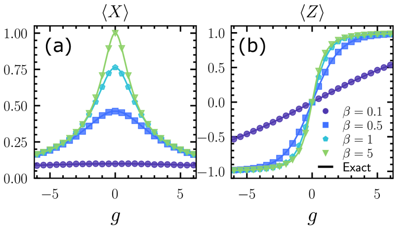
Figure 1: Sampling of a single spin. The magnetizations (a) $\braket{\hat{X}}$ and (b) $\braket{\hat{Z}}$ for the Hamiltonian Eq. (23), measured from trajectory sampling (data points) and compared to the exact result (solid lines) for various inverse temperatures $\beta$.

As an illustration of the ideas above, we consider a simple problem which will be important later in this paper: a single two-level system (which we will refer to as a spin), with the states $\sigma=\{-1,+1\}$.

A generic Hamiltonian for such a system reads

$$\hat{H}^{\rm spin}=-\hat{X}-g\hat{Z},$$ (23)

where $\hat{X}$, $\hat{Y}$ and $\hat{Z}$ are the usual Pauli operators. By calculating the matrix exponential of Eq. (23), is can be shown that the reduced dynamics, Eq. (15), takes the form

$$Z_{t}(\sigma_{i},\sigma_{f})=\begin{cases}\cosh(\theta_{t})+\frac{g}{\sqrt{1+g^{2}}}\sinh(\theta_{t}),&\sigma_{i,f}=1\\ \cosh(\theta_{t})-\frac{g}{\sqrt{1+g^{2}}}\sinh(\theta_{t}),&\sigma_{i,f}=-1\\ \frac{1}{\sqrt{1+g^{2}}}\sinh(\theta_{t}),&\sigma_{i}\neq\sigma_{f}\end{cases}$$ (24)

where $\theta_{t}=t\sqrt{1+g^{2}}$. Using Eq. (24), we are able to define a time-dependant stochastic dynamics which allows us to exactly sample trajectories with probabilities given by Eq. (7). The initial/final configuration $\sigma_{0}$ is chosen with probability ${Z_{\beta}(\sigma_{0},\sigma_{0})}/{\sum_{\sigma}Z_{\beta}(\sigma,\sigma)}$, and the time-dependent transition rates for the dynamics are

$$\tilde{K}_{\sigma\to-\sigma}(t;\beta,\sigma_{0})=\frac{Z_{\beta-t}(-\sigma,\sigma_{0})}{Z_{\beta-t}(\sigma,\sigma_{0})}.$$ (25)

By simply running this dynamics we sample the trajectories we need for computing thermal averages in this problem. The results are shown in Figs. 1(a, b) for the average magnetizations $\braket{\hat{X}}$ and $\braket{\hat{Z}}$ for various inverse temperatures $\beta$. The data points show the trajectory-averaged values using Eqs. (12) and (13). The numerical results coincide with the exact averages,

$$\braket{\hat{Z}}=g\braket{\hat{X}}=\frac{g}{\sqrt{1+g^{2}}}\tanh(\beta\sqrt{1+g^{2}}).$$ (26)

IV Transverse field Ising model in dimensions one and two

We now show how the trajectory sampling approach can be used to sample from the Boltzmann distribution of the transverse-field Ising model (TFIM) with $N$ spins

$$\hat{H} =-h\sum_{i=1}^{N}\hat{X}_{i}-J\sum_{\left<i,j\right>}\hat{Z}_{i}\hat{Z}_{j}$$ (27)

where $\hat{X}_{i}$ and $\hat{Z}_{i}$ are the Pauli operators acting on site $i$, and nearest neighbours are denoted by $\left<i,j\right>$. The method we use in this section can be equally adapted to accommodate for any other potential (the second summation) with the same single-body kinetic term. In the next section we demonstrate how to deal with other kinetic terms.

In what follows we set $h=1$ and consider periodic boundary conditions in space. Sampling directly from the full partition function Eq. (4) is difficult. We instead use a single-spin update scheme, whereby we update the entire trajectory for a single spin, keeping the trajectories of all other spins fixed by sampling directly from a reduced partition function.

IV.1 Redrawing trajectories for an individual spin

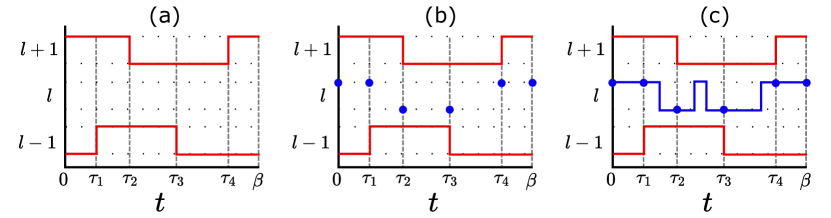
Figure 2: Single-spin update scheme for the 1D TFIM. The spin $l$ is updated while all the other spins are kept fixed. Only the spins $l-1$ and $l+1$ (red) contribute to the reduced Hamiltonian of the $l$-th spin. These spins change at the times $\tau_{m}$ (dashed grey lines). The update proceeds through the following steps: (a) The trajectory for spin $l$ is discarded. (b) We then sample the configurations $\tilde{\sigma}^{l}_{m}$ (blue circles) at the times in which the reduced Hamiltonian instantaneously changes, as explained. (c) We then sample bridges between each of the $\tilde{\sigma}^{l}_{m}$ to construct the full trajectory (blue line).

We now explain how our formulation can be used to perform single spin updates of the many-body trajectories. These updates adjust the entire trajectory of a single spin within the many-body trajectory, modelling the other spins as an effective time-dependent environment (or heat bath [17]). We stress that this update is equivalent to that presented in Ref. [17], which considered Eq. (27) on the Bethe lattice, and similarly that of Ref. [18] for the classical Ising model. Here, we instead use this approach on the TFIM in 1D and 2D to demonstrate how the update can be used to investigate the ground state properties and phase transitions of quantum lattice models.

IV.1.1 Factorization of the partition function

We consider the many-body trajectory ${\bm{\omega}}$ as a collection of the $N$ individual spin trajectories, ${\bm{\omega}}=\{{\bm{\sigma}^{1}},\cdots,{\bm{\sigma}^{N}}\}$, with ${\bm{\sigma}^{j}}$ denoting the time series of transitions for spin $j$

$${\bm{\sigma}^{j}}=\{(t^{j}_{0},\sigma^{j}_{0}),(t^{j}_{1},\sigma^{j}_{1}),\cdots,(t^{j}_{M_{j}},\sigma^{j}_{M_{j}})\},$$ (28)

each with a total of $M_{j}$ transitions. The partition function becomes

$$Z^{\rm TFIM}_{\beta}=\sum_{\{{\bm{\omega}}\}}\left[\prod_{i=1}^{N}\delta_{\sigma^{i}(0),\sigma^{i}(\beta)}\right]e^{\int_{0}^{\beta}dt\,\sum_{\braket{i,j}}J{\sigma}^{i}(t){\sigma}^{j}(t)}\\ \prod_{j=1}^{N}\prod_{m=1}^{\mathcal{K}\mkern-1.0mu({\bm{\sigma}}^{j})}K_{\sigma^{j}_{m-1}\to\sigma^{j}_{m}}.$$ (29)

In the above all $K_{\sigma\to\sigma^{\prime}}=1$, cf. Eq. (27), but we keep them in the expression to keep track of the spin transitions.

At this point, we notice that we are able to factorize Eq. (29) into a factor which depends on a specific ${\bm{\sigma}^{l}}$, and a factor which does not,

$$Z^{\rm TFIM}_{\beta}=\sum_{\{{\bm{\omega}}\}}\Bigg{(}\delta_{\sigma^{l}\mkern-1.0mu(0),\sigma^{l}\mkern-1.0mu(\beta)}\,e^{\int_{0}^{\beta}dt\,\sum_{i;\braket{i,l}}J{\sigma}^{i}\mkern-1.0mu(t)\mkern 1.5mu{\sigma}^{l}\mkern-1.5mu(t)}\prod_{m=1}^{\mathcal{K}\mkern-1.0mu({\bm{\sigma}}^{l})}K_{\sigma^{l}_{m-1}\to\sigma^{l}_{m}}\Bigg{)}\\ \prod_{p\neq l}\Bigg{(}\delta_{\sigma^{p}\mkern-1.0mu(0),\sigma^{p}\mkern-1.0mu(\beta)}\,e^{\int_{0}^{\beta}dt\,\frac{1}{2}\sum_{j\neq l;\braket{j,p}}J{\sigma}^{p}\mkern-1.0mu(t)\mkern 1.5mu{\sigma}^{j}\mkern-1.0mu(t)}\prod_{n=1}^{\mathcal{K}\mkern-1.0mu({\bm{\sigma}}^{p})}K_{\sigma^{p}_{n-1}\to\sigma^{p}_{n}}\Biggl{)},$$ (30)

where $\{i;\braket{i,l}\}$ denotes sites $i$ which are nearest neighbours of $l$, and $\{j\neq l;\braket{j,p}\}$ sites $j$ different from $l$ which are nearest neighbours of $p$.

We can now express Eq. (30) as a sum over each spin $l$ and for each $l$ over the partial trajectories

$${\bm{\sigma}}^{(l)}=\{{\bm{\sigma}^{1}},\cdots,{\bm{\sigma}^{l-1}},{\bm{\sigma}^{l+1}},\cdots{\bm{\sigma}^{N}}\},$$ (31)

that is, the individual trajectories of all the spins other than $l$. The first factor in Eq. (30) depends on the trajectory of the spin $l$ and its neighbouring spins through the interactions $\sum_{\braket{i,l}}J\sigma^{i}(t)\sigma^{l}(t)$, which we rewrite in the form of a time-dependent field

$$g^{l}(t):=g(t|{\bm{\sigma}}^{(l)})=\sum_{i;\braket{i,l}}J\sigma^{i}(t).$$ (32)

The second factor in Eq. (30) only depends on the trajectories of the spins $p\neq l$, and we denote it $\mathcal{N}({\bm{\sigma}}^{(l)})$. The partition function can now be written as

$$Z^{\rm TFIM}_{\beta}=N^{-1}\sum_{l}\sum_{\{{\bm{\sigma}}^{(l)}\}}\mathcal{N}({\bm{\sigma}}^{(l)})\,\sum_{\{{\bm{\sigma}}^{l}\}}\delta_{{\sigma^{l}}\mkern-1.0mu(0),{\sigma^{l}}\mkern-1.0mu(\beta)}\,e^{\int_{0}^{\beta}dt\,g^{l}\mkern-1.0mu(t)\mkern 1.5mu{\sigma}^{l}\mkern-1.0mu(t)}\,\prod_{m=1}^{\mathcal{K}\mkern-1.0mu({\bm{\sigma}}^{l})}K_{\sigma^{l}_{m-1}\to\sigma^{l}_{m}}.$$ (33)

The sum over $\{{\bm{\sigma}}^{l}\}$ is the same as the partition function of a single spin under a time-dependent longitudinal field, $g^{l}(t)$ , which we name $Z^{l}_{\beta}[g^{l}]$. This field is piecewise constant, meaning it remains constant except for a discrete number of times, $\tilde{M}$, when it instantaneously transitions to some other value. $\tilde{M}$ is decided by the sum of the number of times any of the neighbouring spins transition. This partition function takes the form

$$Z^{l}_{\beta}[g^{l}]=\sum_{\tilde{\sigma}^{l}_{0}}\braket{\tilde{\sigma}^{l}_{0}}{\prod_{m=0}^{\tilde{M}}\hat{U}^{l}_{m}\,}{\tilde{\sigma}^{l}_{0}},$$ (34)

with

$$\hat{U}^{l}_{m}=\exp\left[-(\tau_{m+1}-\tau_{m})\hat{H}^{l}_{m}\right],$$ (35)

and

$$\hat{H}^{l}_{m}=-\hat{X}^{l}-g^{l}\mkern-1.0mu(\tau_{m})\mkern 1.5mu\hat{Z}^{l}.$$ (36)

$\tau_{m}$ denote the times when the effective field $g^{l}(\tau)$ instantaneously changes, with $\tau_{0}=0$ and $\tau_{\tilde{M}+1}=\beta$. This is illustrated for the 1D TFIM in Fig. 2(a). The red lines show the trajectories of neighbouring spins in some partial trajectory, with the vertical dashed lines showing the times when the effective field $g$ changes. Notice that Eqs. (35) and (36) are nothing more than single-spin dynamics solved earlier in this paper, cf. Eq. (24).

IV.1.2 Sampling the edge configurations

While we have reduced the problem to one of a single spin, we still have the issue that the effective Hamiltonian for this spin is time-dependent. This is simple to deal with if we determine the configuration of the spin at each of the times the Hamiltonian changes instantaneously, $\tilde{\sigma}^{l}_{m}={\bm{\sigma}}^{l}(\tau_{m})$. Note that we use the tilde to denote the fact that $\tilde{\sigma}^{l}_{m}$ refers to the configuration of the spin when the effective Hamiltonian changes, which is different from the $\sigma^{l}_{m}$ used in Eq. (28) which is the configuration of spin $l$ after a given transition. By inserting the resolution of identity into Eq. (34), we find

$$Z^{l}_{\beta}[g^{l}]=\sum_{\tilde{\sigma}^{l}_{0},\cdots,{\tilde{\sigma}^{l}}_{\tilde{M}}}\prod_{m=0}^{\tilde{M}}\braket{\tilde{\sigma}^{l}_{m+1}}{\hat{U}^{l}_{m}}{\tilde{\sigma}^{l}_{m}},$$ (37)

with $\tilde{\sigma}^{l}_{\tilde{M}+1}=\tilde{\sigma}^{l}_{0}$.

The configurations $\tilde{\sigma}^{l}_{m}$ can be sampled sequentially. To this end, we define

$$P_{O}(\hat{O}_{0},\cdots,\hat{O}_{\tilde{M}})=\frac{1}{Z^{l}_{\beta}[g^{l}]}\operatorname{Tr}\left[\prod_{m=0}^{\tilde{M}}\hat{U}_{m}^{l}\hat{O}_{m}\right].$$ (38)

Then the probability of observing the sequence of configurations $\{\tilde{\sigma}^{l}_{m}\,|\,m=0,\dots,\tilde{M}\}$ is

$$P(\tilde{\sigma}^{l}_{0},\cdots,\tilde{\sigma}^{l}_{M})=P_{O}(\hat{\sigma}^{l}_{0},\cdots,\hat{\sigma}^{l}_{\tilde{M}}),$$ (39)

where $\hat{\sigma}^{l}_{m}=\ket{\tilde{\sigma}^{l}_{m}}\bra{\tilde{\sigma}^{l}_{m}}$. We first choose the initial/final configuration, $\tilde{\sigma}^{l}_{0}$, with probability $P(\tilde{\sigma}^{l}_{0})=P_{O}(\hat{\sigma}^{l}_{0},\hat{I},\cdots,\hat{I})$. The remaining $\tilde{\sigma}^{l}_{m}$ can be determined inductively using the conditional probabilities

$$P(\tilde{\sigma}^{l}_{m}\,|\,\{\tilde{\sigma}^{l}_{0},\cdots,\tilde{\sigma}^{l}_{m-1}\})=\\ \frac{P_{O}(\hat{\sigma}^{l}_{0},\cdots,\hat{\sigma}^{l}_{m-1},\hat{\sigma}^{l}_{m},\hat{I},\cdots,\hat{I})}{P_{O}(\hat{\sigma}^{l}_{0},\cdots,\hat{\sigma}^{l}_{m-1},\hat{I},\hat{I},\cdots,\hat{I})}.$$ (40)

This procedure is illustrated in Fig. 2(b).

IV.1.3 Sampling the full trajectory

After we have sampled the configurations $\tilde{\sigma}^{l}_{m}$, the partition function Eq. (34) reduces to

$$\prod_{m=0}^{\tilde{M}}\braket{\tilde{\sigma}^{l}_{m+1}}{\hat{U}^{l}_{m}}{\tilde{\sigma}^{l}_{m}}.$$ (41)

The terms inside the product are nothing else than the dynamics of Sec. III.4, see Eq. (24). Thus, we can sample their trajectories as was done previously for the two-level system. This indicates that the trajectory between times $\tau_{m}$ and $\tau_{m+1}$ is sampled from a dynamics initialized in configuration $\tilde{\sigma}^{l}_{m}$, with transition rates

$$\tilde{K}_{\sigma^{l}\to-\sigma^{l}}(t;\Delta\tau_{m},\tilde{\sigma}^{l}_{m+1})=\frac{Z^{l}_{\Delta\tau_{m}-t}(-\sigma^{l},\tilde{\sigma}^{l}_{m+1})}{Z^{l}_{\Delta\tau_{m}-t}(\sigma^{l},\tilde{\sigma}^{l}_{m+1})},$$ (42)

where $\Delta\tau_{m}=\tau_{m+1}-\tau_{m}$, and $Z^{l}_{\Delta\tau_{m}-t}(\sigma^{l},\tilde{\sigma}^{l}_{m+1})$ is defined using Eq. (24) with $g=g^{l}(\tau_{m})$. Concatenating the partial trajectories gives the fully sampled trajectory for the spin ${\bm{\sigma}}^{l}$, see Fig. 2(c).

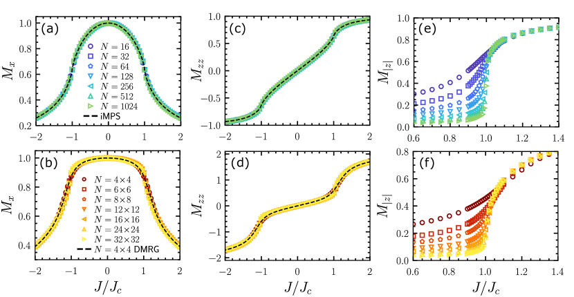
Figure 3: Ground state properties of the TFIM. Numerical results using the single-spin update for the 1D TFIM (top) for system sizes $N=\{16,32,64,128,256,512,1024\}$ and the 2D TFIM (bottom) with $N=L^{2}$ and $L=\{4,6,8,12,16,24,32\}$. We show the average transverse magnetization, $M_{x}$, in panels (a) and (b), the average two-spin correlator, $M_{zz}$, in panels (c) and (d) and the average magnetization, $M_{|z|},$ in panels (e) and (f). Data points are the results from trajectory sampling. The dashed black line in the top row of panels is from the iMPS, and from the 2D-DMRG with $L=4$ for the bottom row. The value of $J_{c}$ in 1D is $J_{c}=1$ and $J_{c}\approx 0.32747$ in 2D.

IV.2 Monte Carlo method

The method of resampling a trajectory for a single spin given in the previous section can now be used to implement a Monte Carlo algorithm to sample the many-body trajectories using the following steps:

1. Create some initial seed trajectory, ${\bm{\omega}}=({\bm{\sigma}}^{1},\cdots,{\bm{\sigma}}^{N})$ with inverse temperature $\beta$.

2. Choose a random lattice site $l\in[1,N]$.

3. Generate a new trajectory, ${\bm{\sigma}}^{l}$, for the spin.

4. Repeat from step 2 until convergence.

There are various ways to generate an initial seed trajectory. The key requirement is periodicity in the time interval $[0,\beta]$. The simplest way to achieve this is to generate the trajectory for each spin independently with a non-interacting dynamics, but allowing for the possibility of a local longitudinal field (see Sec. III.4). The choice of the initial trajectory can be guided by the phase one is trying to target. For example, for the TFIM with $J/h>1$ we expect to see ferromagnetic behaviour, and so we could choose a large local longitudinal field to force an initial trajectory with a higher likelihood of magnetic ordering. A second approach, which we discuss below is thermal annealing.

For $|J/h|>1$, there is spontaneous breaking of the symmetry at the level of the ground state. Indeed, depending on the initial trajectory seed, the single-spin update approach will break the $\mathbb{Z}_{2}$ symmetry and will only be ergodic over one of the ground states. In practice, one should randomly perform the global update ${\bm{\sigma}}^{i}(t)\to-{\bm{\sigma}}^{i}(t)$ for all spins simultaneously to ensure both states are explored. In order to investigate the effects of the local updates, we choose to not do this here.

IV.3 Continuous phase transition in the TFIM

We now demonstrate the effectiveness of our approach for the 1D and 2D TFIM. For fixed $h=1$, they are known to undergo a continuous phase transition at the critical point $J_{c}=1$ [35] and $J_{c}\approx 0.32747$ [36, 37], respectively. We investigate their ground state by using the previously described trajectory sampling algorithm with $\beta=128$ and a variety of system sizes, $N$. Figures 3(a, b) show the average transverse magnetization,

$$M_{x}=N^{-1}\sum_{i=1}^{N}\braket{\hat{X}_{i}},$$ (43)

in 1D and 2D, respectively, while Figs. 3(c, d) show the two-spin correlator,

$$M_{zz}=N^{-1}\sum_{\braket{i,j}}\braket{\hat{Z}_{i}\hat{Z}_{j}}.$$ (44)

For 1D, we compare our results for systems of size $N=16$ to $1024$ to those from infinite matrix product states (iMPS) [38, 39]. These methods allow us to determine the properties of the 1D chain to high accuracy. In particular, we also use the infinite time-evolving block decimation (iTEBD) method [38, 39]. For 2D, we show results for systems $N=4\times 4$ to $32\times 32$. These demonstrate agreement with the 2D density matrix renormalization group (DMRG) [40, 41, 42] for $N=4\times 4$ (dashed line).

The characterization of a continuous phase transition requires an order parameter which displays a discontinuous derivative at the critical point $J_{c}$ in the large system size limit. The commonly used order parameter for Ising models is the longitudinal magnetization,

$$M_{|z|}=N^{-1}\left\langle\left|\sum_{i=1}^{N}\hat{Z}_{i}\right|\right\rangle.$$ (45)

Figures 3(e, f) demonstrate a sharp increase for $M_{|z|}$ at the critical point, $J/J_{c}=1$.

IV.4 Trajectory autocorrelations

We now investigate the autocorrelation properties of the sampling dynamics using the single-spin update for the 1D and 2D TFIM. Under TPS we generate a Markov chain of trajectories, $\{{\bm{\omega}}_{0}\to{\bm{\omega}}_{1}\to\cdots\to{\bm{\omega}}_{N_{\rm traj}}\}$. In order to test the convergence to the target trajectory ensemble, cf. Eq. (7), we define the autocorrelation between two trajectories in the Markov chain separated by $\mu$ TPS updates,

$$\mathcal{C}({\bm{\omega}}_{\nu},{\bm{\omega}}_{\nu+\mu})=\frac{1}{\beta N}\sum_{j=1}^{N}\int_{0}^{\beta}d\tau\,\sigma^{j}_{\nu}(\tau)\,\sigma^{j}_{\nu+\mu}(\tau),$$ (46)

where $\sigma^{j}_{\nu}(\tau)$ indicates the value of the $j$-spin of the $\nu$-th trajectory at time $\tau$. The trajectory ensemble average can then be estimated from the Markov chain,

$$C_{\mu}=\frac{1}{N_{\rm traj}-\mu}\sum_{\nu=1}^{N_{\rm traj}-\mu}\frac{\mathcal{C}({\bm{\omega}}_{\nu},{\bm{\omega}}_{\nu+\mu})-\braket{\hat{Z}}^{2}}{1-\braket{\hat{Z}}^{2}},$$ (47)

where $\braket{\hat{Z}}$ is the equilibrium expectation value of $\hat{Z}_{i}$ (for any $i$). With the above definition, this autocorrelator is normalized to be $C_{0}=1$ and $C_{\infty}=0$ for $N_{\rm traj}\to\infty$. We show $C_{\mu}$ in Fig. 4 for $\mu/N\in[1,7]$, for (a) the 1D TFIM and (b) the 2D TFIM. Far from the critical point the trajectory autocorrelation function decays approximately exponentially. Near the critical point, this decay indicates that trajectories remain correlated even after a considerable number of TPS iterations. This is a manifestation of the expected slow down of Monte Carlo sampling near criticality at the level of trajectory sampling.

Figure 4: Convergence in the TFIM. The autocorrelation between trajectories $C_{\mu}$ for $\mu/N\in[1,7]$ over the range $J/J_{c}\in[0,2]$ for (a) the 1D TFIM with $N=\beta=128$ and (b) the 2D TFIM with $N=L^{2}$, $L=32$ and $\beta=128$.

V Quantum triangular plaquette model

We now show how the local update scheme can be generalized to models with more complex kinetic terms in their Hamiltonians. As a concrete example we consider the quantum triangular plaquette model (QTPM) [19, 20, 21, 22, 23, 24, 25], a generalization of the classical TPM studied in the context of glassy systems [26, 27, 28]. This is a model defined on a triangular lattice with interactions between a subset of the triangular plaquettes and a magnetic field transverse to them. We write the Hamiltonian of the QTPM as

$$\hat{H}=-h\sum_{\{i,j,k\}\in{\raisebox{-1.4pt}{$\triangle$}}}\hat{X}_{i}\hat{X}_{j}\hat{X}_{k}-J\sum_{i=1}^{N}\hat{Z}_{i},$$ (48)

where $\triangle$ indicates the upward pointing triangular plaquettes in the triangular lattice, see Fig. 5. We have chosen a representation of the QTPM where the interactions are off-diagonal in the classical basis and the magnetic field is longitudinal. This corresponds to the dual model of the usual QTPM.

Most numerical studies [19, 22, 24] indicate that the QTPM has a first-order quantum phase transition at $|J_{c}/h_{c}|=1$ between two distinct phases. In our recent paper, Ref. [24], we used the method presented in Sec. IV with single-spin updates on the Hamiltonian dual to Eq. (48). The aim of this section is to demonstrate how the update scheme can be adjusted to account for Hamiltonians like Eq. (48) using local updates which redraw the trajectories for multiple spins, rather than a single spin.

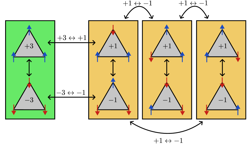
Figure 5: Elementary transitions in the TPM. A visualization of the allowed transitions in the TPM. A plaquette of three spins (spins are shown by blue / red arrows), $\triangle$, can flip. On the level of the individual plaquette, the plaquette can be in four different disconnected sectors, each containing two configurations and behaving like a two-level system. Within each sector, the system can move between the magnetizations $M_{\triangle}\leftrightarrow-M_{\triangle}$. The plaquettes in the green (left) box show plaquettes with total magnetization $M_{\triangle}=\pm 3$. The three orange boxes (right) show plaquettes with total magnetization $M_{\triangle}=\pm 1$. The flipping of a neighbouring plaquette, $\triangle^{\prime}$, causes a single spin within $\triangle$ to flip, moving $\triangle$ into a different sector, as demonstrated by the arrows connecting boxes. If it moves between the $M_{\triangle}=|3|$ and $M_{\triangle}=|1|$ sectors, then the sign of the magnetization $M_{\triangle}$ is preserved; otherwise, the sign is flipped.

V.1 Plaquette updates

The obvious Monte Carlo update is to randomly select a plaquette labelled by $\triangle$ encompassing three sites $\{i,j,k\}\in\triangle$. The trajectory of this plaquette is ${\bm{\eta}}^{\triangle}=\{{\bm{\sigma}}^{i},{\bm{\sigma}}^{j},\bm{\sigma}^{k}\}$. The corresponding transitions are those where the three spins in the plaquette flip simultaneously, in accordance with the kinetic term in Eq. (48). Given the eight different possible states of these three spins it might appear that one needs to consider this eight-level system in the simulations. However, as we will show below, what actually matters is the change in sign in the plaquette magnetization,

$$M_{\triangle}=\sigma^{i}+\sigma^{j}+\sigma^{k},$$ (49)

which reduces again the analysis to that of a local two-level system, see Fig. 5.

The time-dependent effective dynamics for the plaquette whose trajectory we choose to update is given by the six neighbouring plaquettes which contain any of the spins $i$, $j$ or $k$. Generalizing the approach used for the TFIM above, we do not modify the trajectories of these neighbouring plaquettes when updating plaquette $\triangle$. The neighbouring plaquettes will have $\tilde{M}$ flips at times $0\leq\tau_{1}\leq\tau_{2}\leq\cdots\leq\tau_{\tilde{M}}\leq\beta$. These transitions will force a single spin in $\eta^{\triangle}$ to flip at each of these times.

V.1.1 Factorization of the partition function

We start by writing the partition function as a sum over all possible imaginary-time trajectories,

$$Z^{\rm TPM}_{\beta}=\sum_{\{{\bm{\omega}}\}}e^{\sum_{i}\int_{0}^{\beta}dt\,J{\sigma}^{i}\mkern-1.0mu(t)}\prod_{\triangle}\prod_{m=1}^{\mathcal{K}\left({\bm{\eta}}^{\triangle}\right)}K_{\eta^{\triangle}_{m-1}\to\eta^{\triangle}_{m}},$$ (50)

where the plaquette trajectory is given by

$${\bm{\eta}}^{\triangle}=\{(t^{\triangle}_{0},\eta^{\triangle}_{0}),(t^{\triangle}_{1},\eta^{\triangle}_{1}),\cdots,(t^{\triangle}_{M},\eta^{\triangle}_{M})\},$$ (51)

and $K_{\eta^{\triangle}_{m-1}\to\eta^{\triangle}_{m}}$ denotes the corresponding plaquette flip.

As in the case of the TFIM, we can write Eq. (50) in a factorized form. Here, however, there will be three contributions. The first will contain all degrees of freedom and transitions within the plaquette $\triangle$. The second will contain all the transitions associated with the six other plaquettes that contain any of the spins $\{i,j,k\}\in\triangle$, and it will determine the effective dynamics for the plaquette $\triangle$. The third factor contains all other contributions which do not affect the dynamics of plaquette $\triangle$. The partition function reads

$$Z_{\beta}^{\rm TPM}=\sum_{\{{\bm{\omega}}\}}\left[e^{\sum_{i\in\triangle}\int_{0}^{\beta}dt\,J{\sigma}^{i}(t)}\prod_{m=1}^{\mathcal{K}\left({\bm{\eta}}^{\triangle}\right)}K_{\eta^{\triangle}_{m-1}\to\eta^{\triangle}_{m}}\right]\left[\prod_{{\triangle^{\prime}}}\prod_{m^{\prime}=1}^{\mathcal{K}\left({\bm{\eta}}^{\triangle^{\prime}}\right)}K_{\eta^{{\triangle^{\prime}}}_{m^{\prime}-1}\to\eta^{{\triangle^{\prime}}}_{m^{\prime}}}\right]\\ \left[e^{\sum_{i\not\in\triangle}\int_{0}^{\beta}dt\,J{\sigma}^{i}(t)}\prod_{{\triangle^{\prime\prime}}}\prod_{m^{\prime\prime}=1}^{\mathcal{K}\left({\bm{\eta}}^{\triangle^{\prime\prime}}\right)}K_{\eta^{{\triangle^{\prime\prime}}}_{m^{\prime\prime}-1}\to\eta^{{\triangle^{\prime\prime}}}_{m^{\prime\prime}}}\right],$$ (52)

where ${\triangle^{\prime}}$ labels the plaquettes which share a site with $\triangle$, and ${\triangle^{\prime\prime}}$ labels those which do not. The last factor does not depend on any of the spins within plaquette $\triangle$: as before, we denote ${\bm{\sigma}}^{(\triangle)}$ the trajectory of all the spins except from those $\{i,j,k\}\in\triangle$, and write this factor as $\mathcal{N}_{\triangle}\left({\bm{\sigma}}^{(\triangle)}\right)$. Since we can single out any of the $N$ plaquettes to write the partition sum as in Eq. (52), we can rewrite $Z^{\rm TPM}_{\beta}$ as a sum over all plaquettes and over all partial trajectories,

$$Z_{\beta}^{\rm TPM}=N^{-1}\sum_{{\triangle}}\sum_{\{{\bm{\sigma}}^{(\triangle)}\}}\mathcal{N}_{\triangle}\left({\bm{\sigma}}^{(\triangle)}\right)\left[e^{\sum_{i\in\triangle}\int_{0}^{\beta}dt\,J{\sigma}^{i}(t)}\prod_{m=1}^{\mathcal{K}\left({\bm{\eta}}^{\triangle}\right)}K_{\eta^{\triangle}_{m-1}\to\eta^{\triangle}_{m}}\right]\left[\prod_{\mkern 1.0mu\;{\triangle^{\prime}}}\prod_{m^{\prime}=1}^{\mathcal{K}\left({\bm{\eta}}^{\triangle^{\prime}}\right)}K_{\eta^{{\triangle^{\prime}}}_{m^{\prime}-1}\to\eta^{{\triangle^{\prime}}}_{m^{\prime}}}\right].$$ (53)

Now suppose we have a many-body trajectory which we wish to update. We randomly choose a plaquette $\triangle$ to update its trajectory ${\bm{\eta}}_{\triangle}$. The local partition function for the spins of the plaquette, $\{i,j,k\}\in\triangle$, is

$$Z^{\triangle}_{\beta}=\sum_{\eta_{0}}\braket{\eta_{0}}{\prod_{m=1}^{\tilde{M}}\hat{X}_{k_{m}}\hat{U}_{m}}{\eta_{0}},$$ (54)

where $\eta_{0}$ is the initial/final configuration of the plaquette, and $\hat{X}_{k_{m}}$ flips a spin $k_{m}$ in $\triangle$ due to the flipping of a neighbouring plaquette ${\triangle^{\prime}}$, where $k_{m}$ is determined entirely by which plaquette flips. The total number of times neighbouring plaquettes flip is given by $\tilde{M}$. The operator $\hat{U}_{m}$ is the time-evolution operator for the local plaquette,

$$\hat{U}_{m}=\exp\left[-(\tau_{m+1}-\tau_{m})\,\hat{H}_{m}\right],$$ (55)

where the Hamiltonian takes the form

$$\hat{H}_{m}=-\hat{X}_{i}\hat{X}_{j}\hat{X}_{k}-J(\hat{Z}_{i}+\hat{Z}_{j}+\hat{Z}_{k}).$$ (56)

The objective is to sample exactly a trajectory for each plaquette $\triangle$ from Eq. (54).

V.1.2 Determining the trajectory sector and sampling the trajectory

An important point to notice is that the trajectory space of ${\bm{\eta}}^{\triangle}$, for some chosen $\triangle$, is composed of four disconnected sectors, which we refer to as the trajectory sectors. An initial plaquette configuration $\eta^{\triangle}_{0}=\{\sigma^{i}_{0},\sigma^{j}_{0},\sigma^{k}_{0}\}$ will belong to one of the four local sectors shown in Fig. 5. At the times $\tau_{m}$ when there is a transition in a neighbouring plaquette ${\triangle^{\prime}}$, the sector of the plaquette $\triangle$ will transition into one of the other three sectors, as shown in Fig. 5; however, the sector it moves to is entirely determined by which plaquette ${\triangle^{\prime}}$ transitioned. Thus, the initial sector for $\eta_{0}$ will predetermine which local sector the plaquette will occupy at any time.

This observation implies that the local plaquette effectively behaves as a two-level (rather than an eight-level) system, and the flipping of neighbouring plaquettes at times $t_{m}$ changes the energies of the two levels according to the rules shown in Fig. 5. This allows us to solve Eq. (54) through the evolution of four separate two-level systems, which is computationally easier than solving the original eight-level system, by making use of the results in Sec. II. To determine the trajectory sector the plaquette will lie in, we must first calculate Eq. (54) for all four sectors, and use this as a weighting to randomly select one of the four sectors. Then, we can sample the edge configurations before and after each time $\tau_{m}$, as was done in Sec. IV. The sampling of the trajectory between $\tau_{m}$ and $\tau_{m+1}$ is then performed by using the methods of Sec. II.

V.2 Thermal annealing

The expected first-order phase transition at $J_{c}$ can slow down the convergence for $J\approx J_{c}$ and large inverse temperatures, $\beta$. In particular, if the initial seed trajectory is chosen to be in one of the two phases, there is the possibility that the update procedure cannot explore the entire trajectory space, thus remaining stuck in the incorrect phase. This is a consequence of the large barriers which need to be overcome to move between phases. Furthermore, making assumptions on which phase the trajectory should belong to a priori for some value of $J$ could bias the results.

A common technique used in Monte Carlo sampling to overcome such metastability is thermal annealing. In this approach, we start from a small inverse temperature (we use $\beta=0.1$) and gradually increase it to the target inverse temperature ($\beta=128$ in our case). Our annealing schedule is to make $N$ updates to the trajectory and then increase $\beta$ by $\Delta\beta=0.1$ for $\beta<32$, and $\Delta\beta=1$ for $\beta\geq 32$. When the inverse temperature is increased, we have to modify the trajectory to account for this. In practice, we just stretch the trajectory time as $\beta\leftarrow(\beta+\delta\beta)/\beta$. After reaching the target inverse temperature, we do $N\times 10^{2}$ updates, and then restart the process. We repeat this procedure $10^{3}$ times.

We find this approach to work well. Indeed, when sufficiently far from $J=1$, the generated trajectories (at the target dynamics) have behaviour corresponding to their correct phase with high accuracy. However, when close to $J=1$, the trajectories can have properties which correspond to either phase (in practice, we find that the process picks just one of the phases for each run of the annealing process). While we cannot be certain this approach guarantees the correct amount of mixing between the phases, it provides a less biased way to propose initial trajectory seeds, and still demonstrates the first-order behaviour of the transition point.

V.3 First-order quantum phase transition of the QTPM

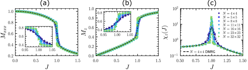
Figure 6: Ground state phase transition in the QTPM. Results using TPS with exact plaquette updates and simulated annealing for $N=L\times L$ and $L=\{4,5,8,11,16,23,32\}$. We show (a) the three spin correlator, $M_{xxx}$, (b) the longitudinal magnetization, $M_{z}$ and (c) the magnetic susceptibility, $\chi_{z}(J)=dM_{z}/dJ$. The data points show results from trajectory sampling, and for comparison, the dashed lines show results from DMRG for $N=4\times 4$. The insets show the behaviour close to the transition point.

We now demonstrate how the plaquette update scheme with temperature annealing can be used to investigate the quantum phase transition of the QTPM. As described in Ref. [24], the finite size study of the QTPM has to be done with care, since, depending on the size and aspect ratio of the system used, Eq. (48) can have many or no symmetries. We focus on square lattices $N=L\times L$, with $L=\{4,5,8,11,16,23,32\}$ chosen such that there are no such symmetries [24]. We also compare our results against those from 2D DMRG for $N=4\times 4$.

Figure. 6(a) shows the average transverse three-spin correlator,

$$M_{xxx}=N^{-1}\sum_{\{i,j,k\}\in{\raisebox{-1.4pt}{$\triangle$}}}\braket{\hat{X}_{i}\hat{X}_{j}\hat{X}_{k}}.$$ (57)

The inset shows the results close to the transition point. Figure 6(b) shows the average longitudinal magnetization,

$$M_{z}=N^{-1}\sum_{i=1}^{N}\braket{\hat{Z}_{i}}.$$ (58)

As we increase the system size, the crossover between the two phases becomes increasingly step-like, suggesting a first-order singularity in the large size limit. The behaviour of the magnetic susceptibility,

$$\chi_{Z}(J)=\frac{dM_{z}}{dJ},$$ (59)

is consistent with this interpretation, with its peak getting higher and narrower around $J=1$ with the system size, see Fig. 6(c).

VI Conclusions

In this paper we have leveraged the connection between the continuous-time expansion of the quantum Boltzmann distribution and the rare-event sampling in stochastic dynamics. In particular, for quantum systems with no sign problem (so-called stoquastic Hamiltonians), computing the partition sum is equivalent to sampling atypical imaginary-time trajectories of a continuous-time Markov chain, where the trajectories are conditioned to return to the initial configuration, and their probability is exponentially biased (or tilted) due to the difference between the Hamiltonian and the associated stochastic generator. Such atypical trajectories can be accessed with a method like TPS, i.e. Monte Carlo for trajectory ensembles. Specifically, we showed that in systems with finite-state local degrees of freedom (such as spins on a lattice) one can use an approach similar to that of Refs. [17, 18] to devise a rejection-free TPS scheme, by means of an exact local generation of trajectory updates which is especially simple in spin-$1/2$ models. In fact, as we showed above, this gives the optimal, or Doob, dynamics for sampling the rare trajectories.

We illustrated the effectiveness of this approach studying the quantum phase transitions of two classes of models. The first was the TFIM in 1D and 2D, where the transition is well known to be continuous. We showed that the rejection-free TPS method correctly characterizes the quantum phase transition of the TFIM, even in the near-critical regime where trajectories take many TPS iterations to decorrelate. The second class of models we considered are quantum plaquette models. In particular, we studied the QTPM, and showed how to generalize the rejection-free method to local multi-spin updates. While less understood than the TFIM, the QTPM has a quantum phase transition which is first-order. Again, the rejection-free method efficiently recovered the quantum phase transition. As a by-product we also computed to high accuracy the statistics of dynamical observables (both in the large deviation regime and for finite imaginary times) in the trajectory ensembles that resolve the quantum partition sums of both the TFIM and the QTPM, which is shown in Appendix B.

While the method we used here is based on local updates, the key property is not locality but simplicity, which allows the sampling of exact trajectory moves by solving Eqs. (21) and (22) that define the Doob dynamics. It would be interesting to find other (perhaps non-local) moves that also solve Eqs. (21) and (22). While finding exact updates might prove difficult, one might be able to formulate an approximately optimal dynamics, with the error accounted for in an acceptance test, such as Metropolis in a TPS scheme. The difficulty here is finding a dynamics which provides improvements in sampling while defined in terms of transition rates which remain computationally cheap (perhaps building on the use of tensor networks for optimal sampling [43]).

Data and code availability

The data shown in the figures is available at Ref. [44]. Example code used to generate the data can be found at https://github.com/lcauser/ctqmc-tps.

Appendix A Sampling time-dependant optimal dynamics

Suppose we are able to resolve the optimal dynamics given in Sec. III.3, with the transition rates given by Eq. (21). This is a time-dependant dynamics which is defined through the reduced dynamics Eq. (15). To sample dynamics from it, we follow the process drawn out in Sec. III.2, which requires randomly drawing waiting times from the distribution Eq. (17), and then randomly selecting a configuration to jump to from the distribution Eq. (18).

Determining a random transition time, $\tau$, is easily done by considering the cumulative distibution function of Eq. (17),

$$C_{x}(\tau;\beta,x_{\rm f},t)=1-\exp\left[-\int_{t}^{t+\tau}dt^{\prime}\,\tilde{R}_{x}(t^{\prime};\beta,x_{\rm f})\right].$$ (60)

It is well understood that by drawing some uniformly random number $r\in[0,1]$, and inverting $C_{x}(\tau;\beta,x_{\rm f},t)=r$, one can pick $\tau$ with a probability density given by Eq. (17). Using Eq. (22), we find

$$C_{x}(\tau;\beta,x_{\rm f},t)=1-\frac{Z_{\beta-t-\tau}(x;x_{\rm f})}{Z_{\beta-t}(x;x_{\rm f})}e^{-\tau H_{x}^{c}}.$$ (61)

While analtically inverting Eq. (61) is difficult, it can be done numerically to arbitary accuracy using the bisection method if one is able to calculate $Z_{t}(x;x_{\rm f})$. This is due to the fact $C_{x}(\tau;\beta,x_{f},t)$ is a monotonically increasing function between $C_{x}(0;\beta,x_{\rm f},t)=0$ and $C_{x}(\beta-t;\beta,x_{\rm f},t)<1$. Note that if $r>C_{x}(\beta-t;\beta,x_{\rm f},t)$, then no transition time is drawn, and the system remains in state $x$ until the terminating trajectory time, $\beta$.

Once a transition time, $\tau$, has been drawn, the state which the system transitions to can be determined using Eq. (18),

$$P_{x}(y\,|\,t+\tau;\beta,x_{\rm f})=\frac{K_{x\to y}\,Z_{\beta-t-\tau}(y;x_{\rm f})}{\sum_{z\neq x}K_{x\to z}\,Z_{\beta-t-\tau}(z;x_{\rm f})}.$$ (62)

Appendix B Trajectory statistics

The connection between the quantum partition function and the ensemble of (conditioned/biased) stochastic trajectories naturally motivates the investigation of the trajectory statistics of the imaginary-time dynamics. Given some trajectory ensemble, such as one defined by Eq. (7), and some inverse temperature (or trajectory time), $\beta$, we can define its probability distribution function over a trajectory observable, ${\cal O}({\bm{x}})$, through

$$P_{\beta}({\cal O})=\sum_{\{{\bm{x}}\}}\pi({\bm{x}})\delta\left[{\cal O}({\bm{x}})-{\cal O}\right].$$ (63)

For simplicity, we will only consider trajectory observables which are obtained by time integrating diagonal operators,

$${\cal O}({\bm{x}})=\int_{0}^{\beta}dt\,O({x}(t)).$$ (64)

In practice, the computation of Eq. (63) for some arbitrary inverse temperature $\beta$ is difficult. However, in the low temperature limit, $\beta\to\infty$, one can estimate Eq. (63) using the framework of large deviation (LD) theory (for reviews, see e.g. Refs. [45, 46, 47, 48]).

In the low temperature limit both the probability distribution of ${\cal O}$ and its moment generating function (MGF),

$$Z_{\beta}(s)=\sum_{\{{\bm{x}}\}}P_{\beta}({\bm{x}})\,e^{-s{\cal O}({\bm{x}})},$$ (65)

take the LD forms

$$P_{\beta}({\cal O})\asymp e^{-\beta\varphi({\cal O}/\beta)},\;\;\;Z_{\beta}(s)\asymp e^{\beta\theta(s)},$$ (66)

respectively. Here, $\varphi$ is the rate function, and $\theta$ is the scaled cumulant generating function (SCGF), with the two related through the Legendre transform, $\theta(s)=-\min_{o}\left[s{o}+\varphi(o)\right]$, where $o=\mathcal{O}/\beta$.

The MGF has a form similar to the partition function, Eq. (3). In terms of trajectories it reads, cf. Eq. (4),

$$Z_{\beta}(s) =\sum_{\{{\bm{x}}\}}P_{\beta}({\bm{x}})e^{-s\int_{0}^{\beta}dt\,O({{x}(t))}}$$ (67)

$$=\frac{1}{Z_{\beta}}\sum_{\{{\bm{x}}\}}\delta_{{x}(0),{x}(\beta)}e^{-\int_{0}^{\beta}dt\,[H^{\rm c}_{{\bm{x}}(t)}+s\,O({x}(t))]}$$

$$\phantom{xxxxxxx}\prod_{m=1}^{\mathcal{K}({\bm{x}})}K_{x_{m-1}\to x_{m}}.$$ (68)

Furthermore, from Eq. (68) we also see that the MGF can be written as

$$Z_{\beta}(s)=\frac{\operatorname{Tr}[e^{-\beta\hat{H}_{s}}]}{Z_{\beta}},$$ (69)

where $\hat{H}_{s}$ is a tilting [45] of the original Hamiltonian,

$$\hat{H}_{s}=\hat{H}+s\hat{O}.$$ (70)

This means that in the limit of small temperatures, Eq. (66), we get that $\theta(s)=E_{s}-E$, where $E_{s}$ is the ground state energy of $\hat{H}_{s}$ and $E$ that of $\hat{H}_{s=0}=\hat{H}$. For the following we use this to connect quantum phase transitions to transitions in the LD statistics of trajectory observables.

B.1 TFIM

Figure 7: Dynamical fluctuations of the imaginary-time trajectories of the 2D TFIM. The low-temperature trajectory statistics are encoded in the dynamical LDs. We show the rate function, $-\varphi({\mathcal{M}}_{zz}/\beta)/N$, for the two-point correlator, $M_{zz}$, for (a) $J/J_{c}=1.0$, (b) $J/J_{c}=0.5$, and (c) $J/J_{c}=1.5$. The data points show results from trajectory sampling with $\beta=128$. The dashed line shows the 2D DMRG for $N=4\times 4$. (d) Rate function $-\varphi({\mathcal{M}}_{|z|}/\beta)/N$ for $J/J_{c}=1.0$ and $\beta=64$. The dotted line shows the rate function for the time-integral of the longitudinal magnetization of a single spin from Eq. (23), with $\braket{\hat{\sigma}^{z}}=0.45$.

We first use the methods of Sec. IV to investigate the trajectory statistics of the TFIM in 2D. The first trajectory observable we consider, cf. Eq. (64), is the time integral of the two-point correlator,

$${\mathcal{M}}_{zz}({\bm{\omega}})=\int_{0}^{\beta}d\tau\sum_{\langle i,j\rangle}{\sigma}^{i}(\tau)\,{\sigma}^{j}(\tau).$$ (71)

We focus on the low-temperature limit, $\beta\gg 1$, corresponding to the ground state behaviour, where LD theory can be applied. The LD statistics are retrieved from the ground state properties of the tilted Hamiltonian,

$$\hat{H}_{s}=-h\sum_{i}\hat{X}_{i}-(J-s)\sum_{\left<i,j\right>}\hat{Z}_{i}\hat{Z}_{j},$$ (72)

which is the same as the original Hamiltonian with $J\to J-s$. Figure 7 shows the rate function, $-\varphi({\mathcal{M}}_{zz}/\beta)$, c.f. Eq. (66), for the 2D TFIM with (a) $J/J_{c}=1$, (b) $J/J_{c}=0.5$ and (c) $J/J_{c}=1.5$. At criticality, we observe a broadening in this distribution, demonstrating the divergence in correlation lengths. In contrast, away from the critical point the distributions become narrower.

The second trajectory quantity we consider is the time-integral of the order parameter,

$${\mathcal{M}}_{|z|}(\bm{\omega})=\int_{0}^{\beta}d\tau\left|\sum_{i=1}^{N}{\sigma}^{i}(\tau)\right|.$$ (73)

The corresponding tilted Hamiltonian is

$$\hat{H}_{s}=-h\sum_{i}\hat{X}_{i}-J\sum_{\left<i,j\right>}\hat{Z}_{i}\hat{Z}_{j}+s\left|\sum_{i=1}^{N}\hat{Z}_{i}\right|.$$ (74)

To simulate dynamics with Eq. (74), we can use the single-spin update scheme previously described, but we must now consider the trajectories of all other spins when constructing the time-dependent dynamics, due to the coupling introduced via $M_{|z|}$ in Eq. (74). While this makes the procedure more costly, we are still able to run dynamics for moderate $N$. We show the rate function in Fig. 7(d). Here, the broadening at criticality is more pronounced; for comparison, we show the rate function for the longitudinal magnetization of a single spin (dashed line). This broadening suggests a diverging magnetic susceptibility in the large size limit.

B.2 QTPM

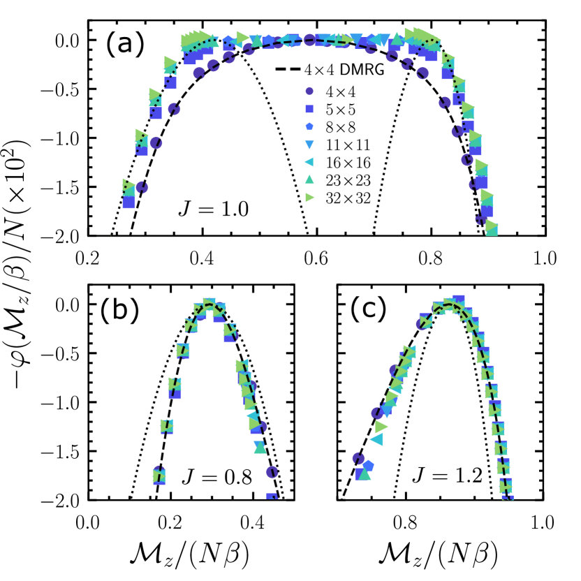
Figure 8: Large deviations in the long imaginary-time trajectories of the QTPM. The long imaginary-time trajectory statistics can be captured through the LDs. We show the rate function, $-\varphi({\mathcal{M}}_{z})/N$, for (a) $J=1.0$, (b) $J=0.8$ and (c) $J=1.2$. The data points show results from trajectory sampling for $N=L\times L$ with $L=\{4,5,8,11,16,23,32\}$, and the dashed line from 2D DMRG for $L=4$. For comparison, the dotted lines show the rate functions for the single spin Eq. (23) case, where $g$ is chosen to fit the mean to the peak of the QTPM distributions.

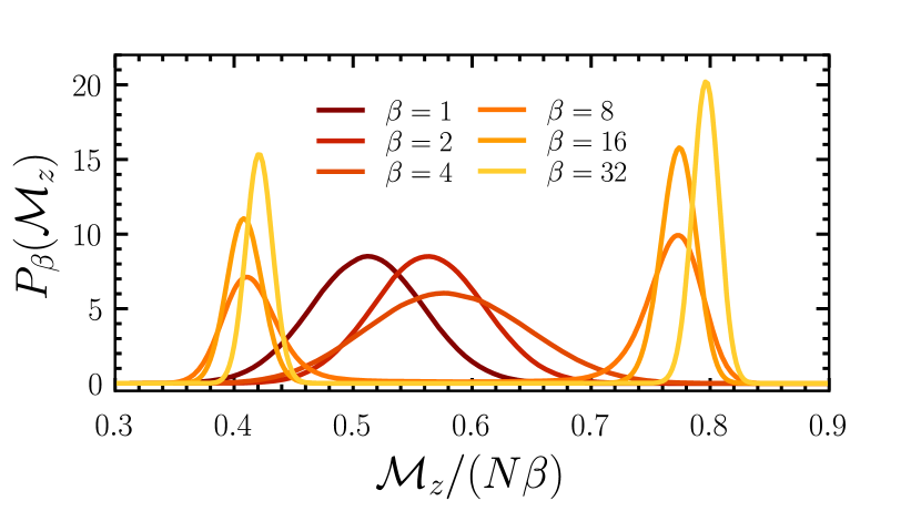
Figure 9: Trajectory statistics at finite imaginary times in the QTPM. The estimated distribution of the time-integrated magnetization for $L=16$ for various finite times (inverse temperatures) at $J=1$ from trajectory sampling. The lines are calculated using a Gaussian kernel with $\delta=0.005$.

We now investigate the effects of the first-order phase transition of the QTPM at the level of the imaginary-time trajectories. We consider the statistics of the trajectory observable

$${\mathcal{M}}_{z}({\bm{\omega}})=\int_{0}^{\beta}d\tau\sum_{i=1}^{N}\sigma^{i}(\tau)$$ (75)

They are encoded in the tilted Hamiltonian,

$$\hat{H}_{s}=-h\sum_{\{i,j,k\}\,\in{\raisebox{-1.4pt}{$\triangle$}}}\hat{X}_{i}\hat{X}_{j}\hat{X}_{k}-(J-s)\sum_{i=1}^{N}\hat{Z}_{i},$$ (76)

which corresponds to the original Hamiltonian with $J\to J-s$. Figure 8 shows the rate function $-\varphi({\mathcal{M}}_{z}/\beta)$ for various $J$. The rate function at $J_{c}$ is shown in Fig. 8(a): the rate function flattens with increasing system size, indicating the existence of large fluctuations. This behaviour is characteristic of a (dynamical) first-order phase transition due to the coexistence of two distinct (dynamical) phases. For comparison we show the LDs of the single-spin problem from Eq. (23) (dotted lines), where the value of $g$ is chosen to fix the mean of the distribution. Figure 8(a) shows the LDs of the single-spin problem with $\braket{M_{z}}=0.42$ and $0.8$, which approximately match the tails of the distribution for the QTPM. The interpretation is clear: the two coexisting phases are homogeneous phases of distinct ${\mathcal{M}}_{z}$, and intra-phase fluctuations are uninteresting (thus the modes are well approximated by a single spin); the broadening in $\varphi$ in the QTPM is due to a Maxwell construction between these modes due to the fact that intermediate values of ${\mathcal{M}}_{z}$ are realised by coexistence, i.e. space-time regions of one phase separated by sharp interfaces from space-time regions of the other phase. In Figs. 8(b) and (c) we also show the rate functions away from the transition point for $J=\{0.8,1.2\}$, respectively. While here there is a slight broadening in the tails, these distributions describe single phases far from coexistence.

It is also possible to reasonably estimate the probability distribution $P_{\beta}({\mathcal{M}}_{z})$ for finite $\beta$ (that is finite imaginary times) through sampling. This is shown in Fig. 9 at the transition point for $N=16$, for various inverse temperatures. We use our annealing strategy to sample $N_{\rm traj}=10^{6}$ trajectories for each inverse temperature. The results are used to approximate the probability distribution function using the Gaussian kernel,

$$P_{\beta}(\mathcal{M}_{z})\approx\mathcal{N}\sum_{i=1}^{N_{\rm traj}}\exp\left(-\frac{[\mathcal{M}_{z}-\mathcal{M}_{z}({\bm{\omega}}^{i})]^{2}}{2\delta^{2}}\right),$$ (77)

where $\mathcal{N}$ is a normalization constant, $\mathcal{M}_{z}({\bm{\omega}}^{i})$ is the time-integrated magnetization of the $i$-th trajectory, and $\delta=0.005$ is the width of the filter. Notice that at small inverse temperatures the distribution looks approximately Gaussian. However, with increasing $\beta$, the distribution becomes bimodal, demonstrating explicitly the coexistence of phases.

References

- Metropolis et al. [1953] N. Metropolis, A. W. Rosenbluth, M. N. Rosenbluth, A. H. Teller, and E. Teller, J. Chem. Phys 21, 1087 (1953).
- Hastings [1970] W. K. Hastings, Biometrika 57, 97 (1970).
- Glauber [1963] R. J. Glauber, J. Math. Phys 4, 294 (1963).
- Sandvik [2019] A. W. Sandvik, Chapter 16 of Many-Body Methods for Real Materials, Vol. 9 (2019).
- Suzuki et al. [1977] M. Suzuki, S. Miyashita, and A. Kuroda, Prog. Theor. Phys 58, 1377 (1977).
- Hirsch et al. [1982] J. E. Hirsch, R. L. Sugar, D. J. Scalapino, and R. Blankenbecler, Phys. Rev. B 26, 5033 (1982).
- Beard and Wiese [1996] B. B. Beard and U.-J. Wiese, Phys. Rev. Lett. 77, 5130 (1996).
- Prokof’ev et al. [1998] N. V. Prokof’ev, B. V. Svistunov, and I. S. Tupitsyn, J. Exp. Theor. Phys 87, 310 (1998).
- Rubtsov et al. [2005] A. N. Rubtsov, V. V. Savkin, and A. I. Lichtenstein, Phys. Rev. B 72, 035122 (2005).
- Gull et al. [2011] E. Gull, A. J. Millis, A. I. Lichtenstein, A. N. Rubtsov, M. Troyer, and P. Werner, Rev. Mod. Phys. 83, 349 (2011).
- Note [1] Another approach worth mentioning is the stochastic series expansion (e.g. Refs. [49, 50, 51, 52, 4]), which instead utilises the Taylor expansion of the exponential in order to obtain strings of operators. While this does not require the consideration of imaginary time, there is still an added complexity in the length of the strings of operators.
- Loh et al. [1990] E. Y. Loh, J. E. Gubernatis, R. T. Scalettar, S. R. White, D. J. Scalapino, and R. L. Sugar, Phys. Rev. B 41, 9301 (1990).
- Pan and Meng [2022] G. Pan and Z. Y. Meng, arXiv: 2204.08777 (2022).
- Jack and Sollich [2010] R. L. Jack and P. Sollich, Prog. Theor. Phys. Supp. 184, 304 (2010).
- Chetrite and Touchette [2015] R. Chetrite and H. Touchette, Ann. Henri Poincaré 16, 2005 (2015).
- Garrahan [2016] J. P. Garrahan, J. Stat. Mech.: Theory Exp 2016, 073208 (2016).
- Krzakala et al. [2008] F. Krzakala, A. Rosso, G. Semerjian, and F. Zamponi, Phys. Rev. B 78, 134428 (2008).
- Mora et al. [2012] T. Mora, A. M. Walczak, and F. Zamponi, Phys. Rev. E 85, 036710 (2012).
- Yoshida and Kubica [2014] B. Yoshida and A. Kubica, arXiv:1404.6311 (2014).
- Devakul [2019] T. Devakul, Phys. Rev. B 99, 235131 (2019).
- Devakul et al. [2019] T. Devakul, Y. You, F. J. Burnell, and S. L. Sondhi, SciPost Phys. 6, 007 (2019).
- Vasiloiu et al. [2020] L. M. Vasiloiu, T. H. E. Oakes, F. Carollo, and J. P. Garrahan, Phys. Rev. E 101, 042115 (2020).
- Zhou et al. [2021] Z. Zhou, X.-F. Zhang, F. Pollmann, and Y. You, arXiv:2105.05851 (2021).
- Sfairopoulos et al. [2023] K. Sfairopoulos, L. Causer, J. F. Mair, and J. P. Garrahan, arXiv:2301.02826 (2023).
- Wiedmann et al. [2023] R. Wiedmann, L. Lenke., M. Mühlhauser, and K. P. Schmidt, arXiv: 2302.01773 (2023).
- Newman and Moore [1999] M. E. J. Newman and C. Moore, Phys. Rev. E 60, 5068 (1999).
- Garrahan and Newman [2000] J. P. Garrahan and M. E. J. Newman, Phys. Rev. E 62, 7670 (2000).
- Garrahan [2002] J. P. Garrahan, J. Phys.: Condens. Matter 14, 1571 (2002).
- Dyson [1949] F. J. Dyson, Phys. Rev. 75, 486 (1949).
- Bolhuis et al. [2002] P. G. Bolhuis, D. Chandler, C. Dellago, and P. L. Geissler, Annu. Rev. Phys. Chem. 53, 291 (2002).
- Dellago et al. [2006] C. Dellago, P. Bolhuis, and P. Geissler, Transition path sampling methods, in Computer Simulations in Condensed Matter Systems: From Materials to Chemical Biology Volume 1 (Springer Berlin Heidelberg, Berlin, Heidelberg, 2006) pp. 349–391.
- Bortz et al. [1975] A. Bortz, M. Kalos, and J. Lebowitz, J. Comput. Phys 17, 10 (1975).
- Gillespie [1976] D. T. Gillespie, J. Comput. Phys 22, 403 (1976).
- Gillespie [1977] D. T. Gillespie, J. Phys. Chem. 81, 2340 (1977).
- Sachdev [2011] S. Sachdev, Quantum Phase Transitions, 2nd ed. (Cambridge University Press, 2011).
- Rieger and Kawashima [1999] H. Rieger and N. Kawashima, Eur. Phys. J. B 9, 233 (1999).
- Blöte and Deng [2002] H. W. J. Blöte and Y. Deng, Phys. Rev. E 66, 066110 (2002).
- Vidal [2007] G. Vidal, Phys. Rev. Lett. 98, 070201 (2007).
- Orús and Vidal [2008] R. Orús and G. Vidal, Phys. Rev. B 78, 155117 (2008).
- White [1992] S. R. White, Phys. Rev. Lett. 69, 2863 (1992).
- Schollwöck [2011] U. Schollwöck, Ann. Phys. 326, 96 (2011).
- Stoudenmire and White [2012] E. Stoudenmire and S. R. White, Annu. Rev. Condens. Matter Phys. 3, 111 (2012).
- Causer et al. [2023a] L. Causer, M. C. Bañuls, and J. P. Garrahan, Phys. Rev. Lett. 130, 147401 (2023a).
- Causer et al. [2023b] L. Causer, K. Sfairopoulos, J. F. Mair, and J. Garrahan, Data for ”Rejection-free quantum Monte Carlo in continuous time from transition path sampling” (2023b).
- Touchette [2009] H. Touchette, Phys. Rep 478, 1 (2009).
- Garrahan [2018] J. P. Garrahan, Physica A 504, 130 (2018).
- Jack [2020] R. L. Jack, Eur. Phys. J. B 93, 74 (2020).
- Limmer et al. [2021] D. T. Limmer, C. Y. Gao, and A. R. Poggioli, Eur. Phys. J. B 94, 145 (2021).
- Handscomb [1964] D. C. Handscomb, Math. Proc. Camb. Philos. Soc 60, 115 (1964).
- Sandvik and Kurkijärvi [1991] A. W. Sandvik and J. Kurkijärvi, Phys. Rev. B 43, 5950 (1991).
- Sandvik [1992] A. W. Sandvik, J. Phys. A 25, 3667 (1992).
- Syljuåsen and Sandvik [2002] O. F. Syljuåsen and A. W. Sandvik, Phys. Rev. E 66, 046701 (2002).