Quantum Monte Carlo for Gauge Fields and Matter without the Fermion Determinant

Abstract

Ab-initio Monte Carlo simulations of strongly-interacting fermionic systems are plagued by the fermion sign problem, making the non-perturbative study of many interesting regimes of dense quantum matter, or of theories of odd numbers of fermion flavors, challenging. Moreover, typical fermion algorithms require the computation (or sampling) of the fermion determinant. We focus instead on the meron cluster algorithm, which can solve the fermion sign problem in a class of models without involving the determinant. We develop and benchmark new meron algorithms to simulate fermions coupled to $\mathbb{Z}_{2}$ and $U(1)$ gauge fields to uncover potential exotic properties of matter, particularly relevant for quantum simulator experiments. We demonstrate the emergence of the Gauss’ Law at low temperatures for a $U(1)$ model in $(1+1)-$d.

Introduction.–

Microscopic models involving fermions that strongly interact with each other, either directly or mediated via gauge fields, are essential ingredients of many theories in condensed matter and particle physics [1, 2, 3]. From the Hubbard model describing the physics of correlated fermions, to the quantum Hall effect and high-temperature superconductivity, fermions subjected to various interactions have been studied both perturbatively and non-perturbatively [4, 5]. Fermions constitute the matter component of all microscopic theories of particle physics (as leptons in electromagnetic and weak interactions, as quarks in strong interactions) and interact with gauge fields (the photon, the $W^{\pm},Z$, and the gluons respectively) [6]. Gauge fields are also becoming increasingly important to condensed matter systems, from frustrated magnetism to theories of deconfined quantum criticality [7].

While Quantum Monte Carlo (QMC) methods are robust for non-perturbative studies of the aforementioned systems, they are also vulnerable to the sign problem [8]. QMC methods work by performing importance sampling of fermion and gauge field configurations that make up the partition function. Since fermions anti-commute, their sign problem can be straightforwardly understood when the configurations considered are worldlines: whenever fermions exchange positions an odd number of times, the configuration weight acquires another negative sign factor, leading to huge cancellations in the summation, accompanied by an exponential increase of noise [9].

A large family of QMC methods deal with the fermion sign problem using determinants: they introduce auxiliary bosonic fields and integrate out the fermions, or expand the partition function, ${\cal Z}$, as powers of the Hamiltonian (or parts of the Hamiltonian) and get fermion determinants for the resulting terms [10, 11]. Because these methods result in weights that are the sums of many worldline configurations, they can be used more generically to simulate the largest classes of sign-problem-free Hamiltonians, with Auxiliary Field QMC as the most widely applicable method [12, 13, 14, 15, 16, 17, 18, 19, 20]. Determinantal methods in general scale with either the spatial lattice volume, or the spacetime lattice volume, which in terms of imaginary time $\beta$ and spatial lattice dimension $N$ goes either as $O(\beta^{3}N^{3})$ or $O(\beta N^{3})$, depending on the method [21, 22, 23, 24, 25, 26]. While this polynomial scaling is much better than the exponential scaling from a straightforward exact diagonalization (ED), it is much worse than the linear scaling achievable for spin systems, where worldline-based methods can simulate systems orders of magnitude larger than typical simulable fermionic systems [27, 28, 29, 30, 31, 32].

An alternative approach–well-utilized in the lattice quantum chromodynamics (LQCD) community, is the Hybrid Monte Carlo technique [33, 34, 35], which computes the fermion determinant stochastically, and theoretically scales linearly rather than cubicly with the spatial volume. For systems of massless fermions and thus zero modes in ${\cal Z}$, however, the method can run into complexities and the scaling significantly worsens, closer to the cubic scaling of before [36]. More recently, it has been applied to problems in condensed matter with some promising optimizations [37, 38, 39].

It is however possible to develop worldline-based algorithms for fermionic Hamiltonians [40, 41, 42, 43]. The meron cluster method [44] as devised for four-fermion Hamiltonians is an example, and for certain parameters it can be applied in a sign-problem-free way to spin-polarized interacting fermions, as well as free fermions with a chemical potential [45]. Because these methods sample worldlines, computing the weights scales linearly with the volume of the system, and negative terms in the partition function are taken care of by avoiding merons — this is what distinguishes them from bosonic simulations. The relative simplicity of this method, with each weight corresponding to a worldline configuration and the lack of stabilization issues that can arise in determinantal methods [11], as well as the favorable scaling of the weight computations, makes it an attractive choice for simulation when applicable. Correspondingly, exciting opportunities open up when new interesting physical models are found which can be simulated using this method [46, 47, 48].

Recently, there has been intense experimental development to study the physics of confinement and quantum spin liquids [49, 50, 51, 52, 53, 54, 55] using tools of quantum simulation and computation. The microscopic models used to capture the physics involve fermions interacting with (Abelian) gauge fields. In this Letter, we develop meron cluster algorithms for a class of experimentally relevant models [56, 57], enabling a robust elucidation of their phase diagrams. We also introduce new classes of $\mathbb{Z}_{2}$ and $U(1)$ multi-flavored gauge-fermion theories, which might be realized in cold-atom setups and also be further studied using Monte Carlo techniques. Notably, the $U(1)$ family of these models seems to be one of the few families that falls outside the class of models known to be simulable by auxiliary-field methods, as are [23, 58, 59]. Moreover, due to the worldline nature of the method, this can be easily employed to study the corresponding phases in these theories in higher spatial dimensions.

Models

– The $\mathbb{Z}_{2}$- and $U(1)$-symmetric model families involve the following terms inspired by the $t$-$V$ model with $V=2t>0$, which was found to be simulable by meron clusters [45, 48]:

$$H^{(g)}_{N_{f}}=-\sum_{\left\langle xy\right\rangle}\prod_{f=1}^{N_{f}}\left(H^{(g)}_{\left\langle xy\right\rangle,f}+H^{(g),\mathrm{des}}_{\left\langle xy\right\rangle,f}\right)$$ (1)

The label $g\in\left\{U(1),\mathbb{Z}_{2}\right\}$ is the gauge symmetry, and the first term is given by

$$H^{\mathbb{Z}_{2}}_{\left\langle xy\right\rangle,f} =t\left(c^{\dagger}_{x,f}s^{1}_{xy,f}c_{y,f}+c^{\dagger}_{y,f}s^{1}_{xy,f}c_{x,f}\right)$$ (2)

$$H^{U(1)}_{\left\langle xy\right\rangle,f} =t\left(c^{\dagger}_{x,f}s^{+}_{xy,f}c_{y,f}+c^{\dagger}_{y,f}s^{-}_{xy,f}c_{x,f}\right).$$

Then $H^{(g),\mathrm{des}}_{\left\langle xy\right\rangle,f}$ is a designer term[60] that makes the models particularly amenable to the Meron cluster algorithm,

$$H^{\mathbb{Z}_{2},\mathrm{des}}_{\left\langle xy\right\rangle,f} =-2t\left(n_{x,f}-\frac{1}{2}\right)\left(n_{y,f}-\frac{1}{2}\right)+\frac{t}{2}$$ (3)

$$H^{U(1),\mathrm{des}}_{\left\langle xy\right\rangle,f} =-t\left(n_{x,f}-\frac{1}{2}\right)\left(n_{y,f}-\frac{1}{2}\right)$$

$$\qquad\qquad\quad-ts_{xy,f}^{3}\left(n_{y,f}-n_{x,f}\right)+\frac{t}{4}$$

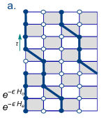
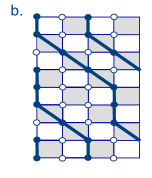
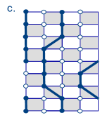
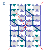
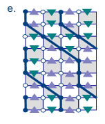
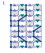
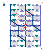
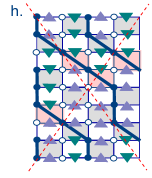
Figure 1: Worldlines for the $t$-$V$ model are in (a)-(c), the $\mathbb{Z}_{2}$ theory in (d)-(f), and the $U(1)$ theory in (g)-(i). Image (a) shows the imaginary time direction and the $(1+1)$-d trotterization, which is the same for all images.

These terms are here for similar reasons that the $V=2t$ term must be included for the meron cluster algorithm applied to the $t$-$V$ model[45], and similarly an additional particle-hole symmetric $V$ term can be added to the models here in a sign-problem-free way. For the $\mathbb{Z}_{2}$ gauge theory, the Pauli matrix, $s^{1}=\sigma^{1}/2$ couples to fermions, and one can see the local $\mathbb{Z}_{2}$ symmetry from the operator $Q_{x}$, which commutes with the $H^{\mathbb{Z}_{2}}$ and is given by $Q_{x}=(-1)^{\sum_{f}n_{x,f}}\prod_{f,\hat{\alpha}}s^{3}_{x,x+\hat{\alpha},f}s^{3}_{x-\hat{\alpha},x,f}$, where $\hat{\alpha}$ are the unit vectors in a $d$-dimensional square lattice. For the $U(1)$ theory, one can see the $U(1)$ symmetry from the unitary operator $V_{U(1)}$ which commutes with $H^{U(1)}$ and is given by $V_{U(1)}=\prod_{x}e^{i\theta_{x}G_{x}}$, with $G_{x}=\sum_{f}\left[n_{x,f}-\sum_{\hat{\alpha}}\left(s^{3}_{x,x+\hat{\alpha},f}-s^{3}_{x-\hat{\alpha},x,f}\right)\right]$. In the terminology of gauge fields, our microscopic models are quantum link models [61], which realize the continuous gauge invariance using finite=dimensional quantum degrees of freedom. The identification with usual gauge field operators is $U_{xy,f}=s^{+}_{xy,f},~{}U^{\dagger}_{xy,f}=s^{-}_{xy,f},E=s^{3}_{xy,f}$. We note that a straightforward application of the meron idea necessitates the introduction of an equivalent flavor index for gauge links as fermion flavors. Naively, the total Gauss law can be expressed through a product ($\mathbb{Z}_{2}$) or sum ($U(1)$) of the Gauss law of individual flavors degrees of freedom, and the resulting theories have $\mathbb{Z}_{2}^{\otimes N_{f}}$ and $U(1)^{\otimes N_{f}}$ gauge symmetry. However, flavored gauge-interactions can also be turned on in the $U(1)$ model (as explained in the Supplementary Material),

$$H^{U\left(1\right)}_{N_{f}=2}\rightarrow H^{U\left(1\right)}_{N_{f}=2}+J\sum_{\left\langle xy\right\rangle}s^{3}_{xy,1}s^{3}_{xy,2},$$ (4)

or through a Hubbard-U interaction for both $\mathbb{Z}_{2}$ and $U(1)$-symmetric models [48]. These additions would directly cause ordering for either the gauge field or the fermions, and the coupling between them leads to the interesting question of how the other particles are affected by this ordering. In similar contexts, interesting simultaneous phase transitions of both the fermions and gauge fields have been found [47, 62, 63, 64, 65, 66, 67].

Algorithm

– To understand the algorithm, we first consider the possible worldline configurations for the base models defined in Eqs. 1, 2 and 3. The occupation number basis for the fermions and the electric flux (spin-$z$) basis for the gauge links is used for the time evolution of a Fock state. The partition function in $(1+1)$-d is then

$${\cal Z}={\mathrm{Tr}}\left(e^{-\beta H}\right)$$ (5)

$$\;=\sum_{\left\{s,n\right\}}\left\langle s_{1},n_{1}\right|e^{-\epsilon H_{e}}\left|s_{2N_{t}},n_{2N_{t}}\right\rangle\left\langle s_{2N_{t}},n_{2N_{t}}\right|$$

$$\qquad\times e^{-\epsilon H_{o}}...e^{-\epsilon H_{e}}\left|s_{2},n_{2}\right\rangle\left\langle s_{2},n_{2}\right|e^{-\epsilon H_{o}}\left|s_{1},n_{1}\right\rangle,$$

where $H=H_{e}+H_{o}$, and $H_{e}$ ($H_{o}$) consists of Hamiltonian terms that correspond to even (odd) links. This is a Trotterized approximation, and all terms within $H_{e}$ and $H_{o}$ commute with each other (there are straightforward generalizations for higher dimensions) [68]. We thus have a sum of terms that consist of discrete time-slices $1,\cdots,2N_{t}$, each with defined electric flux and fermion occupation numbers for each of the time-slices. Each of the terms in Eq. 5 is a worldline configuration, and the rules for allowable worldline configurations apply consistently to all of our models within each of the symmetry families. Fig. 1(a)-(c) give examples of such configurations for the $t$-$V$ model as simulated by meron clusters.

In the $\mathbb{Z}_{2}$ case, for each time-slice a fermion has the option of hopping to an unoccupied nearest neighbor site of the same flavor. If the fermion hops, then the electric flux on the bond between the nearest neighbor sites that shares the same fermion flavor index must also flip–this is the result of the $s_{xy}^{1}$ operator. Fig. 1(d)-(f) gives example configurations for the $N_{f}=1$ version of this model. Due to the trace condition, it is impossible to have odd winding numbers because these would cause the spins in the initial state to not match the spins in the final state.

The possible worldline configurations for the $U(1)$ are similar to the $\mathbb{Z}_{2}$ case, but more restrictive. The $s^{+}_{xy}$ and $s^{-}_{xy}$ operators allow the hopping for a given flavor of fermion only in one direction or the other for each bond, depending on the orientation of the same flavored flux on the bond. Fig. 1(g)-(i) illustrates an example configuration and restrictions for the single flavor version of the $U(1)$ model. In $(1+1)$-d, it is clear that all allowed configurations must have zero winding number.

The worldline configurations are a tool to obtain meron cluster configurations by introducing appropriate breakups, which decompose the terms in Eq. 5 into further constituents. In considering the allowed worldline configurations given in Fig. 1 for the $U(1)$ theory, for example, each of the active plaquettes in each time-slice (shaded in gray) must be one of the plaquettes given in Table 1. The plaquettes in each row share the same weight, computed using $\left\langle s_{b},n_{b}\right|e^{-\epsilon H_{b}}\left|s_{b}^{\prime},n_{b}^{\prime}\right\rangle$, from Eq. 5, where $b$ is a nearest neighbor bond, $b=\{x,y\}$. The corresponding breakup cell for each row gives allowable breakups: if all fermion occupations/spins are flipped along any one of the lines, the resulting plaquette also exists in this table. From the table, we see two such breakups are defined, $A$ and $D$. By computing the matrix elements that correspond to the plaquettes in each grouping, we find that for the $U(1)$ theory, the corresponding breakup weights $w_{A}$ and $w_{D}$ must obey:

$$w_{A} =1$$ (6)

$$w_{D} =\exp\left(\epsilon t\right)\sinh\epsilon t$$

$$w_{A}+w_{D} =\exp\left(\epsilon t\right)\cosh\epsilon t,$$

Plaquettes	Breakups

Table 1: Plaquettes and breakups for the $U(1)$-symmetric Hamiltonian.

to satisfy detailed balance. Moreover, the choice of the breakups is such that the total sign of a configuration factorizes into a product of the signs of each cluster: Sign $\left[C\right]$ = $\prod_{i}^{N_{c}}$ Sign$\left[C_{i}\right]$, where the configuration $C$ has been decomposed into $N_{c}$ clusters. We can thus simulate this system similarly to the simulation of the $t$-$V$ model at $V=2t$ [45], by exploring a configuration space where each configuration is defined according to the combination of worldlines and breakups. By assigning breakups to all active plaquettes, clusters are formed, and then updates involve flipping all fluxes and fermions within a cluster, which physically corresponds to generating a new worldline configuration. The algorithm begins with putting the system in a reference configuration, where the weight is known to be positive, and it is known that all other possible configurations can immediately be returned to the fermion portion of this configuration by choosing a subset of the clusters in a given configuration to flip. For both the $U(1)$ and $\mathbb{Z}_{2}$ theories, the reference configuration has a staggered occupation (charge density wave, or CDW) of fermions, where fermions and fluxes are stationary throughout imaginary time. Fluxes can be in any spatial configuration (because they do not contribute a sign), and the breakups are all $A$. A QMC sweep is then organized as follows:

1. Go through the list of the active plaquettes and update each breakup, one at a time.

   1. If the breakup can be changed for a plaquette, change it with probability dependent on the breakup weights.

   2. If the breakup is changed, consider the new configuration that would result from this change. If it contains a cluster where flipping the fermion occupation causes the fermions to permute in a way that produces a negative sign, then it is a meron. In that case, restore the breakup back to its initial state. Rules for identifying merons are given in [45, 69].

2. Identify the new clusters formed by the breakups in the new configuration. For each cluster, flip all fermions and fluxes with probability $1/2$.

This describes sampling of the zero-meron sector only, but sectors with other numbers of merons may become relevant depending on the observable. [45] We note that the cluster rules implement the Hamiltonian dynamics, but the constraints due to Gauss’ law are not included.

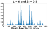
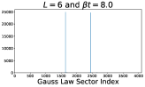
Figure 2: The number of configurations versus the sector (each of the sectors is given an index) for $50000$ equilibrated configurations. Two Gauss’ law sectors emerge at low temperature: $G_{x}=0$ and $G_{x}=(-1)^{x}$.

Numerical Results

– To illustrate the efficacy of the algorithm, we discuss results obtained by simulating the $(1+1)$-d $H^{U(1)}_{N_{f}=1}$ model in Eq. 1, which is related to the massless quantum-link Schwinger model [57, 70] and the PXP model [71, 72], where quantum scars were first demonstrated experimentally [50]. We simulate the model for different temperatures $\beta=1/T$, without imposing Gauss’ law. The one-dimensional nature of the problem forbids the presence of merons, providing a technical simplification. The first non-trivial result is the emergence of two Gauss’ law sectors at low temperatures, as shown in Fig. 2. For the $\mathbb{Z}_{2}$ theory in $(1+1)$-d, this result was also observed in [66] using the worm algorithm.

Generating different Gauss’ Law sectors has the benefit that the physics in each sector can be easily studied by applying a filter. At low temperatures, this is an ${\cal O}(1)$ effort, but becomes exponentially difficult at higher temperatures, since exponentially many sectors will be populated. Hence we note that the efficiency of this meron algorithm for true gauge theories (where Gauss’ law is imposed) is more suited to the study of quantum phase transitions rather than finite-temperature ones. For theories where multiple non-trivial Gauss’ Law sectors emerge at low temperature, it is possible to study the physics in all sectors without any extra effort.

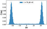
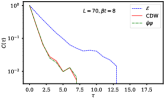
Figure 3: (left) The probability distribution of $\bar{\psi}\psi$, with peaks from the two emergent Gauss’ Law sectors, indicating that the algorithm efficiently samples all sectors that emerge at low temperatures. (right) The autocorrelation functions for different operators.

Similar to the well-studied Schwinger model [73, 74, 75, 76, 77, 78, 79], our model has the following discrete global symmetries: $\mathbb{Z}_{2}$ chiral symmetry, charge conjugation, $C$, and parity, $P$, [57], whose breaking depends on the strength of the four Fermi coupling. The order parameter sensitive to the $P$ or the $C$ symmetry is the total electric flux, ${\cal E}=\frac{1}{L_{t}}\sum_{x,t}s^{3}_{x,x+1}$, while the one for $\mathbb{Z}_{2}$ chiral symmetry is the chiral condensate, $\bar{\psi}\psi=\sum_{x}(-1)^{x}n_{x}$. In Fig. 3 (left) we show the probability distribution for $\bar{\psi}\psi$, which samples the two vaccua very well, and indicating that at $T=0$ the symmetry is spontaneously broken. We use these operators to check the algorithm against exact diagonalization results, as well as explore other features of the phase at low temperatures. We leave these discussions to the Supplementary Material, since the physics is well-understood, and instead concentrate on the performance of the meron algorithm measured via the autocorrelation function:

$$C_{\cal O}(\tau)=\frac{\braket{({\cal O}(i)-\overline{\cal O})({\cal O}(i+\tau)-\overline{\cal O})}}{\braket{({\cal O}(i)-\overline{\cal O})^{2}}},$$ (7)

where ${\cal O}(i)$ is the measured value at the $i$-th step of the appropriate operator (whose average is $\overline{\cal O}$), and is the running index summed over the MC data, while the autocorrelations are measured $\tau$ steps apart. Fig. 3 (right) shows the $C_{\cal O}(\tau)$ for three different operators: ${\cal E}$, $\bar{\psi}\psi$, and ${\rm CDW}$. We note that the order parameter ${\cal E}$ relaxes the slowest, while both the fermionic operators relax faster. Even for the slowest relaxing mode, the autocorrelation decreases by more than an order of magnitude within 10 MC steps for the largest lattice at the lowest temperature, demonstrating the efficiency of the algorithm. Finally, we also show the behaviour of the normalized susceptibilities corresponding to ${\cal E}$ and the CDW operator as a function of temperature for smaller lattices up to $L=22$ in the $G_{x}=0$ sector. While they converge to their zero temperature values relatively quickly as a function of the volume, we are also able to capture the finite temperature crossover.

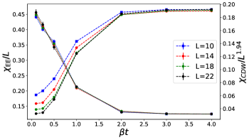
Figure 4: Finite temperature data for $U(1)$ theory in $1+1$-$d$. The dotted lines show the $\chi_{EE}$, which is the susceptibility corresponding to ${\cal E}$. This value rapidly converges to 0.125. On the other hand, the dashed lines trace the $\chi_{CDW}$ which display somewhat more finite size effects. The thermal behaviour of both observables indicate that the transition from low to high temperature is associated with a smooth crossover, consistent with the literature.

Conclusions

– In this paper, we have generalized the construction of the meron algorithm to cases where staggered fermions are coupled to quantum link gauge fields. This construction of the Monte Carlo algorithm is agnostic to the space-time dimension, and paves the way for ab-initio studies of large scale gauge-fermionic system with odd or even numbers of fermionic flavours, and includes models not simulable using DQMC. While we are able to simulate low temperatures at fixed values of gauge coupling by using two breakups, $A$ and $D$, it is possible to add different microscopic terms by increasing the allowed ways of bonding the fermions and gauge links. We have also indicated how to include multiple flavours, and multi-flavour interactions.

Our investigations open up avenues to study quantum link gauge theories coupled to fermions in higher dimensions, which are almost certain to exhibit quantum phase transitions. Since the physics of Abelian gauge fields represented by half-integer spins are sometimes related to quantum field theories at $\theta=\pi$ [80], where $\theta$ is the topological angle, our numerical method also promises to increase our knowledge of quantum field theories with non-trivial topologies. Our methods can be extended to gauge fields with larger spin representation, and hopefully to non-Abelian gauge fields as well, to tackle realistic interacting systems of increasing complexity in particle and condensed matter physics.

Acknowledgments

We would like to thank Joao Pinto Barros, Shailesh Chandrasekharan and Uwe-Jens Wiese for illuminating discussions and helpful comments. Research of EH at the Perimeter Institute is supported in part by the Government of Canada through the Department of Innovation, Science and Economic Development and by the Province of Ontario through the Ministry of Colleges and Universities. This work used Bridges 2 at the Pittsburgh Supercomputing Center through allocation PHY170036 from the Advanced Cyberinfrastructure Coordination Ecosystem: Services & Support (ACCESS) program, which is supported by National Science Foundation grants #2138259, #2138286, #2138307, #2137603, and #2138296.

Appendix A Supplementary Material

A.1 $\mathbb{Z}_{2}$-Symmetric Algorithm

The breakups for the $\mathbb{Z}_{2}$-symmetric model defined in Eq. 1 and Eq. 2 are given in Table 2. Their weights must satisfy the same equations as for the $U(1)$ theory,

$$w_{A} =1$$ (8)

$$w_{D} =\exp\left(\epsilon t\right)\sinh\epsilon t$$

$$w_{A}+w_{D} =\exp\left(\epsilon t\right)\cosh\epsilon t,$$

which are consistent and solved. The key difference is that more plaquettes are allowed for the $\mathbb{Z}_{2}$ theory compared to the $U(1)$ theory, as seen in the Table 2.

The algorithm then proceeds the same way described in the main text. Note that there are the same number and types of breakups, and their weights are the same as for a simulation of the $t$-$V$ model. The key difference for the gauge theory is that the $A$-breakup involves an additional vertical spin line. This causes clusters rather than loops to be formed, which constrain the types of fermionic worldlines that are allowed compared to the loops.

Plaquettes	Breakups

Table 2: Plaquettes and breakups for the $\mathbb{Z}_{2}$-symmetric Hamiltonian.

A.2 More than One Layer of Fermions and Spins

As mentioned in the main text of the paper, the models in (Eq. 1) are sign-problem-free and the meron cluster method applies to them. The weights of the matrix elements for one layer of the $U(1)$ model were shown explicitly. Here we give the weights for the $N_{f}$-layer model for the $U(1)$ theory and $\mathbb{Z}_{2}$ theory explicitly so that it is clear that they also are sign-problem-free and amenable to the meron cluster method.

First, for $N_{f}=1$ of the discrete-time version $U(1)$ theory, we can write out the matrix elements for a single bond as

$$e^{\epsilon t\left(\left[\sigma^{1}+\mathbbm{1}\right]_{2}\oplus\left[0\right]_{6}\right)}$$ (9)

$$\qquad=\left[\left(\frac{1}{2}e^{2\epsilon t}+\frac{1}{2}\right)\mathbbm{1}+\left(\frac{1}{2}e^{2\epsilon t}-\frac{1}{2}\right)\sigma^{1}\right]_{2}\oplus\mathbbm{1}_{6}.$$

These expressions for the diagonal and off-diagonal matrix elements in the $2\times 2$ space are the $e^{\epsilon t}\cosh(\epsilon t)$ and $e^{\epsilon t}\sinh(\epsilon t)$ from the main text, and because

$$1+\left(\frac{1}{2}e^{2\epsilon t}-\frac{1}{2}\right)=\left(\frac{1}{2}e^{2\epsilon t}+\frac{1}{2}\right)$$ (10)

we are able to use the $A$ and $D$ breakups to simulate the system.

This mathematical form for the weights is more obviously generalizable to the $N_{f}$-flavor version of the $U(1)$ theory, where the matrix elements for a bond are

$$\exp\left\{\epsilon t^{N_{f}}\left(\left[\left(\sigma^{1}+\mathbbm{1}\right)^{\otimes N_{f}}\right]_{m}\oplus\left[0\right]_{n}\right)\right\},$$ (11)

where $m=2^{N_{f}}$ and $n=2^{3N_{f}}-2^{N_{f}}$, performing the exponentiation then yields

$$\left[\left(\frac{1}{2^{N_{f}}}e^{\epsilon(2t)^{N_{f}}}+\left(1-\frac{1}{2^{N_{f}}}\right)\right)\mathbbm{1}_{m}\right.$$ (12)

$$\left.+\left(\frac{1}{2^{N_{f}}}e^{\epsilon(2t)^{N_{f}}}-\frac{1}{2^{N_{f}}}\right)O^{U(1)}_{m}\right]\oplus\mathbbm{1}_{n},$$

where we define $O^{U(1)}_{m}$ to be an “off-diagonal” matrix for the $U(1)$ theory, which is $m\times m$ and has entries of $1$ everywhere except for on the diagonal, where the entries are zero.

As required all weights are positive, and we have

$$1+\left(\frac{1}{2^{N_{f}}}e^{\epsilon(2t)^{N_{f}}}-\frac{1}{2^{N_{f}}}\right)$$ (13)

$$=\left(\frac{1}{2^{N_{f}}}e^{\epsilon(2t)^{N_{f}}}+\left(1-\frac{1}{2^{N_{f}}}\right)\right),$$

allowing us to use $A^{\otimes N_{f}}$ and $D^{\otimes N_{f}}$ breakups to simulate the system.

The $\mathbbm{Z}_{2}$ matrix elements are found from

$$\exp\big{\{}\epsilon t^{N_{f}}\left(\left[\left(\left(\sigma^{1}+\mathbbm{1}\right)\oplus\left(\sigma^{1}+\mathbbm{1}\right)\right)^{\otimes N_{f}}\right]_{m}\right.$$ (14)

$$\qquad\quad\qquad\qquad\qquad\qquad\qquad\qquad\qquad\left.\oplus\left[0\right]_{n}\right)\big{\}},$$

where this time $m=2^{2N_{f}}$ and $n=2^{3N_{f}}-2^{2N_{f}}$. Performing the exponentiation then yields

$$\left[\left(\frac{1}{2^{N_{f}}}e^{\epsilon(2t)^{N_{f}}}+\left(1-\frac{1}{2^{N_{f}}}\right)\right)\mathbbm{1}_{m}\right.$$ (15)

$$\left.+\left(\frac{1}{2^{N_{f}}}e^{\epsilon(2t)^{N_{f}}}-\frac{1}{2^{N_{f}}}\right)O_{m}^{\mathbb{Z}_{2}}\right]\oplus\mathbbm{1}_{n},$$

where the off-diagonal $O_{m}^{\mathbb{Z}_{2}}$ matrix is defined as

$$O_{m}^{\mathbb{Z}_{2}}=\left[\left(\sigma^{1}+1\right)\oplus\left(\sigma^{1}+1\right)\right]^{\otimes N_{f}}-\mathbbm{1}_{m},$$ (16)

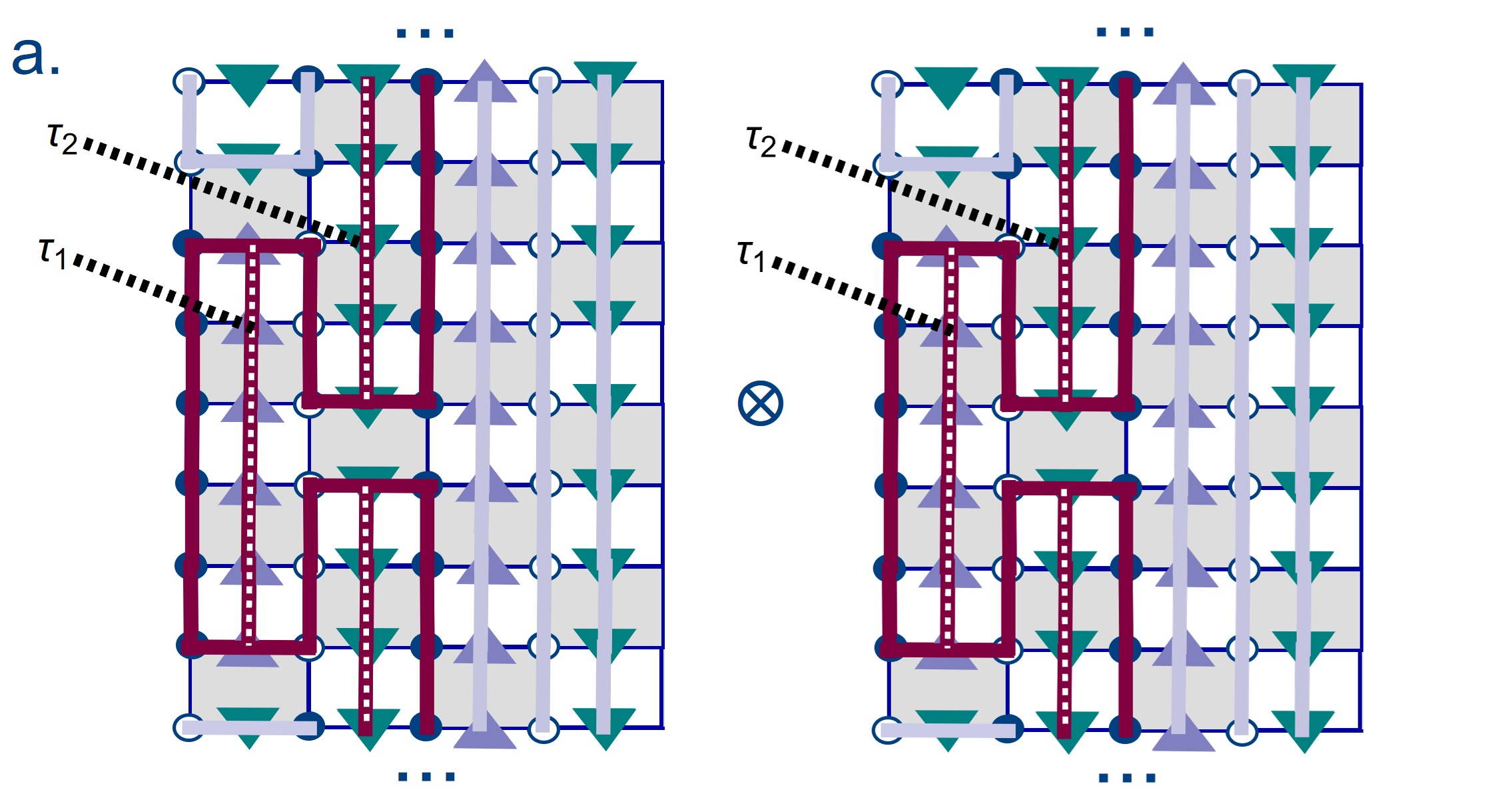
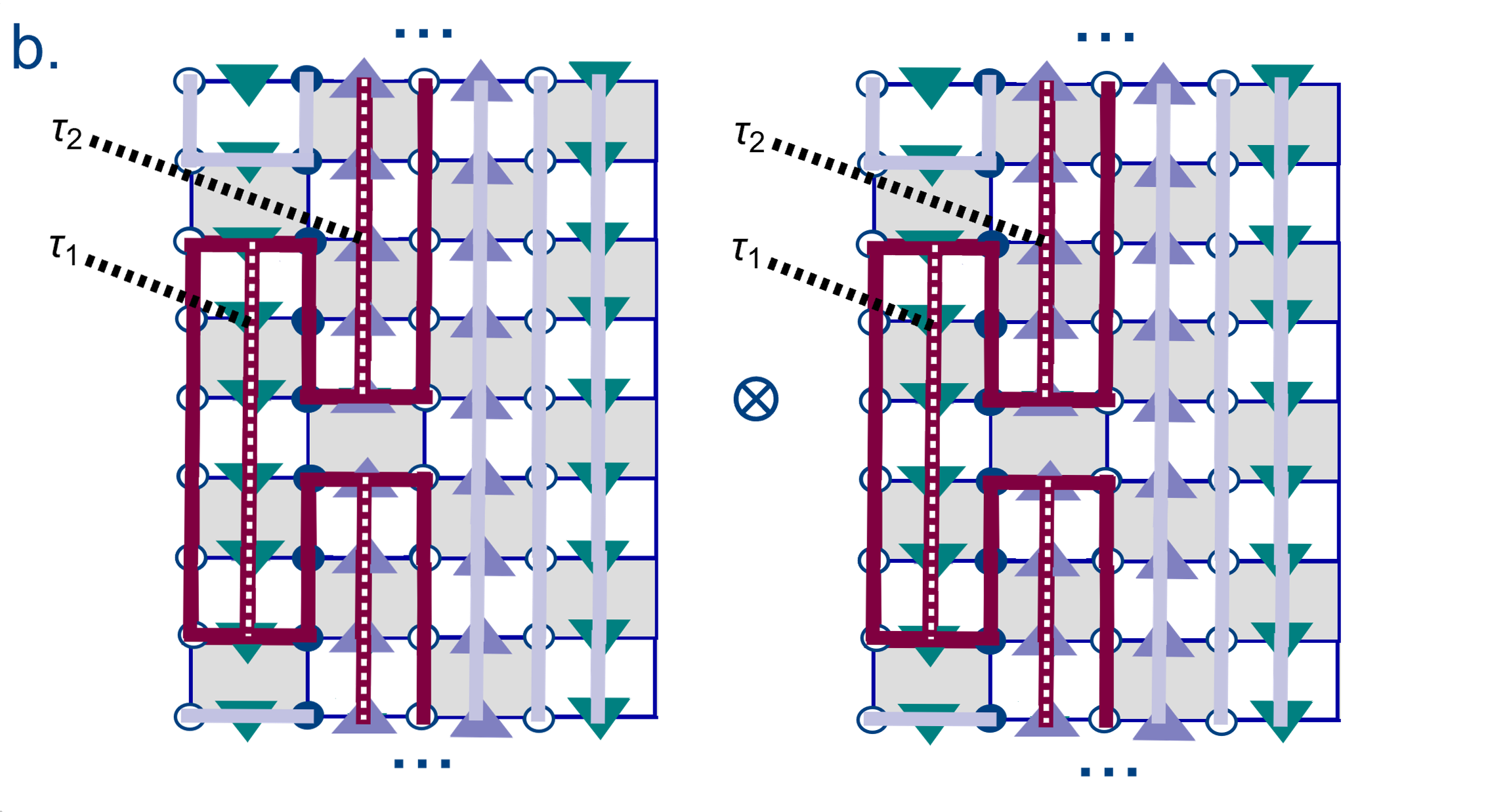
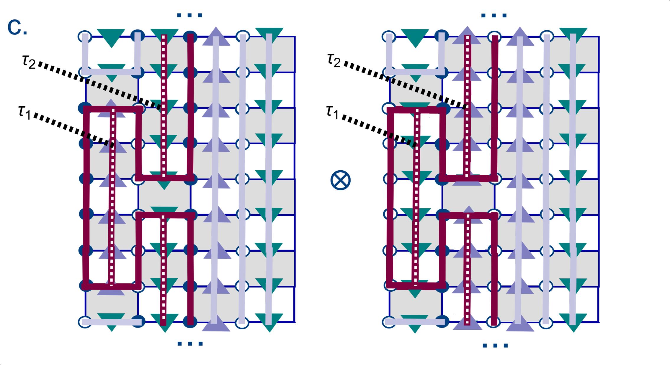
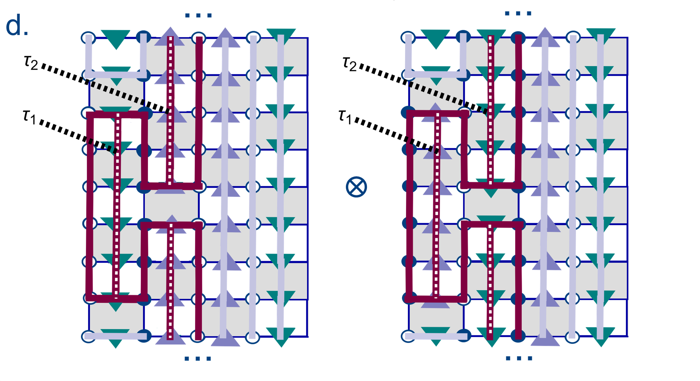
Figure 5: The spin factors of the weights for the portion of these terms that are shown (assuming the burgundy cluster is a meron) are: $e^{\tau_{1}J/4}e^{\tau_{2}J/4}$ for (a) and (b), and $e^{-\tau_{1}J/4}e^{-\tau_{2}J/4}$ for (c) and (d). Because the merons in (a) and (b) are positive and the merons in (c) and (d) are negative, the fully summed weight of the meron configuration will be positive. This assumes a staggered reference configuration where both layers are identical.

A.3 Additional Field Terms for the $U(1)$ Model

As discussed in the main text, the $U(1)$ model families have additional diagonal terms for the spins that may be added:

$$H^{U(1)}_{N_{f}=2}\rightarrow H^{U(1)}_{N_{f}=2}+J\sum_{\left\langle xy\right\rangle}s^{3}_{xy,1}s^{3}_{xy,2},$$ (17)

Here we discuss why these additions are sign-problem-free. Note that we will focus on the discrete-time version of the Meron Cluster algorithm, but the result also straightforwardly carries to continuous time. This addition is sign-problem-free for a similar reason that the addition of the Hubbard-$U$ term is sign-problem-free, as discussed in [48].

We apply the discrete time partition function expansion defined in the main text with general $d$ spatial dimensions, which is given for the new Hamiltonian $H^{\prime}$ by

$${\cal Z}={\mathrm{Tr}}\left(e^{-\beta H^{\prime}}\right)$$ (18)

$$\;=\sum_{\left\{s,n\right\}}\left\langle s_{1},n_{1}\right|e^{-\epsilon H_{a_{T}}^{\prime}}\left|s_{TN_{t}},n_{TN_{t}}\right\rangle$$

$$\qquad\left\langle s_{TN_{t}},n_{TN_{t}}\right|e^{-\epsilon H_{a_{T-1}}^{\prime}}\left|s_{TN_{t}-1},n_{TN_{t}-1}\right\rangle...$$

$$\qquad\left\langle s_{3},n_{3}\right|e^{-\epsilon H_{a_{2}}^{\prime}}\left|s_{2},n_{2}\right\rangle\left\langle s_{2},n_{2}\right|e^{-\epsilon H_{a_{1}}^{\prime}}\left|s_{1},n_{1}\right\rangle.$$

This Hamiltonian is Trotterized into $T$ sets of operators where the operators within each set commute with each other, $H^{\prime}=H_{a_{1}}^{\prime}+H_{a_{1}}^{\prime}+...+H_{a_{T}}^{\prime}$, thus there are $T\cdot N_{t}$ timeslices in this formula. In one spatial dimension, as seen in the main text, $T$ is $2$ and the Hamiltonian was divided into $H_{e}$ and $H_{o}$, for even and odd, respectively.

Writing in terms of the original $U(1)$ Hamiltonian $H$ (as simulated in this paper), we have

$${\cal Z}={\mathrm{Tr}}\left(e^{-\beta H}\right)$$ (19)

$$\;=\sum_{\left\{s,n\right\}}\left\langle s_{1},n_{1}\right|e^{-\epsilon\left(H_{a_{T}}+H^{s}_{a_{T}}\right)}\left|s_{TN_{t}},n_{TN_{t}}\right\rangle$$

$$\left\langle s_{TN_{t}},n_{TN_{t}}\right|e^{-\epsilon(H_{a_{T-1}}+H_{a_{T-1}}^{s})}\left|s_{TN_{t}-1},n_{TN_{t}-1}\right\rangle$$

$$\qquad\quad...\left\langle s_{3},n_{3}\right|e^{-\epsilon\left(H_{a_{2}}+H_{a_{2}}^{s}\right)}\left|s_{2},n_{2}\right\rangle$$

$$\quad\qquad\qquad\left\langle s_{2},n_{2}\right|e^{-\epsilon\left(H_{a_{1}}+H_{a_{1}}^{s}\right)}\left|s_{1},n_{1}\right\rangle,$$

where for example in $(1+1)$-$d$ we would have $a_{1}=o$, $a_{2}=e$, and

$$H_{e}^{s} =\sum_{x}s^{3}_{2x,2x+1,1}s^{3}_{2x,2x+1,2},$$ (20)

$$H_{o}^{s} =\sum_{x}s^{3}_{2x+1,2x+2,1}s^{3}_{2x+1,2x+2,2}.$$

Here we note that because these additional terms respect the gauge symmetry, we have for a generic Trotter operator set $a$,

$$e^{-\epsilon\left(H_{a}+H_{a}^{s}\right)}\left|s_{i}n_{i}\right\rangle =e^{-\epsilon H_{a}}e^{-\epsilon H_{a}^{s}}\left|s_{i}n_{i}\right\rangle$$ (21)

$$=e^{-\epsilon\left(h_{a}^{s}(s_{i})\right)}e^{-\epsilon H_{a}}\left|s_{i}n_{i}\right\rangle,$$

where $h_{a}^{s}(s_{i})$ is just a number that depends on the spin configuration at particular timeslice $i$, which is $s_{i}$.

Thus, we end up with a partition function very similar to our original one, but with the worldlines weighted slightly differently:

$${\cal Z}={\mathrm{Tr}}\left(e^{-\beta H}\right)$$ (22)

$$\;=\sum_{\left\{s,n\right\}}e^{-\epsilon\sum_{i}\left(h_{a_{1}}^{s}(s_{iT+1})+h_{a_{2}}^{s}(s_{iT+2})...h_{a_{T}}^{s}(s_{iT+T})\right)}$$

$$\left\langle s_{1},n_{1}\right|e^{-\epsilon H_{a_{T}}^{\prime}}\left|s_{TN_{t}},n_{TN_{t}}\right\rangle\left\langle s_{TN_{t}},n_{TN_{t}}\right|e^{-\epsilon H_{a_{T-1}}^{\prime}}$$

$$\qquad\qquad...e^{-\epsilon H_{a_{2}}^{\prime}}\left|s_{2},n_{2}\right\rangle\left\langle s_{2},n_{2}\right|e^{-\epsilon H_{a_{1}}^{\prime}}\left|s_{1},n_{1}\right\rangle.$$

Because of these additional weight factors, the merons no longer have zero weight, so the question is instead whether their weight can be guaranteed to be positive.

To figure out the meron weights, we consider a generic meron, a portion of which is illustrated in Fig. 5, noting that merons only appear in two spatial dimensions and higher, so the images in the figure would represent a cross-section of a $(2+1)$-$d$ (or higher dimensional) lattice, with two Trotter timeslices shown, and the others squashed since they are irrelevant to this portion of the meron. Here, we assume a staggered reference configuration of fermions that is identical for both spin layers. In the portion highlighted, the weight factors for the highlighted meron portions of the configurations (a) and (b) will have a positive sign because both layers have the same fermion configurations, and thus the sign contribution from each layer will be identical, leading to a positive product. The configurations (c) and (d) will have a negative sign factor coming from the highlighted meron because fermion occupations are flipped between the two layers. We have already established that the weights coming from the fermionic term are identical. The contributing factors for this meron portion that come from the spins are

$$e^{\tau_{1}J/4}e^{\tau_{2}J/4}$$ (23)

for configurations (a) and (b), and

$$e^{-\tau_{1}J/4}e^{-\tau_{2}J/4}$$ (24)

for configurations (c) and (d), because in the $U(1)$ theory spin degrees of freedom are tied to the fermion occupation numbers on either side of the $D$-breakups, and so if the fermions match in the two layers the spins must also match, and similarly if the fermions do not match in the two layers for the meron the spins also cannot match. Thus, the sum of the four configurations must be a positive number. We note that this also can be done for negative $J$-coupling, but there the staggered reference configuration changes to be opposite occupation numbers for the two layers.

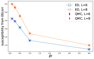
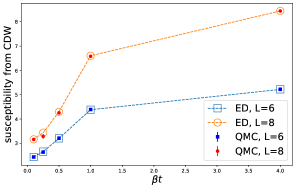
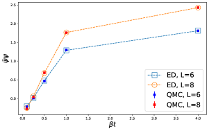
Figure 6: Comparison of Meron Cluster QMC values with the ED values for $\chi_{\mathrm{EEcorr}}$ (top), $\chi_{\mathrm{CDW}}$ (middle), and the bare $\bar{\psi}\psi$ (bottom).

$\mathbf{\beta t}$	$0.1$	$0.25$	$0.5$	$1.0$	$4.0$
$\chi_{\mathrm{EEcorr}}$, $L=6$
MC	2.60(3)	2.46(3)	2.08(2)	1.281(7)	0.7556(7)
ED	2.598	2.442	2.062	1.291	0.7542
$\chi_{\mathrm{EEcorr}}$, $L=8$
MC	3.49(4)	3.27(9)	2.76(6)	1.72(2)	0.9966(9)
ED	3.489	3.287	2.770	1.703	0.99606
$\chi_{\mathrm{CDW}}$, $L=6$
MC	2.44(4)	2.64(3)	3.21(3)	4.39(1)	5.2225(20)
ED	2.438	2.661	3.205	4.383	5.2197
$\chi_{\mathrm{CDW}}$, $L=8$
MC	3.16(4)	3.287(95)	4.26(8)	6.58(4)	8.443(4)
ED	3.164	3.440	4.299	6.603	8.445
$\bar{\psi}\psi$, $L=6$
MC	-0.22(2)	0.017(9)	0.47(1)	1.296(6)	1.8126(8)
ED	-0.210	0.0171	0.476	1.289	1.81284
$\bar{\psi}\psi$, $L=8$
MC	-0.28(2)	0.04(4)	0.68(3)	1.76(1)	2.432(1)
ED	-0.255	0.057	0.681	1.766	2.4322

Table 3: Results for the observables $\chi_{\mathrm{EEcorr}}$, $\chi_{CDW}$ and $\bar{\psi}\psi$ defined in (25) for the $U(1)$ model in $(1+1)$-$d$ calculated with Meron Clusters (MC) and exact diagonalization (ED).

A.4 Checks Against ED

For this paper we implemented the Meron Cluster method for the $U(1)$ theory in $1+1$-$d$, and for small lattices ($L=4$ and $L=8$) we have checked the following observables against exact diagonalization (ED) calculations:

$$\chi_{CDW} =\frac{1}{L_{t}}\sum_{x,y,t}(-1)^{x+y}\left(n_{x}-\frac{1}{2}\right)\left(n_{y}-\frac{1}{2}\right)$$ (25)

$$\bar{\psi}\psi =\frac{1}{L_{t}}\sum_{x,y,t}(-1)^{x}n_{x}$$

$$\chi_{\mathrm{EEcorr}} =\frac{1}{L_{t}}\sum_{x,y,t}s^{3}_{x,x+1}\cdot s^{3}_{y,y+1}.$$

Table 3 and Fig. 6 summarize these results, which are all for the observables in the Gauss law sector $G_{x}=0$.

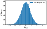
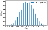
Figure 7: Probability density for the electric flux ${\cal E}$ for low temperature ($L=50$, $\beta t=8.0$) and high temperature ($L=22$, $\beta t=0.1$).

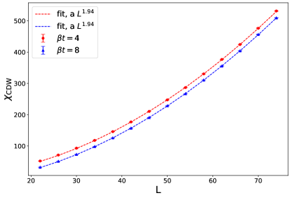
Figure 8: Divergence of the chiral condensate at low temperature.

A.5 Large volume physics with the Meron Algorithm

Although the fermion gauge coupling in the model we simulate with the meron algorithm is identical to the quantum link Schwinger model with spin-$\frac{1}{2}$, we have additional four fermion terms, which behave differently from the staggered mass term. While this interaction also induces an effective mass term, the mapping to a massive Schwinger model with renormalized parameters is non-trivial. This makes it hard to connect some of the large volume quantities to those usually studied in the literature [73, 74, 75, 76, 77, 78, 79]. Nevertheless, we present an empirical study of our measured observables.

In the main text we have shown the probability distribution of $\bar{\psi}\psi$ which shows a double peaked structure. We emphasize that each of the peaks correspond to one of the two Gauss’ Law sectors which emerge at low temperatures, indicating broken chiral symmetry. However, a corresponding histogram for the ${\cal E}$, the order parameter for the $CP$ symmetry (see Fig. 7 (left)) shows a symmetric distribution. This indicates constraining dynamics between the fermions and gauge fields: with the fermions constrained to occupy certain lattice sites at low temperatures, the gauge fields can fluctuate smoothly. This in turn means that the susceptibility corresponding to the electric flux (normalized to unit volume) cancel the cross terms (where $x\neq y$) and converges to the trivial value 0.125, contributed from the contact terms $(s_{x,x+1}^{3})^{2}$. We can characterize the fermionic order by measuring the divergence of the susceptibility of the charge density wave as a function of spatial volume, $L$. As we show in Fig. 8, the susceptibility diverges as $L^{1.94}$, for both $\beta t=4$ and $\beta t=8$. At high temperatures, on the other hand, the fermions can hop much more, which due to Gauss’ Law implies that the gauge fields are only allowed certain values. This is manifested in Fig. 7 (right) which shows the prominence of certain electric fluxes while others are highly suppressed. Moreover, this also explains the behaviour of the electric flux susceptibility in Fig. 4 of the main text: at low temperatures there is cancellation between the smooth electric fluxes, while at high temperatures the finite number of ${\cal E}$ values can multiply coherently to give rise to a large value of $\chi_{\cal E}$.

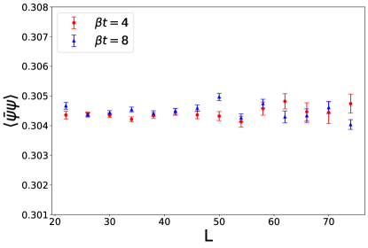
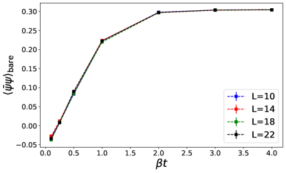
Figure 9: Bare chiral condensates for $U(1)$ theory in $1+1$-$d$ at low temperature and large lattices (top), while the temperature dependence of the condensate is bottom part of the figure.

It is also interesting to note that the presence of the large CDW order also indicates that the model develops a large chiral condensate $\bar{\psi}\psi$. For the model with staggered fermions, it is known that Gauss’ Law explicitly breaks the $\mathbb{Z}_{2}$ chiral symmetry of the model, which consists of a single spatial lattice translation [57]. The chiral condensate is thus large at small temperatures and as one increases the temperature, the condensate smoothly decreases and is expected to vanish at large temperatures. Since this is a crossover, there is no sharp behaviour in the condensate. Moreover, due to this explicit breaking of the $\mathbb{Z}_{2}$ symmetry by the Gauss Law, the chiral condensate undergoes additive renormalization in the Schwinger model. A similar phenomenology also happens in our model, but since we have a four-fermi coupling instead of a mass term, it is non-trivial to match the two models quantitatively without doing an extensive program involving non-perturbative renormalization. Nevertheless, on comparing the bare chiral condensate at low temperatures on large lattices in the thermodynamic limit, with the corresponding values quoted for the Schwinger model in Fig 15 of [76], we estimate that our model is equivalent to the Kogut-Susskind Schwinger model on the lattice with a bare mass of $am\sim 0.38-0.40$. In Fig. 9 (top), we show how the chiral condensate approaches a smooth thermodynamic limit. Moreover, in the bottom panel of Fig. 9, we also show the measurement of the chiral condensate with increasing temperatures until the condensate vanishes (and even becomes slightly negative at infinite temperatures), indicating a restoration of chiral symmetry at high temperatures. While it is qualitatively the same scenario in the Schwinger model [79], we refrain from getting into a technical discussion about the technical aspects of the renormalized chiral condensates in this paper.

References

- [1] Oskar Vafek and Ashvin Vishwanath. Dirac fermions in solids: From high-tc cuprates and graphene to topological insulators and weyl semimetals. Annual Review of Condensed Matter Physics, 5(1):83–112, 2014.
- [2] L. Borsten and M. J. Duff. Majorana fermions in particle physics, solid state and quantum information. pages 77–121, mar 2017.
- [3] Ian Johnston Rhind Aitchison and Anthony J G Hey. Gauge theories in particle physics: A practical introduction; 2nd ed. 1989.
- [4] Klaus von Klitzing. Quantum hall effect: Discovery and application. Annual Review of Condensed Matter Physics, 8(1):13–30, 2017.
- [5] José A. Flores-Livas, Lilia Boeri, Antonio Sanna, Gianni Profeta, Ryotaro Arita, and Mikhail Eremets. A perspective on conventional high-temperature superconductors at high pressure: Methods and materials. Physics Reports, 856:1–78, 2020. A perspective on conventional high-temperature superconductors at high pressure: Methods and materials.
- [6] Michael E. Peskin and Daniel V. Schroeder. An Introduction to quantum field theory. Addison-Wesley, Reading, USA, 1995.
- [7] Eduardo Fradkin. Field theoretic aspects of condensed matter physics: An overview, 2023.
- [8] Matthias Troyer and Uwe-Jens Wiese. Computational complexity and fundamental limitations to fermionic quantum Monte Carlo simulations. Phys. Rev. Lett., 94:170201, 2005.
- [9] Debasish Banerjee. Recent progress on cluster and meron algorithms for strongly correlated systems. Indian J. Phys., 95(8):1669–1680, 2021.
- [10] R. Blankenbecler, D. J. Scalapino, and R. L. Sugar. Monte carlo calculations of coupled boson-fermion systems. i. Phys. Rev. D, 24:2278–2286, Oct 1981.
- [11] F.F. Assaad and H.G. Evertz. World-line and Determinantal Quantum Monte Carlo Methods for Spins, Phonons and Electrons, pages 277–356. Springer Berlin Heidelberg, Berlin, Heidelberg, 2008.
- [12] F. F. Assaad, M. Bercx, F. Goth, A. Götz, J. S. Hofmann, E. Huffman, Z. Liu, F. Parisen Toldin, J. S. E. Portela, and J. Schwab. The ALF (Algorithms for Lattice Fermions) project release 2.0. Documentation for the auxiliary-field quantum Monte Carlo code. SciPost Phys. Codebases, page 1, 2022.
- [13] Shailesh Chandrasekharan. Fermion bag approach to lattice field theories. Phys. Rev. D, 82:025007, Jul 2010.
- [14] Congjun Wu and Shou-Cheng Zhang. Sufficient condition for absence of the sign problem in the fermionic quantum monte carlo algorithm. Phys. Rev. B, 71:155115, Apr 2005.
- [15] Emilie Fulton Huffman and Shailesh Chandrasekharan. Solution to sign problems in half-filled spin-polarized electronic systems. Physical Review B, 89(11), mar 2014.
- [16] Zi-Xiang Li, Yi-Fan Jiang, and Hong Yao. Solving the fermion sign problem in quantum monte carlo simulations by majorana representation. Phys. Rev. B, 91:241117, Jun 2015.
- [17] Lei Wang, Ye-Hua Liu, Mauro Iazzi, Matthias Troyer, and Gergely Harcos. Split orthogonal group: A guiding principle for sign-problem-free fermionic simulations. Phys. Rev. Lett., 115:250601, Dec 2015.
- [18] Zi-Xiang Li and Hong Yao. Sign-problem-free fermionic quantum monte carlo: Developments and applications. Annual Review of Condensed Matter Physics, 10(1):337–356, 2019.
- [19] Z. C. Wei, Congjun Wu, Yi Li, Shiwei Zhang, and T. Xiang. Majorana positivity and the fermion sign problem of quantum monte carlo simulations. Phys. Rev. Lett., 116:250601, Jun 2016.
- [20] Ori Grossman and Erez Berg. Unavoidable fermi liquid instabilities in sign problem-free models, 2023.
- [21] R. T. Scalettar, D. J. Scalapino, and R. L. Sugar. New algorithm for the numerical simulation of fermions. Phys. Rev. B, 34:7911–7917, Dec 1986.
- [22] J. E. Hirsch and R. M. Fye. Monte carlo method for magnetic impurities in metals. Phys. Rev. Lett., 56:2521–2524, Jun 1986.
- [23] Emanuel Gull, Andrew J. Millis, Alexander I. Lichtenstein, Alexey N. Rubtsov, Matthias Troyer, and Philipp Werner. Continuous-time monte carlo methods for quantum impurity models. Rev. Mod. Phys., 83:349–404, May 2011.
- [24] F. F. Assaad and T. C. Lang. Diagrammatic determinantal quantum monte carlo methods: Projective schemes and applications to the hubbard-holstein model. Phys. Rev. B, 76:035116, Jul 2007.
- [25] Lei Wang, Ye-Hua Liu, and Matthias Troyer. Stochastic series expansion simulation of the model. Phys. Rev. B, 93:155117, Apr 2016.
- [26] Emilie Huffman and Shailesh Chandrasekharan. Fermion bag approach to hamiltonian lattice field theories in continuous time. Phys. Rev. D, 96:114502, Dec 2017.
- [27] Ulli Wolff. Collective monte carlo updating for spin systems. Phys. Rev. Lett., 62:361–364, Jan 1989.
- [28] Hans Gerd Evertz, Gideon Lana, and Mihai Marcu. Cluster algorithm for vertex models. Phys. Rev. Lett., 70:875–879, Feb 1993.
- [29] B. B. Beard and U.-J. Wiese. Simulations of discrete quantum systems in continuous euclidean time. Phys. Rev. Lett., 77:5130–5133, Dec 1996.
- [30] Ribhu K Kaul and Matthew S Block. Numerical studies of various néel-VBS transitions in SU() anti-ferromagnets. Journal of Physics: Conference Series, 640:012041, sep 2015.
- [31] Anders W. Sandvik. Stochastic series expansion methods, 2019.
- [32] Anders W. Sandvik and Bowen Zhao. Consistent scaling exponents at the deconfined quantum-critical point. Chin. Phys. Lett., 37(5):057502, 2020.
- [33] S. Duane, A. D. Kennedy, B. J. Pendleton, and D. Roweth. Hybrid Monte Carlo. Phys. Lett. B, 195:216–222, 1987.
- [34] I. Montvay and G. Munster. Quantum fields on a lattice. Cambridge Monographs on Mathematical Physics. Cambridge University Press, 3 1997.
- [35] Thomas DeGrand and Carleton E. Detar. Lattice methods for quantum chromodynamics. World Scientific, 2006.
- [36] Stefan Beyl, Florian Goth, and Fakher F. Assaad. Revisiting the Hybrid Quantum Monte Carlo Method for Hubbard and Electron-Phonon Models. Phys. Rev. B, 97(8):085144, 2018.
- [37] P. V. Buividovich and M. V. Ulybyshev. Applications of lattice QCD techniques for condensed matter systems. International Journal of Modern Physics A, 31(22):1643008, aug 2016.
- [38] Maksim Ulybyshev, Savvas Zafeiropoulos, Christopher Winterowd, and Fakher Assaad. Bridging the gap between numerics and experiment in free standing graphene, 2021.
- [39] Peter Lunts, Michael S. Albergo, and Michael Lindsey. Non-hertz-millis scaling of the antiferromagnetic quantum critical metal via scalable hybrid monte carlo, 2022.
- [40] Beat Ammon, Hans Gerd Evertz, Naoki Kawashima, Matthias Troyer, and Beat Frischmuth. Quantum monte carlo loop algorithm for the model. Phys. Rev. B, 58:4304–4319, Aug 1998.
- [41] M. Brunner and A. Muramatsu. Quantum monte carlo simulations of infinitely strongly correlated fermions. Phys. Rev. B, 58:R10100–R10103, Oct 1998.
- [42] N. Kawashima, J. E. Gubernatis, and H. G. Evertz. Loop algorithms for quantum simulations of fermion models on lattices. Phys. Rev. B, 50:136–149, Jul 1994.
- [43] Christof Gattringer. Density of states techniques for fermion worldlines, 2022.
- [44] W. Bietenholz, A. Pochinsky, and U. J. Wiese. Meron-cluster simulation of the vacuum in the 2d o(3) model. Physical Review Letters, 75(24):4524–4527, dec 1995.
- [45] Shailesh Chandrasekharan and Uwe-Jens Wiese. Meron cluster solution of a fermion sign problem. Phys. Rev. Lett., 83:3116–3119, 1999.
- [46] S. Chandrasekharan, J. Cox, J. C. Osborn, and U. J. Wiese. Meron cluster approach to systems of strongly correlated electrons. Nucl. Phys. B, 673:405–436, 2003.
- [47] F. F. Assaad and Tarun Grover. Simple Fermionic Model of Deconfined Phases and Phase Transitions. Phys. Rev. X, 6(4):041049, 2016.
- [48] Hanqing Liu, Shailesh Chandrasekharan, and Ribhu K. Kaul. Hamiltonian models of lattice fermions solvable by the meron-cluster algorithm. Phys. Rev. D, 103(5):054033, 2021.
- [49] E. A. Martinez et al. Real-time dynamics of lattice gauge theories with a few-qubit quantum computer. Nature, 534:516–519, 2016.
- [50] Hannes Bernien, Sylvain Schwartz, Alexander Keesling, Harry Levine, Ahmed Omran, Hannes Pichler, Soonwon Choi, Alexander S. Zibrov, Manuel Endres, Markus Greiner, and et al. Probing many-body dynamics on a 51-atom quantum simulator. Nature, 551(7682):579–584, Nov 2017.
- [51] N. Klco, E. F. Dumitrescu, A. J. McCaskey, T. D. Morris, R. C. Pooser, M. Sanz, E. Solano, P. Lougovski, and M. J. Savage. Quantum-classical computation of schwinger model dynamics using quantum computers. Physical Review A, 98(3), Sep 2018.
- [52] Zohreh Davoudi, Indrakshi Raychowdhury, and Andrew Shaw. Search for Efficient Formulations for Hamiltonian Simulation of non-Abelian Lattice Gauge Theories. 9 2020.
- [53] D. Banerjee, S. Caspar, F. J. Jiang, J. H. Peng, and U. J. Wiese. Nematic confined phases in the quantum link model on a triangular lattice: An opportunity for near-term quantum computations of string dynamics on a chip. 2021.
- [54] Emilie Huffman, Miguel García Vera, and Debasish Banerjee. Toward the real-time evolution of gauge-invariant and quantum link models on noisy intermediate-scale quantum hardware with error mitigation. Phys. Rev. D, 106(9):094502, 2022.
- [55] Sepehr Ebadi et al. Quantum phases of matter on a 256-atom programmable quantum simulator. Nature, 595(7866):227–232, 2021.
- [56] S. Chandrasekharan and U. J. Wiese. Quantum link models: A Discrete approach to gauge theories. Nucl. Phys., B492:455–474, 1997.
- [57] D. Banerjee, M. Dalmonte, M. Muller, E. Rico, P. Stebler, U. J. Wiese, and P. Zoller. Atomic Quantum Simulation of Dynamical Gauge Fields coupled to Fermionic Matter: From String Breaking to Evolution after a Quench. Phys. Rev. Lett., 109:175302, 2012.
- [58] Shailesh Chandrasekharan. Solutions to sign problems in lattice Yukawa models. Phys. Rev. D, 86:021701, 2012.
- [59] Emilie Huffman and Shailesh Chandrasekharan. Solution to sign problems in models of interacting fermions and quantum spins. Phys. Rev. E, 94:043311, Oct 2016.
- [60] Ribhu K. Kaul, Roger G. Melko, and Anders W. Sandvik. Bridging lattice-scale physics and continuum field theory with quantum monte carlo simulations. Annual Review of Condensed Matter Physics, 4(1):179–215, apr 2013.
- [61] Uwe-Jens Wiese. From quantum link models to D-theory: a resource efficient framework for the quantum simulation and computation of gauge theories. Phil. Trans. A. Math. Phys. Eng. Sci., 380(2216):20210068, 2021.
- [62] Snir Gazit, Mohit Randeria, and Ashvin Vishwanath. Emergent dirac fermions and broken symmetries in confined and deconfined phases of z2 gauge theories. Nature Physics, 13(5):484–490, feb 2017.
- [63] Snir Gazit, Fakher F. Assaad, Subir Sachdev, Ashvin Vishwanath, and Chong Wang. Confinement transition of gauge theories coupled to massless fermions: Emergent quantum chromodynamics and symmetry. Proceedings of the National Academy of Sciences, 115(30), jul 2018.
- [64] Xiao Yan Xu, Yang Qi, Long Zhang, Fakher F. Assaad, Cenke Xu, and Zi Yang Meng. Monte carlo study of lattice compact quantum electrodynamics with fermionic matter: The parent state of quantum phases. Phys. Rev. X, 9:021022, May 2019.
- [65] Umberto Borla, Ruben Verresen, Fabian Grusdt, and Sergej Moroz. Confined phases of one-dimensional spinless fermions coupled to gauge theory. Physical Review Letters, 124(12), mar 2020.
- [66] Jernej Frank, Emilie Huffman, and Shailesh Chandrasekharan. Emergence of gauss' law in a z2 lattice gauge theory in dimensions. Physics Letters B, 806:135484, jul 2020.
- [67] Tomohiro Hashizume, Jad C. Halimeh, Philipp Hauke, and Debasish Banerjee. Ground-state phase diagram of quantum link electrodynamics in -d. SciPost Phys., 13(2):017, 2022.
- [68] R. M. Fye. New results on trotter-like approximations. Phys. Rev. B, 33:6271–6280, May 1986.
- [69] Shailesh Chandrasekharan and James Osborn. Solving Sign Problems with Meron Algorithms. Springer Proc. Phys., 86:28–42, 2000.
- [70] Yi-Ping Huang, Debasish Banerjee, and Markus Heyl. Dynamical quantum phase transitions in u(1) quantum link models. Phys. Rev. Lett., 122:250401, Jun 2019.
- [71] Paul Fendley, K. Sengupta, and Subir Sachdev. Competing density-wave orders in a one-dimensional hard-boson model. Phys. Rev. B, 69:075106, Feb 2004.
- [72] Federica M. Surace, Paolo P. Mazza, Giuliano Giudici, Alessio Lerose, Andrea Gambassi, and Marcello Dalmonte. Lattice gauge theories and string dynamics in rydberg atom quantum simulators. Phys. Rev. X, 10:021041, May 2020.
- [73] Sidney R. Coleman, R. Jackiw, and Leonard Susskind. Charge Shielding and Quark Confinement in the Massive Schwinger Model. Annals Phys., 93:267, 1975.
- [74] Sidney R. Coleman. More About the Massive Schwinger Model. Annals Phys., 101:239, 1976.
- [75] Kirill Melnikov and Marvin Weinstein. The Lattice Schwinger model: Confinement, anomalies, chiral fermions and all that. Phys. Rev. D, 62:094504, 2000.
- [76] T. Byrnes, P. Sriganesh, R. J. Bursill, and C. J. Hamer. Density matrix renormalization group approach to the massive Schwinger model. Phys. Rev. D, 66:013002, 2002.
- [77] Boye Buyens, Frank Verstraete, and Karel Van Acoleyen. Hamiltonian simulation of the Schwinger model at finite temperature. Phys. Rev. D, 94(8):085018, 2016.
- [78] M. C. Bañuls, K. Cichy, J. I. Cirac, K. Jansen, and H. Saito. Thermal evolution of the Schwinger model with Matrix Product Operators. Phys. Rev. D, 92(3):034519, 2015.
- [79] Mari Carmen Bañuls, Krzysztof Cichy, Karl Jansen, and Hana Saito. Chiral condensate in the Schwinger model with Matrix Product Operators. Phys. Rev. D, 93(9):094512, 2016.
- [80] Torsten V. Zache, Maarten Van Damme, Jad C. Halimeh, Philipp Hauke, and Debasish Banerjee. Toward the continuum limit of a ð1 + 1ÞD quantum link Schwinger model. Phys. Rev. D, 106(9):L091502, 2022.