Fast Estimation of Physical Error Contributions of Quantum Gates

Abstract

Large-scale quantum computation requires a fast assessment of the main sources of error in the implemented quantum gates. To this aim, we provide a learning based framework that allows to extract the contribution of each physical noise source to the infidelity of a series of gates with a small number of experimental measurements. To illustrate this method, we consider the case of superconducting transmon architectures, where we focus on the diabatic implementation of the CZ gate with tunable couplers. In this context, we account for all relevant noise sources, including non-Markovian noise, electronics imperfections and the effect of tunable couplers to the error of the computation.

I Introduction

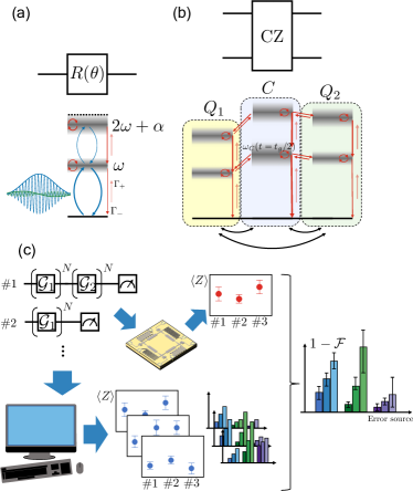
Figure 1: (a) A standard implementation of single-qubit rotations around the $x$ or $y$ axes, based on applying two separate out of phase microwave pulses, which can also excite the population outside of the computational subspace in weakly non-linear ($|\alpha|\ll\omega$) superconducting qubits. Additionally, incoherent decay from the excited states and pure dephasing are represented with red arrows. The uncertainty of the energy levels represents the effect of $1/f$-type flux noise and long timescale drifts. (b) The energy level diagram of a tunable coupler based CZ gate implementation. Because of the near resonance between the coupler and qubit excited states a global (i.e. non-local) Lindblad equation is needed to describe the incoherent dynamics (red arrows). All three parts of the system are coupled, as denoted by the double sided arrows beneath. (c) Scheme to extract information of the infidelity contribution from different error sources. Supervised learning techniques are used to interpolate between simulation results for different parameters and an experimental result. The setup requires considering the same gate $N$ times so that errors are sufficiently amplified to facilitate the discernment of its different contributions. Taking into account state preparation and measurement errors, we are then able to estimate the magnitude of each error source and the corresponding uncertainties.

In recent years, there has been a steady advance in the scale and quality of quantum computing architectures, although the presence of noise and imperfections in the system remains a vital issue holding back the achievement of quantum advantage. An accurate diagnosis of the physical origin of the errors is key to specifically tailor hardware modifications, fabrication or calibration procedures to tackle the problem. In addition, noise-aware error mitigation techniques [1] require a detailed understanding of the noise processes in the system, while error correcting codes, which currently assume the hardware noise to be completely uncorrelated, will require tackling more complex error sources such as leakage [2] to advance beyond state of the art experiments [3, 4].

The noise present in quantum circuits is typically modelled by appending specific noise channels after the application of each gate in the algorithm [5, 6, 7]. These noise channels can be reconstructed experimentally, or constructed based on a predefined model together with some experimentally measured parameters. However, this approach contains a number of implicit assumptions about the underlying error processes, namely that the noise contains no temporal or spatial correlation, is trace-preserving and small in the operator norm sense.

While the above modelling is a good first approach to predict the approximate performance of an algorithm, many of its assumptions are not justified in a realistic circuit execution. Considering superconducting qubits as an example, many experiments report a longer spin echo dephasing time compared to a Ramsey decay time [8, 9, 3, 10], directly demonstrating the presence of time-correlated or non-Markovian noise. Moreover, the second-excited level of a transmon plays a major role in the implementation of single-qubit rotations, and is currently one of the major infidelity contributors to such operations, even though such a noise channel is not trace preserving in the truncated qubitized subspace [11]. Furthermore, many two-qubit gate implementations rely on the transfer of the population outside of the computational subspace, meaning that an imperfect calibration will often result in a part of the population remaining outside of of the computational subspace. Since many state-of-the art quantum computing architectures employ non-computational elements on the chip, such as tunable couplers, the effect of leakage into tunable coupler states is even more convoluted [9, 12, 13, 14, 10, 15, 16, 17].

This evidence has driven the community to develop benchmarking and characterization methods beyond the standard assumptions. While typical noise characterization protocols such as, e.g., Gate Set Tomography (GST) [18] or Randomized Benchmarking (RB) [19], still operate under the same assumptions, some of them have recently been extended to also include non-Markovian effects [20, 21, 22], including upgraded functionalities to differentiate different kinds of non-Markovianity [23]. Other proposals have focused on the use of phenomenological non-Markovian master equations to describe and predict the dynamics of superconducting quantum computing processors [24, 25, 26].

The above are very important advances in our understanding of the presence and impact of complex errors in the system, but assessing their physical origin is key to developing accurate error suppression, mitigation and correction techniques. In this regard, GST has been extended to connect the reconstructed errors to specific physical noise sources within the Markovian approximation [27, 28]. However, an accurate characterization of the main error sources, including more complex ones such as correlated noise and leakage errors, presents a mayor drawback: accessing every single error parameter necessitates dedicated experiments or may even be untractable in some cases. Moreover, even if a gate is well-characterized at one point in time, due to the drifts that may occur in both the qubits and their environment, the error contributions will evolve over time [29]. These temporal drifts mean that the operations we implement must be re-calibrated on a regular basis. In the very near future, when chips are scaled to large numbers, we therefore need a fast procedure to characterize the errors in the quantum computers, in order to minimize the time needed for the re-calibration.

In this paper we present a new error budgeting approach that enables efficiently accessing the contribution of the main noise sources to the system infidelity. The method is based on comparing experimental measurements with precomputed simulations obtained for a broad range of parameters, in order to avoid having to chararacterize all of the noise parameters individually. Thus, our method substantially differs from previous ones based on an adaptive approach, where the computational and experimental efforts are concentrated on finding the simulation with a complete set of noise parameters that best describes the system dynamics. Interestingly, this new diagnosis scheme allows to gain knowledge about errors that are hard to parameterize with more general benchmarking techniques, such as those that are non-Markovian or non-trace-preserving, and is general to any quantum computing platform where the dynamics can be modelled sufficiently accurately. This technique is sketched in Fig. 1(c).

We illustrate this method by considering transmon-based superconducting qubit devices. To this aim, we have developed what perhaps is the most complete error modelling framework existing for such devices. The proposed framework remains simple enough to be efficiently simulated, as required by our budgeting scheme. Finally, we discuss the results obtained for the contribution of the different error sources to the infidelity of different gate sequences.

The paper is organized as follows: We first describe the relevant physical error sources of both single and two-qubit quantum gates in Sec. III. In Section IV we show how such physical noise processes can be efficiently simulated, even when including non-Markovian dynamics, before demonstrating their effects on the gate performance in Sec. V.3. In Sec. V.4 we describe our learning-based, approach to diagnose gate errors.

II Reconstructing Error Budgets Based on Noise Modelling

In this section we describe our proposed scheme to extract information about the infidelity contribution from realistic devices. The scheme uses supervised learning techniques to interpolate between simulations, obtained with different noise parameter values, and an experimental result. This allows us to make comparisons between experiments and the most similar simulations and extract the infidelity contributions. We use Gaussian Process Regression (GPR), a widely successful machine learning technique with demonstrated uses in different fields ranging from geostatistics [30], material science [31] and also the modelling of classical integrated circuits [32, 33]. The main benefits of using GPR are the inherent uncertainty predictions based on the similarity of the experimental values to the simulated ones, the representational flexibility, as well as typically smaller training samples [34].

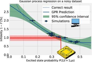
Figure 2: An illustrative scheme of a simplified scheme to measure the $T_{1}$ decay induced infidelity using a single input experiment and GPR. The input experiment used in this case consists of preparing a qubit in the excited state and waiting for 1 $\mu s$ before measuring the excited state ($x$-axis). The data points correspond to a number of simulated qubit evolutions with different $T_{1}$ decay times, and different measurement errors indicated by the horizontal error bars. An interpolation of these points using GPR is plotted with the solid blue line, with the shaded area representing the uncertainty of the GPR prediction due to state preparation or measurement errors. As a reference, the exact relationship between the measured excited state probability and a single-qubit gate infidelity ($y$-axis) is plotted with the dotted blue line. In general, this relationship is typically not known, due to the presence of different error sources, and numerical simulations are the only available probe. According to the proposed method, when an experimental result is obtained (vertical red solid line), the GPR prediction curve would allow to determine the corresponding infidelity (horizontal red solid line). Furthermore, an estimate of the accuracy of this prediction due to the GPR prediction is depicted with the shaded red area. The correct value is plotted with the horizontal dotted red line.

While standard characterization is based on performing a number of different experiments to obtain the parameters of each noise model, our proposal is experimentally less costly, as it outputs the desired error budget by comparing a smaller number of experiments with low shot numbers to a large number of simulation results. Unlike typical gate calibration procedures [9], we also assume that we only have access to circuit level results.

To be more specific, currently, if one wishes to extract the information about the error budgets of the quantum gates, the general workflow of such a procedure is described by the following steps:

1. Construct a model of the noise in the system.

2. Perform a number of experiments needed to characterize the noise model.

3. Extract model parameters from experimental measurements.

4. Simulate the model with the measured parameters and extract the relevant information about the error budget.

5. Validate model on new experiments.

However, extracting all the relevant parameters of the noise is costly, or even not-doable, like in the presence of non-Markovian effects, generally produced by complex environments that need to be fully characterized, or when having to infer the properties of the non-computational and non-accessible elements such as couplers in the case of superconducting qubits. We therefore propose an alternative approach of extracting similar information, which has been sketched in Fig. 1(c):

1. Construct a physical noise model of the system.

2. Simulate different experiments with a large number of different parameters.

3. Perform the experiments on real hardware.

4. Systematically compare the similarity between the different simulations and experiment.

What is crucial is the last point in the list. If the experimental measurements coincide with a simulation for a specific set of noise parameters, we can be fairly certain that our model is sufficiently accurate and the noise parameters in experiment are the ones we used for the simulation, however this is rarely the case. Even if our model was perfect we will likely never perfectly guess the correct parameters and this must be reflected in the certainty of our predictions. We therefore need to base the error bars of our reconstructed error budgets on the difference between the experimental measurement and the most similar simulations.

The predictions from the experimental input are then given by interpolating the values from the simulation, while the uncertainties of the predictions are given by two sources. The first is the similarity of the simulated and experimental inputs, and the second is the inherent uncertainty of the measured results, either due to finite sampling noise or state preparation and measurement errors. More formally, we do this by using Gaussian Process Regression (GPR)[34].

In other words, we use the trained GPR as a model to describe the more complex relationship between the outcomes of circuit executions and the infidelity contributions, similarly to the scheme proposed in Ref. [35]. A naive simplified example of how this procedure can be employed is illustrated in Fig. 2. The example in Fig. 2 only covers one error source and one input experiment, but realistically more experiments can be used as an input, and each error source warrants its own GPR model (since the error sources are independent of each other). We stress again, that in a practical setting, due to the presence of several error sources, it is difficult to disentangle the individual contributions from circuit execution data.

GPR is a Bayesian regression method based on finding the optimal Gaussian process which best fits the data. A Gaussian process is a stochastic process characterized by a multivariate Gaussian probability distribution. More details about the implementation of GPR can be found in Appendix A. The main benefits of using Gaussian processes to interpolate the data is their ability to predict the uncertainty of the outputs, which is not the case for most other regression or machine learning models. Additionally, this method does not require unrealistically large amounts of data, with training sets on the order of 500 simulations being typically enough, however this depends on the uncertainty of the parameters we are considering.

It can be shown that GPR is a universal function approximator, meaning that it can be used to model complex non-linear relationships [36], however it is also important to note that since the optimization of the GPR parameters can be costly and non-convex, we typically repeat the training step several times in order to obtain the most optimal solution [34]. The complexity of the model can be easily increased or decreased by modifying the kernel function (see Appendix A) and it is typically evident from the optimized parameters when the model complexity is sufficient.

The uncertainty of the predictions of a properly optimized GPR model are typically low in the vicinity of the training inputs, and larger further away. Practically, this means that if the experimental input is significantly different from the simulated sample, the GPR model will return large uncertainties, giving us a clear signal that our theoretical model predictions, within the parameter ranges we have simulated, do not adequately explain the experiment, which is crucial knowledge since no model will ever be perfect. Another source of uncertainty in the predictions is the inherent noisiness of the input output pairs, since we are, e.g., fundamentally limited in precision by the finite number of shots used to probe the system.

We can see that in both the standard and our alternative approach, one has to specify a noise model at one point or another, so we are not restricting ourselves significantly more than in the standard approach. If we are not able to model the noise accurately, then there is no way to estimate the effect of a noise source on the gate with any type of procedure.

One drawback of the alternative approach compared to the standard methods is therefore not the physical modelling of the noise in the gates we are interested in, but state preparation and measurement (SPAM) errors, which therefore must be taken into account in the simulation sample. We have described how we simulate these in Secs. IV.1, IV.3. If this modelling of the SPAM errors is not correct, we will see this as model violation, i.e. large uncertainties in the predictions.

Alternatively, one could define a similar characterization scheme without having a large precomputed sample of simulations, based on an optimization loop which finds the best model parameters. However, noisy simulations of quantum systems, especially with non-Markovian effects, tend to be very demanding so by precomputing a larger sample, we can efficiently parallelize our simulations, thus drastically reducing the computational time needed.

III Physical Error Sources of Quantum Gates

In this section we will present all the error sources currently limiting the gate fidelities of transmon quantum computers. Here we will also make the distinction between an error source and an error type. As an example, consider leakage to the higher levels of a transmon during a single-qubit gate operation - we consider this to be an error type, which can have several error sources, such as e.g. non-unitary heating transitions or unitary leakage dynamics due to the small anharmonicity. In detail,

• We improve the modelling of environmental effects in the two-qubit gate scheme. Namely the $T_{1}$ decay by considering the many-body effects in the non-unitary dynamics derived from the Hamiltonian of a physically realistic environment of two-level systems (TLSs), as well as considering the non-Markovian flux noise as a more realistic description of the pure dephasing of flux-tunable transmons. The main error contributions for single and two-qubit gates are sketched in Figs. 1(a) and 1(b), respectively. A similarly detailed Hamiltonian modelling of noise in ion trap systems, with good experimental agreement can be found in Ref. [37] .

• Additionally we have compiled realistic estimates on the accuracy of the control electronics and calibration procedure. We have focused on the most common microwave pulse driven single-qubit gates with the DRAG pulse scheme [11] and the non-adiabatic implementation of the controlled-Z (CZ) gate in a tunable coupler architecture [9, 12, 13, 4]. For two-qubit gates we have chosen an implementation that has shown very high fidelities, does not suffer from residual ZZ interaction and has been implemented as the native entangling operation in some of the most significant experiments in field [38, 4, 39] by companies such as Google, with also IBM having recently announced a tunable coupler based chip [40, 17]. Additionally, it has been shown that the tunable coupler based CZ gate can also be extended to co-design processors, such as the one presented in Ref. [41].

While the models presented in this section could always be further improved, they capture the most relevant dynamics, while still being tractable in simulation.

III.1 Single-Qubit Gates

We model the transmon as a driven anharmonic oscillator, with a Hamiltonian of the form

$$\hat{H}=\omega\,\hat{a}^{\dagger}\hat{a}+\frac{\alpha}{2}\hat{a}^{\dagger}\hat{a}^{\dagger}\hat{a}\hat{a}-i\Omega(t)\left(\hat{a}-\hat{a}^{\dagger}\right),$$ (1)

where $\hat{a}$ are bosonic annihilation operators, $\omega$ is the frequency of the qubit and $\alpha$ is the anharmonicity. The last term above represents the action of the control waveform parametrized by the function $\Omega(t)$, which is additionally parameterized by the two quadrature controls $I(t)$ and $Q(t)$ so that

$$\Omega(t)=I(t)\sin\left(\omega_{d}t\right)+Q(t)\cos\left(\omega_{d}t\right).$$ (2)

We accentuate here that the frequency of the drive $\omega_{d}$ and the transmon transition frequency $\omega$ are not necessarily equal [42].

The above parametrization is useful when employing the pulse shape known as Derivative Removal by Adiabatic Gate (DRAG) [11]. This pulse shape is commonly used due to its effectiveness in reducing leakage to the $f$-state of the transmon, as well as its simplicity and therefore ease of calibration. The DRAG scheme is very straightforward, and consists of applying any finite pulse shape $s_{0}(t)$ on one quadrature, and its scaled derivative $s_{1}(t)\propto\dot{s}_{0}(t)$ on the other [11]. More specifically, we use Gaussian pulses defined by

$$s_{0}(t) =\begin{cases}A\exp\left(-\frac{(t-\mu)^{2}}{2\sigma^{2}}\right)-B&\text{if }0<t<T,\\ 0&\text{else. }\end{cases}$$ (3)

$$s_{1}(t) =-\beta\frac{t-\mu}{\sigma^{2}}s_{0}(t).$$ (4)

In other words, $s_{0}(t)$ is a Gaussian envelope with a finite time cut-off $T$, and $s_{1}(t)$ is the re-scaled derivative of $s_{0}(t)$. By using $I(t)=s_{0}(t)$ and $Q(t)=s_{1}(t)$, or $I(t)=s_{1}(t)$ and $Q(t)=s_{0}(t)$, we can choose between implementing qubit rotations around the $X$ or $Y$-axes of the Bloch sphere.

The parameters $\sigma$, $\mu$ and $T$ are considered to be fixed, while $A$ and $\beta$ are tuned in the calibration procedure. The offset $B$ is set so that the truncated Gaussian curve does not have any discontinuities, i.e. $s_{0}(t=0)=s(t=T)=0$. This definition assumes the pulse is performed at time $t=0$, however if this is not the case, as we are also interested in performing simulations of multiple gates, the formulas are translated so that $s_{0,\tau(t)}=s_{0}(t-\tau)$ so that the pulse begins at time $\tau$.

All of our single-qubit gate simulations also include some electronics imperfections such as the finite sampling rate, which we fix to $1/\delta t=2.4$ GHz. This means the real output of the electronics is given by discretized values

$$\tilde{I}(t)=I\left(\left\lfloor\frac{t}{\delta t}\right\rfloor\delta t\right),$$ (5)

and equivalently for the second quadrature $Q(t)$. While we always assume our pulse is continuous when programming the pulse shapes, the output is actually to be discretized.

III.1.1 Amplitude damping errors

One of the best-known error sources is amplitude damping characterized by the so-called $T_{1}$ decay time, which can be easily measured by preparing the qubit in the excited state and measuring the population at different times.

It is believed that for current hardware the observed $T_{1}$ times are limited by the coupling of the transmon to a bath of two-level systems (TLSs) [43, 44, 45, 46]. The interaction originates from the coupling of the TLS electric dipole to the transmons charge degree of freedom [47]. There are also other physical contributions to $T_{1}$ such as e.g. interactions with non-equilibrium Bogoliubov quasi-particles, however their effect was found to be smaller in some studies on transmon qubits [48, 49], in the absence of burst events [50].

Except for rare occasions of resonant qubit-TLS interactions, the observed $T_{1}$ decays are well-described by an exponential curve [29], and therefore modelled with the Markovian approximation. Motivated by the results of Ref. [51], where the qubit effective temperature was shown to be considerably higher than the cryostat temperature and can result in excited state populations in the order of 1% [52, 53, 54], we also consider that the bath producing the $T_{1}$ decay is at a finite temperature, which means that there is a finite heating rate in the model.

We use the Lindblad equation to simulate the dynamics of such finite temperature $T_{1}$ decay

$$\frac{\mathrm{d}\hat{\rho}}{\mathrm{d}t}=-i\left[\hat{H},\hat{\rho}\right]+\sum_{i=+,-}\Gamma^{i}_{1}\left(\hat{C}_{i}\hat{\rho}\hat{C}_{i}^{\dagger}+\frac{1}{2}\left\{\hat{C}_{i}^{\dagger}\hat{C}_{i},\hat{\rho}\right\}\right),$$ (6)

with $\hat{C}_{-}=\hat{a}$ and $\hat{C}_{+}=\hat{a}^{\dagger}$ and the $T_{1}$ decay rate in a standard excited state population decay experiment is given by $\Gamma_{1}=\Gamma^{+}_{1}+\Gamma^{-}_{1}$. The ratio of both rates is determined by the detailed balance condition $\Gamma_{1}^{+}/\Gamma_{1}^{-}=e^{-\omega/k_{B}T_{\mathrm{eff}}}$, which is valid if we assume the qubit is embedded in a thermalized environment [55]. The exponential suppression of the heating rate $\Gamma_{1}^{+}$ implies that it has a small effect on the dynamics itself. Nevertheless, it has a significant effect on the state preparation, as it means that the qubit has some residual excited state population initially.

In this model, the decay rate from the second to first excited state is exactly twice the rate of the excited to ground state transition, which is in reasonable agreement with the transmon qutrit decay rates reported in Refs. [56, 57].

Finally, the above equation is completely independent of the origin of the decay process, as all the characteristics of the environment are reduced to two rates.

III.1.2 Markovian Pure Dephasing

In the majority of cases, it is observed that the $T_{2}$ decay time measured in a Ramsey experiment, of a qubit is not limited by $T_{1}$, or more specifically $T_{2}<2T_{1}$ [3, 17].

Much like the amplitude damping contribution characterized by the decay time $T_{1}$, we also consider a Markovian contribution to the pure dephasing dynamics of the system. To this aim, we add an additional jump operator to the Lindblad equation in Eq. 6, of the form $\hat{C}_{\phi}=\hat{a}^{\dagger}\hat{a}$ with the associated decay rate $\Gamma_{\phi}$. The observed $\Gamma_{2}=1/T_{2}$ decoherence rate under this Markovian model is given by $\Gamma_{2}=\Gamma_{1}/2+\Gamma_{\phi}$.

The pure dephasing dynamics can be probed by measuring the pure dephasing decay time of an idling qubit with a Ramsey experiment or by additionally applying a dynamical decoupling sequence such as a spin echo. However, the above Lindblad equation can not describe the effects of the low frequency noise, that is the largest contributor to the pure dephasing and will be introduced in the next section [58].

If we assumed that the Lindblad equation accurately describes the dynamics of our system, the $T_{2}$ time would remain unchanged even if dynamical decoupling sequences are used in the evolution. However, in practice this is often not the case, meaning that a different mechanism is responsible for most of the pure dephasing observed in typical flux-tunable transmons [59, 60, 61, 62].

III.1.3 $1/f$-type flux noise

Comparing the results of Ramsey and spin echo experiments in flux tunable transmons, we often observe a discrepancy between these two decay times. This discrepancy immediately implies that the pure dephasing in our system has a sizeable contribution from low frequency or non-Markovian noise. This low frequency noise in flux-tunable transmons originates from the coupling to magnetic dipole moments of TLSs in the vicinity of the SQUID loop or possibly also from the flux line [8], and typically exhibits a $1/f$ noise power spectrum [46, 59, 62].

For a flux-tunable transmon, with two asymmetric Josephson junctions, the relationship between the qubit frequency and external flux threading the SQUID loop is given by [61]

$$\omega(\Phi)=\omega_{\mathrm{max}}\sqrt{\left|\cos\left(\frac{\pi\Phi}{\Phi_{0}}\right)\right|\sqrt{1+d^{2}\tan^{2}\left(\frac{\pi\Phi}{\Phi_{0}}\right)}},$$ (7)

where $\Phi_{0}$ is the flux quantum, and $d$ is the junction asymmetry defined by the two Josephson energies as $d=|E_{J_{1}}-E_{J_{2}}|/(E_{J_{1}}+E_{J_{2}})$. The maximal frequency $\omega_{\mathrm{max}}$ can be expressed in terms of the transmon charging $E_{C}$ and total Josephson energies $E_{J\Sigma}=E_{J_{1}}+E_{J_{2}}$ as $\omega_{\mathrm{max}}=\sqrt{8E_{C}E_{J\Sigma}}$. Flux noise can then be treated as a perturbation of the external flux threading the SQUID loop $\Phi\rightarrow\Phi+\delta\Phi$.

In order to capture these time-correlated non-Markovian effects of the flux noise, we model this noise via a classical stochastic process, comprised of a large number of random telegraph signals. We have chosen this approach over using a completely Gaussian Ohrnstein-Uhlenbeck process since a random telegraph signal can be interpreted as a classical version of the switching of a single magnetic TLS [63, 45].

As mentioned, the noise couples to the qubit via the flux, meaning that the interaction term of the Hamiltonian has the following form [61]

$$\hat{H}_{1/f}(t)=\frac{\partial\hat{H}}{\partial\Phi}\,\delta\Phi(t)=\frac{\partial\omega}{\partial\Phi}\delta\Phi(t)\hat{a}^{\dagger}\hat{a},$$ (8)

where the above Hamiltonian describes one realization of the stochastic process $\delta\Phi(t)$, which is generated with a $1/f$ noise power spectral density. The flux dispersion of the transmon $\frac{\partial\omega}{\partial\Phi}$ can be simply computed from Eq. 7.

When we consider the fact that in every quantum experiment we must perform a large number of shots, for each shot the stochastic process $\delta\Phi(t)$ will have a different realization. Therefore, when we average over a number of simulations, each with a different realization of $\delta\Phi(t)$ (with the same statistics), the unitary dynamics of each individual realization results in a pure dephasing decay.

III.1.4 Calibration errors

We have already mentioned that the pulse parameters in Eq. 3 must be calibrated accordingly to ensure the best possible gate performance. Each of these parameters $A$, $\beta$ as well as the drive frequency $\omega_{d}$ are tunable and must be optimized for each qubit separately.

Amplitude

The amplitude of the pulse $A$ must be optimized so that the angle of rotation is set to the correct value. Small deviations will manifest themselves as over or under rotated gates. In the calibration procedure, it is often assumed that the amplitude of a $\pi/2$ rotation is simply half the amplitude of a $\pi$ rotation, i.e. that the relation between the angle of rotation and pulse amplitude is linear [64], which might not be accurate due to non-linearity in the control electronics [65, 66]. This assumption results in a mismatched amplitude $A$, as often we wish to calibrate both $\pi/2$ and $\pi$ rotations. We characterize the magnitude of this error by introducing the parameter

$$\epsilon_{A}=\varphi\times(A-A_{\varphi})/A_{\varphi},$$ (9)

which characterizes the angle of over or under rotation, based on the ideal value for the amplitude $A_{\varphi}$. This effect was observed to manifest itself in an under rotation angle of up to 3 degrees in Ref. [66].

An additional source of the discrepancy has also been reported in Ref. [67], where the amplitude of the pulse generated by the electronics was observed to fluctuate on the timescale of hours, by up to 0.3 %. This mismatch would correspond to an angle of approximately $0.5^{\mathrm{o}}$ or 1^o for a $\pi/2$ or $\pi$ rotation respectively.

DRAG parameter

The parameter $\beta$ determines the amplitude of the derivative quadrature, and a mismatch will result in increased leakage to the second excited state of the transmon. In the truncated qubit subspace, such an error is non-trace-preserving. We characterize the error in this parameter by considering the relative offset of the value

$$\epsilon_{\beta}=(\beta-\beta_{\varphi})/\beta_{\varphi},$$ (10)

compared to the ideal value $\beta_{\varphi}$.

Frequency detuning

Perhaps the most complex effect of miscalibrated parameters results from the frequency mismatch of the drive, i.e. when $\omega_{d}-\omega\neq 0$. This mismatch results in a phase difference between the qubit and the drive which grows with time. This can be easily understood if we simplify our system with the following assumptions. We consider only the first two-levels of the transmon driven with a simplified pulse on only one quadrature, i.e. $I(t)=s_{0}(t)$ and $Q(t)=0$ with the pulse being applied at time $\tau$, and perform the rotating wave approximation to obtain the driving Hamiltonian in the rotating frame of the qubit, in the basis $\{|0\rangle,|1\rangle\}$

$$\hat{H}_{\delta\omega}(t)=-\frac{s_{0}(t-\tau)}{2}\begin{pmatrix}0&e^{it(\omega-\omega_{d})}\\ e^{-it(\omega-\omega_{d})}&0\end{pmatrix}.$$ (11)

This driving Hamiltonian can be interpreted as a rotation around an axis in the $x$-$y$ plane of the Bloch sphere which slowly drifts in time with an angular frequency $\delta\omega=\omega-\omega_{d}$. While detunings large enough to have an effect on a timescale of single gate time might not be realistic, if we are performing a longer algorithm the single qubit rotation at time $\tau$ will be shifted by an angle of $\delta\omega\,\tau$. While this error does not have any history dependence, its magnitude therefore depends on the time of the execution of the gate. In the above formula we have also implicitly defined the qubit Bloch sphere such that the drive and qubit are in phase at time $t=0$.

Realistically, since measuring the qubit frequency via a Ramsey experiment is very accurate, such effects might be a consequence of the qubit frequency drifts due to the stochastic nature of the TLS environment of the transmon [68]. These drifts were observed to be in the range of a couple of kHz with infrequent jumps up to 20 kHz [29].

III.2 Two-Qubit Gates

We consider a non-adiabatic CZ gate based on the two-qubit gate scheme using tunable couplers that was analyzed in Refs. [9, 12, 13, 14] with similar schemes proposed in Refs. [10, 15, 16, 17].

This gate is implemented by introducing another non-computational element into the circuit known as a coupler ($C$). The two computational transmons ($Q_{1,2}$) are then capacitively coupled to the coupler and to each other. The coupler is also a flux-tunable transmon, however in the idling configuration the frequency of this element must be significantly detuned from the frequency of both computational transmons in order to suppress the interaction between them.

Such a system is modelled with the following Hamiltonian,

$$\hat{H} =\sum_{i\in\{Q_{1},C,Q_{2}\}}\omega_{i}\hat{a}_{i}^{\dagger}\hat{a}_{i}+\frac{\alpha_{i}}{2}\hat{a}_{i}^{\dagger}\hat{a}_{i}^{\dagger}\hat{a}_{i}\hat{a}_{i}$$

$$-\sum_{\begin{subarray}{c}i,j\in\{Q_{1},C,Q_{2}\}\\ i\neq j\end{subarray}}g_{ij}(\hat{a}_{i}^{\dagger}-\hat{a}_{i})(\hat{a}_{j}^{\dagger}-\hat{a}_{j})$$ (12)

The CZ gate is implemented by tuning the frequency of the coupler via a flux pulse closer to the frequency of the computational transmons, so that the coupler frequency is a time dependent function $\omega_{C}(t)$. The couplings between the transmons $g_{ij}=\beta_{ij}\sqrt{\omega_{i}\omega_{j}}$ actually also depend on the frequencies, meaning that while $g_{Q_{1}Q_{2}}$ is constant, $g_{Q_{1,2}C}$ is also time dependent. The prefactors $\beta_{ij}$ depend on the coupling capacitances, as well as self-capacitances of the transmons in the lumped element circuit model.

We use a flattop-Gaussian pulse in the realization of our gates. This pulse shape is the result of a convolution of a rectangular pulse and a Gaussian function, with the equation

$$f(t)=\frac{1}{2}\left[\mathrm{erf}\left(\frac{t-\tau_{b}}{\sqrt{2}\sigma}\right)-\mathrm{erf}\left(\frac{t-\tau_{b}-\tau_{c}}{\sqrt{2}\sigma}\right)\right],$$ (13)

where $\tau_{c}$ is the duration of the rectangular pulse, $\sigma$ is the standard deviation of the Gaussian, $\tau_{b}$ is the rise time of the pulse and erf$(\cdot)$ is the error function. The above formula still represents a pulse with infinite duration and fixed amplitude, so the actual coupler frequency has a time dependence of $\omega_{C}^{\mathrm{idle}}+\omega_{C}(t)$, with

$$\omega_{C}(t)=\begin{cases}A\left(f(t)-B\right)&\text{if }0<t<\tau_{c}+2\tau_{b},\\ 0&\text{else. }\end{cases}$$ (14)

The constant $A$ represents the amplitude of the pulse and the offset $B$ is there to avoid any discontinuities in the coupler frequency due to the finite duration of the pulse. In Eq. 14, we have set the gate duration to $\tau_{c}+2\tau_{b}$, which makes the pulse symmetric and fixes $B=f(0)$. The pulse in the above parametrization starts at time $t=0$ and must be accordingly shifted if we choose to perform a pulse at a different time.

Since the convolution of two functions is simply the product of their Fourier transforms, the Gaussian function suppresses the slowly decaying frequency tail of the rectangular function thus minimizing the probability for exciting higher states.

We have also considered the effects of finite sampling of the electronics with a rate of 2.4 GHz as in Eq. 5, however after the flux pulse is passed through a low-pass filter with a cut-off of 1 GHz, as in Ref. [10], almost no difference compared to the analytical pulse shape in Eq. 13 was observed.

As the coupler flux pulse is being applied, the level repulsion involving the levels of the double excitation manifold results in an avoided crossing between the states $|1_{Q_{1}}0_{C}1_{Q_{2}}\rangle\leftrightarrow|0_{Q_{1}}0_{C}2_{Q_{2}}\rangle$, where the subscripts refer to the qubits ($Q$) or the coupler ($C$). In this formulation, the frequency of $Q_{2}$ is larger than the frequency of $Q_{1}$. The population of the computational $|1_{Q_{1}}0_{C}1_{Q_{2}}\rangle$ state then undergoes a full Rabi oscillation which implements a conditional phase [14].

The benefits of implementing the gate in this specific manner are two-fold. First of all, unlike having directly coupled computational transmons where the interaction strength asymptotically decays to zero with the qubit-qubit detuning, a well-designed system with a tunable coupler has one or two coupler frequencies where the interaction between the qubits can be tuned to exactly zero in theory [13], with an effective coupling strength of approximately 1 kHz reported in Ref. [9]. Furthermore, since the gate is based on a non-adiabatic interaction the gates are relatively fast, typically on the timescale of 30 to 100 ns [13, 9, 10, 14, 17].

Obviously, the introduction of a non-computational element such as the coupler is a large issue for the characterization of the system. The coupler which has its own error sources cannot be read out, and neither are we able to apply microwave pulses, meaning that we can only perform $z$-axis rotations via flux tuning. We mention here that adding additional control or readout lines to the chip should be avoided due to the increased risk of cross-talk, as well as scalability issues arising from the increased heat load of additional control lines in the cryostat. Moreover, the population of the computational $|11\rangle$ state is transferred outside of the computational subspace during the gate duration, and while measurements of the second excited state population are doable, they are typically not implemented as they are not needed for computation. All in all, this means that we need to characterize a system without being able to measure or control a significant part of the Hilbert space.

Additionally, we would like to stress that the computational basis is now given by the eigenstates of the full Hamiltonian in Eq. III.2, and is therefore slightly delocalized due to the coupling between the transmons [14]. We identify the computational state eigenbasis via maximum overlap with the local basis, so that the computational $|ij\rangle$ state, where $i,j\in\{0,1\}$, is the eigenstate $|\psi\rangle$ of Eq. III.2 which maximizes the overlap $\left|\langle\psi|i_{Q_{1}}0_{C}j_{Q_{2}}\rangle\right|^{2}$. The basis states are therefore defined with the coupler in the ground state. This definition of the computational basis is valid only when the coupler is significantly detuned from the qubit frequencies, and the basis can be uniquely defined, as the overlaps in this regime are close to one.

III.2.1 Amplitude damping errors

Much like the single-qubit case, errors related to Markovian $T_{1}$ decay are still a major source of infidelity for the two-qubit gate system.

The simplest approach to model this type of incoherent dynamics would be to consider a Lindblad equation with the same jump operators as in 6, but localized to each transmon. Neglecting any heating transitions, it is obvious that the steady state of such a system is simply the state $|0_{Q_{1}}0_{C}0_{Q_{2}}\rangle$. It can easily be checked that this is not the ground state of the Hamiltonian with non-zero coupling coefficients $g_{ij}$, and therefore such a model is flawed when trying to describe a system in thermodynamic equilibrium with its environment.

While this local approximation to the Lindblad dynamics tends to be accurate in the dispersively coupled regime, the diabatic two-qubit gate is operated in the strongly coupled or near-resonant regime, where the eigenstates of the system are significantly delocalized from the physical transmon states [14]. In this regime, the local approximations will not accurately describe the dynamics.

We obtain a more accurate description by following a microscopic derivation of the Lindblad equation [55] under the assumptions that each transmon is coupled to its own bath. This is supported by the idea that the main source of $T_{1}$ decay are TLSs with electric dipoles, and the electric field of each transmon is strongest in its immediate vicinity. Significant electromagnetic interactions between transmons (beyond the implemented capacitive couplings) would result in large crosstalk and therefore dysfunctional qubits. We therefore derive a Lindblad equation where each transmon is coupled to a number of TLSs, similarly to the standard tunnelling model analyzed in Ref. [69, 45].

The resulting global Lindblad equation that describes the non-unitary decay of a coupled multi-body system obviously preserves the Lindblad form, but with jump operators that couple the eigenstates of the system. This can be written down as

$$\frac{\mathrm{d}\hat{\rho}}{\mathrm{d}t} =-i\left[\hat{H}+\hat{H}_{LS},\hat{\rho}\right]$$

$$+\sum_{a,b}\Gamma^{ab}_{1}\left(\hat{C}_{ab}\hat{\rho}\hat{C}_{ab}^{\dagger}+\frac{1}{2}\left\{\hat{C}_{ab}^{\dagger}\hat{C}_{ab},\hat{\rho}\right\}\right),$$ (15)

where the density matrix $\hat{\rho}$ refers to the whole system of three transmons. The jump operators represent transitions between eigenstates (denoted with indices $a$ and $b$), and are defined as $\hat{C}_{ab}=|a\rangle\langle b|$. The Lamb-shift Hamiltonian is denoted with $\hat{H}_{LS}$.

A global model is needed in order to explain the observed $T_{1}$ times during the operation of an adiabatic CZ gate observed in Ref. [70], where the hybridization of the computational states with the coupler results in a reduced decay time during the operation of the gate, thus further discouraging the use of local jump operators together with the $T_{1}$ times measured at the idling point of the system when modelling the incoherent dynamics.

The details of this derivation describing the calculation of the rates $\Gamma_{ab}$, based on the coupling to a TLS bath, can be found in Appendix B. Identically as in the single qubit case we also include heating transitions via the detailed balance condition, similarly to the model used in Ref. [4]. We mention here that we assume that the $T_{1}$ is independent of qubit frequency as an approximation, since the most commonly observed frequency dependence actually exhibits seemingly random fluctuations due to resonant couplings to specific TLSs in the environment [69, 44].

It is also worth noting, that while the Lindblad equation considered here obviously describes a Markovian evolution of the full system, the global approach will induce incoherent leakage transitions outside of the computational subspace. Thus, the evolution of the computational subspace in this case can actually be non-Markovian. This can be seen if we consider the transition from the qubit to coupler excited state $|0_{Q_{1}}0_{C}1_{Q_{2}}\rangle\rightarrow|0_{Q_{1}}1_{C}0_{Q_{2}}\rangle$ as an example. If the coupler excited state does not instantaneously decay into the ground state of the system, the presence of coupler excitations will distort the energy levels of the computational basis and therefore negatively affect subsequent gate operations. Since the population of the coupler excited state depends on the coherence times as well as the number of gate performed in the past, the latter history dependence means that this error process is non-Markovian.

III.2.2 $1/f$-type flux noise

In a similar way as in the single-qubit case, the slowly varying magnetic flux noise due to spin defects or classical electronics is also present in two-qubit gates.

This noise is even exacerbated in the tunable coupler, where the pure dephasing times are observed to be up to an order of magnitude lower compared to the computational transmons [10]. This is a natural consequence of the different design of the coupler which must be easily tunable over a large frequency range and the typical trade-off between noise and control must be made.

By making the adiabatic approximation, i.e. assuming that the noise varies slowly enough not to induce any transitions between the eigenstates, which is a justified assumption due to the large magnitude of the low-frequency part of the spectrum, the susceptibility of the coupled system to the slowly varying flux can be characterized by generalizing the single-qubit formula from Eq. 8 so that

$$\hat{H}_{1/f}=\sum_{i\in\{Q_{1},C,Q_{2}\}}\sum_{a}\frac{\partial\varepsilon_{a}}{\partial\omega_{i}}\frac{\partial\omega_{i}}{\partial\Phi_{i}}\delta\Phi_{i}(t)|a\rangle\langle a|,$$ (16)

where we have written the multi-body Hamiltonian from Eq. III.2 in its eigenbasis with eigenstates $|a\rangle$ and corresponding eigenergies $\varepsilon_{a}$. Besides the regular flux susceptibility of each transmon frequency $\frac{\partial\omega_{i}}{\partial\Phi_{i}}$, the coupling of the system (as well as the dependence of the coupling coefficients $g_{ij}$ on the frequencies) is reflected in the first coefficient of the form $\frac{\partial\varepsilon_{a}}{\partial\omega_{i}}$. In the uncoupled case with $g_{ij}=0$, this coefficient can only be integer or zero, and the above equation reduces to the single qubit case as in Eq. 8. During the gate operation, in the highly hybridized regime, this coefficient then takes into account the effect of the local flux noise on the hybridized system.

Since the coupler frequency is being tuned during the operation of the gate, this will also affect the flux dispersion of the coupler $\partial\omega_{C}/\partial\Phi_{C}$, as seen from Eq. 7.

The noise is again assumed to be localized to each transmon without any correlation between them. For the noise from the classical electronics this is obvious since each transmon is coupled to its own flux-line with very little crosstalk between them, and the magnetic TLSs are assumed to produce local noise as per the same arguments as for the charge noise. It is worth mentioning that since the computational basis consists of hybridized eigenstates, this means that especially the coupler flux noise will result in correlated pure dephasing of the compuatitional states.

Identically as with a single qubit, many realizations of the classical stochastic processes $\delta\Phi(t)$ must be simulated and averaged over uniformly.

The same model was used to explain the pure dephasing in a tunable coupler setup already in Ref. [14] and tested out previously in Ref. [10] with good agreement observed.

III.2.3 Calibration errors

While the flattop-Gaussian pulse from Eqs. 13 and 14 has a number of free parameters, only two of them need to be tuned in order to calibrate the gate.

Typically, the rise time $\tau_{b}$ and standard deviation $\sigma$ are fixed in such a way that $\tau_{b}>\sigma$, and the amplitude $A$ and rectangular pulse duration $\tau_{c}$ are tuned.

As mentioned previously, the gate is based on a Rabi oscillation between the levels $|1_{Q_{1}}0_{C}1_{Q_{2}}\rangle$ and $|0_{Q_{1}}0_{C}2_{Q_{2}}\rangle$, so the most obvious consequences of imperfect calibration are either the population not completing the full Rabi cycle, resulting in leakage to the $|0_{Q_{1}}0_{C}2_{Q_{2}}\rangle$ state or the population returning with the wrong conditional phase.

Additionally, errors can occur in the initial and final phases of ramping the pulse up and down. The errors here are more unpredictable, however typically we observe Landau-Zener transitions to other non-computational states. This error occurs even if the pulse is perfectly calibrated and can only be eliminated by choosing a different, more optimal, pulse shape [14].

III.2.4 Pulse distortion

Since no waveform generator is perfect and the pulse passes through a number of filters before reaching the transmons, certain pulse distortions have been observed.

First of all, the frequency of the coupler is tuned via a flux pulse. The relationship between the external flux threading the SQUID loop and the coupler frequency was described in Eq. 7. Typically, the parameter $d$ of the coupler transmon is designed to be either zero or very small in order to ensure a larger tuneability, however fabrication inaccuracies may cause deviations from design values. Assuming the coupler is designed with $d=0$, current fabrication inaccuracies might result in $d\sim 10^{-2}$ or even $d\sim 10^{-3}$ with the use of laser annealing [71]. Since this translates into $d^{2}\sim 10^{-4}-10^{-6}$ and gate operation is done in the regime where the tangent term does not diverge, we neglect the asymmetry term from now on.

We model any flux distortion errors, with the following formula.

$$\Phi(t)=\int_{0}^{t}\mathrm{d}t^{\prime}\,\tilde{\Phi}(t^{\prime})\mathcal{K}(t-t^{\prime}),$$ (17)

where $\Phi(t)$ is the distorted flux and $\tilde{\Phi}(t^{\prime})$ is the desired flux pulse train, meaning that the functions span over a time period of the whole algorithm. The desired flux distortion is being convoluted with a kernel function $\mathcal{K}(t-t^{\prime})$ in a time-local way so that the current distorted flux depends only on the past and not the future.

Based on the measurements of the step response of the electronics in Refs. [72, 9] we parametrize the kernel function in the following way

$$\mathcal{K}(t-t^{\prime})=\delta(t-t^{\prime})+\sum_{n}A_{n}e^{-\frac{|t-t^{\prime}|}{\tau_{n}}},$$ (18)

where the delta function in the first term corresponds to a perfect pulse, i.e. $\Phi(t)=\tilde{\Phi}(t)$ if $A_{n}=0\,\forall n$ and we use a handful of exponential tail distortions with a wide range of typical parameters. Each distortion is parametrized by its amplitude $A_{n}$ and timescale $\tau_{n}$. While the amplitude must be relatively small, $A_{n}\lesssim 0.01$, in order to be able to achieve reasonably high fidelities, the timescales $\tau_{n}$ can cover a wide range from 10 ns up to 1 $\mu$s and possibly longer [9].

The distortions with timescales significantly exceeding one gate time will not distort a single pulse shape, but will rather offset the coupler frequency during the idling period away from the frequency where the residual $ZZ$-interaction is zero. The magnitude of this offset will depend on the exact value of the time correlation coefficient $\tau_{n}$ and the number of pulses performed within a time frame specified by this parameter. This makes this error completely history dependent and therefore non-Markovian.

This offset manifests itself as an unwanted conditional phase during idling, as well as a miscalibrated pulse. The miscalibration here originates from the fact that we still perform a pulse of the same amplitude, even though the initial coupler frequency has been offset. If the correlation timescale of the distortion is shorter or comparable to the gate duration, it will result in a deformation of the pulse shape, which again will result in miscalibration errors, as well as more unwanted leakage transitions during the ramping up and down of the pulse. However such an error will also have more Markovian behaviour, since the memory of the flux distortion is shorter.

If $\tau_{n}$ is comparable to a gate duration, a single pulse will rise and fall more slowly than expected and the non-Markovianity of such an evolution is smaller.

IV Efficient simulations

In the previous section, we have described a variety of error sources, each with its own characteristics, from sources of leakage, coherent, non-unitary and non-Markovian errors. Since we would like to simulate a gate with all these different errors, and possibly add more in the future, or even perform parameter sweeps, one must approach this problem with more careful consideration.

Since solving noisy pulse level dynamics always reduces to solving some sort of master equation, the addition of $1/f$ noise introduces another degree of complexity due to the needed averaging over many, typically at least hundreds of trajectories. Moreover, solving each trajectory involves solving a stochastic Schrödinger equation together with non-unitary dynamics.

We therefore describe below how we simulate the time dynamics of the quantum system of interest, as well as the state preparation and measurement.

IV.1 State preparation

We have already mentioned in Sec. III.1.1, that transmon residual excited state populations are routinely observed to significantly exceed what is predicted by the Maxwell-Boltzmann distribution with the cryostat temperature, which is typically around 15 mK.

Besides the heating transitions in the Lindblad equations 6 and III.2.1, if we wish to simulate a realistic experiment, the residual excited state population should be taken into account in the initial state preparation. Therefore, for realistic experiments, we assume that the initial state is a thermal state

$$\hat{\rho}(t=0)=\exp{\left(-\beta\hat{H}\right)}/Z$$ (19)

with an effective temperature, specified by $\beta$, typically in the range of 50 mK [52, 53, 54], and $\hat{H}$ is either a single or two-qubit Hamiltonian from Eqs. 1 or III.2. The partition function of the system enforcing normalization is denoted with $Z$. This state is also the steady state solution of the Lindblad equations 6 and III.2.1.

IV.2 Time evolution

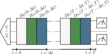
Figure 3: A schematic representation of Eq. 26, showing how the initial density matrix is subsequently multiplied by the propagators of each noise. What is not included in the figure is the fact that due to the non-Markovian component the result has to be averaged over a large number of realizations of $\mathcal{U}_{N}$.

In order to simplify the evolution we will first vectorize the density matrix of the full system, so that the operator $\hat{\rho}$ is transformed into a vector $\hat{\rho}\rightarrow|\rho\rangle\rangle$, and the more general master equation Eq. III.2.1 in Lindblad form is reduced to

$$\frac{\mathrm{d}}{\mathrm{d}t}|\rho(t)\rangle\rangle=\mathcal{L}|\rho(t)\rangle\rangle.$$ (20)

The form of the superoperator $\mathcal{L}$ then depends on the exact vectorization employed. Perhaps the simplest method is to stack the rows of the density matrix, which results in the Liouvillian superoperator $\mathcal{L}$ with the matrix form

$$\mathcal{L}=-i\left(\hat{H}\otimes\mathbb{1}-\mathbb{1}\otimes\hat{H}\right)$$

$$+\sum_{a,b}\Gamma_{1}^{ab}\left(\hat{C}_{ab}\otimes\hat{C}_{ab}^{*}-\frac{1}{2}\left[\hat{C}_{ab}^{\dagger}\hat{C}_{ab}\otimes\mathbb{1}+\mathbb{1}\otimes\hat{C}_{ab}^{\mathrm{T}}\hat{C}_{ab}^{*}\right]\right).$$ (21)

Once we add the stochastic contribution due to $1/f$ noise from Eqs. 8 and 16 to the evolution, we are forced to solve a master equation a large number of times with different realizations of the classical stochastic process. However, we can make use of the fact that for all practical purposes, the noise in the system is weak, and the evolution can be separated into disjoint parts [73].

We take this into account by discretizing the evolution into smaller time steps $\Delta t$, and approximating each time step with a first order truncated propagator. More formally, since the general solution to Eq. 20 with a time dependent $\mathcal{L}(t)$ can be written in terms of a generalized propagator $\mathcal{U}(t_{2},t_{1})$

$$|\rho(t)\rangle\rangle=\mathcal{U}(t,0)|\rho(0)\rangle\rangle,$$ (22)

we can further decompose the superoperator $\mathcal{L}(t)=-i\mathcal{G}(t)-i\mathcal{N}(t)+\mathcal{D}(t)$ into three separate parts:

• $\mathcal{G}(t)$ - representing the closed system dynamics of the system corresponding to the superoperator form of the Hamiltonians in Eq. 1 or III.2.

• $\mathcal{N}(t)$ - corresponding to a single realisation of the classical $1/f$ noise process from Eqs. 8 and 16.

• $\mathcal{D}(t)$ - corresponding to the non-unitary dynamics of any jump operators in the Lindblad equations 6 and III.2.1.

We can proceed to write down the formal solution of Eq. 20 with a Dyson series expansion

$$\mathcal{U}(t,0) =\prod_{n=0}^{\lfloor t/\Delta t\rfloor}\mathcal{U}([n+1]\,\Delta t,n\,\Delta t)$$ (23)

$$=\prod_{n=0}^{\lfloor t/\Delta t\rfloor}\left[\mathbb{1}+\int_{n\,\Delta t}^{(n+1)\,\Delta t}\mathrm{d}t^{\prime}\mathcal{L}(t^{\prime})+\int_{n\,\Delta t}^{(n+1)\,\Delta t}\mathrm{d}t^{\prime}\int_{n\,\Delta t}^{t^{\prime}}\mathrm{d}t^{\prime\prime}\mathcal{L}(t^{\prime})\mathcal{L}(t^{\prime\prime})+\cdot\cdot\cdot\right]$$ (24)

$$=\prod_{n=0}^{\lfloor t/\Delta t\rfloor}\left[\mathcal{U}_{G}([n+1]\,\Delta t,n\,\Delta t)-i\int_{n\,\Delta t}^{(n+1)\,\Delta t}\mathrm{d}t^{\prime}\mathcal{N}(t^{\prime})+\int_{n\,\Delta t}^{(n+1)\,\Delta t}\mathrm{d}t^{\prime}\mathcal{D}(t^{\prime})+\cdot\cdot\cdot\right]$$ (25)

$$\approx\prod_{n=0}^{\lfloor t/\Delta t\rfloor}\mathcal{U}_{G}([n+1]\,\Delta t,n\,\Delta t)\mathcal{U}_{N}([n+1]\,\Delta t,n\,\Delta t)\mathcal{U}_{D}([n+1]\,\Delta t,n\,\Delta t).$$ (26)

In the second to last step we have replaced the linearized propagator with the full propagator of the unitary generator $\mathcal{G}(t)$. This is done since it significantly lowers the error of the expansion as the magnitude of the elements of the matrix form of $\mathcal{G}(t)$ is much larger compared to the noise generators $\mathcal{N}(t)$ and $\mathcal{D}(t)$. The leading error terms of a single step with duration $\Delta t$ are therefore $\propto\int_{n\,\Delta t}^{(n+1)\,\Delta t}\mathrm{d}t^{\prime}\int_{n\,\Delta t}^{t^{\prime}}\mathrm{d}t^{\prime\prime}\left[\mathcal{G}(t^{\prime})\mathcal{D}(t^{\prime\prime})+\mathcal{G}(t^{\prime})\mathcal{N}(t^{\prime\prime})+\cdot\cdot\cdot\right]$, resulting in a global evolution error of $\mathcal{O}(\Gamma\omega T\Delta t)$, where $\Gamma$ is either the pure dephasing or amplitude decay rate, $\omega$ is the largest frequency of the system, $T$ is the duration of the simulation and $\Delta t$ is the duration of a single time step. While the magnitude of the effect of the noise is of the order of $\varepsilon\sim\Gamma_{1}T$ for amplitude decay and $\varepsilon\sim(\Gamma_{\phi}T)^{2}$ for the $1/f$-noise, this means that for accurate results $\omega\Delta t\ll\varepsilon$.

The formula in Eq. 26 basically splits the evolution first into a large number of small timesteps and each time step into a separate contribution of each environmental noise source. In the last line we have also used the full propagator for this noise, instead of the approximate linearized form. This is done in order to avoid unphysical properties of the density matrix.

We mention here also, that splitting the noisy and unitary evolutions is a very common approximation when simulating [74] and benchmarking [27, 75] current noisy devices, even though the error scaling is not very favourable. Here we have gone one step further, by also including the effect of the noise during the gate operation.

The main computational advantage of this is that the set of propagators of the unitary and Lindblad dynamics $\mathcal{U}_{G}$ and $\mathcal{U}_{D}$ are always identical, while the generators $\mathcal{U}_{N}$ depend on each trajectory of the $1/f$-noise we are considering. This means that instead of solving the master equation for each trajectory, we just need to generate the propagators $\mathcal{U}_{G}$ and $\mathcal{U}_{D}$ by propagating $D^{2}$ linearly independent states, where $D$ is the dimension of the system. Since the $1/f$ noise acts on the eigenbasis of the system, we need to diagonalize the Hamiltonian once per each time step and afterwards the exponentiation of the matrix is trivial. Typically we want to average over approximately $N_{\mathrm{traj}}\sim 1000$ trajectories, with a system of dimension $D$. Using $N_{\Delta t}=\lfloor T/\Delta t\rfloor$ time steps, the complexity of the evolution is:

1. Propagate $D$ linearly independent pure states to obtain the generators $\mathcal{U}_{G}$, corresponding to the white dotted area in Fig. 3

2. Propagate $D^{2}$ linearly independent states to obtain the generators $\mathcal{U}_{D}$, corresponding to the blue diagonal patterned area in Fig. 3.

3. Multiply the propagators $\mathcal{U}_{G}$ and $\mathcal{U}_{D}$, corresponding to $N_{\Delta t}$ multiplications of $D^{2}\times D^{2}$ matrices.

4. Diagonalize the Hamiltonian of the system at each time step, corresponding to $N_{\Delta t}$ diagonalizations of a $D\times D$ matrix.

5. Generate the propagators $\mathcal{U}_{N}$, corresponding to the green area in Fig. 3, by simple numerical integration in the eigenbasis and then transform the generator into the correct frame, resulting in 2 matrix multiplications of size $D\times D$ per time step, all together $2N_{\Delta t}$ matrix multiplications per trajectory.

6. Once all the propagators are generated, we need to multiply the initial state at each time step with the precomputed double propagator $\mathcal{U}_{G,D}$ and then with the corresponding propagator $\mathcal{U}_{N}$, meaning that we need to multiply a $D^{2}\times D^{2}$ matrix with a $D^{2}$ dimensional vector twice for each trajectory.

The most numerically difficult steps depending on the exact size of the system are the matrix multiplications in step 3. with a complexity of $\mathcal{O}(N_{\Delta t}D^{6})$ and the actual propagation in step 6. with complexity $\mathcal{O}(N_{\mathrm{traj}}N_{\Delta t}D^{4})$.

IV.3 Measurement

We assume standard dispersive measurements of the transmons in the computational subspace. Even though the same setup could also accommodate the readout of the higher excited states, this readout is typically not calibrated and we assume we have no access to it. Additionally, as mentioned previously, the coupler is not connected to any readout resonator. In the more general two-qubit case, the probability distribution of measuring the state $k$ is given by

$$P(k|\hat{\rho})=\frac{\mathrm{tr}\left\{\hat{P}_{k}\hat{\rho}_{q}\right\}}{\mathrm{tr}\left\{\hat{\rho}_{q}\right\}}.$$ (27)

Where the density matrix $\hat{\rho}_{q}$ is defined in the computational subspace, meaning that it is extracted from the density matrix of the full system $\hat{\rho}$. This procedure is described in the following section V.1 in more detail. Equivalently, also the projector $\hat{P}_{k}$ is defined in the computational subspace.

The normalization in Eq. 27 is needed due to the presence of leakage to the excited states of the transmon, so that the probability distribution $P(k|\hat{\rho})$ is normalized. Once the probability distribution is obtained, we sample $N_{\mathrm{shots}}$ results from it, in order to describe the finite sampling effects. After this procedure we obtain a vector of probabilities of measuring each state (or bit string) $\mathbf{P}(\hat{\rho})=(P(00|\hat{\rho}),P(01|\hat{\rho}),P(10|\hat{\rho}),P(11|\hat{\rho}))^{T}$.

As readout errors in current hardware are large and unavoidable, we model them by transforming the obtained vector of probabilities with a misclassification matrix of the form

$$\tilde{P}(k|\hat{\rho})=\sum_{i\in\{00,01,10,11\}}P(k|i)P(i|\hat{\rho}),$$ (28)

together with the preservation of probability $\sum_{k}P(k|i)=1$.

V Error Budgets of Quantum Gates

V.1 Gate performance measure

The first step in benchmarking a quantum gate is to define a performance measure, which is typically a distance measure between the desired and observed outputs of the gate. The most common measures are typically state or process fidelities, trace distance or diamond norms [76].

Since the simulations are based on state propagation, we choose to examine the gate performance in terms of the averaged state fidelity defined as

$$\bar{\mathcal{F}}=\frac{1}{N_{\psi}}\sum_{\psi}\mathcal{F}(\,\mathcal{E}\left[|\psi\rangle\langle\psi|\right]\,,\,U_{id}|\psi\rangle\langle\psi|U_{id}^{\dagger}\,),$$ (29)

where $U_{id}$ represents the unitary of the gate we are trying to implement and $\mathcal{E}[\cdot]$ is the quantum dynamical map of the noisy evolution corresponding to the chosen gates. The average should be taken over a set of states $\{|\psi\rangle\}$ which is close to the Haar random measure.

The state fidelity is defined as

$$\mathcal{F}(\hat{\rho},\hat{\sigma})=\left|\mathrm{tr}\sqrt{\sqrt{\hat{\rho}}\hat{\sigma}\sqrt{\hat{\rho}}}\right|^{2},$$ (30)

so that if one of the density matrices $\hat{\rho}$ or $\hat{\sigma}$ corresponds to a pure state, the state fidelity is the module squared of the overlap of the density matrix with the pure state.

However, the full Hilbert space of the hardware is much larger than the computational basis, meaning that it is not straightforward to reduce the whole system to its computational basis. Moreover, this is relevant also for the description of the measurement procedure in Eq. 27.

In the case of a single qubit it is straightforward to define a qubitized density matrix in the computational subspace, by simply considering

$$[\hat{\rho}_{\mathrm{comp}}]_{ij}=\langle\phi_{i}|\hat{\rho}|\phi_{j}\rangle,$$ (31)

where we consider the set of computational basis states for the single qubit case as $|\phi_{i}\rangle\in\{|0\rangle,|1\rangle\}$. We note here that such a definition of the qubitized density matrix $\hat{\rho}_{\mathrm{comp}}$ has trace less than one, i.e. $\mathrm{tr}\left\{\hat{\rho}_{\mathrm{comp}}\right\}\leq 1$, which is due to leakage outside of the computational subspace. We do not enforce the normalization when assessing the performance, meaning that the value of the fidelity is limited to the trace of the extracted computational subspace density matrix. Since the original matrix $\hat{\rho}$ is positive semi-definite it follows that also $\hat{\rho}_{\mathrm{comp}}$ is positive semi-definite, as it is defined as a principal submatrix of $\hat{\rho}$ [77]. It is also obvious that by this definition the qubitized density matrix is hermitian. If also the normalization is taken into account, such a qubitized density matrix is completely physical.

The above definition can be easily extended to the multi-qubit case with couplers by considering computational states where the coupler is not excited, namely $|\phi_{i}\rangle\in\{|\widetilde{000}\rangle,|\widetilde{001}\rangle,|\widetilde{100}\rangle,|\widetilde{101}\rangle\}$, with the ordering qubit 1, coupler, qubit 2. We stress here again that the computational states are given by the eigenstates of the multi-qubit Hamiltonian and identified via the maximum overlap rule, which is why we have denoted these Hamiltonian eigenstates with a tilde.

However, there is also a different definition of the qubitized density matrix in this case, which is closer to the actual measured state, if one had access to it. Since we cannot probe the coupler states in any way, it would make sense to trace out the coupler degrees of freedom and then restrict the Hilbert space as in Eq. 31, which would result in a slightly different definition. By this definition, for the two-qubit gate with one coupler, the qubitized density matrix is computed by

$$[\hat{\rho}_{\mathrm{exp}}]_{ij}=\langle\phi_{i}|\mathrm{tr}_{C}\left\{\hat{\rho}\right\}|\phi_{j}\rangle.$$ (32)

The same arguments as in the previous definition still hold to show that this density matrix is physical. The full density matrix is first transformed into the eigenbasis of the full Hamiltonian and afterwards the trace over the coupler states is performed. The states $|\phi_{i}\rangle$ now no longer contain the coupler degrees of freedom, but are still defined in the Hamiltonian eigenbasis, and are therefore given by $|\phi_{i}\rangle\in\{|\widetilde{00}\rangle,|\widetilde{01}\rangle,|\widetilde{10}\rangle,|\widetilde{11}\rangle\}$.

While the latter definition from Eq. 32 might be closer to the experimental measurement, we define the fidelity of an operation with the first definition from Eq. 31, which takes into account the fact that any leakage into the couplers excited states is undesired, since it may corrupt subsequent gate operations.

When considering contributions of individual error sources we limit ourselves to the effects of a single error source being present. This means that we do not independently simulate the performance of the gate for arbitrary combinations of errors, which would also take into account any potential interplay between them.

V.2 Individual error source contributions

We have shown in the previous section that many of the error sources affecting quantum gates may be non-Markovian or time dependent, meaning that also the contribution of such an error source is time or history dependent and cannot be condensed into a single number.

A gate performance measure that would take into account such effects has therefore not yet been defined and is also out of the scope of this work.

Instead, we choose to monitor the evolution of the averaged state fidelity after applying a series of gates. For non-unitary Markovian noise sources such a contribution will increase linearly and for coherent errors quadratically provided the error is small. More complex errors might display more complex behaviour, with non-monotonic decays being associated with non-Markovianity [21].

V.3 Examples with typical parameters

Now that we are able to simulate quantum gate operations with more realistic noise models, we can examine the effect of individual error sources on a series of quantum gates.

V.3.1 Single-Qubit Gates

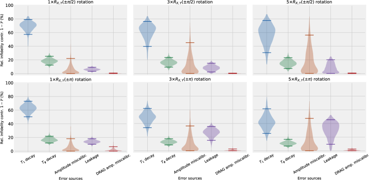
Figure 4: The distributions of relative infidelity contributions of different error sources with typical experimental parameters. The relative error contribution of an error source is obtained by simulating the dynamics of a Gaussian DRAG pulse with $\sigma=4$ ns and $t_{g}=16$ ns, with each error source individually and then normalizing with respect to all of the other error contributions. Top row: Relative infidelity contributions of $\pi/2$ rotations microwave pulses around the $x$ or $y$-axes, calculated by repeating the gate one, three or five times (columns). Bottom row: The error contributions of microwave pulse $\pi$ rotations. We consider the same parameters for both $\pi$ and $\pi/2$ rotations, which are listed in Table 1. The error sources which are not listed were found to have a negligible effect on the infidelity. The horizontal bars represent the 5th and 95th percentiles of each distribution.

Here we analyse the average effect of the error sources of single qubit gates. The error sources we have considered have been listed in Sec. III.1.

We define the infidelity contribution of an error source by simulating the effect on an ideal system with only such single error source, and evaluating the state averaged fidelity from Eq. 29.

Since the parameters of the qubit as well as the noise differ between chips and also qubits on the same chip, we must look at a large range of possible parameters. In order to do so we sample the noise parameters from independent Gaussian distributions with realistic standard deviations and mean values obtained from the current literature. The range of parameters as well as the references considered is summarized in Table 1, which is divided into three sets:

• The first set of parameters in Table 1 refer to the single transmon Hamiltonian in Eq. 1 and mainly the value of the anharmonicity $\alpha$ is responsible for the contribution of the leakage of the pulse to the infidelity. We mention here that there are other errors associated with the DRAG pulse, like the breaking down of the RWA as well as phase errors, however in our simulations these are always observed to be much smaller compared to the leakage into the second excited state.

• The second set of parameters concern the most important errors of the system. We note here that while a finite temperature $T_{eff}$ with both heating and decay processes is taken into account in the amplitude damping simulations, the heating processes have a very small contribution to the infidelity of the gate, due to the relatively low temperature. We do not consider state preparation errors as part of the gate infidelity in order to make a clear distinction between these effects. When evaluating the effect of $T_{1}$, $T_{\phi}$, $\epsilon_{A}$, we consider an idealized two-level system where the rotating wave approximation (RWA) holds, while when considering the effect of the DRAG pulse or a miscalibration of the second quadrature $\epsilon_{\beta}$ a three-level system without RWA is used. In the case of $\epsilon_{\beta}$ the obtained infidelity is subtracted from the infidelity of the full DRAG pulse with ideal parameters in order to isolate the effect of this miscalibration.

  The pure dephasing due to Markovian white noise is characterized by the decay time $T_{\phi}$. This timescale is much longer compared to the $T_{1}$ decay, since most of the noise in the pure dephasing has a low-frequency $1/f$-like spectrum and is simulated as a non-Markovian process.

  The errors in the miscalibration of the pulse parameters from Eq. 3 are characterized by the values $\epsilon_{A}$ and $\epsilon_{\beta}$ in Eqs. 9 and 10. We mention here that using the calibration procedures presented in Ref. [64], the amplitude of the pulse is set for either a $\pi$ or equivalently $\pi/2$ rotation, and typically only one of the two rotations will exhibit a larger error in the amplitude. In order to cover both cases, we consider a smaller error than reported in Ref. [66], but comparable to the values from Ref. [67] for both gates.

  We can see from Table 1 and Fig. 4 that even a relatively large error in the DRAG amplitude $\epsilon_{\beta}$ does not result in a drastically decreased performance. This is of crucial importance also when considering the effects of the drive non-linearity on one single gate. What is meant by drive non-linearity in this context is the fact that the shape of the pulse is slightly compressed (smaller than expected) at higher amplitudes. This effect will mean that the quadrature with the larger amplitude is flattened, and therefore strictly speaking the smaller quadrature is no longer a perfect derivative. However since we are not especially sensitive to errors in the amplitude of the derivative, we are also not especially sensitive to the non-linearity of the drive.

• The last set of parameters was included in the simulation, however their infidelity contributions were found to be much smaller compared to the other errors. The frequency detuning $\delta\omega=\omega-\omega_{d}$ due to the drift of the qubit parameters is simply too small, unless we consider a qubit which has not been calibrated for a very long time. The magnitude of the effect on $N$ gates with duration $t_{g}$ can be estimated by the value $(N\delta\omega\,t_{g})^{2}$.

  What is more surprising is that the long-time correlated $1/f$ noise has a negligible contribution even though the associated decay times were assumed to be much shorter compared to the Markovian pure dephasing $T_{\phi}$. The reason for this is two-fold, firstly, the shape of the decay due to such noise is not exponential but rather closer to a Gaussian curve, therefore it decays more slowly on shorter timescales [78]. Secondly, the microwave driving of the transmon acts as dynamical decoupling, as was previously described in Ref. [79].

Table 1: Table of parameters used to generate the plots in Fig. 4. These values are typical in state of the art devices.

	Parameter	Mean	Std. deviation	Units	Ref.
III.1	$\omega$	4.5	0.05	$2\pi$ GHz	[4, 3, 80]
III.1	$\alpha$	-200	7.5	$2\pi$ MHz	[4, 3, 80]
III.1.1	$T_{1}$	35	7	$\mu$s	[4, 3, 80]
III.1.2	$T_{\phi}$	65	7.5	$\mu$s	[4]
III.1.4	$\epsilon_{A}$	0	0.5	Deg.	[66, 67]
III.1.4	$\epsilon_{\beta}$	0	2	%	[64]
III.1.4	$\delta\omega$	0	10	kHz	[29]
III.1.3	$T_{\phi}^{1/f}$	15	2.5	$\mu$s	[4, 3]
III.1.1	$T_{eff}$	45	5	mK	[52, 53, 54]

Fig. 4 shows the typical behaviour where a single gate infidelity is typically $T_{1}$-limited, however after a number of repetitions of the gate this might not be the case anymore, as the quadratic scaling of coherent errors stemming from the amplitude miscalibration slowly overcome the $T_{1}$ contribution in some cases. Additionally, we can see that even an optimized DRAG pulse still results in significant leakage for larger rotation angles. While one might be able to use standard techniques to obtain the single gate infidelity corresponding to the first column of Fig. 4, this shows that a single number must be carefully interpreted and the characteristics of the noise better understood if we want to make statements about the performance of a larger sequence of gates or an algorithm [75].

We note here that in many cases, such as for example the qubit frequency $\omega$ from Eq. 1, the exact values depend on the design of each specific chip. In case we are interested in a different set of parameters, the general rule that applies to all of the distributions plotted in Fig. 4 is that increasing the mean value of any error will shift the mean of the distribution towards a larger contribution and increasing the uncertainty of the parameter will increase the width of the distribution. As long as one considers parameter guesses based on bell-shaped curves the shapes of the distributions will not change significantly.

V.3.2 Two-Qubit Gates

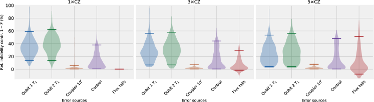
Figure 5: The distributions of relative infidelity contributions of different error sources with typical experimental parameters of a two-qubit non-adiabatic CZ gate. A 16 ns idling time is introduced after each application of the CZ gate in order to mimic the performance in an algorithm, since 16 ns is the duration of a single-qubit gate analyzed in this work. The relative error contribution of an error source is obtained by simulating the dynamics of a flattop-Gaussian pulse from Eq. 13 with $\sigma=5$ ns and $\tau_{b}=2\sqrt{2}\sigma$. Since the transmons in the system have different parameters for each realization, the time $\tau_{c}$ and amplitude $A$ are numerically optimized for each individual instance, and is typically close to the value of 30 ns. The relative error contributions are obtained by simulating the full system with each error source individually and the normalizing the values, identically as in Fig. 4. The category Control represents the inherent control errors associated with the specified pulse shape, finite time resolution of the electronics $\epsilon_{\tau_{c}}$ and amplitude uncertainty $\epsilon_{A}$. The error sources considered and corresponding parameter ranges are listed in Table 2. The error sources which are not listed were found to have a negligible effect on the infidelity. The horizontal bars represent the 5th and 95th percentiles of each distribution.

A similar analysis can be performed for the two-qubit CZ-gate. The parameters and the uncertainties we consider are shown in Table 2. However, in the case of the two-qubit gate, we always simulate the full system comprised of three transmons for two reasons. Firstly, the gate is diabatic and the population must leave the computational subspace, and secondly constructing any reduced models with smaller Hilbert spaces might warrant unrealistic approximations. Since the infidelity of the gate with optimized parameters can be comparable to the infidelity of certain error sources, the infidelity of the optimized pulse is subtracted from the infidelity obtained by adding an individual error source. This is supported by the results from Refs. [73, 81], where it was shown that in the case of weak noise, the infidelity contribution is independent of the unitary dynamics.

Table 2: Table of parameters used to generate the plots in Fig. 5. These values are typical in state of the art devices.

	Parameter	Mean	Std. deviation	Units	Ref.
III.2	$\alpha_{Q_{1}}$	-194	10	$2\pi$ MHz	[9]
III.2	$\alpha_{C}$	-100	5	$2\pi$ MHz	[9]
III.2	$\alpha_{Q_{2}}$	-187	10	$2\pi$ MHz	[9]
III.2	$\beta_{Q_{1}C},\beta_{Q_{2}C}$	$15$	$0.75$	$10^{-3}$	[9, 13]
III.2	$\beta_{Q_{1}Q_{2}}$	$1$	$0.05$	$10^{-3}$	[9, 13]
III.2.2	$\omega_{C}^{\mathrm{max}}$	6.9	$0.15$	$2\pi$ GHz	[9, 13]
III.2.1	$T^{Q_{1}}_{1},T_{1}^{C},T_{1}^{Q_{2}}$	15	5	$\mu$s	[10, 9]
III.2.2	$T^{Q_{1}}_{1/f},T_{1/f}^{Q_{2}}$	15	5	$\mu$s	[10, 9]
III.2.2	$T^{C}_{1/f}$	1.5	0.3	$\mu$s	[10, 9]
III.2.3	$\epsilon_{A}$	0	0.02	$2\pi$ GHz
III.2.3	$\epsilon_{\tau_{c}}$	0	0.2	ns
III.2.4	$A_{n}$	1	0.5	%	[9]
III.2.4	$\tau_{n}$	300	100	ns	[9]
III.2.2	$T^{Q_{1}}_{1/f},T^{Q_{2}}_{1/f}$	15	5	$\mu$s	[10, 9]

As an additional comment to the parameters presented in Table 2, we have added the maximal frequency of the coupler $\omega_{C}^{\mathrm{max}}$, which is relevant when computing the flux dispersion $\partial\omega_{C}/\partial\mathrm{\Phi}$ during the flux pulse, as seen from Eq. 7. Otherwise the coupler is idled at the idling point where there is no residual ZZ interaction between the computational states.

We represent the distributions of the relative infidelity contributions for two-qubit gates in Fig. 5. One interesting result observed is that in the infidelity contribution can be actually negative. This corresponds to the situation when the fidelity with the error source is higher compared to the full optimized (but imperfect) unitary evolution, as is the case when considering flux distortions. Since the non-adiabatic implementation of the gate is based on the Rabi oscillation of the computational $|11\rangle$ and non-computational $|02\rangle$ states, there are two conditions for a high fidelity gate, first of which is that all the population after the gate operation returns to the $|11\rangle$ state and secondly that the population returns with the correct conditional phase. Furthermore, these two points have to coincide for a realistic gate duration. That is why we often make a trade-off between highest achievable fidelity and gate duration. Connecting this discussion to the effect of the flux tails, since the flux tail will offset the idling point of the coupler frequency which will accumulate an additional conditional phase, as well as effectively shift the amplitude of the pulse, it may compensate e.g. for some error in the original conditional phase. For example, consider a CPHASE gate with a conditional phase of $\pi-\varepsilon$, in some cases the idling conditional phase due to the flux tails will compensate for the small offset $\varepsilon$ resulting in a better perceived gate performance, on the scale of a couple of gates. If more gates are repeated, the effect of the flux distortions eventually outweighs any potential benefits, provided the correlation time $\tau_{n}$ is long enough.

We argue that in the two-qubit gate case, it does not make sense to separate the effects of the small error in pulse amplitude $\epsilon_{A}$ and duration $\epsilon_{\tau_{c}}$, due to the fact that most times the magnitude of these errors is smaller compared to the inherent error of the pulse shape considered here. Secondly, in an experimental setting, typically the finite precision of the electronics resulting in a finite $\epsilon_{\tau_{c}}$ means that even if better parameters do exist, they are not achievable with realistic equipment and the noise in the experiment.

Similarly to Fig. 4, also Fig. 5 shows the same behaviour, where $T_{1}$ induced error is dominant on the scale of a single gate, but as more operations are performed, other errors start to contribute more. Because of the poor coupler coherence times there is also a small contribution of the $1/f$ flux noise in the coupler, mainly due to the Gaussian shape of the decay. Moreover, the effect of the flux tails is observed to become even more dominant as more gates are performed and more distortion is accumulated.

V.4 Experimental reconstruction

In the previous section we have seen how the contributions of different error sources vary considerably depending on the value of a large number of parameters. Now we are able to also perform the budgeting procedure described in Sec. V.4 on both single and two-qubit gates.

V.4.1 Quantifying the Performance

In order to quantify the performance of our regression, we use the coefficient of determination [82], often referred to as the $R^{2}$ score, defined as

$$R^{2}=1-\frac{\sum_{i}(y_{i}^{\mathrm{pred}}-y_{i}^{\mathrm{true}})^{2}}{\sum_{i}(y_{i}^{\mathrm{pred}}-\bar{y}^{\mathrm{true}})^{2}},$$ (33)

where $y_{i}^{\mathrm{pred}}$ is the model prediction and $y_{i}^{\mathrm{true}}$ is the correct value. In our case, the values $y_{i}$ refer to infidelity contribution of a single error source to the infidelity of a single gate series, where the superscript refers to whether this is the value predicted by our model (pred) or the actual correct value (true). We can then calculate the $R^{2}$ for each gate series and error source independently.

The sum runs over a testing set of size $n$ over which we define our performance. In our case the testing set consists of simulated experiments together with their corresponding error budgets that were not used in the training step of the GPR. The average of the values in the testing set is denoted as $\bar{y}^{\mathrm{true}}=1/n\sum_{i}y_{i}^{\mathrm{true}}$. Such a definition has a clear interpretation, in terms of the amount of variance in the sample the model is accounting for.

The value can be interpreted as $R^{2}=1$ being the perfect score, while $R^{2}=0$ means that our predictions are as good as the outputs of a model that always predicts the mean value of the training sample, irrespective of the input. While some information (the mean and standard deviation of the training sample) can still be deduced if $R^{2}=0$, when $R^{2}<0$, the model is completely unreliable, with the lower bound depending also on the testing set. In the latter case the performance can be compared to a random guess.

We have chosen this metric for a number of its favourable properties. First of all, since the score is normalized with respect to the variance, we will not be overestimating the performance of our model when the variance is small. Imagine that an error source has a sizeable but constant contribution, unless we are more accurate compared to the variance of this error source, our $R^{2}$ score will be small. In this case, metrics such as mean absolute or squared errors might be low, thus falsely overestimating the model performance.

Secondly, since this metric is typically constrained between 0 and 1 it enables us to compare the performance even when the values are very different, i.e. in the case of comparing the infidelity contributions of a single gate or 9 gates, the absolute values, and by extension the mean absolute or squared error values, are very different, while both $R^{2}$ scores are in a comparable range.

Additionally, compared to other frequently used metrics, such as the mean absolute error, mean squared error, root mean squared error and mean absolute percentage error, the $R^{2}$ metric was shown to have less interpretability limitations. Additionally it was shown to also be more truthful and informative compared to the symmetric mean absolute percentage error [83].

However since we are interested in different error sources, we compute the $R^{2}$ score for each error source, and determine the final performance with the variance weighted $R^{2}$ score, defined as

$$R^{2}=\frac{\sum_{k\in\{T_{1},T_{\phi},\epsilon_{A},\dots\}}\sigma_{k}^{2}R_{k}^{2}}{\sum_{k\in\{T_{1},T_{\phi},\epsilon_{A},\dots\}}\sigma_{k}^{2}}.$$ (34)

In other words, the $R^{2}$ is calculated for each feature independently, since we use a separate GPR model for each feature. A weighted average, with the weights determined by the variance of each feature, defined as $\sigma^{2}=1/n\sum_{i}(y_{i}^{\mathrm{true}}-\bar{y}^{\mathrm{true}})^{2}$ in the test sample, is then used to asses the performance over all of the error sources.

V.4.2 Single Qubit Gates

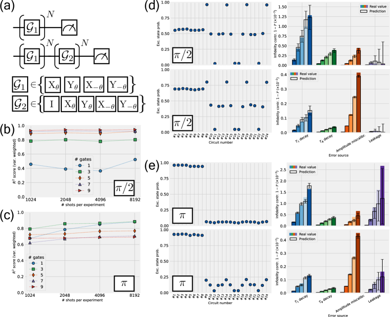
Figure 6: Examples of reconstructing the error budgets of single-qubit gates with realistic experimental parameters. (a) Circuits used as an input for the algorithm, where $\theta$ is equal to either $\pi$ or $\pi/2$, depending on which gate we are interested in. We use all $24=N_{\mathcal{G}_{1}}+N_{\mathcal{G}_{1}}\times N_{\mathcal{G}_{2}}$ possible combinations of $\mathcal{G}_{1}$ and $\mathcal{G}_{2}$. In the data presented above, $N=25$, and the initial state is the thermal ground state as described in Sec. IV.1. (b) Performance of the budgeting on a test set of 40 $\pi/2$ rotation gates with different error parameters, quantified in terms of the $R^{2}$ score, weighted by the variance of each feature. Different shapes correspond to the accuracy of the error source contribution predictions to the averaged state infidelity of a series of gates. (c) Similarly as in (b), except for the $\pi$ rotation. (d) Two input-output pairs of the testing set for the $\pi/2$ rotation, with the input on the left and the output on the right, for different examples. The input data is the probability of measuring the excited state population, together with a finite measurement error and finite number of shots, as described in Sec. IV.3. We have only included the most dominant error sources from Fig. 4 in the outputs, and each of the error sources has 5 different columns, corresponding to the infidelity contribution to 1, 3, 5, 7 or 9 gates (in this order). The empty columns represent the predictions of the trained Gaussian Process Regressor model, together with the corresponding uncertainties and the filled columns are the correct value. In an ideal scenario, the filled and empty columns would directly coincide. (e) Identically as in (d), except for the $\pi$ rotation.

We first test our devised method for error budgeting on single qubit $\pi$ and $\pi/2$ rotations. We make no distinction between $X$ or $Y$ rotations, or positive or negative values of the rotation angle, since the error source contributions are expected to remain the same. Actually the only difference between these operations are the phases of the harmonic drive of the pulse in Eq. 2.

We start by generating a large set of simulations of potential experiments with the parameters from Table 1. Additionally, we also consider a random finite temperature of the qubit, as described in Sec. III.1.1 and IV.1, $\mu[T_{\mathrm{eff}}]=45$ mK with a spread of $\sigma[T_{\mathrm{eff}}]=5$ mK [52]. For the single-qubit case, we consider additional random measurement errors $P(0|1)=2.5\%\pm 0.8\%$ and independently $P(1|0)=1.0\%\pm 0.5\%$ as seen in Eq. 28. The uncertainty represents one standard deviation of the data. These numbers correspond roughly to the measurement infidelity already demonstrated in a large-scale device in Ref. [4] and significantly better readout performance was demonstrated in Ref. [84].

Each of the parameters is then sampled randomly from a Gaussian distribution and used to simulate a number of noisy experiments. These experiments are shown in Fig. 6(a). The main idea is to repeat the gate of interest a large number of times in order to amplify all the relevant noise processes. Different combinations of gates are there in order to increase the total amount of information, i.e. a combination of positive and negative rotations will cancel the effects of gate amplitude errors. Since this choice of experiments is most likely not optimal, we believe that there is still room for improvement in the future.

After the sample of approximately 500 simulations with the corresponding error source contributions is obtained, this data set is split into a large training set, containing approximately 90 % of the samples, and a small testing set, containing the rest of the samples, which we use to test the performance of the predictions. Each input and output is then linearly rescaled to mean zero and a standard deviation of one, before a separate Gaussian Process Regressor is trained to predict each single error source contribution, for each number of gates individually. The training is described in more detail in Appendix A.

After the training, the performance of the GPR predictions on the test set is evaluated. The results with two input-output pair examples are shown in Fig. 6(b-e).

Looking specifically at 6(b) and (c), we can see that even low shot numbers are typically enough to obtain good performance. Estimating the time needed to acquire one single shot to approximately 0.5 ms with 4000 shots, the time needed to perform the actual experiment is approximately $0.5\times 4000$ ms $\sim 1$ minute. Here we have implicitly assumed that the time needed to evaluate one shot is limited by the reset time of the system, which (in case no active reset has been implemented) is typically on the order of a couple $T_{1}$ times. The reason for observing a relatively constant performance versus the number of shots is the fact that the inaccuracy in the measurement errors dominates the inaccuracy due to the finite number of shots.

Finally, 6(d) show in the left panels two typical sets of simulated input values, emulating experimental measurements of the excited state probability for a $\pi/2$ rotation. Fig. 6(e) shows the same for a $\pi$ rotation. In all cases, the right panels show the corresponding infidelity contributions for the main error sources as computed directly from the simulated input (real values, displayed in the filled columns) compared to the ones predicted with our method (prediction, displayed in empty columns), for different number of gates.

As a summary, our results show how a number of circuit outcomes, with low shot numbers and realistic state and readout preparation errors can be used to connect the observed data to a theoretical model of the dynamics, for unitary, non-unitary and non-trace-preserving errors. We are typically able to explain between 70% and 90% of the variance of the sample considered.

V.4.3 Two Qubit Gates

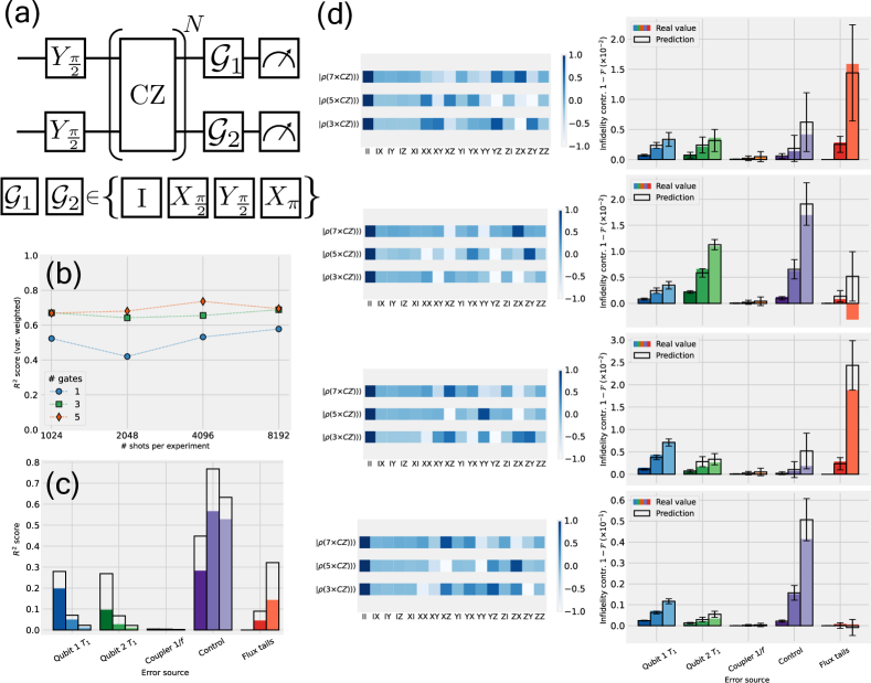
Figure 7: Examples of reconstructing the error budgets of a non-adiabatic two-qubit CZ gate with realistic experimental parameters from Table 2. (a) The circuits used as an input for the budget reconstruction. The initial state is the thermal ground state as described in Sec. IV.1 and two single-qubit gates are used to initiate a superposition state in both qubits, so that all of the elements of the qubitized density matrix are non-zero. The CZ gate is then applied $N$ times, before single-qubit gates are applied, and simple linear inversion state tomography is performed. We use three circuit with $N=3$, $N=5$ and $N=7$ CZ gates. (b) Performance of the budgeting on a test set of 40 CZ gates with different parameters, quantified in terms of the $R^{2}$ score, weighted by the variance of each feature. Different shapes correspond to the accuracy of the error source contribution predictions to the averaged state infidelity of different numbers of gates. (c) The detailed performance of the budget reconstruction for each noise source described in Sec. III.2. The height of the empty columns represents the relative weight of each feature, given by the variance of that contribution in the test sample, as described in Eq. 34. The filled columns represent how good the predictions are, i.e. a completely filled column indicates a perfect score. (d) Four input-output pairs of the testing set for the CZ gate. The input data plotted are the results of simple linear inversion state tomography on states prepared by running the circuits in (a). The density matrices are transformed into Pauli vectors with elements $\left[|\rho\rangle\rangle_{\mathrm{Pauli}}\right]_{i}=\mathrm{tr}\{\hat{\rho}\hat{P}_{i}\}$, where $\hat{P}_{i}$ is the Kroenecker product of two Pauli matrices indicated on the $x$-axis. The inputs also include readout errors. Similarly as in Fig. 6 each of the error sources has 3 different columns, corresponding to the infidelity contribution to 1, 3, or 5 CZ gates (in this order). The empty columns represent the predictions of the trained Gaussian Process Regressor model, together with the corresponding uncertainties and the filled columns are the correct value. In an ideal scenario, the filled and empty columns would directly coincide.

While the budgeting reconstruction algorithm for two-qubit gates follows more or less the same steps compared to the single qubit case, there are slight differences in the implementation. Most notably, the experiments used as the input for the algorithm, shown in Fig. 7(a) must also contain single-qubit gates, since the CZ gate is a diagonal operation and applying it to a system in the ground state will not induce any excitations, which are susceptible to the environmental effects. Therefore we start by creating a superposition state in both qubits after which we apply the entangling operation a number of times. Finally, a second layer of single-qubit gates is performed. This was inspired by the work in Ref. [24], where tomographically reconstructed density matrices were used to find the best non-Markovian description of the system. We perform simple linear inversion state tomography [76], since it is not crucial for our developed technique that the reconstructed density matrices are completely physical, however in the case of worse readout parameters, improving the tomographic reconstruction step might be beneficial. Some examples of the reconstructed density matrices after applying the entangling operation a number of times are shown in Fig. 7(d) in the Pauli vector representation. The reason why the vectors seem so different from each other, even though the fidelity of the gate is not particularly low, is the presence of single-qubit phases, which we have not compensated for.

The readout infidelities and corresponding uncertainties assumed in the results presented in Fig. 7 are the same as for the single-qubit case, namely $P(0|1)=2.5\%\pm 0.8\%$ and independently $P(1|0)=1.0\%\pm 0.5\%$.

Observing the performance of the procedure for the two-qubit gate in Fig. 7(b,c) and the examples in Fig. 7(d), shows a reduced accuracy compared to the single-qubit case. We attribute this to the fact that for the larger system, there is a much larger number of uncertain parameters, e.g. the couplings between the transmons, making it harder for any algorithm to characterize with a very limited amount of data. This is illustrated in Fig. 7(c), where the performance was additionally broken down into scores for each category. While both qubit $T_{1}$ times are modelled in the same way, since the frequency of the second qubit in this model is higher, only the second qubit’s states hybridize strongly with the coupler states. The magnitude of this effect depends strongly on the coupling strength between qubit 2 and the coupler as well as the optimal pulse amplitude, making the whole dependence more complex. Additionally, this means that a part of the qubit 2 decay is a consequence of the amplitude damping of the coupler.

We have also demonstrated that we are able to capture some of the effects of control errors and flux-tails, even though these error sources manifest themselves as unitary, non-unitary and non-TP errors. In order to distinguish between the effects of a single pulse it is crucial to have access to the density matrix of the system at different times of the evolution.

The needed number of shots for the presented accuracy is very similar to the single-qubit case, and remains relatively low, with the estimated experimental time on the scale of minutes.

V.4.4 Cost Comparison

Let us make a more detailed comparison on how the errors from Fig. 7 can be diagnosed without the use of the GPR method outlined in this paper. Ignoring non-Markovian effects, methods such as GST [18] and variants of randomized benchmarking [19, 21] can be used to obtain more accurate benchmarks, however at a much higher experimental cost. To make the comparison more fair, in our analysis we consider the error characterization procedures from Ref. [9] as a baseline, since we can also make the same assumptions about the error sources as in our GPR based procedure.

As a reminder we mention here that the GPR procedure described in this paper, in the case of the two-qubit gate, requires three state tomography experiments, or 48 different circuits.

Table 3: The characterization experiments performed in Ref. [9] that are needed to obtain similar results to Fig. 7, with the same assumptions about the noise.

Error Source	Characterization experiment
Qubit 1 $T_{1}$	$T_{1}$ measurement
Qubit 2 $T_{1}$	$T_{1}$ measurement
Control	State tomography + $f$-state readout
Flux tails	Several Ramsey exp. + SWAP to Coupler

The experiments required for a characterization of the same error sources and a comparable accuracy, but without utilizing the GPR method are listed in Table 3. To further elaborate on the data in Table 3, we assume that a $T_{1}$ experiment with a modest accuracy consists of measuring $\sim$5 circuits, while a single two-qubit state tomography requires 16 distinct circuits and the leakage contribution can be roughly estimated with a single circuit, provided $f$-state readout is available. For the Ramsey experiments needed to evaluate the flux-tail contribution, we can assume that at least $\sim 10$ further circuits need to be measured, as an accurate coupler frequency characterization means that several oscillations must be seen in the experimental data. Further assuming that the coupler frequency after applying a flux pulse is measured at $\sim$5 different delay times in order to estimate the flux-tail magnitude, this brings the minimal total number of distinct circuits needed for the characterization to $\sim 75$, which is approximately a factor of $\sim 1.5$ times more compared to the proposed GPR based procedure.

Additionally, the coupler transmon typically cannot be directly read-out and does not have dedicated drive lines for implementing single-qubit gates. This means that if we want to probe the flux-tail effects on the coupler, an excitation must first be prepared in the computational transmon and then transferred to the coupler with a SWAP-like operation, which needs additional experiments to tune up. The same also applies to the coupler readout. We estimate that this additional calibration, assuming the computational transmon frequency is known from the calibration of single-qubit gates, requires $\sim 25$ more data points. To see this, one should consider that to maximize the population transfer between the computational and coupler transmons, we must tune the coupler to the frequency of the qubit transmon, and let the system interact for a time of approximately $1/g_{2c}$, so that one Rabi cycle is performed. If the frequency of the coupler and duration of the interaction are swept with 5 distinct values each, we arrive at the number $\sim 5\times 5=25$.

Thus, together with the previous steps, this adds up to a total of 100 distinct circuits to run, resulting in a final advantage of more than a factor of $\sim 2$ for the GPR based method.

Not utilizing the GPR method also has additional drawbacks, namely:

1. Once the noise parameters are experimentally obtained, a subsequent simulation of the system with them is needed to evaluate the actual infidelity contributions. Translating the measured uncertainties into fidelity bounds will demand even more simulation time. This means that more time is needed to evaluate the error contributions due to the time required to perform the simulations. The time associated with the classical simulations depends on the complexity of the system and error sources, but in our case it can take up to a couple of minutes, meaning that it is comparable to the time needed to run the experiments on the quantum hardware.

2. The GPR based procedure uses circuit outcomes as inputs and no pulse-level control of the system is needed. Probing any error source affecting the coupler (flux tails, coupler $1/f$, etc.) will always demand pulse-level access due to the aforementioned SWAP-like operation, while this is not necessary for the GPR method.

VI Conclusions

In this work we have demonstrated how different error sources in quantum gates may be pinpointed from experimental data using pulse-level simulations and demonstrated the performance using detailed simulations of superconducting qubits. Unlike traditional system agnostic quantum characterization techniques, we use the fact that we have a model available for the dynamics, which can be used to make educated predictions on the sources of the infidelity of the gate, with a small number of shots needed. We estimate that the proposal requires half as many quantum resources compared to a similar characterization procedure with the same accuracy, and is more flexible, as we have shown how errors resulting in leakage, non-Markovian dynamics and both coherent and incoherent errors can be estimated and even more crucially pinpointed in experiment, with the main bottleneck being the complexity of the noisy gate simulations.

We note that the accuracy of the predictions can be further improved by optimizing the design of input experiments beyond the ones considered in this work.

Because of its low experimental overhead and relative flexibility, the main benefits of our proposed reconstruction procedure will become evident for the error diagnosis of different gates in large scale chips, for example after or before a calibration procedure has been performed. Furthermore, this method can also be extended to co-designed circuits containing computational elements beyond qubits, such as the ones proposed in Refs. [41, 85].

To illustrate the method, we have analyzed the error sources contributing to the infidelity of qubit operations in superconducting quantum architectures. To this aim we have presented what is perhaps one of the most accurate and complete noise models, including realistic descriptions of the environmental, as well as control errors present in current devices. Namely, we consider a realistic non-Markovian description of the pure dephasing dynamics and the non-local effects of the $T_{1}$ decay due to the coupling to an environment of TLSs. We have additionally accurately simulated the effects of control errors due to imperfections in the electronics, which can also in some cases exhibit non-Markovian behaviour, all while keeping the simulation tractable without the use of high performance computing.

With the help of these accurate models, we have demonstrated that when considering the performance of more than a single gate, current state of the art hardware is not necessarily limited by environmental effects such as $T_{1}$ decay, but that control imperfections can be a significant source of error in an algorithm execution. This fact is often hidden when reporting gate fidelities as a performance metric, since the infidelity of a single gate can be dominated by incoherent errors, while the infidelity of a series of gates or an algorithm can be dominated by other error contributions, due to the different scaling of coherent errors. These findings warrant the use of coherent error suppression techniques such as randomized compiling [80] as well as more frequent calibration. Interestingly, we have also found that the non-Markovian nature of $1/f$ flux noise implies that we will often overestimate the effect of the pure dephasing decay on the gate infidelity, if the pure dephasing decay times obtained via Ramsey experiments are used in the estimation. We expect that the results on the average error contribution will improve the current modelling of whole algorithms.

Appendix A Gaussian Process Regression

Before delving into the details of Gaussian Process Regression (GPR), we will start by first defining what a Gaussian Process (GP) is and then show how it can be applied to supervised learning tasks.

However, starting out with the basics, a multivariate Gaussian probability distribution is defined as

$$\mathcal{N}(\mathbf{x},\pmb{\mu},\Sigma)=\frac{1}{(2\pi)^{D/2}|\Sigma|^{1/2}}\exp{\left[-\frac{1}{2}(\mathbf{x}-\pmb{\mu})^{T}\Sigma^{-1}(\mathbf{x}-\pmb{\mu})\right]},$$ (35)

which is completely specified by its mean vector $\pmb{\mu}\in\mathbb{R}^{D}$ and covariance matrix $\Sigma$. The off-diagonal elements of the covariance matrix $\Sigma$ determine the degree of correlation between the elements of the vector $\mathbf{x}=(x_{1},x_{2},...,x_{D})^{T}$. If one were to draw random samples of $\mathbf{x}$ and plot them in pairs of $\{(i,x_{i}),\,1\leq i\leq D\}$, if $\Sigma$ is a diagonal matrix, each element of the vector is drawn independently from the others, at the resulting plot would display one realisation of uncorrelated white noise. On the other hand if $\Sigma$ has large off-diagonal elements, each element of $\mathbf{x}$ is strongly correlated with the others, and the resulting plot reminds us of a smooth function. This intuitive example paves the way to understanding how to use Gaussian processes for supervised learning tasks.

Instead of individually specifying each element of the covariance matrix $\Sigma$, we will always parametrize it in terms of covariance functions $\left[\Sigma\right]_{i,j}=k(\mathbf{x}_{i},\mathbf{x}_{j})$. Furthermore, if $k(\mathbf{x}_{i},\mathbf{x}_{j})$ depends only on the scalar product of the vectors $\mathbf{x}_{i}\cdot\mathbf{x}_{j}$, the function $k(\cdot,\cdot)$ is a kernel function.

An important property of the above distribution is the so-called marginalization property, meaning that if we arbitrarily split a multivariate Gaussian variable vector into two $\mathbf{x}=(\mathbf{x}_{1},\mathbf{x}_{2})^{T}$, both subvectors are also Gaussian distributed, $\mathbf{x}_{1,2}\sim\mathcal{N}(\mathbf{x}_{1,2},\pmb{\mu}_{1,2},\Sigma_{1,2})$, with the relevant submatrix $\Sigma_{1,2}$ [34].

A Gaussian process is a type of stochastic process, defined as a collection of random variables, any finite number of which have a joint Gaussian distribution. It is therefore completely specified by its mean $\pmb{\mu}$ and covariance matrix $\Sigma$. A Gaussian processes model therefore describes a probability distribution over possible functions that fit a set of points [86].

Now focusing on the regression task we wish to tackle, we have access to a number of (possibly noisy) input-output pairs $\{(\mathbf{x}_{i},y_{i})\}$, where $y_{i}=f(\mathbf{x}_{i})+\epsilon$ and $\epsilon$ is an independently and identically distributed Gaussian noise in the observations. Instead of trying to find a single function $f(\mathbf{x})$ that best fits the data, we try to find a probability distribution over the functions that fit the data, and make predictions based on the means of this distribution of functions. Since we have a supervised learning task, we need to incorporate our knowledge of the prior observations.

The regression function defined by Gaussian processes is therefore

$$P(\mathbf{y}|X)=\mathcal{N}(\mathbf{f}|\pmb{\mu},\Sigma),$$ (36)

where $\mathbf{y}=(y_{1},y_{2},\dots,y_{D})$ is a vector of our observations, and $X=(\mathbf{x}_{1},\mathbf{x}_{2},\dots,\mathbf{x}_{D})$ is the ordered matrix of the input vectors corresponding to each observation. We have still included the mean vector $\pmb{\mu}$ although the input data is typically normalized to zero mean. The covariance matrix $\left[\Sigma\right]_{i,j}=\mathrm{cov}\left[f(\mathbf{x}_{i}),f(\mathbf{x}_{j})\right]=k(\mathbf{x}_{i},\mathbf{x}_{j})$ has been parametrized in terms of a kernel function. A typical, and most frequently used, example of a kernel function is the so-called radial basis function (RBF) or squared exponential

$$k_{\mathrm{RBF}}(\mathbf{x}_{i},\mathbf{x}_{j})=A\exp\left(-\frac{|\mathbf{x}_{i}-\mathbf{x}_{j}|^{2}}{2l^{2}}\right).$$ (37)

While the amplitude of the kernel $A$ determines the standard deviation of a single point sampled from the Gaussian process (the diagonal values of $\Sigma$), the length scale $l$ is what determines the cross-correlation, and therefore how continuous the functions we wish to approximate are. If $l$ is very small, each point of the Gaussian process is sampled almost independently from its preceding point, and the functions resemble white noise, while for very large $l$ the Gaussian process is more reminiscent of a continuous function.

Furthermore, instead of using a single RBF, a sum of such functions of the form

$$k_{\Sigma}(\mathbf{x}_{i},\mathbf{x}_{j})=\sum_{k}A_{k}\exp\left(-\frac{|\mathbf{x}_{i}-\mathbf{x}_{j}|^{2}}{2l_{k}^{2}}\right)$$ (38)

is also a valid kernel function. Typically, we use 3 to 4 RBF kernels to achieve good performance. In a practical setting, it is often easy to see when increasing the number of kernels used is no longer necessary, as the optimized length scale $l_{k}$ and amplitude will both converge towards values close to zero, meaning that only white noise is being added to the model.

In such a parametrization of the kernel function the parameters $\theta=\{(A_{k},l_{k}),k=1,2,\dots\}$ are what determine the distribution over the functions and must therefore be optimized so that they best fit the observed data. This is done by maximizing the log marginal likelihood

$$\log P(\mathbf{y}|X,\theta) =-\frac{1}{2}\mathbf{y}^{T}(\Sigma+\sigma^{2}\mathbb{1})^{-1}\mathbf{y}$$

$$-\frac{1}{2}\log\mathrm{det}(\Sigma+\sigma^{2}\mathbb{1})$$ (39)

$$-\frac{D}{2}\log(2\pi)$$

which is done with the limited memory version of the Broyden–Fletcher–Goldfarb–Shanno (L-BFGS) optmization algorithm [87].

We have accounted for the fact that the observations $\mathbf{y}=f(\mathbf{x})+\epsilon$ are also inherently noisy, with a Gaussian noise with mean zero and a standard deviation $\sigma$. For simplicity we assume all the inputs have the same amount of noise $\sigma$ and we exclude heteroscedastic effects.

After the optimal kernel function parameters $\theta$, have been identified, we would now like to make predictions at new inputs $X_{*}=(\mathbf{x}_{1}^{*},\mathbf{x}_{2}^{*},\dots)$.

It can be shown that the distribution of the possible outputs $f(\mathbf{x}_{*})$ is

$$P(f(\mathbf{x}_{*})|X,X_{*},\mathbf{y})\sim\mathcal{N}(\Sigma_{*}^{T}\Sigma\mathbf{f},\Sigma_{**}-\Sigma_{*}^{T}\Sigma^{-1}\Sigma_{*}).$$ (40)

We have used the following notation to denote the covariance matrices with different combinations of training and test (*) data

$$[\Sigma]_{ij}=k(\mathbf{x}_{i},\mathbf{x}_{j}),$$ (41)

$$[\Sigma_{*}]_{ij}=k(\mathbf{x}_{i},\mathbf{x}_{j}^{*}),$$ (42)

$$[\Sigma_{**}]_{ij}=k(\mathbf{x}^{*}_{i},\mathbf{x}^{*}_{j}).$$ (43)

From this distribution we can infer the mean and prediction variance

$$\mu\left[f(X_{*})\right] =\Sigma_{*}^{T}\left(\Sigma+\sigma^{2}\mathbb{1}\right)^{-1}\mathbf{y},$$ (44)

$$\sigma^{2}\left[f(X_{*})\right] =\Sigma_{**}-\Sigma^{T}_{*}\left(\Sigma+\sigma^{2}\mathbb{1}\right)^{-1}\Sigma_{*}.$$ (45)

The above formulas enable us to make predictions based on the mean value of the Gaussian process at a certain point. Moreover, the variance associated with a prediction at an unseen point depends only on the input values, and their distance, as measured by the kernel function, to the training points. If good convergence is obtained after the optimization procedure, the variance is small around the input points seen in training and larger if the input point is far away from the training points. The length scale at which this happens is determined by the optimized kernel function parameters $l_{k}$ from Eq. 38.

We note here that GPR models are, in theory, universal function approximators [36], however this result does not prove that our optimization procedure based on minimizing the marginal likelihood in Eq. A is guaranteed to converge as we increase the number of samples in the training. We therefore typically run each optimization approximately 20 to 100 times with different initial parameter guesses in order to make sure we are as close as possible to the optimal solution.

Appendix B Modelling many-body amplitude relaxation errors

Since it is well-established that the main decoherence mechanism in transmon qubits is the coupling to a bath of two-level defects [45, 69, 88], we consider that the transmon is coupled to a two-level system (TLS) bath, with a Hamiltonian of the form

$$\hat{H}_{\mathrm{TLS}}=\sum_{i\in\{Q_{1},C,Q_{2}\}}\sum_{k}E_{ik}\sigma_{ik}^{+}\sigma_{ik}^{-}.$$ (46)

Here we are assuming that the TLSs are localized to each transmon, which is justified by the fact that they reside in the amorphous oxide layers of the various interfaces of each individual circuit element. Additionally, we are neglecting the phononic bath of the TLS, i.e. the intrinsic decoherence of the TLS themselves, and we omit the TLS which have an additional term proportional to $\sigma_{ik}^{x}$, as was done in Ref. [88], and focus on the resonant TLS which contribute more to the decay. It is also worth mentioning here that the magnitude of the asymmetry in the standard tunnelling model is assumed to be distributed according to an $1/x$-type probability distribution, meaning that very small asymmetry energies are much more likely.

Since each TLS interacts with the transmon via electric fields, the interaction Hamiltonian of the system in the rotating wave approximation is given by

$$\hat{H}_{\mathrm{int}}=\sum_{i\in\{Q_{1},C,Q_{2}\}}\sum_{k}\chi_{ik}(\hat{a}_{i}^{\dagger}\hat{\sigma}^{-}_{ik}+\hat{a}_{i}\hat{\sigma}_{ik}^{+}).$$ (47)

The form of the coupling in Eq. 47 is constructed in order to be able to account for the observed excitation exchange between the transmon and a bath TLS [29, 88].

The coupling strength $\chi_{ik}$ was derived in [88, 45]

$$\chi_{ik}=\frac{\delta_{k}{n_{g}}}{2}\sqrt{\omega_{i}E_{C_{i}}}.$$ (48)

The constant $\delta_{k}n_{g}$ reflects the effect of the TLS electric dipole on the applied voltage on the superconducting island, while $\omega_{i}$ is the transmon frequency and $E_{C_{i}}$ the charging energy of the same transmon. While this means that the coupling constant depends on the frequency of the uncoupled transmon, the $\chi_{ik}$ is not a function of the excitation energy of each individual TLS $E_{ik}$.

We define the correlation function of the bath as

$$C_{ik\pm,i^{\prime}k^{\prime}\pm}(t) =$$

$$\chi_{ik}\chi_{i^{\prime}k^{\prime}}\mathrm{tr}\left\{\,e^{-i\hat{H}_{\mathrm{bath}}t}\hat{\sigma}_{ik}^{\pm}e^{i\hat{H}_{\mathrm{bath}}t}\,\hat{\sigma}_{i^{\prime}k^{\prime}}^{\pm}\hat{\rho}_{B}\right\}.$$ (49)

The bath density matrix is denoted by $\hat{\rho}_{B}$ and is assumed to be in a thermal state $\hat{\rho}_{B}\propto\exp{(-\beta\hat{H}_{\mathrm{TLS}})}$. Further assuming a diagonalized bath Hamiltonian of the form presented in Eq. 46, the correlation function is non-zero only if $i=i^{\prime}$, $k=k^{\prime}$ and for the operators preserving the mode occupation number, meaning that only the combinations $C_{ik+,ik-}$ and $C_{ik-,ik+}$ are possible.

Focusing on the non-unitary dynamics, the rates $\Gamma^{ab}_{1}$ in Eq. III.2.1 are computed as follows

$$\Gamma^{ab}_{1}=\sum_{\begin{subarray}{c}i\in\{Q_{1},C,Q_{2}\}\\ p\in\{+,-\}\end{subarray}}\gamma_{ip}(\varepsilon_{b}-\varepsilon_{a})\langle a|\hat{a}_{i}^{-p}|b\rangle\langle b|\hat{a}_{i}^{p}|a\rangle,$$ (50)

where the eigenenergies of the Hamiltonian from Eq. III.2 are denoted by $\hat{H}|a\rangle=\varepsilon_{a}|a\rangle$. The notation for the operators has been shortened to $\hat{a}^{-(+)}=\hat{a}^{(\dagger)}$ and we have defined the function

$$\gamma_{ip}(\Delta\varepsilon)=\sum_{k}\mathrm{Re}\left\{\int_{0}^{\infty}\mathrm{d}\tau\,C_{ikp,ik(-p)}(\tau)e^{i\,\Delta\varepsilon\,\tau}\right\}$$ (51)

It can also easily be verified that this definition of the rates $\Gamma^{ab}_{1}$ and jump operators in the uncoupled case when all $g_{ij}=0$ reduces to the simpler local Lindblad equation from the single-qubit case in Eq. 6.

The function $\gamma_{ip}(\Delta\varepsilon)$ determines the decay rate of the eigenstate transition depending on its frequency, and can therefore be probed, in the uncoupled limit, by measuring the $T_{1}$ time at different frequencies of the qubit, as was done in Ref. [44]. In our TLS bath model, this function is given by

$$\gamma_{ip}(\Delta\varepsilon)=\begin{cases}\sum_{k}\frac{\chi_{ik}^{2}}{1+e^{-\beta E_{ik}}}\delta(E_{ik}-\Delta\varepsilon),&p=-,\\ \sum_{k}\frac{\chi_{ik}^{2}}{1+e^{\beta E_{ik}}}\delta(E_{ik}+\Delta\varepsilon),&p=+,\end{cases}$$ (52)

where we have used the delta function $\delta(\cdot)$ to simplify the notation, and as an approximation, we consider the continuous bath approximation from now on, so that $\sum_{ik}\rightarrow\int\mathrm{d}E_{i}\mathrm{d}(\delta_{i}n_{g})P(E_{i},\delta_{i}n_{g})$, where $P(E_{i})$ is the continuous probability distribution of the TLS energy, which is typically assumed to be uniform [69], and independent of the coupling parameter $\delta n_{g}$ in the standard tunnelling model, i.e. $P(E_{i},\delta_{i}n_{g})=P(E_{i})P(\delta_{i}n_{g})$. In reality, the continuous approximation is not needed, since the resonance with an individual TLS described by the delta function in Eq. 52 is broadened due to the intrinsic decoherence of the TLS [89]. Additionally, since the parameters of the TLS environments are random [69], a complete description of the TLS bath would imply knowing the parameters of hundreds of TLSs.

While we have presented a form of the transmon-TLS coupling in Eq. 47, we still need to connect the above model to an experimental observation. This is done by assuming that the system is completely uncoupled when the $T_{1}$ time is measured, which results in $\langle\chi_{i}^{2}\rangle=\Gamma_{1}^{i}$. with the constant $\Gamma_{1}^{i}=1/T_{1}^{i}$ of the corresponding transmon $i\in\{Q_{1},C,Q_{2}\}$ measured in the uncoupled regime, where the hybridization between the states can be neglected. We have defined the averaged coupling strength as $\langle\chi_{i}^{2}\rangle=\int\mathrm{d}(\delta_{i}n_{g})\,\chi_{i}^{2}(\delta_{i}n_{g})P(\delta_{i}n_{g})$, and therefore the actual distribution of the coupling strengths of the TLSs is irrelevant, as long as the coupling strength is independent of the TLS energy $E_{ik}$.

The general form of the rates in Eq. III.2.1, obtained by using the above result in Eq. 50 is

$$\Gamma^{ab}_{1} \approx\sum_{i\in\{Q_{1},C,Q_{2}\}}\frac{\Gamma_{1}^{i}}{1+e^{-\beta(\varepsilon_{b}-\varepsilon_{a})}}|\langle a|\hat{a}_{i}|b\rangle|^{2}\Theta(\varepsilon_{b}-\varepsilon_{a})$$

$$+\frac{\Gamma_{1}^{i}}{1+e^{\beta(\varepsilon_{a}-\varepsilon_{b})}}|\langle a|\hat{a}_{i}^{\dagger}|b\rangle|^{2}\Theta(\varepsilon_{a}-\varepsilon_{b}).$$ (53)

The above equation therefore approximately models the decay rates between different eigenstate transitions during the operation of a two-qubit gate. The many-body effects are captured by the matrix elements of the operators $\hat{a}^{(\dagger)}$, and the transition energy dependence is a result of the physical TLS model. The exact nature of the bath (spins, bosonic or fermionic), becomes relevant in the regime where the transition energy becomes comparable to the temperature $|\varepsilon_{a}-\varepsilon_{b}|\sim 1/\beta$. In our simulations, this is a common occurrence for most transitions within a fixed excitation subspace in the near-resonant regime during the operation of the gate, as the frequency corresponding to a typical cryostat temperature of 20 mK is approximately 0.5 GHz.

References

- Cai et al. [2022] Z. Cai, R. Babbush, S. C. Benjamin, S. Endo, W. J. Huggins, Y. Li, J. R. McClean, and T. E. O’Brien, Quantum error mitigation, arXiv preprint arXiv:2210.00921 (2022).
- Miao et al. [2022] K. C. Miao, M. McEwen, J. Atalaya, D. Kafri, L. P. Pryadko, A. Bengtsson, A. Opremcak, K. J. Satzinger, Z. Chen, P. V. Klimov, C. Quintana, R. Acharya, K. Anderson, M. Ansmann, F. Arute, K. Arya, A. Asfaw, J. C. Bardin, A. Bourassa, J. Bovaird, L. Brill, B. B. Buckley, D. A. Buell, T. Burger, B. Burkett, N. Bushnell, J. Campero, B. Chiaro, R. Collins, P. Conner, A. L. Crook, B. Curtin, D. M. Debroy, S. Demura, A. Dunsworth, C. Erickson, R. Fatemi, V. S. Ferreira, L. F. Burgos, E. Forati, A. G. Fowler, B. Foxen, G. Garcia, W. Giang, C. Gidney, M. Giustina, R. Gosula, A. G. Dau, J. A. Gross, M. C. Hamilton, S. D. Harrington, P. Heu, J. Hilton, M. R. Hoffmann, S. Hong, T. Huang, A. Huff, J. Iveland, E. Jeffrey, Z. Jiang, C. Jones, J. Kelly, S. Kim, F. Kostritsa, J. M. Kreikebaum, D. Landhuis, P. Laptev, L. Laws, K. Lee, B. J. Lester, A. T. Lill, W. Liu, A. Locharla, E. Lucero, S. Martin, A. Megrant, X. Mi, S. Montazeri, A. Morvan, O. Naaman, M. Neeley, C. Neill, A. Nersisyan, M. Newman, J. H. Ng, A. Nguyen, M. Nguyen, R. Potter, C. Rocque, P. Roushan, K. Sankaragomathi, C. Schuster, M. J. Shearn, A. Shorter, N. Shutty, V. Shvarts, J. Skruzny, W. C. Smith, G. Sterling, M. Szalay, D. Thor, A. Torres, T. White, B. W. K. Woo, Z. J. Yao, P. Yeh, J. Yoo, G. Young, A. Zalcman, N. Zhu, N. Zobrist, H. Neven, V. Smelyanskiy, A. Petukhov, A. N. Korotkov, D. Sank, and Y. Chen, Overcoming leakage in scalable quantum error correction (2022).
- Krinner et al. [2022] S. Krinner, N. Lacroix, A. Remm, A. D. Paolo, E. Genois, C. Leroux, C. Hellings, S. Lazar, F. Swiadek, J. Herrmann, G. J. Norris, C. K. Andersen, M. Müller, A. Blais, C. Eichler, and A. Wallraff, Realizing repeated quantum error correction in a distance-three surface code, Nature 605, 669 (2022).
- Acharya et al. [2022] R. Acharya, I. Aleiner, R. Allen, T. I. Andersen, M. Ansmann, F. Arute, K. Arya, A. Asfaw, J. Atalaya, R. Babbush, D. Bacon, J. C. Bardin, J. Basso, A. Bengtsson, S. Boixo, G. Bortoli, A. Bourassa, J. Bovaird, L. Brill, M. Broughton, B. B. Buckley, D. A. Buell, T. Burger, B. Burkett, N. Bushnell, Y. Chen, Z. Chen, B. Chiaro, J. Cogan, R. Collins, P. Conner, W. Courtney, A. L. Crook, B. Curtin, D. M. Debroy, A. D. T. Barba, S. Demura, A. Dunsworth, D. Eppens, C. Erickson, L. Faoro, E. Farhi, R. Fatemi, L. F. Burgos, E. Forati, A. G. Fowler, B. Foxen, W. Giang, C. Gidney, D. Gilboa, M. Giustina, A. G. Dau, J. A. Gross, S. Habegger, M. C. Hamilton, M. P. Harrigan, S. D. Harrington, O. Higgott, J. Hilton, M. Hoffmann, S. Hong, T. Huang, A. Huff, W. J. Huggins, L. B. Ioffe, S. V. Isakov, J. Iveland, E. Jeffrey, Z. Jiang, C. Jones, P. Juhas, D. Kafri, K. Kechedzhi, J. Kelly, T. Khattar, M. Khezri, M. Kieferová, S. Kim, A. Kitaev, P. V. Klimov, A. R. Klots, A. N. Korotkov, F. Kostritsa, J. M. Kreikebaum, D. Landhuis, P. Laptev, K.-M. Lau, L. Laws, J. Lee, K. Lee, B. J. Lester, A. Lill, W. Liu, A. Locharla, E. Lucero, F. D. Malone, J. Marshall, O. Martin, J. R. McClean, T. Mccourt, M. McEwen, A. Megrant, B. M. Costa, X. Mi, K. C. Miao, M. Mohseni, S. Montazeri, A. Morvan, E. Mount, W. Mruczkiewicz, O. Naaman, M. Neeley, C. Neill, A. Nersisyan, H. Neven, M. Newman, J. H. Ng, A. Nguyen, M. Nguyen, M. Y. Niu, T. E. O’Brien, A. Opremcak, J. Platt, A. Petukhov, R. Potter, L. P. Pryadko, C. Quintana, P. Roushan, N. C. Rubin, N. Saei, D. Sank, K. Sankaragomathi, K. J. Satzinger, H. F. Schurkus, C. Schuster, M. J. Shearn, A. Shorter, V. Shvarts, J. Skruzny, V. Smelyanskiy, W. C. Smith, G. Sterling, D. Strain, M. Szalay, A. Torres, G. Vidal, B. Villalonga, C. V. Heidweiller, T. White, C. Xing, Z. J. Yao, P. Yeh, J. Yoo, G. Young, A. Zalcman, Y. Zhang, and N. Zhu, Suppressing quantum errors by scaling a surface code logical qubit (2022).
- Cheng et al. [2021] S. Cheng, C. Cao, C. Zhang, Y. Liu, S.-Y. Hou, P. Xu, and B. Zeng, Simulating noisy quantum circuits with matrix product density operators, Phys. Rev. Res. 3, 023005 (2021).
- Dahlhauser and Humble [2021] M. L. Dahlhauser and T. S. Humble, Modeling noisy quantum circuits using experimental characterization, Phys. Rev. A 103, 042603 (2021).
- Donatella et al. [2021] K. Donatella, Z. Denis, A. Le Boité, and C. Ciuti, Continuous-time dynamics and error scaling of noisy highly entangling quantum circuits, Phys. Rev. A 104, 062407 (2021).
- Braumüller et al. [2020] J. Braumüller, L. Ding, A. P. Vepsäläinen, Y. Sung, M. Kjaergaard, T. Menke, R. Winik, D. Kim, B. M. Niedzielski, A. Melville, J. L. Yoder, C. F. Hirjibehedin, T. P. Orlando, S. Gustavsson, and W. D. Oliver, Characterizing and optimizing qubit coherence based on squid geometry, Phys. Rev. Appl. 13, 054079 (2020).
- Sung et al. [2021] Y. Sung, L. Ding, J. Braumüller, A. Vepsäläinen, B. Kannan, M. Kjaergaard, A. Greene, G. O. Samach, C. McNally, D. Kim, A. Melville, B. M. Niedzielski, M. E. Schwartz, J. L. Yoder, T. P. Orlando, S. Gustavsson, and W. D. Oliver, Realization of high-fidelity cz and -free iswap gates with a tunable coupler, Phys. Rev. X 11, 021058 (2021).
- Marxer et al. [2023] F. Marxer, A. Vepsäläinen, S. W. Jolin, J. Tuorila, A. Landra, C. Ockeloen-Korppi, W. Liu, O. Ahonen, A. Auer, L. Belzane, V. Bergholm, C. F. Chan, K. W. Chan, T. Hiltunen, J. Hotari, E. Hyyppä, J. Ikonen, D. Janzso, M. Koistinen, J. Kotilahti, T. Li, J. Luus, M. Papic, M. Partanen, J. Räbinä, J. Rosti, M. Savytskyi, M. Seppälä, V. Sevriuk, E. Takala, B. Tarasinski, M. J. Thapa, F. Tosto, N. Vorobeva, L. Yu, K. Y. Tan, J. Hassel, M. Möttönen, and J. Heinsoo, Long-distance transmon coupler with cz-gate fidelity above , PRX Quantum 4, 010314 (2023).
- Motzoi et al. [2009] F. Motzoi, J. M. Gambetta, P. Rebentrost, and F. K. Wilhelm, Simple pulses for elimination of leakage in weakly nonlinear qubits, Phys. Rev. Lett. 103, 110501 (2009).
- Xu et al. [2021] H. Xu, W. Liu, Z. Li, J. Han, J. Zhang, K. Linghu, Y. Li, M. Chen, Z. Yang, J. Wang, T. Ma, G. Xue, Y. Jin, and H. Yu, Realization of adiabatic and diabatic CZ gates in superconducting qubits coupled with a tunable coupler, Chinese Physics B 30, 044212 (2021).
- Yan et al. [2018] F. Yan, P. Krantz, Y. Sung, M. Kjaergaard, D. L. Campbell, T. P. Orlando, S. Gustavsson, and W. D. Oliver, Tunable coupling scheme for implementing high-fidelity two-qubit gates, Phys. Rev. Appl. 10, 054062 (2018).
- Chu and Yan [2021] J. Chu and F. Yan, Coupler-assisted controlled-phase gate with enhanced adiabaticity, Phys. Rev. Appl. 16, 054020 (2021).
- Sete et al. [2021] E. A. Sete, A. Q. Chen, R. Manenti, S. Kulshreshtha, and S. Poletto, Floating tunable coupler for scalable quantum computing architectures, Phys. Rev. Appl. 15, 064063 (2021).
- Goto [2022] H. Goto, Double-transmon coupler: Fast two-qubit gate with no residual coupling for highly detuned superconducting qubits, Phys. Rev. Appl. 18, 034038 (2022).
- Stehlik et al. [2021] J. Stehlik, D. M. Zajac, D. L. Underwood, T. Phung, J. Blair, S. Carnevale, D. Klaus, G. A. Keefe, A. Carniol, M. Kumph, M. Steffen, and O. E. Dial, Tunable coupling architecture for fixed-frequency transmon superconducting qubits, Phys. Rev. Lett. 127, 080505 (2021).
- Nielsen et al. [2021] E. Nielsen, J. K. Gamble, K. Rudinger, T. Scholten, K. Young, and R. Blume-Kohout, Gate Set Tomography, Quantum 5, 557 (2021).
- Knill et al. [2008] E. Knill, D. Leibfried, R. Reichle, J. Britton, R. B. Blakestad, J. D. Jost, C. Langer, R. Ozeri, S. Seidelin, and D. J. Wineland, Randomized benchmarking of quantum gates, Phys. Rev. A 77, 012307 (2008).
- White et al. [2020] G. A. L. White, C. D. Hill, F. A. Pollock, L. C. L. Hollenberg, and K. Modi, Demonstration of non-markovian process characterisation and control on a quantum processor, Nature Communications 11, 6301 (2020).
- Figueroa-Romero et al. [2021] P. Figueroa-Romero, K. Modi, R. J. Harris, T. M. Stace, and M.-H. Hsieh, Randomized benchmarking for non-markovian noise, PRX Quantum 2, 040351 (2021).
- Figueroa-Romero et al. [2023] P. Figueroa-Romero, M. Papič, A. Auer, M.-H. Hsieh, K. Modi, and I. de Vega, Operational markovianization in randomized benchmarking (2023), arXiv:2305.04704 [quant-ph] .
- White et al. [2022] G. A. L. White, K. Modi, and C. D. Hill, Filtering crosstalk from bath non-markovianity via spacetime classical shadows (2022).
- Zhang et al. [2022] H. Zhang, B. Pokharel, E. Levenson-Falk, and D. Lidar, Predicting non-markovian superconducting-qubit dynamics from tomographic reconstruction, Phys. Rev. Appl. 17, 054018 (2022).
- Tripathi et al. [2023] V. Tripathi, H. Chen, E. Levenson-Falk, and D. A. Lidar, Modeling low- and high-frequency noise in transmon qubits with resource-efficient measurement (2023).
- Agarwal et al. [2023] A. Agarwal, L. P. Lindoy, D. Lall, F. Jamet, and I. Rungger, Modelling non-markovian noise in driven superconducting qubits (2023), arXiv:2306.13021 [quant-ph] .
- Blume-Kohout et al. [2022] R. Blume-Kohout, M. P. da Silva, E. Nielsen, T. Proctor, K. Rudinger, M. Sarovar, and K. Young, A taxonomy of small markovian errors, PRX Quantum 3, 020335 (2022).
- phy [2022] Physical Model Gate Set Tomography, Bulletin of the American Physical Society, APS (American Physical Society, Chicago, 2022).
- Burnett et al. [2019] J. J. Burnett, A. Bengtsson, M. Scigliuzzo, D. Niepce, M. Kudra, P. Delsing, and J. Bylander, Decoherence benchmarking of superconducting qubits, npj Quantum Information 5, 10.1038/s41534-019-0168-5 (2019).
- Chiles and Delfiner [1999] J.-P. Chiles and P. Delfiner, Geostatistics: modeling spatial uncertainty (Wiley, New York, 1999).
- Deringer et al. [2021] V. L. Deringer, A. P. Bartók, N. Bernstein, D. M. Wilkins, M. Ceriotti, and G. Csányi, Gaussian process regression for materials and molecules, Chemical Reviews 121, 10073 (2021), pMID: 34398616, https://doi.org/10.1021/acs.chemrev.1c00022 .
- Koziel and Bandler [2012] S. Koziel and J. W. Bandler, Accurate modeling of microwave devices using kriging-corrected space mapping surrogates, International Journal of Numerical Modelling: Electronic Networks, Devices and Fields 25, 1 (2012), https://onlinelibrary.wiley.com/doi/pdf/10.1002/jnm.803 .
- Okobiah et al. [2013] O. Okobiah, S. P. Mohanty, and E. Kougianos, Geostatistical-inspired fast layout optimisation of a nano-cmos thermal sensor, IET Circuits, Devices & Systems 7, 253 (2013), https://ietresearch.onlinelibrary.wiley.com/doi/pdf/10.1049/iet-cds.2012.0358 .
- Rasmussen and Williams [2006] C. E. Rasmussen and C. K. I. Williams, Gaussian processes for machine learning., Adaptive computation and machine learning (MIT Press, 2006) pp. I–XVIII, 1–248.
- Sacks et al. [1989] J. Sacks, W. J. Welch, T. J. Mitchell, and H. P. Wynn, Design and Analysis of Computer Experiments, Statistical Science 4, 409 (1989).
- Micchelli et al. [2006] C. A. Micchelli, Y. Xu, and H. Zhang, Universal kernels, J. Mach. Learn. Res. 7, 2651–2667 (2006).
- Lotshaw et al. [2022] P. C. Lotshaw, K. D. Battles, B. Gard, G. Buchs, T. S. Humble, and C. D. Herold, Modelling noise in global molmer-sorensen interactions applied to quantum approximate optimization (2022).
- Mi et al. [2022] X. Mi, M. Sonner, M. Y. Niu, K. W. Lee, B. Foxen, R. Acharya, I. Aleiner, T. I. Andersen, F. Arute, K. Arya, A. Asfaw, J. Atalaya, J. C. Bardin, J. Basso, A. Bengtsson, G. Bortoli, A. Bourassa, L. Brill, M. Broughton, B. B. Buckley, D. A. Buell, B. Burkett, N. Bushnell, Z. Chen, B. Chiaro, R. Collins, P. Conner, W. Courtney, A. L. Crook, D. M. Debroy, S. Demura, A. Dunsworth, D. Eppens, C. Erickson, L. Faoro, E. Farhi, R. Fatemi, L. Flores, E. Forati, A. G. Fowler, W. Giang, C. Gidney, D. Gilboa, M. Giustina, A. G. Dau, J. A. Gross, S. Habegger, M. P. Harrigan, M. Hoffmann, S. Hong, T. Huang, A. Huff, W. J. Huggins, L. B. Ioffe, S. V. Isakov, J. Iveland, E. Jeffrey, Z. Jiang, C. Jones, D. Kafri, K. Kechedzhi, T. Khattar, S. Kim, A. Y. Kitaev, P. V. Klimov, A. R. Klots, A. N. Korotkov, F. Kostritsa, J. M. Kreikebaum, D. Landhuis, P. Laptev, K.-M. Lau, J. Lee, L. Laws, W. Liu, A. Locharla, O. Martin, J. R. McClean, M. McEwen, B. M. Costa, K. C. Miao, M. Mohseni, S. Montazeri, A. Morvan, E. Mount, W. Mruczkiewicz, O. Naaman, M. Neeley, C. Neill, M. Newman, T. E. O’Brien, A. Opremcak, A. Petukhov, R. Potter, C. Quintana, N. C. Rubin, N. Saei, D. Sank, K. Sankaragomathi, K. J. Satzinger, C. Schuster, M. J. Shearn, V. Shvarts, D. Strain, Y. Su, M. Szalay, G. Vidal, B. Villalonga, C. Vollgraff-Heidweiller, T. White, Z. Yao, P. Yeh, J. Yoo, A. Zalcman, Y. Zhang, N. Zhu, H. Neven, D. Bacon, J. Hilton, E. Lucero, R. Babbush, S. Boixo, A. Megrant, Y. Chen, J. Kelly, V. Smelyanskiy, D. A. Abanin, and P. Roushan, Noise-resilient edge modes on a chain of superconducting qubits, Science 378, 785 (2022).
- Mi et al. [2021] X. Mi, M. Ippoliti, C. Quintana, A. Greene, Z. Chen, J. Gross, F. Arute, K. Arya, J. Atalaya, R. Babbush, J. C. Bardin, J. Basso, A. Bengtsson, A. Bilmes, A. Bourassa, L. Brill, M. Broughton, B. B. Buckley, D. A. Buell, B. Burkett, N. Bushnell, B. Chiaro, R. Collins, W. Courtney, D. Debroy, S. Demura, A. R. Derk, A. Dunsworth, D. Eppens, C. Erickson, E. Farhi, A. G. Fowler, B. Foxen, C. Gidney, M. Giustina, M. P. Harrigan, S. D. Harrington, J. Hilton, A. Ho, S. Hong, T. Huang, A. Huff, W. J. Huggins, L. B. Ioffe, S. V. Isakov, J. Iveland, E. Jeffrey, Z. Jiang, C. Jones, D. Kafri, T. Khattar, S. Kim, A. Kitaev, P. V. Klimov, A. N. Korotkov, F. Kostritsa, D. Landhuis, P. Laptev, J. Lee, K. Lee, A. Locharla, E. Lucero, O. Martin, J. R. McClean, T. McCourt, M. McEwen, K. C. Miao, M. Mohseni, S. Montazeri, W. Mruczkiewicz, O. Naaman, M. Neeley, C. Neill, M. Newman, M. Y. Niu, T. E. O’Brien, A. Opremcak, E. Ostby, B. Pato, A. Petukhov, N. C. Rubin, D. Sank, K. J. Satzinger, V. Shvarts, Y. Su, D. Strain, M. Szalay, M. D. Trevithick, B. Villalonga, T. White, Z. J. Yao, P. Yeh, J. Yoo, A. Zalcman, H. Neven, S. Boixo, V. Smelyanskiy, A. Megrant, J. Kelly, Y. Chen, S. L. Sondhi, R. Moessner, K. Kechedzhi, V. Khemani, and P. Roushan, Time-crystalline eigenstate order on a quantum processor, Nature 601, 531 (2021).
- Gambetta [2022] J. Gambetta, Expanding the ibm quantum roadmap to anticipate the future of quantum-centric supercomputing (2022), https://research.ibm.com/blog/ibm-quantum-roadmap-2025 .
- Algaba et al. [2022] M. G. Algaba, M. Ponce-Martinez, C. Munuera-Javaloy, V. Pina-Canelles, M. J. Thapa, B. G. Taketani, M. Leib, I. de Vega, J. Casanova, and H. Heimonen, Co-design quantum simulation of nanoscale nmr, Phys. Rev. Res. 4, 043089 (2022).
- Krantz et al. [2019] P. Krantz, M. Kjaergaard, F. Yan, T. P. Orlando, S. Gustavsson, and W. D. Oliver, A quantum engineer's guide to superconducting qubits, Applied Physics Reviews 6, 021318 (2019).
- Premkumar et al. [2021] A. Premkumar, C. Weiland, S. Hwang, B. Jäck, A. P. M. Place, I. Waluyo, A. Hunt, V. Bisogni, J. Pelliciari, A. Barbour, M. S. Miller, P. Russo, F. Camino, K. Kisslinger, X. Tong, M. S. Hybertsen, A. A. Houck, and I. Jarrige, Microscopic relaxation channels in materials for superconducting qubits, Communications Materials 2, 72 (2021).
- Carroll et al. [2022] M. Carroll, S. Rosenblatt, P. Jurcevic, I. Lauer, and A. Kandala, Dynamics of superconducting qubit relaxation times, npj Quantum Information 8, 132 (2022).
- Müller et al. [2019] C. Müller, J. H. Cole, and J. Lisenfeld, Towards understanding two-level-systems in amorphous solids: insights from quantum circuits, Reports on Progress in Physics 82, 124501 (2019).
- Siddiqi [2021] I. Siddiqi, Engineering high-coherence superconducting qubits, Nature Reviews Materials 6, 875 (2021).
- Lisenfeld et al. [2019] J. Lisenfeld, A. Bilmes, A. Megrant, R. Barends, J. Kelly, P. Klimov, G. Weiss, J. M. Martinis, and A. V. Ustinov, Electric field spectroscopy of material defects in transmon qubits, npj Quantum Information 5, 10.1038/s41534-019-0224-1 (2019).
- Ristè et al. [2013] D. Ristè, C. C. Bultink, M. J. Tiggelman, R. N. Schouten, K. W. Lehnert, and L. DiCarlo, Millisecond charge-parity fluctuations and induced decoherence in a superconducting transmon qubit, Nature Communications 4, 10.1038/ncomms2936 (2013).
- Kurter et al. [2022] C. Kurter, C. E. Murray, R. T. Gordon, B. B. Wymore, M. Sandberg, R. M. Shelby, A. Eddins, V. P. Adiga, A. D. K. Finck, E. Rivera, A. A. Stabile, B. Trimm, B. Wacaser, K. Balakrishnan, A. Pyzyna, J. Sleight, M. Steffen, and K. Rodbell, Quasiparticle tunneling as a probe of josephson junction barrier and capacitor material in superconducting qubits, npj Quantum Information 8, 31 (2022).
- McEwen et al. [2021] M. McEwen, L. Faoro, K. Arya, A. Dunsworth, T. Huang, S. Kim, B. Burkett, A. Fowler, F. Arute, J. C. Bardin, A. Bengtsson, A. Bilmes, B. B. Buckley, N. Bushnell, Z. Chen, R. Collins, S. Demura, A. R. Derk, C. Erickson, M. Giustina, S. D. Harrington, S. Hong, E. Jeffrey, J. Kelly, P. V. Klimov, F. Kostritsa, P. Laptev, A. Locharla, X. Mi, K. C. Miao, S. Montazeri, J. Mutus, O. Naaman, M. Neeley, C. Neill, A. Opremcak, C. Quintana, N. Redd, P. Roushan, D. Sank, K. J. Satzinger, V. Shvarts, T. White, Z. J. Yao, P. Yeh, J. Yoo, Y. Chen, V. Smelyanskiy, J. M. Martinis, H. Neven, A. Megrant, L. Ioffe, and R. Barends, Resolving catastrophic error bursts from cosmic rays in large arrays of superconducting qubits, Nature Physics 18, 107 (2021).
- Serniak et al. [2018] K. Serniak, M. Hays, G. de Lange, S. Diamond, S. Shankar, L. D. Burkhart, L. Frunzio, M. Houzet, and M. H. Devoret, Hot nonequilibrium quasiparticles in transmon qubits, Phys. Rev. Lett. 121, 157701 (2018).
- Heinsoo et al. [2018] J. Heinsoo, C. K. Andersen, A. Remm, S. Krinner, T. Walter, Y. Salathé, S. Gasparinetti, J.-C. Besse, A. Potočnik, A. Wallraff, and C. Eichler, Rapid high-fidelity multiplexed readout of superconducting qubits, Phys. Rev. Appl. 10, 034040 (2018).
- Jin et al. [2015] X. Y. Jin, A. Kamal, A. P. Sears, T. Gudmundsen, D. Hover, J. Miloshi, R. Slattery, F. Yan, J. Yoder, T. P. Orlando, S. Gustavsson, and W. D. Oliver, Thermal and residual excited-state population in a 3d transmon qubit, Phys. Rev. Lett. 114, 240501 (2015).
- Wenner et al. [2013] J. Wenner, Y. Yin, E. Lucero, R. Barends, Y. Chen, B. Chiaro, J. Kelly, M. Lenander, M. Mariantoni, A. Megrant, C. Neill, P. J. J. O’Malley, D. Sank, A. Vainsencher, H. Wang, T. C. White, A. N. Cleland, and J. M. Martinis, Excitation of superconducting qubits from hot nonequilibrium quasiparticles, Phys. Rev. Lett. 110, 150502 (2013).
- Breuer et al. [2002] H. Breuer, F. Petruccione, and S. Petruccione, The Theory of Open Quantum Systems (Oxford University Press, 2002).
- Goss et al. [2022] N. Goss, A. Morvan, B. Marinelli, B. K. Mitchell, L. B. Nguyen, R. K. Naik, L. Chen, C. Jünger, J. M. Kreikebaum, D. I. Santiago, J. J. Wallman, and I. Siddiqi, High-fidelity qutrit entangling gates for superconducting circuits, Nature Communications 13, 10.1038/s41467-022-34851-z (2022).
- Martinez et al. [2022] L. A. Martinez, Z. Peng, D. Appelö, D. M. Tennant, N. A. Petersson, J. L. DuBois, and Y. J. Rosen, Noise-specific beats in the higher-level ramsey curves of a transmon qubit (2022).
- Cywiński et al. [2008] L. Cywiński, R. M. Lutchyn, C. P. Nave, and S. Das Sarma, How to enhance dephasing time in superconducting qubits, Phys. Rev. B 77, 174509 (2008).
- Rower et al. [2023] D. A. Rower, L. Ateshian, L. H. Li, M. Hays, D. Bluvstein, L. Ding, B. Kannan, A. Almanakly, J. Braumüller, D. K. Kim, A. Melville, B. M. Niedzielski, M. E. Schwartz, J. L. Yoder, T. P. Orlando, J. I.-J. Wang, S. Gustavsson, J. A. Grover, K. Serniak, R. Comin, and W. D. Oliver, Evolution of flux noise in superconducting qubits with weak magnetic fields, Phys. Rev. Lett. 130, 220602 (2023).
- Bylander et al. [2011] J. Bylander, S. Gustavsson, F. Yan, F. Yoshihara, K. Harrabi, G. Fitch, D. G. Cory, Y. Nakamura, J.-S. Tsai, and W. D. Oliver, Noise spectroscopy through dynamical decoupling with a superconducting flux qubit, Nature Physics 7, 565 (2011).
- Koch et al. [2007] J. Koch, T. M. Yu, J. Gambetta, A. A. Houck, D. I. Schuster, J. Majer, A. Blais, M. H. Devoret, S. M. Girvin, and R. J. Schoelkopf, Charge-insensitive qubit design derived from the cooper pair box, Phys. Rev. A 76, 042319 (2007).
- Ithier et al. [2005] G. Ithier, E. Collin, P. Joyez, P. J. Meeson, D. Vion, D. Esteve, F. Chiarello, A. Shnirman, Y. Makhlin, J. Schriefl, and G. Schön, Decoherence in a superconducting quantum bit circuit, Phys. Rev. B 72, 134519 (2005).
- Bergli et al. [2009] J. Bergli, Y. M. Galperin, and B. L. Altshuler, Decoherence in qubits due to low-frequency noise, New Journal of Physics 11, 025002 (2009).
- Chen [2018] Z. Chen, Metrology of Quantum Control and Measurement in Superconducting Qubits, PhD dissertation, UC Santa Barbara (2018).
- Moreira et al. [2022] M. S. Moreira, G. G. Guerreschi, W. Vlothuizen, J. F. Marques, J. van Straten, S. P. Premaratne, X. Zou, H. Ali, N. Muthusubramanian, C. Zachariadis, J. van Someren, M. Beekman, N. Haider, A. Bruno, C. G. Almudever, A. Y. Matsuura, and L. DiCarlo, Realization of a quantum neural network using repeat-until-success circuits in a superconducting quantum processor (2022).
- Lazăr et al. [2022] S. Lazăr, Q. Ficheux, J. Herrmann, A. Remm, N. Lacroix, C. Hellings, F. Swiadek, D. C. Zanuz, G. J. Norris, M. B. Panah, A. Flasby, M. Kerschbaum, J.-C. Besse, C. Eichler, and A. Wallraff, Calibration of drive non-linearity for arbitrary-angle single-qubit gates using error amplification (2022).
- Li et al. [2023] Z. Li, P. Liu, P. Zhao, Z. Mi, H. Xu, X. Liang, T. Su, W. Sun, G. Xue, J.-N. Zhang, W. Liu, Y. Jin, and H. Yu, Error per single-qubit gate below in a superconducting qubit (2023).
- Béjanin et al. [2021] J. H. Béjanin, C. T. Earnest, A. S. Sharafeldin, and M. Mariantoni, Interacting defects generate stochastic fluctuations in superconducting qubits, Phys. Rev. B 104, 094106 (2021).
- Cho et al. [2022] Y. Cho, D. Jasrasaria, K. G. Ray, D. M. Tennant, V. Lordi, J. L. DuBois, and Y. J. Rosen, Simulating noise on a quantum processor: interactions between a qubit and resonant two-level system bath (2022).
- Xu et al. [2020] Y. Xu, J. Chu, J. Yuan, J. Qiu, Y. Zhou, L. Zhang, X. Tan, Y. Yu, S. Liu, J. Li, F. Yan, and D. Yu, High-fidelity, high-scalability two-qubit gate scheme for superconducting qubits, Phys. Rev. Lett. 125, 240503 (2020).
- Hertzberg et al. [2021] J. B. Hertzberg, E. J. Zhang, S. Rosenblatt, E. Magesan, J. A. Smolin, J.-B. Yau, V. P. Adiga, M. Sandberg, M. Brink, J. M. Chow, and J. S. Orcutt, Laser-annealing josephson junctions for yielding scaled-up superconducting quantum processors, npj Quantum Information 7, 129 (2021).
- Rol et al. [2019] M. A. Rol, F. Battistel, F. K. Malinowski, C. C. Bultink, B. M. Tarasinski, R. Vollmer, N. Haider, N. Muthusubramanian, A. Bruno, B. M. Terhal, and L. DiCarlo, Fast, high-fidelity conditional-phase gate exploiting leakage interference in weakly anharmonic superconducting qubits, Phys. Rev. Lett. 123, 120502 (2019).
- Abad et al. [2022] T. Abad, J. Fernández-Pendás, A. Frisk Kockum, and G. Johansson, Universal fidelity reduction of quantum operations from weak dissipation, Phys. Rev. Lett. 129, 150504 (2022).
- Georgopoulos et al. [2021] K. Georgopoulos, C. Emary, and P. Zuliani, Modeling and simulating the noisy behavior of near-term quantum computers, Phys. Rev. A 104, 062432 (2021).
- Wallman [2018] J. J. Wallman, Randomized benchmarking with gate-dependent noise, Quantum 2, 47 (2018).
- Nielsen and Chuang [2000] M. A. Nielsen and I. L. Chuang, Quantum Computation and Quantum Information (Cambridge University Press, 2000).
- Horn and Johnson [1990] R. A. Horn and C. R. Johnson, Matrix Analysis (Cambridge University Press, 1990).
- Papič and de Vega [2022] M. Papič and I. de Vega, Neural-network-based qubit-environment characterization, Phys. Rev. A 105, 022605 (2022).
- Guo et al. [2018] Q. Guo, S.-B. Zheng, J. Wang, C. Song, P. Zhang, K. Li, W. Liu, H. Deng, K. Huang, D. Zheng, X. Zhu, H. Wang, C.-Y. Lu, and J.-W. Pan, Dephasing-insensitive quantum information storage and processing with superconducting qubits, Phys. Rev. Lett. 121, 130501 (2018).
- Hashim et al. [2021] A. Hashim, R. K. Naik, A. Morvan, J.-L. Ville, B. Mitchell, J. M. Kreikebaum, M. Davis, E. Smith, C. Iancu, K. P. O’Brien, I. Hincks, J. J. Wallman, J. Emerson, and I. Siddiqi, Randomized compiling for scalable quantum computing on a noisy superconducting quantum processor, Phys. Rev. X 11, 041039 (2021).
- Abad et al. [2023] T. Abad, A. F. Kockum, and G. Johansson, Impact of decoherence on the fidelity of quantum gates leaving the computational subspace (2023), arXiv:2302.13885 [quant-ph] .
- Draper et al. [1998] N. Draper, N. Draper, and H. Smith, Applied Regression Analysis, Applied Regression Analysis No. let. 1 (Wiley, 1998).
- Chicco et al. [2021] D. Chicco, M. J. Warrens, and G. Jurman, The coefficient of determination r-squared is more informative than smape, mae, mape, mse and rmse in regression analysis evaluation., PeerJ Computer Science 7, 10.7717/peerj-cs.623 (2021).
- Elder et al. [2020] S. S. Elder, C. S. Wang, P. Reinhold, C. T. Hann, K. S. Chou, B. J. Lester, S. Rosenblum, L. Frunzio, L. Jiang, and R. J. Schoelkopf, High-fidelity measurement of qubits encoded in multilevel superconducting circuits, Phys. Rev. X 10, 011001 (2020).
- Kang et al. [2023] C. Kang, M. B. Soley, E. Crane, S. M. Girvin, and N. Wiebe, Leveraging hamiltonian simulation techniques to compile operations on bosonic devices (2023), arXiv:2303.15542 [quant-ph] .
- Wang [2020] J. Wang, An intuitive tutorial to gaussian processes regression (2020).
- Pedregosa et al. [2011] F. Pedregosa, G. Varoquaux, A. Gramfort, V. Michel, B. Thirion, O. Grisel, M. Blondel, P. Prettenhofer, R. Weiss, V. Dubourg, J. Vanderplas, A. Passos, D. Cournapeau, M. Brucher, M. Perrot, and E. Duchesnay, Scikit-learn: Machine learning in Python, Journal of Machine Learning Research 12, 2825 (2011).
- Abdurakhimov et al. [2022] L. V. Abdurakhimov, I. Mahboob, H. Toida, K. Kakuyanagi, Y. Matsuzaki, and S. Saito, Identification of different types of high-frequency defects in superconducting qubits, PRX Quantum 3, 040332 (2022).
- Shnirman et al. [2005] A. Shnirman, G. Schön, I. Martin, and Y. Makhlin, Low- and high-frequency noise from coherent two-level systems, Phys. Rev. Lett. 94, 127002 (2005).