On the connections between optimization algorithms, Lyapunov functions, and differential equations: Theory and insights

Abstract

We revisit the general framework introduced by Fazylab et al. (SIAM J. Optim. 28, 2018) to construct Lyapunov functions for optimization algorithms in discrete and continuous time. For smooth, strongly convex objective functions, we relax the requirements necessary for such a construction. As a result we are able to prove for Polyak’s ordinary differential equations and for a two-parameter family of Nesterov algorithms rates of converge that improve on those available in the literature. We analyse the interpretation of Nesterov algorithms as discretizations of the Polyak equation. We show that the algorithms are instances of Additive Runge-Kutta integrators and discuss the reasons why most discretizations of the differential equation do not result in optimization algorithms with acceleration. We also introduce a modification of Polyak’s equation and study its convergence properties. Finally we extend the general framework to the stochastic scenario and consider an application to random algorithms with acceleration for overparameterized models; again we are able to prove convergence rates that improve on those in the literature.

1 Introduction

In this paper we contribute to the literature that explores the relations between optimization algorithms, differential equations and Lyapunov functions [14, 25, 27, 33]. As is well known, in order to find a minimizer $x^{\star}$ of a differentiable function $f:\mathbb{R}^{d}\rightarrow\mathbb{R}$, the simplest technique is given by the gradient descent (GD) algorithm

$$x_{k+1}=x_{k}-\alpha\nabla f(x_{k}),$$ (1.1)

which can be seen as the result of discretizing the gradient flow (GF) ordinary differential equation (ODE)

$$\frac{dx(t)}{dt}=-\nabla f(x(t))$$ (1.2)

by means of Euler’s rule, the simplest conceivable integrator. While, under very general hypotheses ($f$ bounded from below and $\nabla f$ Lipschitz), the iterates (1.1) will converge to a stationary point of $f$ if $\alpha$ is suitably chosen, it is standard [23] to analyze GD when the attention is restricted to functions $f$ that possess additional properties. For appropriate choices of $\alpha$, $f(x_{k})-f(x^{\star})$ converge at a rate $\mathcal{O}(1/k)$ when $f\in\mathcal{F}_{L}$ (the set of convex functions with $L$-Lipschitz gradient), while when $f\in\mathcal{F}_{m,L}$ (the set of $m$-strongly convex functions with $L$-Lipschitz gradient) one can show that $f(x_{k})-f(x^{\star})$ converge with rate $\mathcal{O}(((\kappa-1)/(\kappa+1))^{k})$, where $\kappa$ denotes the condition number $\kappa=L/m$.

It is of course possible to improve on the rates provided by GD while staying with first-order information, i.e. without resorting to information on higher derivatives of $f$. For instance, the celebrated Nesterov’s algorithm

$$x_{k+1} = x_{k}-\alpha_{k}\nabla f(y_{k})$$ (1.3a)

$$y_{k+1} = x_{k+1}+\beta_{k}(x_{k+1}-x_{k})$$ (1.3b)

converges with rate $\mathcal{O}(1/k^{2})$ for $f\in\mathcal{F}_{L}$ and with rate $\mathcal{O}\big{(}((\sqrt{\kappa}-1)/(\sqrt{\kappa}+1))^{k}\big{)}$ when $f\in\mathcal{F}_{m,L}$, for appropriate choices of $\alpha_{k}$, $\beta_{k}$ (which depend on the class $\mathcal{F}$ of functions under consideration). This improvement in convergence rate is known as acceleration. The rates quoted for (1.3) are nearly optimal in terms of what a first-order algorithm can achieve for both classes of functions [23].

As is the case for GD, Nesterov algorithm is related to ODEs, even though the connection was not mentioned in the original paper [21]. The well-known contribution [30] showed, that, when $\alpha_{k}$, $\beta_{k}$ are tailored for $f\in\mathcal{F}_{L}$, (1.3) provides a numerical discretization of

$$\ddot{x}(t)+\frac{r}{t}\dot{x}(t)+\nabla f(x(t))=0.$$

For values of $\alpha_{k}$, $\beta_{k}$ suited to the case $f\in\mathcal{F}_{m,L}$, (1.3) can be seen as a sophisticated (see e.g. [27]) numerical discretization of the ODE

$$\ddot{x}(t)+\bar{b}\sqrt{m}\dot{x}(t)+\nabla f(x(t))=0$$ (1.4)

considered by Polyak [26]. Polyak showed that, the heavy ball algorithm, a straightforward discretization of (1.4) exhibits acceleration when applied to quadratic $f$.

The connection between differential equations and optimization algorithms, further highlighted in [28], has led to a, by now large, number of research works that proposed accelerated algorithms both in Euclidean and non-Euclidean geometry, based on discretizations of second-order dissipative ODEs (see e.g. [32, 13]). Furthermore, the links with Hamiltonian dynamics have motivated contributions that construct or interpret optimization algorithms using concepts such as shadowing [24], symplecticity [1, 2, 19, 20, 29], discrete gradients [6], or backward error analysis [8]. A common element of the analysis presented in many of these papers is the construction of discrete Lyapunov functions that were used to investigate the convergence rate of the optimization algorithms. The reference [7], based on the control theoretic view of optimization algorithms suggested in [16], has given a general methodology to find convergence rates by means of Lyapunov functions. Applications of this technique may be seen in [27].

In this work, we restrict our attention to the case of strongly convex functions and modify the general control theory framework in [7, 27]. We relax some of the conditions needed to obtain a Lyapunov function both in continuous and discrete time. In the new framework, we construct a Lyapunov function for (1.4) that allows to prove, for each choice of the friction parameter $\bar{b}$, a convergence rate that improves on the rate established in [27]. We show that, for $f\in\mathcal{F}_{m,L}$, $\bar{b}$ may be chosen to guarantee rates arbitrarily close to $\sqrt{2m}$; this is to be compared with the best rate $\sqrt{m}$ that may be proved in the approach of [27, 7]. Furthermore, this analysis closes the gap between the quadratic and non-quadratic objective functions, in particular, for $\bar{b}>3\sqrt{2}/2$ the convergence rate given by this analysis is equal to rate for quadratic objective functions showing in this case that the rate is sharp. Similarly, in the discrete time setting, we obtain a new Lyapunov function for a two-parameter family of Nesterov optimization methods (1.3). This allows us to prove, for a suitable choice of parameters, a convergence rate $\big{(}(\sqrt{\kappa}-\sqrt{2})/\sqrt{\kappa}\big{)}^{2}$ for $\lVert x_{k}-x^{\star}\rVert^{2}$, an improvement over the best rate $\big{(}(\sqrt{\kappa}-1)/(\sqrt{\kappa}+1)\big{)}^{2}$ available in the literature [23].

In addition, the modified framework is

1. Used to study a perturbation of the GF equation (1.2) that leads to a new second-order ODE related to (1.4). Discretizations of this ODE have the potential of yielding optimization algorithms with acceleration.

2. Extended to account for stochastic optimization algorithms. This extension is illustrated in the case of accelerated algorithms for over-parameterized models, where again we are able to prove rates better than those available in the literature [31].

A final contribution of this work is to interpret (1.3) as a member of the class of additive Runge-Kutta methods [3], and explain the (rather demanding) structural conditions that discretizations of (1.4) should satisfy in order to lead to accelerated algorithms.

The rest of the paper is organized as follows. In Section 2 we describe the control theoretic framework both in continuous and in discrete time and formulate general results for the construction of Lyapunov functions. We then in Section 3 study the convergence properties of (1.4) as well as the family of algorithms (1.3). Section 4 analyses the connections between algorithms of the form (1.3) and the ODE (1.4). We highlight that the algorithms may be understood as additive Runge-Kutta discretizations of the ODE, and comment on the structural conditions that discretizations of (1.4) need to satisfy to achieve acceleration. In Section 5 we study a perturbation of the GF ODE. Finally in Section 6 we extend our approach to stochastic optimization algorithms and in particular consider accelerated algorithms for over-parameterized models.

2 Preliminaries

2.1 Control theoretic formulation

We start by discussing a control theoretical formulation [16, 7] of optimization algorithms both in continuous and in discrete time.

In the continuous time setting, we will consider the following format

$$\dot{\xi}(t)=\bar{A}\xi(t)+\bar{B}u(t),\quad x(t)=\bar{C}\xi(t),\quad u(t)=\nabla f(x(t)),\quad t\geq 0,$$ (2.1)

where $\xi(t)\in\mathbb{R}^{n}$ is the state, $x(t)\in\mathbb{R}^{d}(d\leq n)$ the feedback output mapped to the input $u(t)=\nabla f(x(t))$. Fixed points of (2.1) satisfy

$$0=\bar{A}\xi^{\star},\quad x^{\star}=\bar{C}\xi^{\star},\quad u^{\star}=\nabla f(x^{\star});$$

in the optimization context $u^{\star}=0$ and $x^{\star}$ is the minimizer we seek. Both the GF equation (1.2) and Polyak’s ODE (1.4) can be cast in the format (2.1). For GF, $n=d$, $\xi=x$, and $\bar{A}=0_{d}$ , $\bar{B}=I_{d}$, $\bar{C}=I_{d}$, while for (1.4) $n=2d$, $\xi=[\dot{x}^{\textsf{T}},x^{\textsf{T}}]^{\textsf{T}}$, and

$$\bar{A}=\left[\begin{matrix}-\bar{b}\sqrt{m}I_{d}&0_{d}\\ I_{d}&0_{d}\end{matrix}\right],\quad\bar{B}=\left[\begin{matrix}-I_{d}\\ 0_{d}\end{matrix}\right],\quad\bar{C}=\left[\begin{matrix}0_{d}&I_{d}\end{matrix}\right].$$

In the discrete-time setting, we consider the formulation

$$\xi_{k+1} =A\xi_{k}+Bu_{k},$$ (2.2a)

$$u_{k} =\nabla f(y_{k}),$$ (2.2b)

$$y_{k} =C\xi_{k},$$ (2.2c)

$$x_{k} =E\xi_{k},$$ (2.2d)

where $\xi_{k}\in\mathbb{R}^{n}$ is the state, $u_{k}\in\mathbb{R}^{d}$ is the input $(d\leq n)$, $y_{k}\in\mathbb{R}^{d}$ is the feedback output that is mapped to $u_{k}$ by the nonlinear map $\nabla f$. GD (1.1) and Nesterov’s (1.3) in the particular case $\alpha_{k}=\alpha,\beta_{k}=\beta$ we will be focusing on below are easily written in this format. For GD, $n=d$ and $A=0_{d}$, $B=-I_{d}$, $C=I_{d}$, $E=I_{d}$, while for (1.3), $n=2d,\xi_{k}=[x_{k-1}^{\textsf{T}},x_{k}^{\textsf{T}}]^{\textsf{T}}$ and,

$$A=\left[\begin{matrix}0_{d}&I_{d}\\ -\beta&(\beta+1)I_{d}\end{matrix}\right],\quad B=\left[\begin{matrix}0_{d}\\ -\alpha I_{d}\end{matrix}\right],\quad C=\left[\begin{matrix}-\beta I_{d}&(\beta+1)I_{d}\end{matrix}\right],\quad E=\left[\begin{matrix}0_{d}&I_{d}.\end{matrix}\right]$$

The format (2.1) can be easily extended [7] to cases where $\bar{A}$, $\bar{B}$, …depend on $t$. Likewise in (2.2) it is possible to let $A$, $B$, …depend on $k$. Those extensions are not needed for our purposes here.

2.2 Matrix inequalities

Matrix inequalities may be used to describe different classes of nonlinearities in control theory [18]. For the application within optimization see e.g. [16, 7]. The key idea here is to express different properties of the function $f$ as matrix inequalities that relate increments in $\nabla f(x)$ and increments in $x$. For example, a function is $m$-strongly convex if and only if for all $x,y\in\mathbb{R}^{d}$

$$m\lVert x-y\rVert^{2}\leq(x-y)^{\textsf{T}}(\nabla f(x)-\nabla f(y)).$$

This is equivalent to the following matrix inequality: $f$ is $m$-strongly convex if and only if

$$\left[\begin{matrix}x-y\\ \nabla f(x)-\nabla f(y)\end{matrix}\right]^{\textsf{T}}\left[\begin{matrix}-mI_{d}&\frac{1}{2}I_{d}\\ \frac{1}{2}I_{d}&0_{d}\end{matrix}\right]\left[\begin{matrix}x-y\\ \nabla f(x)-\nabla f(y)\end{matrix}\right]\geq 0.$$

In this work, we will use two additional inequalities for $f\in\mathcal{F}_{m,L}$. If $\nabla f$ is $L$-Lipschitz, we have

$$f(x)-f(y)\leq\nabla f(y)^{\textsf{T}}(x-y)+\frac{L}{2}\lVert x-y\rVert^{2}$$

which can be expressed as

$$f(x)-f(y)\leq\left[\begin{matrix}x-y\\ \nabla f(y)\end{matrix}\right]^{\textsf{T}}\left[\begin{matrix}\frac{L}{2}I_{d}&\frac{1}{2}I_{d}\\ \frac{1}{2}I_{d}&0\end{matrix}\right]\left[\begin{matrix}x-y\\ \nabla f(y)\end{matrix}\right]$$ (2.3)

For $f\in\mathcal{F}_{m,L}$, we have that

$$\frac{mL}{m+L}\lVert x-y\rVert^{2}+\frac{1}{m+L}\lVert\nabla f(x)-\nabla f(y)\rVert^{2}\leq(\nabla f(x)-\nabla f(y))^{\textsf{T}}(x-y)$$

which gives rise to:

$$\left[\begin{matrix}x-y\\ \nabla f(x)-\nabla f(y)\end{matrix}\right]^{\textsf{T}}\left[\begin{matrix}-\frac{mL}{m+L}I_{d}&\frac{1}{2}I_{d}\\ \frac{1}{2}I_{d}&\frac{-1}{m+L}I_{d}\end{matrix}\right]\left[\begin{matrix}x-y\\ \nabla f(x)-\nabla f(y)\end{matrix}\right]\geq 0.$$ (2.4)

2.3 Lyapunov functions for ODEs and their discretizations

A way to study the convergence of the continuous dynamics (2.1) and their discrete counterparts (2.2) is by using a Lyapunov function. In the case of continuous dynamics, the references [7, 27] use Lyapunov functions of the form

$$V(\xi(t),t)=e^{\lambda t}\Big{(}f(x(t))-f(x^{\star})+(\xi(t)-\xi^{\star})^{\textsf{T}}\bar{P}(\xi(t)-\xi^{\star})\Big{)},$$ (2.5)

where $\lambda>0$ and $\bar{P}$ is an $n\times n$ symmetric matrix. If one can show that, for suitable chosen $\lambda$ and $\bar{P}$, $(d/dt){V}\leq 0$ along solutions of (2.1), then

$$e^{\lambda t}\Big{(}f(x(t))-f(x^{\star})+(\xi(t)-\xi^{\star})^{\textsf{T}}\bar{P}(\xi(t)-\xi^{\star})\Big{)}\leq V(\xi(0),0),$$

which, under the additional assumption that $\bar{P}$ is positive semidefinite, $\bar{P}\succeq 0$, leads obviously to the decay estimate

$$f(x(t))-f(x^{\star})\leq e^{-\lambda t}V(\xi(0),0).$$

In this paper, we relax the hypothesis $\bar{P}\succeq 0$ in order to improve the decay rate $\lambda$. We leverage the fact that the attention is restricted to $f\in\mathcal{F}_{m,L}$ and therefore

$$\frac{m}{2}\lVert x(t)-x^{\star}\rVert^{2}\leq f(x(t))-f(x^{\star}),$$ (2.6)

so that from (2.5), using the relation between $\xi$ and $x$ in (2.1),

$$e^{\lambda t}\Big{(}(\xi(t)-\xi^{\star})^{\textsf{T}}\widetilde{P}(\xi(t)-\xi^{\star})\Big{)}\leq V(\xi(t),t),$$

where $\widetilde{P}=\bar{P}+(m/2)\bar{C}\bar{C}^{\textsf{T}}$. Thus, if $V$ decreases along the dynamics,

$$(\xi(t)-\xi^{\star})^{\textsf{T}}\widetilde{P}(\xi(t)-\xi^{\star})\leq e^{-\lambda t}V(\xi(0),0),$$

which, after using (2.1) once more, leads to the following decay estimate for $x$ ($\sigma$ denotes the spectrum of eigenvalues):

$$\lVert x(t)-x^{\star}\rVert^{2}\leq\max\sigma(\bar{C}^{\textsf{T}}\bar{C})\lVert\xi(t)-\xi^{\star}\rVert^{2}\leq\frac{\max\sigma({\bar{C}}^{\textsf{T}}\bar{C})}{\min\sigma(\widetilde{P})}e^{-\lambda t}V(\xi(0),0),$$ (2.7)

provided that $\min\sigma(\widetilde{P})>0$, i.e. that $\widetilde{P}\succ 0$.

The following theorem provides conditions that guarantee that the Lyapunov function (2.5) is indeed decreasing along the trajectories of (2.1) so that (2.7) holds. The proof, that will not be given, is similar to the proof of Theorem 6.4 in [7] and relies on computing $(d/dt)V$ along the dynamics and using the relations (2.3) and (2.4).

Theorem 2.1.

Suppose that, for (2.1), there exist $\lambda>0$, $\sigma\geq 0$ and a symmetric matrix $\bar{P}$ with $\widetilde{P}:=\bar{P}+(m/2)\bar{C}^{\textsf{T}}\bar{C}\succ 0$, that satisfy

$$\bar{T}=\bar{M}^{(0)}+\bar{M}^{(1)}+\lambda\bar{M}^{(2)}+\sigma\bar{M}^{(3)}\preceq 0$$

where

$$\bar{M}^{(0)} =\left[\begin{matrix}\bar{P}\bar{A}+\bar{A}^{\textsf{T}}\bar{P}+\lambda\bar{P}&\bar{P}\bar{B}\\ \bar{B}^{\textsf{T}}\bar{P}&0\end{matrix}\right],$$

$$\bar{M}^{(1)} =\frac{1}{2}\left[\begin{matrix}0&(\bar{C}\bar{A})^{\textsf{T}}\\ \bar{C}\bar{A}&\bar{C}\bar{B}+\bar{B}^{\textsf{T}}\bar{C}^{\textsf{T}}\end{matrix}\right],$$

$$\bar{M}^{(2)} =\left[\begin{matrix}\bar{C}^{\textsf{T}}&0\\ 0&I_{d}\end{matrix}\right]\left[\begin{matrix}-\frac{m}{2}I_{d}&\frac{1}{2}I_{d}\\ \frac{1}{2}I_{d}&0\end{matrix}\right]\left[\begin{matrix}\bar{C}&0\\ 0&I_{d}\end{matrix}\right],$$

$$\bar{M}^{(3)} =\left[\begin{matrix}\bar{C}^{\textsf{T}}&0\\ 0&I_{d}\end{matrix}\right]\left[\begin{matrix}-\frac{mL}{m+L}I_{d}&\frac{1}{2}I_{d},\\ \frac{1}{2}I_{d}&-\frac{1}{m+L}I_{d}\end{matrix}\right]\left[\begin{matrix}\bar{C}&0\\ 0&I_{d}\end{matrix}\right].$$

Then for $f\in\mathcal{F}_{m,L}$, $t\geq 0$, and $V$ given by (2.5), the decay estimate (2.7) holds.

Remark 2.2.

The Lipschitz constant $L$ only appears in $\bar{T}$ through the matrix $\bar{M}^{(3)}$. Therefore if $\sigma=0$ the theorem holds for arbitrary $m$-strongly convex $f$.

The case of the discrete dynamics (2.2) is completely parallel. The Lyapunov functions considered are of the form

$$V_{k}(\xi)=\rho^{-2k}\left(a_{0}(f(x)-f(x^{\star}))+(\xi-\xi^{\star})^{\textsf{T}}P(\xi-\xi^{\star})\right),\qquad\rho\in(0,1),$$ (2.8)

with $P$ symmetric and $a_{0}>0$. If one can show that along the discrete dynamics $V_{k+1}(\xi_{k+1})\leq V_{k}(\xi_{k})$ then, for $P\succeq 0$, it is easy to show that

$$f(x_{k})-f(x^{\star})\leq\rho^{2k}\frac{V_{0}(\xi_{0})}{a_{0}}.$$

In this paper, for $f\in\mathcal{F}_{m,L}$, we relax the assumption $P\succeq 0$ by exploiting the bound (2.6). The following theorem summarises the conditions that guarantee that the Lyapunov function decays along the dynamics (2.2) and provides a rate of convergence of $x_{k}$ towards $x^{\star}$.

Theorem 2.3.

Suppose that, for (2.2), there exist $a_{0}>0$, $\rho\in(0,1)$, $\ell>0$, and a symmetric matrix $P$, with $\widetilde{P}:=P+(a_{0}m/2)E^{\textsf{T}}E\succ 0$, such that

$$T=M^{(0)}+a_{0}\rho^{2}M^{(1)}+a_{0}(1-\rho^{2})M^{(2)}+\ell M^{(3)}\preceq 0,$$ (2.9)

where

$$M^{(0)}=\left[\begin{matrix}A^{\textsf{T}}PA-\rho^{2}P&A^{\textsf{T}}PB\\ B^{\textsf{T}}PA&B^{\textsf{T}}PB\end{matrix}\right],$$

and

$$M^{(1)}=N^{(1)}+N^{(2)},\quad M^{(2)}=N^{(1)}+N^{(3)},\quad M^{(3)}=N^{(4)},$$

with

$$N^{(1)} =\left[\begin{matrix}EA-C&EB\\ 0&I_{d}\end{matrix}\right]^{\textsf{T}}\left[\begin{matrix}\frac{L}{2}I_{d}&\frac{1}{2}I_{d}\\ \frac{1}{2}I_{d}&0\end{matrix}\right]\left[\begin{matrix}EA-C&EB\\ 0&I_{d}\end{matrix}\right],$$

$$N^{(2)} =\left[\begin{matrix}C-E&0\\ 0&I_{d}\end{matrix}\right]^{\textsf{T}}\left[\begin{matrix}-\frac{m}{2}I_{d}&\frac{1}{2}I_{d}\\ \frac{1}{2}I_{d}&0\end{matrix}\right]\left[\begin{matrix}C-E&0\\ 0&I_{d}\end{matrix}\right],$$

$$N^{(3)} =\left[\begin{matrix}C^{\textsf{T}}&0\\ 0&I_{d}\end{matrix}\right]\left[\begin{matrix}-\frac{m}{2}I_{d}&\frac{1}{2}I_{d}\\ \frac{1}{2}I_{d}&0\end{matrix}\right]\left[\begin{matrix}C&0\\ 0&I_{d}\end{matrix}\right],$$

$$N^{(4)} =\left[\begin{matrix}C^{\textsf{T}}&0\\ 0&I_{d}\end{matrix}\right]\left[\begin{matrix}-\frac{mL}{m+L}I_{d}&\frac{1}{2}I_{d}\\ \frac{1}{2}I_{d}&-\frac{1}{m+L}I_{d}\end{matrix}\right]\left[\begin{matrix}C&0\\ 0&I_{d}\end{matrix}\right].$$

Then, for $f\in\mathcal{F}_{m,L}$, with $V$ given by (2.8), the sequence $\{x_{k}\}$ satisfies

$$\lVert x_{k}-x^{\star}\rVert^{2}\leq\max\sigma(E^{\textsf{T}}E)\lVert\xi_{k}-\xi^{\star}\rVert^{2}\leq\frac{\max\sigma(E^{\textsf{T}}E)}{\min\sigma(\widetilde{P})}V_{0}(\xi_{0})\rho^{2k}.$$ (2.10)

3 Analysis of Polyak equation and Nesterov’s algorithm

We will now use the framework in Section 2.3 to study the convergence properties of (1.4). We will then present an analysis for the convergence properties of the family of algorithms (1.3). Both analyses will be connected in Section 4 by means of the theory of numerical methods for ODEs.

3.1 Continuous time analysis

By introducing the variable $v=(1/\sqrt{m})\dot{x}$, equation (1.4) can be rewritten as the system

$$\dot{v} =-\bar{b}\sqrt{m}v-\frac{1}{\sqrt{m}}\nabla f(x),$$ (3.1a)

$$\dot{x} =\sqrt{m}v.$$ (3.1b)

The friction parameter $\bar{b}$ is nondimensional, i.e. it does not change when in (1.4) $t$, $x$ or $f$ are rescaled. The scaling factor $\sqrt{m}$ has been introduced to ensure that $v$ shares the dimensions of $x$. If we now set $\xi=[v^{\textsf{T}},x^{\textsf{T}}]^{\textsf{T}}$, then (3.1) is of the form (2.1) with

$$\bar{A}=\left[\begin{matrix}-\bar{b}\sqrt{m}I_{d}&0_{d}\\ \sqrt{m}I_{d}&0_{d}\end{matrix}\right],\quad\bar{B}=\left[\begin{matrix}-(1/\sqrt{m})I_{d}\\ 0_{d}\end{matrix}\right],\quad\bar{C}=\left[\begin{matrix}0_{d}&I_{d}\end{matrix}\right].$$ (3.2)

According to Theorem 2.1 in order to identify a convergence rate for (3.1), it is sufficient to find $\lambda,\sigma\geq 0$ and a matrix $\bar{P}$ with $\bar{P}+(m/2)\bar{C}\bar{C}^{\textsf{T}}\succ 0$ that lead to $\widehat{\bar{T}}\preceq 0$. We will set $\sigma=0$ as this does not have a significant impact on the value of $\lambda$ that results from the analysis (see the discussion in [27]). The matrix $\bar{T}$ is now only a function of $\bar{P}$ and $\lambda$ (and the ODE parameter $\bar{b}$).

Before proceeding with the construction of our Lyapunov function it is worth noticing that the matrix $\bar{A}$ in (3.2) is a Kronecker product of a $2\times 2$ matrix and $I_{d}$

$$\bar{A}=\left[\begin{matrix}-\bar{b}\sqrt{m}&0\\ \sqrt{m}&0\end{matrix}\right]\otimes I_{d}.$$

The factor $I_{d}$ originates from the dimensionality $x$ and the $2\times 2$ size of the second factor arises from the fact that (1.4) is a second order ODE. The matrices $\bar{B},\bar{C}$ have a similar Kronecker product structure. It is thus natural to consider symmetric matrices of the form

$$\bar{P}=\widehat{\bar{P}}\otimes I_{d},\quad\widehat{\bar{P}}=\left[\begin{matrix}\bar{p}_{11}&\bar{p}_{12}\\ \bar{p}_{12}&\bar{p}_{22}\end{matrix}\right]$$ (3.3)

and then $\bar{T}$ will also have a Kronecker product structure

$$\bar{T}=\widehat{\bar{T}}\otimes I_{d},\quad\widehat{\bar{T}}=\left[\begin{matrix}\bar{t}_{11}&\bar{t}_{12}&\bar{t}_{13}\\ \bar{t}_{12}&\bar{t}_{22}&\bar{t}_{23}\\ \bar{t}_{13}&\bar{t}_{23}&\bar{t}_{33}\end{matrix}\right].$$ (3.4)

From (3.2), we find

$$\bar{t}_{11} =-2\bar{b}\sqrt{m}\bar{p}_{11}+2\sqrt{m}\bar{p}_{12}+\lambda\bar{p}_{11},$$

$$\bar{t}_{12} =-\bar{b}\sqrt{m}\bar{p}_{12}+\sqrt{m}\bar{p}_{22}+\lambda\bar{p}_{12},$$

$$\bar{t}_{13} =-(1/\sqrt{m})\bar{p}_{11}+\sqrt{m}/2,$$

$$\bar{t}_{22} =\lambda\bar{p}_{22}-(m/2)\lambda,$$

$$\bar{t}_{23} =-(1/\sqrt{m})\bar{p}_{12}+\lambda/2,$$

$$\bar{t}_{33} =0.$$

We are ready to find $\lambda$ and $\widehat{\bar{P}}$, with $\lambda$ as large as possible, so as to have $\widetilde{P}\succ 0$, $\bar{T}\preceq 0$. The algebra is simplified if we set $\lambda=\sqrt{m}\>{\bar{r}}$. We proceed in steps.

• First step, $\bar{p}_{11}$: Since $\bar{t}_{33}=0$, the requirement $\widehat{\bar{T}}\preceq 0$ implies $\bar{t}_{13}=0$, which leads to

  $$\bar{p}_{11}=m/2.$$ (3.5)

• Second step, $\bar{p}_{12}$: Similarly, $\widehat{\bar{T}}\preceq 0$ implies $\bar{t}_{23}=0$ or

  $$\bar{p}_{12}=(m/2){\bar{r}}.$$ (3.6)

• Third step, $\bar{p}_{22}$: All elements in the third row/column of $\widehat{\bar{T}}$ vanish and thus we only have to deal with the leading $2\times 2$ submatrix of $\widehat{\bar{T}}$. The condition $\widehat{\bar{T}}\preceq 0$ imposes the constraints $\bar{t}_{11}\bar{t}_{22}-\bar{t}^{2}_{12}\geq 0$ and $\bar{t}_{11}\leq 0$, $\bar{t}_{22}\leq 0$, that, after (3.5)–(3.6), read

  $$\Delta(\bar{p}_{22},\bar{r}) :=-\sqrt{m}\bar{r}\left(\frac{3\,m^{3/2}\bar{r}}{2}-\bar{b}\,m^{3/2}\right)\,\left(\frac{m}{2}-\bar{p}_{22}\right)-m{\left(\bar{p}_{22}+\frac{\bar{r}^{2}m}{2}-\frac{\bar{b}\bar{r}m}{2}\right)}^{2}\geq 0$$ (3.7a)

  $$\bar{r} \leq 2b/3,$$ (3.7b)

  $$\bar{p}_{22} \leq m/2.$$ (3.7c)

  Our task is to maximize the function $\bar{r}$ defined on the $(\bar{p}_{22},\bar{r})$ plane ($\bar{b}$ and $m$ are parameters), subject to the constraints (3.7a)–(3.7c) and $\widetilde{P}\succ 0$. We seek points $(\bar{p}_{22},\bar{r})$ where $\Delta=0$ (the first constraint is active), and, as we wish to maximize $\bar{r}$, $(\partial/\partial\bar{p}_{22})\Delta=0$. The second of these relations yields

  $$\bar{p}_{22}=m\bar{r}^{2}/4.$$ (3.8)

• Fourth step, upper bound on $\bar{r}$: We have now determined

  $$\widehat{\bar{P}}=\frac{m}{2}\left[\begin{matrix}1&\bar{r}\\ \bar{r}&\bar{r}^{2}/2\end{matrix}\right].$$

  This matrix is indefinite for $\bar{r}>0$ and would not be admissible if we were working in the framework of [7]. The requirement $\widetilde{P}\succ 0$ in Theorem 2.1 is equivalent to the following bound

  $$\bar{r}<\sqrt{2}.$$ (3.9)

• Fifth step, $\bar{r}$: After using the value of $\bar{p}_{22}$ in (3.8), $\Delta=0$ becomes a fourth degree polynomial equation in $\bar{r}$, which may be factorized as

  $$m^{2}\bar{r}\left(-\bar{b}+\frac{3\bar{r}}{2}\right)\left(-\frac{\bar{r}^{2}}{8}+\frac{b\bar{r}}{4}-\frac{1}{2}\right)=0.$$

We consider successively the last two factors in the left hand-side (the root $\bar{r}=0$ in the last display is obviously of no relevance for our purposes).

1. If the penultimate factor vanishes, the constraint in (3.7b) (corresponding to $t_{11}\leq 0$) is active. Because $\Delta=t_{11}t_{22}-t_{12}^{2}=0$, necessarily $t_{12}=0$ so that $\widehat{\bar{T}}$ is zero except perhaps for its $(2,2)$ entry $\bar{r}\big{(}\bar{r}^{2}/4-1/2\big{)}$, which is $<0$ for the admissible rates $\bar{r}<\sqrt{2}$. Thus, when $\bar{b}\in(0,3\sqrt{2}/2)$, for

   $$\bar{r}=2\bar{b}/3\in(0,\sqrt{2})$$

   we have $\widehat{T}\preceq 0$ and $\widetilde{P}\succ 0$. Since $\bar{r}$ cannot be increased without violating the constraint (3.7b), the value of $\bar{r}$ just found is maximum subject to the constraints $\widetilde{P}\succ 0$, $\bar{T}\preceq 0$.

2. Assume now that the last factor vanishes. Solving the quadratic equation, $\bar{r}=\bar{b}\pm\sqrt{\bar{b}^{2}-4}$, so that $\bar{b}\geq 2$. The $+$ sign leads to $\bar{r}>2$ and has to be discarded in view of (3.9). With the $-$ sign the condition $\bar{b}-\sqrt{\bar{b}^{2}-4}<\sqrt{2}$, leads to $\bar{b}>3\sqrt{2}/2$. Thus, for $\bar{b}>3\sqrt{2}/2$,

   $$\bar{r}=\bar{b}-\sqrt{\bar{b}^{2}-4}>0$$

   leads to $\widehat{\bar{T}}\preceq 0$ and $\widetilde{P}\succ 0$; $\bar{t}_{11}$, $\bar{t}_{12}$ and $\bar{t}_{22}$ are all $\neq 0$ and the constraints (3.7b)–(3.7c) are inactive. By construction, for the pair $(p_{22},\bar{r})$ we are considering, $(\partial/\partial p_{22})\Delta=0$ and in addition it is trivial to check that $(\partial/\partial\bar{r})\Delta<0$; the gradient of $\Delta$ as a function of $(p_{22},\bar{r})$ is a negative scalar multiple of the gradient of the objective function $\bar{r}$ and we have maximized $\bar{r}$.

To sum up: it is possible to get all rates $\bar{r}$ in the interval $(0,\sqrt{2})$. Each value of $\bar{r}\in(0,\sqrt{2})$ may be achieved in two ways, the first by choosing $\bar{b}=3\bar{r}/2\in(0,3\sqrt{2}/2)$ and the second by choosing $\bar{b}>3\sqrt{2}/2$. The value of $\bar{r}$ as a function of $\bar{b}$ is represented in Figure 1(a), where for comparison we have also provided the best value of $\bar{r}$ that may be obtained when using the framework in [27] that requires $\bar{P}\succeq 0$. As we can see, the modification of the hypothesis on $\bar{P}$ allows to prove a significantly better convergence rate.

Remark 3.1.

If the objective function $f$ is quadratic, it is of course possible to obtain a sharp bound for the convergence rate $\lambda=\sqrt{m}\overline{r}$ by solving (1.4) in terms of eigenvalues/vectors. (See [16, Section 2.2] for the analysis in the discrete scenario.) Also included in Figure 1(a) is the rate for $m$-strongly convex quadratic problems, which is maximized for $\bar{b}=2$, where $\lambda=2\sqrt{m}$. For non-quadratic targets, the rate that may be proved under the hypothesis $\bar{P}\succeq 0$ in [7, 27] is also maximized when $\bar{b}=2$, where $\lambda=\sqrt{m}$. The present analysis proves, for non-quadratic targets, bounds with rates arbitrarily close to $\lambda=\sqrt{2}\sqrt{m}$, by choosing $\bar{b}$ close to $3\sqrt{2}/2$. Note that for $\bar{b}>3\sqrt{2}/2$ the rate proved here cannot be improved, as it coincides with the rate that the ODE achieves for quadratic objective functions.

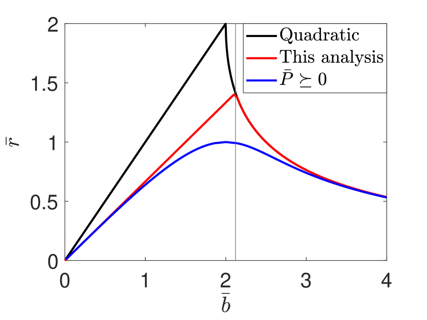
(a) Continuous setting

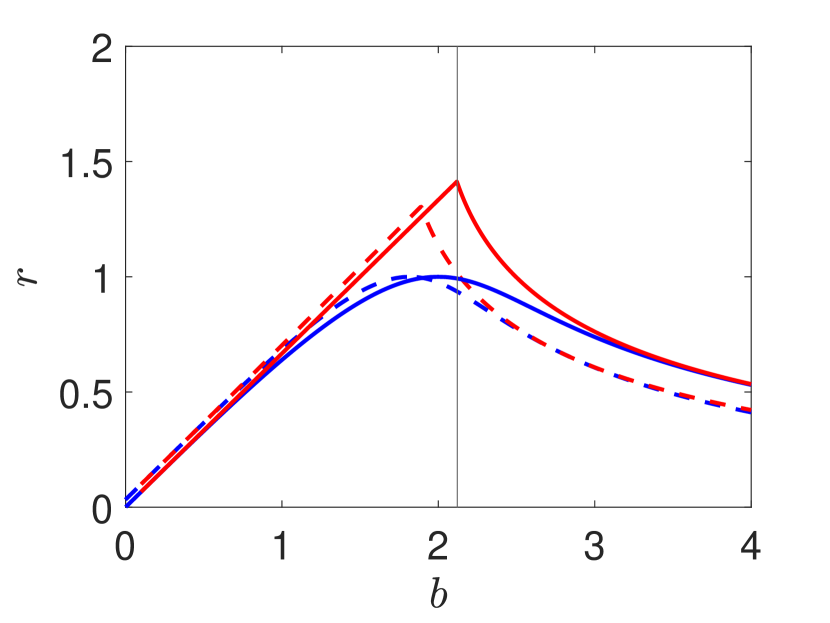
(b) Discrete setting

Figure 1: The left panel shows the relationship between the rate $\bar{r}=\lambda/\sqrt{m}$ and the parameter $\bar{b}$ in the time-continuous case. The right panel shows the relationship between the rate $r$ and the method parameter $b$ in the discrete case when $\delta=\delta_{max}=1/\sqrt{\kappa}$; the solid curves are for $\kappa=10^{6}$ and the dashed curves are for $\kappa=10^{2}$. The red curves correspond to the present analysis and the blue curves correspond to the hypothesis $\bar{P}\succeq 0$. The red and blue solid lines on the right are indistinguishable from the red and blue lines on the left.

3.1.1 A numerical illustration

We compare numerically the bound provided by the analysis just presented with the corresponding bound when operating within the framework in [27]. We use the two-dimensional objective function in $\mathcal{F}_{m,L}$ given by

$$f(x_{1},x_{2})=\frac{m}{2}(x_{1}^{2}+x_{2}^{2})+4(L-m)\log{(1+e^{-x_{1}})}$$ (3.10)

(subindices denote scalar components of the vector $x$) and for $0\leq t\leq 20$ compute solutions of (3.1) with a high-order Runge-Kutta algorithm. We report here results for $m=1$, $L=10^{6}$, when the initial condition is chosen as $x_{1}(0)=0$, $x_{2}(0)=50$, $v_{1}(0)=0$, $v_{2}(0)=0$.

The first panel in Fig. 2 corresponds to $\bar{b}=2$, the value that provides the bound with best rate when operating as in [27]. The solid straight line gives the bound (2.7) when $\bar{P}$ and $\lambda$ are taken as in the analysis in the preceding subsection; one finds $\min\sigma(\tilde{P})\approx 0.0195$, $\max\sigma(C^{\textsf{T}}C)=1$ and $\lambda=4/3$. The dashed line gives the bound (2.7) when $\bar{P}\succeq 0$ and $\lambda$ are determined as in [27]; then $\min\sigma(\tilde{P})\approx 0.1432$, $\max\sigma(C^{\textsf{T}}C)=1$ and $\lambda=1$. We see how, by relaxing the requirements on $\bar{P}$, it is possible to prove a larger rate of convergence, at the expense of increasing the factor $1/\min\sigma(\tilde{P})$ in (2.7). In this experiment, the slopes of both straight lines clearly underestimate the rate of decay in the ODE.

In the central panel of Fig. 2, $\bar{b}=2.1$, a value slightly below $3\sqrt{2}/2\approx 2.1213$. Our analysis yields $\min\sigma(\tilde{P})\approx 0.0034$, $\max\sigma(C^{\textsf{T}}C)=1$ and $\lambda=1.400$, while when working as in [27], we get $\min\sigma(\tilde{P})\approx 0.1355$, $\max\sigma(C^{\textsf{T}}C)=1$ and the quite pessimistic value $\lambda\approx 0.9950$.

In the final panel, $b=2.2>3\sqrt{2}/2$. Now our analysis has $\min\sigma(\tilde{P})\approx 0.0319$, $\max\sigma(C^{\textsf{T}}C)=1$ and $\lambda=1.2835$, and, under the hypotheses of [27], $\min\sigma(\tilde{P})\approx 0.1493$, $\max\sigma(C^{\textsf{T}}C)=1$ and $\lambda\approx 0.9807$. The slope of the the continuous line describes very well the decay behaviour of the ODE (note that, for this value of $\bar{b}$, the rate proved here cannot be improved, as it coincides with the rate the ODE achieves on linear problems). As it is the case for the other two values of $\bar{b}$, the rate that may be proved under the assumption $\bar{P}\succeq 0$ is unduly pessimistic.

By comparing the three panels, we see that the value of the friction parameter that leads to a faster decay of the ODE solution is $\bar{b}=2$, i.e. the best choice for quadratic objective functions. In this regard, we note that once $t$ is so large that $x(t)$ is close to $x^{\star}$, the objective function becomes approximately quadratic $f(x)\approx f(x^{\star})+(1/2)(x-x^{\star})^{\textsf{T}}H(x-x^{\star})$, with $H$ given by the Hessian matrix of $f$ evaluated at the minimizer.

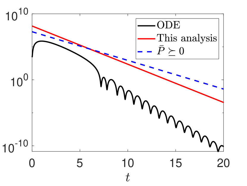
(a) $\bar{b}=2$

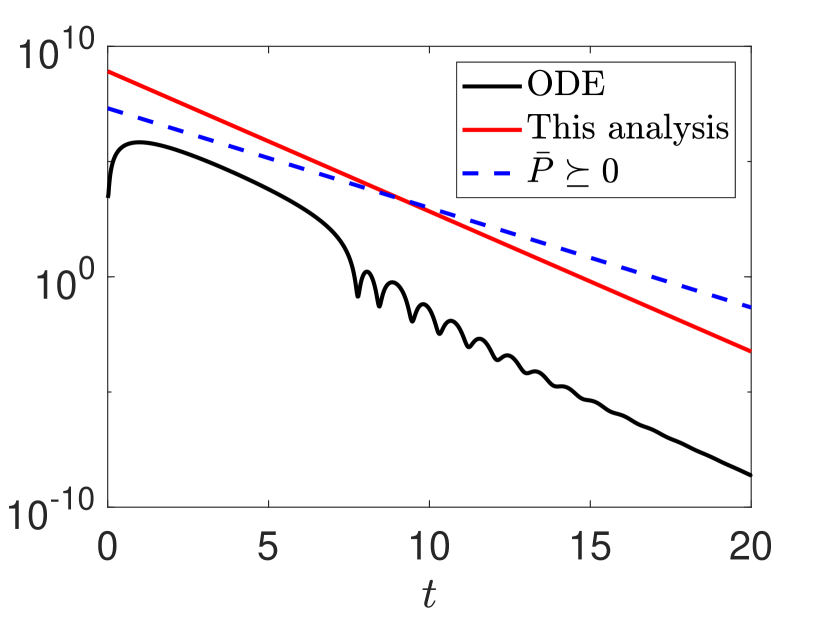
(b) $\bar{b}=2.1$

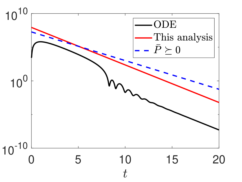
(c) $\bar{b}=2.2$

Figure 2: Polyak ODE. Bounds for $\lVert x(t)-x^{\star}\rVert^{2}$ for different values of the parameter $\bar{b}$, when $f$ is given by (3.10), $m=1$, $L=10^{6}$ .

3.2 Discrete time analysis

We will now study optimization methods of the form (1.3) for $\alpha_{k}=\alpha$ and $\beta_{k}=\beta$. In order to easily relate what follows to the time-continuous case, we first introduce as a new variable the divided difference, $k=1,2,\dots$,

$$d_{k}=\frac{1}{\delta}(x_{k}-x_{k-1}),$$

where the steplength $\delta=\sqrt{m\alpha}$ is nondimensional ($\beta$ is also nondimensional). With the new variable, (1.3) becomes ($k=0,1,\dots$)

$$d_{k+1} =\beta d_{k}-\frac{\alpha}{\delta}\nabla f(y_{k}),$$ (3.11a)

$$x_{k+1} =x_{k}+\delta\beta d_{k}-\alpha\nabla f(y_{k}),$$ (3.11b)

$$y_{k} =x_{k}+\delta\beta d_{k},$$ (3.11c)

and these equations are of the form (2.2) with $\xi_{k}=[d_{k}^{\textsf{T}},x_{k}^{\textsf{T}}]^{\textsf{T}}\in\mathbb{R}^{2d}$ and

$$A=\left[\begin{matrix}\beta I_{d}&0\\ \delta\beta I_{d}&I_{d}\end{matrix}\right],\quad B=\left[\begin{matrix}-(\alpha/\delta)I_{d}\\ -\alpha I_{d}\end{matrix}\right],\quad C=\left[\begin{matrix}\delta\beta I_{d}&I_{d}\end{matrix}\right],\quad E=\left[\begin{matrix}0&I_{d}\end{matrix}\right].$$

According to Theorem 2.3, in order to identify a convergence rate for (1.3), it is sufficient to find numbers $a_{0}>0$, $\rho\in(0,1)$, $\ell\geq 0$ and a matrix $P$ with $P+(a_{0}m/2)E^{\textsf{T}}E\succ 0$ such that $T$ in (2.9) is $\preceq 0$. Similarly to the previous subsection, we set $\ell=0$, as this does not have a significant impact on the value of $\rho$ that results from the analysis. This, in turn, allows us to further simplify things, since $T$ is homogeneous in $P$ and $a_{0}$ and we may assume $a_{0}=1$. Then $T$ is a function of $P$ and $\rho$ (and the method parameters $\beta$ and $\delta$).

Similarly to the continuous case, the Kronecker product structure of the matrices $A,B,C,E$ leads us to look for a $2\times 2\ \widehat{P}$ and a $3\times 3\ \widehat{T}$ as in equations (3.3) and (3.4), rather than for $P$ and $T$. The elements of $\widehat{T}$ are found to be

$$t_{11} =\beta^{2}p_{11}+2\delta\beta^{2}p_{12}+\delta^{2}\beta^{2}p_{22}-\rho^{2}p_{11}-\delta^{2}\beta^{2}m/2,$$

$$t_{12} =\beta p_{12}+\delta\beta p_{22}-\rho^{2}p_{12}-\delta\beta m/2+\rho^{2}\delta\beta m/2,$$

$$t_{13} =-\delta^{-1}\alpha\beta p_{11}-2\alpha\beta p_{12}-\delta\alpha\beta p_{22}+\delta\beta/2,$$

$$t_{22} =p_{22}-\rho^{2}p_{22}-m/2+\rho^{2}m/2,$$

$$t_{23} =-\delta^{-1}\alpha p_{12}-\alpha p_{22}+1/2-\rho^{2}/2,$$

$$t_{33} =\delta^{-2}\alpha^{2}p_{11}+2\delta^{-1}\alpha^{2}p_{12}+\alpha^{2}p_{22}+\alpha^{2}L/2-\alpha.$$

Note that in the limit $\alpha\to 0$, these elements converge to those of the continuous case.

Our objective is to find $\rho\in(0,1)$, $p_{11}$, $p_{12}$, and $p_{22}$ that lead to $\widehat{T}\preceq 0$ and $\widehat{P}+(m/2)\widehat{E}^{\textsf{T}}\widehat{E}\succ 0$ (which in turn imply $T\preceq 0$ and $P+(m/2)E^{\textsf{T}}E\succ 0$). The algebra becomes simpler if we represent $\beta$ and $\rho^{2}$ as

$$\beta=1-b\delta,\qquad\rho^{2}=1-r\delta.$$

In the continuous case (first and second steps), we had $\bar{t}_{13}=0$ and $\bar{t}_{23}=0$, and we now similarly impose the conditions ${t}_{13}=0$ and ${t}_{23}=0$, which leads to

$$p_{11} =p_{22}\delta^{2}-mr\delta+\frac{m}{2},$$

$$p_{12} =\frac{mr}{2}-\delta p_{22}.$$

These relations imply

$$t_{33}=\frac{1}{2}\alpha(L\alpha-1),$$

so that we require $\alpha\leq 1/L$ in order to guarantee $t_{33}\leq 0$. In other words, the step length has to satisfy $\delta\leq\delta_{\max}=1/\sqrt{\kappa}$.

Having dealt with the third row/column of $\widehat{T}$, we have to take care of the submatrix consisting of the first and second rows/columns. If $\Delta$ denotes the determinant of that submatrix, we need $\Delta\geq 0$. As in the third step of the continuous case, we impose the conditions $\Delta=0$ and $(\partial/\partial p_{22})\Delta=0$. The second of these relations yields

$$p_{22}=mr\frac{b^{2}\delta^{3}-b^{2}\delta-2rb\delta^{3}+2rb\delta+3r\delta^{2}-2\delta-r}{(4\delta r-4)},$$

an expression that reduces to (3.8) for $\delta=0$. Similar to the continuous case, the expression for $p_{22}$ is substituted in the equation $\Delta=0$. This gives a relation $\varphi(r,b;\delta)=0$ between the method parameter $b$ and the rate $r$ for each choice of $\delta$. Unlike the simpler continuous case, where the function $r=r(\bar{b})$ was found analytically, we have to proceed numerically and for given $\delta$, we solve numerically for $r$ on a grid of values of $b$, while at the same time checking the conditions $P+(m/2)E^{\textsf{T}}E\succ 0$ and $t_{22}\leq 0$ (the latter guarantees $T\preceq 0$).

For two values of $\delta_{max}$, we plot in Figure 1(b) the curve $\Delta=0$ for the most favourable step length $\delta=\delta_{max}$ and, in addition, we compare with the analogous curve obtained in [27] under the constraint $P\succeq 0$ required by the framework in [7]. In [27] the best achievable rate is $r=1$. As we may see, by changing the constraint on $P$ it is possible to prove a significantly better convergence rate. In particular, for the modified constraint in the present analysis, one can show easily that $b$ may be chosen to get $r=\sqrt{2}-\mathcal{O}(\delta)$, which in turn implies that for $\delta=\delta_{max}$ in (2.10):

$$\rho^{2}=1-\frac{\sqrt{2}}{\sqrt{\kappa}}+\mathcal{O}\left(\frac{1}{\kappa}\right),\quad\kappa\rightarrow\infty.$$

Remark 3.2.

The parameter values $\alpha=1/L$ and $\beta=(1-\sqrt{m\alpha})/(1-\sqrt{m\alpha})$ in (1.3) (the standard choice for Nesterov algorithm) lead to the best convergence rate that may be established with the approach in [27]. The present analysis shows that higher convergence rates may be rigorously proved for larger values of $\beta$ as illustrated in Figure 1(b).

4 Connecting optimization algorithms and Polyak’s ODE

We now discuss the relations between the continuous and discrete time studies presented above.

4.1 The Nesterov algorithm as an integrator

For suitable parameter choices, the Nesterov algorithm (1.3) is a discretization of Polyak differential equation. However, as discussed in detail in [27], such a discretization does not correspond to any of the more familiar classes of ODE solvers, such as linear multistep or Runge Kutta (RK) methods. In particular we remark that in (1.3) $\nabla f$ is not evaluated at the approximations $x_{k}$ delivered by the algorithm. As we shall see presently, it turns out that the Nesterov algorithm is an example of the class of Additive Runge-Kutta (ARK) algorithms, a generalization of the RK integrators considered by several authors after its introduction by Cooper [3, 4].

Additive Runge-Kutta (ARK) algorithms integrate systems of differential equations $(d/dt)z=g(z)$ in cases where it makes sense to decompose $g(z)$ as a sum $g(z)=\sum_{\nu=1}^{N}g^{[\nu]}(z)$. In the plain RK case, the numerical solution is advanced over a time step $z_{k}\mapsto z_{k+1}$ by evaluating $g(z)$ at a sequence of so-called stage vectors $Z_{k,1}$, …, $Z_{k,s}$ and then setting $z_{k+1}=z_{k}+\sum_{i=1}^{s}b_{i}g(Z_{k,i})$, where the $b_{i}$ are suitable weights. In turn, for the explicit algorithms we are interested in, the stages are computed successively, $i=1,\dots,s$, as $Z_{k,i}=z_{k}+h\sum_{j=1}^{i-1}a_{i,j}g(Z_{k,j})$, with suitable coefficients $a_{i,j}$. ARK algorithms are entirely similar, but evaluate the individual pieces $g^{[\nu]}(z)$ rather than $g(z)$.

With $z=[v^{\textsf{T}},x^{\textsf{T}}]^{\textsf{T}}\in\mathbb{R}^{2d}$, the system (3.1) may be rewritten as

$$\frac{d}{dt}z=g^{[1]}(z)+g^{[2]}(z)+g^{[3]}(z):=\begin{bmatrix}-\bar{b}\sqrt{m}v\\ 0\end{bmatrix}+\begin{bmatrix}-\frac{1}{\sqrt{m}}\nabla f(x)\\ 0\end{bmatrix}+\begin{bmatrix}0\\ \sqrt{m}v\end{bmatrix};$$

the three parts of $g(z)$ respectively represent the friction force, potential force and inertia in the oscillator. It is easily checked that, if we choose a steplength $h>0$, and see $d_{k}$ and $x_{k}$ as approximations to $v(kh)$ and $x(kh)$ respectively, then a step $(d_{k},x_{k})\mapsto(d_{k+1},x_{k+1})$ of the optimization algorithm (3.11) with parameters $\alpha=h^{2}$, $\beta=1-h\bar{b}\sqrt{m}$, $\delta=\sqrt{m}h$ is just one step $z_{k}\mapsto z_{k+1}$ of the ARK integrator for (3.1) given by:

$$Z_{k,1} = z_{k},$$

$$Z_{k,2} = z_{k}+hg^{[1]}(Z_{k,1}),$$

$$Z_{k,3} = z_{k}+hg^{[1]}(Z_{k,1})+hg^{[3]}(Z_{k,2}),$$

$$Z_{k,4} = z_{k}+hg^{[1]}(Z_{k,1})+hg^{[3]}(Z_{k,2})+hg^{[2]}(Z_{k,3}),$$

$$z_{k+1} = z_{k}+hg^{[1]}(Z_{k,1})+hg^{[2]}(Z_{k,3})+hg^{[3]}(Z_{k,4}).$$

The stage vectors have $Z_{k,1}=[d_{k}^{\textsf{T}},x_{k}^{\textsf{T}}]^{\textsf{T}}$, $Z_{k,2}=[\beta d_{k}^{\textsf{T}},x_{k}^{\textsf{T}}]^{\textsf{T}}$, $Z_{k,3}=[\beta d_{k}^{\textsf{T}},y_{k}^{\textsf{T}}]^{\textsf{T}}$, $Z_{k,4}=[d_{k+1}^{\textsf{T}},y_{k}^{\textsf{T}}]^{\textsf{T}}$, and therefore the computation of the second, third and fourth stages incorporate successively the contributions of friction, inertia and potential force.

If we now think that the value of $h>0$ varies and consider the optimization algorithm (3.11) with $\alpha=h^{2}$, $\beta=1-h\bar{b}\sqrt{m}$, the standard theory of numerical integration of ODEs shows that, if the initial points $x_{-1}$ and $x_{0}$ are chosen in such a way that, as $h\rightarrow 0$, $x_{0}$ and $(1/h)(x_{0}-x_{-1})$ converge to limits $A$ and $B$, then, in the limit of $kh\rightarrow t$, $x_{k}$ and $(1/h)(x_{k+1}-x_{k})$ converge to $x(t)$ and $\dot{x}(t)$ respectively, where $x(t)$ is the solution of (1.4) with initial conditions $x(0)=A$ and $\dot{x}(0)=B$. In addition, the discrete Lyapunov function of the optimization algorithm in Section 3 may be shown to converge to the Lyapunov function of the ODE found in this section. Finally the discrete decay factor over $k$ steps $(1-\sqrt{m}rh)^{k}$ converges to the continuous decay factor $\exp(-\lambda t)$. These facts in particular explain that, in Figure 1, the graph of the relation between $\bar{b}$ and $\bar{r}$ that holds for the ODE is indistinguishable from the corresponding graph for the optimization algorithm when $\kappa$ is large ($\kappa$ being large corresponds to $h$ being small).

4.2 Discretizations that do not succeed in getting acceleration

Many recent contributions have derived optimization algorithms by discretizing suitably chosen dissipative ODEs. It is well known that, unfortunately, many properties of ODEs are likely to be lost in the discretization process, even if high-order, sophisticated integrators are used. The archetypical example is provided by the discretization of the standard harmonic oscillator: most numerical methods, regardless of their accuracy, provide solutions that either decay to the origin or spiral out to infinity as the number of computed points grows unboundedly. Similarly, discretizations of (1.4) are likely not to share the favourable decay properties in Section 3.1.

Let us consider the following extension of the optimization algorithm (1.3):

$$x_{k+1} =y_{k}+\beta(x_{k}-x_{k-1})-\alpha\nabla f(y_{k}),$$ (4.1a)

$$y_{k} =x_{k}+\gamma(x_{k}-x_{k-1}),$$ (4.1b)

with the additional parameter $\gamma$. The choice $\gamma=0$ yields the heavy ball algorithm, which (see [27]) corresponds to a “natural” standard linear multistep discretization of the Polyak equation (1.4) where $\nabla f$ is evaluated at the approximations $x_{k}$. Unfortunately the heavy ball algorithm does not provide acceleration. As shown in [27] for $\gamma=0$ (or more generally for $\gamma\neq\beta$), the optimization algorithm (4.1) does not inherit a Lyapunov functions from the Polyak ODE. The analysis in that paper hinges on a study of the nondimensional quantity $c:=t_{11}/(m\delta)$, which for $\widehat{T}\preceq 0$ has to be $\leq 0$ and for a discretization of an ODE has a finite limit as $\delta\rightarrow 0$. When $\gamma=0$, the expression for the quantity $c$ includes a positive contribution $\delta(\kappa-1)\beta^{2}/2$; for acceleration, $\delta$ has to be $\mathcal{O}(1/\sqrt{\kappa})$ which makes it impossible for $c$ to be $\leq 0$.

The unwelcome presence of $\kappa$ in $t_{11}$ may be traced back to the appearance of $L$ in the matrix $N^{(1)}$ in Theorem 2.3. Nesterov’s algorithms of the family (1.3) do not suffer from that appearance because for them the matrix $EA-C$ that multiplies $(L/2)I_{d}$ in the recipe for $N^{(1)}$ vanishes. The condition $EA-C=0$ appears then to be of key importance in the success of Nesterov algorithms; we put it into words by saying that one has to impose that the point $y_{k}=C\xi_{k}$ where the gradient is evaluated has to coincide with the point $x_{k+1}=EA\xi_{k}$ that the algorithm would yield if $u_{k}=\nabla f(y_{k})$ happened to vanish (see (2.2)). This suggests that the integrator has to treat the potential force and the friction force in the oscillator separately, something that may be achieved by ARK algorithms but not by more conventional linear multistep or RK methods that do not avail themselves of the separate pieces $g^{[1]}(z)$, $g^{[2]}(z)$, $g^{[3]}(z)$ but are rather formulated in terms of $g(z)$.

5 Derivation and analysis of a new second order ODE

In the last few years there has been a number of works that have studied ways of accelerating convergence towards equilibrium for dynamics of stochastic differential equations [15, 5, 9, 11, 12] . When the dynamics of the underlying SDE are linear this problem is directly connected to finding the minimum of a quadratic function $f(x)=(1/2)x^{\textsf{T}}Sx+c^{\textsf{T}}x$, with $S=S^{\textsf{T}}\succ 0$. For simplicity we will assume that $c=0$ and in this case the GF (1.2) obtains the simple form

$$\frac{dx}{dt}=-Sx$$

and the speed of convergence towards zero is dictated by the minimum eigenvalue of $S$. It is possible to increase the speed of convergence towards zero by introducing a non-reversible perturbation to the above equation. More precisely, it is easy to show [15] that the dynamics of

$$\frac{dx}{dt}=-(I+J)Sx,\qquad J=-J^{\textsf{T}}$$

yields faster convergence towards zero than the original GF. Furthermore, as discussed in [15] there is an optimal perturbation $J^{\star}$ for which the rate of convergence towards zero is maximized, with the maximum value being $\text{Tr}(S)/d$ where $d$ is the dimension of the matrix. A natural question to ask is if this kind of acceleration remains true when $f\in\mathcal{F}_{m,L}$ is not quadratic. In this case the perturbed ODE has the form

$$\frac{dx}{dt}=-(I+J)\nabla f(x),\quad J=-J^{\textsf{T}}.$$

This equation and discretizations of it were studied in [10]. In particular, it was shown that upon assuming additional information about the eigenvalues of the Hessian of $f$, convergence rates may improve both in the continuous and discrete setting. Here we will instead consider the GD (1.2) for an appropriately chosen extended objective function and modify its dynamics with a simple non-reversible perturbation. In this case it is possible to fully quantify the increase in the convergence rate without any additional assumptions on $f$.

We introduce an auxiliary variable $y\in\mathbb{R}^{d}$ and the extended objective function $F(y,x)=(L/2)\lVert y\rVert^{2}+f(x)$ with minimum at $(0,x^{\star})$. The corresponding GF is

$$\frac{d}{d\tau}\left[\begin{matrix}y\\ x\end{matrix}\right]=-\left[\begin{matrix}Ly\\ \nabla f(x)\end{matrix}\right]$$

and we perturb the right hand-side by adding a skew-symmetric term to get

$$\frac{d}{d\tau}\left[\begin{matrix}y\\ x\end{matrix}\right]=-\left[\begin{matrix}Ly\\ \nabla f(x)\end{matrix}\right]+K\left[\begin{matrix}0&-I\\ I&0\end{matrix}\right]\left[\begin{matrix}Ly\\ \nabla f(x)\end{matrix}\right]$$

where $K\geq 0$ is a perturbation parameter. For $K=0$, $x$ evolves as in (1.2) (but the time variable here has been relabelled for reasons that will become clear immediately). By replacing the variables $y$ and $\tau$ and the parameter $K$ by $v$, $t$ and $\bar{b}\geq 0$ respectively, with

$$y=\sqrt{\frac{m}{L}}v,\qquad\tau=\frac{\bar{b}\sqrt{m}}{L}t,\qquad K=\frac{1}{\bar{b}}\sqrt{\frac{L}{m}},$$

the system becomes

$$\frac{d}{dt}v =-\bar{b}\sqrt{m}v-\frac{1}{\sqrt{m}}\nabla f(x),$$ (5.1a)

$$\frac{d}{dt}x =\frac{\bar{b}\sqrt{m}}{L}\nabla f(x)+\sqrt{m}v.$$ (5.1b)

Comparing these expressions with (3.1), we see that we are dealing here with a perturbation of Polyak’s equation, where now $\nabla f(x)$ is used both in the $v$ and $x$ equations; Polyak equation is retrieved in the limit $L\uparrow\infty$ with fixed $m$. For this reason we shall refer to (5.1) as the Polyak+ system. As noted before, as the friction coefficient $\bar{b}$ grows unboundedly (i.e. $K\downarrow 0$) with fixed $L$ and $m$, the dynamics of $x$ under (5.1) approaches GD; on the other hand, in the limit $\bar{b}\downarrow 0$, (5.1) becomes a Hamiltonian (nondissipative) system.

The system (5.1) is easily cast in the control framework of Section 2 and we use Theorem 2.1 to investigate to what extent it improves on Polyak’s ODE. The $\bar{t}_{ij}$ in (3.4) are found to be

$$\bar{t}_{11} =-2\bar{b}\sqrt{m}\bar{p}_{11}+2\sqrt{m}\bar{p}_{12}+\lambda\bar{p}_{11},$$

$$\bar{t}_{12} =-\bar{b}\sqrt{m}\bar{p}_{12}+\sqrt{m}\bar{p}_{22}+\lambda\bar{p}_{12},$$

$$\bar{t}_{13} =-(1/\sqrt{m})\bar{p}_{11}+\sqrt{m}/2-\bar{b}\sqrt{m}\bar{p}_{12}/L,$$

$$\bar{t}_{22} =\lambda\bar{p}_{22}-(m/2)\lambda,$$

$$\bar{t}_{23} =-(1/\sqrt{m})\bar{p}_{12}+\lambda/2-\bar{b}\sqrt{m}\bar{p}_{22}/L,$$

$$\bar{t}_{33} =-\bar{b}\sqrt{m}/L.$$

To carry out the analysis it is convenient to introduce $\zeta=1/L$; the limit value $\zeta=0$ then corresponds to Polyak’s ODE. We saw in Section 3.1 that, in the $\zeta=0$ case, each rate $\bar{r}<\sqrt{2}$ may be achieved with two different values of $\bar{b}$, one below $3\sqrt{2}/2$ and the other above. We have carried out the analysis of (5.1) for $\bar{b}<3\sqrt{2}/2$. When determining $\lambda=\sqrt{m}\bar{r}$ and the elements $\bar{p}_{ij}$ we operate under the following two assumptions:

1. The matrix $\widehat{\bar{T}}$ has rank $\leq 1$.

2. We have

   $$\bar{p}_{11}=m/2.$$ (5.2)

In extensive experimentation we have observed that these two conditions hold when $\lambda$ is numerically maximized subject to the constraints $\widetilde{P}\succ 0$, $\widehat{\bar{T}}\preceq 0$. Note also that they are satisfied in Polyak’s, $\zeta=0$, case: for the first assumption recall that we saw in Section 3.1 that, for $\bar{b}<3\sqrt{2}/2$ , when $\bar{r}$ is maximized all elements of $\widehat{\bar{T}}$ vanish, except perhaps $\bar{t}_{22}$ and for the second assumption see (3.5). We point out that Assumption 1 is equivalent to the requirement that all $2\times 2$ submatrices of $\widehat{\bar{T}}$ are singular.

The assumptions above uniquely determine $\lambda$ and $\bar{P}$ in Theorem 2.1. We proceed as follows:

• By imposing that the determinant of the first and third rows and columns of $\widehat{\bar{T}}$ vanish we find

  $$\bar{r}=2\bar{b}-(4/m)\bar{p}_{12}-(2\bar{b}/m)\bar{p}_{12}^{2}\zeta.$$ (5.3)

• By annihilating the determinant of the second and third rows and first and third columns

  $$\bar{p}_{22}=\bar{p}_{12}^{2}/m.$$ (5.4)

• We take the expressions for $\bar{r}$ and $\bar{p}_{22}$ just found to the equation $\bar{t}_{22}\bar{t}_{33}-\bar{t}_{23}^{2}=0$. This yields an algebraic relation between $\bar{p}_{12}$ and $\zeta$:

  $$(2\bar{b}^{2}\bar{p}_{12}^{4}+m^{2}\bar{b}^{2}\bar{p}_{12}^{2})\zeta^{2}+(8\bar{b}\bar{p}_{12}^{3}-2m\bar{b}^{2}\bar{p}_{12}^{2}+2m^{2}\bar{b}\bar{p}_{12}-m^{3}\bar{b}^{2})\zeta+(-3\bar{p}_{12}+m\bar{b})^{2}=0.$$ (5.5)

The conditions (5.3)–(5.5) guarantee that the rank of $\widehat{\bar{T}}$ is $\leq 1$, i.e. the matrix has at least two zero eigenvalues. Since $\bar{t}_{33}<0$ for $\bar{b}>0$ and $\zeta>0$ the matrix will have rank exactly one and be negative semidefinite.

The algebraic curve (5.5) in the $(\bar{p}_{12},\zeta)$ plane contains the points $P_{1}=(0,1/m)$ and $P_{2}=(m\bar{b}/3,0)$. The first corresponds to the $L=m$ (i.e. $\kappa=1$) situation; the second was known to us at it corresponds to Polyak’s equation. The global behavior of the curve (5.5) may be investigated by solving the quadratic equation for $\zeta$. Restricting the attention to $0\leq\bar{p}_{12}\leq m\bar{b}/3$, there is a branch of the curve where to each value of $\bar{p}_{12}$ there corresponds a unique value of $\zeta$ (i.e. of $L$), so that as $\bar{p}_{12}$ increases monotonically from $0$ to $m\bar{b}/3$, $\zeta$ decreases monotonically from $1/m$ to $0$ (or $\kappa$ increases from $1$ to $\infty$). Note that this branch connects the points $P_{1}$ and $P_{2}$. Once $\zeta=\zeta(\bar{p}_{12})$, for given $m$, $\bar{b}$, has been determined in this way, the relations (5.2)–(5.4) determine $\bar{r}$, $\bar{p}_{11}$, $\bar{p}_{22}$ as functions of $\bar{p}_{12}\in[0,m\bar{b}/3]$ with known expressions (that we will not reproduce here). It is easily checked that, for the values of $\bar{p}_{ij}$ defined in this way, $\widetilde{P}$ is in fact $\succ 0$. Numerical experiments confirm that maximizing $\lambda$ subject to the constraints $\widetilde{P}\succ 0$, $\widehat{\bar{T}}\preceq 0$ for different choices of $L$, $m$ and $\bar{b}$ leads to the values of $\bar{p}_{ij}$ and $\bar{r}$ we have just constructed analytically. This confirms that the procedure we have followed succeeds in identifying the best $\lambda$ and $\bar{P}$ in Theorem 2.1 or, in other words, that the assumptions 1-2 formulated at the outset are valid.

In Fig. 3 we have plotted in the $(\kappa,\bar{r})$ plane the parametric curve $\kappa=L/m=1/(m\zeta(\bar{p}_{12}))$, $\bar{r}=\bar{r}(p_{12})$, $\bar{p}_{12}\in[0,m\bar{b}/3]$ when $\bar{b}=2$. Although the system (5.1) clearly improves on Polyak’s dynamics for small $\kappa$, the improvement becomes negligible as $\kappa$ increases, i.e. in the regime where it would really be needed. We now make this matter more precise.

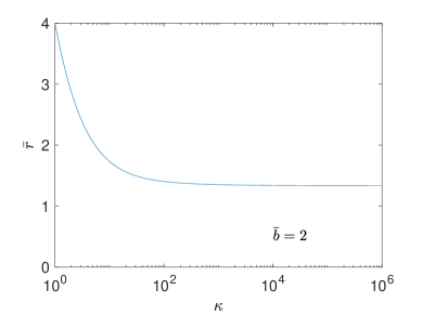
Figure 3: Converge rate $r$ as a function of the condition number $\kappa$ for (5.1)

At the point $P_{1}$, where $\kappa=1$, (5.3) yields $\bar{r}=2\bar{b}$; this is to be compared with the value $\bar{r}=2\bar{b}/3$ obtained in Section 3 for Polyak’s equation. The introduction of gradient in the first equation in (5.1) increases $\lambda$ by a factor of $3$.

Let us now consider the neighbourhood of the point $P_{2}$, i.e. the $\kappa\gg 1$ regime. By implicit differentiation of (5.5), we find that, at this point, the Taylor expansion of $\zeta$ as a function of $p_{12}$ is given by

$$\zeta=\frac{243}{9\bar{b}^{2}-2\bar{b}^{4}}\big{(}p_{12}-\frac{\bar{b}}{3}\big{)}^{2}+\mathcal{O}\Big{(}\big{(}p_{12}-\frac{\bar{b}}{3}\big{)}^{3}\Big{)},\qquad\bar{p}_{12}\rightarrow m\bar{b}/3.$$

On the other hand, using the expression of $\bar{r}$ as a function of $\bar{p}_{12}$, one finds

$$\bar{r}=\frac{2\bar{b}}{3}-\frac{4}{m}\left(\bar{p}_{12}-\frac{m\bar{b}}{3}\right)+\mathcal{O}\left(\bar{p}_{12}-\frac{m\bar{b}}{3}\right)^{2},\qquad\bar{p}_{12}\rightarrow m\bar{b}/3$$

and, combining the last equations, we obtain after eliminating $\bar{p}_{12}$,

$$\bar{r}=\frac{2\bar{b}}{3}+C(\bar{b})\frac{1}{\sqrt{\kappa}}+\mathcal{O}\left(\frac{1}{\kappa}\right),\qquad\kappa\rightarrow\infty,$$ (5.6)

with

$$C(\bar{b})=4\sqrt{\frac{9\bar{b}^{2}-2\bar{b}^{4}}{243}},\qquad\bar{b}<3\sqrt{2}/2.$$

Since $C(\bar{b})>0$, we conclude that, for large condition number $\kappa$, the Polyak+ system in fact achieves a rate larger than the rate ${2\bar{b}}/{3}$ for Polyak’s ODE. Unfortunately, in order to maximize the leading term, $2\bar{b}/3$, in the expansion (5.6), $\bar{b}$ has to be chosen close to the upper limit $3\sqrt{2}/2$ and, as $\bar{b}\uparrow 3\sqrt{2}/2$, the increment $C(\bar{b})/\sqrt{\kappa}$ vanishes. For instance, for $\bar{b}=2.1$, (5.6) becomes $\bar{r}\approx 1.4000+0.2286/\sqrt{\kappa}$; for $\kappa=10^{4}$ the increment is only 0.0022. Therefore, as in the particular case depicted in Fig. 3, the improvement in rate of the Polyak+ system on the Polyak ODE is indeed negligible, except in the uninteresting case of small $\kappa$. For this reason we have not undertaken the analysis of optimization algorithms based on discretizations of the Polyak+ system.

6 Stochastic problems: The case of over-parameterized models

In this section, we extend the Lyapunov function approach to analyse the performance of optimization methods applied to specific modern machine learning models. In particular, we study models such as non-parametric regression or overparameterised deep neural models that are expressive enough to fit or interpolate the data set completely [34, 17]. For these models the function $f(x)$ that one is interested in minimising has the following structure

$$f(x)=\frac{1}{N}\sum_{i=1}^{N}f_{i}(x).$$ (6.1)

Due to the structure of $f$ in (6.1) any gradient based algorithm would need to calculate

$$\nabla f(x)=\frac{1}{N}\sum_{i=1}^{N}\nabla f_{i}(x)$$

which when $N$ is large may be computationally very expensive. A typical strategy followed in stochastic optimization algorithms is to replace the gradient with a random unbiased estimator of it. In the simplest possible case, one uses the following estimator

$$\widehat{\nabla}f(x)=\nabla f_{i_{\omega}}$$

where $i_{\omega}$ is a uniform random variable in the set of integers $\{1,\cdots,n\}$. More generally, and without necessarily assuming the finite sum-structure one replaces the full gradient by

$$\widehat{\nabla}f(x)=\nabla f(x,z)$$

where $z$ can be thought of as the random gradient noise, which we assume satisfies $\mathbb{E}(\nabla f(x,z))=\nabla f(x)$.

6.1 A framework for stochastic algorithms

We consider optimization algorithms with random noise analogously to (2.2) with the formulation

$$\xi_{k+1} =A\xi_{k}+B\tilde{u}_{k},$$ (6.2a)

$$\tilde{u}_{k} =\widehat{\nabla}f(y_{k}),$$ (6.2b)

$$y_{k} =C\xi_{k},$$ (6.2c)

$$x_{k} =E\xi_{k},$$ (6.2d)

where $\xi_{k}\in\mathbb{R}^{n}$ is the state, $\tilde{u}_{k}\in\mathbb{R}^{d}$ is the random input $(d\leq n)$, $y_{k}\in\mathbb{R}^{d}$ is the feedback output that is mapped to $\tilde{u}_{k}$ by the random nonlinear map $\widehat{\nabla}f$. We assume here that at each step the random gradient is chosen to be independent of the current state, i.e. $\widehat{\nabla}f(y_{k})=\nabla f(y_{k},z_{k})$ for some random variable $z_{k}$ independent of $y_{k}$.

Theorem 6.1.

Suppose that, for (6.2), there exist $a_{0}>0$, $\rho\in(0,1)$, and a symmetric matrix $P$, with $\widetilde{P}:=P+(a_{0}m/2)E^{\textsf{T}}E\succ 0$, such that

$$T=M^{(0)}+a_{0}\rho^{2}M^{(1)}+a_{0}(1-\rho^{2})M^{(2)}\preceq 0,$$ (6.3)

where

$$M^{(0)}=\left[\begin{matrix}A^{\textsf{T}}PA-\rho^{2}P&A^{\textsf{T}}PB\\ B^{\textsf{T}}PA&\rho_{0}B^{\textsf{T}}PB\end{matrix}\right],$$

and

$$M^{(1)}=N^{(1)}+N^{(2)},\quad M^{(2)}=N^{(1)}+N^{(3)},$$

with

$$N^{(1)} =\left[\begin{matrix}\frac{L}{2}(EA-C)^{\textsf{T}}(EA-C)&\frac{1}{2}(EA-C)^{\textsf{T}}(LEB+1)\\ \frac{1}{2}(LEB+1)^{\textsf{T}}(EA-C)&\frac{L\rho_{0}}{2}(EB)^{\textsf{T}}EB+\frac{1}{2}(EB+(EB)^{\textsf{T}})\end{matrix}\right],$$

$$N^{(2)} =\left[\begin{matrix}C-E&0\\ 0&I_{d}\end{matrix}\right]^{\textsf{T}}\left[\begin{matrix}-\frac{m}{2}I_{d}&\frac{1}{2}I_{d}\\ \frac{1}{2}I_{d}&0\end{matrix}\right]\left[\begin{matrix}C-E&0\\ 0&I_{d}\end{matrix}\right],$$

$$N^{(3)} =\left[\begin{matrix}C^{\textsf{T}}&0\\ 0&I_{d}\end{matrix}\right]\left[\begin{matrix}-\frac{m}{2}I_{d}&\frac{1}{2}I_{d}\\ \frac{1}{2}I_{d}&0\end{matrix}\right]\left[\begin{matrix}C&0\\ 0&I_{d}\end{matrix}\right].$$

Assume there exists $\rho_{0}>0$ such that for all $y\in\mathbb{R}^{d}$

$$\mathbb{E}[\widehat{\nabla}f(y)^{\textsf{T}}(EB)^{\textsf{T}}(EB)\widehat{\nabla}f(y)]\leq\rho_{0}\nabla f(y)^{\textsf{T}}(EB)^{\textsf{T}}(EB)\nabla f(y),$$ (6.4a)

$$\mathbb{E}[\widehat{\nabla}f(y)^{\textsf{T}}B^{\textsf{T}}PB\widehat{\nabla}f(y)]\leq\rho_{0}\nabla f(y)^{\textsf{T}}B^{\textsf{T}}PB\nabla f(y).$$ (6.4b)

Then, for $f\in\mathcal{F}_{m,L}$, $\rho_{0}>1$ and $V$ given by (2.8), the sequence $\{x_{k}\}$ satisfies

$$\mathbb{E}[\lVert x_{k}-x^{\star}\rVert^{2}]\leq\max\sigma(E^{\textsf{T}}E)\mathbb{E}[\lVert\xi_{k}-\xi^{\star}\rVert]\leq\frac{\max\sigma(E^{\textsf{T}}E)}{\min\sigma(\widetilde{P})}V_{0}(\xi_{0})\rho^{2k}.$$

Proof.

The proof of this theorem follows the same argument as the proof of Theorem 2.3 except for the derivation of $N^{(1)}$ and $M^{(0)}$; therefore we only show how these terms differ. Using the Equation (6.2) we have

$$\left[\begin{matrix}x_{k+1}-y_{k}\\ \nabla f(y_{k})\end{matrix}\right]=\left[\begin{matrix}EA-C&EB&0\\ 0&0&I_{d}\end{matrix}\right]\left[\begin{matrix}\xi_{k}-\xi^{\star}\\ \tilde{u}_{k}\\ \nabla f(y_{k})\end{matrix}\right]$$ (6.5)

and substituting (6.5) into (2.3) (with $x=x_{k+1}$ and $y=y_{k}$) we have

$$f(x_{k+1})-f(y_{k}) \leq\left[\begin{matrix}\xi_{k}-\xi^{\star}\\ \tilde{u}_{k}\\ \nabla f(y_{k})\end{matrix}\right]^{\textsf{T}}\left[\begin{matrix}\frac{L}{2}(EA-C)^{\textsf{T}}(EA-C)&\frac{L}{2}(EA-C)^{\textsf{T}}EB&\frac{1}{2}(EA-C)^{\textsf{T}}\\ \frac{L}{2}(EB)^{\textsf{T}}(EA-C)&\frac{L}{2}(EB)^{\textsf{T}}EB&\frac{1}{2}(EB)^{\textsf{T}}\\ \frac{1}{2}(EA-C)&\frac{1}{2}EB&0\end{matrix}\right]\left[\begin{matrix}\xi_{k}-\xi^{\star}\\ \tilde{u}_{k}\\ \nabla f(y_{k})\end{matrix}\right]$$

$$=:\left[\begin{matrix}\xi_{k}-\xi^{\star}\\ \tilde{u}_{k}\\ \nabla f(y_{k})\end{matrix}\right]^{\textsf{T}}\tilde{N}^{1}\left[\begin{matrix}\xi_{k}-\xi^{\star}\\ \tilde{u}_{k}\\ \nabla f(y_{k})\end{matrix}\right].$$

We can expand this matrix inequality as

$$f(x_{k+1})-f(y_{k}) \leq(\xi_{k}-\xi^{\star})^{\textsf{T}}\tilde{N}^{1}_{11}(\xi_{k}-\xi^{\star})+2(\xi_{k}-\xi^{\star})^{\textsf{T}}\tilde{N}^{1}_{12}\tilde{u}_{k}+2(\xi_{k}-\xi^{\star})^{\textsf{T}}\tilde{N}^{1}_{13}\nabla f(y_{k})$$

$$+\tilde{u}_{k}^{\textsf{T}}\tilde{N}^{1}_{22}\tilde{u}_{k}+2(\nabla f(y_{k}))^{\textsf{T}}\tilde{N}^{1}_{23}\tilde{u}_{k}+(\nabla f(y_{k}))^{\textsf{T}}\tilde{N}^{1}_{33}\nabla f(y_{k}).$$

Taking expectation (conditional on $\xi_{k}$) using that $\mathbb{E}[\tilde{u}_{k}|\xi_{k}]=\nabla f(y_{k})$ and (6.4) we have

$$\mathbb{E}[f(x_{k+1})-f(y_{k})|\xi_{k}] \leq(\xi_{k}-\xi^{\star})^{\textsf{T}}\tilde{N}^{1}_{11}(\xi_{k}-\xi^{\star})+2(\xi_{k}-\xi^{\star})^{\textsf{T}}(\tilde{N}^{1}_{12}+\tilde{N}^{1}_{13})\nabla f(y_{k})$$

$$+(\nabla f(y_{k}))^{\textsf{T}}(\rho_{0}\tilde{N}^{1}_{22}+2\tilde{N}^{1}_{23}+\tilde{N}^{1}_{33})\nabla f(y_{k}).$$

We can re-express this as a matrix inequality as

$$\mathbb{E}[f(x_{k+1})-f(y_{k})|\xi_{k}]\leq\left[\begin{matrix}\xi_{k}-\xi^{\star}\\ \nabla f(y_{k})\end{matrix}\right]^{\textsf{T}}N^{(1)}\left[\begin{matrix}\xi_{k}-\xi^{\star}\\ \nabla f(y_{k})\end{matrix}\right]$$

with $N^{(1)}$ as given in the statement of the theorem.

The other term to consider is

$$\rho^{-2(k+1)}(\xi_{k+1}-\xi^{\star})^{\textsf{T}}P(\xi_{k+1}-\xi^{\star})-\rho^{-2k}(\xi_{k}-\xi^{\star})^{\textsf{T}}P(\xi_{k}-\xi^{\star})=$$

$$\qquad\qquad\qquad\qquad\qquad\quad\rho^{-2(k+1)}\left[\begin{matrix}\xi_{k}-\xi^{\star}\\ \tilde{u}_{k}\end{matrix}\right]^{\textsf{T}}\left[\begin{matrix}A^{\textsf{T}}PA-\rho^{2}P&A^{\textsf{T}}PB\\ B^{\textsf{T}}PA&B^{\textsf{T}}PB\end{matrix}\right]\left[\begin{matrix}\xi_{k}-\xi^{\star}\\ \tilde{u}_{k}\end{matrix}\right]$$

Taking expectation, using that $\mathbb{E}[\tilde{u}_{k}|\xi_{k}]=\nabla f(y_{k})$ and (6.4) we conclude that

$$\mathbb{E}[\rho^{-2(k+1)}(\xi_{k+1}-\xi^{\star})^{\textsf{T}}P(\xi_{k+1}-\xi^{\star})-\rho^{-2k}(\xi_{k}-\xi^{\star})^{\textsf{T}}P(\xi_{k}-\xi^{\star})|\xi_{k}]=\rho^{-2(k+1)}\left[\begin{matrix}\xi_{k}-\xi^{\star}\\ \nabla f(y_{k})\end{matrix}\right]^{\textsf{T}}M^{(0)}\left[\begin{matrix}\xi_{k}-\xi^{\star}\\ \nabla f(y_{k})\end{matrix}\right].$$

The remainder of the proof follows the same argument as Theorem 2.3. ∎

Remark 6.2.

Conditions (6.4) are generalisations of the strong growth condition in [31] which is satisfied if there exists $\rho_{0}>0$ such that

$$\mathbb{E}[\lVert\widehat{\nabla}f(y)\rVert^{2}]\leq\rho_{0}\lVert\nabla f(y)\rVert^{2}.$$ (6.6)

Such a condition implies that $\widehat{\nabla}f(x_{\ast})=0$ almost surely.

6.2 A family of stochastic optimization algorithms

We now consider the following family of stochastic optimization algorithms

$$x_{k+1} =y_{k}-\eta\widehat{\nabla}f(y_{k}),$$ (6.7a)

$$y_{k} =\tilde{\alpha}v_{k}+(1-\tilde{\alpha})x_{k},$$ (6.7b)

$$v_{k+1} =\tilde{\beta}v_{k}+(1-\tilde{\beta})\zeta_{k}-\gamma\eta\widehat{\nabla}f(y_{k}).$$ (6.7c)

This family was considered in [31] as a generalisation of the accelerated coordinate descent method [22]. By introducing the variable $d_{k}=v_{k}-w_{k}$ we can write the system (6.7) in a form similar to (3.11) as follows:

$$d_{k+1} =(1-\tilde{\alpha})\tilde{\beta}d_{k}-\eta(\gamma-1)\widehat{\nabla}f(y_{k}),$$ (6.8a)

$$x_{k+1} =y_{k}-\eta\widehat{\nabla}f(y_{k}),$$ (6.8b)

$$y_{k} =x_{k}+\tilde{\alpha}d_{k}.$$ (6.8c)

These equations are of the form (6.2) with $\xi_{k}=[d_{k}^{\textsf{T}},x_{k}^{\textsf{T}}]^{\textsf{T}}\in\mathbb{R}^{2d}$ and

$$A=\left[\begin{matrix}(1-\tilde{\alpha})\tilde{\beta}I_{d}&0\\ \tilde{\alpha}I_{d}&I_{d}\end{matrix}\right],\quad B=\left[\begin{matrix}-\eta(\gamma-1)I_{d}\\ -\eta I_{d}\end{matrix}\right],\quad C=\left[\begin{matrix}\tilde{\alpha}I_{d}&I_{d}\end{matrix}\right],\quad E=\left[\begin{matrix}0&I_{d}\end{matrix}\right].$$

As in deterministic case, the Kronecker product structure of the matrices $A,B,C,E$ lead us to look for a matrix $P$ of the form $P=\widehat{P}\otimes I_{d}$ for some $2\times 2$ matrix $\widehat{P}$ as in (3.3) and to set $a_{0}=1$. Observe that for $P$ of this form and with the matrices $B,E$ given here we have $(EB)^{\textsf{T}}(EB)=\eta^{2}I_{d}$ and

$$B^{\textsf{T}}PB=\eta^{2}(p_{11}(\gamma-1)^{2}+2p_{12}(\gamma-1)+p_{22})I_{d}.$$

Therefore the conditions (6.4) hold for any $f$ which satisfies (6.6) provided the following holds

$$p_{11}(\gamma-1)^{2}+2p_{12}(\gamma-1)+p_{22}\geq 0.$$ (6.9)

Now by Theorem 6.1 it remains to find $\widehat{P}$ such that $\widehat{T}\preceq 0$, $\tilde{P}=\widehat{P}+(m/2)\widehat{E}^{\textsf{T}}\widehat{E}\succ 0$ and (6.9) holds for $T$ given by (6.3). The elements of $\widehat{T}$ are

$$t_{11} =\tilde{\alpha}\left(\tilde{\alpha}p_{22}-\tilde{\beta}p_{12}\left(\tilde{\alpha}-1\right)\right)-p_{11}\rho^{2}-\tilde{\beta}\left(\tilde{\alpha}p_{12}-\tilde{\beta}p_{11}\left(\tilde{\alpha}-1\right)\right)\left(\tilde{\alpha}-1\right)-\frac{\tilde{\alpha}^{2}m}{2}$$

$$t_{12} =\tilde{\alpha}p_{22}-p_{12}\rho^{2}+\frac{\tilde{\alpha}m\left(\rho^{2}-1\right)}{2}-\tilde{\beta}p_{12}\left(\tilde{\alpha}-1\right)$$

$$t_{13} =\frac{\tilde{\alpha}\rho^{2}}{2}-\eta\left(\tilde{\alpha}p_{22}-\tilde{\beta}p_{12}\left(\tilde{\alpha}-1\right)\right)-\frac{\tilde{\alpha}\left(\rho^{2}-1\right)}{2}-\eta\left(\tilde{\alpha}p_{12}-\tilde{\beta}p_{11}\left(\tilde{\alpha}-1\right)\right)\left(\gamma-1\right)$$

$$t_{22} =-\frac{\left(1-\rho^{2}\right)\left(m-2p_{22}\right)}{2}$$

$$t_{23} =-\frac{\rho^{2}}{2}-\eta p_{22}-\eta p_{12}\left(\gamma-1\right)+\frac{1}{2}$$

$$t_{33} =\frac{L\eta^{2}\rho_{0}}{2}-\eta+\eta^{2}p_{22}\rho_{0}+2\eta^{2}p_{12}\rho_{0}\left(\gamma-1\right)+\eta^{2}p_{11}\rho_{0}\left(\gamma-1\right)^{2}.$$

Following the same reasoning as in the deterministic case we first impose that $t_{13}=t_{23}=0$ by setting

$$p_{11} =-\frac{\tilde{\alpha}+2\tilde{\alpha}\eta p_{12}-2\tilde{\alpha}\eta p_{22}-2\tilde{\beta}\eta p_{12}+2\tilde{\alpha}\tilde{\beta}\eta p_{12}-2\tilde{\alpha}\eta\gamma p_{12}}{2\tilde{\beta}\eta-2\tilde{\alpha}\tilde{\beta}\eta-2\tilde{\beta}\eta\gamma+2\tilde{\alpha}\tilde{\beta}\eta\gamma},$$

$$p_{12} =\frac{(1-\rho^{2})-2\eta p_{22}}{2\eta(\gamma-1)}.$$

In [31] the parameters are set as follows for $f\in\mathcal{F}_{m,L}$ satisfying (6.6)

$$\tilde{\alpha}=\frac{\sqrt{m}}{\sqrt{m}+\rho_{0}\sqrt{L}},\quad\tilde{\beta}=1-\frac{\sqrt{m}}{\rho_{0}\sqrt{L}},\quad\gamma=\frac{\sqrt{L}}{\sqrt{m}},\quad\eta=\frac{1}{\rho_{0}L}.$$ (6.10)

For this choice of parameters with $p_{11}$ and $p_{22}$ set as above we have that

$$t_{33}=-\frac{\left(\rho_{0}-1\right)\left(\frac{\sqrt{m}}{\sqrt{L}\rho_{0}}-1+\rho^{2}\right)}{2\sqrt{L}\rho_{0}L\rho_{0}\left(\sqrt{L}\rho_{0}-\sqrt{m}\right)}.$$

If $\rho_{0}>1$ then $t_{33}$ is only negative for $\rho^{2}\leq 1-1/(\sqrt{\kappa}\rho_{0})$ which gives the same rate as that obtained in [31, Theorem 2]. Indeed for this choice of $\rho^{2}$ and parameters as in (6.10) one can show that setting

$$\widehat{P}=\frac{m}{2}\left[\begin{matrix}1&1\\ 1&1\end{matrix}\right]$$

leads to $T\preceq 0$ with $\rho^{2}\leq 1-1/(\sqrt{\kappa}\rho_{0})$. However by not choosing parameter values differently too (6.10), it is possible to derive improved rates of convergence. We proceed as follows. We solve $t_{33}=0$ in terms of $\gamma$ to find

$$\gamma=1-\frac{2\tilde{\beta}(1-\tilde{\alpha})-(1-\rho^{2})\tilde{\beta}\rho_{0}+\tilde{\alpha}\tilde{\beta}(1-\rho^{2})\rho_{0}-L(1-\tilde{\alpha})\tilde{\beta}\eta\rho_{0}}{\tilde{\alpha}\rho^{2}\rho_{0}}.$$

We keep the values $\tilde{\alpha},\tilde{\beta}$ and $\eta$ in (6.10), which results in

$$\gamma=\frac{\sqrt{\kappa}\rho_{0}-1-(r-1)\rho_{0}}{\rho_{0}-\kappa^{-1/2}r}.$$ (6.11)

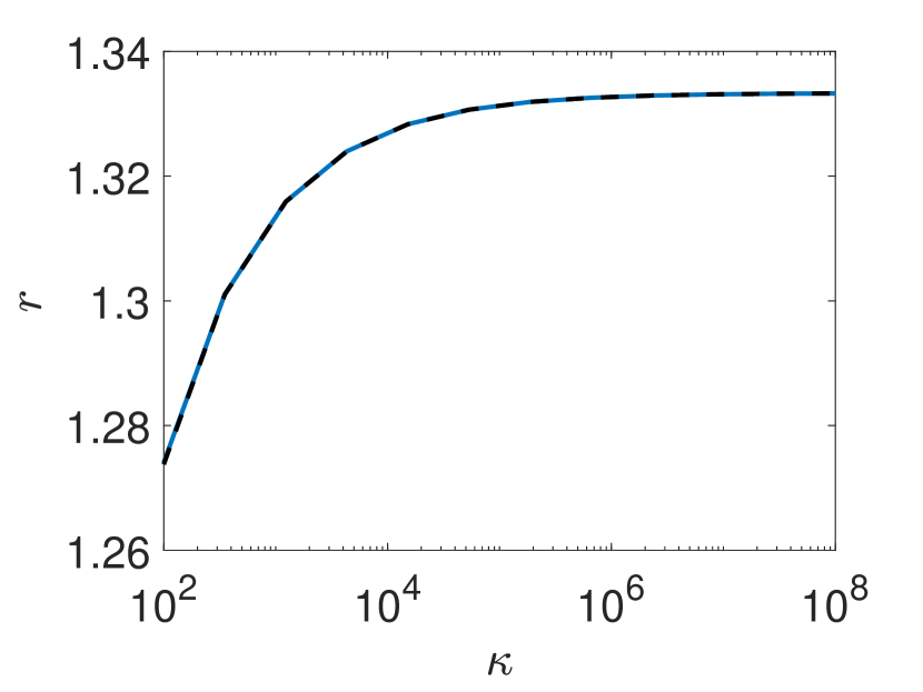
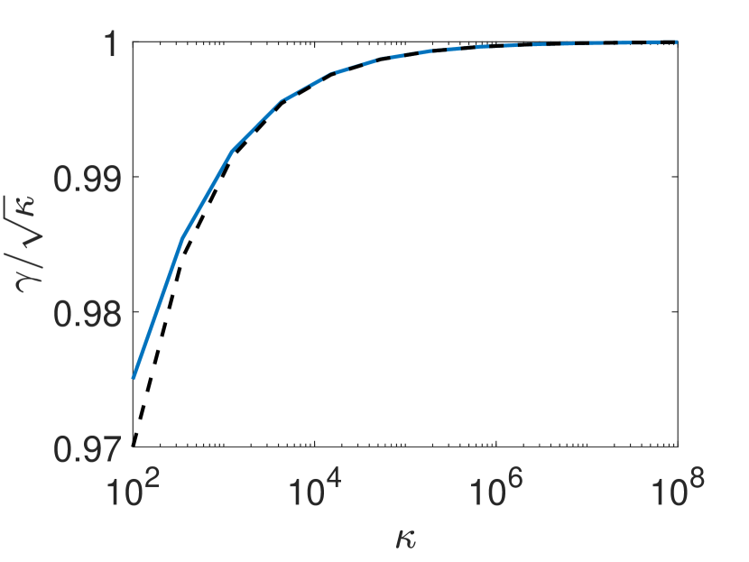
Figure 4: Convergence of the stochastic Nesterov algorithm with $\tilde{\alpha},\tilde{\beta},\eta$ given by (6.10) when $\rho_{0}=10$. On the left we have the convergence rate $r$, on the right we show, as a fraction of $\sqrt{\kappa}$, the value of $\gamma$ from (6.11). In the dashed lines we show the values when using the approximation $\gamma=\sqrt{\kappa}-(1/3)(1-\rho_{0}^{-1})$.

It remains to consider the $2\times 2$ matrix

$$T^{0}=\left[\begin{matrix}t_{11}&t_{12}\\ t_{12}&t_{22}\end{matrix}\right].$$

Following the approach for the deterministic Nesterov algorithm, we calculate $r$ and $p_{22}$ by imposing $\Delta=0$ and $(\partial/\partial p_{22})\Delta=0$ where $\Delta=\det(T^{0})$. Since $\Delta$ is a quadratic function of $p_{22}$, there is a unique value of $p_{22}$ which solves $(\partial/\partial p_{22})\Delta=0$. Then we have $p_{22}$ as a function of $\rho^{2}$ and it remains to solve $\Delta=\det(T^{0})$ for $\rho^{2}$ and check the following conditions:

$$t_{11}\leq 0\text{ and }t_{22}\leq 0,$$ (6.12a)

$$\widehat{P}+\frac{m}{2}\widehat{E}^{\textsf{T}}\widehat{E}\succ 0,$$ (6.12b)

$$p_{11}(\gamma-1)^{2}+2p_{12}(\gamma-1)+p_{22}\geq 0.$$ (6.12c)

The first of these along with having $t_{13}=t_{23}=t_{33}$ and $\Delta=0$ ensures that $T\preceq 0$. The second condition is an assumption in Theorem 6.1 which ensures that the Lyapunov function used upper bounds the Euclidean norm. The third condition is used to ensure that (6.4) holds.

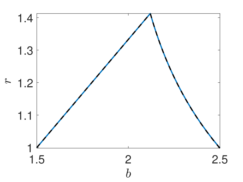
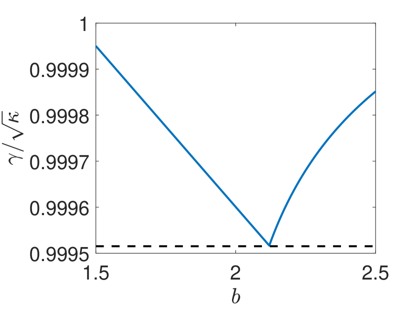
Figure 5: Convergence of the stochastic Nesterov algorithm with $\tilde{\alpha},\tilde{\beta},\eta$ given by (6.13), $\kappa=10^{6}$ and $\rho_{0}=10$. On the left we have the convergence rate $r$, on the right we show the optimal choice of $\gamma$ as a fraction of $\sqrt{\kappa}$. In the solid line we show the value of $r$, and the value of $\gamma$ resulting from $t_{33}=0$. In the dashed lines we show the values when $\gamma$ is set by (6.14).

It is convenient to express the variable $\rho$ determined by the procedure above in terms of a new variable $r$ as follows

$$\rho^{2}=1-r\frac{\sqrt{m}}{\rho_{0}\sqrt{L}}.$$

Note that $r=1$ corresponds to the rate obtained in [31] and that therefore values $r>1$ indicate an improved rate. In Figure 4 we show how $r$ varies as a function of $\kappa$ along with the associated value of $\gamma$ from (6.11). We see, for $\kappa$ large, $r$ converges to $4/3$ and hence $\gamma$ is approximately

$$\gamma\approx\frac{\sqrt{\kappa}-\rho_{0}^{-1}-\frac{1}{3}}{1-\frac{4}{3}\rho_{0}^{-1}\kappa^{-\frac{1}{2}}}\approx\sqrt{\kappa}-\frac{1}{3}(1-\rho_{0}^{-1}).$$

In the dashed line of Figure 4 we show the value of $r$ obtained if we use the approximation of $\gamma=\sqrt{\kappa}-({1}/{3})(1-\rho_{0}^{-1})$. We see that for all values of $\kappa$ considered we have $r>1$ and for large values of $\kappa$ that $r$ approaches $4/3$.

To leading order in $\kappa$ we have that $P$ matches the matrix $\widehat{\bar{P}}$ in the continuous deterministic setting, indeed

$$\widehat{P}\approx\frac{m}{2}\left[\begin{array}[]{cc}1&r\\ r&{r^{2}}/{2}\end{array}\right];$$

from this we see for $\kappa$ sufficiently large that (6.12c) holds.

Remark 6.3.

In the preceding analyis, we have chosen to use $\tilde{\alpha},\tilde{\beta}$ and $\eta$ as in [31] and set an alternative value for $\gamma$. When $\rho_{0}=1$, (6.8) is the same algorithm as (3.11) except with a different set of parameters, and using the parameters given by (6.10) corresponds to setting $\beta=(\sqrt{\kappa}-1)/(\sqrt{\kappa}+1)$. As discussed in Section 3, the choice $\beta=1-\sqrt{2/\kappa}$ allows to show an improved convergence rate. We obtain analogous behaviour to Section 3 by proceeding as above but using the parameter choice:

$$\tilde{\alpha}=\frac{1}{\rho_{0}\sqrt{\kappa}},\quad\tilde{\beta}=\frac{1-b\frac{1}{\rho_{0}\sqrt{\kappa}}}{1-\tilde{\alpha}},\quad\eta=\frac{1}{L\rho_{0}}.$$ (6.13)

Here $b$ is a new parameter to be chosen which is introduced to be analogous to the parameter $b$ in Section 3, the choice $b=2$ corresponds to the parameter choice (6.10) to leading order. As before, we can either use $\gamma$ obtained by solving $t_{33}=0$ for $\gamma$ or an approximation, which now is given by

$$\gamma=\frac{3\,\kappa^{-1/2}+\sqrt{\kappa}\,\rho_{0}-\sqrt{2}\,\kappa^{-1/2}-\frac{3\,\sqrt{2}}{2}+\rho_{0}-\sqrt{2}\rho_{0}}{\rho_{0}-\sqrt{2}\kappa^{-1/2}}.$$ (6.14)

By the same strategy as above, we establish convergence of $\lVert x-x^{\star}\rVert^{2}$ with rate $\rho^{2}$, for $\rho^{2}=1-r\kappa^{-1/2}\rho_{0}^{-1}$. In Figure 5 we show how $r$ depends on $b$. As in Figure 1, we see that $b=3\sqrt{2}/2$ gives $r=\sqrt{2}$ to leading order in $\kappa$.

Acknowledgements. PD and KCZ acknowledges support from the EPSRC gran tEP/V006177/1. JMS has been funded by Ministerio de Ciencia e Innovación (Spain), project PID2022-136585NB-C21, MCIN/AEI/10.13039/501100011033/FEDER, UE.

References

- [1] M. Betancourt, M. I. Jordan, and A. C. Wilson. On symplectic optimization. arXiv:1802.03653, 2018.
- [2] A. Bravetti, M. L. Daza-Torres, H. Flores-Arguedas, and M. Betancourt. Optimization algorithms inspired by the geometry of dissipative systems. arXiv:1912.02928, 2019.
- [3] G. J. Cooper and A. Sayfy. Additive methods for the numerical solution of ordinary differential equations. Mathematics of Computation, 35, 1980.
- [4] G. J. Cooper and A. Sayfy. Additive Runge-Kutta methods for stiff ordinary differential equations. Mathematics of Computation, 40, 1983.
- [5] A. B. Duncan, N. Nüsken, and G. A. Pavliotis. Using perturbed underdamped Langevin dynamics to efficiently sample from probability distributions. Journal of Statistical Physics, 169(6), 12 2017.
- [6] M. J. Ehrhardt, E. S. Riis, T. Ringholm, and C.-B. Schönlieb. A geometric integration approach to smooth optimisation: Foundations of the discrete gradient method. arXiv:1805.06444, 2018.
- [7] M. Fazlyab, A. Ribeiro, M. Morari, and V. M. Preciado. Analysis of optimization algorithms via integral quadratic constraints: nonstrongly convex problems. SIAM Journal on Optimization, 28(3):2654–2689, 2018.
- [8] G. Franca, M. I. Jordan, and R. Vidal. On dissipative symplectic integration with applications to gradient-based optimization. Journal of Statistical Mechanics: Theory and Experiment, 2021(4):043402, 2021.
- [9] F. Futami, T. Iwata, N. Ueda, and I. Sato. Accelerated diffusion-based sampling by the non-reversible dynamics with skew-symmetric matrices. Entropy, 23(8), 2021.
- [10] F. Futami, T. Iwata, N. Ueda, and I. Yamane. Skew-symmetrically perturbed gradient flow for convex optimization. volume 157 of Proceedings of Machine Learning Research, pages 721–736. PMLR, 2021.
- [11] C. R. Hwang, S. Y. Hwang-Ma, and S. J. Sheu. Accelerating diffusions. The Annals of Applied Probability, 15(2):1433 – 1444, 2005.
- [12] C. R. Hwang, R. Normand, and S. J. Wu. Variance reduction for diffusions. Stochastic Processes and their Applications, 125(9):3522–3540, 2015.
- [13] W. Krichene, A. Bayen, and P. L Bartlett. Accelerated mirror descent in continuous and discrete time. In Advances in Neural Information Processing Systems 28, pages 2845–2853. 2015.
- [14] M. Laborde and A. Oberman. A Lyapunov analysis for accelerated gradient methods: from deterministic to stochastic case. volume 108 of Proceedings of Machine Learning Research, pages 602–612. PMLR, 2020.
- [15] T. Lelièvre, F. Nier, and G. A. Pavliotis. Optimal non-reversible linear drift for the convergence to equilibrium of a diffusion. Journal of Statistical Physics, 152(2):237–274, 2013.
- [16] L. Lessard, B. Recht, and A. Packard. Analysis and design of optimization algorithms via integral quadratic constraints. SIAM Journal on Optimization, 26(1):57–95, 2016.
- [17] S. Ma, R. Bassily, and M. Belkin. The power of interpolation: Understanding the effectiveness of SGD in modern over-parametrized learning. volume 80 of Proceedings of Machine Learning Research, pages 3325–3334. PMLR, 2018.
- [18] A. Megretski and A. Rantzer. System analysis via integral quadratic constraints. IEEE Transactions on Automatic Control, 42(6):819–830, 1997.
- [19] M. Muehlebach and M. I. Jordan. A dynamical systems perspective on Nesterov acceleration. volume 97 of Proceedings of Machine Learning Research, pages 4656–4662. PMLR, 2019.
- [20] M. Muehlebach and M. I. Jordan. Optimization with momentum: Dynamical, control-theoretic, and symplectic perspectives. Journal of Machine Learning Research, 22(1), 2021.
- [21] Y. Nesterov. A method for solving the convex programming problem with convergence rate . Proceedings of the USSR Academy of Sciences, 269:543–547, 1983.
- [22] Y. Nesterov. Efficiency of coordinate descent methods on huge-scale optimization problems. SIAM Journal on Optimization, 22(2):341–362, 2012.
- [23] Y. Nesterov. Introductory Lectures on Convex Optimization: A Basic Course. Springer Publishing Company, Incorporated, 1 edition, 2014.
- [24] A. Orvieto and A. Lucchi. Shadowing properties of optimization algorithms. In Advances in Neural Information Processing Systems 32, pages 12692–12703. 2019.
- [25] B. T. Polyak and P. Shcherbakov. Lyapunov functions: An optimization theory perspective. IFAC-PapersOnLine, 50(1):7456 – 7461, 2017. 20th IFAC World Congress.
- [26] B.T. Polyak. Some methods of speeding up the convergence of iteration methods. USSR Computational Mathematics and Mathematical Physics, 4(5):1–17, 1964.
- [27] J. M. Sanz Serna and K. C. Zygalakis. The connections between Lyapunov functions for some optimization algorithms and differential equations. SIAM Journal on Numerical Analysis, 59(3):1542–1565, 2021.
- [28] D. Scieur, V. Roulet, F. R. Bach, and A. d’Aspremont. Integration methods and optimization algorithms. In Advances in Neural Information Processing Systems 30, pages 1109–1118, 2017.
- [29] B. Shi, S. S Du, W. Su, and M. I Jordan. Acceleration via symplectic discretization of high-resolution differential equations. In Advances in Neural Information Processing Systems, volume 32, pages 5744–5752, 2019.
- [30] W. Su, S. Boyd, and E. J. Candès. A differential equation for modeling Nesterov’s accelerated gradient method: Theory and insights. Journal of Machine Learning Research, 17(153):1–43, 2016.
- [31] S. Vaswani, F. Bach, and M. Schmidt. Fast and faster convergence of sgd for over-parameterized models and an accelerated perceptron. volume 89 of Proceedings of Machine Learning Research, pages 1195–1204. PMLR, 2019.
- [32] A. Wibisono, A. C. Wilson, and M. I. Jordan. A variational perspective on accelerated methods in optimization. Proceedings of the National Academy of Sciences, 113(47):E7351–E7358, 2016.
- [33] A. C. Wilson, B. Recht, and M. I. Jordan. A Lyapunov analysis of accelerated methods in optimization. Journal of Machine Learning Research, 22(113):1–34, 2021.
- [34] C. Zhang, S. Bengio, M. Hardt, B. Recht, and O. Vinyals. Understanding deep learning requires rethinking generalization. In International Conference on Learning Representations, 2017.