Encoding Domain Expertise into Multilevel Models for Source Location

Abstract

Data from populations of systems are prevalent in many industrial applications. Machines and infrastructure are increasingly instrumented with sensing systems, emitting streams of telemetry data with complex interdependencies. In practice, data-centric monitoring procedures tend to consider these assets (and respective models) as distinct – operating in isolation and associated with independent data. In contrast, this work captures the statistical correlations and interdependencies between models of a group of systems. Utilising a Bayesian multilevel approach, the value of data can be extended, since the population can be considered as a whole, rather than constituent parts. Most interestingly, domain expertise and knowledge of the underlying physics can be encoded in the model at the system, subgroup, or population level. We present an example of acoustic emission (time-of-arrival) mapping for source location, to illustrate how multilevel models naturally lend themselves to representing aggregate systems in engineering. In particular, we focus on constraining the combined models with domain knowledge to enhance transfer learning and enable further insights at the population level.

L.A. Bull et al.

1 Introduction

Engineering systems and infrastructure are increasingly equipped with sensors, often providing streams of telemetry data. As the number of instrumented systems grows, population data become available [1]. While machine populations clearly differ from the natural examples in ecology, epidemiology, and behavioural science, the same statistical methods can be used when representing the interactions of artificial systems [2].

In this article, we consider multilevel (or hierarchical) models [3], a family of methods that are particularly suited to population studies since the associated data naturally exhibit a hierarchical structure. As an engineering example, consider turbines in a wind farm. Although the wind-power relationships may vary depending on the unique environment of each machine, the wind speed at which they start generating power, and the limiting power output, should be the same for all members of the group, provided that they are the same specification and functioning correctly [4].

A multilevel model can represent the interdependencies of such structured data, as nested groups of models can pool information. This extends the value of data by sharing parameters either (i) directly, or (ii) indirectly with parameters that depend on some common, latent variables. A conceptual introduction of these models as mulitask learners can be found in [5]. Most interestingly, by modelling intertask relationships (between machines) alternative insights can be extracted from the statistical model, which can help to inform simulation, control, and maintenance.

We consider an example in this work, where the population members are represented by a sequence of 28 Acoustic Emission (AE) experiments, originally from [6]. In each experiment, the arrival time of waves propagating through a complex plate geometry is recorded. For each dataset, a 2D map of the arrival times is learnt through regression. Despite distinct experiment designs, the metal plate remains consistent (the medium through which waves propagate) suggesting that the models share certain characteristics. Importantly, we show that by analysing these datasets collectively, as a population, additional insights can be extracted from the test campaign. We capture how characteristics of the 2D map vary, allowing us to predict hyperparameters of the response surface for experimental designs which are absent from the training data. In essence, we can extrapolate or interpolate in the model space.

These insights have significant implications practically since the intertask models can be used to predict the characteristics of the response for new, previously unobserved experimental designs. Such model predictions alleviate the requirement of extensive training data in new domains, by sharing information from similar experiments. The result is an interpretable and explainable approach to transfer learning for engineering experiments.

1.1 Layout

Section 2 introduces the AE data, the experimental campaign, and their multilevel interpretation. Section 3 uses Gaussian Process regression to encode domain expertise via model design and prior formulation, for a single experiment. Section 4 extends the model to represent data from the full test campaign in a joint inference, investigating different model assumptions and the associated intertask relationships. Section 5 assesses the predictive performance and utilises the model for transfer learning, discussing various assumptions. Section 6 offers concluding remarks. While the experimental data in this work are not currently available to share, python and stan code will be shared, via https://github.com/labull/EngineeringPatternRecognition.

1.2 Related Work & Contribution

To improve interpretability and ensure meaningful outputs from data-driven models, the inclusion of physical insight within machine learning methods is becoming increasingly popular, with overviews found in [7, 8]. These approaches are often referred to as physics-informed machine learning, since they utilise both data and explanatory physics to improve modelling when compared to either approach independently. Some examples include physics-guided loss functions [9], vector field constraints [10], and the inclusion of governing differential equations [11].

Contribution

In the context of AE (time of arrival) mapping, previous work of (coauthors) Jones et al. [12] considered how domain knowledge can be encoded in Gaussian Process (GP) models via boundary condition constraints, applied to the kernel function for a single experiment. Here, we extend the work to represent multiple experiments, allowing us to encode domain expertise at the systems level and infer intertask relationships for a series of tests. Our key contribution is, therefore, the ability to encode physics-based knowledge between tasks, as well as within tasks. Rather than a single experiment, the resultant model represents variations over an entire experimental campaign: this allows for simulation and (hyper) parameter prediction at previously unobserved experimental designs (in this case, sensor separation).

We adopt a multilevel modelling approach, which is increasingly utilised in the engineering literature. An early monitoring example is presented by Huang et al. [13] and Huang and Beck [14], where multiple correlated regression tasks are utilised for modal analysis. A shared sparsity profile is inferred for tasks relating to measurement channels to improve damage detection by considering the correlation between damage scenarios or adjacent sensors. More recent applications include Di Francesco et al. [15] who use multilevel models to represent corrosion progression given evidence from multiple locations, and Papadimas and Dodwell [16], where the results from materials tests (i.e. coupon samples) are combined to inform the estimation of material properties. Similar to Papadimas and Dodwell [16], our work considers an experimental campaign, but rather than infer the higher-level representation as a global estimate of a single experiment, we introduce inter-task explanatory variables. In turn, the model can represent task variations as functions, rather than uni-modal sampling distributions.

On a related theme, Hughes et al. [17] recognise structures and their populations as nested hierarchies, proposing a convenient formulation for decision analyses. Sedehi et al. [18] also present interesting work to encoding physics into hierarchical GPs, where time-history measurements are partitioned into multiple segments to create longitudinal data, accounting for temporal variability and addressing the non-stationarity of the measured responses for a single structure.

2 The Acoustic Emission Experiments

Acoustic Emissions (AE) are ultrasonic signals released within a material as its internal structure undergoes some irreversible change. The driving mechanisms often relate to the initiation and growth of damage, so monitoring AE signals can serve to assess the condition of materials and structures [19]. As emissions propagate through a material from the point of origin, differences in the time of arrival at separate sensors (in an array) can be used for triangulation (or trilateration) to enable source location [20]. From a damage monitoring perspective, source location provides an operator with more insight to make better maintenance and planning decisions.

One strategy for localising AE signals involves learning the map of the arrival times across the surface of interest [21]. That is, the forward mapping from AE source location $\mathbf{x}_{i}$ to the measured difference in time-of-arrival ($\Delta$ToA) for a given sensor pair,

$$y_{i} =f(\mathbf{x}_{i})+\epsilon_{i}$$ (1)

where $y_{i}$ is some noisy observation of $\Delta$ToA with additive observation noise $\epsilon_{i}$. In this paper, we consider data from experiments by Hensman et al. [6] concerning an aluminium plate-like structure shown in Figure 1.

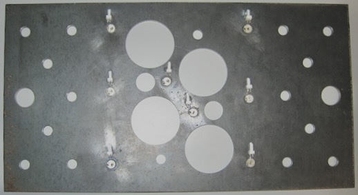
Figure 1: Image of plate used in AE experiments.

Artificial AEs were excited by thermoelastic expansion generated with an incident laser pulse, with the signals captured at 8 piezoceramic (Sonox P5) sensors mounted to the surface of the plate, visible in Figure 1 and shown by black markers in Figure 2. The sensors operate by converting surface displacements resulting from the AE stress waves into electrical energy, allowing the ultrasonic signals to be captured digitally. There are a total of $N=2227$ possible source locations, shown by blue markers in Figure 2. The time of arrival for each of the 8 sensors was extracted following standard practice, using an autoregressive form of the Akaike Information Criterion (AIC) [6].

Difference in time-of-arrival ($\Delta$ToA)

Let the arrival time of AE $i$ at sensor $j$ be denoted $A_{ij}\quad\forall j\in\{1,2,\ldots,8\}$. The difference in time-of-arrival ($\Delta$ToA) is then the difference between any two sensors. Since there are 8 sensors, there are 28 pairwise combinations and associated maps (8C2). Each pair generates a different $f$ (we will distinguish these with notation later). For example, the pair (3, 5) would present the scalar output $y_{i}\in\mathbb{R}$,

$$y_{i}=A_{i3}-A_{i5}$$

The input vectors $\mathbf{x}_{i}\in\mathbb{R}^{2}$ are the locations (length vs. width),

$$\mathbf{x}_{i}=\{x^{(1)}_{i},x^{(2)}_{i}\}$$

where {0, 0} is the bottom left corner of the plate. Figure 2 (left) shows the data associated with the sensor pair (3, 5) while Figure 3 shows all pairs.

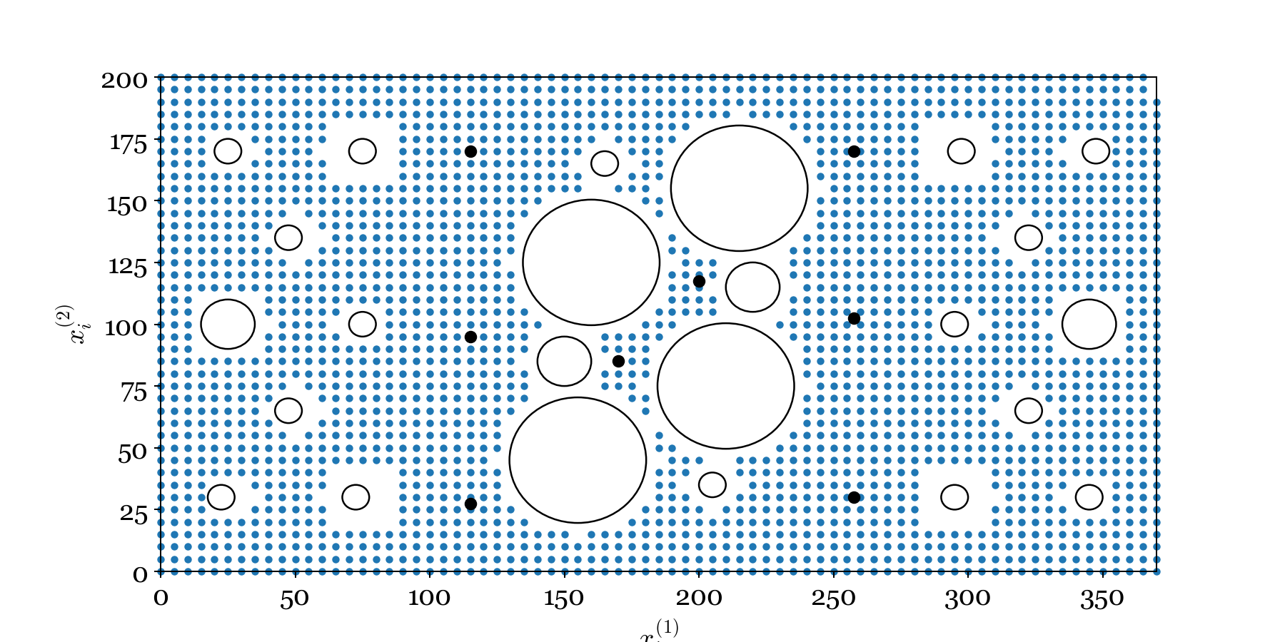
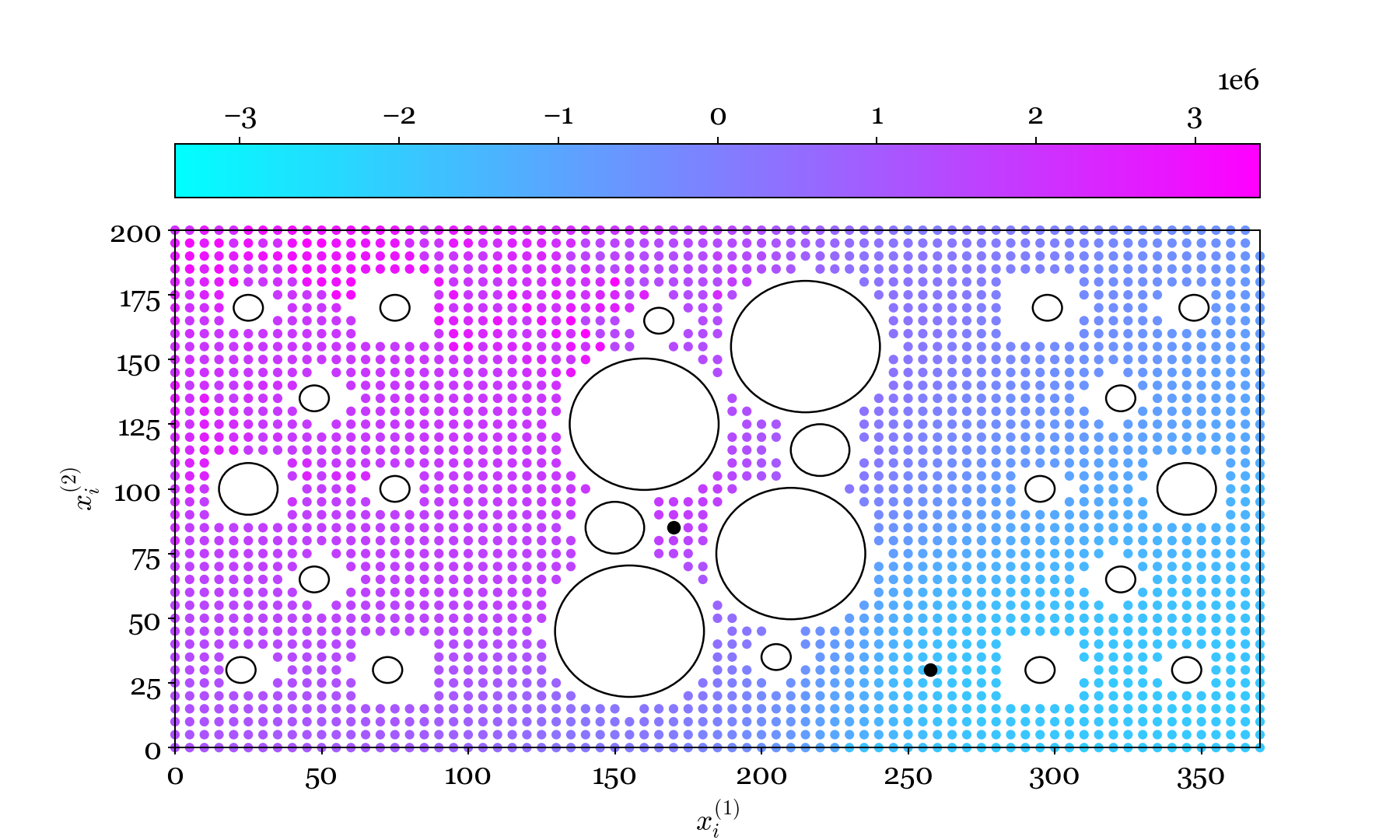
Figure 2: Left: all possible source locations (blue $\bullet$) and sensor locations (black $\bullet$). Right: heatmap of the $\Delta$ToA (response $y_{i}$) with respect to locations (inputs $\mathbf{x}_{i}=\{x^{(1)}_{i},x^{(2)}_{i}\}$).

A note on normalisation

Figure 3 plots $N=100$ training data for each sensor pair combination, sampled uniformly from each domain. We then normalise inputs with respect to the longest edge, such that the plate’s length is unity. This scaling maintains approximately the same relative smoothness of the map in each direction, i.e. one length scale for both dimensions.

Rather than normalising the response for each plate independently, we (z-score) normalise response with respect to all 28 sensor pairings. This maintains the relative structure between experiments (sensor pairs) in the combined data. More specifically, a global normalisation of the outputs is essential to prevent interesting differences (between tests) from being scaled out of the data.

Why multilevel?

In the context of this work, each map and sensor pair corresponds to a distinct but related environment: each referred to as an experiment, with an associated task learnt by the regression. These collected environments are visualised in Figure 3. If we learn these maps collectively, in a combined inference, the model should capture variations between each sensor pair, representing further insights from the experimental campaign, which emerge at the systems level.

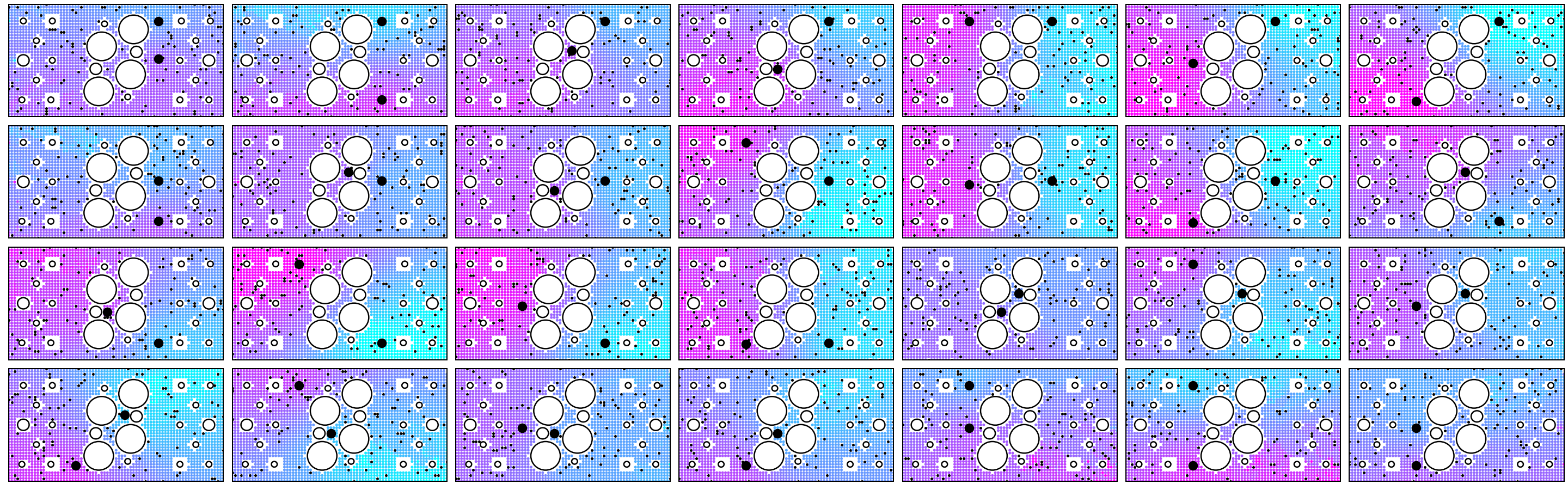
Figure 3: Heatmaps of the measured $\Delta$ToA ($y_{i}$) with respect to locations ($\mathbf{x}_{i}$) for all sensor combinations. Large black markers plot sensor pairs, while smaller black markers plot training observations. The remaining data are used to test out-of-sample performance.

3 Representing AE Maps with Gaussian Processes Regression

GPs are used to represent each of these experiments since they offer a flexible tool for regression with natural mechanisms to encode engineering knowledge and domain expertise. First, we consider one domain at a time (Section 4 extends the model to consider all experiments in a combined inference). The observation noise $\epsilon_{i}$ is assumed to be normally distributed,

$$y_{i}=f(\mathbf{x}_{i})+\epsilon_{i},\qquad\epsilon_{i}\sim\textrm{N}(0,\sigma_{i})$$ (2)

In fact, $\epsilon_{i}$ will represent more than observation noise, since it captures the combined uncertainty of the $\Delta$ToA extraction, from the raw time series data. Still, as with previous work [21, 22, 12, 6] we found this representation works well in practice.

Rather than suggest a parametrisation of $f$ we assume that it has a nonparametric GP prior distribution,

$$\boldsymbol{\theta} \sim p(\boldsymbol{\phi})$$ (3)

$$f(\mathbf{x}_{i}) \sim\textrm{GP}\left(m_{f}(\mathbf{x}_{i};\boldsymbol{\theta}),\;k_{f}(\mathbf{x}_{i},\mathbf{x}_{j};\boldsymbol{\theta})\right)$$ (4)

The prior over $f$ is specified by its mean $m_{f}$ and covariance $k_{f}$ functions, where $\boldsymbol{\theta}$ is the set of collected hyperparameters. These hyperparameters are sampled from the higher level distribution $p(\boldsymbol{\phi})$ whos prior is parametrised by constants in $\boldsymbol{\phi}$. The mean and covariance of the prior offer natural mechanisms to encode knowledge of the expected functions given domain expertise, before any data are observed. The covariance determines the expected correlation between outputs – influencing process variance, and smoothness – while the mean represents the prior expectation of the structure of the functions.

A function sample from the GP, denoted $\mathbf{f}$, is multivariate normal for any finite set of $N$ observations,

$$\mathbf{f} \sim\textrm{N}\left(\mathbf{m_{f}},\;\mathbf{K_{f}}\right)$$ (5)

y $$\sim\textrm{N}(\textbf{f},\boldsymbol{\sigma})$$ (6)

$$\mathbf{K_{f}}[i,j] \triangleq k_{f}(\mathbf{x}_{i},\mathbf{x}_{j};\boldsymbol{\theta})$$ (7)

$$\mathbf{m_{f}}[i] \triangleq m_{f}(\mathbf{x}_{i})$$ (8)

Since the observation model is assumed Gaussian, we can avoid sampling $\mathbf{f}$ entirely by combining the GP kernel $\mathbf{K_{f}}$ with the observation noise vector $\boldsymbol{\sigma}$, to describe the likelihood function,

$$\mathbf{y} \sim\textrm{N}(\mathbf{m_{f}},\mathbf{K_{f}}+\operatorname{diag}(\boldsymbol{\sigma}^{2}))$$ (9)

Following [21] we use a zero-mean and Matérn $3/2$ kernel function $k_{f}$ for the covariance function,

$$\mathbf{m_{f}}[i] =0$$ (10)

$$\mathbf{K_{f}}[i,j] =\alpha^{2}\left(1+\frac{\sqrt{3}\left|\mathbf{x}_{i}-\mathbf{x}_{j}\right|}{l}\right)\exp\left(-\frac{\sqrt{3}\left|\mathbf{x}_{i}-\mathbf{x}_{j}\right|}{l}\right)$$ (11)

The zero-mean function is justified since the complex plate geometry prevents the specification of a parametrised mean. In the absence of this information, a zero mean is sufficient in practice, since the GP alone is flexible enough to model arbitrary trends. Two hyperparameters are introduced via the kernel $k_{f}$ (11) such that $\boldsymbol{\theta}=\{\alpha,l\}$. The process variance $\alpha$ encodes the magnitude of function variations around the expected mean. The length scale $l$ encodes how much influence a training observation has on its neighbouring inputs, it represents the smoothness of the approximating family of functions.

3.1 Heteroscedastic noise

In the experiments, we expect the scale of the observation noise $\sigma_{i}$ to increase at the extremities of the plate [22]. In other words, the magnitude of the noise is input-dependant: it is not statistically identical over the whole domain (i.e. it is not homoscedastic). Such input-dependent noise can be represented with a heteroscedastic regression. Heteroscedasticity is implemented with another GP in a combined model, mapping the inputs $\mathbf{x}_{i}$ to the variance of the observation noise $\sigma_{i}$. This introduces the noise-process $r$, where the prior utilises a constant mean function and another Matérn $3/2$ kernel function (with its own set of hyperparameters). Therefore, a finite sample from the noise process is distributed as follows,

r $$\sim\textrm{N}\left(\mathbf{m_{r}},\mathbf{K_{r}}\right)$$ (12)

$$\boldsymbol{\sigma} =\exp(\mathbf{r})$$ (13)

$$\mathbf{m_{r}}[i] =m_{r}$$

$$\mathbf{K_{r}}[i,j] =\alpha_{r}^{2}\left(1+\frac{\sqrt{3}\left|\mathbf{x}_{i}-\mathbf{x}_{j}\right|}{l_{r}}\right)\exp\left(-\frac{\sqrt{3}\left|\mathbf{x}_{i}-\mathbf{x}_{j}\right|}{l_{r}}\right)$$ (14)

Samples from $r$ are exponentiated to define $\boldsymbol{\sigma}$ since the noise variance must be strictly positive (note that, untransformed, a GP will map to any real number). The exponential transformation requires a constant mean function in this case, otherwise, the prior of the expected noise variance is limited to $\exp(0)=1$. The additional hyperparameters from the noise process are now included in the total set $\boldsymbol{\theta}$,

$$\{m_{r},\alpha_{r},l_{r}\}\in\boldsymbol{\theta}$$

3.2 Prior formulations

One should encode prior knowledge of the AE maps as prior distributions over the higher-level variables $\boldsymbol{\theta}\sim p(\boldsymbol{\phi})$. The hyperparameters of the GP are sampled from these distributions, which characterise the expected variation, smoothness, and noise of the maps. The following $p(\boldsymbol{\phi})$ structure is adopted,

$$\boldsymbol{\theta}=\{l,\alpha, m_{r},\alpha_{r},l_{r}\},\qquad\boldsymbol{\theta}\sim p(\boldsymbol{\phi})$$

$$l \sim\textrm{Gamma}(2,1)$$ (15)

$$\alpha \sim\textrm{Half-Normal}(1)$$ (16)

$$m_{r} \sim\textrm{N}(-0.9,1)$$ (17)

$$l_{r} \sim\textrm{Gamma}(2,1)$$ (18)

$$\alpha_{r} \sim\textrm{Half-Normal}(2)$$ (19)

The constants on the RHS correspond to $\boldsymbol{\phi}$, and they are specified based on intuitition. In view of the combined normalised space and our (basic) domain knowledge, they are set as weakly informative with distributions (15)-(19) explained below.

Recall that the inputs are normalised between [0, 1] with respect to the longest side. Since we expect relatively smooth $\Delta$ToA map $(f)$ and noise process $(r)$ we encode this intuition via Gamma distributed $l$ and $l_{r}$ which have their mode at 1. The output is z-score normalised, so we expect the process variance $\alpha$ should be a little less than unity (shrunk further by outliers). For a half-normal distribution with a unit scale, the expectation is,

$${\textrm{E}[\alpha]}=\frac{1\sqrt{2}}{\sqrt{\pi}}={0.8}$$ (20)

Then, a signal-to-noise ratio of 10 is assumed, in terms of expected scale,

$$\frac{\textrm{expected process noise}}{\textrm{expected observation noise}} =\frac{\textrm{E}[\alpha]}{\textrm{E}[\boldsymbol{\sigma}]}=\frac{\textrm{E}[\alpha]}{\textrm{E}[\exp(r)]}=\frac{\textrm{E}[\alpha]}{\exp(\textrm{E}[\mathbf{m_{r}}])}$$ (21)

$$=\frac{{1\sqrt{2}}\times{\pi}^{-0.5}}{\exp(-2.5)}=\frac{0.8}{0.08}$$ (22)

A vague prior is defined for $\alpha_{r}$, which indicates high variance in the noise process $r$, to reflect weak a priori knowledge,

$${\textrm{E}[\alpha_{r}]}=\frac{2\sqrt{2}}{\sqrt{\pi}}={1.6}$$ (23)

We assume this high scale for the noise process, since it is known that measurement noise increases dramatically at the extremities of the plate, far from the centroid of sensor pairs [22].

3.3 Inference and prediction

To identify the model and make predictions, one can infer the posterior distribution for latent variables $p(\boldsymbol{\Theta}\mid\mathbf{y})$ by conditioning the joint distribution (which encodes domain expertise via the model and the prior specification) on the training data $\mathbf{y}$. We use $\boldsymbol{\Theta}$ to generically collect all (unobservable) latent variables, including functions, parameters, and hyperparameters. The joint distribution is written as the product of two densities, referred to as the likelihood $p(\mathbf{y}\mid\boldsymbol{\Theta})$ (or the data distribution) and the prior $p(\boldsymbol{\Theta})$,

$$p(\mathbf{y},\boldsymbol{\Theta})=p(\mathbf{y}\mid\boldsymbol{\Theta})p(\boldsymbol{\Theta}\;;\;\boldsymbol{\phi})$$ (24)

During model design, we have specified the likelihood with (9) and the prior throughout (15)-(19). Applying the property of conditional probability to (24) we arrive at Baye’s rule and an expression for the posterior distribution,

$$p(\boldsymbol{\Theta}\mid\mathbf{y})=\frac{p(\mathbf{y}\mid\boldsymbol{\Theta})p(\boldsymbol{\Theta})}{p(\mathbf{y})}$$ (25)

While (25) is a straightforward application of conditioning [5], in practice, the evaluation of the denominator (i.e. the marginal likelihood or evidence) is non-trivial. It is specified by the following integral, which is intractable for most prior-likelihood combinations,

evidence: $$p(\mathbf{y})=\int p(\mathbf{y},\boldsymbol{\Theta})\;d\boldsymbol{\Theta}=\int p(\mathbf{y}\mid\boldsymbol{\Theta})p(\boldsymbol{\Theta})\;d\boldsymbol{\Theta}$$ (26)

The integral (26) is feasible for a subset of likelihood-prior distributions, known as conjugate pairs [3]. In many practical applications, however, it becomes increasingly hard to justify the model and prior choices that lead to conjugacy. In our case, the prior formulation $p(\boldsymbol{\theta}\mid\boldsymbol{\phi})$ required for a multilevel representation leads to an intractable (26).

A number of approximate Bayesian methods are used with non-conjugate models. Here, we utilise a sampling-based solution, inferring the parameters using MCMC and the no U-turn implementation of Hamiltonian Monte Carlo [23]. The models are implemented in the probabilistic programming language Stan [24].

When predicting new (previously unobserved) data $\mathbf{\tilde{y}}$ one (empirically) integrates out $\boldsymbol{\Theta}$ from the following product,

$$p(\mathbf{\tilde{y}}\mid\mathbf{y}) =\int p(\mathbf{\tilde{y}}\mid\boldsymbol{\Theta})p(\boldsymbol{\Theta}\mid\mathbf{y})\,d\boldsymbol{\Theta}$$

For GP variables $\{f,r\}$, the distribution used to predict new inputs has an analytical solution when the hyperparameters $\boldsymbol{\theta}$ are fixed. For the $f$-process, this would be $p(\mathbf{\tilde{y}}\mid\mathbf{y},\boldsymbol{\theta}_{s})$ where $\boldsymbol{\theta}_{s}$ represents a sample from the approximated posterior distribution. The analytical solution is then defined by conditioning a joint Gaussian, e.g. $p(\mathbf{\tilde{y}},\mathbf{y}\mid\boldsymbol{\theta}_{s})$, on the training variables. The relevant identity is provided in Appendix A.

For the (3,5) sensor pair, a random sample of $N=100$ observations is used for training, and the rest are set aside as test data. Following inference and prediction, Figure 4 plots the mean of the posterior predictive distribution for the two-dimensional map over the plate. To visualise the predictive variance and its heteroscedastic nature, a random slice is taken along the length of the map, and also plotted in Figure 4.

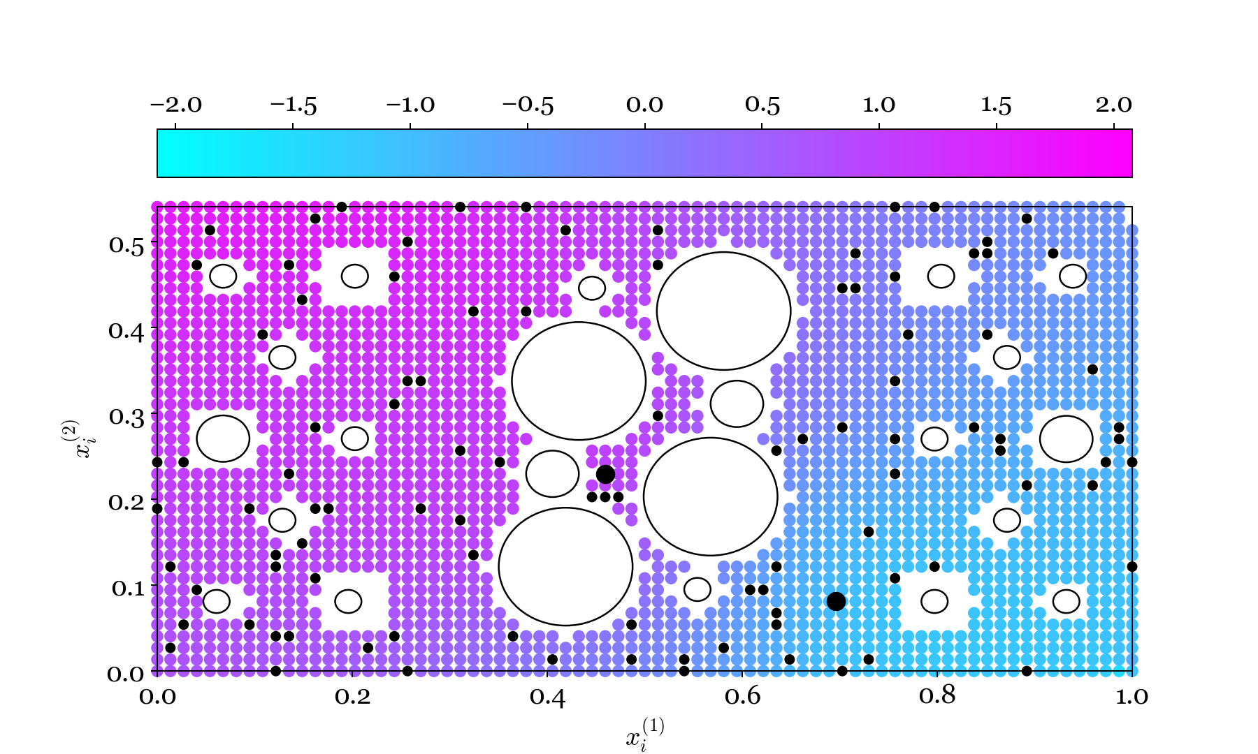
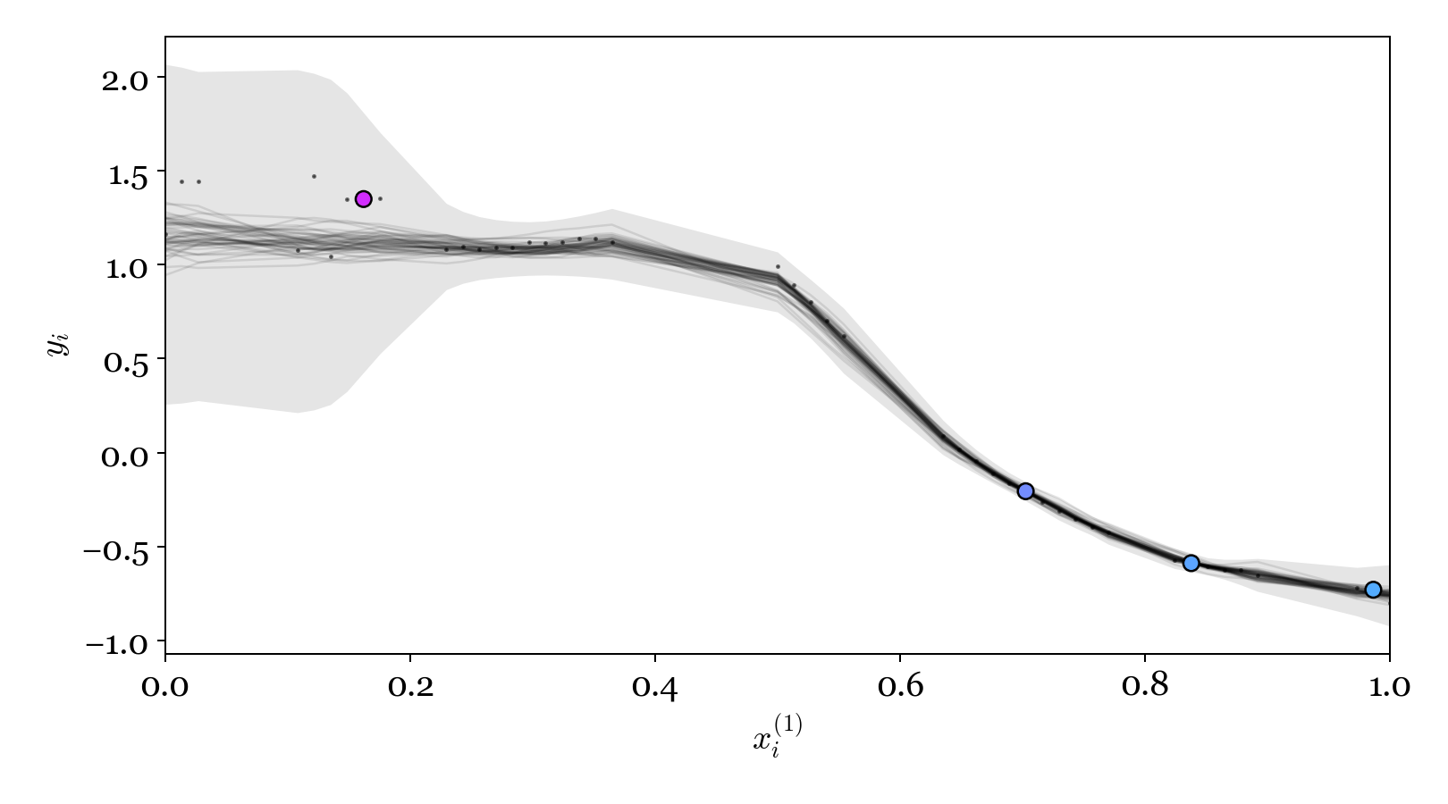
Figure 4: The inferred (3,5) mapping over the plate (left) and a length-wise slice to visualise the heteroscedastic noise (right).

4 Multilevel Representations

To conceptualise the hierarchical structure of the experimental data, we learn all 28 independent GPs (rather than sensor pair (3, 5) only). Each pairwise map is distinguished with an additional index $k\in\{1,2,\ldots,28\}$ so that the set of all maps is given by,

$$\{f_{k}\}^{K}_{k=1}$$

Throughout, we use the same test-train split of $N=100$ random samples from each domain, visualised in Figure 3. Following inferences, we plot and investigate hyperparameter variations of the independent models. Figure 5 shows samples from the posterior distributions $p(\boldsymbol{\theta}\mid\mathbf{y}_{k})\;\forall k$. Since the data are not shared between the experiments, with each task learnt independently, these models are considered single-task learners (STL) [5]. The plots are typical of longitudinal or panel data [3] (in this case, for the hyperparameters) where the task-specific $\boldsymbol{\theta}$ appear to be sampled from some higher-level generating distribution. In some sense, the experiment-specific models are perturbations around an average (higher-level model). An intuitive concept, since all experiments concern the same plate, despite the varying experimental design (sensor placement).

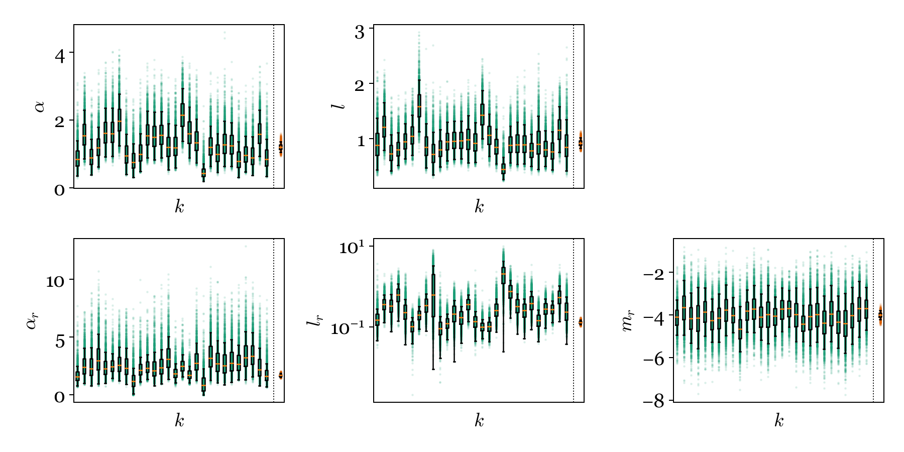
Figure 5: Posterior distribution of hyperparameters for independent GPs of each experiment (STL, green), compared to sharing hyperparameters (the prior) between all experiments (MTL A, orange). Top row: $f$-process hyperparameters (AE map). Bottom row: $r$-process hyperparameters (heteroscedastic noise).

4.1 (Method A) K GPs, one prior

In a combined inference, one simple way to share information between tests assumes that the smoothness $l$ and process variance $\alpha^{2}$ of all $\Delta$ToA maps $\{f_{k}\}$ is consistent. In other words, the GPs for each experiment are sampled from a shared prior,

$$\{\mathbf{f}_{k}\}_{k=1}^{K} \sim\textrm{N}\left(\mathbf{m_{f}},\;\mathbf{K_{f}}\right)$$

Same for the noise process $r_{k}$,

$$\{\textbf{r}_{k}\}_{k=1}^{K} \sim\textrm{N}\left(\mathbf{m_{r}},\mathbf{K_{r}}\right)$$

While this partial pooling [3] will likely improve inference compared to $K$ independent learners, we know that the assumptions are oversimplified – it is unlikely that the independent posterior samples (Figure 5, green) are estimating the same parameter since there are differences in the design of each experiment. The question is whether the assumption above provides a sufficient model.

Considering the above, distinct GPs $\{f_{k}\}$ sampled from a shared prior $\boldsymbol{\theta}$ are presented as a benchmark – multitask learning method A (MTL A). The resultant hyperparameter posterior distributions are shown by orange markers in Figure 5. These effects are typical of pooled estimates, assuming each experiment estimates a single underlying parameter. Caution is required, as when this assumption is inappropriate, it misrepresents the population variance.

4.2 (Method B) Hyperparameter modelling

A more intuitive generating process considers that certain hyperparameters are conditional on the experimental setup, rather consistent, to better represent the differences between each test. We can extend the notation of (3) with a $k$-index to reflect this,

$$\boldsymbol{\theta}_{k} \sim p(\boldsymbol{\phi})$$ (27)

$$\boldsymbol{\theta}_{k} \triangleq\{\alpha_{k},l_{k}\}$$

Distinct variables are considered for the $\mathbf{K_{f}}$ kernel only ($\alpha_{k}$ and $l_{k}$) since these are easier to interpret and relate to domain knowledge, especially if the plate had represented a simple geometry – this choice also helps to constrain the model design. Having a distinct set $\boldsymbol{\theta}_{k}$ allows the characteristics of the map to vary between each experiment: this should be expected since they are different experimental designs. The higher-level sampling distribution $p(\boldsymbol{\phi})$ remains shared between all experiments (and leant from pooled data to share information). We now consider modifications to the prior model $p(\boldsymbol{\theta}_{k}\mid\boldsymbol{\phi})$ to encode knowledge and domain expertise of the intertask relationships, i.e. between the experiments.

Beyond exchangeable experiments

When specifying a new prior model $p(\boldsymbol{\theta}_{k}\mid\boldsymbol{\phi})$ it is important to consider whether the experiments are exchangeable [3]. Here, they would be considered exchangeable if no information is available to distinguish the $\boldsymbol{\theta}_{k}$’s from one another. In other words, we cannot order the set $\{\boldsymbol{\theta}_{k}\}_{k=1}^{k}$ (presented Figure 5) such that patterns are revealed in the latent variables.

However, since we know about the design of the AE experiments, there are a few possibilities. We select the most simple description here – sensor separation – as an explanatory variable, to reorder the models beyond exchangeability. Sensor separation $\delta S_{k}$ is defined as the Euclidean distance between any two of the eight $\binom{2}{8}$ possible sensor locations $\mathbf{\hat{S}}=\{\mathbf{\hat{s}}_{1},\mathbf{\hat{s}}_{2},\ldots\mathbf{\hat{s}}_{8}\}$,

$$\delta S_{k}=\lvert\mathbf{\hat{s}}_{g}-\mathbf{\hat{s}}_{h}\rvert\quad\forall\quad\textrm{pairs from}\;\mathbf{\hat{S}}$$ (28)

i.e. the vector $\boldsymbol{\delta S}$ will be length $K=\binom{2}{8}=28$. The simple pattern we expect is that process variance $\alpha_{k}$ will decrease for sensor pairs that are closer. In other words, the variation in the $\Delta$ToA output should be greater for sensors that are further apart, since the AE signals have the potential to travel further.

Figure 6 plots the posterior distributions $\boldsymbol{\theta}$ (given only $\mathbf{y}_{k}$) with respect to $\delta S_{k}$ for the independent models from Figure 5. These samples indicate parameter relationships that we hope to learn with the higher-level model $p(\boldsymbol{\theta}_{k}\mid\boldsymbol{\phi})$. (Note that Figure 6 samples correspond to latent variables and not observations.)

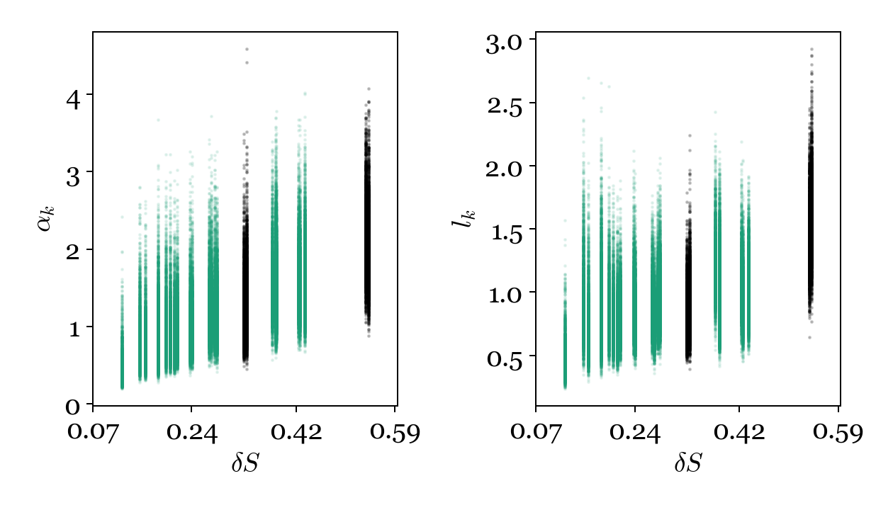
Figure 6: Ordering the hyperparameters of the experiments $\boldsymbol{\theta}_{k}$ with respect to sensor separation $\delta S_{k}$.

As expected, the process variance $\alpha_{k}$ increases with sensor separation. The length scale $l_{k}$ presents a similar trend: we believe this appears for smaller sensor spacing as the noise floor (observation noise as well as parameter uncertainty) is larger compared to the magnitude of the response variations ($\alpha_{k}$). In turn, the influence of each training observation on its neighbours is reduced.

Figure 5 also highlights the hold out experiments, represented by black markers (rather than green). Herein, the data for the hold-out tests are not used when training, to test interpolation and extrapolation in the hyperparameter space for the multilevel models.

Intertask GPs

Like the input-dependent noise process ($r$) the variation of the hyperparameters (of $\mathbf{K_{f}}$) can be represented with another function, which, in this case, is task-dependent (i.e. experiment-dependent). That is, the hyperparameters of AE map $f$ are sampled from higher-level functions, denoted $\{g,h\}$,

$$\boldsymbol{\theta} \sim p(\boldsymbol{\phi})$$ (29)

$$(\alpha)\quad\textrm{g-process}:\quad g(\delta S_{k}) \sim\textrm{GP}\left(m_{g}(\delta S_{k};\boldsymbol{\theta}),\;k_{g}(\delta S_{k},\delta S_{l};\boldsymbol{\theta})\right)$$ (30)

$$(l)\quad\textrm{h-process}:\quad h(\delta S_{k}) \sim\textrm{GP}\left(m_{h}(\delta S_{k};\boldsymbol{\theta}),\;k_{h}(\delta S_{k},\delta S_{l};\boldsymbol{\theta})\right)$$ (31)

where hyperparameter functions vary (between tasks) with respect to sensor separation $\delta S_{k}$ for the 24 training experiments,

g $$\sim\textrm{N}\left(\mathbf{m_{g}},\mathbf{K_{g}}\right)$$ (32)

$$\alpha_{k} =\textrm{softplus}(g_{k})\qquad\forall k\in\textrm{train}$$ (33)

h $$\sim\textrm{N}\left(\mathbf{m_{h}},\mathbf{K_{h}}\right)$$ (34)

$$l_{k} =\textrm{softplus}(h_{k})\qquad\forall k\in\textrm{train}$$ (35)

$$\boldsymbol{\theta}_{k} \triangleq\{\alpha_{k},l_{k}\}$$

Each GP is transformed to be strictly positive, as the hyperparameters they predict must be greater than zero. While the exponential function was used for this purpose with the noise-process $r$ (13) here we favour the softplus transformation [25] since it can be specified to provide a direct map over the inputs of interest, aiding the interpretability of the parameter models $\{g,h\}$. The exponentiated transformation is maintained for the lower-level GPs $f_{k}$ since it provided more stable inferences.

Priors

The noise process prior distributions are set as before (17)–(19) while the AE map priors are sampled from GPs (33)–(35), whose hyperparameters are added to $\boldsymbol{\theta}$. We use the same Matérn 3/2 kernel for the higher-level GPs, however, in this case, we use a linear mean function (with slope $m$ and gradient $c$). The linear mean allows us to encode domain knowledge of a positive gradient for the expected intertask functions via the GP prior. The conditional posterior predictive distributions of $\{g,h\}$ then provide intertask relationships learnt from the collected data (while only observing data as inputs on the lowest level $f$). The additional hyperparameters for the shared (global) sampling distributions are,

$$\{\alpha_{g},l_{g},\alpha_{h},l_{h},m_{g},c_{g},m_{h},c_{h}\}\in\boldsymbol{\theta}$$

Where $m$ and $c$ are the slope and intercepts of the linear mean function for the intertask relationships. The priors for each of these should reflect the difficulty in making specific statements around hyperparameter values, due to their limited interpretability,

$$\{\alpha_{g},l_{g},\alpha_{h},l_{h}\} \overset{\textrm{i.i.d.}}{\sim}\textrm{Gamma}(2,1)$$ (36)

$$\{m_{g},m_{h}\}\overset{\textrm{i.i.d.}}{\sim}\textrm{Uniform}(0,10), \qquad\{c_{g},c_{h}\}\overset{\textrm{i.i.d.}}{\sim}\textrm{Uniform}(-1,1)$$ (37)

Given the normalised space, these priors encode weak knowledge and constrain the mean function to (reasonable) positive gradients.

This explainable multilevel model, with GPs representing hyperparameter variations, is referred to as multitask learning method B (MTL B). For comparison, we plot the resultant hyperparameter posterior distributions for:

• Independent learners (STL, green)

• Shared GP prior (MTL A, orange)

• Hyperparameter modelling (MTL B, purple)

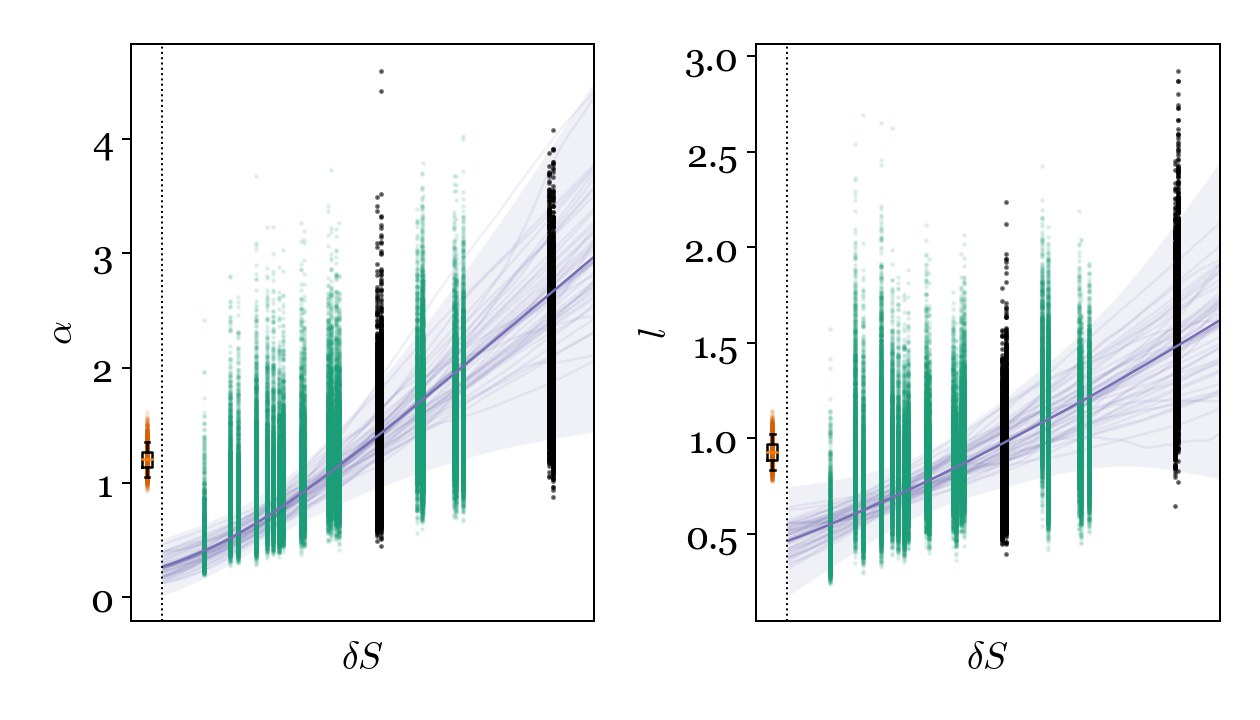
Figure 7: Posterior distributions $p(\boldsymbol{\theta}_{k}\mid\mathbf{y})$ following each method of learning from the series of AE experiments. Independent learners (STL, green); Shared GP prior (MTL A, orange); Hyperparameter modelling (MTL B, purple).

We can see that the (purple) functions $\{g,h\}$ successfully capture the hyperparameter relationships while also reducing the variance when compared to independent models (green) without assuming one consistent hyperparameter (orange). Critically, while all parameters make sense in view of the respective assumptions, the GP model of the hyperparameters (purple) is clearly more expressive: it represents the variations of the map between experiments with respect to an explanatory variable (sensor separation).

Modelling hyperparameters, not parameters

Why not include $\delta S_{k}$ as an explanatory variable on the lower level – within a product kernel, for example? This is because changes in the response itself are not smooth as we vary $\delta S_{k}$ – in fact, the response surface switches quite dramatically between experiments, see Figure 3. Instead, the characteristics of the responses (smoothness, process variance) have smooth relationships with respect to $\delta S_{k}$ (observed in Figures 7 and 6). For this reason, it is more appropriate to model variations at the hyperparameter level, rather than the map itself (as expected with more typical spatiotemporal models, for example).

Post-selection inference

By investigating (independent) model behaviour with plots of the posterior distributions, we use the training data twice: (i) for inference, (ii) to inform model design. Specifically, Figure 6 was used to inform the structure of the multilevel model, so we are guilty of post-selection inference [26]. With reference to Gelman et al. [3], we consider that, when the number of candidate models is small, the bias resulting from data reuse is also small. In our case, the plots informed only certain aspects of the higher-level GP design. Post-selection inference should be treated cautiously, however, as when the number of candidate models grows, the risk of overfitting the data increases.

5 Results and Discussion

To test each method of representing the experimental data, the ground truth (or target) out-of-sample data $\{\mathbf{\bar{y}}_{k}\}_{k=1}^{k}$ are compared to the posterior predictive distribution. The predictive log-likelihood is used as a probabilistic assessment of performance,

$$\textrm{lpY}_{k}=\sum_{i=1}^{N}\log\left(\frac{1}{S}\sum_{s=1}^{S}p\big{(}\bar{y}_{ik}\mid\boldsymbol{\Theta}^{p}_{s}\big{)}\right)$$ (38)

where $\boldsymbol{\Theta}^{p}_{s}$ is a single sample from the full posterior distribution and the combined likelihood of all models is $\textrm{lpY}=\sum_{k=1}^{K}\textrm{lpY}_{k}$. In words, (38) quantifies the (log) likelihood that test data were generated by the model inferred from the training data. A higher value indicates that the model has a better approximation of the underlying data-generating process and indicates good generalisation.

Figure 8 presents lpY for all benchmarks. There is an improvement in the combined predictive likelihood for both MTL methods. For task-specific performance ($\textrm{lpY}_{k}$) independent STL learners perform slightly better for a subset of domains $k\in\{5,8,10,11,13\}$. This is typical, however, since MTL considers the joint distribution of the whole data: if some experiments have better data than others (fewer outliers, less noise) these might lose out, while models with inferior data improve.

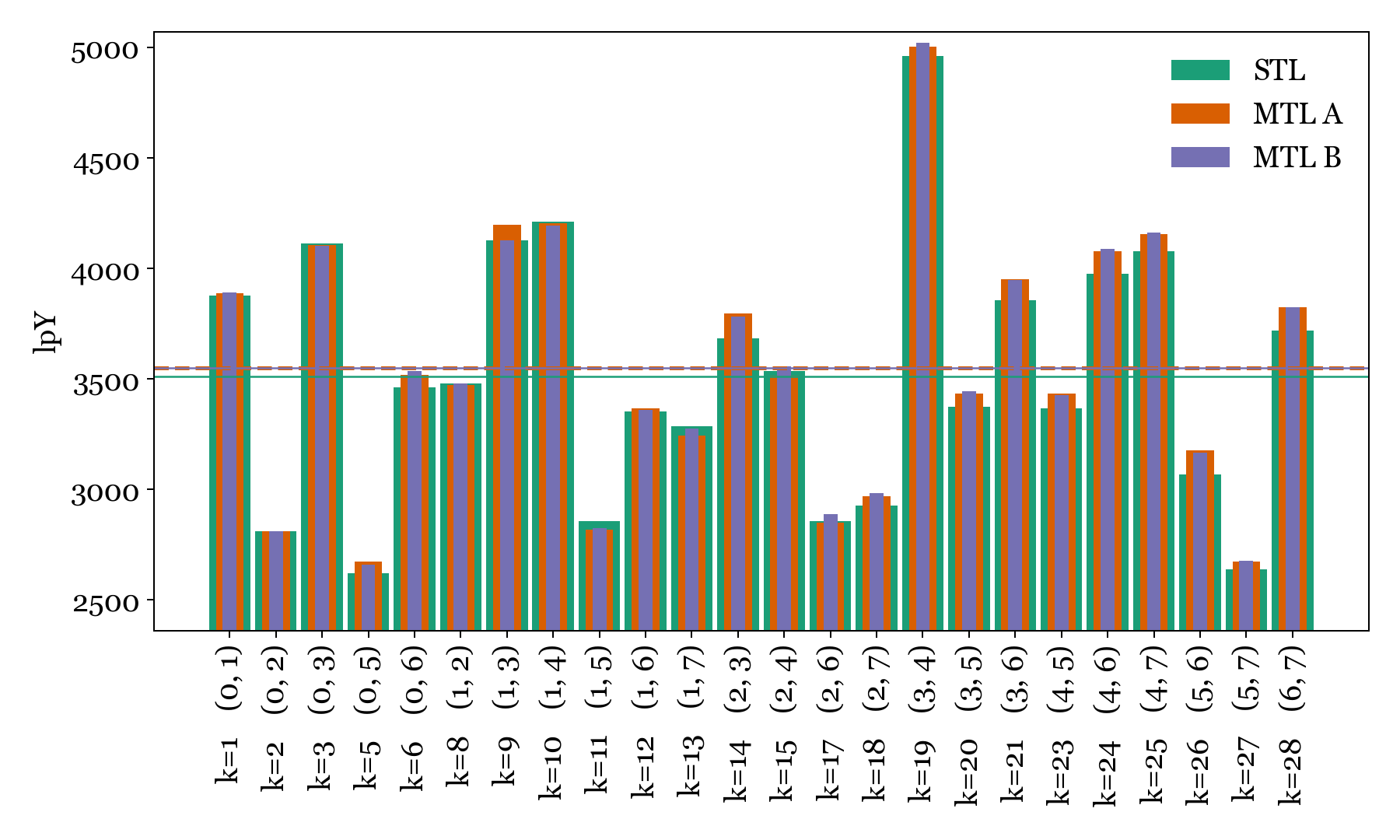
Figure 8: Predictive log-likelihood for the out-of-sample test data. Lines plot the average across all domains, the formal combined log-likelihood (summed) for each method is: (STL, 84217), (MTL A, 85149), (MTL B, 85204).

Both MTL A and B extend data for training by partial pooling, but B has a more descriptive multilevel structure, allowing us to encode domain expertise for intertask (between experiment) learning. In turn, hyperparameter relationships are captured over the experimental campaign (rather than their marginal distribution). By modelling prior variations in MTL B, it represents changes in the tasks with respect to experimental design parameters (in this case $\delta S_{k}$) enabling further insights. To summarise:

• (A & B) can simulate the response for hypothetical/unobserved experimental setups

• (B) has the potential to encode physics/domain expertise of behaviour between sensor pairs (mean functions, constraints)

• (A & B) can use the parameter relationships, learnt from similar experiments, to predict optimal hyperparameters in domains with sparse data (this can be viewed as a form of transfer learning)

5.1 Using the multilevel model for transfer learning

We demonstrate the final point from the list above, to interpolate and extrapolate in the model space. The results intend to show how multilevel models can capture overarching insights from the experimental campaign (at the systems level) as well as task-specific insights. The expected hyperparameter values $\textrm{E}[\boldsymbol{\theta}_{k}]$ from MTL A and B can be visualised in Figure 7 with the solid lines. These point estimates are used when conditioning on data from the hold-out tests. In turn, hyperparameter inference can be avoided for new (previously unobserved) experiments. Instead, we predict their value given the other, similar experiments: where MTL A assumes one hyperparameter set for all tests, and MTL B learns how these vary with respect to sensor separation. By using parameter predictions informed by data-rich training domains, we should improve the predictive performance for sparse data with the new experiments.

To demonstrate, the expected values are used to condition new GPs for an increasing training budget ($N=5\;\textrm{-}\;100$) for the hold-out experiments. Figure 9 shows that both forms of MTL consistently improve the predictive performance, especially when extrapolating in the model space ($\delta S=0.54$). These improvements are intuitive since the extrapolated parameters are associated with higher uncertainty for conventional STL (refer to Figure 7). Another (more natural) way to share information would be to retrain the MTL models to include held-out experiments while increasing the training data. We favour the method presented here for computational reasons, referring again to the footnote¹.

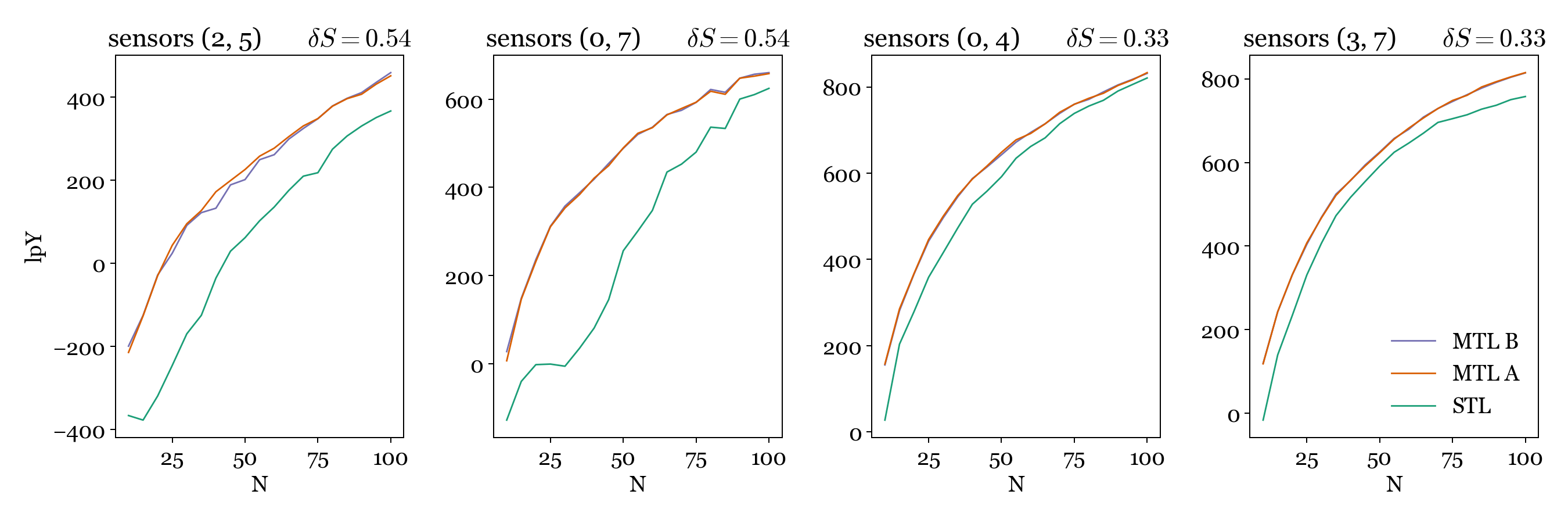
Figure 9: Predictive log-likelihood for an increasing training budget for the hold-out experiments. Conventional single-task learning (STL) compared to multitask learning (MTL) which predicts hyperparameter values from similar experiments. Averaged for 100 repeats.

These results demonstrate a form of transfer learning since the information from the training experiments (source domains) is used to improve prediction for held-out experiments (target domains). However, both MTL A and B provide (effectively) the same performance increase. This raises the question: is the more descriptive model for $p(\boldsymbol{\theta}\mid\phi)$ worth it, given that A provides the same predictive performance? We argue that this depends on the purpose of the model. If the purpose is purely prediction, the assumptions of A will likely be sufficient (in engineering, however, prediction is rarely the only motivation). On the other hand, B more closely resembles our understanding and domain expertise of the experimental campaign: it provides more insights regarding variations of the AE map between each experiment.

6 Concluding Remarks

In this work, we demonstrated how multilevel Gaussian processes can be used to represent aggregate systems in engineering applications. Two model formulations were used to represent a series of experiments concerning source location with acoustic emissions (AE) for a complex plate geometry. While the same plate was used throughout the test campaign, the experimental design was varied (re. sensor placement). By learning all tasks in a joint inference, the representation captures how characteristics of the AE map (i.e. hyperparameters) vary between the experiments. The model can also share information between tasks, to extend the (effective) number of training data and their value. We presented the intertask relations and explained how they inform insights into systems-level behaviour, allowing domain expertise to be encoded between experiments relating to the effects of design variables on the outcome of each test. We used the multilevel model to predict hyperparameter values of similar (previously unobserved) experiments, to enhance inference in new domains by transfer learning.

Looking forward, it would be interesting to encode more specific physics-based constraints into multilevel representations, to describe intertask variations with scientific processes. Instead, this article encoded domain expertise of the underlying physics, such that the data simulated by the hierarchical model reflect our understanding of the environment and experiments.

Appendix

Appendix A A Gaussian identity for GP prediction

Let $\mathbf{x}$ and $\mathbf{y}$ be jointly Gaussian random vectors [27],

$$\left[\begin{array}[]{l}\mathbf{x}\\ \mathbf{y}\end{array}\right]\sim\textrm{N}\left(\left[\begin{array}[]{l}\boldsymbol{\mu}_{x}\\ \boldsymbol{\mu}_{y}\end{array}\right],\left[\begin{array}[]{ll}A&C\\ C^{\top}&B\end{array}\right]\right)=\textrm{N}\left(\left[\begin{array}[]{l}\boldsymbol{\mu}_{x}\\ \boldsymbol{\mu}_{y}\end{array}\right],\left[\begin{array}[]{ll}\tilde{A}&\tilde{C}\\ \tilde{C}^{\top}&\tilde{B}\end{array}\right]^{-1}\right)$$

The conditional distribution of $\mathbf{x}$ given $\mathbf{y}$ is

$$\mathbf{x}\mid\mathbf{y}\sim\textrm{N}\left(\boldsymbol{\mu}_{x}+CB^{-1}\left(\mathbf{y}-\boldsymbol{\mu}_{y}\right),A-CB^{-1}C^{\top}\right)$$

This conditional is used in GP predictive equations, for a given/fixed set (i.e. sample) of hyperparameters. For further details, refer to Rasmussen et al. [27].

References

- Gardner et al. [2022] P. Gardner, L. A. Bull, J. Gosliga, N. Dervilis, E. J. Cross, E. Papatheou, and K. Worden. Population-Based Structural Health Monitoring, pages 413–435. Springer International Publishing, 2022.
- Rahwan et al. [2019] I. Rahwan, M. Cebrian, N. Obradovich, J. Bongard, J.-F. Bonnefon, C. Breazeal, J. W. Crandall, N. A. Christakis, I. D. Couzin, M. O. Jackson, N. R. Jennings, E. Kamar, I. M. Kloumann, H. Larochelle, D. Lazer, R. McElreath, A. Mislove, D. C. Parkes, A. S. Pentland, M. E. Roberts, A. Shariff, J. B. Tenenbaum, and M. Wellman. Machine behaviour. Nature, 568(7753):477–486, 2019.
- Gelman et al. [2013] A. Gelman, J. B. Carlin, H. S. Stern, D. B. Dunson, A. Vehtari, and D. B. Rubin. Bayesian Data Analysis. CRC press, third edition, 2013.
- Bull et al. [2022] L. A. Bull, D. Di Francesco, M. Dhada, O. Steinert, T. Lindgren, A. K. Parlikad, A. B. Duncan, and M. Girolami. Hierarchical bayesian modelling for knowledge transfer across engineering fleets via multitask learning. Computer-Aided Civil and Infrastructure Engineering, 2022.
- Murphy [2012] K. P. Murphy. Machine Learning: A Probabilistic Perspective. MIT press, 2012.
- Hensman et al. [2010] J. Hensman, R. Mills, S. Pierce, K. Worden, and M. Eaton. Locating acoustic emission sources in complex structures using Gaussian processes. Mechanical Systems and Signal Processing, 24(1):211–223, 2010.
- Karniadakis et al. [2021] G. E. Karniadakis, I. G. Kevrekidis, L. Lu, P. Perdikaris, S. Wang, and L. Yang. Physics-informed machine learning. Nature Reviews Physics, 3(6):422–440, 2021.
- Willard et al. [2020] J. Willard, X. Jia, S. Xu, M. Steinbach, and V. Kumar. Integrating physics-based modeling with machine learning: A survey. arXiv preprint arXiv:2003.04919, 1(1):1–34, 2020.
- Daw et al. [2021] A. Daw, A. Karpatne, W. Watkins, J. Read, and V. Kumar. Physics-guided neural networks (pgnn): An application in lake temperature modeling. arXiv, 2021.
- Wahlström et al. [2013] N. Wahlström, M. Kok, T. B. Schön, and F. Gustafsson. Modeling magnetic fields using Gaussian processes. In 2013 IEEE International Conference on Acoustics, Speech and Signal Processing, pages 3522–3526. IEEE, 2013.
- Alvarez et al. [2009] M. Alvarez, D. Luengo, and N. D. Lawrence. Latent force models. In Artificial Intelligence and Statistics, pages 9–16. PMLR, 2009.
- Jones et al. [2023] M. R. Jones, T. J. Rogers, and E. J. Cross. Constraining Gaussian processes for physics-informed acoustic emission mapping. Mechanical Systems and Signal Processing, 188:109984, 2023.
- Huang et al. [2019] Y. Huang, J. L. Beck, and H. Li. Multitask sparse Bayesian learning with applications in structural health monitoring. Computer-Aided Civil and Infrastructure Engineering, 34(9):732–754, 2019.
- Huang and Beck [2015] Y. Huang and J. L. Beck. Hierarchical sparse Bayesian learning for strucutral health monitoring with incomplete modal data. International Journal for Uncertainty Quantification, 5(2), 2015.
- Di Francesco et al. [2021] D. Di Francesco, M. Chryssanthopoulos, M. H. Faber, and U. Bharadwaj. Decision-theoretic inspection planning using imperfect and incomplete data. Data-Centric Engineering, 2, 2021.
- Papadimas and Dodwell [2021] N. Papadimas and T. Dodwell. A hierarchical Bayesian approach for calibration of stochastic material models. Data-Centric Engineering, 2, 2021.
- Hughes et al. [2023] A. J. Hughes, P. Gardner, and K. Worden. Towards risk-informed pbshm: Populations as hierarchical systems. arXiv preprint arXiv:2303.13533, 2023.
- Sedehi et al. [2023] O. Sedehi, A. M. Kosikova, C. Papadimitriou, and L. S. Katafygiotis. On the integration of physics-based machine learning with hierarchical bayesian modeling techniques. arXiv preprint arXiv:2303.00187, 2023.
- Shull [2002] P. J. Shull. Nondestructive evaluation: theory, techniques, and applications. CRC press, 2002.
- Tobias [1976] A. Tobias. Acoustic-emission source location in two dimensions by an array of three sensors. Non-destructive testing, 9(1):9–12, 1976.
- Jones et al. [2022a] M. R. Jones, T. J. Rogers, K. Worden, and E. J. Cross. A bayesian methodology for localising acoustic emission sources in complex structures. Mechanical Systems and Signal Processing, 163:108143, 2022a.
- Jones et al. [2022b] M. R. Jones, T. J. Rogers, K. Worden, and E. J. Cross. Heteroscedastic Gaussian processes for localising acoustic emission. In Data Science in Engineering, Volume 9: Proceedings of the 39th IMAC, A Conference and Exposition on Structural Dynamics 2021, pages 185–197. Springer, 2022b.
- Hoffman et al. [2014] M. D. Hoffman, A. Gelman, et al. The no-u-turn sampler: adaptively setting path lengths in hamiltonian monte carlo. J. Mach. Learn. Res., 15(1):1593–1623, 2014.
- Carpenter et al. [2017] B. Carpenter, A. Gelman, M. D. Hoffman, D. Lee, B. Goodrich, M. Betancourt, M. Brubaker, J. Guo, P. Li, and A. Riddell. Stan: A probabilistic programming language. Journal of statistical software, 76(1), 2017.
- Wiemann et al. [2021] P. F. Wiemann, T. Kneib, and J. Hambuckers. Using the softplus function to construct alternative link functions in generalized linear models and beyond. arXiv preprint arXiv:2111.14207, 2021.
- Lee et al. [2016] J. D. Lee, D. L. Sun, Y. Sun, and J. E. Taylor. Exact post-selection inference, with application to the lasso. The Annals of Statistics, pages 907–927, 2016.
- Rasmussen et al. [2006] C. E. Rasmussen, C. K. Williams, et al. Gaussian Processes for Machine Learning, volume 1. Springer, 2006.