Dynamics of the clumps partially disrupted from a planet around a neutron star

Abstract

Tidal disruption events are common in the Universe, which may occur in various compact star systems and could account for many astrophysical phenomena. Depending on the separation between the central compact star and its companion, either a full disruption or a partial disruption may occur. The partial disruption of a rocky planet around a neutron star can produce kilometer-sized clumps, but the main portion of the planet can survive. The dynamical evolution of these clumps is still poorly understood. In this study, the characteristics of partial disruption of a rocky planet in a highly elliptical orbit around a neutron star is investigated. The periastron of the planet is assumed to be very close to the neutron star so that it would be partially disrupted by tidal force every time it passes through the periastron. It is found that the fragments generated in the process will change their orbits on a time scale of a few orbital periods due to the combined influence of the neutron star and the remnant planet, and will finally collide with the central neutron star. Possible outcomes of the collisions are discussed.

1 Introduction

Tidal disruption happens when an object gets too close to its compact host. Tidal disruption associated with black holes (BHs) has been extensively studied (see Guillochon & Ramirez-Ruiz (2013), Ryu et al. (2020), Gezari (2021) Mageshwaran & Mangalam (2021), Rossi et al. (2021) and references therein). For the disruption of planetary objects, pioneer works have been done by Faber et al. (2005), Guillochon et al. (2011), and Liu et al. (2013) on gas giants. Especially, Faber et al. (2005) and Liu et al. (2013) simulated the single tidal encounter of a close gas giant, whereas the cases of multiple passage encounters were studied in Guillochon et al. (2011) and Veras et al. (2014).

Tidal disruption of minor-planets/asteroids around white dwarfs (WDs) has been extensively studied (Vanderburg et al., 2015; Granvik et al., 2016). Recent simulations (Malamud & Perets, 2020a, b) show that a planet in a highly eccentric orbit around a WD could be disrupted by tidal force, and materials in the inner side of the orbit would be accreted by the WD. The material accreted by the WD may be responsible for the pollution of the WD atmosphere by heavy elements (Vanderburg et al., 2015; Malamud & Perets, 2020a, b). Similar processes can also occur in neutron star-planet systems if the initial parameters of the planetary system fulfill the tidal disruption condition (Geng et al., 2015; Huang & Yu, 2017; Kuerban et al., 2019; Kuerban et al., 2020; Kurban et al., 2022).

Depending on the relative separation between the compact star and the companion object, the degree of disruption could be very different. Either a full disruption or a partial disruption may occur. In full disruption, the companion is completely destroyed. In this case, the time for the debris material to be completely accreted by the compact star could be very long especially when no additional forces connected to sublimation or radiation are involved (Veras et al., 2014). In the case of a partial disruption, part of the material is stripped off from the orbiting object. For example, the partial disruption of a rocky planet can produce kilometer-sized clumps, but the main portion of the planet can still survive (Malamud & Perets, 2020a). The fate of clumps is then affected by the combined action of the surviving planet and the compact star, the studying of which is still lacking in the literature.

Most of the previous studies mainly focus on the tidal disruption of an object in a parabolic or elliptic orbit. Formation of such an orbit is considered to be the results of various dynamical processes such as tidal capturing (Goulinski & Ribak, 2018; Kremer et al., 2019), Kozai-Lidov effect (Lidov, 1962; Kozai, 1962; Naoz, 2016; Shevchenko, 2017), or scattering (Hong et al., 2018; Carrera et al., 2019). The planet may have multiple close encounters with the central star in a tidal capturing process. In the Kozai-Lidov effect, the planet can move close to its central star and multiple encounters could occur naturally due to eccentricity oscillation. The close approach is gradual in this process, and partial disruption may occur. In addition, the probability of partial disruption is usually higher than that of full disruption (Zhong et al., 2022). The investigation of the dynamic behavior of the clumps produced in a partial disruption is important, which could help understand various astrophysical phenomena such as electromagnetic transient events and the pollution of the WD atmosphere by heavy elements.

The Kozai-Lidov mechanism (Lidov, 1962; Kozai, 1962) is an efficient theory to model gravitational interactions in multi-body systems. The interaction in such systems is complicated, and the evolution could be rapid, although no dissipation is involved. Merger events could be triggered and various bursts or transients may be produced in these multi-body systems (Naoz, 2016; Shevchenko, 2017).

In standard Kozai-Lidov theory (Lidov, 1962; Kozai, 1962), the angular momentum of the test particle is conserved when a circular orbit is assumed for the outer perturber, causing periodic variation of the test particle’s eccentricity and inclination. However, the angular momentum for both inner and outer orbits are not conserved when the perturber’s orbit is eccentric, which leads to very different behaviors of the test particle (Lithwick & Naoz, 2011; Li et al., 2014a; Naoz et al., 2017).

In a three-body system, the orbit parameters significantly influence the dynamic outcome. The hierarchy of such a system is mainly determined by the parameter $\epsilon=a_{1}e_{2}/[a_{2}(1-e_{2}^{2})]$ (the coefficient of the octupole-order secular interaction term), or by the factor $a_{2}(1-e_{2})/a_{1}$, both of which parameterize the size of the external orbit as compared to the inner binary orbit. Note that $e$ is the eccentricity and $a$ is the semi-major axis of the inner and outer orbits, denoted by subscripts 1 and 2 respectively. A system with $\epsilon<0.1$ is hierarchical and stable. It is mildly hierarchical when $0.1<\epsilon<0.3$, and is non-hierarchial when $\epsilon>0.3$ (Naoz, 2016). Equivalently, when the factor of $a_{2}(1-e_{2})/a_{1}$ is concerned, a system with $a_{2}(1-e_{2})/a_{1}>10$ is hierarchical. It is moderately hierarchical when $a_{2}(1-e_{2})/a_{1}=$ 3—10, and it is non-hierarchial when $a_{2}(1-e_{2})/a_{1}<3$ (e.g. Antonini & Perets, 2012; Katz & Dong, 2012; Antonini et al., 2014; He & Petrovich, 2018). It has been shown that the orbit-averaging method (including quadrupole and octupole terms) is broken down in non-hierarchial, dynamically unstable systems, and this leads to an underestimation of the maximum eccentricity (Antonini & Perets, 2012; Katz & Dong, 2012; Antonini et al., 2014; He & Petrovich, 2018; Grishin et al., 2018; Bhaskar et al., 2021). It was also found that a system with $a_{2}(1-e_{2})/a_{1}<10$ follows a complex dynamical evolution pattern that can lead to a very large eccentricity and secular approximations can not accurately describe the evolution features.

The hierarchical triple systems in test particle limit have been studied for different scientific cases (Lithwick & Naoz, 2011; Katz et al., 2011; Naoz et al., 2013; Li et al., 2014a, b; Li & Adams, 2016; Li et al., 2018). For a system with nearly coplanar (the inclination $i\sim 0$) and highly eccentric (for both inner and outer orbits) configuration, Li et al. (2014a) found that the eccentricity of the inner test particle increases steadily due to the perturbation (this effect is significant for tight configurations). Recently, Grishin et al. (2018) and Bhaskar et al. (2021) studied the dynamic evolution of highly inclined, mildly hierarchical systems and found that the orbit-average method can describe the evolution of the inner orbit well when $e_{2}=0$. But Bhaskar et al. (2021) found that the orbit-average method is not accurate enough for systems with $a_{1}/a_{2}>0.3$ and $m_{2}/M<6\times 10^{-3}$ (here $M$ is the central star mass), and the accuracy is worsening with the increase of $a_{1}/a_{2}$ (i.e. for a tighter configuration) and the decrease of $m_{2}/M$. Thus the value of $a_{2}(1-e_{2})/a_{1}$ can effectively reflect the stability of the system. If the configuration of the system does not satisfy the stability condition (Mardling & Aarseth, 2001; He & Petrovich, 2018) or the secular approximation of the Kozai-Lidov mechanism is broken-down (Antonini & Perets, 2012; Antonini et al., 2014, 2016), the orbit of the test particle will evolve even faster, essentially causing a collision or ejection.

The goal of this study is to investigate the dynamical evolution of the clumps produced during the partial disruption of a rocky planet that moves around a neutron star (NS) in a highly elliptical orbit. The motion of these clumps is affected by both the NS and the planet’s surviving core, making the system an ideal case for the Kozai-Lidov mechanism. The structure of our paper is as follows. In Section 2, the structure of the planet is described, which is an important factor that affects the dynamics of the clumps. The tidal disruption process is introduced in Section 3, paying special attention on the effects of various parameters. Section 4 presents the distributions of orbital parameters for the clumps. The dynamics of the clumps are detailedly investigated in Section 5, and possible factors that can affect the dynamics are then described in Section 6. Finally, Section 7 presents our conclusions and some brief discussion.

2 The structure of planet

Up to now, more than 5000 exoplanets have been detected. Their measured parameters (mass, radius) indicate that their composition should be different from each other. Various equations of states (EOSs) are proposed for exoplanets (Benz & Asphaug, 1999; Seager et al., 2007; Swift et al., 2012; Howe et al., 2014; Smith et al., 2018; Otegi et al., 2020). In this study, we mainly focus on rocky planets which orbit around neutron stars. Three types of planets will be considered, i.e. pure iron (Fe) planets, pure perovskite (MgSiO₃) planets, and the two-layer planets composed of a Fe core and a MgSiO₃ mantle. For Fe materials, we use the EOS derived based on experimental data, as described in Smith et al. (2018), which is expressed as

$$P_{\rm SM}=3K_{0}x^{-2}\left(1-x\right)\exp\left[\left(1.5K^{\prime}_{0}-1.5\right)\left(1-x\right)\right],$$ (1)

where $x=(\rho_{0}/\rho)^{1/3}$, $\rho_{\rm 0}=8.43\rm\,g\,cm^{-3}$ (the density at zero pressure), $K_{0}=177.7\rm\,GPa$ and $K^{\prime}_{0}=5.64$. For MgSiO₃ materials, we take the third-order finite strain Birch-Murnagham EOS that is widely used for exoplanet modeling (Birch, 1947; Seager et al., 2007), i.e.

$$P_{\rm BM}=\frac{3}{2}K_{0}\left(y^{7/3}-y^{5/3}\right)\left[1+\frac{3}{4}\left(K^{\prime}_{0}-4\right)\left(y^{2/3}-1\right)\right],$$ (2)

where $y=(\rho_{0}/\rho)^{-1}$. In this case, the density at zero pressure is $\rho_{\rm 0}=3.22\rm\,g\,cm^{-3}$, and the two constants are $K_{0}=125\rm\,GPa$ and $K^{\prime}_{0}=5$, respectively.

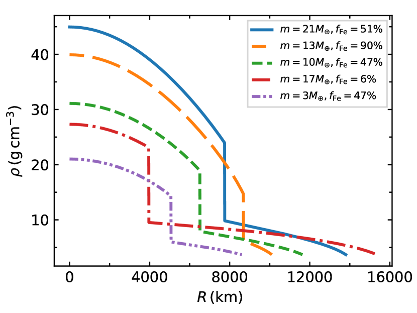
Figure 1: $\rho$ vs. $R$ for two-layer rocky planets with different Fe core mass fraction $f_{\rm Fe}$. The EOS of Smith et al. (2018) is used for the Fe core and the EOS of Seager et al. (2007) is used for the MgSiO₃ mantle (see main text for details). For similar plots, see Seager et al. (2007) and Howe et al. (2014).

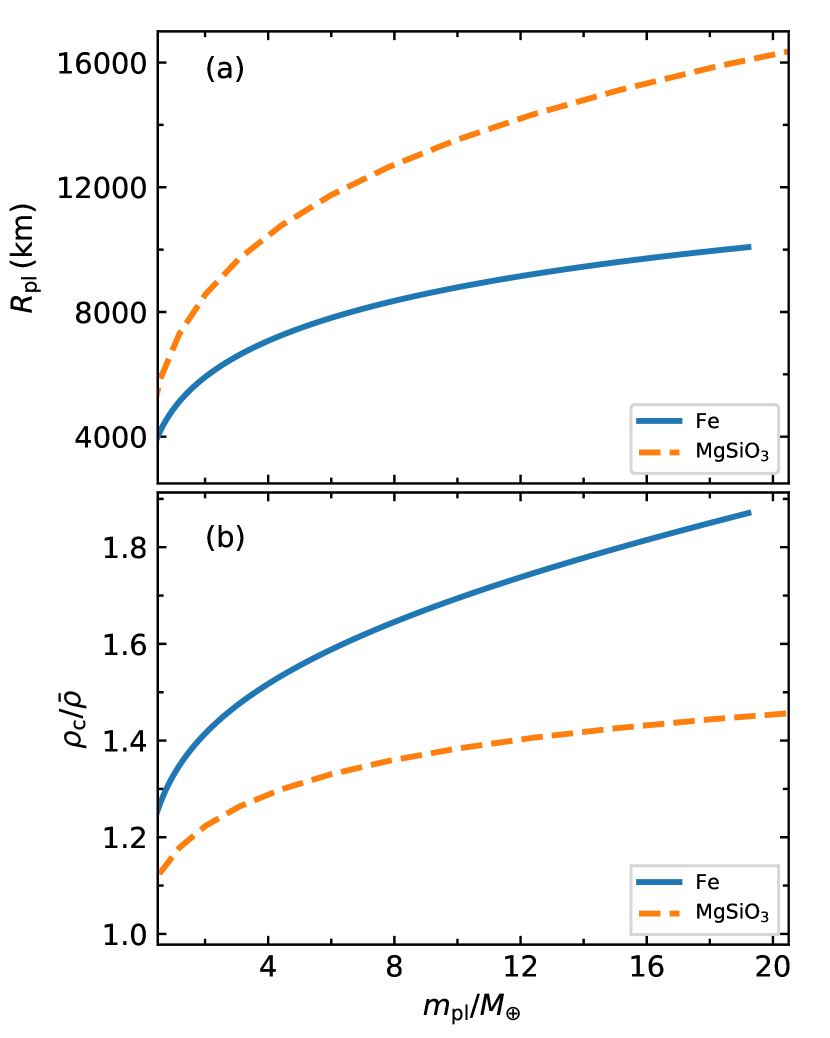
Figure 2: (a) Mass-Radius relation and (b) $\rho_{\rm c}/\bar{\rho}$ vs. mass for pure Fe planets and pure MgSiO₃ planets. For similar plots, see Smith et al. (2018) and Seager et al. (2007).

The mass, radius, and internal density profile of a planet can be calculated by using the above EOSs. The property of a planet composed of pure materials is mainly characterized by its central pressure ($P_{\rm c}$). But for a two-layer planet composed of a Fe core and a MgSiO₃ mantle, both the central pressure and the pressure at the core-mantle boundary ($P_{\rm cb}$) are necessary to determine the mass and radius of the planet. In our calculations, we will take various possible $P_{\rm c}$ and $P_{\rm cb}$ values (Seager et al., 2007; Howe et al., 2014) to study their effects on the dynamics. For a two-layer planet, the EOS can be generally expressed as

$$P=\left\{\begin{array}[]{lr}P_{\rm SM},~{}~{}~{}~{}P\geq P_{\rm cb}~{}~{}~{}~{}(\rm for~{}core)\\ P_{\rm BM}.~{}~{}~{}~{}P<P_{\rm cb}~{}~{}~{}~{}(\rm for~{}mantle)\end{array}\right.$$ (3)

As an example, Fig. 1 plots the $\rho-R$ (density vs. radius) profile of some two-layer planets. Note that the $P_{\rm c}$ and $P_{\rm cb}$ are different for these objects. On each curve, the vertical segment represents the boundary between the core and the mantle, at which there is a jump in density but the pressure is still continuous, that is $P_{\rm cb}$. The mass-radius ($m_{\rm pl}-R_{\rm pl}$) relation of pure Fe planets and pure MgSiO₃ planets is shown in Panel (a) of Fig. 2, and the relation between $m_{\rm pl}$ and $\rho_{\rm c}/\bar{\rho}$ (the ratio of the central density to the mean density) is shown in Panel (b). It can be seen that planets consisting of pure Fe are more compact than those composed of MgSiO₃.

3 Condition of tidal disruption

Let us consider the tidal disruption of a rocky planet by its host, an NS. The planet moves around the NS in an eccentric orbit. The mass of the NS is designated as $M_{\star}$ (in the calculations throughout this paper, we take $M_{\star}=1.4M_{\sun}$), and the planet is a rocky object with a mass of $m_{\rm pl}$ and an orbital period of $P_{\rm orb}$. According to the Kepler’s third law, the semi-major axis ($a$) of the orbit is related to $P_{\rm orb}$ as

$$\frac{P_{\rm orb}^{2}}{a^{3}}=\frac{4\pi^{2}}{G(M_{\star}+m_{\rm pl})}.$$ (4)

The separation between the planet and the central star in an eccentric orbit is phase-dependent. At phase $\theta$, it is $r=a(1-e^{2})/(1+e\,\cos\theta)$, where $e$ is the eccentricity of the orbit. Note that the periastron is $r_{\rm p}=a(1-e)$ in this case.

If the planet is too close to the NS, the central star’s tidal force would exceed the planet’s self-gravity at the surface so that the planet will be disrupted by the tidal force. The critical separation is defined as the tidal disruption radius (Hills, 1975). For a gravity-dominated object, the tidal disruption radius can be expressed as

$$r_{\rm td}=R_{\rm pl}\left(\frac{2M_{\star}}{m_{\rm pl}}\right)^{1/3}.$$ (5)

For a rocky planet, the tidal disruption radius is $r_{\rm td}\sim 10^{11}$ cm. On the other hand, when the distance of the planet is only slightly larger than $r_{\rm td}$, it will also be affected by the tidal force and could be partially disrupted. Fragments of several kilometers in size will be produced during this process. The degree of partial disruption depends on the separation ($r$). The details relevant to partial disruption will be discussed in the next section.

Small bodies with a radius of less than a few kilometers are bounded by material-strength. For them, the intrinsic material shear and cohesive strengths can help resist the tidal force (Sridhar & Tremaine, 1992; Holsapple & Michel, 2008; Zhang & Lin, 2020). According to the elastic-plastic continuum theory (Holsapple & Michel, 2008), the tidal disruption limit of small bodies in the the material-strength dominated regime is (Zhang & Lin, 2020; Zhang et al., 2021)

$$r_{\rm str}=\left(\frac{\sqrt{3}M_{\star}}{4\pi\rho_{\rm cl}}\right)^{1/3}\left(\frac{5k}{4G\pi\rho_{\rm cl}^{2}r_{\rm cl}^{2}}+s\right)^{-1/3},$$ (6)

where $r_{\rm cl}$ and $\rho_{\rm cl}$ are the radius and density of the small body (clump), respectively. The two constants $s$ and $k$ can be expressed as a function of the friction angle $\phi$ and the cohesive strength $C$, $s=2\sin\phi/\sqrt{3}(3-\sin\phi)$ and $k=6C\cos\phi/\sqrt{3}(3-\sin\phi)$. The friction angle usually ranges in $25^{\circ}$ — $50^{\circ}$ (Holsapple & Michel, 2008; Bareither et al., 2008). The cohesive strength of meteorites/asteroids is typically in the range of 0.1-10 MPa (Pohl & Britt, 2020; Veras & Scheeres, 2020), while it is $\sim$1 Pa for comets (Gundlach & Blum, 2016). In our case, the small clump typically has a size of 2 km and a density of $\rho_{\rm cl}=5\,\rm g\,cm^{-3}$ (typical density for MgSiO₃). Taking $\phi=30^{\circ}$, then the break up distance is $r_{\rm str}=5.31\times 10^{10}$ cm for $C$ = 0.1 MPa, and it is $r_{\rm str}=9.88\times 10^{9}$ cm for $C$ = 10 MPa. Alternatively, taking $\phi=45^{\circ}$, we have $r_{\rm str}=2.41\times 10^{10}$ cm for $C$ = 0.1 MPa, and $r_{\rm str}=5.34\times 10^{9}$ cm for $C$ = 10 MPa. It means that the small body will remain intact even when they are very close to the central star.

4 Orbits of the clumps

In this study, we consider a rocky planet moving around an NS in a highly elliptical orbit. The periastron is assumed to be slightly larger than the tidal disruption radius so that the planet will be partially disrupted every time it passes through the periastron. A few clumps of several kilometers are generated in the process. The condition of the NS-planet system determines the features of the stripped clumps. First, the degree of disruption is determined by the ratio of the tidal disruption radius with respect to the periastron, which we define as the penetration factor ($\beta$), i.e. $\beta=r_{\rm td}/r_{\rm p}$. If $\beta$ is large (the separation is small at the periastron), then the disruption is violent and the planet would be significantly destroyed. On the other hand, when $\beta$ is small (the separation is large), the planet will only be lightly affected. The material in the outer crust of the planet will be stripped off to produce some rocky clumps, but the planet itself will largely remain its integrity (e.g. Manser et al., 2019; Guillochon et al., 2011; Liu et al., 2013; Malamud & Perets, 2020a, b; Law-Smith et al., 2020).

The mass stripped from the planet depends on its structure and the penetration factor ($\beta$). The mass loss ($\Delta m$) is very small when $\beta\lesssim 0.5$ (Guillochon et al., 2011; Liu et al., 2013; Ryu et al., 2020; Law-Smith et al., 2020). It corresponds to a periastron separation of $r_{\rm p}\gtrsim 2r_{\rm td}$. Here we take $r_{\rm p}=2r_{\rm td}$ as a typical condition for partial disruption, which is used to determine the orbit parameters of the planet and the clumps in the following calculations.

After disruption, the clumps are still bound to the central star, but they should have slightly different orbital parameters since they originate from different parts of the planet. It is very similar to the disruption of a planet around a WD (Malamud & Perets, 2020a, b; Brouwers et al., 2022, 2023). For example, the semi-major axis ($a_{\rm cl}$) of the clump orbit depends on the $\beta$ and displacement ($R$) of the clump relative to the mass center of the planet at the moment of breakup ($R=0$ corresponds to the center of the planet). As a result, the semi-major axis of a clump stripped off from the inner and outer side of the planet is (Malamud & Perets, 2020a)

$$a_{\rm cl}=\left\{\begin{array}[]{lr}a\left(1+a\frac{2R}{d(d-R)}\right)^{-1},~{}~{}(\rm inner)\\ a\left(1-a\frac{2R}{d(d+R)}\right)^{-1},~{}~{}(\rm outer)\end{array}\right.$$ (7)

where $d$ is the distance between the NS and the planet at the moment of break up (here $d=r_{\rm p}$).

According to Kepler’s third law, the orbit period of the clump is

$$P_{\rm orb}^{\rm cl}=\left(\frac{4\pi^{2}a_{\rm cl}^{3}}{G(M_{\star}+m_{\rm cl})}\right)^{1/2}.$$ (8)

As the clump returns to the periastron of its orbit, one has $r_{\rm p}=a_{\rm cl}(1-e_{\rm cl})\pm R$ (here $+$ and $-$ for inner and outer clumps), and the eccentricity is

$$e_{\rm cl}=\left\{\begin{array}[]{lr}1-\frac{r_{\rm p}-R}{a_{\rm cl}},~{}~{}(\rm inner)\\ 1-\frac{r_{\rm p}+R}{a_{\rm cl}},~{}~{}(\rm outer)\end{array}\right.$$ (9)

The spread of orbital parameters of clumps is determined by their original locations on the planet ($R$, inside the planet), and by the $\beta$ parameter. Different $\beta$ leads to different outcomes, such as a full disruption or a partial disruption. In this study, as explained above, we mainly consider the partial disruption cases, for which we take a typical condition of $\beta=0.5$ (or $d=r_{\rm p}=2r_{\rm td}$). The clumps are assumed to originate from the planet’s surface ($R\sim R_{\rm pl}$), while the main portion of the planet remains unaffected. As a result, the orbital parameters of the clumps, such as $a_{\rm cl}$ and $e_{\rm cl}$, will be slightly different from that of the original planet. For example, if we take $P_{\rm orb}=100$ day, $m_{\rm pl}=12.84\,M_{\oplus}$, $R_{\rm pl}=10107.08$ km for a two-layer planet, and assume that materials with $\Delta R=200$ km in depth are stripped off from the surface to form clumps, i.e $R=[R_{\rm pl}-\Delta R,R_{\rm pl}]$, then the eccentricity of the resultant clumps will be in a narrow range of $e_{\rm cl}=[0.96469,0.96422]$. We see that for two clumps originated from $R=R_{\rm pl}-\Delta R$ and from $R_{\rm pl}$, their difference in the orbital eccentricity is very small. Therefore, we only need to consider the case of the clumps in the innermost orbit.

We now further estimate the orbit parameters of our systems under the partial disruption condition. Taking the planet’s orbit period as $P_{\rm orb}=10$ days, $100$ days, and $1000$ days, respectively, we have calculated the parameters of the planet and the clumps. They are plotted versus the planet mass in Fig. 3, some exemplar parameters are presented in Table 1. Here, the left panels show the cases for Fe planets and the right panels show the cases for MgSiO₃ planets. We see that the planet’s eccentricity increases while the semi-major axis and eccentricity of the clumps decrease as the planet’s mass increases. At the same time, to acquire a long orbital period, the semi-major axis and eccentricity of the planet should be large enough. This is easy to understand. The dependence of $a_{\rm cl}$ and $e_{\rm cl}$ on the two parameters of $m_{\rm pl}$ and $R_{\rm pl}$ is expressed in Equations (7) and (9). Note that in these two equations, we have $d=r_{\rm p}=2r_{\rm td}$. From Equation (7), we see that $a_{\rm cl}$ is mainly determined by $R$ and $r_{\rm td}$, but is almost independent on $m_{\rm pl}$ since $m_{\rm pl}\ll M_{\star}$. The dependence of $e_{\rm cl}$ on $m_{\rm pl}$ and $R_{\rm pl}$ is similar.

Whether the clumps are bound to the NS or not is an important issue concerning the tidal disruption process. Clumps in the inner stream with $a_{\rm cl}<a$ are bound to NS. However, for the clumps with $a_{\rm cl}>a$ in the outer stream, we need to consider a critical displacement of $R_{\rm crit}=d^{2}/(2a-d)$ on the far side of the NS (e.g. Malamud & Perets, 2020a). The clumps coming from $R<R_{\rm crit}$ are bound while the clumps with $R>R_{\rm crit}$ form parabolic orbits and are finally unbound to the NS. We will further investigate this issue in the next section.

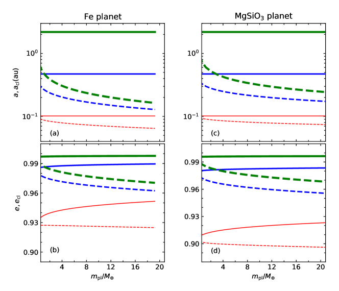
Figure 3: Panel (a) shows the planet’s semi-major axis (solid lines) and the clump’s semi-major axis (dashed lines) as a function of the planet’s mass. The red, blue, and green lines represent the planet with an orbital period of 10 days, 100 days, and 1000 days, respectively. Panel (b) shows the planet’s eccentricity (solid lines) and clump’s eccentricity (dashed lines) as a function of the planet’s mass. The line colors are the same as in Panel (a). The right panels (c) and (d) show the cases for MgSiO₃ planets, and the line styles are the same as that in the left panels.

The inclination angle ($i$) of the clump is determined by its vertical position at the surface of the planet. The maximum inclination is $i=arc\,\,tan(R_{\rm pl}/r_{\rm td})$. But in typical cases, we can assume that the clump originates from a vertical height of $R_{\rm pl}/2$, then the inclination is $i=arc\,\,tan(R_{\rm pl}/2r_{\rm p})$. For example, for a 10$M_{\oplus}$ Fe planet, the inclination is $i=0.2^{\circ}$, while for a 18$M_{\oplus}$ Fe planet, it is $i=0.24^{\circ}$. We see that the inclination is generally very small so that the clumps are essentially coplanar with the planet. Note that the rotation of the planet is also an important factor that can influence the inclination of the clumps. If the planet’s rotation axis is misaligned with its orbital rotation axis, then the inclination could be slightly larger.

5 Dynamics of the clumps

In the above section, we have presented the condition of partial disruption for a rocky planet around an NS. The clumps generated during the partial disruption will orbit around the NS under the influence of gravitational perturbation of the surviving portion of the planet. As a result, the orbit of each clump will evolve and the eccentricity would increase, which will finally make the clumps fall toward the NS. In this section, we present details of the dynamics.

After disruption, the NS, the surviving portion of the planet and the clumps form a multi-body system. Ignoring the interaction between clumps, the system can be simplified as a triple system, which includes the NS, the remnant planet, and a particular clump. The stability of a triple system has been studied for a long time (Eggleton & Kiseleva, 1995; Mardling & Aarseth, 2001). Recently, He & Petrovich (2018) introduced a stability criterion for triple systems, which can be expressed as

$$\frac{a\left(1-e\right)}{a_{\rm cl}\left(1+e_{\rm cl}\right)}>2.8\frac{1}{1+e_{\rm cl}}$$

$$\times\left[\left(1+\frac{m_{\rm pl}}{M_{\star}+m_{\rm cl}}\right)\frac{1+e}{(1-e)^{1/2}}\right]^{2/5}\left(1-\frac{0.3i}{180^{\circ}}\right),$$ (10)

where $e$ and $a$ are the orbital parameters of the planet, $e_{\rm cl}$ and $a_{\rm cl}$ are the parameters of the clump. Note that this criterion applies to any triple system. If a system satisfies the above criteria, then it is stable. On the contrary, if the system does not satisfy the above criteria, then the secular evolution approximation underlying the Kozai-Lidov theory will break down. In such an unstable system, the clump will either be ejected or collide with the central object.

Besides, there is another instability that can make the orbit unstable, in which the secular approximation is breakdown (Antonini & Perets, 2012; Antonini et al., 2014, 2016; Hamers, 2018; Hamers et al., 2022). In this case, the evolutionary timescale of the clump’s angular momentum is comparable to the orbital period of the planet. Several methods have been proposed to deal with the breakdown of the secular approximation, including quadrupole approximation or even higher order contribution (Naoz et al., 2011; Katz & Dong, 2012; Seto, 2013; Naoz et al., 2013), or the double-averaging approaching (Katz & Dong, 2012; Antonini et al., 2014, 2016; Bode & Wegg, 2014). It is found that the orbit of the clump can have a high eccentricity irrespective of its initial inclination. As a result, the clump will finally collide with the central star (e.g. Perets & Kratter, 2012; Katz & Dong, 2012; Bode & Wegg, 2014; Petrovich, 2015; He & Petrovich, 2018; Toonen et al., 2022).

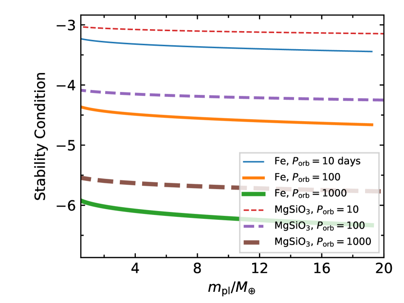
Figure 4: Stability condition for the system composed of the NS, the surviving portion of the planet, and the clump. The solid and dashed lines represent Fe and MgSiO₃ planets with different orbital periods, respectively. A stability condition smaller than zero means that the system is unstable.

We have assessed the stability of the clump’s orbit by using equation (5). The results are plotted in Fig. 4. Note that the stability condition is calculated by subtracting the right-hand side from the left-hand side of Equation (5). It could be seen that, in our cases, the stability condition for all configurations is smaller than zero, meaning that the orbits of the clumps are unstable. As stated above, such unstable clumps will either be ejected from the system or collide with the NS. If the separation ($r$) between the NS and clump is larger than a critical separation of $5a$, the clump will essentially become free (e.g. He & Petrovich, 2018). We have checked the fate of the clumps by using this method. Since the NS has a strong magnetic field, the clumps can be magnetically captured by the NS when they approach the magnetosphere (Geng et al., 2020). As a result, the periastron distance of the clump’s orbit should be larger than the magnetosphere radius, which is roughly $d_{\rm c}\sim 10^{9}$ cm. Correspondingly, the critical eccentricity should be $e_{\rm c}=1-d_{\rm c}/a_{\rm cl}$, and the apocenter distance (the largest separation between the NS and the clump on the orbit) is $r_{\rm a,c}=a_{\rm cl}(1+e_{\rm c})$. We then can compare $r_{\rm a,c}$ with $5a$ to judge the fate of the clumps. To do so, let us define $C_{\rm eje}=r_{\rm a,c}-5a$. If $C_{\rm eje}>0$, the clump will be ejected. Using this approach, we have checked our cases and plotted the results in Panel (a) of Fig. 5. It could be seen that none of the clumps in the inner orbit will be ejected. This result is reasonable. The parent object of the clumps, i.e. the planet itself, is a bound object in our framework. So, the clumps will also be bound. On the other hand, if the planet is a free object which happens to pass by the NS, then the disrupted clumps would mainly be unbound and would be ejected.

On the other hand, it has been argued that the torque exerted by the outer perturber on the clump is large enough to lead the clumps to collide with the NS in one orbit period if the condition

$$C_{\rm col}=2.55\left(\frac{a_{\rm cl}}{2d_{\rm c}}\right)^{1/6}\left(\frac{m_{\rm pl}}{M_{\star}+m_{\rm cl}}\right)^{1/3}-\frac{a\left(1-e\right)}{a_{\rm cl}}>0$$ (11)

is satisfied (e.g. He & Petrovich, 2018). Using this criterion, we have checked the clumps in the system and plotted the results in Panel (b) of Fig. 5. From this figure, we could further see that $a(1-e)/a_{\rm cl}<0.12$ and $\epsilon>0.3$ are satisfied in all the cases, indicating that they are non-hierarchical and unstable so that the secular approximation is broken down.

In short, our system satisfies the collision condition. This is due to the fact that the action of the surviving planet can significantly change the clump’s angular momentum at periapsis (e.g. Antonini et al., 2014; Zhang et al., 2023), leading to a quick reduction of the pericenter separation so that a head-on collision will finally occur. During the process, the closeness of the clump’s orbit with respect to that of the surviving planet, together with the asymmetric configuration (i.e. the eccentric orbit of the planet), is the key factor that takes effect. Note that the perturbation effect of the planet is strong in less hierarchical and dynamically unstable systems (e.g. Toonen et al., 2022). Below, we will calculate the evolutionary timescale of the clump’s angular momentum.

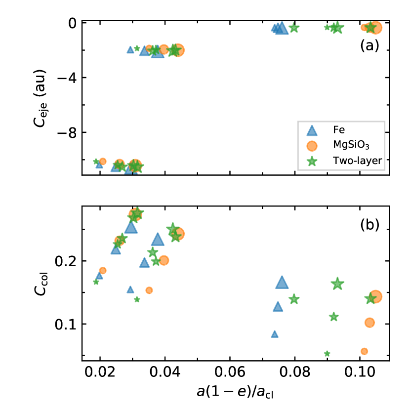
Figure 5: $C_{\rm eje}$ (a) and $C_{\rm col}$ (b) as a function of $a(1-e)/a_{\rm cl}$ for the configurations listed in Tables 1 and 2. The symbol size represents the scale of the planet’s mass. $C_{\rm eje}<0$ means the clump will not be ejected from the system. $C_{\rm col}>0$ means that the clump would collide with NS due to the perturbation.

The angular momentum of the clump is $J_{\rm cl}=M_{\star}m_{\rm cl}\left({Ga_{\rm cl}(1-e_{\rm cl}^{2})}/{M_{b}}\right)^{1/2}$, where $M_{\rm b}=M_{\star}+m_{\rm cl}$ is the total mass of the NS and the clump. In our case, $M_{\star}$ is much larger than $m_{\rm cl}$, so we have $M_{\rm b}\approx M_{\star}$. Let us define $J_{\rm cl,c}=J_{\rm cl}/(1-e_{\rm cl}^{2})^{1/2}$, which is the angular momentum of a circular orbit with the same semi-major axis, $a_{\rm cl}$, then the dimensionless angular momentum of the clump is $j_{\rm cl}=J_{\rm cl}/J_{\rm cl,c}=\sqrt{1-e_{\rm cl}^{2}}$. Due to the influence of the surviving planet, the clump’s specific angular momentum evolves on a timescale of $t_{\rm evo}=\left(\frac{1}{j_{\rm cl}}\frac{dj_{\rm cl}}{dt}\right)^{-1}$ (e.g. Antonini et al., 2014; Bode & Wegg, 2014; Hamers et al., 2022). In our framework, the timescale can be further expressed as

$$t_{\rm evo}=\left(\frac{1}{j_{\rm cl}}\frac{dj_{\rm cl}}{dt}\right)^{-1}\approx P_{\rm orb}^{\rm cl}\frac{1}{5\pi}\frac{M_{\star}}{m_{\rm pl}}\left[\frac{a(1-e)}{a_{\rm cl}}\right]^{3}\sqrt{1-e_{\rm cl}}.$$ (12)

It gives the time for the clump to evolve to $j_{\rm cl}\sim 0$, i.e. falling toward the NS.

Table 1: Typical parameters of the Fe/MgSiO₃ planet and the clumps stripped off from the planet.

Planet								Clump
$\rho_{\rm c}$	$m_{\rm pl}$	$R_{\rm pl}$	$\rho_{\rm c}/\bar{\rho}$	$P_{\rm orb}$	$a$	$e$		$a_{\rm cl}$	$P_{\rm orb}^{\rm cl}$	$e_{\rm cl}$	$t_{\rm evo}$
$(\rm g\,cm^{-3})$	($M_{\oplus}$)	($R_{\oplus}$)		(days)	(au)			(au)	(days)		(days)
Fe planet
25.65	4.57	1.15	1.54	10	0.10	0.943		0.08	6.73	0.927	4.74
				100	0.47	0.988		0.20	26.83	0.971	0.75
				1000	2.19	0.997		0.29	48.52	0.980	0.34
35.72	10.12	1.38	1.70	10	0.10	0.948		0.07	5.86	0.926	1.96
				100	0.47	0.989		0.16	19.41	0.967	0.40
				1000	2.19	0.998		0.21	30.68	0.975	0.22
48.32	18.12	1.56	1.85	10	0.10	0.951		0.07	5.14	0.925	1.01
				100	0.47	0.989		0.13	14.68	0.963	0.25
				1000	2.19	0.998		0.17	21.25	0.971	0.15
MgSiO3 planet
6.53	4.41	1.69	1.30	10	0.10	0.916		0.08	7.60	0.899	16.93
				100	0.47	0.982		0.24	37.30	0.965	2.03
				1000	2.19	0.996		0.41	81.58	0.979	0.72
7.95	9.95	2.12	1.38	10	0.10	0.919		0.08	6.94	0.898	7.23
				100	0.47	0.983		0.21	29.07	0.961	1.07
				1000	2.19	0.996		0.32	54.74	0.974	0.46
9.36	18.15	2.49	1.44	10	0.10	0.922		0.08	6.37	0.897	3.86
				100	0.47	0.983		0.18	23.43	0.957	0.68
				1000	2.19	0.996		0.26	39.86	0.970	0.33

Note: The mass, radius, and density of the planets are taken from the data in Fig. 2. Other parameters of the planets and clumps are calculated according to the equations given in the main text.

We have calculated the clump’s orbital period ($P_{\rm orb}^{\rm cl}$) and the corresponding evolution timescale of its angular momentum ($t_{\rm evo}$). They are plotted versus the planet mass in Fig. 6, and some typical parameters are also listed in Table 1. Our calculations are conducted for planets with three different orbital periods, i.e. $P_{\rm orb}=10$ days, $100$ days, and $1000$ days. From panel (a) of Fig. 6, we can see that for an Fe planet with a mass of $4.57M_{\oplus}$, the orbital period of the clump is $6.73$ days and the evolution timescale of its angular momentum is $4.74$ days for $P_{\rm orb}=10$ days. For $P_{\rm orb}=1000$ days, the orbital period of the clump is $48.52$ days and the evolutionary timescale of its angular momentum is $0.34$ days. For a Fe planet with $P_{\rm orb}=100$ days, the orbital period of the clump is $26.83$ days and the evolutionary timescale of its angular momentum is $0.75$ days for $m_{\rm pl}=4.57M_{\oplus}$. For $m_{\rm pl}=18.12M_{\oplus}$, the orbital period of the clump is $14.68$ days and the evolutionary timescale of its angular momentum is $0.25$ days. In general, for a planet with a particular mass, with the increase of the planet’s orbital period, the period of the clump also increases while the evolution timescale of its angular momentum decreases. On the other hand, for a planet with a particular orbital period, with the increase of the planet’s mass, both the clump’s orbital period and evolution timescale of angular momentum decrease. Panel (b) of Fig. 6 shows the cases for MgSiO₃ planets, which are largely similar to that of Fe planets.

Table 2: Typical parameters of two-layer planets (with Fe core and MgSiO₃ mantle) and the clumps stripped off from the planet.

Planet									Clump
$\rho_{\rm c}$	$m_{\rm pl}$	$R_{\rm pl}$	$\rho_{\rm c}/\bar{\rho}$	$f_{\rm Fe}$	$P_{\rm orb}$	$a$	$e$		$a_{\rm cl}$	$P_{\rm orb}^{\rm cl}$	$e_{\rm cl}$	$t_{\rm evo}$
$(\rm g\,cm^{-3})$	($M_{\oplus}$)	($R_{\oplus}$)		(%)	(days)	(au)			(au)	(days)		(days)
21.03	3.26	1.35	2.89	47	10	0.10	0.925		0.08	7.56	0.911	14.98
					100	0.47	0.984		0.24	36.71	0.969	1.82
					1000	2.19	0.997		0.40	79.43	0.981	0.65
31.10	9.83	1.83	3.50	47	10	0.10	0.930		0.08	6.61	0.909	4.69
					100	0.47	0.985		0.19	25.70	0.963	0.77
					1000	2.19	0.997		0.28	45.54	0.975	0.36
39.92	12.84	1.59	2.25	90	10	0.10	0.945		0.07	5.80	0.921	1.91
					100	0.47	0.988		0.16	18.97	0.964	0.39
					1000	2.19	0.997		0.21	29.73	0.973	0.22
27.33	17.10	2.41	4.05	6	10	0.10	0.923		0.08	6.38	0.898	3.90
					100	0.47	0.984		0.18	23.58	0.957	0.68
					1000	2.19	0.996		0.26	40.22	0.970	0.33
44.96	20.68	2.17	4.01	51	10	0.10	0.935		0.07	5.78	0.908	2.03
					100	0.47	0.986		0.15	18.81	0.958	0.42
					1000	2.19	0.997		0.21	29.40	0.969	0.23

Note: The mass, radius, and density of the two-layer planets are taken from the data in Fig. 1. Other parameters of the planets and clumps are calculated according to the equations given in the main text.

Table 2 presents some typical parameters for two-layer (Fe core and MgSiO₃ mantle) planets with different Fe-core fraction, $f_{\rm Fe}$. We see that with the increase in the planet’s orbital period, the period of the clump also increases, while the evolution timescale of its angular momentum decreases, which is similar to that of pure Fe planets and pure MgSiO₃ planets. However, for a fixed orbital period, when the mass of the planet increases, the changes of both the clump’s period and the evolution timescale of its angular momentum are quite different from that of pure Fe planets and pure MgSiO₃ planets. For example, in the case of $P_{\rm orb}=10$ days, the clump’s orbital period is $5.8$ days and the evolution timescale of its angular momentum is $1.91$ days for a planet mass of $12.84M_{\oplus}$ ($f_{\rm Fe}=90\%$). But for a planet mass of $17.10M_{\oplus}$ ($f_{\rm Fe}=6\%$), the clump’s orbital period is $6.38$ days and the evolution timescale of its angular momentum is $3.9$ days. It indicates that the tidal disruption process is affected by the composition of the planets.

We now estimate the clump’s travel time from the planet to the central NS. In our framework, partial disruption mainly occurs at the periastron. The time for a clump to return to the periastron ($t_{\rm ret}$) should equal to its orbital period (Zanazzi & Ogilvie, 2020; Mageshwaran & Mangalam, 2021; Rossi et al., 2021), i.e. $t_{\rm ret}\sim P_{\rm orb}^{\rm cl}$. After that, the clump’s angular momentum evolves on a timescale of $t_{\rm evo}$ under the influence of the gravitational perturbation from the remnant planet. Therefore, the time for the clump to travel to the NS can be approximated as $t_{\rm trav}\sim 2t_{\rm ret}+t_{\rm evo}$. For the configurations with $t_{\rm evo}\lesssim P_{\rm orb}^{\rm cl}$, we have $2P_{\rm orb}^{\rm cl}<t_{\rm trav}\lesssim 3P_{\rm orb}^{\rm cl}$, which means that the clumps will fall onto the NS within $\sim$ 2 — 3 orbital periods after their birth.

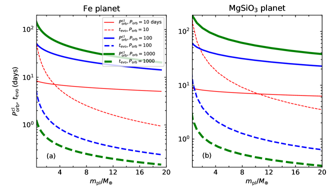
Figure 6: The orbital period of clumps (solid lines) and the evolution timescale of their angular momentum (dashed lines) plotted versus the planet’s mass. Panel (a) is for Fe planets and Panel (b) is for MgSiO₃ planets. The red, blue, and green lines correspond to the planets with orbital period of 10 days, 100 days, and 1000 days, respectively.

6 Discussions

In a binary system, the orbit will evolve due to various effects such as mass loss, gravitational wave (GW) radiation, tidal dissipation, and magnetic interactions. In this section, we discuss the effects of these evolutionary channels on our planetary systems.

1. Mass loss

   In our framework, the planet passes through the periastron repeatedly, and thus may experience multiple disruptions. Mass loss is a significant feature in the process, the effect of which on the orbit of the planet needs to be addressed. Especially, it should be clarified whether the planet still remains bound to the NS after multiple disruptions. During a partial disruption, the total mass loss is $\Delta m=\Delta m_{\rm 1}+\Delta m_{\rm 2}$, where $\Delta m_{\rm 1}$ and $\Delta m_{\rm 2}$ are the mass loss from the Lagrangian points $L_{1}$ and $L_{2}$, respectively. Usually, the mass loss is asymmetric with $\Delta m_{\rm 1}>\Delta m_{\rm 2}$. The surviving core thus could obtain a kick velocity due to the asymmetry, which is mainly determined by the mass difference defined as $\Delta m_{\rm 12}=\Delta m_{\rm 1}-\Delta m_{\rm 2}$. If the kick velocity is too large, then the surviving core could be scattered away from the NS. Similar processes have been extensively studied by many authors, but mainly on the tidal disruption of gaseous giant planets (Guillochon et al., 2011; Liu et al., 2013) and main sequence stars (Manukian et al., 2013; Gafton et al., 2015; Zhong et al., 2022). It is found that the mass difference ($\Delta m_{\rm 12}$) is very sensitive to $r_{\rm p}$. It generally decreases with the increase of $r_{\rm p}$. In our case, we have $r_{\rm p}\gtrsim 2r_{\rm td}$ ($\beta\lesssim 0.5$), then the mass difference of $\Delta m_{\rm 12}$ is essentially very small even for gaseous planets (Liu et al., 2013). Additionally, the planet is a rocky one, which further markedly reduces the mass difference. The impulse kick caused by such a $\Delta m_{\rm 12}$ is small and will not affect the orbit of the surviving core. As a result, it remains to be bound to the NS and continues to revolve around the host.

2. GWs and Tides

   The planet’s orbit may be affected by gravitational wave radiation and tidal dissipation. Here we consider these two factors. For the GW emission, we have calculated the decay time of the orbit ($t_{\rm gw}$) by using equation (6) of Vick et al. (2017). It is found that the decay time is very long, $t_{\rm gw}>10^{15}$ yr. For tidal dissipation, the decay time is even longer than the gravitational timescale (Vick et al., 2017). So, in our cases, the effects of both tidal dissipation and GW radiation can be neglected.

3. Alfvén-wave Drag

   It should be noted that an object moving around an NS could interact with the magnetosphere of the NS when the orbit radius is too small, producing some Alfvén wing structures. Such interactions will help the NS capture the object (Cordes & Shannon, 2008; Mottez & Heyvaerts, 2011). However, in our cases, the periastron is still relatively further away from the NS. As a result, for the clumps that are of the size of a few kilometers, the orbit decay time is very long (e.g. Zhang et al., 2021). Therefore, the Alfvén-wave drag is not a dominant mechanism for the orbit decay of the planet and clumps.

In short, the effects of mass loss, GWs, tides, and magnetic fields on the evolution of the planet and clumps are negligible in our framework.

7 Conclusions

In this study, we concentrate on the systems in which a rocky planet revolves around an NS in a highly elliptic orbit. The periastron of the planet is close to the NS, $r_{\rm p}\sim 2r_{\rm td}$, so that it will be partially disrupted every time it passes through the periastron, forming a multi-body system. The dynamical evolution of the clumps stripped off from the planet is investigated, taking into account the joint gravitational interactions of the NS and the surviving portion of the planet. The interactions among clumps are neglected for simplicity. As a result, the NS, the remnant planet, and a particular clump form a triple system. For the evolution of the clump in such a system, our conclusions are as follows:

• Gravitational perturbation from the remnant planet is a dominant factor that governs the evolution of the clump’s orbit. Due to the perturbation, the eccentricity of the clump orbit increases quickly so that its specific angular momentum decreases to almost zero on a timescale of several orbital periods, causing the clump to effectively collide with the NS.

• The detailed evolution of the clumps is significantly affected by the orbital parameters and the structure of the planet. We have examined three types of planets: pure Fe, pure MgSiO₃, and two-layer planets (Fe core and MgSiO₃ mantle). By assuming three typical orbital periods for the planet, i.e. 10 days, 100 days, and 1000 days, it is found that the evolutionary timescale of the clump’s angular momentum decreases with the increase of the orbital period and the planet’s mass. For planets with different compositions, the trend of change is similar for the evolution time timescale, but the exact values differ significantly.

Generally, we see that the clumps will collide with the NS shortly after their birth in a partial disruption event. The collision may lead to some kinds of electromagnetic transient events. In fact, it has been argued that the accretion of a small body by an NS can produce some special kinds of gamma-ray bursts (Colgate & Petschek, 1981). GRB 101225A may occur in this way (Campana et al., 2011). The collision of an asteroid with an NS may also account for X-ray bursts (Huang & Geng, 2014; Geng & Huang, 2015; Dai, 2020; Geng et al., 2020) and/or fast radio bursts (Geng & Huang, 2015; Dai et al., 2016; Smallwood et al., 2019; Dai, 2020; Geng et al., 2020; Dai & Zhong, 2020). However, the exact phenomenon associated with the collision will depend on many detailed factors, such as the composition and size of the clump, the magnetic field and spin period of the NS, the impact parameter, etc. It may even depend on the internal composition of the so-called neutron star, which may actually be a strange quark star (Geng et al., 2021; Nurmamat et al., 2022). A detailed case study on the various possible transients associated with the collision is still being conducted. Additionally, it should be noted that the partial tidal disruption of a rocky planet near the periastron is a very complicated process. In this study, we have taking some simplified assumptions on the size and shape of the clumps. To clarify these issues, numerical simulations on the tidal disruption process should be necessary, which is beyond the scope of this study.

8 Acknowledgments

We would like to thank the anonymous referee for helpful suggestions that led to significant improvement of our study This work is supported by the Chinese Academy of Sciences (CAS) “Light of West China” Program (No. 2019-XBQNXZ-B-016), the Natural Science Foundation of Xinjiang Uygur Autonomous Region (No. 2022D01A363), the Major Science and Technology Program of Xinjiang Uygur Autonomous Region (Nos. 2022A03013-1, 2022A03013-3), the National Natural Science Foundation of China (Grant Nos. 12041304, 12033001, 12273028, 12233002, 12041306, 12147103), the Youth Innovations and Talents Project of Shandong Provincial Colleges and Universities (Grant No. 201909118), National Key R&D Program of China (2021YFA0718500), National SKA Program of China No. 2020SKA0120300, the special research assistance project of the CAS, and by the Operation, Maintenance and Upgrading Fund for Astronomical Telescopes and Facility Instruments, budgeted from the Ministry of Finance of China (MOF) and administrated by the CAS.

Data Availability

The data underlying this article are available from the corresponding author upon reasonable request.

References

- Antonini & Perets (2012) Antonini F., Perets H. B., 2012, ApJ, 757, 27
- Antonini et al. (2014) Antonini F., Murray N., Mikkola S., 2014, ApJ, 781, 45
- Antonini et al. (2016) Antonini F., Chatterjee S., Rodriguez C. L., Morscher M., Pattabiraman B., Kalogera V., Rasio F. A., 2016, ApJ, 816, 65
- Bareither et al. (2008) Bareither C. A., Edil T. B., Benson C. H., Mickelson D. M., 2008, Journal of Geotechnical and Geoenvironmental Engineering, 134, 1476
- Benz & Asphaug (1999) Benz W., Asphaug E., 1999, Icarus, 142, 5
- Bhaskar et al. (2021) Bhaskar H., Li G., Hadden S., Payne M. J., Holman M. J., 2021, AJ, 161, 48
- Birch (1947) Birch F., 1947, Physical Review, 71, 809
- Bode & Wegg (2014) Bode J. N., Wegg C., 2014, MNRAS, 438, 573
- Brouwers et al. (2022) Brouwers M. G., Bonsor A., Malamud U., 2022, MNRAS, 509, 2404
- Brouwers et al. (2023) Brouwers M. G., Bonsor A., Malamud U., 2023, MNRAS, 519, 2646
- Campana et al. (2011) Campana S., et al., 2011, Nature, 480, 69
- Carrera et al. (2019) Carrera D., Raymond S. N., Davies M. B., 2019, A&A, 629, L7
- Colgate & Petschek (1981) Colgate S. A., Petschek A. G., 1981, ApJ, 248, 771
- Cordes & Shannon (2008) Cordes J. M., Shannon R. M., 2008, ApJ, 682, 1152
- Dai (2020) Dai Z. G., 2020, ApJ, 897, L40
- Dai & Zhong (2020) Dai Z. G., Zhong S. Q., 2020, ApJ, 895, L1
- Dai et al. (2016) Dai Z. G., Wang J. S., Wu X. F., Huang Y. F., 2016, ApJ, 829, 27
- Eggleton & Kiseleva (1995) Eggleton P., Kiseleva L., 1995, ApJ, 455, 640
- Faber et al. (2005) Faber J. A., Rasio F. A., Willems B., 2005, Icarus, 175, 248
- Gafton et al. (2015) Gafton E., Tejeda E., Guillochon J., Korobkin O., Rosswog S., 2015, MNRAS, 449, 771
- Geng & Huang (2015) Geng J. J., Huang Y. F., 2015, ApJ, 809, 24
- Geng et al. (2015) Geng J. J., Huang Y. F., Lu T., 2015, ApJ, 804, 21
- Geng et al. (2020) Geng J.-J., Li B., Li L.-B., Xiong S.-L., Kuiper R., Huang Y.-F., 2020, ApJ, 898, L55
- Geng et al. (2021) Geng J., Li B., Huang Y., 2021, The Innovation, 2, 100152
- Gezari (2021) Gezari S., 2021, ARA&A, 59, 21
- Goulinski & Ribak (2018) Goulinski N., Ribak E. N., 2018, MNRAS, 473, 1589
- Granvik et al. (2016) Granvik M., et al., 2016, Nature, 530, 303
- Grishin et al. (2018) Grishin E., Perets H. B., Fragione G., 2018, MNRAS, 481, 4907
- Guillochon & Ramirez-Ruiz (2013) Guillochon J., Ramirez-Ruiz E., 2013, ApJ, 767, 25
- Guillochon et al. (2011) Guillochon J., Ramirez-Ruiz E., Lin D., 2011, ApJ, 732, 74
- Gundlach & Blum (2016) Gundlach B., Blum J., 2016, A&A, 589, A111
- Hamers (2018) Hamers A. S., 2018, MNRAS, 478, 620
- Hamers et al. (2022) Hamers A. S., Perets H. B., Thompson T. A., Neunteufel P., 2022, ApJ, 925, 178
- He & Petrovich (2018) He M. Y., Petrovich C., 2018, MNRAS, 474, 20
- Hills (1975) Hills J. G., 1975, Nature, 254, 295
- Holsapple & Michel (2008) Holsapple K. A., Michel P., 2008, Icarus, 193, 283
- Hong et al. (2018) Hong Y.-C., Raymond S. N., Nicholson P. D., Lunine J. I., 2018, ApJ, 852, 85
- Howe et al. (2014) Howe A. R., Burrows A., Verne W., 2014, ApJ, 787, 173
- Huang & Geng (2014) Huang Y. F., Geng J. J., 2014, ApJ, 782, L20
- Huang & Yu (2017) Huang Y. F., Yu Y. B., 2017, ApJ, 848, 115
- Katz & Dong (2012) Katz B., Dong S., 2012, arXiv e-prints, p. arXiv:1211.4584
- Katz et al. (2011) Katz B., Dong S., Malhotra R., 2011, Phys. Rev. Lett., 107, 181101
- Kozai (1962) Kozai Y., 1962, AJ, 67, 591
- Kremer et al. (2019) Kremer K., D’Orazio D. J., Samsing J., Chatterjee S., Rasio F. A., 2019, ApJ, 885, 2
- Kuerban et al. (2019) Kuerban A., Geng J.-J., Huang Y.-F., 2019, in Xiamen-CUSTIPEN Workshop on the Equation of State of Dense Neutron-Rich Matter in the Era of Gravitational Wave Astronomy. p. 020027, doi:10.1063/1.5117817
- Kuerban et al. (2020) Kuerban A., Geng J.-J., Huang Y.-F., Zong H.-S., Gong H., 2020, ApJ, 890, 41
- Kurban et al. (2022) Kurban A., et al., 2022, ApJ, 928, 94
- Law-Smith et al. (2020) Law-Smith J. A. P., Coulter D. A., Guillochon J., Mockler B., Ramirez-Ruiz E., 2020, ApJ, 905, 141
- Li & Adams (2016) Li G., Adams F. C., 2016, ApJ, 823, L3
- Li et al. (2014a) Li G., Naoz S., Kocsis B., Loeb A., 2014a, ApJ, 785, 116
- Li et al. (2014b) Li G., Naoz S., Holman M., Loeb A., 2014b, ApJ, 791, 86
- Li et al. (2018) Li G., Hadden S., Payne M., Holman M. J., 2018, AJ, 156, 263
- Lidov (1962) Lidov M. L., 1962, Planetary and Space Science, 9, 719
- Lithwick & Naoz (2011) Lithwick Y., Naoz S., 2011, ApJ, 742, 94
- Liu et al. (2013) Liu S.-F., Guillochon J., Lin D. N. C., Ramirez-Ruiz E., 2013, ApJ, 762, 37
- Mageshwaran & Mangalam (2021) Mageshwaran T., Mangalam A., 2021, New Astron., 83, 101491
- Malamud & Perets (2020a) Malamud U., Perets H. B., 2020a, MNRAS, 492, 5561
- Malamud & Perets (2020b) Malamud U., Perets H. B., 2020b, MNRAS, 493, 698
- Manser et al. (2019) Manser C. J., et al., 2019, Science, 364, 66
- Manukian et al. (2013) Manukian H., Guillochon J., Ramirez-Ruiz E., O’Leary R. M., 2013, ApJ, 771, L28
- Mardling & Aarseth (2001) Mardling R. A., Aarseth S. J., 2001, MNRAS, 321, 398
- Mottez & Heyvaerts (2011) Mottez F., Heyvaerts J., 2011, A&A, 532, A22
- Naoz (2016) Naoz S., 2016, ARA&A, 54, 441
- Naoz et al. (2011) Naoz S., Farr W. M., Lithwick Y., Rasio F. A., Teyssandier J., 2011, Nature, 473, 187
- Naoz et al. (2013) Naoz S., Farr W. M., Lithwick Y., Rasio F. A., Teyssandier J., 2013, MNRAS, 431, 2155
- Naoz et al. (2017) Naoz S., Li G., Zanardi M., de Elía G. C., Di Sisto R. P., 2017, AJ, 154, 18
- Nurmamat et al. (2022) Nurmamat N., Huang Y.-F., Geng J.-J., Kurban A., Li B., 2022, arXiv e-prints, p. arXiv:2211.12026
- Otegi et al. (2020) Otegi J. F., Bouchy F., Helled R., 2020, A&A, 634, A43
- Perets & Kratter (2012) Perets H. B., Kratter K. M., 2012, ApJ, 760, 99
- Petrovich (2015) Petrovich C., 2015, ApJ, 808, 120
- Pohl & Britt (2020) Pohl L., Britt D. T., 2020, Meteoritics & Planetary Science, 55, 962
- Rossi et al. (2021) Rossi E. M., Stone N. C., Law-Smith J. A. P., Macleod M., Lodato G., Dai J. L., Mandel I., 2021, Space Sci. Rev., 217, 40
- Ryu et al. (2020) Ryu T., Krolik J., Piran T., Noble S. C., 2020, ApJ, 904, 100
- Seager et al. (2007) Seager S., Kuchner M., Hier-Majumder C. A., Militzer B., 2007, ApJ, 669, 1279
- Seto (2013) Seto N., 2013, Phys. Rev. Lett., 111, 061106
- Shevchenko (2017) Shevchenko I. I., 2017, The Lidov-Kozai Effect - Applications in Exoplanet Research and Dynamical Astronomy. Astrophysics and Space Science Library Vol. 441, Springer Cham, doi:10.1007/978-3-319-43522-0
- Smallwood et al. (2019) Smallwood J. L., Martin R. G., Zhang B., 2019, MNRAS, 485, 1367
- Smith et al. (2018) Smith R. F., et al., 2018, Nature Astronomy, 2, 452
- Sridhar & Tremaine (1992) Sridhar S., Tremaine S., 1992, Icarus, 95, 86
- Swift et al. (2012) Swift D. C., et al., 2012, ApJ, 744, 59
- Toonen et al. (2022) Toonen S., Boekholt T. C. N., Portegies Zwart S., 2022, A&A, 661, A61
- Vanderburg et al. (2015) Vanderburg A., et al., 2015, Nature, 526, 546
- Veras & Scheeres (2020) Veras D., Scheeres D. J., 2020, MNRAS, 492, 2437
- Veras et al. (2014) Veras D., Leinhardt Z. M., Bonsor A., Gänsicke B. T., 2014, MNRAS, 445, 2244
- Vick et al. (2017) Vick M., Lai D., Fuller J., 2017, MNRAS, 468, 2296
- Zanazzi & Ogilvie (2020) Zanazzi J. J., Ogilvie G. I., 2020, MNRAS, 499, 5562
- Zhang & Lin (2020) Zhang Y., Lin D. N. C., 2020, Nature Astronomy, 4, 852
- Zhang et al. (2021) Zhang Y., Liu S.-F., Lin D. N. C., 2021, ApJ, 915, 91
- Zhang et al. (2023) Zhang E., Naoz S., Will C. M., 2023, arXiv e-prints, p. arXiv:2301.08271
- Zhong et al. (2022) Zhong S., Li S., Berczik P., Spurzem R., 2022, ApJ, 933, 96