Abstract

The review analyzes the fundamental principles which Artificial Intelligence should be based on in order to imitate the realistic process of taking decisions by humans experiencing emotions. Two approaches are considered, one based on quantum theory and the other employing classical terms. Both these approaches have a number of similarities, being principally probabilistic. The analogies between quantum measurements under intrinsic noise and affective decision making are elucidated. It is shown that cognitive processes have many features that are formally similar to quantum measurements. This, however, in no way means that for the imitation of human decision making Affective Artificial Intelligence has necessarily to rely on the functioning of quantum systems. The analogies between human decision making and quantum measurements merely demonstrate formal common properties in their functioning. It is in this sense that one has to understand quantum operation of Artificial Intelligence. Appreciating the common features between quantum measurements and decision making helps for the formulation of an axiomatic approach employing only classical notions. Artificial Intelligence, following this approach, operates similarly to humans, by taking into account the utility of the considered alternatives as well as their emotional attractiveness. Affective Artificial Intelligence, whose operation takes account of the cognition-emotion duality, avoids numerous behavioural paradoxes of traditional decision making. A society of intelligent agents, interacting through the repeated multistep exchange of information, forms a network accomplishing dynamic decision making based on the evaluation of utility and affected by the emotional attractiveness of alternatives. The considered intelligent networks can characterize the operation of either a human society of affective decision makers, or the brain composed of neurons, or a typical probabilistic network of an artificial intelligence.

Keywords: artificial intelligence, quantum measurements, quantum intrinsic noise, affective decision making, cognition-emotion duality, behavioural paradoxes, dynamic decision making, collective decision making, probabilistic networks

Contents

1. Introduction

2. Measurements under intrinsic noise

2.1. Quantum algebra of events

2.2. Operationally testable events

2.3. Modes of intrinsic noise

2.4. Noise-decorated alternatives

2.5. Quantum probability space

2.6. Quantum-classical correspondence

2.7. Probability of superposition states

2.8. Alternative-noise entanglement

2.9. Entanglement production by measurements

2.10. Time dependence of probability

2.11. Quantum state reduction

2.12. Consecutive measurements of alternatives

2.13. Immediate consecutive measurements

2.14. Synchronous noiseless measurements

2.15. Synchronous measurements under noise

2.16. Swap order relations

2.17. Quantum versus classical probabilities

2.18. Quantum decision theory

3. Affective decision making

3.1. Evolutionary origin of emotions

3.2. Problems in decision making

3.3. Behavioural probabilities of alternatives

3.4. Quantification of utility factor

3.5. Magnitude of attraction factor

3.6. Multiple attraction factors

3.7. Problems in classifying attractiveness

3.8. Explicit attraction factors

3.9. Buridan’s donkey problem

3.10. Kahneman-Tversky lotteries

3.11. Verification of quarter law

3.12. Contextuality of attraction factors

3.13. Choice between bundled alternatives

3.14. Quantum versus classical consciousness

4. Resolution of behavioural paradoxes

4.1. St. Petersburg paradox

4.2. Martingale illusion

4.3. Allais paradox

4.4. Independence paradox

4.5. Ellsberg paradox

4.6. Prisoner dilemma

4.7. Disjunction effect

4.8. Conjunction fallacy

4.9. Disposition effect

4.10. Ariely paradox

4.11. Decoy effect

4.12. Planning paradox

4.13. Preference reversal

4.14. Preference intransitivity

4.15. Order effects

5. Networks of intelligent agents

5.1. Multistep decision making

5.2. Types of interactions and memory

5.3. Networks with uniform memory

5.4. Network with mixed memory

5.5. Dynamic regimes of preferences

5.6. Attenuation of emotion influence

5.7. Continuous decision making

5.8. Discrete versus continuous processes

5.9. Time discounting of utility

5.10. Collective network operation

6. Conclusion

1 Introduction

Artificial Intelligence is understood as intelligence demonstrated by machines, as opposed to natural intelligence displayed by animals including humans. The main Artificial Intelligence textbooks define the field as the study of artificial intelligent systems perceiving the information obtained from the environment and taking decisions and actions for the goal attainment [1, 2, 3, 4, 5, 6]. There is wide agreement among artificial intelligence researchers that to be called intelligence, it is required to be able to use logical strategy and make judgments under uncertainty.

A system possessing intelligence is termed an intelligent agent. That system, evaluating the available information, is able to take autonomous actions and decisions directed to the achievement of the desired goals and may improve its performance with learning or using obtained knowledge [1, 2, 3, 4, 5, 6]. Often, the term intelligent agent is applied to systems possessing artificial intelligence. However the intelligent agent paradigm is closely related and employed with respect to agents in economics, in cognitive science, ethics, philosophy, as well as in many interdisciplinary socio-cognitive modeling and simulations. Generally, from the technical or mathematical point of view, the notion of intelligent agent can be associated with either real or artificial intelligence. An intelligent agent could be anything that makes decisions, as a person, firm, machine, or software.

In this review, we concentrate on one of the most difficult and important problems of Artificial Intelligence, that is on the mechanism of taking decisions similarly to this process in humans, whose decisions practically always are accompanied by emotions. The achievement of human-level machine intelligence has been a principal goal from the beginning of works on Artificial Intelligence [1, 2, 3, 4, 5, 6]. The key-point of the present review is the description of how affective decision making could be mathematically formalized to the level sufficient for the functioning of Artificial Intelligence imitating human decision processes in which emotions are an inevitable part. Below, talking about Artificial Intelligence we keep in mind Affective Artificial Intelligence.

In order to formulate the basic operational algorithms of Affective Artificial Intelligence, it is necessary to develop a mathematical description of human affective decision making. The problem of emotion quantification consists of two sides. One side is the assessment of emotions experienced by a subject as reactions on external events, e.g., hearing voice or looking at pictures. The arising emotions can include happiness, anger, pleasure, disgust, fear, sadness, astonishment, pain, and so on. The severity or intensity of such emotions can be estimated by studying the expressive forms manifesting themselves in motor reactions, such as facial expressions, pantomime, and general motor activity, and by measuring physiological reactions, such as the activity of the sympathetic and parasympathetic parts of the autonomic nervous system, as well as the activity of the endocrine glands. Vegetative manifestations of emotions can be noticed by studying changes in the electrical resistance of the skin, the frequency and strength of heart contractions, blood pressure, skin temperature, hormonal and chemical composition of the blood, and like that. There exists a vast literature on the methods of emotion detection and appraisal in speech, facial expressions, and body gestures [7, 8]. The study and development of systems and devices that can recognize, interpret, process, and simulate human affects is named Affective Computing [9, 10]. These problems will not be touched in the review.

The other side of the story is the challenge of characterizing how emotions influence decision making. To formulate the principles of functioning of Affective Artificial Intelligence in the process of taking decisions, it is necessary to be able to quantify the role of emotions in this process. It is this objective that is in the center of the present review.

This goal confronts the basic problem of how emotions, arising in the process of decision making, could be defined and quantified. It seems to be too difficult, if possible at all, to develop a formalized quantification of emotions allowing for the selection, in the presence of emotions, of an optimal alternative in the cognitive process of making decisions. The mathematical description of emotion influence in the process of decision making is the hard problem that has not found yet a comprehensive solution [11].

Difficulties start with the fact that there is no a unique generally accepted definition of what is emotion as compared to cognition. It is possible to mention the long-standing dispute about whether emotion is primary and independent of cognition [12, 13], or secondary and always dependent upon cognition [14, 15], although there is the point of view that this dispute is largely semantic, being induced by dissimilar definitions [16].

The studies on brain organization often support the assumption that there is a considerable degree of functional specialization and that many regions of brain can be conceptualized as either affective or cognitive. Popular examples are the amygdala in the domain of emotion and the lateral prefrontal cortex in the case of cognition. However, there are arguments [17, 18] that complex cognitive-emotional behaviours have their basis in dynamic coalitions of networks of brain areas, none of which should be conceptualized as specifically affective or cognitive. Different brain areas exhibit a high degree of connectivity for regulating the flow and integration of information between brain regions, which results in the intense cognitive-emotional interactions. Usually, under “emotions” one understands just a placeholder for something much broader than emotions in a narrow sense, including affective processes in general [19]. There are arguments that the notions of emotion, cognition, and the related phenomena can be more precisely defined in a functional framework, for example in terms of behavioural principles [20], with respect to emotion taxonomy [21], to emotion regulation [22], or studying the emotion appraisal during the dynamics of the emotion process [23, 24, 7]. More references on the definition of emotions and their relation to cognition can be found in the surveys [25, 26, 27].

The functional framework keeps in mind the operational separation of cognition and emotion as the notions related to the process of decision making that comprises two sides, reasoning and affective [11, 28]. Under the reasoning side one means the ability of formulating explicit rules allowing for a normative choice. And the affective side implies the possibility of making a choice being influenced by emotions that not always allow for explicit formal prescriptions. The reasoning-affective dichotomy in decision making is often called rational-irrational duality [29]. As is explained above, there is no strictly speaking uniquely defined and absolutely separated notions of cognitive and affective, as well as of rational and irrational. However, our goal is not to plunge into semantic debates, but to describe an approach taking into account two aspects of decision making, normative allowing for the explicit evaluation of utility and affective that seems to avoid the characterization by prescribed formal rules. The kaleidoscope of emotions can be quite ramified and not allowing for sharp categorical definitions, because of which it is labeled [23, 24, 7] as idiosyncratic and fuzzy. This fuzziness is the main obstacle in the attempts of quantifying the influence of emotions on decision making.

Thus the principal difference between a standard programmed robot or computer and human-type intelligence is the cognition-emotion duality of human consciousness in the process of taking decisions. For clarity, one can talk about human intelligence, although the same duality in decision making is typical of practically all alive beings, as numerous empirical studies prove. The animals likely feel a full range of emotions, including fear, joy, happiness, shame, embarrassment, resentment, jealousy, rage, anger, love, pleasure, compassion, respect, relief, disgust, sadness, despair, and grief [30].

The cognition-emotion duality of human consciousness, exhibited when taking decisions, combines rational conscious evaluation of utility of the intended actions with irrational subconscious emotions. The latter are especially noticeable in decisions under risk and uncertainty. This duality is the cause of a number of behavioural paradoxes in classical decision making, when human actions contradict expected utility theory. So, in order to formulate explicit algorithms for the operation of Affective Artificial Intelligence, comprising cognition-emotion duality, it is necessary to develop an adequate theory of affective decision making that could give realistic predictions under uncertainty.

The existence of the cognition-emotion duality in decision making hints on the possibility of its description by resorting to the techniques of quantum theory, in which there also exists duality, the so-called particle-wave duality [31]. Although the nature of these notions in physics and decision theory is rather different, but, probably, the mathematical techniques of quantum theory could hint on the similar description of both phenomena. Bohr [32, 33] was the first to assume that the functioning of the human brain could be described by the techniques of quantum theory. Since then, there have appeared numerous publications discussing the possibility of directly applying quantum techniques for characterizing the process of human decision making. These discussions, assuming that consciousness is quantum or quantum-like have been summarized in many review works, e.g. [34, 35, 36, 37, 38, 39], where numerous references on different attempts of applying quantum techniques to the description of consciousness are cited.

It is necessary to accept that many researchers are rather sceptical with regard to the parallelism between quantum physics and cognitive processes because of the following reasons:

(i) First of all, according to the current neurophysiological knowledge, the brain is in no way a quantum system, hence, it has nothing to do with quantum consciousness. The assumption that the brain’s neurons act as miniature quantum devices, thus that the brain functions similarly to a quantum computer [40, 41] has been justly criticized [42] by showing that decoherence effects do not allow for neurons to act as quantum objects. This does not exclude that some quantum processes do exist in the brain, which are studied in quantum biophysics [43, 44]. Nevertheless, the brain as a whole and its functioning seem to have nothing to do with quantum theory.

(ii) The above objection is usually refuted by saying that the possibility of describing human thinking processes by means of quantum theory does not require the assumption that human brains are some quantum systems. Instead, it holds that, although the brain is not a quantum object, but cognition and the process of human thinking can be mathematically formalized into the language of quantum theory. This is similar to the situation presented by the theory of differential equations, which was initially developed for describing the motion of planets. But now the theory of differential equations is employed everywhere, being just an efficient mathematical tool not necessarily related to planet motion. In the same way, quantum theory may provide a convenient framework for the mathematical description of thinking processes. The critics, however, insist that the analogies are superficial, do not prescribe practical recipes, and sometimes even contradict empirical data qualitatively [45, 46].

(iii) Moreover, the simple logic teaches us that, if the brain is a classical object, then its functioning should be described by classical equations, since it is exactly its properties, including functioning, that classify an object as classical or quantum. If the properties of an object cannot in principle be described by a classical theory, but allow for only quantum description, then this object is quantum, which contradicts our current knowledge on the brain.

(iv) The direct use of quantum theory for describing decision making introduces a large number of unknown parameters and ambiguous notions that cannot be characterized on the level of observable quantities associated with decision making. For instance, what is a Hamiltonian in psychological processes? How to define and measure numerous coefficients entering wave functions describing the brain states? What is the evolution equation for statistical operators characterizing the brain? And a lot of other ambiguously defined notions appear [47].

(v) The most important goal of any theory is the ability of predicting quantitative results that could be verified in experiment. However, none of the purely quantum variants of decision making has ever predicted some numerical data. The maximum what can be done is the consideration of particular cases and fitting parameters for the assumed interpretation of these cases. In order to extract quantitative information from the derived quantum relations, it is necessary to complement them by a number of assumptions not related to quantum techniques. In that sense the complicated quantum substructure becomes excessive, similarly to the excessiveness of nonlocal hidden variables for explaining quantum phenomena [48].

(vi) The fact that some events in decision making can qualitatively be interpreted as due to quantum processes does not exclude the possibility of other interpretations in terms of classical language. According to the Occam’s razor principle, the simplest of competing theories has to be preferred to the more complex, so that explanations of unknown phenomena should be sought first in terms of known quantities. Hence quite complicated theories based on quantum formulas are to be disregarded in favor of much simpler explanations based on classical notions, provided these exist. Entities should not be multiplied beyond necessity. The simplest theory is the best [49].

To understand whether the functioning of consciousness is described by quantum or classical rules is important, since, depending on the involved formalism, the operation of artificial intelligence has to be characterized in the same language. Examining the above objections to the use of quantum techniques for the formalization of decision making, it is possible to say the following: First, although at the present time, the influence of quantum effects on the functioning of the brain has not been convincingly argued, it cannot be absolutely excluded. Second, even if actual quantum effects play no role in the brain operation and consciousness does not need quantum description, the investigation of the analogies between decision making and quantum processes can enrich both of them suggesting their more profound comprehension. The peculiarities of quantum phenomena, that are better conceived, can give hints on the ways of characterizing consciousness functioning.

The point of view advocated in this review can be summarized as follows: The brain is a classical object, hence its basic property, that is consciousness, by definition, has to be classical. Otherwise it would be a meaninglessness to say that a classical object has quantum properties. Nevertheless, there exists a number of formal analogies in the description of quantum measurements and decision making. These analogies need to be carefully investigated for two reasons:

(i) Although being formal, the analogies between different phenomena very often suggest concrete practical ways for describing these phenomena.

(ii) Borrowing some ideas from the nominal analogies between two different approaches helps to compare these approaches and to choose the more efficient and simple theory.

The formal analogy between quantum and conscious phenomena has been noticed long time ago by von Neumann, who mentioned that the quantum theory of measurements can be interpreted as decision theory [50]. This concept has been developed by other researchers, for instance by Benioff [51, 52]. Thus quantum measurement is analogous to decision making, hence the measurement of an observable is similar to the choice of an alternative in decision making. Accepting these analogies, we can go further. Keeping in mind that emotions appear subconsciously during the process of decision making, they can be associated with intrinsic noise produced by a measuring device during the measurement procedure. In that way, the observable-noise duality is equivalent to the cognition-emotion duality. In the same way as in physical measurements the detection of signals can be either hindered by noise or the addition of the appropriate amount of noise can boost a signal and hence facilitate its detection [53, 54], in decision processes, emotions can either hinder or facilitate decision making.

In quantum measurements, there can exist observable-noise entanglement, which in decision making corresponds to correlations mimicking cognition-emotion entanglement. If the intrinsic noise is presented as a superposition of several modes, then there appears noise interference, hence there can arise the emotion interference. In that way, it is possible to expect different similarities between quantum measurements and decision making. So, even if consciousness does not function exactly by the same rules as quantum measurements, but anyway the many found similarities can provide useful hints for formalizing the operation of decision procedures, hence for the creation of artificial intelligence.

Concluding, in order to avoid confusion, it is necessary to stress what the review is about and what are not the review aims. This is in no way a survey of the general field of quantum techniques applied to the characterization of consciousness, because of which thousands of articles on such applications are not discussed, but only the main books are cited, where the vast number of references can be found. Concentrating on the ideas and methods for emotion quantification, citations are given only to those works where the role of emotions in decision making is studied and especially where practical methods of their description are discussed, but we do not plunge into the ocean of papers where no these problems are touched upon. While in the majority of works discussing the applications of quantum theory to consciousness neither the role of emotions is considered, nor their quantification is touched at all.

The very first requirement in the way of creating human-like artificial intelligence is the formulation of explicit mathematical rules of its operation. This paper does not pretend to describe all technical stages of actual artificial intelligence functioning, but it aims at formulating explicit mathematical algorithms for the operation of a human-like artificial intelligence in the process of taking decisions. Without a mathematical description of such rules and algorithms, no device can be modeled. But in order to mathematically formulate the process of choice in human-like decision making to be implemented by an artificial intelligence, it is compulsory to understand and mathematically describe the process of choice by humans, whose actions an artificial intelligence is planned to mimic. Therefore the pivotal aim of the paper is to analyze the combination of the following problems, whose solution is necessary for the mathematical formulation of decision making by an intelligence, whether human-like artificial or human:

(1) The analysis of the role of emotions in decision making and survey of the related literature, whether it employs quantum or classical language. This is necessary for understanding the basic qualitative principles of Affective Intelligence Processing

(2) The exposition of a practical way for emotion quantification in the process of taking decisions. This is a prerequisite for the formation of an Affective Artificial Intelligence requiring, for its functioning, the existence of explicit quantitative algorithms.

(3) The comparison of two ways, quantum and classical, for the formulation of the practical principles of Affective Decision Making. This is compulsory for selecting the most appropriate method that would be self-consistent, simple, and providing quantitative recipes for its operation.

(4) The comprehension of how the classical approach has to be modified in order to provide the same practical results as with the use of quantum techniques. Again, this is impossible to understand without a comparison of both approaches, quantum and classical. Otherwise, the reader would constantly exclaim: Why this or that assumption has been made? Where this or that formula has appeared from?

These goals are realized in the review. An exhaustive survey of literature discussing the role of emotions in decision making is given. The attempts of emotion quantification are described being based on the available literature. As is evident from numerous given citations, there are plenty of papers discussing the role of emotions in classical terms. The detailed comparison of quantum and classical techniques is given. It is shown that the classical approach can be modified by taking account of emotions, in such a way that to give the same results as in the language of quantum decision theory. For example, all paradoxes of classical decision making can be quantitatively explained without any use of quantum theory.

However, without comparing the two different approaches for taking into account emotions, it would be impossible: First, to make a conclusion which of them is preferable, and second, how it would be necessary to modify the classical theory so that it would give the same results as the quantum approach. Therefore all parts of the review are of equal importance and would lose sense being separated. Thus it is impossible to justify one of the approaches without comparing it with the other. On the other side, after different approaches are formulated, they can be employed independently and their effectiveness compared.

The layout of the review is as follows. In Sec. $2$, the general theory of quantum measurements in the presence of intrinsic noise is introduced. The analogies with decision making are emphasized. Assuming that the functioning of noisy quantum measurements is similar to that of affective decision making suggests the general framework for the latter. The comparison of a quantum and a modified classical approaches does not merely provide interesting analogies, but it allows for the formulation of the most simple and effective theory of Affective Decision Making.

Quantum techniques, of course, are not a common knowledge and can strongly hinder the use of quantum theory for practical applications. Therefore, if the same phenomena can be described in quantum language and also in classical terms, it is reasonable to resort to the simpler classical approach, but not to play science specially complicating the consideration with fashionable terminology. The theory has to be as simple as possible, in order that it could be straightforwardly employed by anyone, including those who may not know quantum techniques. This concerns decision theory as well, which can be developed as a branch of quantum theory or can be reformulated into an axiomatic form that, from one side mimics some quantum operations and structures, but, from the other side, does not require the knowledge of quantum terminology. Section 3 accomplishes this goal showing that the theory of affective decision making can be formulated in an axiomatic way that does not need to resort to quantum theory. Being formulated in mathematical terms, affective decision theory can be implemented for the operation of artificial intelligence. Section 4 considers the famous behavioural paradoxes in decision making and shows that, on the aggregate level, these paradoxes do not arise in the frame of the affective decision theory. In that sense, an artificial intelligence, obeying the rules of this theory, will act as a typical human decision maker. In Section 5, the structure of networks composed of intelligent agents taking decisions in the presence of emotions is described. Section 6 concludes.

2 Measurements under intrinsic noise

One of the main points advocated in the present review is the existence of an analogy between human emotions in decision making and intrinsic noise in quantum measurements. This obliges us to investigate the structure of quantum probability for measurements under intrinsic noise in order to find out the answers to two principal questions:

1. Can this analogy be employed for developing affective decision theory that could be sufficiently formalized for being useful for describing the operation of human-level artificial intelligence?

2. Whether this analogy is merely nominal or it goes deeper than that, requiring the use of quantum techniques for adequately representing behavioural decision making?

In physics, noise is modeled by introducing concrete noise terms into Hamiltonians or evolution equations and prescribing the corresponding distributions [53, 54, 55, 56]. Our aim here is not the analysis of concrete models, but the study of the general structure of probabilities for quantum events, decorated by the presence of intrinsic noise [57]. This is because we wish to compare these probabilities with those arising in decision theory. However the explicit nature of intrinsic noise, mimicking emotions, appearing in the process of taking decisions, is not known. Thus only general structures can be compared. In parallel with the physics terminology, we shall mention decision-making analogies of the considered notions. The mentioned analogies do not imply that the process of taking decisions by humans has to be necessarily treated as a quantum procedure, but conversely, this rather means that quantum measurements can be handled as formally similar to decision making [51, 52, 58, 59, 60]. The most important analogy is between intrinsic noise in quantum measurements and emotions in decision making [60, 61].

2.1 Quantum algebra of events

Let us consider quantum events $A_{n}$, enumerated with the index $n=1,2,\ldots$. For concreteness, we consider a discrete index $n$, while in general it could be continuous. Events can be the results of measurements for observable quantities. In decision theory, an event can be the choice of a particular alternative from the given set of alternatives. The collection of quantum events forms a ring [62, 63],

$$\mathbb{A}=\{A_{n}:~{}n=1,2,\ldots\}$$ (2.1)

possessing two binary operations, addition and conjunction. Addition, or union, or disjunction, implies that for any $A,B\in\mathbb{A}$ there is the union $A\cup B\in\mathbb{A}$, meaning either $A$ or $B$ and enjoying the properties

$$A\bigcup B=B\bigcup A\qquad({\rm commutativity})\;,$$

$$A\;\bigcup\;\left(B\;\bigcup\;C\right)=\left(A\;\bigcup\;B\right)\;\bigcup\;C\qquad({\rm associativity})\;,$$

$$A\;\bigcup\;A=A\qquad({\rm idempotency})\;.$$

Conjunction, or multiplication, means that for any $A,B\in\mathbb{A}$ there exists $A\cap B\in\mathbb{A}$ implying both $A$ and $B$ and having the properties

$$A\;\bigcap\;\left(B\;\bigcap\;C\right)=\left(A\;\bigcap\;B\right)\;\bigcap C\;\qquad({\rm associativity})\;,$$

$$A\;\bigcap\;A=A\qquad({\rm idempotency})\;.$$

In general, conjunction is not commutative,

$$A\;\bigcap\;B\neq B\;\bigcap\;A\qquad({\rm no\;commutativity})\;,$$

and not distributive,

$$A\;\bigcap\;\left(B\;\bigcup\;C\right)\neq\left(A\;\bigcap\;B\right)\;\bigcup\;\left(A\;\bigcap\;C\right)\qquad({\rm no\;distributivity})\;.$$

The ring $\mathbb{A}$ includes the identical event $1\in\mathbb{A}$, which is an event that is identically true. For this event,

$$A\;\bigcap\;1=1\;\bigcap\;A=A\;,\qquad A\;\bigcup\;1=1\;,\qquad 1\;\bigcup\;1=1\;.$$

Also, there exists an impossible event $0\in\mathbb{A}$, which is identically false, so that

$$A\;\bigcap\;0=0\;\bigcap\;A=0\;,\qquad A\;\bigcup\;0=A\;,\qquad 0\;\bigcup\;1=1\;.$$

The events for which $A\cap B=B\cap A=0$ are called disjoint or orthogonal. Note that one often simplifies the above notation by denoting the addition as $A\cup B\equiv A+B$ and the conjunction as $A\cap B\equiv AB$.

For each event $A\in\mathbb{A}$, there exists a complementary, or negating, event $\overline{A}\in\mathbb{A}$, for which

$$A\;\bigcup\;\overline{A}=1\;,\qquad A\;\bigcap\;\overline{A}=\overline{A}\;\bigcap\;A=0\;,\qquad\overline{0}=1\;,\qquad\overline{1}=0\;.$$

The absence of distributivity can be demonstrated by the simple example [62]. Consider two events $B_{1}$ and $B_{2}$ whose union forms unity, $B_{1}\cup B_{2}=1$. And assume that both $B_{1}$ and $B_{2}$ are orthogonal to a non-trivial event $A\neq 0$, so that $A\cap B_{1}=A\cap B_{2}=0$. By this definition, $A\cap(B_{1}\cup B_{2})=A\cap 1=A$. If the property of distributivity were true, then it would be $(A\cap B_{1})\cup(A\cap B_{2})=0$. Since, by assumption, $A\neq 0$, the property of distributivity does not hold.

The concept of non-distributivity in quantum physics can be illustrated by the example of spin measurements [63]. Let the spin projection of a particle with spin 1/2 be measured. Suppose $B_{1}$ is the event of measuring the spin in the up state with respect to the $z-$axis, whereas $B_{2}$ is the event of measuring the spin in the down state along this axis. The spin can be either up or down, hence $B_{1}\cup B_{2}=1$. Assume that $A$ is the event of measuring the spin along an axis in the plane orthogonal to the $z-$axis, say along the $x-$axis. Since the spin cannot be measured simultaneously along two orthogonal axes, it is found either measured along one axis or along another axis, but cannot have components on both axes simultaneously. Hence, $A\cap B_{1}=A\cap B_{2}=0$. At the same time, $A\cap(B_{1}\cup B_{2})=A\neq 0$. Therefore, there is no distributivity of events in the spin measurement.

2.2 Operationally testable events

An event is termed operationally testable, when it can be quantified by means of measurements. In physics, one measures observable quantities. For example, in quantum physics, one can measure the eigenvalues of a Hermitian operator corresponding to an observable. In decision making, one makes decisions by choosing preferable alternatives from the given set. Quantum measurements can be treated as a kind of decision making [50, 51, 52, 58, 64, 65].

Let us consider a set of alternatives (2.1) representing, e.g., a set of eigenvalues of an operator in quantum physics or a set of alternatives in decision theory. In quantum theory, each $A_{n}$ can be put into correspondence to a vector (state of an alternative) $|A_{n}\rangle$ in a Hilbert space $\mathcal{H}_{A}$. For simplicity, we keep in mind nondegenerate spectra of Hermitian operators. The vectors $|A_{n}\rangle$ can be orthonormalized,

$$\langle\;A_{m}\;|\;A_{n}\;\rangle=\delta_{mn}\;.$$ (2.2)

Here and in what follows, the Dirac bracket notation [66] is employed. The Hilbert space $\mathcal{H}_{A}$ can be defined as the closed linear envelope

$${\cal H}_{A}={\rm span}\;\{|\;A_{n}\;\rangle\}\;.$$ (2.3)

In quantum decision theory, this is called the space of alternatives.

Each alternative $A_{n}$ is represented by a projection operator

$$\hat{P}(A_{n})=|\;A_{n}\;\rangle\langle\;A_{n}\;|$$ (2.4)

enjoying the property

$$\hat{P}(A_{m})\;\hat{P}(A_{n})=\delta_{mn}\;\hat{P}(A_{n})\;.$$

The latter means that the projection operators are idempotent and the alternatives of the ring $\mathbb{A}$ are mutually incompatible. The projection operators satisfy the resolution of unity

$$\sum_{n}\hat{P}(A_{n})=\hat{1}_{A}\;,$$ (2.5)

where $\hat{1}_{A}$ is the identity operator in ${\cal H}_{A}$. The complete family of the projection operators forms the projection-valued operator measure on ${\cal H}_{A}$ with respect to set (2.1).

In quantum physics there can happen degenerate spectra, when for an $A_{n}$ there correspond several vectors $|A_{n_{i}}\rangle$, with $i=1,2,\ldots$. Then the projection operator associated with $A_{n}$ is

$$\hat{P}(A_{n})=\sum_{i}\hat{P}(A_{n_{i}})\;,\qquad\hat{P}(A_{n_{i}})\equiv|\;A_{n_{i}}\;\rangle\langle\;A_{n_{i}}\;|\;.$$

If one wishes to avoid the problem of degeneracy, one slightly modifies the considered system by introducing infinitesimal terms lifting the degeneracy connected with some kind of symmetry, as has been mentioned by von Neumann [50] and elaborated by Bogolubov [67, 68, 69]. Similarly, in decision theory, the problem of degeneracy can be easily avoided by reclassifying the alternatives under consideration [70, 71]. Thus for decision theory, it is sufficient to consider the situation with no degeneracy.

2.3 Modes of intrinsic noise

Any measurement is accompanied by some kind of noise that can be of two types, extrinsic and intrinsic [53, 54, 55, 56, 72]. Here we are interested in intrinsic noise that is generated by the measurement device in the process of measurement. Because of the intrinsic noise, what is measured is not a pure result for an alternative, but a combination of the data related to the testable event of interest and the influence of noise. The intrinsic noise also can be called instrumental or self-induced. In decision theory, the analogy of the intrinsic noise is the collection of emotions arising in the process of decision making, of subconscious allusions, intuitive guesses, gut feelings, and like that [57, 73].

Suppose the intrinsic noise is characterized by a set of elementary modes

$$\mathbb{E}=\{e_{\mu}:~{}\mu=1,2,\ldots\}\;.$$ (2.6)

In decision theory, this would be a family of different emotions. Each noise mode $e_{\mu}$ is put into correspondence with a vector (noise state) $|e_{\mu}\rangle$ of a Hilbert space of noise $\mathcal{H}_{E}$ that can be represented as the closed linear envelope

$${\cal H}_{E}={\rm span}\;\{|\;e_{\mu}\;\rangle\}\;.$$ (2.7)

The vectors of elementary nodes are assumed to be orthonormalized,

$$\langle\;e_{\mu}\;|\;e_{\nu}\;\rangle=\delta_{\mu\nu}\;.$$ (2.8)

In quantum decision theory, space (2.7) is called the emotion space. Emotion modes represent different types of emotions, such as joy, sadness, anger, fear, disgust, trust, etc.

The projection operator for a mode $e_{\mu}$ is

$$\hat{P}(e_{\mu})=|\;e_{\mu}\;\rangle\langle\;e_{\mu}\;|\;,$$ (2.9)

which is idempotent and orthogonal to the projectors of other modes,

$$\hat{P}(e_{\mu})\hat{P}(e_{\nu})=\delta_{\mu\nu}\;\hat{P}(e_{\mu})\;.$$ (2.10)

The family of these projectors is complete satisfying the resolution of unity

$$\sum_{\mu}\hat{P}(e_{\mu})=\hat{1}_{E}\;,$$ (2.11)

where $\hat{1}_{E}$ is the unity operator in ${\cal H}_{E}$. Thus the family of projectors (2.9) forms the projection-valued operator measure with respect to the set (2.6).

The measurement of an alternative $A_{n}$ generates the intrinsic noise $z_{n}$ represented by the vector

$$|\;z_{n}\;\rangle=\sum_{\mu}a_{n\mu}\;|\;e_{\mu}\;\rangle\;.$$ (2.12)

In decision making, this corresponds to the collection of emotions arising under the choice between alternatives. The noise vector (2.12) can be normalized,

$$\langle\;z_{n}\;|\;z_{n}\;\rangle=\sum_{\mu}|\;a_{n\mu}\;|^{2}=1\;,$$ (2.13)

although the noise vectors generated by different measurements are not necessarily mutually orthogonal, so that the product

$$\langle\;z_{m}\;|\;z_{n}\;\rangle=\sum_{\mu}a^{*}_{m\mu}a_{n\mu}$$ (2.14)

is not obligatory a Kronecker delta. Equivalently, the collections of emotions generated under the choice of different alternatives do not need to be mutually exclusive.

Strictly speaking, emotions are contextual and are subject to temporal variations, which means that the coefficients $a_{n\mu}$, generally, can vary with time, depending on the state of a decision maker and the corresponding surrounding.

The noise projectors

$$\hat{P}(z_{n})=|\;z_{n}\;\rangle\langle\;z_{n}\;|$$ (2.15)

are idempotent,

$$\hat{P}^{2}(z_{n})=\hat{P}(z_{n})\;,$$ (2.16)

however, generally, are not mutually orthogonal,

$$\hat{P}(z_{m})\hat{P}(z_{n})=(\;\langle\;z_{m}\;|\;z_{n}\;\rangle\;)\;|\;z_{m}\;\rangle\langle\;z_{n}\;|$$ (2.17)

because of property (2.14).

Note the important difference between projectors (2.9) and (2.15). The family of projectors (2.9) is complete with respect to the set (2.6) due to the resolution of unity (2.11). However, the set of projectors (2.15) is not complete with respect to the set

$$\mathbb{Z}=\{z_{n}:~{}n=1,2,\ldots\}\;,$$ (2.18)

since the sum

$$\sum_{n}\hat{P}(z_{n})=\sum_{n}\;\sum_{\mu\nu}a_{n\mu}a^{*}_{n\nu}|\;e_{\mu}\;\rangle\langle\;e_{\nu}\;|$$ (2.19)

is not a unity operator in $\mathcal{H}_{E}$. The latter is clear from the equality

$$\langle\;e_{\mu}\;|\;\sum_{n}\hat{P}(z_{n})\;|\;e_{\nu}\;\rangle=\sum_{n}a^{*}_{n\mu}a_{n\nu}\;,$$

which is not a Kronecker delta.

2.4 Noise-decorated alternatives

When a measurement of an alternative $A_{n}$ is accompanied by inevitable intrinsic noise $z_{n}$, what is actually observed is not a pure event $A_{n}$ but this event decorated with the noise, that is the combined event $A_{n}z_{n}$, whose representation is given by the vector

$$|\;A_{n}z_{n}\;\rangle=|\;A_{n}\;\rangle\;\bigotimes\;|\;z_{n}\;\rangle=\sum_{\mu}a_{n\mu}\;|\;A_{n}e_{\mu}\;\rangle$$ (2.20)

in the Hilbert space

$${\cal H}={\cal H}_{A}\;\bigotimes\;{\cal H}_{E}={\rm span}\;\{\;|\;A_{n}e_{\mu}\;\rangle\;\}.$$ (2.21)

The vectors defined in equation (2.20) are mutually orthogonal,

$$\langle\;z_{m}A_{m}\;|\;A_{n}z_{n}\;\rangle=\delta_{mn}\;.$$ (2.22)

The set of the noise-decorated events

$$\mathbb{A}_{Z}=\{A_{n}z_{n}:~{}n=1,2,\ldots\}$$ (2.23)

is characterized by the family of the projectors

$$\hat{P}(A_{n}z_{n})=|\;A_{n}z_{n}\;\rangle\langle\;z_{n}A_{n}\;|=\hat{P}(A_{n})\;\bigotimes\;\hat{P}(z_{n})$$ (2.24)

that also can be written as

$$\hat{P}(A_{n}z_{n})=\sum_{\mu\nu}a_{n\mu}a^{*}_{n\nu}\;|\;A_{n}e_{\mu}\;\rangle\langle\;e_{\nu}A_{n}\;|\;.$$ (2.25)

These projectors are idempotent and mutually orthogonal,

$$\hat{P}(A_{m}z_{m})\hat{P}(A_{n}z_{n})=\delta_{mn}\;\hat{P}(A_{n}z_{n}).$$ (2.26)

However, since the vectors (2.20) do not form a basis in space (2.21), the projectors(2.24) do not sum to one,

$$\sum_{n}\hat{P}(A_{n}z_{n})=\sum_{n}\;\sum_{\mu\nu}a_{n\mu}a^{*}_{n\nu}\;|\;A_{n}e_{\mu}\;\rangle\langle\;e_{\nu}A_{n}\;|\;,$$ (2.27)

which is seen from the equality

$$\langle\;e_{\mu}A_{m}\;|\;\sum_{k}\hat{P}(A_{k}z_{k})\;|\;A_{n}e_{\nu}\;\rangle=\delta_{mn}\;a^{*}_{n\mu}a_{n\nu}\;.$$

Thus the family of projectors (2.24) is idempotent, orthogonal, but not complete, hence does not compose a standard operator-valued measure and requires some additional conditions for introducing the probability of alternatives [73, 74].

2.5 Quantum probability space

Statistical properties of the considered system are characterized by a statistical operator $\hat{\rho}$ that depends on the context and the observer’s knowledge about the state of the system, because of which it is also called the state-of-knowledge operator. The operator $\hat{\rho}$ is a positive-semidefinite trace-one operator. It is also called the system state, or often simply a state.

The general representation of $\hat{\rho}$ in the basis $\{|A_{n}e_{\mu}\rangle\}$ of orthonormalized vectors, that are not necessarily eigenvectors of $\hat{\rho}$, has the form

$$\hat{\rho}=\sum_{mn}\;\sum_{\mu\nu}\rho_{mn}^{\mu\nu}\;|\;A_{m}e_{\mu}\;\rangle\langle\;e_{\nu}A_{n}\;|\;,$$ (2.28)

with

$$\rho_{mn}^{\mu\nu}\equiv\langle\;e_{\mu}A_{m}\;|\;\hat{\rho}\;|\;A_{n}e_{\nu}\;\rangle\;.$$ (2.29)

The trace normalization condition can be written as

$${\rm Tr}_{\cal H}\hat{\rho}=\sum_{n\mu}\rho_{nn}^{\mu\mu}=1\;.$$ (2.30)

A positive-semidefinite operator on a complex Hilbert space is necessarily self-adjoint [75], which imposes the constraint

$$\left(\rho_{mn}^{\mu\nu}\right)^{*}=\rho_{nm}^{\nu\mu}\qquad(\hat{\rho}^{+}=\hat{\rho})\;.$$ (2.31)

Also, let us require that the family of projectors (2.24) be complete on average, so that

$${\rm Tr}_{\cal H}\hat{\rho}\;\left[\;\sum_{n}\hat{P}(A_{n}z_{n})\;\right]=1\;,$$ (2.32)

which acquires the form

$$\sum_{n}\;\sum_{\mu\nu}a_{n\mu}^{*}a_{n\nu}\rho^{\mu\nu}_{nn}=1\;,$$ (2.33)

with the trace over the space (2.21).

To be self-consistent, the system of constraints should not be overdefined. This means that the number of the involved parameters cannot be smaller than number of the constraint equations. The vectors $|z_{n}\rangle$ include the complex coefficients $a_{n\mu}$ containing $2d_{A}d_{E}$ real components, where

$$d_{A}\equiv{\rm dim}\;{\cal H}_{A}\;,\qquad d_{E}\equiv{\rm dim}\;{\cal H}_{E}\;.$$ (2.34)

The statistical operator $\hat{\rho}$ comprises the coefficients $\rho_{mn}^{\mu\nu}$ containing $d_{A}d_{E}$ real diagonal elements and $d_{A}^{2}d_{E}^{2}-d_{A}d_{E}$ complex off-diagonal elements, hence in total $2d_{A}^{2}d_{E}^{2}-d_{A}d_{E}$ real components. Thus the total number of real components in $\hat{\rho}$ is $2d_{A}^{2}d_{E}^{2}-d_{A}d_{E}$. Conditions (2.31) impose $d_{A}^{2}d_{E}^{2}-d_{A}d_{E}$ restrictions. In addition, there are two normalization conditions (2.30) and (2.33). In this way, there are in total $2d_{A}^{2}d_{E}^{2}+d_{A}d_{E}$ real parameters and $d_{A}^{2}d_{E}^{2}-d_{A}d_{E}+2$ equations. From here, the condition of self-consistency becomes

$$d_{A}^{2}d_{E}^{2}+2d_{A}d_{E}\geq 2\;,$$ (2.35)

which holds for any $d_{A}d_{E}\geq 1$.

The pair $\{{\cal H},\hat{\rho}\}$ is called quantum statistical ensemble [76]. Adding here the family

$${\cal P}_{AZ}=\{\hat{P}(A_{n}z_{n}):~{}n=1,2,\ldots\}$$ (2.36)

of projectors (2.24) gives the quantum probability space

$$\{{\cal H},\;\hat{\rho},\;{\cal P}_{AZ}\}\;.$$

The probability of observing an event $A_{n}z_{n}$ reads as

$$p(A_{n}z_{n})={\rm Tr}_{\cal H}\;\hat{\rho}\;\hat{P}(A_{n}z_{n})\;.$$ (2.37)

The normalization condition (2.32) guarantees the validity of the normalization condition

$$\sum_{n}p(A_{n}z_{n})=1\;,\qquad 0\leq p(A_{n}z_{n})\leq 1\;.$$ (2.38)

Explicitly, equation (2.37) takes the form

$$p(A_{n}z_{n})=\sum_{\mu\nu}a^{*}_{n\mu}a_{n\nu}\rho^{\mu\nu}_{nn}\;.$$ (2.39)

The form (2.37) defines the quantum probability of observing an alternative $A_{n}$ decorated by intrinsic noise.

2.6 Quantum-classical correspondence

Quantum theory reduces to classical under the effect of decoherence [77, 78]. Then quantum decision theory reduces to classical and the quantum probability (2.37) reduces to classical probability [70, 79] .

In expression (2.39), it is possible to separate the diagonal part

$$f(A_{n}z_{n})=\sum_{\mu}|\;a_{n\mu}\;|^{2}\;\rho^{\mu\mu}_{nn}$$ (2.40)

and the remaining off-diagonal part

$$q(A_{n}z_{n})=\sum_{\mu\neq\nu}a^{*}_{n\mu}a_{n\nu}\;\rho^{\mu\nu}_{nn}\;.$$ (2.41)

Then probability (2.37) becomes the sum

$$p(A_{n}z_{n})=f(A_{n}z_{n})+q(A_{n}z_{n})\;.$$ (2.42)

The first term here is semi-positive (non-negative), while the second one is not sign-defined. The term $q(A_{n}z_{n})$ is due to the interference of noise modes and is zero if there is just a single mode or when $\rho_{nn}^{\mu\nu}$ is diagonal in the upper indices. This is why it can be called quantum interference term or quantum coherence term. In the present case, it is caused by the noise interference.

The disappearance of the quantum coherence term is named decoherence, when there occurs the reduction of quantum probability to the classical form [77, 78, 79] associated with expression (2.40). Interpreting the latter as classical probability implies the validity of the conditions

$$\sum_{n}f(A_{n}z_{n})=1\;,\qquad 0\leq f(A_{n}z_{n})\leq 1\;.$$ (2.43)

Therefore, in view of conditions (2.38) and (2.43), the interference term satisfies the conditions

$$\sum_{n}q(A_{n}z_{n})=0\;,\qquad-1\leq q(A_{n}z_{n})\leq 1\;.$$ (2.44)

More precisely, it fulfills the inequality

$$-f(A_{n}z_{n})\leq q(A_{n}z_{n})\leq 1-f(A_{n}z_{n})\;.$$ (2.45)

In decision theory, the first equation in (2.44) is called the alternation law [80, 81].

The quantum-classical correspondence can be formulated as the reduction of quantum probability to classical under decoherence, when

$$p(A_{n}z_{n})\mapsto f(A_{n}z_{n})\;,\qquad q(A_{n}z_{n})\mapsto 0\;.$$ (2.46)

Thus the appearance of an additional term $q(A_{n}z_{n})$ is due to the interference of noise modes. The phenomenon of mode interference is well known in quantum physics [31, 82, 83, 84, 85, 86]. The absence of intrinsic noise accompanying measurements corresponds to the absence of emotions in the choice between alternatives.

2.7 Probability of superposition states

For the purpose of quantum information processing [87, 88, 89, 90, 91, 92, 93], one creates quantum states in the form of superpositions. Then it is admissible to define the probability of observing these states. For illustration, let us consider the binary combinations of states

$$A_{mn}z_{mn}=A_{m}z_{m}\;\bigcup\;A_{n}z_{n}\qquad(m\neq n)\;.$$ (2.47)

Following the general procedure, each member (2.47) can be put into correspondence to the vector

$$|\;A_{mn}z_{mn}\;\rangle=c_{m}\;|\;A_{m}z_{m}\;\rangle+c_{n}\;|\;A_{n}z_{n}\;\rangle$$ (2.48)

and characterized by the projector

$$\hat{P}(A_{mn}z_{mn})=|\;A_{mn}z_{mn}\;\rangle\langle\;z_{mn}A_{mn}\;|\;.$$ (2.49)

Vector (2.48) is assumed to be normalized to one, which requires the condition

$$|\;c_{m}\;|^{2}+|\;c_{n}\;|^{2}=1\;.$$

It is worth emphasizing that this type of composite states could be introduced by combining the members from two different sets, say $\{A_{n}\}$ and $\{B_{k}\}$ such that their related vectors $|A_{n}\rangle$ and $|B_{k}\rangle$ pertain to the same basis in the Hilbert space, which is required by the necessity of defining the vector (2.48) as a superposition with respect to a common basis. In the physics language, this means that, if $A_{n}$ and $B_{k}$ are the eigenvalues of some operators $\hat{A}$ and $\hat{B}$, then these operators have to commute with each other, since only then they enjoy the common family of orthonormalized eigenvectors. Noncommuting operators cannot form such linear combinations. In that sense, the corresponding events and observables are called incompatible as far as they cannot be measured simultaneously [50, 86].

The projector (2.49) reads as

$$\hat{P}(A_{mn}z_{mn})=|\;c_{m}\;|^{2}\hat{P}(A_{m}z_{m})+|\;c_{n}\;|^{2}\hat{P}(A_{n}z_{n})\;+$$

$$+\;c_{m}c^{*}_{n}\;|\;A_{m}z_{m}\;\rangle\langle\;z_{n}A_{n}\;|+c_{n}c^{*}_{m}\;|\;A_{n}z_{n}\;\rangle\langle\;z_{m}A_{m}\;|\;.$$ (2.50)

Then the probability of observing the composite state, corresponding to $A_{mn}z_{mn}$, becomes

$$p(A_{mn}z_{mn})=|\;c_{m}\;|^{2}p(A_{m}z_{m})+|\;c_{n}\;|^{2}p(A_{n}z_{n})\;+$$

$$+\;2{\rm Re}\;\left(c^{*}_{m}c_{n}\sum_{\mu\nu}a^{*}_{m\mu}a_{n\nu}\;\rho^{\mu\nu}_{mn}\right)\qquad(m\neq n)\;.$$ (2.51)

This expression includes the terms due to the interference of noise modes as well as to the interference of the alternatives $A_{m}$ and $A_{n}$. Even when there is just a single noise mode, hence there is no noise interference, there remains the interference of alternatives. Thus in the case of a single noise mode $e_{0}$, when

$$a_{m\mu}=\delta_{\mu 0}\qquad(z_{n}\mapsto e_{0})\;,$$ (2.52)

so that the noise interference disappears, probability (2.51) reduces to the form

$$p(A_{mn}z_{mn})\mapsto|\;c_{m}\;|^{2}p(A_{m}e_{0})+|\;c_{n}\;|^{2}p(A_{n}e_{0})+2{\rm Re}\;\left(c^{*}_{m}c_{n}\;\rho_{mn}\right)\qquad(m\neq n)\;,$$ (2.53)

where

$$\rho_{mn}\;\equiv\;\langle\;e_{0}A_{m}\;|\;\hat{\rho}\;|\;A_{n}e_{0}\;\rangle\;.$$

The last term in probability (2.53) describes the interference of alternatives.

It is natural to ask whether the linear combinations of alternatives, hence the alternative interference, exist in human decision making, similarly to quantum physics. In the latter, the superpositions of wave functions representing quantum states do exist. However this quantum notion does not exist in human decision making. For instance, we can consider a set of fruits and vegetables deciding what to buy, an apple or a banana. However the seller will be quite astonished if we ask him/her to give us a quantum superposition of a banana and an apple. It looks that quantum superpositions of alternatives do not exist in the real life outside quantum experiments.

Note that in many works of quantum cognition, one considers exactly the interference of alternatives, but not the interference of emotions (intrinsic noise). This is the principal difference between our approach and the works of other authors. In our approach, the operationally testable events, that is the observed alternatives, do not interfere. These are emotions that can interfere.

2.8 Alternative-noise entanglement

The notion of entanglement plays an important role in quantum information processing and quantum computing [87, 88, 89, 90, 91, 92, 93]. Entanglement happens when the considered Hilbert space is represented as a tensor product of several Hilbert spaces. In our case, the Hilbert space (2.21) is the product of the spaces characterizing the alternatives and intrinsic noise. Therefore there may exist entanglement between alternatives and noise. Generally, the statistical operator (2.28) is entangled. The state that is not entangled is termed separable. In the present case, the state would be separable if it would have the form

$$\hat{\rho}_{sep}=\sum_{i}\lambda_{i}\;\hat{\rho}^{i}_{A}\bigotimes\hat{\rho}^{i}_{E}\;,$$ (2.54)

where the first factor in (2.54) is a state acting on the space ${\cal H}_{A}$, while the second is a state acting on the space $\mathcal{H}_{E}$, and

$$\sum_{i}\lambda_{i}=1\;,\qquad 0\leq\lambda_{i}\leq 1\;.$$

The factor states can be represented as

$$\hat{\rho}^{i}_{A}=\sum_{mn}\rho^{i}_{mn}|\;A_{m}\;\rangle\langle\;A_{n}\;|\;,\qquad\hat{\rho}^{i}_{E}=\sum_{\mu\nu}\rho_{i}^{\mu\nu}|\;e_{\mu}\;\rangle\langle\;e_{\nu}\;|\;,$$ (2.55)

with the normalization

$$\sum_{n}\rho_{nn}^{i}=1\;,\qquad\sum_{\mu}\rho^{\mu\mu}_{i}=1\;.$$

Then the state (2.54) reads as

$$\hat{\rho}_{sep}=\sum_{i}\lambda_{i}\;\sum_{mn}\;\sum_{\mu\nu}\rho^{i}_{mn}\;\rho_{i}^{\mu\nu}\;|\;A_{m}e_{\mu}\;\rangle\langle\;e_{\nu}A_{n}\;|\;.$$ (2.56)

This means that in the representation (2.28), the coefficient is

$$\rho_{mn}^{\mu\nu}=\sum_{i}\lambda_{i}\;\rho^{i}_{mn}\;\rho_{i}^{\mu\nu}\;.$$ (2.57)

For the separable state (2.54), the classical limit (2.40) becomes

$$f(A_{n}z_{n})=\sum_{i}\lambda_{i}\;\sum_{\mu}|\;a_{n\mu}\;|^{2}\;\rho^{i}_{nn}\;\rho_{i}^{\mu\mu}$$ (2.58)

and the quantum noise interference term is

$$q(A_{n}z_{n})=\sum_{i}\lambda_{i}\;\sum_{\mu\neq\nu}a^{*}_{n\mu}\;a_{n\nu}\;\rho^{i}_{nn}\;\rho_{i}^{\mu\nu}\;.$$ (2.59)

Thus, generally, the alternatives and noise are entangled with each other. The noise interference is not related to whether the state is entangled or not. The state can be separable, while the noise interference present. In quantum decision theory, the alternative-noise entanglement is equivalent to the entanglement of alternatives and emotions [94, 95].

2.9 Entanglement production by measurements

It is necessary to keep in mind that, for operators, there exist two different notions, state entanglement and operator entanglement production. An entangled state is a state that is not separable, as is explained above. In that sense, entanglement is the property of the state structure. While entanglement production by an operator is the ability of generating entangled functions from disentangled ones.

A vector of a tensor-product Hilbert space is named disentangled if it can be represented as a tensor product of vectors pertaining to the factor Hilbert spaces. Just as an example, the basis vector $|A_{n}e_{\mu}\rangle=|A_{n}\rangle\otimes|e_{\mu}\rangle$ is disentangled. Disentangled vectors are often called separable vectors.

An operator is called entangling, when there exists at least one disentangled vector such that it becomes entangled under the action of this operator. Conversely, one says that an operator is not entangling if its action on any disentangled vector yields again a disentangled one. It has been proved [96, 97, 98] that the only operators preserving vector separability are the operators having the form of tensor products of local operators and a swap operator permuting Hilbert spaces in the tensor product describing the total Hilbert space of a composite system. The action of the swap operator is trivial, in the sense that it merely permutes the indices labeling the spaces. The vector separability preservation by product operators has been proved for binary [96, 99, 100] as well as for multipartite vectors [97, 98, 101]. The operators preserving vector separability are called nonentangling [102, 103]. While an operator transforming at least one disentangled vector into an entangled vector is termed entangling [104, 105]. The strongest type of an entangling operator is a universal entangler that makes all disentangled vectors entangled [106].

Entanglement of vectors can be generated in the process of measurements by the action of statistical operators. The measure of entanglement production for arbitrary operators has been introduced in Refs. [107, 108]. This measure is applicable to any system, whether bipartite or multipartite, and to any trace-class operator. It has been applied for characterizing different physical systems [109, 110, 111, 112, 113], as reviewed in Ref. [114]. Entanglement production generated in the process of decision making is studied in Ref. [115].

The measure of entanglement production by the statistical operator (2.28) acting on the Hilbert space (2.21) is calculated as follows. We define the partially traced operators

$$\hat{\rho}_{A}\equiv{\rm Tr}_{E}\;\hat{\rho}=\sum_{mn}\rho_{mn}|\;A_{m}\;\rangle\langle\;A_{n}\;|\;,\qquad\hat{\rho}_{E}\equiv{\rm Tr}_{A}\;\hat{\rho}=\sum_{\mu\nu}\rho^{\mu\nu}|\;e_{\mu}\;\rangle\langle\;e_{\nu}\;|\;,$$ (2.60)

in which the traces are over $\mathcal{H}_{E}$ or $\mathcal{H}_{A}$, respectively, and

$$\rho_{mn}\equiv\sum_{\mu}\rho^{\mu\mu}_{mn}\;,\qquad\rho^{\mu\nu}\equiv\sum_{n}\rho^{\mu\nu}_{nn}\;.$$

The nonentangling state is given by the product

$$\hat{\rho}^{\otimes}\equiv\hat{\rho}_{A}\;\bigotimes\;\hat{\rho}_{E}\;.$$ (2.61)

Comparing the action of the statistical operator $\hat{\rho}$ with that of its nonentangling counterpart (2.61) we have the measure of entanglement production by the statistical operator

$$\varepsilon(\hat{\rho})\equiv\log\;\frac{||\;\hat{\rho}\;||}{||\;\hat{\rho}^{\otimes}\;||}\;.$$ (2.62)

Here

$$||\;\hat{\rho}^{\otimes}\;||=||\;\hat{\rho}_{A}\;||\cdot||\;\hat{\rho}_{E}\;||.$$

Keeping in mind the spectral norm yields

$$||\;\hat{\rho}\;||=\sup_{n\mu}\rho^{\mu\mu}_{nn}$$ (2.63)

and

$$||\;\hat{\rho}_{A}\;||=\sup_{n}\;\sum_{\mu}\rho^{\mu\mu}_{nn}\;,\qquad||\;\hat{\rho}_{E}\;||=\sup_{\mu}\;\sum_{n}\rho^{\mu\mu}_{nn}\;.$$ (2.64)

Therefore the measure of entanglement production (2.62) turns into

$$\varepsilon(\hat{\rho})=\log\;\frac{\sup_{n\mu}\rho^{\mu\mu}_{nn}}{(\sup_{n}\sum_{\mu}\rho^{\mu\mu}_{nn})(\sup_{\mu}\sum_{n}\rho^{\mu\mu}_{nn})}\;.$$ (2.65)

In this way, the statistical operator produces the alternative-noise entanglement by acting on the vectors of the Hilbert space. As an illustration, it is easy to show that even a separable state can produce entanglement. Thus, acting by the separable state (2.54) on the disentangled basis vector $|A_{n}e_{\mu}\rangle$ gives the vector

$$\hat{\rho}_{sep}\;|\;A_{n}e_{\mu}\;\rangle=\sum_{m\nu}\;\rho^{\mu\nu}_{mn}\;|\;A_{m}e_{\nu}\;\rangle\;,$$ (2.66)

where $\rho_{mn}^{\mu\nu}$ is given by (2.57). This vector is entangled if at least two $\lambda_{i}$ are not zero. Similarly, in the process of making decisions the alternatives and emotions become entangled.

2.10 Time dependence of probability

In the previous sections, the measurements as well as decision making have been treated as occurring during so short time that it could be neglected. However, these processes do require some finite time. In addition, one can accomplish measurements or decisions at different moments of time. Therefore, for the correct description of measurements, as well as decision making, it is necessary to take account of time dependence of quantum probabilities.

Time enters the probability through the time dependence of statistical operator $\hat{\rho}(t)$, whose time evolution is given by means of a unitary evolution operator $\hat{U}(t)$ according to the rule

$$\hat{\rho}(t)=\hat{U}(t,0)\;\hat{\rho}(0)\;\hat{U}^{+}(t,0)\;.$$ (2.67)

Alternatives decorated by intrinsic noise are represented by the family (2.36) of projectors (2.24) acting on the Hilbert space $\mathcal{H}$ defined in (2.21). The quantum probability space reads as

$$\{{\cal H},\;\hat{\rho}(t),\;{\cal P}_{AZ}\}\;,$$ (2.68)

with the probability becoming dependent on time,

$$p(A_{n}z_{n},t)={\rm Tr}\;\hat{\rho}(t)\;\hat{P}(A_{n}z_{n})\;.$$ (2.69)

Here and in what follows, the trace operation, without a notation of the related Hilbert space, is assumed to be over the whole space (2.21).

As early, the probability is represented as the sum

$$p(A_{n}z_{n},t)=f(A_{n}z_{n},t)+q(A_{n}z_{n},t)$$ (2.70)

of the classical limit

$$f(A_{n}z_{n},t)=\sum_{\mu}|\;a_{n\mu}\;|^{2}\;\rho^{\mu\mu}_{nn}(t)$$ (2.71)

and the quantum term caused by the noise interference

$$q(A_{n}z_{n},t)=\sum_{\mu\neq\nu}a^{*}_{n\mu}a_{n\nu}\;\rho^{\mu\nu}_{nn}(t)\;.$$ (2.72)

The dependence on time comes from the time dependence of the matrix elements (2.29). The noise vector $|z_{n}\rangle$ can also depend on time through the coefficients $a_{n\mu}$, which we do not stress explicitly for the sake of notation compactness. The dependence of noise on time, as well as the time-dependence of emotion properties is rather natural, since they can vary with time.

Because of the unitarity of the evolution operator, the normalization condition (2.38) remains true:

$$\sum_{n}p(A_{n}z_{n},t)=1\;,\qquad 0\leq p(A_{n}z_{n},t)\leq 1\;.$$ (2.73)

Similarly, the normalization conditions (2.43), (2.44), and (2.45) also remain valid.

2.11 Quantum state reduction

Suppose, the system, at time $t=0$, is prepared in a state $\hat{\rho}(0)$ and develops in time following the evolution equation (2.67). Then at time $t_{0}$ it is subject to a measurement procedure for an observable allowing for the set of alternatives (2.1). In the same way, one could be talking about taking a decision at time $t_{0}$ by choosing an alternative from the set of possible alternatives.

At time $t_{0}-0$, just before the measurement, the a priori probabilities of the alternatives are given by the equation

$$p(A_{n}z_{n},t_{0}-0)={\rm Tr}\;\hat{\rho}(t_{0}-0)\;\hat{P}(A_{n}z_{n})\;.$$ (2.74)

Let us assume that at the moment of time $t_{0}$ an alternative $A_{n}$ is certainly observed. In decision making, this would imply that an alternative $A_{n}$ is certainly chosen. In any case, this means that, as a result of the interaction between the studied system and a measuring device, the a priori state has been reduced to an a posteriori state,

$$\hat{\rho}(t_{0}-0)\mapsto\hat{\rho}(A_{n},t_{0}+0)\;,$$ (2.75)

so that the a posteriori probability

$$p(A_{n}z_{n},t_{0}+0)={\rm Tr}\;\hat{\rho}(A_{n},t_{0}+0)\;\hat{P}(A_{n}z_{n})$$ (2.76)

becomes unity, thus describing a certain event,

$$p(A_{n}z_{n},t_{0}+0)=1\;.$$ (2.77)

The above condition in the explicit form reads as

$${\rm Tr}\;\hat{\rho}(A_{n},t_{0}+0)\;\hat{P}(A_{n}z_{n})=1\;.$$ (2.78)

It is easy to verify that the solution to this equation can be written in the form

$$\hat{\rho}(A_{n},t_{0}+0)=\frac{\hat{P}(A_{n}z_{n})\hat{\rho}(t_{0}-0)\hat{P}(A_{n}z_{n})}{{\rm Tr}\hat{\rho}(t_{0}-0)\hat{P}(A_{n}z_{n})}\;.$$ (2.79)

The transformation (2.75) is called quantum state reduction [50, 116, 117] and the form (2.79) is named the von Neumann-Lüders state. This state becomes the initial state for the following state dynamics at times $t>t_{0}$,

$$\hat{\rho}(A_{n},t)=\hat{U}(t,t_{0})\;\hat{\rho}(A_{n},t_{0}+0)\;\hat{U}^{+}(t,t_{0})\;.$$ (2.80)

The a priori probability of measuring an alternative $A_{m}$ for $t>t_{0}$ is

$$p(A_{m}z_{m},t)={\rm Tr}\;\hat{\rho}(A_{n},t)\;\hat{P}(A_{m}z_{m})\qquad(t>t_{0})\;.$$ (2.81)

Thus the state reduction (2.75), caused by the measurement process, implies the change of the initial condition for the state, hence the change of the state evolution at later times, which in turn presumes the alteration of the quantum probability space,

$$\{{\cal H},\;\hat{\rho}(t),\;{\cal P}_{AZ}\}\mapsto\{{\cal H},\;\hat{\rho}(A_{n},t),\;{\cal P}_{AZ}\}$$ (2.82)

and, respectively, the reduction of the probability,

$$p(A_{n}z_{n},t_{0}-0)\mapsto p(A_{n}z_{n},t_{0}+0)\;.$$ (2.83)

It is important that the existence of intrinsic noise does not disturb the standard scheme of quantum state reduction.

The quantum state reduction is nothing but the change of an a priori probability to an a posteriori probability due to the received information.

2.12 Consecutive measurements of alternatives

Assume that at time $t_{0}$ an alternative $A_{n}$ has been certainly observed, as is described in the previous section. Then state (2.79) plays the role of an initial condition for the following state dynamics. For times $t>t_{0}$, we have the state (2.80).

Suppose that after the moment of time $t_{0}$, we are interested in measuring another observable corresponding to the new set of alternatives

$$\mathbb{B}=\{B_{k}:~{}k=1,2,\ldots\}\;.$$ (2.84)

The related operators $\hat{A}$ and $\hat{B}$ are not necessarily commuting, since their measurements are accomplished at different times. These alternatives are again assumed to be decorated by intrinsic noise. The projectors

$$\hat{P}(B_{k}z_{k})=|\;B_{k}z_{k}\;\rangle\langle\;z_{k}B_{k}\;|$$ (2.85)

compose the family

$${\cal P}_{BZ}=\{\hat{P}(B_{k}z_{k}):~{}k=1,2,\ldots\}\;.$$ (2.86)

After the time $t_{0}$, the quantum probability space is

$$\{{\cal H},\;\hat{\rho}(A_{n},t),\;{\cal P}_{BZ}\}\qquad(t>t_{0})\;.$$ (2.87)

The probabilities of alternatives from the set (2.84) read as

$$p(B_{k}z_{k},t)={\rm Tr}\;\hat{\rho}(A_{n},t)\;\hat{P}(B_{k}z_{k})\qquad(t>t_{0})$$ (2.88)

and, as any probability, they are normalized:

$$\sum_{k}p(B_{k}z_{k},t)=1\;.$$ (2.89)

From the other side, probability (2.88) can be interpreted as a conditional probability of measuring an alternative $B_{k}$ at time $t$, after the alternative $A_{n}$ at time $t_{0}$ has been certainly observed. Thus the conditional probability is defined as the straightforward renotation

$$p(B_{k}z_{k},t)\equiv p(B_{k}z_{k},t|A_{n}z_{n},t_{0})\qquad(t>t_{0})\;,$$ (2.90)

with the related renotation of normalization (2.89),

$$\sum_{k}p(B_{k}z_{k},t|A_{n}z_{n},t_{0})=1\;.$$ (2.91)

Substituting the state (2.80) into the expression

$$p(B_{k}z_{k},t|A_{n}z_{n},t_{0})={\rm Tr}\;\hat{\rho}(A_{n},t)\;\hat{P}(B_{k}z_{k})$$ (2.92)

and using the notation

$$p(B_{k}z_{k},t,A_{n}z_{n},t_{0})\equiv{\rm Tr}\;\hat{U}(t,t_{0})\;\hat{P}(A_{n}z_{n})\;\hat{\rho}(t_{0}-0)\;\hat{P}(A_{n}z_{n})\;\hat{U}^{+}(t,t_{0})\;\hat{P}(B_{k}z_{k})$$ (2.93)

results in the probability that can be called conditional,

$$p(B_{k}z_{k},t|A_{n}z_{n},t_{0})=\frac{p(B_{k}z_{k},t,A_{n}z_{n},t_{0})}{p(A_{n}z_{n},t_{0}-0)}\;.$$ (2.94)

Employing normalization (2.91), we get the relation

$$\sum_{k}p(B_{k}z_{k},t,A_{n}z_{n},t_{0})=p(A_{n}z_{n},t_{0}-0)\;.$$ (2.95)

From here, the normalization condition follows:

$$\sum_{nk}p(B_{k}z_{k},t,A_{n}z_{n},t_{0})=1\;.$$

These formulas suggest that probability (2.93) can be named as joint probability. Similar equations often are considered for a fixed moment of time $t=t_{0}$, which brings problems dealing with incompatible events corresponding to the simultaneous measurement of noncommuting operators [118]. These problems do not arise when considering a realistic situation of measurements at different moments of time. Taking into account the presence of intrinsic noise also does not complicate much the consideration [57, 73].

Note that, for $t>t_{0}$, neither the joint probability (2.93) nor the conditional probability (2.92) or (2.94) are symmetric with respect to the interchange of the events $A_{n}$ and $B_{k}$. This asymmetry can explain the so-called order effects in decision theory, when the probability of choice depends on the order of choosing alternatives [84].

2.13 Immediate consecutive measurements

One often considers two measurements occurring immediately one after another [50, 116]. This is the limiting case of the consecutive measurements treated in the previous subsection, when at the moment of time $t_{0}$ an alternative $A_{n}$ has been certainly observed and the second measurement of another observable corresponding to the set of alternatives (2.84) is measured at the time $t_{0}+0$ immediately following $t_{0}$.

In the case of these immediate measurements, the evolution operator reduces to unity operator,

$$\hat{U}(t_{0}+0,t_{0})=\hat{1}\;.$$ (2.96)

Then for the conditional probability (2.92), we have

$$p(B_{k}z_{k},t_{0}+0|A_{n}z_{n},t_{0})={\rm Tr}\;\hat{\rho}(A_{n},t_{0}+0)\;\hat{P}(B_{k}z_{k})$$ (2.97)

and the joint probability (2.93) becomes

$$p(B_{k}z_{k},t_{0}+0,A_{n}z_{n},t_{0})={\rm Tr}\;\hat{P}(A_{n}z_{n})\;\hat{\rho}(t_{0}-0)\;\hat{P}(A_{n}z_{n})\;\hat{P}(B_{k}z_{k})\;.$$ (2.98)

The conditional probability (2.94) takes the form

$$p(B_{k}z_{k},t_{0}+0|A_{n}z_{n},t_{0})=\frac{p(B_{k}z_{k},t_{0}+0,A_{n}z_{n},t_{0})}{p(A_{n}z_{n},t_{0}-0)}\;,$$ (2.99)

which can be called von Neumann-Lüders probability. The explicit expression for the joint probability (2.98) turns into

$$p(B_{k}z_{k},t_{0}+0,A_{n}z_{n},t_{0})=|\;\langle\;z_{k}B_{k}\;|\;A_{n}z_{n}\;\rangle\;|^{2}\;p(A_{n}z_{n},t_{0}-0)\;.$$ (2.100)

This transforms the conditional probability (2.99) into the symmetric form

$$p(B_{k}z_{k},t_{0}+0|A_{n}z_{n},t_{0})=|\;\langle\;z_{k}B_{k}\;|\;A_{n}z_{n}\;\rangle\;|^{2}\;,$$ (2.101)

where

$$\langle\;z_{k}B_{k}\;|\;A_{n}z_{n}\;\rangle=\sum_{\mu}a^{*}_{k\mu}a_{n\mu}\;\langle\;B_{k}\;|\;A_{n}\;\rangle\;.$$

If the repeated measurement is accomplished with respect to the same observable, so that $B_{k}=A_{k}$, then the conditional probability (2.101) reduces to

$$p(A_{k}z_{k},t_{0}+0|A_{n}z_{n},t_{0})=\delta_{nk}\;.$$ (2.102)

This is in agreement with the principle of reproducibility in quantum theory, according to which, when the choice, among the same set of alternatives, is made twice, immediately one after another, the second choice has to reproduce the first one [50]. This also is in agreement with decision making: when a decision maker accomplishes a choice from the same set of alternatives immediately after another choice, so that there is no time for deliberation, then this decision maker should repeat the previous choice [57, 73].

Generally, the joint probability (2.98) is not symmetric with respect to the interchange of the events $A_{n}$ and $B_{k}$. It becomes symmetric only when there is no noise and the corresponding operators commute with each other, hence enjoy the common basis of eigenvectors. At the same time, the conditional probability (2.101) is always symmetric, whether for commuting or noncommuting observables, and whether in the presence or absence of noise. Therefore the immediate consecutive probabilities, with the symmetry properties

$$p(B_{k}z_{k},t_{0}+0,A_{n}z_{n},t_{0})\neq p(A_{n}z_{n},t_{0}+0,B_{k}z_{k},t_{0})\;,$$

$$p(B_{k}z_{k},t_{0}+0|A_{n}z_{n},t_{0})=p(A_{n}z_{n},t_{0}+0|B_{k}z_{k},t_{0})$$ (2.103)

cannot be accepted as a generalization of classical Kolmogorov-type probabilities, where the joint probability is symmetric, while the conditional one is not. This fact should not be of surprise as far as the definitions of quantum consecutive probability of two events occurring at different times and classical probability for two events occurring synchronously are principally different. Classical probability contains no mentioning of state evolution, while quantum probability connects two measurements realized at different times and involving the state evolution.

2.14 Synchronous noiseless measurements

Quantum theory, as it is usually formulated, is not directly analogous to classical probability theory in the sense of Kolmogorov [119], but is much closer to the theory of stochastic processes [56]. In nonrelativistic quantum mechanics, states at different times are related by dynamics, generally represented as a completely positive map. In that sense, consecutive measurements correspond to dynamic probability with the underlying causal structure. This type of theory is closely analogous to a classical stochastic process, in which a state is a probability distribution over a set of random variables representing the properties of a system at a given time and the states at different times are related by dynamics.

In contrast, classical probability spaces make no assumptions about the causal structure of the events on which probabilities are defined. Two disjoint events might refer to properties of two different subsystems at a given time, or they might refer to properties of the same subsystem at two different times. In full generality, classical events need have no interpretation in terms of causal structure at all.

A variant of quantum probability enjoying the same symmetry properties as classical probability should be noiseless and allowing for the accomplishment of simultaneous measurements. This type of probability is defined as follows [57].

Let us consider two sets of alternatives

$$\mathbb{A}=\{A_{n}:~{}n=1,2,\ldots\}\;,\qquad\mathbb{B}=\{B_{k}:~{}k=1,2,\ldots\}\;.$$ (2.104)

A simultaneous measurement of two observables can be realized provided they pertain to two different Hilbert spaces, for instance they are located at two different spatial regions, or act in the spaces of different variables, e.g. momenta and spins. Speaking about simultaneous measurements at different spatial locations, we keep in mind a nonrelativistic situation when the notion of synchronously occurring events or measurements is well defined. In the relativistic case, we could use the notion of spacelike separated measurements or events. The corresponding Hilbert space is the tensor product

$${\cal H}={\cal H}_{A}\;\bigotimes\;{\cal H}_{B}\;.$$ (2.105)

For the moment, we do not include intrinsic noise.

Alternatives $A_{n}$ and $B_{k}$ are represented by the projectors $\hat{P}(A_{n})$ and $\hat{P}(B_{k})$ in the related spaces. The Hilbert space $\mathcal{H}$, the statistical operator $\hat{\rho}(t)$, and the family of the projectors

$${\cal P}_{AB}=\{\hat{P}(A_{n})\otimes\hat{P}(B_{k}):~{}n=1,2,\ldots;~{}k=1,2,\ldots\}$$ (2.106)

compose the quantum probability space

$$\{{\cal H}_{A}\otimes{\cal H}_{B},\;\hat{\rho}(t),\;{\cal P}_{AB}\}\;.$$ (2.107)

The probability of measuring the alternatives $A_{n}$ and $B_{k}$ in different spaces is

$$p(A_{n}B_{k},t)={\rm Tr}\;\hat{\rho}(t)\;\hat{P}(A_{n})\bigotimes\hat{P}(B_{k})\;.$$ (2.108)

The defined probability possesses the same properties as classical probability. Thus the marginal probabilities are given by the partial summation

$$p(A_{n},t)=\sum_{k}p(A_{n}B_{k},t)\;,\qquad p(B_{k},t)=\sum_{n}p(A_{n}B_{k},t)\;,$$ (2.109)

and they are normalized,

$$\sum_{n}p(A_{n},t)=1\;,\qquad\sum_{k}p(B_{k},t)=1\;.$$ (2.110)

If the measurements are not correlated, such that

$$\hat{\rho}(t)=\hat{\rho}_{A}(t)\;\bigotimes\;\hat{\rho}_{B}(t)\;,$$

the joint probability becomes the product

$$p(A_{n}B_{k},t)=p(A_{n},t)p(B_{k},t)\;.$$

It is possible to introduce the conditional probability

$$p(B_{k}|A_{n},t)\equiv\frac{p(B_{k}A_{n},t)}{p(A_{n},t)}\;.$$ (2.111)

The defined joint and conditional quantum probabilities of synchronous events, happening in different Hilbert spaces, possess the same symmetry properties as the classical probability: the joint probability is symmetric with respect to the event interchange, while the conditional probability is not symmetric,

$$p(A_{n}B_{k},t)=p(B_{k}A_{n},t)\;,\qquad p(A_{n}|B_{k},t)\neq p(B_{k}|A_{n},t)\;.$$ (2.112)

Strictly speaking, the measurements of two events, simultaneously occurring at two different spatial locations, is possible only if the measuring device is sufficiently large, such that it includes several parts allowing for the synchronous measurement of two different events. In decision making, in order to accept that a subject is able to decide on two alternatives simultaneously, it is necessary to assume that either there are different parts of the brain thinking synchronously or what seems to be synchronous is actually a fast temporal reswitching from one object to another [120, 121, 122].

2.15 Synchronous measurements under noise

Synchronous measurements in different Hilbert spaces, e.g. at different spatial locations, can be straightforwardly generalized by including intrinsic noise. Then the system is defined in the Hilbert space

$${\cal H}={\cal H}_{A}\;\bigotimes\;{\cal H}_{E}\;\bigotimes\;{\cal H}_{B}\;\bigotimes\;{\cal H}^{\prime}_{E}\;,$$ (2.113)

where ${\cal H}^{\prime}_{E}$ is a copy of ${\cal H}_{E}$. The events are characterized by the family of the projectors

$${\cal P}_{ABZ}=\{\hat{P}(A_{n}z_{n})\otimes\hat{P}(B_{k}z_{k}):~{}n=1,2,\ldots;~{}k=1,2,\ldots\}\;.$$ (2.114)

The quantum probability space becomes

$$\{{\cal H},\;\hat{\rho}(t),\;{\cal P}_{ABZ}\}\;.$$ (2.115)

The probability of two synchronously occurring events in the presence of intrinsic noise is

$$p(A_{n}z_{n}B_{k}z_{k},t)={\rm Tr}\;\hat{\rho}(t)\;\hat{P}(A_{n}z_{n})\bigotimes\hat{P}(B_{k}z_{k})$$ (2.116)

that is required to be normalized,

$$\sum_{nk}p(A_{n}z_{n}B_{k}z_{k},t)=1\;.$$ (2.117)

Notice that this probability is symmetric with respect to the order swap of the alternatives,

$$p(A_{n}z_{n}B_{k}z_{k},t)=p(B_{k}z_{k}A_{n}z_{n},t)\;.$$ (2.118)

This probability, similarly to the probability of a single event, can be represented as a sum

$$p(A_{n}z_{n}B_{k}z_{k},t)=f(A_{n}z_{n}B_{k}z_{k},t)+q(A_{n}z_{n}B_{k}z_{k},t)\;,$$ (2.119)

of a diagonal part

$$f(A_{n}z_{n}B_{k}z_{k},t)=\sum_{\mu\lambda}|\;a_{n\mu}\;|^{2}\;|\;a_{k\lambda}\;|^{2}\;\langle\;e_{\lambda}e_{\mu}B_{k}A_{n}\;|\;\hat{\rho}(t)\;|\;A_{n}B_{k}e_{\mu}e_{\lambda}\;\rangle$$ (2.120)

and an off-diagonal part comprising all interference terms,

$$q(A_{n}z_{n}B_{k}z_{k},t)=\sum_{\mu\nu\gamma\lambda}a_{n\mu}a^{*}_{n\nu}a_{k\gamma}a^{*}_{k\lambda}\langle\;e_{\lambda}e_{\nu}B_{k}A_{n}\;|\;\hat{\rho}(t)\;|\;A_{n}B_{k}e_{\mu}e_{\gamma}\;\rangle\;,$$ (2.121)

where

$$\sum_{\mu\nu\gamma\lambda}~{}\mapsto~{}\sum_{\mu\neq\nu}\;\sum_{\gamma\lambda}\delta_{\gamma\lambda}~{}+~{}\sum_{\mu\nu}\;\sum_{\gamma\neq\lambda}\delta_{\mu\nu}~{}+~{}\sum_{\mu\neq\nu}\;\sum_{\gamma\neq\lambda}\;.$$

Note that if the parts of the synchronous measurement are not correlated, so that

$$\hat{\rho}(t)=\hat{\rho}_{AZ}(t)\;\bigotimes\;\hat{\rho}_{BZ}(t)\;,$$

then probability (2.116) separates into two factors

$$p(A_{n}z_{n}B_{k}z_{k},t)=p(A_{n}z_{n})p(B_{k}z_{k})\;.$$

The conditional probability can be defined as

$$p(A_{n}z_{n}|B_{k}z_{k},t)\equiv\frac{p(A_{n}z_{n}B_{k}z_{k},t)}{p(B_{k}z_{k},t)}\;.$$ (2.122)

This probability is not swap order symmetric,

$$p(A_{n}z_{n}|B_{k}z_{k},t)\neq p(B_{k}z_{k}|A_{n}z_{n},t)\;.$$

The synchronous joint probability (2.116) is a natural generalization of classical probability to the case of quantum measurements under intrinsic noise. In decision theory, it plays the role of a behavioural probability of taking a decision on two events simultaneously occurring in two different spatial locations.

2.16 Swap order relations

The symmetry properties of probabilities with respect to the swap of the order of events makes it straightforward to derive some relations that can be checked experimentally. However one has to be very cautious distinguishing necessary and sufficient conditions for such relations.

Let us consider the alternatives $A_{n}$ and $B_{k}$, with $n,k=1,2$, and the joint probability of immediate consecutive measurements (2.98). Define the swap function

$$S[\;p(A_{n}z_{n},t_{0}+0,B_{k}z_{k},t_{0})\;]\equiv p(A_{1}z_{1},t_{0}+0,B_{2}z_{2},t_{0})-p(B_{2}z_{2},t_{0}+0,A_{1}z_{1},t_{0})\;+$$

$$+\;p(A_{2}z_{2},t_{0}+0,B_{1}z_{1},t_{0})-p(B_{1}z_{1},t_{0}+0,A_{2}z_{2},t_{0})\;.$$ (2.123)

Using the normalization conditions (2.73) and (2.91), and the symmetry property (2.103) of the conditional probability, it is easy to get the relation

$$S[\;p(A_{n}z_{n},t_{0}+0,B_{k}z_{k},t_{0})\;]=0\;.$$ (2.124)

Clearly, the same swap order relation is valid for the case when there is no intrinsic noise,

$$S[\;p(A_{n},t_{0}+0,B_{k},t_{0})\;]=0\;.$$ (2.125)

Relation (2.125) has been discussed by many authors, e.g. [35]. In a number of experimental studies in psychology, it has been found that the probability of answers to two consecutive questions depends on the question order, and relation (2.125) holds true for empirical probabilities, because of which the following conclusion has been advocated: Since the validity of relation (2.125) for a joint empirical probability has been confirmed in a vast number of experimental studies in psychology, and this relation has been derived for a quantum probability, this means that the empirical data prove that consciousness obeys quantum rules, that is, consciousness is quantum.

This claim, though, is not correct, since here one confuses necessary and sufficient conditions. If some $p$ enjoys the properties of the quantum probability of immediate consecutive measurements, then this is sufficient for the relation $S[p]=0$ to be valid. However this is not a necessary condition, as far as, if the relation $S[p]=0$ holds, it follows from nowhere that $p$ must be a particular quantum probability.

Really, not only the probability (2.98) of consecutive measurements satisfies the same relation, but also the probability (2.108) of synchronous noiseless measurements,

$$S[\;p(A_{n}B_{k},t)\;]=0,$$ (2.126)

as well as the probability of synchronous noisy measurements (2.118),

$$S[\;p(A_{n}z_{n}B_{k}z_{k},t)\;]=0$$ (2.127)

do satisfy the same relation. The validity of the latter relations is the direct result of the swap order symmetry of these probabilities, as in (2.112).

Moreover, if we consider a classical probability $f(A_{n}B_{k})$ that, by definition is swap order symmetric, $f(A_{n}B_{k})=f(B_{k}A_{n})$, and study the swap function

$$S[\;f(A_{n}B_{k})\;]=f(A_{1}B_{2})-f(B_{2}A_{1})+f(A_{2}B_{1})-f(B_{1}A_{2})$$ (2.128)

then, because of the swap order symmetry, the same relation immediately follows:

$$S[\;f(A_{n}B_{k})\;]=0\;.$$ (2.129)

The swap order symmetry of quantum conditional probability of consecutive events is a sufficient condition for the validity of the swap order relation for the joint quantum probability of consecutive events. The swap order symmetry of the classical joint probability is also a sufficient condition for the validity of the swap order relation. However none of these symmetry properties separately is a necessary condition for the validity of the swap order relation. That is, different quantum as well as classical probabilities can satisfy the same swap order relation. However the validity of this relation tells us nothing on the nature of probability, whether it is quantum or classical.

2.17 Quantum versus classical probabilities

In the literature advocating the use of quantum techniques for describing consciousness, it is customary to counterpose quantum to classical approaches, arguing in favour of quantum theory that, supposedly, is more versatile in characterizing, e.g., such phenomena as non-commutativity of consecutive events. In doing this, one usually compares the classical Kolmogorov probability with the von Neumann-Lüders probability of consecutive measurements. However comparing these probabilities is not correct, since the classical Kolmogorov probability contains no dynamics, while the von Neumann-Lüders approach considers the dynamic evolution from one measurement to another. For the correct comparison of quantum and classical probabilities, it is necessary to remember that there are several types of the latter, so that the comparison has sense only for the probabilities from the same class. There are the following classes of probabilities.

(i) Probability of single events. For the quantum case, under events we mean quantum measurements, and in the classical case, some occurring events or the acts of taking decisions. The quantum probability $p(A_{n},t)$ of a single event $A_{n}$ differs from the classical Kolmogorov probability $f(A_{n})$ by including temporal evolution and by taking account of intrinsic noise. Here and below we assume that quantum probability includes intrinsic noise, but for the sake of compactness, we do not show this explicitly.

(ii) Probability of synchronous events. Two or more synchronous events can be observed in the quantum case, provided they are happening in different Hilbert spaces, for instance in different spatial locations. In the classical Kolmogorov theory, the events are always synchronous. Both these probabilities, quantum as well as classical, enjoy the same symmetry properties.

(iii) Probability of consecutive events. Events are happening one after another at different times. The times have to be treated as different even when one event occurs immediately after another. For quantum probability, the temporal evolution is incorporated in the evolution operators. Consecutive events in the quantum case are treated by the von Neumann-Lüders theory. In the classical case, the evolution can be imposed by the equations called Kolmogorov equations or master equations.

One often claims that the classical Kolmogorov probability is inferior to quantum von Neumann-Lüders probability because the classical joint probability does not depend on the order of events, being swap-order symmetric, while the quantum von Neumann-Lüders theory gives for the joint probability of two consecutive events at different times a non-symmetric order dependent probability. However this comparison is not appropriate, since it considers the probability from different classes. Quantum consecutive probabilities have to be collated with classical consecutive probabilities that, in general, are also not swap-order symmetric.

To illustrate the asymmetry of the classical consecutive probabilities, let us consider the probability of two events, one $A_{n}$ occurring at time $t_{0}$, after which the other event $B_{k}$ can happen at time $t$. The classical joint probability $f(B_{k},t,A_{n},t_{0})=f(B_{k},t|A_{n},t_{0})f(A_{n},t_{0}-0)$ is expressed through the related conditional probability satisfying the master equation (or Kolmogorov forward equation)

$$\frac{d}{dt}\;f(B_{k},t|A_{n},t_{0})=\sum_{l=1}^{N_{B}}\gamma_{kl}f(B_{l},t|A_{n},t_{0})\;,$$ (2.130)

in which $\gamma_{kl}$ is a transition rate matrix, or generator matrix, characterizing the transition rate from the event $B_{l}$ to $B_{k}$. The transition rate matrix has the properties

$$\gamma_{kl}\geq 0\qquad(k\neq l)$$ (2.131)

and

$$\sum_{k=1}^{N_{B}}\gamma_{kl}=0\;.$$ (2.132)

The latter property can be rewritten as

$$\gamma_{ll}+\sum_{k(\neq l)}^{N_{B}}\gamma_{kl}=0\;,$$ (2.133)

which allows us to represent equation (2.130) in the equivalent form

$$\frac{d}{dt}\;f(B_{k},t|A_{n},t_{0})=\sum_{l(\neq k)}^{N_{B}}[\;\gamma_{kl}f(B_{l},t|A_{n},t_{0})-\gamma_{lk}f(B_{k},t|A_{n},t_{0})\;]\;.$$ (2.134)

It is instructive to observe an explicit solution, for example, considering two events $\{A_{1},A_{2}\}$ and two events $\{B_{1},B_{2}\}$ under the initial condition

$$f(B_{k},t_{0}|A_{n},t_{0})=f_{kn}\;.$$ (2.135)

Then the solution reads as

$$f(B_{1},t|A_{1},t_{0})=\left(f_{11}\;-\;\frac{\gamma_{1}}{\gamma_{1}+\gamma_{2}}\right)e^{-(\gamma_{1}+\gamma_{2})(t-t_{0})}+\frac{\gamma_{1}}{\gamma_{1}+\gamma_{2}}\;,$$

$$f(B_{1},t|A_{2},t_{0})=\left(f_{12}\;-\;\frac{\gamma_{1}}{\gamma_{1}+\gamma_{2}}\right)e^{-(\gamma_{1}+\gamma_{2})(t-t_{0})}+\frac{\gamma_{1}}{\gamma_{1}+\gamma_{2}}\;,$$

$$f(B_{2},t|A_{1},t_{0})=\left(f_{21}\;-\;\frac{\gamma_{2}}{\gamma_{1}+\gamma_{2}}\right)e^{-(\gamma_{1}+\gamma_{2})(t-t_{0})}+\frac{\gamma_{2}}{\gamma_{1}+\gamma_{2}}\;,$$

$$f(B_{2},t|A_{2},t_{0})=\left(f_{22}\;-\;\frac{\gamma_{2}}{\gamma_{1}+\gamma_{2}}\right)e^{-(\gamma_{1}+\gamma_{2})(t-t_{0})}+\frac{\gamma_{2}}{\gamma_{1}+\gamma_{2}}\;,$$ (2.136)

where

$$\gamma_{1}\equiv\gamma_{12}=-\gamma_{22}\;,\qquad\gamma_{2}\equiv\gamma_{21}=-\gamma_{11}\;.$$

Inverting the order of the events leads to the probability satisfying the equation

$$\frac{d}{dt}\;f(A_{n},t|B_{k},t_{0})=\sum_{m=1}^{N_{A}}\alpha_{nm}f(A_{m},t|B_{k},t_{0})\;.$$ (2.137)

The transition rate matrix $\alpha_{mn}$ describes the transition from an event $A_{n}$ to $A_{m}$ and possesses the properties

$$\alpha_{mn}\geq 0\quad(m\neq n)$$ (2.138)

and

$$\sum_{m=1}^{N_{A}}\alpha_{mn}=0\;.$$ (2.139)

In the case of binary sets of alternatives, the solution of equation (2.137), under an initial condition

$$f(A_{n},t_{0}|B_{k},t_{0})=g_{nk}\;,$$ (2.140)

is similar by form to solution (2.136).

From these equations, it is clearly seen that inverting the order of the events results in principally different expressions for the probability. This is because the initial conditions are different and the transition rate matrices are different. Generally, these matrices are different even in their size, since the size of the rate $\gamma_{kl}$ is $N_{B}\times N_{B}$, while the size of the rate $\alpha_{nm}$ is $N_{A}\times N_{A}$. The matrices of initial values, in general, are also different in their form, since $f_{kn}$ is a matrix of the size $N_{B}\times N_{A}$, while $g_{nk}$ is a matrix of the size $N_{A}\times N_{B}$.

Thus the classical consecutive probabilities, whether conditional or joint, are not swap-order symmetric

$$f(B_{k},t|A_{n},t_{0})\neq f(A_{n},t|B_{k},t_{0})\;,\qquad f(B_{k},t,A_{n},t_{0})\neq f(A_{n},t,B_{k},t_{0})$$ (2.141)

for any $t\geq t_{0}$. In this way, classical consecutive probabilities can perfectly explain the so-called order effects observed in human behaviour.

2.18 Quantum decision theory

The analysis of quantum probabilities described above and their interpretation in the language of decision theory is, strictly speaking, what composes the basis of the so-called Quantum Decision Theory [57, 58, 59, 73, 80, 83, 94]. Summarizing this part of the review, it is necessary to make several remarks.

Everywhere above the system state has been represented by a statistical operator $\hat{\rho}$. In particular cases, this operator could have the form of a pure state

$$\hat{\rho}(t)=|\;\psi(t)\;\rangle\langle\;\psi(t)\;|\;,$$

where the wave function can be expanded over the given basis as

$$|\;\psi(t)\;\rangle=\sum_{n\mu}b_{n\mu}(t)\;|\;A_{n}e_{\mu}\;\rangle\;.$$

The description by wave functions is appropriate for isolated systems. However, strictly speaking, quantum systems cannot be absolutely isolated, but can only be quasi-isolated [123, 124, 125]. This means that, even if a system is prepared in a pure state described by a wave function, there always exist uncontrollable external perturbations from the surrounding that result in the system decoherence beyond a decoherence time, which makes the system state mixed. Moreover, to confirm that the considered system is to some extent isolated, it is necessary to check this by additional control measurements which again disturb the system’s isolation. In that way, the system can be only quasi-isolated.

In addition, decision-makers are the members of a society, hence, they correspond to non-isolated open systems that have to be described by statistical operators. One could think that in laboratory tests, it would be admissible to treat decision-makers as closed systems characterized by wave functions. However, in laboratory tests, even when being separated from each other, decision-makers do communicate with the investigators performing the test. Moreover, even when being for some time locked in a separate room, any decision-maker possesses the memory of interactions with many other people before. From the physiological point of view, memory is nothing but delayed interactions. Therefore, no decision maker can be treated as an absolutely isolated system, which excludes the use of wave functions. It looks that the most general and correct description of any decision-maker requires to consider him/her as an open system, hence, characterized by a statistical operator.

When representing the considered alternatives as the vectors of a Hilbert space, we have assumed a nondegenerate representation with a one-to-one correspondence between each alternative $A_{n}$ and the representing it vector $|A_{n}\rangle$. Generally, in quantum theory there can occur the effect of degeneracy, when an operator eigenvalue can correspond to several eigenfunctions. In the present case, this would imply that an alternative $A_{n}$ would correspond to several vectors $|A_{ni}\rangle$, where $i=1,2,\ldots$. The existence of degeneracy in decision theory is sometimes supposed for removing the contradiction between the reciprocal symmetry of von Neumann-Lüders probability (2.101), that is the symmetry with respect to the interchange of the events $A_{n}$ and $B_{k}$, and the experimentally observed absence of this reciprocal symmetry [45, 46]. Really, if at least one of the considered alternatives say $A_{n}$, is degenerate, such that $A_{n}$ is represented by a set of vectors $|A_{ni}\rangle$, with $i=1,2,\ldots$, then the related projector becomes the sum

$$\hat{P}(A_{n})=\sum_{i}|\;A_{ni}\;\rangle\langle\;A_{ni}\;|\;.$$

Considering, for simplicity, the noiseless case, for the von Neumann-Lüders probability (2.99) we get

$$p(B_{k},t_{0}+0|A_{n},t_{0})=\frac{\sum_{ij}\langle A_{ni}|\hat{\rho}(t_{0}-0)|A_{nj}\rangle\langle A_{nj}|B_{k}\rangle\langle B_{k}|A_{ni}\rangle}{\sum_{i}\langle A_{ni}|\hat{\rho}(t_{0}-0)|A_{ni}\rangle}\;.$$

Reversing the order of events yields a different expression

$$p(A_{n},t_{0}+0|B_{k},t_{0})=\sum_{i}|\;\langle\;A_{ni}\;|\;B_{k}\;\rangle\;|^{2}\;.$$

However, although the occurrence of degenerate operator spectra is natural for quantum systems, in decision theory the appearance of degenerate alternatives has no sense. If there occur several vectors $|A_{ni}\rangle$, it is always admissible to reclassify the given alternatives so that each vector $|A_{ni}\rangle$ would correspond to a single alternative $A_{ni}$ [70, 71]. This is equivalent to the breaking of symmetry in physics [50, 67, 68, 69].

The measurement procedure has been described by using projection-valued measurements of alternatives decorated by intrinsic noise. In general, it could be possible to invoke positive operator-valued measurements (POVM) [87, 88, 89, 90, 91, 92, 93]. This, probably, could be useful for some quantum systems. However, as has been stressed above, we do not assume that the brain is a quantum system, but we are analyzing the possibility of employing quantum techniques for describing the operation of the decision-making process. For this purpose, there is no reason to complicate the consideration by invoking POVM bringing additional problems, such as the nonuniqueness of the post-measurement states and the absence of reproducibility of immediately repeated measurements.

Moreover, already on the level of projection-valued measurements, we meet a number of difficulties in the attempts of applying quantum theory for describing conscious processes, although certainly there are many similarities on the general qualitative level, as has been mentioned many times above. Summarizing, it is necessary to separate grains from tares by clearly formulating what are the useful recipes following from the quantum theory of measurements and what are the limitations in the attempts of their use for characterizing the operation of artificial intelligence. The main conclusions that can be derived from the analogies between quantum measurements and behavioural decision making, are as follows.

(i) First of all, the process of decision making has to be treated in a probabilistic way. The probabilistic description better corresponds to real life, where in any sufficiently large group of subjects, deciding on a choice among the same set of alternatives, not all prefer the same choice, but always there are those who choose other alternatives. Any such group separates into subgroups preferring different alternatives. The fractions of people preferring different alternatives are nothing but frequentist probabilities. Even a single person at different moments of time can choose different alternatives. In that case, the frequentist probability shows the ratio of particular choices to the total number of accomplished choices.

(ii) Generally, decision making is not a purely rational choice, but it is accompanied by intrinsic noise representing irrational subconscious sides of decision process, including emotions, gut feelings, and intuitive allusions. In that sense, decision making is characterized by cognition-emotion duality, or conscious-subconscious duality, or rational-irrational duality. Emotions and the related characteristics can be modeled by intrinsic noise in quantum measurements.

(iii) Quantum probability for measurements in the presence of intrinsic noise consists of two terms, one that can be called classical limit and the other caused by the interference of noise. The former can be associated with the rational choice and the other is induced by the existence of emotions. In decision theory, the occurrence of the additional interference term is especially noticeable under uncertainty [84, 126].

(iv) Alternatives and noise, or alternatives and emotions, generally are entangled being connected with each other. Measurement procedure as well as decision making produce additional entanglement between alternatives and noise.

(v) It is necessary to distinguish between two types of quantum probabilities for two events. One type is the quantum probability of consecutive events happening at different times and the other type is the quantum probability of synchronous events occurring at different spatial locations or at different spaces of variables.

Despite a number of hints on the general structure and main properties of probability, which could be used in developing decision theory, quantum theory provides no explicit rules allowing for the calculation of the probability for the purpose of decision making, thus possessing no predictive power. It is of course possible to fit the interference term for interpreting some particular events, however fitting is not explanation. In order to supply quantum decision theory with the ability of making quantitative estimates, it is necessary to invoke a number of assumptions not related to quantum theory [79, 127].

It is also necessary to understand whether the usage of quantum theory is compulsory for the development of adequate decision theory taking account of behavioural effects or this usage is just a much more complicated trendy way of describing what could be much easier described employing classical terminology.

A great goal would be to develop a mathematical formulation of an approach, taking into account the general peculiarities of quantum measurements and the properties of quantum probabilities, but explicitly involving no quantum techniques, at the same time providing the ability of quantitative predictions. Such a formalized approach would be indispensable for the creation of affective artificial intelligence.

3 Affective decision making

Before formulating the general approach to decision making, combining the rational choice with the influence of irrational emotions, it is useful to remind the origin of emotions and to explain what are the problems in the earlier attempts to formalize the process of behavioural decision making.

3.1 Evolutionary origin of emotions

Emotions are common for humans as well as for animals. They evolved in the process of evolution and were adapted over time like other traits found in animals. Darwin [128] was, probably, the first to seriously study the appearance and adaptation of emotions in the process of natural selection. He discussed not only facial expressions in animals and humans, but attempted to point out parallels between behaviours in humans and other animals [129]. According to evolutionary theory, different emotions evolved at different times. Primal emotions, such as fear, are associated with ancient parts of the brain and presumably evolved among our premammal ancestors. Filial emotions, such as a human mother’s love for her offspring, seem to have evolved among early animals. Social emotions, such as guilt and pride, evolved among social primates.

Since emotions evolved and adapted during the years of evolution, they appeared for some reason, and as other features, they should be useful for animals and humans. For example, they facilitate communication by sending signals to other members of the social group. Such an emotion as fear has helped humans to survive, warning about a danger and forcing to take actions before the cognitive logical part of the brain gives more detailed information. Having emotions may mean the difference between life and death. Certain emotions are universal to all humans, regardless of culture: anger, fear, surprise, disgust, happiness and sadness. Emotions can be defined as a specialized mechanism, shaped by natural selection, that increases fitness in specific situations. The physiological, psychological, and behavioural characteristics of emotions can be understood as possible design features that increase the ability to cope with the threats and opportunities present in the corresponding situations. Every emotion has been developed individually in the course of biological evolution, and they all have been evolved to maintain the survival needs.

Emotions play an important role in decision making. It would be not an exaggeration to say that emotions shape decisions. As in the mentioned above example of fear that saves lives, the fear can also save from bankruptcy. Thus, compelling scientific evidence comes from emotionally impaired patients who have sustained injuries to the ventromedial prefrontal cortex, a key area of the brain for integrating emotion and cognition. Studies find that such neurological impairments reduce both the patients’ ability to feel emotion and, as a result, reduce the optimality of their decisions. Participants with these injuries repeatedly select a riskier financial option over a safer one, even to the point of bankruptcy, despite their cognitive understanding of the suboptimality of their choices. These participants behave this way because they do not experience the emotional signals that lead normal decision makers to have a reasonable fear of high risks [11].

Living in a world where events cannot be predicted with certainty, agents must select actions based on limited information, i.e., they often must make risky decisions. Emotional information has a special weight in decision-making, as it automatically triggers adaptive behavioral modules selected during the course of evolution, driving agents to move toward attractive goals while avoiding threats. Emotional information is critical, because on the one hand it could prevent potential physical harm or unpleasant social interactions, on the other hand it could promote physical pleasure or pleasant social interactions [130].

Emotions are generally classified onto positive and negative [19], respectively making alternatives more attractive or more repulsive. In the choice between alternatives, there is no one-to-one correspondence between alternatives and emotions, but there appears a multitude of different connected emotions. Researchers exploring the subjective experience of emotions have noted that emotions are highly intercorrelated both within and between the subjects reporting them. Subjects rarely describe feeling a specific positive or negative emotion without also claiming to feel other positive or negative emotions [131].

In the process of decision making, emotions have great influence on multiple cognitive phenomena, such as attention, perception, memory encoding, storage, and retrieval of information, and associative learning [132]. Emotions activate the motivational system of action tendencies. Recall that the word emotion comes from Latin “emovere”, which means to move. The origin of the word emotion already emphasizes its relevance to behavioural drive.

Although emotions seem to be similar to noise, they in fact help to optimize decisions in two ways. First, they are faster than logical rational deliberations, thus being of crucial importance in the case of urgent decisions. Second, emotions reflect subconscious feelings based on your past experiences and beliefs. This might serve to protect you from danger or prevent your repeating past mistakes.

Notice that in physical measurements noise also is not always an obstacle, but sometimes the detection of signals can be boosted by noise so that their detection can even be facilitated [53, 54]. Measurements of thermal noise had been used to measure the Boltzmann constant and measurements of shot noise had been used to measure the charge on the electron [133]. Noise plays beneficial role in the functioning of neural systems in the framework of stochastic facilitation of signal processing [134].

3.2 Problems in decision making

The predominant theory describing individual behaviour under uncertainty is nowadays the expected utility theory of preferences over uncertain prospects. This theory was axiomatized by von Neumann and Morgenstern [135] and integrated with the theory of subjective probability by Savage [136]. The theory was shown to possess great analytical power by Arrow [137] and Pratt [138] in their work on risk aversion and by Rothschild and Stiglitz [139, 140] in their work on comparative risk. Friedman and Savage [141] and Markowitz [142] demonstrated its tremendous flexibility in representing decision makers attitudes toward risk. It is fair to state that the expected utility theory has provided solid foundations to the theory of games, the theory of investment and capital markets, the theory of search, and other branches of economics, finance, and management.

However, a number of economists and psychologists have uncovered a growing body of evidence that individuals do not always conform to the prescriptions of the expected utility theory and indeed very often depart from the theory in a predictable and systematic way [29]. Many researchers, starting with the works by Allais [143], Edwards [144, 145], and Ellsberg [146] and continuing through the present, experimentally confirmed pronounced and systematic deviations from the predictions of the expected utility theory leading to the appearance of many paradoxes. These paradoxes are often called behavioural, since the behaviour of subjects contradicts the prescriptions of the utility theory. Large literature on this topic can be found in the review articles [147, 148, 149, 150].

There were many attempts to change the expected utility approach, which were classified as non-expected utility theories. There are a number of such non-expected utility theories, among which we may mention a few of the most known ones: prospect theory [144, 151, 152], weighted-utility theory [153, 154, 155], regret theory [156], optimism-pessimism theory [157], ordinal-independence theory [158], quadratic-probability theory [159], opportunity-threat theory [160], and state-dependent utility theory [161]. The general discussion of these theories can be found in the review by Machina [150].

However, non-expected utility theories are descriptive requiring fitting of several parameters from empirical data. Moreover, as was shown by Safra and Segal [162], none of the non-expected utility theories can explain all paradoxes permanently arising in behavioural decision making. The best that could be achieved is a kind of fitting for interpreting just one or, at best, a few paradoxes, with other paradoxes remaining unexplained. In addition, spoiling the structure of expected utility theory results in the appearance of several complications and inconsistences [163]. As was concluded in the detailed analysis of Al-Najjar and Weinstein [164, 165], any variation of the classical expected utility theory ”ends up creating more paradoxes and inconsistences than it resolves”.

An attempt of taking into account unconscious feelings has been undertaken by the approach called the dual-process theory [166, 167, 168, 169, 170]. According to this theory, decisions arise in the human brain as a result of two different processes that can be distinguished by one of the following characteristic pairs [170]: slow/fast, rational/irrational, conscious/unconscious, logical/intuitive, reasoning/reasonless, deliberate/emotional, intentional/unintentional, voluntary/involuntary, explicit/implicit, analyzing/sensuous, controlled/uncontrolled, operated/automatic, regulated/impulsive, effortful/effortless, comprehensive/perceptional, precise/impressionistic, objective/subjective, verbal/nonverbal. Of course, not all these characteristics have to be present in one or another process. Some of them can be shared to some extent by both ways of thinking. Detailed discussions of the description of the two processes can be found in the literature [166, 167, 168, 169, 170, 171, 172, 173] and are well exposed in the review articles [174, 175, 176]. The existence of two ways of thinking finds support in neuropsychological studies [177, 178, 179, 180, 181], although such a separation is not very strict [16, 17, 18].

Thus, in the dual-process theory one accepts the existence of two ways of thinking, which to some extent finds support in some psychological and neurological studies. These ways, for brevity, can be termed one as cognitive, rational, logical and the second as emotional, irrational, intuitive. This separation has to be understood in the conditional operational sense applied to the process of decision making. The rational way of thinking is normative, being based on clearly prescribed logical rules, while the irrational way is poorly controlled, representing emotions induced by intuition and a kind of gut feelings. This distinction does not assume that one of the ways, say cognitive, is more correct.

In psychophysical and neurophysiological studies it has been found that the influence of emotions leads to random choice, with the randomness caused by generic variability and local instability of neural networks [182, 183, 184, 185, 186, 187, 188, 189]. The choice varies not only for different individuals, but also for the same subject at different moments of time. Moreover, even a given subject when making a single decision, experiences intrinsic noise in the brain neural network, because of which the subject decision becomes probabilistic. Cognitive imprecision is due to the inevitable internal noise in the nervous system. Stochasticity is the unavoidable feature of the human brain functioning. As a result, the choice in decision making is not deterministic, being based on the comparison of utilities, but it is rather stochastic and based on the comparison of probabilities. The recent review [190] summarizes the modern point of view that considers randomness as an internal feature of functioning of the human brain, where decisions are formed on the basis of noisy internal representation.

The standard method employed in the attempts of taking into account irrational effects in human decision making is a modification of the utility functional [189, 191, 192]. In that sense, the dual-process models are reduced to variants of non-expected utility theories, sharing with the latter the same deficiencies.

Summarizing, in order to develop a decision theory comprising both ways of decision process, conditionally labeled as cognitive (rational) and emotional (irrational), one should respect the following premisses:

1. Since the presence of emotions results in random decisions, behavioural decision making has to be treated as a generically probabilistic process. Therefore the main quantity to be determined is the behavioural probability of events. It is never happens that among a given group of people all without exception would make the identical choice prescribed by the standard deterministic utility theory. There always exist fractions of subjects preferring different alternatives. That is, there always exists a distribution of decisions over the set of the given alternatives.

2. The behavioural probability of an event should reflect the superposition of two operational aspects in decision making, rational (cognitive), defined by the prescribed rules evaluating the utility of the event, and irrational (emotional), taking account of irrational effects.

3. As far as emotions randomly vary for different decision makers, as well as for the same decision maker at different moments of time, their quantitative influence cannot be predicted exactly for each subject and for each choice. However the approach should provide quantitative predictions at the aggregate level, when the behavioural probabilities could be compared with the empirical average fractions of decision makers choosing the related alternatives.

4. The efficiency of the approach should be proved by demonstrating the absence of paradoxes that should find quantitative resolution in the framework of the general methodology without fitting parameters.

5. The last, but not the least, the approach should not be overloaded by unnecessary complicated theorizing. Thus, borrowing from the theory of quantum measurements and quantum decision theory some general ideas, it is desirable to avoid the explicit use of quantum techniques. In that sense, an artificial intelligence could accomplish quantum operation without the necessity of involving quantum formulas [193].

3.3 Behavioural probabilities of alternatives

As is emphasized above, behavioural decision making is a principally probabilistic process. Hence the pivotal role is played by the notion of probability of alternatives. In decision theory, probabilistic approach is usually based on the random utility model, where the expected utility of alternatives is complimented by an additive random error characterized by a postulated distribution [194, 195, 196]. This approach, being based on expected utility theory, contains the same deficiencies as the underlying utility theory: it does not take into account emotions and does not explain behavioural paradoxes. In addition, it contains several fitting parameters making the approach descriptive but not predictive.

The classical approach, axiomatically formulated by Kolmogorov [119], defines the probabilities satisfying three axioms, non-negativity, normalization, and additivity. For behavioural probabilities, in general, it is sufficient to satisfy only two axioms, non-negativity and normalization, with the additivity property as a compulsory condition, being dropped out [197, 198, 199, 58, 70, 80, 200]. Throughout the paper, the standard classical probabilities, sometimes called just probabilities, are distinguished from behavioural probabilities. To be precise, the basic points of the approach are formulated in axiomatic way that, although keeping in mind the properties of quantum behavioural probabilities, at the same time does not involve any quantum notions explicitly.

Let us consider a ring $\{A_{n}\}$ of alternatives $A_{n}$. Assume that decision making consists in the choice between the alternatives of a set

$$\mathbb{A}=\{A_{n}:~{}n=1,2,\ldots,N_{A}\}\;.$$ (3.1)

Axiom 1. Each alternative $A_{n}$ is equipped with its behavioural probability $p(A_{n})$, whose family forms a probability measure over the set $\{A_{n}\}$, with the properties of non-negativity and normalization

$$\sum_{n=1}^{N_{A}}p(A_{n})=1\;,\qquad 0\leq p(A_{n})\leq 1\;.$$ (3.2)

It is assumed that each alternative is decorated by emotions, which for the sake of notation compactness is not explicitly marked.

Axiom 2. The alternatives are connected by relations defined through the relations between their behavioural probabilities. The set of alternatives (3.1) enjoys the following properties.

1. Ordering: For any two alternatives $A_{1}$ and $A_{2}$, one of the relations necessarily holds: either $A_{1}\prec A_{2}$, in the sense that $p(A_{1})<p(A_{2})$, or $A_{1}\preceq A_{2}$, when $p(A_{1})\leq p(A_{2})$, or $A_{1}\succ A_{2}$, if $p(A_{1})>p(A_{2})$, or $A_{1}\succeq A_{2}$, when $p(A_{1})\geq p(A_{2})$, or $A_{1}\sim A_{2}$, if $p(A_{1})=p(A_{2})$.

2. Linearity: The relation $A_{1}\preceq A_{2}$ implies $A_{2}\succeq A_{1}$. These and the relations below are to be understood as relations between the corresponding probabilities $p(A_{n})$.

3. Transitivity: For any three alternatives, such that $A_{1}\preceq A_{2}$, with $p(A_{1})\leq p(A_{2})$, and $A_{2}\preceq A_{3}$, when $p(A_{2})\leq p(A_{3})$, it follows that $A_{1}\preceq A_{3}$, in the sense that $p(A_{1})\leq p(A_{3})$.

4. Completeness: In the set of alternatives (3.1), there exist a minimal $A_{min}$ and a maximal $A_{max}$ elements, for which $p(A_{min})=\min_{n}p(A_{n})$ and, respectively, $p(A_{max})=\max_{n}p(A_{n})$.

The ordered set of alternatives (3.1), enjoying these properties, is called a complete lattice.

Definition 1. An alternative $A_{1}$ is called stochastically preferable to $A_{2}$ if and only if

$$p(A_{1})>p(A_{2})\qquad(A_{1}\succ A_{2})\;.$$ (3.3)

Definition 2. Two alternatives are stochastically indifferent if and only if

$$p(A_{1})=p(A_{2})\qquad(A_{1}\sim A_{2})\;.$$ (3.4)

Definition 3. The alternative $A_{opt}$ is called stochastically optimal if it corresponds to the maximal behavioural probability,

$$p(A_{opt})=\max_{n}p(A_{n})\;.$$ (3.5)

Behavioural decision making includes both rational reasoning, following prescribed logical rules, as well as irrational inclinations not rationalized by explicit logical argumentation, such as emotions, subconscious guesses, gut feelings, intuition, etc, all of which we shall, for brevity, call emotions.

Definition 4. Rational reasoning for an alternative $A_{n}$ is described by a rational fraction named utility factor $f(A_{n})$ that is a classical probability of choosing an alternative $A_{n}$, being based on rational rules. A collection of rational fractions for a given set of alternatives forms a classical probability measure over the set $\{A_{n}\}$ with the properties

$$\sum_{n=1}^{N_{A}}f(A_{n})=1\;,\qquad 0\leq f(A_{n})\leq 1\;.$$ (3.6)

Emotion categories are fuzzy and are labeled with words, expressions, and metaphors [23, 24, 7]. When comparing the emotions induced by different alternatives, one cannot quantify them by exact numbers but one can only characterize them in descriptive terms, e.g., as attractive or repulsive, pleasant or unpleasant, and like that. Emotion processes do not enjoy clear categorical boundaries [23, 24, 7].

Definition 5. Emotional impulses in choosing an alternative $A_{n}$ are characterized by an attraction factor $q(A_{n})$ lying in the interval

$$-1\leq q(A_{n})\leq 1\;.$$ (3.7)

Axiom 3. Behavioural probability of choosing an alternative $A_{n}$, taking account of rational reasoning as well as emotion influence, is a functional of the utility factor $f(A_{n})$ and attraction factor $q(A_{n})$ satisfying the limiting condition

$$p(A_{n})\;\mapsto\;f(A_{n})\;,\qquad q(A_{n})\;\mapsto\;0\;.$$ (3.8)

This is an analog of decoherence in quantum theory, when the quantum term, causing interference, vanishes and the quantum quantity tends to its classical form.

Axiom 4. Behavioural probability of choosing an alternative $A_{n}$, taking account of emotions and satisfying the limiting condition (3.8), is the sum

$$p(A_{n})=f(A_{n})+q(A_{n})\;.$$ (3.9)

From the inequality $0\leq p(A_{n})\leq 1$, it follows that

$$-f(A_{n})\leq q(A_{n})\leq 1-f(A_{n})$$ (3.10)

in agreement with inequality (3.7).

The value of the rational fraction $f(A_{n})$ shows how useful the alternative $A_{n}$ is, because of which it is called the utility factor. The magnitude and sign of the attraction factor $q(A_{n})$ characterize how attractive the alternative $A_{n}$ is, hence $q(A_{n})$ is termed the attraction factor.

3.4 Quantification of utility factor

The utility factor, describing the rational utility of each alternative, has to be defined by prescribed rules. Here we show how these fractions can be determined through expected utilities or other value functionals. For concreteness, we shall be talking about the expected utility of an alternative $U(A_{n})$, although in the place of the expected utility one can take any value functional.

Let the alternatives be represented by the lotteries

$$A_{n}=\{x_{i},\;p_{n}(x_{i}):~{}i=1,2,\ldots,N_{n}\}\;,$$ (3.11)

being the probability distributions over the payoff set $\{x_{i}\}$ with the properties

$$\sum_{i=1}^{N_{n}}p_{n}(x_{i})=1\;,\qquad 0\leq p_{n}(x_{i})\leq 1\;.$$

The probabilities $p_{n}(x)$ can be either objective [135] or subjective [136]. Following the classical utility theory [135], one can introduce a dimensionless utility function $u(x)$ and the expected utility

$$U(A_{n})=\sum_{i}u(x_{i})p_{n}(x_{i})\;.$$ (3.12)

The utility factor reflects the utility of a choice, hence it has to be a functional of the expected utility. As a functional of the expected utility, the utility factor has to satisfy the evident conditions

$$f(A_{n})\rightarrow 1\;,\qquad U(A_{n})\rightarrow\infty$$ (3.13)

and

$$f(A_{n})\rightarrow 0\;,\qquad U(A_{n})\rightarrow-\infty\;.$$ (3.14)

The utility factor plays the role of classical probability expressed through the expected utility $U(A_{n})$ or another value functional. The general approach of defining the probability distribution describing utility factor is the minimization of an information functional including imposed constraints [201, 202]. The first such a natural constraint is the normalization condition (3.6). Another constraint is the existence of a global mean

$$\sum_{n}f(A_{n})U(A_{n})=U\qquad(|\;U\;|<\infty)\;.$$ (3.15)

The explicit expression for an information functional can be taken in the Kullback–Leibler form [203, 204, 205]. The Shore-Jonson theorem [205] states that, given a prior (or trial) probability density $f_{0}(A_{n})$ and additional constraints, there is only one posterior density $f(A_{n})$ satisfying these constraints and the conditions of uniqueness, coordinate invariance, and system independence, such that this unique posterior can be obtained by minimizing the Kullback-Leibler information functional. The posterior probability $f(A_{n})$ is the minimizer of the Kullback–Leibler functional provided the imposed constraints do not contain singularities, which requires a not divergent value of the global mean $U$.

It is important to stress that the existence of the global mean $U$ does not impose any constraints on the expected utilities $U(A_{n})$ that can be divergent, as for instance in the St. Petersburg paradox to be considered below. The existence of the global $U$ is required for the uniqueness of the probability $f(A_{n})$ in the Shore-Jonson theorem [205].

In the present case, the information functional for the posterior probability distribution $f(A_{n})$, under a prior distribution $f_{0}(A_{n})$ and the given constraints, is

$$I[\;f(A_{n})\;]=\sum_{n}f(A_{n})\ln\;\frac{f(A_{n})}{f_{0}(A_{n})}+\alpha\left[\;1-\sum_{n}f(A_{n})\;\right]\;+$$

$$+\;\beta\left[\;U-\sum_{n}f(A_{n})U(A_{n})\;\right]\;,$$ (3.16)

where $\alpha$ and $\beta$ are Lagrange multipliers. The minimization of the information functional (3.16) yields

$$f(A_{n})=\frac{f_{0}(A_{n})e^{\beta U(A_{n})}}{\sum_{n}f_{0}(A_{n})e^{\beta U(A_{n})}}\;.$$ (3.17)

The trial distribution $f_{0}(A_{n})$ can be defined employing the Luce rule [206, 207, 208]. Let the attribute of an expected utility $U(A_{n})$ be characterized by an attribute value $a_{n}$ assumed to be non-negative. Then, according to the Luce rule [206, 207, 208], the trial utility factor can be defined as

$$f_{0}(A_{n})=\frac{a_{n}}{\sum_{n=1}^{N_{A}}a_{n}}\qquad(a_{n}\geq 0)\;.$$ (3.18)

The attribute value depends on whether the corresponding utility is positive (semi-positive) or negative. For a semi-positive utility the attribute value can be defined [209] as

$$a_{n}=U(A_{n})\;,\qquad U(A_{n})\geq 0\;,$$ (3.19)

while for a negative expected utility it can be given by

$$a_{n}=\frac{1}{|\;U(A_{n})\;|}\;,\qquad U(A_{n})<0\;.$$ (3.20)

For example, in the case of two lotteries, we have

$$f_{0}(A_{n})=\frac{U(A_{n})}{U(A_{1})+U(A_{2})}\;,\qquad U(A_{n})\geq 0\;$$ (3.21)

for semi-positive utilities, and

$$f_{0}(A_{n})=1-\frac{|\;U(A_{n})\;|}{|\;U(A_{1})\;|+|\;U(A_{2})\;|}\;,\qquad U(A_{n})<0\;$$ (3.22)

for negative utilities.

Definition 6. A lottery $A_{1}$ is more useful than $A_{2}$ if and only if

$$f(A_{1})>f(A_{2})\;.$$ (3.23)

Definition 7. Two lotteries $A_{1}$ and $A_{2}$ are equally useful if and only if

$$f(A_{1})=f(A_{2})\;.$$ (3.24)

As is evident, a lottery can be more useful but not preferable, since the behavioural probability consists of two terms, including a utility factor and an attraction factor. Generally, the rational fraction could be taken in a different form. However the considered Luce form, probably, is the simplest containing no fitting parameters and sufficient for providing quite reliable estimates, as will be shown below.

The utility factor (3.17), with the trial distribution (3.18) and attributes (3.19) and (3.20), for non-negative utilities, reads as

$$f(A_{n})=\frac{U(A_{n})e^{\beta U(A_{n})}}{\sum_{n}U(A_{n})e^{\beta U(A_{n})}}\;;\qquad U(A_{n})\geq 0$$ (3.25)

and for negative utilities, as

$$f(A_{n})=\frac{|U(A_{n})|^{-1}e^{-\beta|U_{n}|}}{\sum_{n}|U(A_{n})|^{-1}e^{-\beta|U_{n}|}}\;;\qquad U(A_{n})<0\;.$$ (3.26)

The parameter $\beta$, called belief parameter, characterizes the level of certainty of a decision maker in the fairness of the decision task and in the subject confidence with respect to his/her understanding of the overall rules and conditions of the decision problem. The absolute certainty of a decision maker is characterized by $\beta\rightarrow\infty$, when

$$f(A_{n})=\left\{\begin{array}[]{ll}1,{}&U(A_{n})=\max_{n}U(A_{n})\\ \\ 0,{}&U(A_{n})\neq\max_{n}U(A_{n})\end{array}\right.\qquad(\beta\rightarrow\infty)\;,$$ (3.30)

so that we return to the standard deterministic decision theory prescribing to choose the alternative with the maximal expected utility. The case of absolute uncertainty corresponds to $\beta\rightarrow-\infty$, when

$$f(A_{n})=\left\{\begin{array}[]{ll}1,{}&U(A_{n})=\min_{n}U(A_{n})\\ \\ 0,{}&U(A_{n})\neq\min_{n}U(A_{n})\end{array}\right.\qquad(\beta\rightarrow-\infty)\;.$$ (3.34)

In the intermediate case of neutral attitude of a decision maker, $\beta=0$. Then for non-negative expected utilities,

$$f(A_{n})=\frac{U(A_{n})}{\sum_{n}U(A_{n})}\;;\qquad U(A_{n})\geq 0\;,\qquad\beta=0\;,$$ (3.35)

while for negative expected utilities,

$$f(A_{n})=\frac{|U(A_{n})|^{-1}}{\sum_{n}|U(A_{n})|^{-1}}\;;\qquad U(A_{n})<0\;,\qquad\beta=0\;.$$ (3.36)

The described way of constructing utility factors serves as a typical example. Other variants are admissible, as will be mentioned below. Recall that, instead of expected utility, other value functionals can be used, e.g. the value functional of prospect theory [151].

3.5 Magnitude of attraction factor

In order to calculate the behavioural probability (3.9), we need to know the value of the attraction factor $q(A_{n})$. Generally, this quantity is varying, being distributed over interval (3.10). It may vary for different decision makers, different problems, and even for the same problem and the same decision maker at different times. Nevertheless, even varying does not preclude the quantity from possessing some well defined features on average [94, 127].

Theorem 1. The sum of attraction factors over a given set of alternatives $\mathbb{A}$ is zero:

$$\sum_{n=1}^{N_{A}}q(A_{n})=0\;.$$ (3.37)

Proof. This property that can be called the alternation law directly follows from the normalization conditions (3.2) and (3.6) and the form of the behavioural probability (3.9). $\square$

Modal emotions compose a fuzzy set on the background of an infinite variety of emotional processes and their qualia representations [23, 24, 7]. Therefore the attraction factor characterizing this fuzzy set of emotions seems to be not representable by fixed numbers. Being idiosyncratic and vague, emotions are elicited on the basis of individual subjective evaluations of alternatives. However although emotions are subjective and may vary from individual to individual, they must remain within certain limits appropriate to the objective situation [23, 24, 7]. In other words, although the attraction factor is rather a random quantity, it can be characterized, as any random variable, by its average value that can be accepted as a non-informative prior estimate. Below we keep in mind the simple arithmetic average. Recall that if a variable lies in the range $[a,b]$, then its arithmetic average is given by $(a+b)/2$. A useful property is the additivity of the average, according to which the average of a sum equals the sum of the averages.

The attraction factor can be positive or negative. If it is positive, its average value will be denoted as $q_{+}>0$, while when it is negative, its average value will be denoted as $q_{-}<0$. These quantities can be considered as non-informative priors for estimating the attraction factor. An emotionally neutral alternative corresponds to $q=0$.

It is necessary to stress the importance of estimating the typical, or average value of the attraction factor. As is evident, this factor varies for different subjects, because of which it cannot be derived from theoretical considerations for a single decision maker. However in a probabilistic approach what we need is an estimate for the average, or typical value of the factor, which can be used as a prior approximation. The average value of the attraction factor magnitude is estimated in the theorem below.

Theorem 2. The non-informative priors for the positive and negative attraction factors are

$$q_{+}=\frac{1}{4}\;,\qquad q_{-}=-\;\frac{1}{4}\;.$$ (3.38)

Proof. By agreement, the non-informative priors are given by the corresponding average values. From the definition of the behavioural probability (3.9) and normalization conditions (3.2) and (3.6), it follows that a positive attraction factor of an alternative $A_{n}$ varies in the interval $0<q(A_{n})\leq 1-f(A_{n})$, while the range of a negative attraction factor is $-f(A_{n})\leq q(A_{n})<0$. By definition (3.6), we have $0\leq f(A_{n})\leq 1$, hence the average value of $f(A_{n})$ is $1/2$. Applying the definition of arithmetic averages to $q(A_{n})$ yields the averages (3.38). $\square$

The alternative with a better quality is more attractive. Therefore a larger attraction factor implies a more attractive alternative, although it is not necessarily more preferable.

Definition 8. An alternative $A_{1}$ is more attractive than $A_{2}$ if and only if

$$q(A_{1})>q(A_{2})\;.$$ (3.39)

Respectively, one can say that $A_{2}$ is more repulsive than $A_{1}$.

Definition 9. Two alternatives $A_{1}$ and $A_{2}$ are equally attractive if and only if

$$q(A_{1})=q(A_{2})\;.$$ (3.40)

Thus, for each alternative $A_{n}$, there are two characteristics describing the alternative from two different points of view. The rational utility factor $f(A_{n})$ describes the utility of the alternative telling us what the fraction (the probability) of decision makers selecting the alternative $A_{n}$ would be, if the choice were made solely on the basis of rational rules. The attraction factor $q(A_{n})$, caused by the influence of emotional effects, shows how attractive (repulsive) the considered alternative is. When choosing between several alternatives, one compares the rational utility and emotional factors of different alternatives. An alternative can be more useful but less attractive, because of which it can become not preferable. The alternative $A_{1}$ is stochastically preferable to $A_{2}$, when $p(A_{1})>p(A_{2})$, which yields

$$f(A_{1})-f(A_{2})>q(A_{2})-q(A_{1})\;.$$

When the set $\{A_{n}\}$ contains only two alternatives, it is possible to use the non-informative priors for attraction factors, estimating the related behavioural probabilities as

$$p(A_{n})=f(A_{n})\pm 0.25\,.$$ (3.41)

3.6 Multiple attraction factors

In the case where there are many alternatives in the set $\mathbb{A}$, it is also possible to estimate typical emotional corrections playing the role of non-informative priors for attraction factors.

Suppose $N_{A}$ alternatives can be classified according to the level of their attractiveness, so that

$$q(A_{n})>q(A_{n+1})\qquad(n=1,2,\ldots,N_{A}-1)\;.$$ (3.42)

Let the nearest to each other attraction factors $q(A_{n})$ and $q(A_{n+1})$ be separated by a typical gap

$$\Delta\equiv q(A_{n})-q(A_{n+1})\;.$$ (3.43)

Let us accept that the average, over the set $\mathbb{A}$, absolute value of the quality factor can be estimated by the non-informative prior $\overline{q}=1/4$, in agreement with Theorem 2, so that

$$\overline{q}\equiv\frac{1}{N_{A}}\sum_{n=1}^{N_{A}}|\;q(A_{n})\;|=\frac{1}{4}\;.$$ (3.44)

Theorem 3. For a set $\mathbb{A}$ of $N_{A}$ alternatives, under conditions (3.42) (3.43), and (3.44), the non-informative priors for the attraction factors are

$$q(A_{n})=\frac{N_{A}-2n+1}{2N_{A}}\qquad\qquad(N_{A}~{}even)\;,$$

$$q(A_{n})=\frac{N_{A}(N_{A}-2n+1)}{2(N_{A}^{2}-1)}\qquad(N_{A}~{}odd)\;,$$ (3.45)

depending on whether $N_{A}$ is even or odd.

Proof. In accordance with conditions (3.42), (3.43), and (3.44), we can write

$$q(A_{n})=q(A_{1})-(n-1)\Delta\;.$$ (3.46)

From the alternation law (3.37) it follows

$$q(A_{1})=\frac{N_{A}-1}{2}\;\Delta\;.$$ (3.47)

Using the definition of the average $\overline{q}$ in (3.44) we have the gap

$$\Delta=\left\{\begin{array}[]{ll}4\overline{q}/N_{A},{}&N_{A}~{}even\\ \\ 4\overline{q}N_{A}/(N_{A}^{2}-1),{}&N_{A}~{}odd\end{array}\right.\;,$$ (3.51)

depending on whether the number of alternatives $N_{A}$ is even or odd. Then expression (3.47) becomes

$$q(A_{1})=\left\{\begin{array}[]{ll}2\overline{q}(N_{A}-1)/N_{A},{}&N_{A}~{}even\\ \\ 2\overline{q}N_{A}/(N_{A}+1),{}&N_{A}~{}odd\end{array}\right.\;.$$ (3.55)

Using (3.46), we get

$$q(A_{n})=\left\{\begin{array}[]{ll}2\overline{q}(N_{A}+1-2n)/N_{A},&N_{A}~{}even\\ \\ 2\overline{q}N_{A}(N_{A}+1-2n)/(N_{A}^{2}-1),&N_{A}~{}odd\end{array}\right.\;,$$ (3.59)

Since according to (3.44), $\overline{q}=1/4$, then expression (3.55) leads to

$$q(A_{1})=\left\{\begin{array}[]{ll}(N_{A}-1)/2N_{A},{}&N_{A}~{}even\\ \\ N_{A}/2(N_{A}+1),{}&N_{A}~{}odd\end{array}\right.\;.$$ (3.63)

Finally, equation (3.59) results in the answer (3.45). $\square$

Thus, for a set of two alternatives, we have the already known values of the non-informative priors for quality factors

$$\{q(A_{n}):~{}n=1,2\}=\left\{\frac{1}{4}\;,\;-\;\frac{1}{4}\right\}\;.$$ (3.64)

For three alternatives, we find

$$\{q(A_{n}):~{}n=1,2,3\}=\left\{\frac{3}{8}\;,\;0\;,\;-\;\frac{3}{8}\right\}\;.$$ (3.65)

Respectively, for the set of four alternatives, we find the quality factors

$$\{q(A_{n}):~{}n=1,2,3,4\}=\left\{\frac{3}{8}\;,\;\frac{1}{8}\;,\;-\;\frac{1}{8}\;,\;-\;\frac{3}{8}\right\}\;.$$ (3.66)

In the case of five alternatives, we obtain

$$\{q(A_{n}):~{}n=1,2,3,4,5\}=\left\{\frac{5}{12}\;,\;\frac{5}{24}\;,\;0\;,\;-\;\frac{5}{24}\;,\;-\;\frac{5}{12}\right\}\;.$$ (3.67)

For large $N_{A}\gg 1$, the attraction factor varies between $1/2$ and $-1/2$ with the gap $1/N_{A}$.

3.7 Problems in classifying attractiveness

The typical magnitudes of attraction factors, describing to what extent the considered alternatives are attractive or repulsive, can be estimated by invoking the non-informative priors described above, provided the alternatives can be classified as more or less attractive. Generally, emotions can be classified as positive or negative [23, 24, 7]. Keeping this in mind, in many cases, the sign of the quality factor can be defined according to whether emotions are positive or negative. When an alternative $A_{1}$ is more attractive than $A_{2}$, then $q(A_{1})>q(A_{2})$. As a rule, an alternative looks more attractive, as compared to another one, when it seems to provide a better possibility for a gain, or is more in line with moral norms accepted in the society. For example, there exist general features that could be accepted, following Scherer and Moors [7], for classifying emotions into positive (attractive) or negative (repulsive): These are the uncertainty aversion and the propensity for cooperation.

Uncertainty aversion implies that an undetermined or ambiguously determined alternative, missing precise information on its features, induces negative emotions resulting in a passive tendency and making the alternative repulsive. The uncertainty aversion is a fundamental and well-documented emotional characteristic of human beings. The typical human behaviour demonstrates the preference for known risks over unknown risks. As a consequence, for the majority of humans, uncertainty induces negative emotions, so that the attractiveness of an uncertain alternative is considered to be smaller than the attractiveness of a certain alternative. It is widely recognized that uncertainty frightens living beings, whether humans or animals. It is well documented that fear paralyzes, as in the cartoon where a rabbit stays immobile in front of an approaching boa, instead of running away. There are many circumstantial evidences that uncertainty frightens people as a boa frightens rabbits. Being afraid of uncertainty, a majority of human beings are hindered to act [7, 210].

Propensity for cooperation is one of the main evolutionary laws due to social selection, evidencing that the well-being of neighbors in the long run can be useful, because of which an unfair alternative, causing harm to somebody, produces negative emotions making the alternative repulsive. Modern theories of the evolution of human societies propose that humans’ species are unique forms of cooperation derived from mutualistic collaboration with social selection against cheaters. In a first step, humans became obligate collaborative foragers such that individuals were interdependent with one another and so had a direct interest in the well-being of their partners. In this context, they evolved new skills and motivations for collaboration not possessed by other great apes, and they helped their potential partners. In a second step, these new collaborative skills and motivations were scaled up to group life in general, as humans faced competition from other groups. As part of this new group-mindedness, they created cultural conventions, norms, and institutions, all characterized by collective intentionality, with knowledge of a specific set of these marking individuals as members of a particular cultural group. Human cognition and sociality thus became ever more collaborative and altruistic as human individuals became ever more interdependent [211, 212, 213, 214, 215, 216, 217].

In the case of two alternatives, $A_{1}$ and $A_{2}$, if one of them, say $A_{1}$, is found to be more attractive, so that $q(A_{1})>q(A_{2})$, then taking into account the alternation law $q(A_{1})+q(A_{2})=0$ and using the non-informative prior, we obtain $q(A_{1})=0.25$ and $q(A_{2})=-0.25$. For the case of multiple alternatives, it is also possible to use the non-informative priors described in the previous section, provided the considered alternatives can be classified into more or less attractive.

The classification of alternatives with respect to their attractiveness by humans is done on the basis of the available information. The attractiveness classification by an artificial intelligence also can be done on the basis of information that the intelligence possesses. If this information contains the main principles, such as the above examples of uncertainty aversion and propensity for cooperation, an artificial intelligence will accordingly classify the given alternatives.

When employing non-informative priors for attraction factors, it is important to keep in mind that we are talking about a typical or average decision maker. Of course, among the wide human population it is possible to find a variety of individuals with very different features, habits, moral and mental peculiarities. It seems to be evident that there exists no unique way of characterizing each of them. However we recall it again that the non-informative priors characterize the behaviour of a typical decision maker, that is the aggregate behaviour averaged over a large number of individuals. The predicted probabilities characterize the fraction of decision makers preferring the related alternatives.

Thus, one way how an artificial intelligence could classify the attractiveness of alternatives is by loading into its memory the information on basic principles of behaviour. This way seems to be the sole available when the alternatives are described in words giving the qualitative picture not specified by numerical data.

The other way could be tried for the cases where the alternatives are presented in numerical form, as it is done for describing the lotteries. Then it could be possible to suggest numerical recipes for estimating attraction factors. Below we shall consider the examples of both these approaches.

In any case, we have to keep in mind that the notion of attractiveness is contextual. It can vary for different people, at different times, being dependent on circumstances and the particular set of alternatives. There is no unique global definition of attractiveness, but it is possible to prescribe the rules of evaluating the attraction factors for typical decision makers at some typical situations. Wether these rules are efficient or not is controlled by the comparison of theoretical predictions with empirical observations.

3.8 Explicit attraction factors

In some cases, where the alternatives are represented by lotteries, it is possible to directly verify the quarter law (3.38) and to construct explicit expressions for attraction factors. Thus in Ref. [218] the set of binary decision tasks consisting in the choice between two lotteries $L_{n}$, one risky,

$$L_{1}=\{\;x_{1},\;0\;|\;x_{2},\;p\;|\;0,\;1-p\;\}\;,$$

with $p<1$, and the other certain,

$$L_{2}=\{\;x_{1},\;1\;|\;x_{2},\;0\;|\;0,\;0\;\}$$

is analyzed. The attraction factor $q(L_{n})=p(L_{n})-f(L_{n})$ averaged over participants and lotteries is found to agree, within the accuracy caused by statistical errors, with the quarter law.

A large pool of subjects making decisions with respect to a set of binary decision tasks [219], choosing between two lotteries $A$ and $B$, is analyzed in Refs. [220, 221]. The attraction factor is modeled in the form

$$q(A)=\min\{\varphi(A)\;,\varphi(B)\}\;\tanh\{a[\;U(A)-U(B)\;]\;,$$ (3.68)

satisfying the alternation law (3.37)

$$q(B)=-q(A)\;,$$

with $U(A)$ and $U(B)$ taken as the value functionals of cumulative prospect theory [151, 152], with

$$\varphi(A)=\frac{1}{Z}\;e^{\beta U(A)}\;,\qquad\varphi(B)=\frac{1}{Z}\;e^{\beta U(B)}\;,$$

and the normalization constant

$$Z=e^{\beta U(A)}+e^{\beta U(B)}\;.$$

The model parameters entering the attraction factor are fitted so that to optimally agree with the given experimental data set. It is shown that the decision theory with this attraction factor better describes the empirical data than the stochastic cumulative prospect theory [152] and than the stochastic rank-dependent utility theory [222].

Some authors [223] include into the attraction factor the terms responsible for taking account of several subjective feelings, such as framing effect [224], stress caused by time pressure [225], and memory and aspiration effects [226]. The approach with this multimodal attraction factor is shown to outperform the cumulative prospect theory [152], the method of random decision forests [227], machine learning algorithm XGBoost [228], and Deep Learning Feedforward neural networks prediction method [229].

3.9 Buridan’s donkey problem

It is necessary to keep in mind that, strictly speaking, the calibration of the parameters for the optimal characterization of one given set of lotteries may be not appropriate for another set of lotteries. In that sense, each family of parameters is contextual, being suitable for a particular collection of decision tasks, but not necessarily adequate for other types of decision problems. This fact can be easily understood, for instance, noticing that the attraction factor (3.68) becomes zero, when the functionals $U(A)$ and $U(B)$ coincide, and the attraction factor becomes negligibly small when these functionals are close to each other. At the same time very close, or equal utilities can correspond to high uncertainty in the choice, producing large attraction factors. A typical example of this situation has been illustrated by Kahneman and Tversky [151] for a set of lotteries with close or coinciding expected utilities. The choice between two alternatives with equal or close utilities is a kind of the “Buridan’s donkey problem” [230] whose solution can be formalized by taking into account emotions [193].

The way how the Buridan’s donkey problem can be resolved is based on the studies in experimental neuroscience, which have discovered that, when making a choice, the main and foremost attention of decision makers is directed towards the payoff probabilities [231]. This implies that subjects, when choosing, evaluate higher the probabilities than the related payoffs. In mathematical terms, this can be formulated as the existence of different types of scaling with respect to payoff utility $u(x_{i})$ and payoff probability $p_{n}(x_{i})$. For example, the payoff utility can be scaled linearly, while the payoff probability, exponentially. The exponential base can be defined as follows.

Suppose we compare two lotteries $L_{1}$ and $L_{2}$ defined as

$$L_{1}=\{u,p\;|\;0,1-p\}\;,$$

with a payoff utility $u$ and a related probability $p$, and the other lottery

$$L_{2}=\left\{\lambda u,\frac{p}{\lambda}\;|\;0,1-\;\frac{p}{\lambda}\right\}\;,$$

whose payoff utility and probability are scaled in such a way that the expected utilities of the lotteries coincide, $U(L_{1})=U(L_{2})=up$. Hence the corresponding utility factors also coincide, $f(A_{1})=f(A_{2})=1/2$, because of which, from the point of view of rational arguments, the lotteries are not distinguishable. This is a typical example of a series of lotteries considered by Kahneman and Tversky [151]. Nevertheless, empirical studies show that subjects do make clear preferences between the lotteries, depending on their payoffs and probabilities. This implies that intuitively subjects do classify the lotteries into attractive or repulsive [151].

Suppose the lottery $L_{1}$ is rather certain, which implies that the payoff probability is in the interval $1/2<p\leq 1$, with the average probability $p=3/4$. This value of probability, as follows from numerous empirical observations [232, 233], is appreciated by people as highly certain. Let the scaling be such that $\lambda>1$, so that the payoff utility increases, while its probability diminishes. When $\lambda$ is not large, subjects do prefer the more certain lottery $L_{1}$. However strongly increasing the payoff utility attracts more people, despite a small payoff probability, which is confirmed by real-life lotteries [234].

To classify the lotteries into attractive or repulsive quality classes, let us introduce the lottery quality $Q(L_{n})$. The fact that decision makers in their choice pay the main and foremost attention to the payoff probabilities [231] is formalized by a linear dependence of the lottery quality with respect to the payoff utility and by an exponential dependence with respect to the payoff probability. For the case of the considered lotteries, this implies the lottery quality functionals

$$Q(L_{1})=ub^{p}\;,\qquad Q(L_{2})=\lambda ub^{p/\lambda}\;.$$

When the scaling $\lambda$ is larger than unity, then $L_{1}$ is more certain, since $p$ is larger than $p/\lambda$, and subjects consider the more certain lottery as more attractive, which means that $Q(L_{1})$ is larger than $Q(L_{2})$. But if the payoff probability is diminished by an order, which assumes $\lambda=10$, while the payoff utility increases by an order, then the lottery $L_{1}$ becomes less attractive than $L_{2}$, so that $Q(L_{1})$ becomes smaller than $Q(L_{2})$. The change of attractiveness occurs where $Q(L_{1})=Q(L_{2})$. The latter equality gives the expression for the base $b$ that for $p=3/4$ and $\lambda=10$ yields

$$b=\lambda^{\lambda/(\lambda-1)p}=30\;.$$

Extending the definition of lottery quality to the general lottery defined in line with (3.12), we come to the functional

$$Q(L_{n})=\sum_{i}u(x_{i})30^{p_{n}(x_{i})}\;.$$ (3.69)

The form of $Q_{n}\equiv Q(L_{n})$ shows that the lottery quality depends on both, payoff utilities as well as payoff probabilities, although this dependence is different due to the different attention of a decision maker with respect to utility and probability [231].

Axiom 5. The attractiveness of a lottery $L_{n}$ is quantified by the lottery quality (3.69).

The quality $Q_{n}$ shows which of the considered lotteries is more attractive. That lottery is more attractive for which the quality $Q_{n}$ is larger. Respectively, this defines the relation between the attraction factors.

Definition 10. A lottery $L_{1}$ is more attractive than $L_{2}$, so that $q(L_{1})>q(L_{2})$, if the quality of the lottery $L_{1}$ is larger than that of $L_{2}$, that is when

$$Q_{1}>Q_{2}\;,$$ (3.70)

where $Q_{n}\equiv Q(L_{n})$ is the lottery quality (3.69).

When the choice is between two alternatives, and $Q_{1}>Q_{2}$, then the quality factors can be estimated by non-informative priors $q(L_{1})=1/4$ and $q(L_{2})=-1/4$. Thus, if one makes a choice between two alternatives and one of them, say $A_{1}$, is more attractive than the other, say $A_{2}$, then the behavioural probabilities of selecting these alternatives can be estimated as

$$p(A_{1})=f(A_{1})+0.25\;,\qquad p(A_{2})=f(A_{2})-0.25\;,$$ (3.71)

where $f(A_{n})$ are utility factors. Here the inequality $0\leq p(A_{n})\leq 1$ is assumed, which can be formalized by the definition

$$p(A_{n})={\rm Ret}_{[0,1]}\{f(A_{n})\pm 0.25\}\;,$$

where the retract function is defined as

$${\rm Ret}_{[0,1]}(z)=\left\{\begin{array}[]{ll}0,{}&~{}z<0\\ z,{}&~{}0\leq z\leq 1\\ 1,{}&~{}z>1\end{array}\right..$$ (3.75)

It may happen that, considering the quality functionals of different lotteries, we meet the situation, where these functionals are equal, but the lotteries differ from each other by the gain-loss number difference

$$N(A_{n})=N_{+}(A_{n})-N_{-}(A_{n})$$ (3.76)

between the number of admissible gains $N_{+}(A_{n})$ and the number of possible losses $N_{-}(A_{n})$. A typical example is the comparison of the lottery $A_{1}$ defined as

$$A_{1}=\{u,\;p\;|\;0,\;1-p\}$$

and the lottery

$$A_{3}=\{u_{1},p\;|\;u_{2},p\;|\;0,1-2p\}\;,$$

in which $u_{1}+u_{2}=u$. Then the related quality functionals are equal

$$Q(A_{3})=u_{1}b^{p}+u_{2}b^{p}=ub^{p}=Q(A_{1})\;,$$

where $b=30$. If $u_{n}>0$, then the lottery $A_{1}$ possesses only one admissible gain and no losses, while the lottery $A_{3}$, two gains and also no losses. Hence $N(A_{1})=1$ and $N(A_{3})=2$. Since $N(A_{3})$ is larger than $N(A_{1})$, the lottery $A_{3}$ is treated as more attractive. Similarly, for the lotteries with losses, where $u_{n}<0$, and quality functionals are equal, the gain-loss number difference $N(A_{1})=-1$ is larger than $N(A_{3})=-2$, so that the lottery $A_{1}$ with a smaller number of losses is more attractive.

Definition 11. If the lottery qualities are equal, with $Q(A_{1})=Q(A_{2})$, then a lottery $A_{1}$ is more attractive, than $A_{2}$, so that $q(A_{1})>q(A_{2})$, if

$$N(A_{1})>N(A_{2})\;.$$ (3.77)

The lottery $L_{n}$ is said to be in the positive quality class, when its attraction factor is positive, $q(L_{n})>0$, and the lottery is in the negative quality class, if the related attraction factor is negative, $q(L_{n})<0$. When some lotteries $A_{1}$ and $A_{2}$ cannot be classified as more or less attractive, they are said to be of equal quality, or equally attractive, so that $q(A_{1})=q(A_{2})$. If there are only two of these lotteries, then the alternation law $q(A_{1})+q(A_{2})=0$ implies $q(A_{1})=q(A_{2})=0$. In that case, the lotteries are said to be in the neutral quality class.

In applications, the probabilities are to be interpreted in the standard frequentist way as fractions of decision makers choosing the corresponding alternatives. So the utility factor $f(A_{n})$ shows the fraction (frequentist probability) of decision makers that would choose the corresponding alternative on the basis of only rational rules. However, the behavioural probability $p(A_{n})$ defines the real fraction of decision makers actually choosing $A_{n}$, taking into account both the rational utility as well as the emotional attractiveness of the alternatives.

3.10 Kahneman-Tversky lotteries

Considering a number of examples, illustrating the Buridan’s donkey problem, Kahneman and Tversky [151] have showed that when the utility of lotteries are close to each other, decision makers do not obey the expected utility theory and often make choices contradicting this theory. Nevertheless, it is possible to demonstrate that taking into account emotions according to the scheme of the previous subsection resolves contradictions and allows one to make clear choices based on the influence of emotions.

The method described above correctly predicts the aggregate choice, giving good quantitative estimates for behavioural probabilities. The estimates can be made without involving fitting parameters. Utility factors are defined according to the Luce rule described in Sec. 3.4. For simplicity, the linear utility function $u(x)=x$ is accepted. The payoffs are measured in monetary units, whose measures are of no importance when using dimensionless utility factors. The utility factor is calculated by the formula

$$f(L_{n})=\frac{U(L_{n})}{\sum_{n}U(L_{n})}\;,\qquad U(L_{n})\geq 0\;,$$

for semi-positive expected utilities and as

$$f(L_{n})=\frac{|\;U(L_{n})\;|^{-1}}{\sum_{n}|\;U(L_{n})\;|^{-1}}\;,\qquad U(L_{n})<0\;,$$

for negative expected utilities, where the expected utilities are given by the expression

$$U(L_{n})=\sum_{i}x_{i}p_{n}(x_{i})\;.$$

The quality functional $Q_{n}\equiv Q(L_{n})$ is defined in (3.69). The attraction factors are given by their non-informative priors, with the sign prescribed by the lottery quality functionals. For brevity, the notation $Q(A_{n})\equiv Q_{n}$ is used.

The typical situation in the considered Buridan’s donkey problem is as follows. One needs to choose between the very close lotteries, for instance

$$L_{1}=\{2.5,\;0.33\;|\;2.4,\;0.66\;|\;0,\;0.01\}\;,\qquad L_{2}=\{2.4,\;1\}\;,$$

with the almost coinciding utility factors $f(L_{1})=0.501$ and $f(L_{2})=0.499$. Formally, the first lottery should be chosen on the rational grounds, since $f(L_{1})>f(L_{2})$. However, the lottery quality functionals $Q_{1}=30.3$ and $Q_{2}=72$ show that the second lottery, being more certain, is more attractive, because $Q_{2}>Q_{1}$. This implies that $q(L_{2})>q(L_{1})$, which, involving the non-informative prior, yields $q(L_{1})=-0.25$, while $q(L_{2})=0.25$. This gives the behavioural probabilities

$$p(L_{1})=0.25\;,\qquad p(L_{2})=0.75\;,$$

according to which the second lottery is preferable. This is in agreement with the empirical results

$$p_{exp}(L_{1})=0.18\;,\qquad p_{exp}(L_{2})=0.82\;.$$

The more certain, but less useful lottery is chosen. The typical statistical error in the experiments was close to $\pm 0.1$.

The total of $18$ choices between the pairs of lotteries with close or exactly equal utility factors were studied. The detailed description of calculations is presented in [193]. Here we summarize the results in Table 1 showing the optimal lottery having the largest predicted behavioural probability

$$p(L_{opt})\equiv\max_{n}p(L_{n})$$ (3.78)

over the given lattice of alternatives, the utility factor $f(L_{opt})$ of the optimal lottery, experimental probabilities of the optimal lottery $p_{exp}(L_{opt})$, defined as the fractions of decision makers choosing the optimal lottery, and the related empirical attraction factors

$$q_{exp}(L_{opt})=p_{exp}(L_{opt})-f(L_{opt})\;.$$ (3.79)

The data, corresponding to the non-optimal lotteries, can be easily found from the normalization conditions

$$p(L_{1})+p(L_{2})=1\;,\qquad f(L_{1})+f(L_{2})=1\;,\qquad q(L_{1})+q(L_{2})=0\;.$$ (3.80)

At the bottom of Table 1, the average values over all $18$ cases are given for the utility factors $\overline{f}(L_{opt})=0.5$, predicted behavioural probability $\overline{p}(L_{opt})=0.75$, experimentally observed probability $\overline{p}_{exp}(L_{opt})=0.77$, and the experimentally observed average absolute value of the attraction factor

$$\overline{q}_{exp}=\overline{p}_{exp}(L_{opt})-\overline{f}(L_{opt})=0.27\;.$$ (3.81)

Within the accuracy of the experiment, the predicted average behavioural probability of choosing an optimal lottery, $0.75$, equals the empirical average fraction of decision makers $0.77$, and the average attraction factor $0.27$ practically coincides with the theoretical estimate of $0.25$.

Table 1: Optimal lotteries $L_{opt}$ from the Kahneman-Tversky set of binary choices, the utility factors $f(L_{opt})$ of the optimal lotteries, predicted behavioural probabilities $p(L_{opt})$, experimentally observed probabilities $p_{exp}(L_{opt})$, defined by the fractions of the participants choosing the optimal lottery $L_{opt}$, and the empirical attraction factors $q_{exp}(L_{opt})$ corresponding to the optimal lotteries. The bottom line shows the related average values.

	$L_{opt}$	$f(L_{opt})$	$p(L_{opt})$	$p_{exp}(L_{opt})$	$q_{exp}(L_{opt})$
1	$L_{2}$	0.50	0.75	0.82	0.32
2	$L_{1}$	0.50	0.75	0.83	0.33
3	$L_{2}$	0.48	0.73	0.80	0.32
4	$L_{1}$	0.52	0.77	0.65	0.13
5	$L_{2}$	0.50	0.75	0.86	0.36
6	$L_{1}$	0.50	0.75	0.73	0.23
7	$L_{2}$	0.50	0.75	0.82	0.32
8	$L_{1}$	0.50	0.75	0.72	0.22
9	$L_{2}$	0.50	0.75	0.84	0.34
10	$L_{2}$	0.50	0.75	0.80	0.30
11	$L_{1}$	0.48	0.73	0.92	0.44
12	$L_{2}$	0.52	0.77	0.58	0.06
13	$L_{2}$	0.50	0.75	0.92	0.42
14	$L_{1}$	0.50	0.75	0.70	0.20
15	$L_{1}$	0.50	0.75	0.69	0.19
16	$L_{1}$	0.50	0.75	0.70	0.20
17	$L_{2}$	0.50	0.75	0.83	0.33
18	$L_{1}$	0.50	0.75	0.69	0.19
		0.50	0.75	0.77	0.27

As the analysis of this set of Buridan’s donkey problems demonstrates, it is not possible to predict the behavioural decision making of humans by considering separately either lottery utilities, lottery payoffs, or payoff probabilities. But reliable predictions can be made by defining behavioural probabilities, including the estimates of both, rational utility factors as well as attraction factors characterizing emotions. On the aggregate level, these predictions provide good quantitative agreement with empirical data, involving no fitting parameters.

At the same time, the expected utility theory is not applicable to the Kahneman-Tversky lotteries, since the lottery with a higher utility is preferred only twice among $18$ lotteries. It is important to stress that the formula (3.68), with the expected utilities $U(L_{n})$ is not valid here, since for the coinciding utilities it gives zero attraction factor, while the aggregate experimental data give for the attraction factor $0.27$.

3.11 Verification of quarter law

As is clear from the analysis of the Kahneman-Tversky lotteries illustrating the Buridan’s donkey problem, the magnitude of the attraction factor is well described by the non-informative prior $\overline{q}=0.25$, called quarter law. Close estimates for the attraction factor have been found for experimental observations of Ref. [218].

In order to show that the quarter law is not typical merely for the pairs of lotteries with close or coinciding utility factors, but has a larger range of applicability, it is possible to verify this law on the basis of a large set of binary lotteries studied recently [219]. In the studied laboratory experiments, a group of $142$ subjects were suggested a set of binary decision tasks (lotteries), with repeating the same study after two weeks, after randomly changing the order of the pairs of lotteries. The experiments at these two different sessions are referred to as session $1$ and session $2$. There have been considered three types of lotteries: lotteries containing only gains, with all payoffs being positive, lotteries with only losses, with all payoffs being negative, and mixed lotteries containing gains as well as losses. A loss implies the necessity to pay the designed amount of money. The evaluation of attraction factors is accomplished in the positive and negative quality classes of the lotteries $L_{+}$ and $L_{-}$, where the attraction factors of the related lotteries are positive, $q(L_{+})>0$, or negative, $q(L_{-})<0$, respectively. The neutral quality class, has to be excluded. The latter is defined as the set of lotteries, where the difference between the utility factors and the empirical choice probabilities, in both sessions, is smaller than the value of the typical statistical error of $0.1$ corresponding to random noise.

Table 2 presents the results for the optimal lotteries with only gains and Table 3 shows the results for the optimal lotteries with only losses. Recall that a lottery $L_{1}$ is called optimal, as compared to a lottery $L_{2}$ if and only if the corresponding probability $p(L_{1})$ is larger than $p(L_{2})$. In both the cases, of either the lotteries with only gains or the lotteries with only losses, an optimal lottery is always a lottery from the positive quality class, in which $q(L_{opt})>0$. The situation can be different for the mixed lotteries, containing gains as well as losses. In these cases, an optimal lottery can occasionally pertain to a negative quality class. Table 4 summarizes the results for the mixed lotteries containing both gains and losses. Among these lotteries, the first sixteen examples in Table 4 are the lotteries from the positive quality class, which at the same time are the optimal lotteries. The last five cases are the lotteries that are not optimal, however being from the positive quality class.

Table 2: Optimal lotteries with only gains. The utility factors $f(L_{opt})$ of the optimal lotteries, fractions of subjects $p_{i}(L_{opt})$ choosing the optimal lottery in the session $i=1,2$, and the attraction factors $q_{i}(L_{opt})$ of the optimal lotteries in the session $i=1,2$. The bottom line shows the average values of the related quantities.

	$f(L_{opt})$	$p_{1}(L_{opt})$	$p_{2}(L_{opt})$	$q_{1}(L_{opt})$	$q_{2}(L_{opt})$
1	0.55	0.86	0.89	0.31	0.34
2	0.48	0.66	0.69	0.18	0.21
3	0.51	0.68	0.62	0.17	0.11
4	0.59	0.80	0.75	0.22	0.17
5	0.63	0.89	0.90	0.26	0.27
6	0.66	0.96	0.95	0.30	0.29
7	0.51	0.79	0.81	0.28	0.30
8	0.48	0.60	0.63	0.12	0.15
9	0.63	0.88	0.92	0.26	0.30
10	0.56	0.89	0.82	0.33	0.26
11	0.63	0.77	0.73	0.14	0.10
12	0.51	0.72	0.73	0.21	0.21
13	0.61	0.87	0.85	0.26	0.24
14	0.63	0.93	0.93	0.30	0.30
15	0.64	0.85	0.87	0.21	0.23
16	0.64	0.80	0.80	0.16	0.16
17	0.64	0.89	0.89	0.25	0.25
18	0.48	0.65	0.70	0.17	0.22
19	0.65	0.87	0.93	0.22	0.28
20	0.66	0.86	0.82	0.20	0.16
21	0.58	0.84	0.80	0.26	0.22
22	0.52	0.75	0.74	0.23	0.22
23	0.48	0.64	0.65	0.16	0.17
24	0.44	0.60	0.53	0.16	0.10
25	0.62	0.73	0.79	0.11	0.17
26	0.64	0.81	0.90	0.17	0.26
27	0.66	0.93	0.96	0.27	0.30
	0.58	0.80	0.80	0.22	0.22

Table 3: Optimal lotteries with only losses. The utility factors $f(L_{opt})$ of the optimal lotteries, fractions of subjects (frequentist probabilities) $p_{i}(L_{opt})$ choosing the optimal lottery in the sessions $i=1,2$, and the attraction factors $q_{i}(L_{opt})$ of the optimal lotteries in the session $i=1,2$. The bottom line shows the average values of the related quantities.

	$f(L_{opt})$	$p_{1}(L_{opt})$	$p_{2}(L_{opt})$	$q_{1}(L_{opt})$	$q_{2}(L_{opt})$
1	0.52	0.77	0.75	0.25	0.23
2	0.60	0.85	0.83	0.25	0.23
3	0.53	0.72	0.71	0.19	0.18
4	0.64	0.96	0.92	0.32	0.28
5	0.55	0.70	0.68	0.15	0.13
6	0.54	0.73	0.72	0.20	0.19
7	0.63	0.79	0.84	0.16	0.21
8	0.54	0.66	0.63	0.12	0.09
9	0.56	0.80	0.89	0.24	0.33
10	0.58	0.89	0.92	0.31	0.34
11	0.49	0.66	0.71	0.17	0.22
12	0.62	0.87	0.93	0.25	0.31
13	0.55	0.79	0.74	0.24	0.19
14	0.54	0.82	0.77	0.29	0.24
15	0.53	0.65	0.70	0.12	0.17
16	0.51	0.59	0.62	0.08	0.11
17	0.56	0.79	0.86	0.23	0.30
18	0.58	0.89	0.90	0.31	0.32
19	0.61	0.76	0.74	0.15	0.13
	0.56	0.77	0.78	0.21	0.22

Table 4: Mixed lotteries, containing both gains and losses, and pertaining to the positive quality class, where the attraction factors are positive. The utility factors $f(L_{+})$, fractions of subjects $p_{i}(L_{+})$ choosing the corresponding lotteries in the session $i=1,2$, and the attraction factors $q_{i}(L_{+})$ of the lottery in that sessions $i=1,2$. The bottom lone shows the average values of the related quantities.

	$f(L_{+})$	$p_{1}(L_{+})$	$p_{2}(L_{+})$	$q_{1}(L_{+})$	$q_{2}(L_{+})$
1	0.40	0.69	0.66	0.29	0.26
2	0.62	0.85	0.85	0.23	0.23
3	0.67	0.87	0.82	0.20	0.15
4	0.44	0.62	0.61	0.18	0.17
5	0.50	0.64	0.54	0.15	0.05
6	0.59	0.71	0.65	0.12	0.06
7	0.54	0.69	0.63	0.16	0.10
8	0.49	0.66	0.60	0.18	0.16
9	0.57	0.87	0.85	0.30	0.28
10	0.65	0.75	0.77	0.10	0.12
11	0.52	0.77	0.70	0.26	0.19
12	0.49	0.58	0.63	0.09	0.14
13	0.55	0.87	0.92	0.32	0.37
14	0.52	0.61	0.67	0.09	0.15
15	0.53	0.80	0.83	0.27	0.30
16	0.56	0.67	0.63	0.11	0.07
17	0.00	0.27	0.27	0.27	0.27
18	0.00	0.29	0.36	0.29	0.36
19	0.00	0.30	0.45	0.30	0.45
20	0.00	0.39	0.38	0.39	0.38
21	0.00	0.37	0.35	0.37	0.35
	0.41	0.63	0.63	0.22	0.22

As follows from these tables, the value of the attraction factor in the positive or negative quality classes is $\pm 0.22$, respectively, which is in very good agreement with the predicted non-informative priors $\pm 0.25$. Therefore the quarter law provides a rather accurate estimate of the attraction factor at the aggregate level.

3.12 Contextuality of attraction factors

Analyzing separate cases of particular games or lotteries, it becomes evident that the values of attraction factors can rather strongly vary. They, of course, also vary for different decision makers and even can vary for the same person at different times. In that sense, attraction factors are contextual and random. From the examples considered above, it is easy to separate some groups of lotteries that demonstrate the occurrence of the attraction factors essentially differing from the quarter law. In the broad sense, attraction factors are contextual, depending on particular subjects, concrete problems, types of lotteries, and even time. It is necessary to keep in mind that the modeling of attraction factors by explicit expressions or methods has limits of their application. For example, characterizing the attraction factors for the lotteries with close utility factors, by calculating the lottery quality, which works so well for the Buridan’s donkey problem, might be not so good for the lotteries with strongly differing utility factors. The age and gender of decision makers can also influence the values of the attraction factors [218]. Such variations reflect the contextual and random nature of emotions, hence their interference defining the attraction factor.

An attraction factor for a particular decision problem and for a particular person can significantly deviate from the quarter law. However it is necessary to remember that this law is the signature of typical, that is average, behaviour of decision makers subject to emotions. Therefore to check the validity of the quarter law, one has to average the behavioral data for a number of subjects and decision tasks. It is possible to define the typical attraction factor as the average over a distribution, for instance over the beta distribution [127].

One more, and a very important, way of evidencing the validity of the quarter law, hence of the feasibility to use non-informative priors for demonstrating the role of emotions on the aggregate level, is the application of this law for explaining the main paradoxes in behavioural decision making, which is demonstrated below in Sec. 4.

3.13 Choice between bundled alternatives

In some cases, one has to make a choice not between separate alternatives but between so-called bundled alternatives, when each alternative comprises several objects or possibilities. In other words, each alternative is a package embodying several parts. Often these parts are heterogeneous and require multiattribute choice. A very widespread example is the choice a customer has to make when deciding between different packages each containing more than one goods or services. The attribute-based approach to study customer choices cannot deal with bundles of heterogeneous components, which are usually drawn from different product categories. Usually, the choice between bundled alternatives is emotionally difficult [235, 236].

A choice between two packages of services can be an example. Say, one package includes standard telephone service, television programming, and cellular telephone service. The other package suggests standard telephone service, heating and cooling maintenance service, and electricity and gas service. The other example is the package of hamburger, eggs and bacon, or a bundle consisting of hamburger, chips and cola. The choice between bundled alternatives can be clearly formalized for the case of lotteries or alternatives that can be quantified by utility. When one chooses which package to buy, one can compare the package prices.

Let us consider a bundle

$$\mathcal{B}=\{\mathbb{A}_{j}:~{}j=1,2,\ldots N_{\mathcal{B}}\}\;,$$ (3.82)

whose elements are the sets of alternatives

$$\mathbb{A}_{j}=\{A_{jn}:~{}n=1,2,\ldots N_{A}\}\;.$$ (3.83)

If each alternative $A_{jn}$ can be quantified by a value, say, by the expected utility $U(A_{jn})$, then we can define the utility factors $f(A_{jn})$ and the attraction factors $q(A_{jn})$ giving the behavioral probability

$$p(A_{jn})=f(A_{jn})+q(A_{jn})\;.$$ (3.84)

Then the bundle (3.82) induces a superlottery

$$\{U(A_{jn}),\;p(A_{jn}):~{}j=1,2,\ldots N_{\mathcal{B}}\}\;,$$

for which one can define the expected utility

$$U(\mathbb{A}_{j})=\sum_{n=1}^{N_{A}}U(A_{jn})\;p(A_{jn})$$ (3.85)

and the corresponding behavioural probability

$$p(\mathbb{A}_{j})=f(\mathbb{A}_{j})+q(\mathbb{A}_{j})\;.$$ (3.86)

The package, whose probability is the largest, is stochastically optimal,

$$p(\mathbb{A}_{opt})=\max_{j}p(\mathbb{A}_{j})\;.$$ (3.87)

3.14 Quantum versus classical consciousness

The material of the present Sec. 3 and the following Sec. 4 show that taking into account emotions does not necessarily need the use of quantum techniques. Although some structures and notions borrow the ideas of the theory of quantum measurements under intrinsic noise, but affective decision theory can be formulated as a self-contained theory without any resort to quantum formulas. This, e.g., concerns the main notion of behavioural probability consisting of two terms, utility factor and attraction factor. The latter in the theory of quantum measurements under intrinsic noise appears due to the interference of noise modes, which can be associated with the interference of emotions. However, there is no need to repeat each time its derivation employing the techniques of quantum theory. It is sufficient to postulate the structure of behavioural probability as of a two-term quantity. Yes, many structural features of the behavioural probability, hence of the affective decision making, are analogous to the features of quantum theory. However analogy does not mean identity. In this respect, there emerges the principal question: What is the nature of consciousness and the brain, whether it is quantum or classical? There can happen three possibilities.

(i) Both the brain and consciousness are quantum.

(ii) The brain is classical, but consciousness is quantum.

(iii) Both the brain and consciousness are classical.

The case of a quantum brain, but classical consciousness evidently has to be rejected at once, as far as a quantum object cannot be characterized in classical terms. The case (i) is rather suspicious, since at the present time there are no empirical indications on the brain quantum nature, and its functioning is well described in the frame of classical language. Of course, on the microscopic level, there exist numerous quantum effects with molecules and atoms composing the brain, as is reviewed in Ref. [237]. There is nothing unusual in that, as far as any macroscopic object is composed of atoms and molecules that need for their description quantum theory. However, from this it does not follow that the macroscopic object as a whole requires for its description quantum techniques. A truck is made of atoms and molecules that are quantum particles. But none would insist that the truck itself needs quantum theory for describing its work.

The widely spread claim is that, well, the brain is classical, but consciousness is quantum or quantum-like in the sense that it can be described only using quantum theory. This claim, however, confronts clear logical contradictions. It is obvious that a classical object and its functioning do not need for their description quantum terminology, but have to allow for a classical language of their functioning. Suppose the brain is classical, although consciousness, being the brain basic feature, cannot be characterized in classical terms, but necessarily requires the use of quantum theory. Then this implies that the brain has to be quantum, which contradicts the assumption that it is classical. It is logically impossible that a classical object would not allow for a classical description, but would necessarily require quantum representation.

If we have to accept that consciousness is classical, implying that it has to be described in classical language, then why do we need to invoke quantum theory for its description? The answer is very simple: For the description of consciousness, we do not need quantum theory, since consciousness, being a classical feature of the classical brain, can be described in classical terms. Plunging into complicated formulas of quantum theory, instead of applying much simpler classical language, is merely a matter of fashion.

Here it is possible to remark that the statement that a classical system can be described in classical terms does not contradict to the fact that a classical system could be described as well in quantum language. The point is that among several admissible descriptions one usually chooses the simplest.

Quantum theory can be useful in the process of formulating the theory of consciousness operation, providing many ideas on the structure of the feasible approach. It is therefore useful to study the theory of quantum measurements under intrinsic noise for understanding the similarities of the quantum measurements with decision making and for catching hints of the possible mathematical representation of consciousness functioning. In that sense, quantum operation of the brain or of an artificial intelligence implies the adjusting of some formal mathematical analogies, borrowed from quantum theory, for their use in the elaboration of decision making, after translating these ideas into classical language.

Quantum notions can serve as a powerful inspiring tool for understanding the functioning of cognition and for creating practical algorithms for artificial intelligence, the algorithms that, anyway, can be formulated in classical terms.

4 Resolution of behavioural paradoxes

There can occur three types of paradoxes plaguing the classical utility theory. In one case, when emotions do not play important role, to avoid the paradox, it is sufficient to resort to the general form of the utility factor derived in Sec. $3.3$, without involving attraction factors. The other situation is when the paradox cannot be resolved without taking into account emotions and the related attraction factors, and the considered problem can be formulated in explicit mathematical terms involving a comparison of lotteries. In that case, it is straightforward to suggest concrete rules allowing for the classification of attraction factors, describing emotions, into positive or negative, as has been done above for the Buridan’s donkey problem. The third situation happens, when the attractiveness of alternatives is based on several fuzzy feelings that are more difficult, although not impossible, to formalize, and, being taken into account, emotions allow for rather good quantitative resolution of paradoxes. Below all these types of paradoxes are illustrated by particular examples.

4.1 St. Petersburg paradox

The St. Petersburg paradox is, probably, the oldest paradox in decision theory, and can be said to have promoted the birth of modern decision theory itself. It was invented by Nicolas Bernoulli in $1713$ and discussed in his private letters. The paradox was formally stated by his cousin Bernoulli [238], who worked in St. Petersburg. The paradox was published in the Proceedings of the Imperial Academy of Sciences of St. Petersburg [238]. The history and attempts of the paradox solution have been recently reviewed in [239, 240].

In order to understand the paradox, it is necessary to distinguish between the Bernoulli game and the paradox as such. Originally, the game is formulated as follows. Paying a fixed fee to enter the game, a player tosses a fair coin repeatedly until tails first appear, ending the game. If tails appear for the first time at the $n$-th toss, the player wins $x_{n}=2^{n}$ monetary units. Thus, the player wins $2$ monetary units if tails appear on the first toss, $2^{2}$ units, if on the second, $2^{3}$ units, if on the third, and so on. The gain of $2^{n}$ units occurs therefore with the probability $1/2^{n}$. The cost of the ticket to enter the game is proportional to the number of allowed tosses. The main question is: How much should a player pay for the ticket to enter the game? In other words: How many tosses should a player buy?

In mathematical terms, the game is defined as follows [241, 242]. There is a set of lotteries $\{L_{n}:\;n=1,2,\ldots,\infty\}$ labeled according to the number of allowed tosses, so that the first lottery is

$$L_{1}=\left\{2,\;\frac{1}{2}\;|\;0,\;\frac{1}{2}\right\}\;,$$

the second is

$$L_{2}=\left\{2,\;\frac{1}{2}\;|\;2^{2},\;\frac{1}{2^{2}}\;|\;0,\;\frac{1}{2^{2}}\right\}\;,$$

and so on, with the $n$-th lottery

$$L_{n}=\left\{2,\;\frac{1}{2}\;|\;2^{2},\;\frac{1}{2^{2}}\;|\;\ldots\;|\;2^{n},\;\frac{1}{2^{n}}\;|\;0,\;\frac{1}{2^{n}}\right\}\;.$$

The lottery $L_{\infty}$ implies the limit of the series $\{L_{n}\}$ for $n\rightarrow\infty$.

Then the main question “for how many tosses the player should buy a ticket?” is equivalent to the question “which lottery has to be treated as optimal in the sense of being preferred by the players?” This game is a well posed mathematical problem and does not contain any paradox in its formulation.

The paradox appears in the attempt to suggest a normative mathematically justified way of choosing an optimal lottery from the given set of lotteries in the Bernoulli game, so that the prescribed choice would be in agreement with the choice of real players. In the original setup, one compares the lottery expected utilities. The lottery enjoying the largest expected utility is nominated optimal. One considers a linear utility function $u(x)=x$ of payoffs $x$.

Using the standard rules of expected utility theory [135, 136], one comes to the conclusion that the expected utility of the $n$-th lottery is

$$U(L_{n})=\sum_{m=1}^{n}u\left(2^{m}\right)\;\frac{1}{2^{m}}=n\;.$$

Therefore the largest expected utility corresponds to the lottery with the infinite number of tosses:

$$\max_{n}U(L_{n})\rightarrow\infty\;.$$

Since the largest expected utility, with infinite payoff, assuming the infinite number of tosses, by assumption is optimal, one is led to conclude that any rational player should decide to always enter the game for any arbitrarily large price. However, in real life, human players would not play for more than a few tosses. The contradiction between the infinite lottery, assumed to be optimal, and the behaviour of real human players, accepting just a few tosses, is the essence of the paradox [238].

First suggestions for avoiding the problem consisted in the introduction of concave utility functions, embodying risk aversion and decreasing marginal utility of gains, as has been suggested in the letter to Nicolas Bernoulli by Cramer (1728), advising to accept the square-root utility function, and by Bernoulli [238] proposing the logarithmic utility function leading to finite expected utilities. However, these ways do not eliminate the paradox, as far as a slight variation of payoffs makes the paradox reappear, as is evident from the theorem below.

Theorem 4. For each nonincreasing probability distribution $p_{m}$, there exist nondecreasing utility functions $u(x_{m})$ such that the expected utility $U(L_{n})$ diverges as $n\rightarrow\infty$.

Proof. For each probability distribution $p_{m}$, it is possible to define such utility functions $u(x_{m})$ that for all $m>m^{*}$ one has the inequality

$$\frac{u(x_{m+1})p_{m+1}}{u(x_{m})p_{m}}\geq 1\qquad(m\geq m^{*})\;.$$

Then by the d’Alembert ratio test the sequence $\{U_{n}\}$ diverges as $n\rightarrow\infty$. $\square$

There have been suggested a large number of proposals attempting to avoid the paradox, as is summarized in [240], such as the recommendations of assuming the boundness of utility functions, changing the expected utility definition, setting a finite limit to prizes, setting a finite number of tosses, replacing the single game by a set of repeated games, and like that. However all these proposals change the formulation of the Bernoulli game, but do not solve the paradox. Replacing one game by another is not a solution.

The resolution of the paradox requires that, for the given game, the definition of the optimal lottery be in agreement with the actual choice of decision makers. According to the probabilistic approach expounded in this review, the optimal lottery is not that enjoying the maximal expected utility, but a lottery characterized by the largest probability that is nominated as stochastically optimal. In the case where the expected utility diverges, as in the Bernoulli game, the general form of the utility factor $f(L_{n})$ imposes a restriction on the parameter $\beta$.

Theorem 5. If the maximal expected utility diverges, so that ${\rm max}_{n}U(L_{n})\rightarrow\infty$, then the normalization condition (3.15) requires that the belief parameter be negative, $\beta<0$.

Proof. This results directly from the requirement of the finite global mean (3.15), which is necessary for the uniqueness of the probability distribution defined by the Shore-Jonson theorem [205]. Details are given in [240]. $\square$

Then the following statement holds true [240].

Theorem 6. Assume that in the Bernoulli game the maximal expected utility diverges, so that ${\rm max}_{n}U(L_{n})\rightarrow\infty$. Then, under the probability distribution (3.25), the stochastically optimal lottery has a finite expected utility corresponding to a finite number of tosses.

Proof. In the Bernoulli game, the expected utility of a lottery $L_{n}$ with $n$ tosses is positive, $U(L_{n})>0$. By definition, the largest expected utility diverges, ${\rm max}_{n}U(L_{n})\rightarrow\infty$, hence according to Theorem 5, the belief parameter has to be negative, $\beta<0$. The stochastically optimal lottery is defined as that one providing the maximum of $f(L_{n})$, which gives

$$U(L_{opt})=\frac{1}{|\;\beta\;|}\;.$$

This utility is finite for any negative value of the belief parameter, therefore there is no paradox. $\square$

In the case of the St. Petersburg paradox, the belief parameter is negative because of the attitude of decision makers to the game. The formulation of the Bernoulli gamble suggests a seeming possibility of gaining infinite, or at least enormous, amount of money. For usual people, such a possibility sounds as highly unrealistic, because of which they do not give much trust to this promise. That is, a normal person does not believe in the fairness of the gamble. This is why the belief parameter is negative, which implies disbelief.

The parameter $\beta$ is negative because of high uncertainty of the gamble. From the other side, the uncertainty of a game can be quantified by the corresponding standard deviation. This suggests the way of estimating the value of $\beta$, assuming that its magnitude is proportional to the standard deviation, so that

$$|\;\beta\;|\sim\sqrt{{\rm var}[\;U(L_{n})\;]}\;,$$

where the variance is

$${\rm var}[\;U(L_{n})\;]=\langle\;[\;U(L_{n})\;]^{2}\;\rangle-\langle\;U(L_{n})\;\rangle^{2}$$

and

$$\langle\;U(L_{n})\;\rangle=\sum_{n=1}^{\infty}U(L_{n})f(L_{n})\;,\qquad\langle\;[\;U(L_{n})\;]^{2}\;\rangle=\sum_{n=1}^{\infty}[\;U(L_{n})\;]^{2}f(L_{n})\;.$$

Here the distribution $f(A_{n})$ is given by expression (3.25).

In the Bernoulli game, $U(L_{n})\sim n$, with $n$ being the number of the tosses. Then, calculating the variance, the estimate for the absolute value of $\beta$ can be found from the equation

$$|\;\beta\;|\sim\frac{1}{\sqrt{2}\;\sinh\left(\frac{|\beta|}{2}\right)}\;.$$

Since the number of the optimal tosses, preferred by a player, is $n_{opt}\sim 1/|\beta|$, we find that the estimate for the optimal number of the tosses preferred by a typical player satisfies the equation

$$n_{opt}\sim\sqrt{2}\;\sinh\left(\frac{1}{2n_{opt}}\right).$$

This gives the estimates for $\beta$ and $n_{opt}$ of order one. Hence the optimal number of tosses one would prefer to buy is just a few tosses, in agreement with experimental studies [243, 244, 245, 246, 247]. More details can be found in Ref. [240].

4.2 Martingale illusion

There exists a situation that sometimes is called the inverse St. Petersburg paradox, when one plays a game followed by permanent losses, as a result of which the expected utilities are negative and tend to $-\infty$. Nevertheless, some people, although of course not all, still continue playing. A typical example concerns a roulette.

There is a well-known martingale strategy, or martingale illusion, used by gamblers which appears to guarantee a win. Every time a player loses, he/she doubles his/her bet on the next spin of the wheel and continuing to do so on each successive loss, when eventually he/she does win. If so, he/she will win back the amount he/she lost in addition to a profit equal to the original stake. However, this strategy leads to consecutive losses rising to infinity. Then the question is: How would it be possible to explain this paradox, when some people keep gambling and losing, instead of stopping? [248].

The general answer is as follows. The case of gambling is different from the choice between the lotteries in the St. Petersburg paradox. In the latter, when hesitating what ticket to buy, one considers a set of possible lotteries $L_{n}$, choosing the preferable among them. In the martingale game, one never considers all possibilities at once, imagining numerous forthcoming losses, but at each step the gambler compares just two alternatives: to stop or keep playing. This choice repeats at each next step. And at each step, there exists the probability of stopping or playing, which means that at each step there are some people deciding to stop, as well as there is a fraction of subjects deciding to keep gambling. The details are described in [240].

4.3 Allais paradox

One of the oldest paradoxes in decision making is the Allais paradox [143]. In this paradox, subjects make choices that are incompatible with each other, as well as with expected utility theory, because of which this effect is called the compatibility violation.

When choosing between the lotteries

$$L_{1}=\{1,\;1\}\;,\quad L_{2}=\{1,\;0.89\;|\;5,\;0.10\;|\;0,\;0.01\}\;,$$

the majority chooses the first lottery, which, according to the expected utility theory, implies that the expected utility $U(L_{1})$ should be larger than $U(L_{2})$. When deciding on the lotteries

$$L_{3}=\{5,\;0.1\;|\;0,\;0.9\}\;,\quad L_{4}=\{1,\;0.11\;|\;0,\;0.89\}\;,$$

the majority prefers the lottery $L_{3}$, which means that $U(L_{3})$ has to be larger than $U(L_{4})$.

The expected utilities of the lotteries are

$$U(L_{1})=u(1)\;,$$

$$U(L_{2})=0.01u(0)+0.89u(1)+0.1u(5)\;,$$

$$U(L_{3})=0.9u(0)+0.1u(5)\;,$$

$$U(L_{4})=0.89u(0)+0.11u(1)\;,$$

where $u(x)$ is an arbitrary utility function. From $U(L_{1})>U(L_{2})$ one has

$$0.11u(1)>0.01u(0)+0.1u(5)\;,$$

while from $U(L_{3})>U(L_{4})$ it follows that

$$0.11u(1)<0.01u(0)+0.1u(5)\;.$$

As is evident, the last two inequalities are incompatible, hence utility theory is not obeyed. This contradiction does not depend on the form of the utility function.

The resolution of the Allais paradox is straightforward in the frame of the affective decision theory. Taking for simplicity the linear utility function, we have the utility factors

$$f(L_{1})=0.418\;,\qquad f(L_{2})=0.582\;,$$

showing that the second lottery is more useful. However the lottery qualities

$$Q_{1}=30\;,\qquad Q_{2}=27.7$$

show that the first lottery is more attractive, hence for the non-informative priors we have the attraction factors $q(L_{1})=0.25$, while $q(L_{2})=-0.25$. This gives the behavioural probabilities $p(L_{1})=0.67$ and $p(L_{2})=0.33$. That is, the first lottery is preferable.

Considering the choice between $L_{3}$ and $L_{4}$, we get the rational fractions

$$f(L_{3})=0.82\;,\qquad f(L_{4})=0.18\;$$

and the lottery qualities

$$Q_{3}=7.03\;,\qquad Q_{4}=1.45\;.$$

This tells us that $L_{3}$ is more useful as well as more attractive than $L_{4}$. So the absolute majority of people will prefer $L_{3}$. In that way, there is no any contradiction between the theory and the actual behaviour of decision makers [80].

4.4 Independence paradox

The Allais paradox in decision making contradicts the independence axiom of expected utility theory [143, 249]. This is easy to show taking the lotteries from the previous subsection and composing the mixed lotteries

$$L_{5}=\alpha L_{1}+(1-\alpha)L_{3}\;,\qquad L_{6}=\alpha L_{2}+(1-\alpha)L_{4}\;.$$

The related expected utilities are

$$U(L_{5})=\alpha U(L_{1})+(1-\alpha)U(L_{3})\;,$$

$$U(L_{6})=\alpha U(L_{2})+(1-\alpha)U(L_{4})\;.$$

The independence axiom in the expected utility theory requires that if $L_{1}$ is preferred to $L_{2}$ in the sense that $U(L_{1})>U(L_{2})$, and $L_{3}$ is preferred to $L_{4}$, so that $U(L_{3})>U(L_{4})$, then $L_{5}$ is to be preferred to $L_{6}$, with $U(L_{5})>U(L_{6})$. However, for the given lotteries $L_{1}$, $L_{2}$, $L_{3}$, and $L_{4}$, it follows that $U(L_{5})=U(L_{6})$.

Contrary to this, in the approach taking account of emotions, preferences are understood as the corresponding relations between the behavioural probabilities $p(L_{n})$ for which there is no independence axiom. Mixed lotteries $L_{5}$ and $L_{6}$ are new lotteries to be treated separately from the terms they are composed of. From $p(L_{1})\geq p(L_{2})$ and $p(L_{3})\geq p(L_{4})$ it does not follow that $p(L_{5})$ is larger than $p(L_{6})$. If it has happened that $L_{5}$ is identical to $L_{6}$, this just means that $p(L_{5})=p(L_{6})$ and there is no paradox [80].

4.5 Ellsberg paradox

There exist different variants of the Ellsberg paradox [146, 250, 251]. Here, we consider the original version of Ellsberg [146] with two urns setup.

In one of the urns, there are $50$ red and $50$ black balls, while in the other urn, there are $100$ red and black balls with an unknown portion $p$ of red balls. People are offered to draw a ball from one of the urns getting a payoff for the red ball and no payoff for the black ball. Which of the urns to choose? In the formal language, this is the choice between the lotteries

$$L_{1}=\{1,\;0.5\;|\;0,\;0.5\}\;,\qquad L_{2}=\{1,\;p\;|\;0,\;1-p\}\;.$$

Here payoffs are measured in some monetary units. Since the lottery $L_{2}$ is uncertain, people, following the principle of uncertainty aversion, choose $L_{1}$ over $L_{2}$, which in the expected utility theory implies that $U(L_{1})$ is larger than $U(L_{2})$.

Then subjects are suggested to draw a black ball from one of the urns, which assumes the choice between the lotteries

$$L_{3}=\{0,\;0.5\;|\;1,\;0.5\}\;,\qquad L_{4}=\{0,\;p\;|\;1,\;1-p\}\;.$$

Again, people avoid uncertainty preferring a more certain urn choosing $L_{3}$ over $L_{4}$, which means that $U(L_{3})$ should be larger than $U(L_{4})$.

From the inequality $U(L_{1})>U(L_{2})$ one has

$$\left(\frac{1}{2}\;-\;p\right)u(1)>\left(\frac{1}{2}\;-\;p\right)u(0)\;.$$

However from $U(L_{3})>U(L_{4})$, it follows that

$$\left(\frac{1}{2}\;-\;p\right)u(1)<\left(\frac{1}{2}\;-\;p\right)u(0)\;,$$

which is in evident contradiction with the previous inequality for any $p\in[0,1]$ and for any utility function.

The resolution of the Ellsberg paradox in the affective decision theory is as follows. For the first choice between $L_{1}$ and $L_{2}$, keeping in mind, for simplicity, a linear utility function, we find the utility factors

$$f(L_{1})=\frac{1}{1+2p}\;,\qquad f(L_{2})=\frac{2p}{1+2p}\;.$$

The second lottery $L_{2}$, being uncertain, is less attractive, hence the attraction factors are such that $q(L_{1})>q(L_{2})$. This is prescribed by the criterion of uncertainty aversion.

Therefore, using the non-informative priors, we have $q(L_{1})=0.25$ and $q(L_{2})=-0.25$. This gives the behavioural probabilities

$$p(L_{1})=f(L_{1})+0.25=\frac{5+2p}{4(1+2p)}\;,$$

$$p(L_{2})=f(L_{2})-0.25=\frac{6p-1}{4(1+2p)}\;.$$

Due to the positive difference

$$p(L_{1})-p(L_{2})=\frac{3-2p}{2(1+2p)}>0\;,$$

it follows that the lottery $L_{1}$ is stochastically preferable over $L_{2}$.

In the case of the second choice between $L_{3}$ and $L_{4}$, the utility factors are

$$f(L_{3})=\frac{1}{3-2p}\;,\qquad f(L_{4})=\frac{2(1-p)}{3-2p}\;.$$

Since $L_{4}$ is uncertain, for the attraction factors we have $q(L_{3})>q(L_{4})$. With the use of the non-informative priors, this means that $q(L_{3})=0.25$ and $q(L_{4})=-0.25$. Thus, the behavioural probabilities are

$$p(L_{3})=f(L_{3})+0.25=\frac{7-2p}{4(3-2p)}\;,$$

$$p(L_{4})=f(L_{4})-0.25=\frac{5-6p}{4(3-2p)}\;.$$

Again, the positive difference

$$p(L_{3})-p(L_{4})=\frac{1+2p}{2(3-2p)}>0$$

tells us that the lottery $L_{3}$ is stochastically preferable over $L_{4}$. And there is no any paradox [80].

4.6 Prisoner dilemma

A great number of gambles has the structure of the prisoner dilemma game [252, 253]. It is therefore instructive to consider how this game is treated in the decision theory taking into account emotions.

One considers two players that occurred to be imprisoned and each of them is given the choice of either betray the other or cooperate with the other, not betraying him/her. Let us denote the action of cooperating by the first prisoner by $A_{1}$ and the action of betraying by $A_{2}$. Similarly, the action of cooperation by the second prisoner is denoted by $B_{1}$, while the action of betraying, by $B_{2}$.

Thus there are the following possible cases: both cooperate (event $A_{1}B_{1}$), the first cooperates, while the other betrays (event $A_{1}B_{2}$), the first betrays, while the other cooperates (event $A_{2}B_{1}$), both betray each other (event $A_{2}B_{2}$). Two setups can be considered. In one setup a prisoner has to decide knowing the action of the other prisoner. The other setup is when a prisoner has to decide being not aware of the other prisoner action (event $B=B_{1}\bigcup B_{2}$). Conditions are arranged in such a way that, according to the rational rules, it is always more profitable to betray, since betraying is the Nash equilibrium in that game. Hence, being given the choice, each prisoner should betray the other with the $100\%$ probability. In other words, when several prisoners are in the game, all of them should betray the others. Surprisingly, this does not happen in empirical tests, but an essential number of decision makers chooses not to betray, thus contradicting the expected utility theory, which is especially noticeable when decisions are taken under uncertainty. In the present case, the maximal deviation from the prescription of the expected decision theory happens when a prisoner decides not knowing the action of the other prisoner.

In the probabilistic approach, each of the decision makers confronting the choice between two alternatives to betray or not to betray and being not aware of the choice of the opponent, estimates two behavioural probabilities. Since the situation is symmetric with respect to the prisoners, it is sufficient to consider only one of them, say, the first prisoner who decides on either to cooperate, not knowing the action of the other prisoner, or to betray, also not being aware of the action of the second prisoner. Thus, the first prisoner needs to estimate the probabilities

$$p(A_{1}B)=f(A_{1}B)+q(A_{1}B)\;,$$

$$p(A_{2}B)=f(A_{2}B)+q(A_{2}B)\;.$$

The utility factors, being the standard classical probabilities, can be expressed through conditional probabilities

$$f(A_{1}B)=f(A_{1}|B_{1})f(B_{1})+f(A_{1}|B_{2})f(B_{2})\;,$$

$$f(A_{2}B)=f(A_{2}|B_{1})f(B_{1})+f(A_{2}|B_{2})f(B_{2})\;.$$

The a priori probabilities $f(B_{\alpha})$ can be assumed to be equal, hence $f(B_{\alpha})=1/2$. The conditional probabilities satisfy the standard normalization $f(A_{1}|B_{\alpha})+f(A_{2}|B_{\alpha})=1$ with $\alpha=1,2$.

There has been a number of empirical tests studying the prisoner dilemma, with the results very close to each other. We consider here the results of the classical investigations by Tversky [212] and Tversky and Shafir [254]. In these experiments, eighty subjects played a series of prisoner dilemma games, without feedback, each against a different unknown opponent supposedly selected at random from among the participants. Three types of setups were used: (i) when the subjects knew that the opponent had defected, (ii) when they knew that the opponent had cooperated, and (iii) when the subjects did not know whether their opponent had cooperated or defected. The typical statistical error of the experiments was about $20\%$. It was found that the fractions of decision makers choosing to betray or to cooperate when knowing with certainty that the other side betrayed or, respectively, cooperated were

$$f(A_{1}|B_{1})=0.16\;,\qquad f(A_{2}|B_{1})=0.84\;,$$

$$f(A_{1}|B_{2})=0.03\;,\qquad f(A_{2}|B_{2})=0.97\;.$$

From here, we find the utility factors $f(A_{1}B)=0.095$ and $f(A_{2}B)=0.905$.

At the same time, as has been formulated in the principle of propensity for cooperation, that is a well documented evolutionary law [148, 212, 213, 214, 217], people have general understanding that betraying is not an attractive action [7, 252, 253]. Therefore, cooperation looks to be more attractive, which, according to the non-informative prior estimates, means that $q(A_{1}B)=0.25$, while $q(A_{2}B)=-0.25$. Substituting the values of the utility factors and attraction factors into the behavioural probabilities, corresponding to the case when participants do not know whether their opponent betrayed or cooperated, we get the predicted probabilities

$$p(A_{1}B)=0.35\;,\qquad p(A_{2}B)=0.65\;.$$

These values practically coincide, within the accuracy of the experiments, with the aggregate results of Tversky and Shafir [254]

$$p_{exp}(A_{1}B)=0.37\;,\qquad p_{exp}(A_{2}B)=0.63\;.$$

The use of the non-informative prior for the attraction factor allows us to make a very accurate prediction without any fitting parameters [81].

4.7 Disjunction effect

Disjunction effect [254] demonstrates that people do not follow the Savage sure-thing principle, although the latter is a direct consequence of the classical probability theory [136].

One considers a two-step gamble. In the first gamble, one can either win (event $B_{1}$) or lose (event $B_{2}$). Then one has to decide on the second gamble, either accepting it (event $A_{1}$) or refusing from gambling (event $A_{2}$).

In one setup, the participants know the outcome of the first gamble. In that case, the majority of people accepts the second gamble, independently of the known outcome of the first gamble. That is, more people accept the second gamble after winning the first, as well as more people accept the second gamble after losing the first. In the language of the classical probability theory, this means that $f(A_{1}B_{\alpha})>f(A_{2}B_{\alpha})$, where $\alpha=1,2$.

In the other setup, the results of the first gamble are not announced, so that although the gamble has happened, its outcome is not known (event $B\equiv B_{1}\bigcup B_{2}$). In that case, when the results of the first gamble are not known, the majority restrains from the second gamble, which could imply that $f(A_{1}B)$ is smaller than $f(A_{2}B)$. However, for the usual probabilities one has

$$f(A_{1}B)=f(A_{1}B_{1})+f(A_{1}B_{2})\;,$$

$$f(A_{2}B)=f(A_{2}B_{1})+f(A_{2}B_{2})\;.$$

Since $f(A_{1}B_{\alpha})>f(A_{2}B_{\alpha})$, then it should be that $f(A_{1}B)>f(A_{2}B)$, which is the Savage sure-thing principle [136]: If one prefers an action $A_{1}$ to action $A_{2}$, when event $B_{1}$ happens, and one prefers $A_{1}$ still, when another event $B_{2}$ happens, then one should prefer the action $A_{1}$ despite having no knowledge of whether event $B_{1}$ or $B_{2}$ has happened. Thus, the actual decisions of humans contradict the sure-thing principle.

Tversky and Shafir [254] accomplished several experiments confirming the disjunction effect.

(i) To gamble or not to gamble. One of the experiments employed the setup exactly as described above. When the results of the first gamble were known, the corresponding fractions of subjects were

$$f(A_{1}|B_{1})=0.69\;,\qquad f(A_{2}|B_{1})=0.31\;,$$

$$f(A_{1}|B_{2})=0.59\;,\qquad f(A_{2}|B_{2})=0.41\;.$$

Proceeding analogously to the prisoner dilemma, we find the rational utility factors

$$f(A_{1}B)=0.64\;,\qquad f(A_{2}B)=0.36\;,$$

in agreement with the Savage sure-thing principle. However, in reality decision makers acted in the opposite way.

In the approach suggested in this paper, the behavioural probabilities, in addition to utility factors include attraction factors. As has been explained above, in line with the principle of uncertainty aversion, decisions requiring activity in the presence of uncertainty are less attractive than passive waiting [7]. This corresponds to the attraction factors $q(A_{1}B)<q(A_{2}B)$. Using the non-informative priors, this gives $q(A_{1}B)=-0.25$ and $q(A_{2}B)=0.25$. Thus, the behavioural probabilities become

$$p(A_{1}B)=0.39\;,\qquad p(A_{2}B)=0.61\;,$$

which practically coincides with the empirical observations of Tversky and Shafir [254], giving

$$p_{exp}(A_{1}B)=0.36\;,\qquad p_{exp}(A_{2}B)=0.64\;.$$

(ii) To go or not to go. The other setup concerned students undergoing examinations. At the first stage, there are two alternatives: exam passed (event $B_{1}$) or exam failed (event $B_{2}$). Then the students are suggested to decide on going to vacations to a resort. Here two possible actions are available: vacation accepted (event $A_{1}$) or vacation refused (event $A_{2}$). It turned out that the majority of students decide to go to vacations regardless to the results, whether they passed the exam or failed. This means that similarly to the previous example of gambling, $f(A_{1}B_{\alpha})>f(A_{2}B_{\alpha})$, where $\alpha=1,2$. According to Tversky and Shafir [254],

$$f(A_{1}|B_{1})=0.54\;,\qquad f(A_{2}|B_{1})=0.46\;,$$

$$f(A_{1}|B_{2})=0.57\;,\qquad f(A_{2}|B_{2})=0.43\;.$$

In the other setup, students need to decide on going to vacations when they have undergone examinations but the outcomes are not announced. So that students do not know whether they have passed the exam or failed. In that case, it is straightforward to find the rational utility factors in the same way as above by obtaining $f(A_{1}B)=0.555$ and $f(A_{2}B)=0.445$, which agrees with the sure-thing principle. However, when the results are not known, the majority of students forgo vacations, which contradicts the sure-thing principle.

Similarly to the previous example, since the activity under uncertainty is less attractive, due to uncertainty aversion, the attraction factors are $q(A_{1}B)=-0.25$ and $q(A_{2}B)=0.25$. Hence the behavioural probabilities are

$$p(A_{1}B)=0.31\;,\qquad p(A_{2}B)=0.69\;,$$

in perfect agreement with the empirical data

$$p_{exp}(A_{1}B)=0.32\;,\qquad p_{exp}(A_{2}B)=0.68\;.$$

Again, good agreement of predictions with experimental results are obtained without using any fitting parameters [80, 94].

4.8 Conjunction fallacy

The conjunction fallacy constitutes another example illustrating that human beings do not conform to the standard probability theory. This effect was first described by Tversky and Kahneman [255]. There have been numerous studies observing the effect. Here we shall consider the results of the experiments by Shafir, Smith, and Osherson [256]. These experiments up-to-date, probably, are the most detailed.

Shafir, Smith, and Osherson [256] questioned large groups of students who were provided with booklets each containing a brief description of a person. It was stated that the described person could have a primary characteristic and also another characteristic. In total, there were around $100$ students. The subjects had to decide on the existence of specific features of persons, whose description had been apriori given. The prominent example is the following description: ”Linda is $31$ years old, single, outspoken, and very bright. She majored in philosophy. As a student, she was deeply concerned with issues of discrimination and social justice, and also participated in anti-nuclear demonstrations. Which is more likely? Linda is a bank teller? Linda is a bank teller and is active in the feminist movement?” Most people answer that it is more probable that Linda is a bank teller and feminist.

This answer contradicts conjunction rule, according to which the probability of two events occurring in conjunction (that is together) is always less than or equal to the probability of either one occurring alone.

Features were grouped in pairs. In each pair there could be compatible or incompatible characteristics. The characteristics were treated as compatible, when they were felt as closely related according to some traditional wisdom, for instance, ”woman teacher” and ”feminist”. Those characteristics that were not related by direct logical connections were considered as incompatible, such as ”bird watcher” and ”truck driver” or ”bicycle racer” and ”nurse”. For compatible characteristics, as is expected, the probabilities of a conjunction category were very close to those of its constituents. Thus, the aggregate probability of a conjunction characteristic was $0.567$, while that of its constituents was $0.537$. Within the typical statistical error of $20\%$, these values can be treated as equal, which means that, within this accuracy, the effect is too weak to be considered seriously. So, although the conjunction effect can, in principle, be considered for compatible characteristics, it is an order smaller of magnitude than the conjunction fallacy for incompatible characteristics. Therefore, below we shall consider the more clear case of incompatible characteristics.

Shafir, Smith, and Osherson [256] also studied the difference between the notions of typicality and probability. Since normal people usually understand typicality just as a synonym of probability, the results in the case of typicality were indistinguishable from those corresponding to probabilities. Because of this, it is sufficient to limit ourselves to studying the results dealing with probability.

It is also important to specify how the questions are asked. There exist two ways of posing questions. One way would be by suggesting to compare two simultaneously defined alternatives, a conjunction characteristic and its constituent, as has been done by Tversky and Kahneman [255], say, ”bank teller and feminist” and just ”bank teller”. The other way is asking to make decisions independently, on a conjunction characteristic and separately on its constituent, as is considered by Shafir, Smith, and Osherson [256]. The setup of Tversky and Kahneman [255] has been considered in [94], the setup of Shafir, Smith, and Osherson [256], in [257]. Below we consider the independent way of making decisions as in the experiments of Shafir, Smith, and Osherson [256], but by using methodology different from that employed by [257], and involving no quantum techniques.

The resolution of conjunction fallacy is based on taking account of the attractiveness of different alternatives that are classified according to their certainty, respectively, with respect to the uncertainty aversion.

Let us denote the decision that the person possesses a primary feature by $A_{1}$ and that the person does not have this feature, by $A_{2}$. The decision that the person has a secondary feature will be denote by $B_{1}$ and that he/she does not have it, by $B_{2}$. The detailed illustration is given below for the case of Linda. Other cases are treated similarly. Then the primary feature $A_{1}$ implies being a bank teller, and $A_{2}$ means not being a bank teller.

When subjects are inquired on the existence of just the primary feature, they meet the problem of choosing between $A_{1}$ (bank teller) and $A_{2}$ (not bank teller). This means that one has to evaluate the behavioural probabilities

$$p(A_{1})=f(A_{1})+q(A_{1})\;,\qquad p(A_{2})=f(A_{2})+q(A_{2})\;.$$

Deciding on utility grounds, the existence or absence of the considered feature seem to be equally probable, hence $f(A_{n})=1/2$. However presented description hints on the existence or absence of that feature. Thus, the characteristic “bank teller” does not follow from the description of Linda. Deciding whether Linda is a bank teller involves quite a strong uncertainty with respect to why she would be exactly a bank teller but not somebody else. Therefore, the precise statement that she is a bank teller is highly uncertain, hence not attractive, which suggests that $q(A_{1})=-0.25$ and $q(A_{2})=0.25$. Then the behavioural probabilities become $p(A_{1})=0.25$ and $p(A_{2})=0.75$.

In the case of deciding on the conjunction of two characteristics, say, bank teller and feminist, there are four alternatives: $A_{1}B_{1}$ (bank teller and feminist), $A_{1}B_{2}$ (bank teller but not feminist), $A_{2}B_{1}$ (not bank teller but feminist), $A_{2}B_{2}$ (not bank teller and not feminist). Respectively, there are four behavioural probabilities

$$p(A_{1}B_{1})=f(A_{1}B_{1})+q(A_{1}B_{1})\;,$$

$$p(A_{1}B_{2})=f(A_{1}B_{2})+q(A_{1}B_{2})\;,$$

$$p(A_{2}B_{1})=f(A_{2}B_{1})+q(A_{2}B_{1})\;,$$

$$p(A_{2}B_{2})=f(A_{2}B_{2})+q(A_{2}B_{2})\;.$$

The normalization conditions are valid:

$$\sum_{ij}p(A_{i}B_{j})=1\;,\qquad\sum_{ij}f(A_{i}B_{j})=1\;,$$

$$\sum_{ij}q(A_{i}B_{j})=0\qquad(i,j=1,2)\;.$$

Since the considered pairs of features are not compatible (bank teller has no direct relation to feminist), utility factors seem to be equal, which, taking account of the above normalizations, leads to the equality $f(A_{i}B_{j})=1/4$.

To estimate attraction factors, we can use the results of Sec. $3.5$ considering multiple alternatives. For this purpose, we need to arrange the four given alternatives in the order of their attractiveness based on the level of their certainty (uncertainty). For concreteness, let us again consider the case of Linda mentioned above. The other cases are treated in the same way. From the suggested description of Linda, it is almost evident that she is a feminist. Whether she is a bank teller or not is uncertain, since this does not follow from the description. The probability that Linda is a bank teller, that is assuming one of the professions from thousands of others equally possible, is rather uncertain. In that way, comparing the alternatives $A_{2}B_{1}$ (not bank teller but feminist) and $A_{1}B_{1}$ (bank teller and feminist), the alternative $A_{2}B_{1}$, according to the provided description, looks more certain, hence more attractive. Comparing the alternative $A_{1}B_{1}$ (bank teller and feminist) with the alternative $A_{2}B_{2}$ (not bank teller and not feminist), the first alternative $A_{1}B_{1}$ (bank teller and feminist) sounds more certain, since the given description clearly hints on the feminist feature. Finally, in the comparison of the alternative $A_{2}B_{2}$ (not bank teller and not feminist) and the alternative $A_{1}B_{2}$ (bank teller but not feminist) the latter is evidently more uncertain, hence less attractive, since from the description it does not follow that Linda has anything to do with banks.

Therefore the order of attraction factors characterizing the attractiveness of the four alternatives, arranged according to their certainty, is

$$q(A_{2}B_{1})>q(A_{1}B_{1})>q(A_{2}B_{2})>q(A_{1}B_{2})\;.$$

Then from Sec. $3.5$, we have the non-informative prior estimates:

$$q(A_{2}B_{1})=\frac{3}{8}\;,\qquad q(A_{1}B_{1})=\frac{1}{8}\;,$$

$$q(A_{2}B_{2})=-\;\frac{1}{8}\;,\qquad q(A_{1}B_{2})=-\;\frac{3}{8}\;.$$

Thus we find the behavioural probability that Linda is a bank teller and feminist as $p(A_{1}B_{1})=1/4+1/8=0.375$.

In this way, we have

$$p(A_{1})=0.25\;,\qquad p(A_{1}B_{1})=0.375\;,$$

which practically coincides with the average empirical data in the experiments of Shafir, Smith, and Osherson [256], being

$$p_{exp}(A_{1})=0.22\;,\qquad p_{exp}(A_{1}B_{1})=0.346\;.$$

The conjunction error is defined as

$$\varepsilon(A_{1}B_{1})\equiv p(A_{1}B_{1})-p(A_{1})\;.$$

The predicted and average experimental conjunction errors are practically equal:

$$\varepsilon(A_{1}B_{1})=0.125\;,\qquad\varepsilon_{exp}(A_{1}B_{1})=0.126\;.$$

Of course, in each particular case the conjunction errors vary, as is seen in Table 5, where the corresponding experimental probabilities and errors are shown for different pairs of characteristics [256]. At the bottom of Table 5, the average values are given.

Table 5: Conjunction fallacy. Pairs of characteristics, probability of the conjunction $p(A_{1}B_{1})$, probability of the primary feature $p(A_{1})$, and conjunction error $\varepsilon(A_{1}B_{1})$. The bottom line presents the related average values.

characteristics	$p(A_{1}B_{1})$	$p(A_{1})$	$\varepsilon(A_{1}B_{1})$
$A_{1}$ bank teller	0.401	0.241	0.160
$B_{1}$ feminist
$A_{1}$ bird watcher	0.274	0.173	0.101
$B_{1}$ truck driver
$A_{1}$ bicycle racer	0.226	0.160	0.066
$B_{1}$ nurse
$A_{1}$ drum player	0.367	0.266	0.101
$B_{1}$ professor
$A_{1}$ boxer	0.269	0.202	0.067
$B_{1}$ chef
$A_{1}$ volleyboller	0.282	0.194	0.088
$B_{1}$ engineer
$A_{1}$ librarian	0.377	0.152	0.225
$B_{1}$ aerobic trainer
$A_{1}$ hair dresser	0.252	0.188	0.064
$B_{1}$ writer
$A_{1}$ floriculturist	0.471	0.310	0.161
$B_{1}$ state worker
$A_{1}$ bus driver	0.314	0.172	0.142
$B_{1}$ painter
$A_{1}$ knitter	0.580	0.315	0.265
$B_{1}$ correspondent
$A_{1}$ construction worker	0.249	0.131	0.118
$B_{1}$ labor-union president
$A_{1}$ flute player	0.339	0.180	0.159
$B_{1}$ car mechanic
$A_{1}$ student	0.439	0.392	0.047
$B_{1}$ fashion-monger
	0.346	0.220	0.126

4.9 Disposition effect

This effect demonstrates the asymmetry of subjects’ behaviour with respect to gains and losses [258]. It also relates to the tendency of investors to sell assets that have increased in value, while keeping assets that have dropped in value [259]. It can be illustrated by the following example [151].

Consider the lotteries with gains

$$L_{1}=\{x,0.5\;|\;0,0.5\}\;,\qquad L_{2}=\left\{\frac{x}{2},1\;|\;0,0\right\}\;,$$

whose expected utilities, under linear utility function, are equal

$$U(L_{1})=U(L_{2})=x\;.$$

Despite that the expected utilities are equal, people prefer more certain lottery $L_{2}$.

Now let us turn the gains into losses by replacing in the above lotteries $x$ by $-x$. Then we get the lotteries with losses

$$L_{3}=\{-x,0.5\;|\;0,0.5\}\;,\qquad L_{4}=\left\{-\;\frac{x}{2},1\;|\;0,0\right\}\;,$$

whose expected utilities are again equal,

$$U(L_{3})=U(L_{4})=-x\;.$$

Thereat people prefer less certain lottery $L_{3}$.

That is, there is the asymmetry between gains and losses, so that in the case of gains, one prefers the more certain lottery, while in the case of losses, one chooses the less certain lottery. It is, of course, possible to invent special forms of utility functions, replace in the lotteries the payoff probabilities by some specially constructed weights [151], and to fit the parameters so that to conform the empirically observed asymmetry. However fitting is not explanation.

The explanation of the disposition effect is easy, following the approach described in the present paper. Calculating for the lotteries $L_{1}$ and $L_{2}$ the quality functionals gives

$$Q(L_{1})=x\cdot 30^{0.5}=5.5x\;,\qquad Q(L_{2})=\frac{x}{2}\;\cdot\;30=15x\;,$$

which shows that $Q(L_{1})<Q(L_{2})$, hence the second lottery is more attractive.

For the case of losses, we have the quality functionals

$$Q(L_{3})=-Q(L_{1})=-5.5x\;,\qquad Q(L_{4})=-Q(L_{2})=-15x\;,$$

which tells us that $Q(L_{3})>Q(L_{4})$ and the third lottery is more attractive.

As is straightforward to see, the utility factors for all lotteries are equal

$$f(L_{1})=f(L_{2})=f(L_{3})=f(L_{4})=\frac{1}{2}\;.$$

Estimating the attraction factors by non-informative priors, we obtain the probabilities of the optimal lotteries

$$p(L_{2})=0.75\;,\qquad p(L_{3})=0.75\;.$$

In experiments [151], the probabilities of optimal lotteries vary depending on the payoff $x$. The average over the lotteries [193] gives for the optimal lottery $p_{exp}(L_{opt})=0.77$, practically coinciding with the predicted probability $p(L_{opt})=0.75$. This explains why the more certain lottery $L_{2}$ is preferred to $L_{1}$, while the less certain lottery $L_{3}$ is preferred to $L_{4}$. The asymmetry between gains and losses is due to different attractiveness of the related lotteries.

4.10 Ariely paradox

Ariely [29] describes a series of experiments stressing the drastic change in the choice of customers buying goods when one of them becomes more attractive, being suggested for free. The structure of this effect is as follows. Two types of goods, e.g., the Lindt truffle and Kiss chocolate, are sold for the reasonable prices, which in the formal language amounts to choosing between two lotteries, $L_{1}$ and $L_{2}$ whose expected utilities are practically the same, $U(L_{1})=U(L_{2})$. The equality of the expected utilities can be understood as due the compensation of quality by price, because the Lindt truffle, being more expensive, is also of better quality, while the Kiss chocolate, being cheaper, is of lower quality. However, the difference is in the emotions caused by the pleasure of eating more tasty food, which makes the objects more or less attractive, so that the expected pleasure, hence the attractiveness, of the first item (Lindt truffle) in the lottery $L_{1}$ is higher than that of the second item (Kiss chocolate) in the lottery $L_{2}$. Not surprisingly, the majority of people prefer $L_{1}$.

Then the price of the goods is reduced to such a level that the first item (Lindt truffle) is sold slightly cheaper (lottery $L_{3}$), while the second item (Kiss chocolate) becomes free (lottery $L_{4}$), although the utilities of the new lotteries are assumed to remain equal. Now people have to choose between the lotteries $L_{3}$ and $L_{4}$. It looks natural that if the majority were choosing the first item (Lindt truffle) that was of better quality, the same choice should persist. However, people prefer the lottery with a free item (Kiss chocolate), that is lottery $L_{4}$.

The resolution of this paradox is straightforward. As far as the utilities of the lotteries $L_{1}$ and $L_{2}$ are the same, the utility factors are also equal, $f(L_{1})=f(L_{2})=0.5$. Due to the higher quality, the expected pleasure, hence the attractiveness, of $L_{1}$, the attraction factors are $q(L_{1})=0.25$ and $q(L_{2})=-0.25$. Then the behavioural probabilities are

$$p(L_{1})=0.75\;,\qquad p(L_{2})=0.25\;.$$

This is in beautiful agreement with the experiments [29], where the Lindt truffle and Kiss chocolate were the items of sale,

$$p_{exp}(L_{1})=0.73\;,\qquad p_{exp}(L_{2})=0.27\;.$$

In the case of the choice between the lotteries $L_{3}$ and $L_{4}$, where the Kiss chocolate is suggested for free but the utilities of the lotteries again are equal, the rational fractions are $f(L_{3})=f(L_{4})=0.5$. However getting a free item looks much more attractive, hence $q(L_{3})=-0.25$ and $q(L_{4})=0.25$. This gives the behavioural probabilities

$$p(L_{3})=0.25\;,\qquad p(L_{4})=0.75\;,$$

again close to the experimental results

$$p_{exp}(L_{3})=0.31\;,\qquad p_{exp}(L_{4})=0.69\;.$$

In this way, taking into account emotions distinguishing the alternatives as more or less attractive, it is easy to predict the people behaviour.

4.11 Decoy effect

The decoy effect was first studied by Huber, Payne and Puto [260], who called it the effect of asymmetrically dominated alternatives. Later this effect has been confirmed in a number of experimental studies [261, 262, 263, 264]. The meaning of the decoy effect can be illustrated by the following example. Suppose a buyer is choosing between two objects, $A$ and $B$. The object $A$ is of better quality, but of higher price, while the object $B$ is of slightly lower quality, while less expensive. As far as the functional properties of both objects are not drastically different, but $B$ is cheaper, the majority of buyers value the object $B$ higher. At this moment, the salesperson mentions that there is a third object $C$, which is of about the same quality as $A$, but of a much higher price than $A$. This causes the buyer to reconsider the choice between the objects $A$ and $B$, while the object $C$, having practically the same quality as $A$ but being much more expensive, is of no interest. Choosing now between $A$ and $B$, the majority of buyers prefer the higher quality but more expensive object $A$. The object $C$, being not a choice alternative, plays the role of a decoy. Experimental studies confirmed the decoy effect for a variety of objects: cars, microwave ovens, shoes, computers, bicycles, beer, apartments, mouthwash, etc. The same decoy effect also exists in the choice of human mates distinguished by attractiveness and sense of humor [265]. It is common as well for animals, for instance, in the choice of female frogs of males with different attraction calls characterized either by low-frequency and longer duration or by faster call rates [266].

The decoy effect contradicts the regularity axiom in decision making telling that if $B$ is preferred to $A$ in the absence of $C$, then this preference has to remain in the presence of $C$. In the frame of affective decision theory, the decoy effect is explained as follows. Assume buyers consider an object $A$, which is of higher quality but more expensive, and an object $B$, which is of moderate quality but cheaper. Since the quality of the objects is close, both $A$ and $B$ look equally attractive from that point of view, so that the buyers evaluate only the object utilities, that is their prices. Suppose the buyers have evaluated these objects, $A$ and $B$, being based on the initial values of the objects described by the utility factors $f(A)$ and $f(B)$. In experiments, the latter correspond to the fractions of buyers evaluating higher the related object. When the decoy $C$, of high quality but essentially more expensive, is presented, it attracts the attention of buyers to the quality characteristic, thus classifying the objects by their attractiveness based on quality. The role of the decoy is well understood as attracting the attention of buyers to a particular feature of the considered objects, because of which the decoy effect is sometimes named the attraction effect [261]. In the present case, the decoy attracts the buyer attention to quality. The attraction, induced by the decoy, is described by the attraction factors $q(A)$ and $q(B)$. Hence the probabilities of the related choices are now $p(A)=f(A)+q(A)$ and $p(B)=f(B)+q(B)$. Since the quality feature becomes more attractive, we have $q(A)>q(B)$. According to the non-informative prior, we can estimate the attraction factors as $q(A)=0.25$ and $q(B)=-0.25$.

To be more precise, let us take numerical values from the experiment of Ariely and Wallsten [264], where the objects under sale are microwave ovens. The evaluation without a decoy results in $f(A)=0.4$ and $f(B)=0.6$. In the presence of the decoy, the choice probabilities can be evaluated as $p(A)=f(A)+0.25$ and $p(B)=f(B)-0.25$. This gives $p(A)=0.65$ and $p(B)=0.35$. The experimental values for the choice between $A$ and $B$, in the presence of (but excluding) $C$, correspond to the fractions $p_{exp}(A)=0.61$ and $p_{exp}(B)=0.39$, which is close to the predicted probabilities.

Another example can be taken from the studies of the frog mate choice [266], where frog males have attraction calls differing in either low-frequency sound or call rate. The males with lower frequency calls are denoted as $A$, while those with high call rate, as $B$. In an experiment with $80$ frog females, without a decoy, it was found that females evaluate higher the fastest call rate, so that $f(A)=0.35$ and $f(B)=0.65$. In the presence of an inferior decoy, attracting attention to the low-frequency characteristic, the non-informative prior predicts the probabilities $p(A)=0.35+0.25=0.6$ and $p(B)=0.65-0.25=0.4$. The empirically observed fractions are found to be $p_{exp}(A)=0.6$ and $p_{exp}(B)=0.4$, in remarkable agreement with our predictions [57, 126].

4.12 Planning paradox

In classical decision theory, there is the principle of dynamic consistency according to which a decision taken at one moment of time should be invariant in time, provided no new information has become available and all other conditions are not changed. Then a decision maker, preferring an alternative at time $t_{1}$ should retain the choice at a later time $t_{2}>t_{1}$. However this principle is often neglected, which is called the effect of dynamic inconsistency.

A stylized example of dynamic inconsistency is the planning paradox, when a subject makes a plan for the future, while behaving contrary to the plan as soon as time comes to accomplish the latter. A typical case of this inconsistency is the stop-smoking paradox [267, 268]. A smoker, well understanding damage to health caused from smoking, plans to stop smoking in the near future, but time goes, future comes, however the person does not stop smoking. Numerous observations [267, 268] show that $85\%$ of smokers do plan to stop smoking in the near future, however only $36\%$ really stop smoking during the next year after making the plan.

Taking into account emotions makes the paradox easily resolved by including into the consideration the classification of alternative attractiveness. The point is that there are actually two types of the attractiveness classifications. One kind of attractiveness is based on the advantage for health, while the other kind evaluates the attractiveness according to the suffering when quitting the smoking addiction [73, 269].

Let us denote by $A_{1}$ the alternative to stop smoking in the near future, and by $A_{2}$, the alternative not to stop smoking. And let us denote by $B_{1}$ the decision to really stop smoking, while by $B_{2}$, the decision of refusing to really stop smoking. According to the theory, the corresponding probabilities are

$$p(A_{1})=f(A_{1})+q(A_{1})\;,\qquad p(A_{2})=f(A_{2})+q(A_{2})\;,$$

$$p(B_{1})=f(B_{1})+q(B_{1})\;,\qquad p(B_{2})=f(B_{2})+q(B_{2})\;.$$

The utility factors do not change with time, so that the utility of planning to stop in the near future is the same as the utility to stop in reality and the utility not to stop in the near future is the same as that of not stopping in reality, $f(A_{1})=f(B_{1})$ and $f(A_{2})=f(B_{2})$.

Planning to stop smoking, subjects understand the attractiveness of this due to health benefits. Hence the average attraction factors are $q(A_{1})=0.25$ and $q(A_{2})=-0.25$. But as soon as one has to stop smoking in reality, one feels uneasy from the necessity to forgo the pleasure of smoking, suffering instead from the smoking addiction. Because of this, the attraction factors are now $q(B_{1})=-0.25$ and $q(B_{2})=0.25$. This is to be complemented by the normalization conditions

$$p(A_{1})+p(A_{2})=1\;,\qquad p(B_{1})+p(B_{2})=1\;,$$

$$f(A_{1})+f(A_{2})=1\;,\qquad f(B_{1})+f(B_{2})=1\;.$$

Since $85\%$ of subjects plan to stop smoking, we have $p(A_{1})=0.85$ and $p(A_{2})=0.15$. Solving the above equations, the fraction of subjects who will really stop smoking is predicted to be $p(B_{1})=0.35$ and $p(B_{2})=0.65$. This is in beautiful agreement with the observed fraction of smokers really stopping smoking during the next year after taking the decision, $p_{exp}(B_{1})=0.36$ and $p_{exp}(B_{2})=0.64$ [267, 268]. Thus, knowing only the percentage of subjects planning to stop smoking, it is straightforward to predict the fraction of those who will stop smoking in reality. This case is also of interest because it gives an example of preference reversal: When planning to stop smoking, the relation between the probabilities is reversed as compared to the relation between the fractions of those who have really stopped smoking, $p(A_{1})>p(A_{2})$, while $p(B_{1})<p(B_{2})$.

4.13 Preference reversal

Preference reversal happens, when one compares two alternatives that are treated as attractive with respect to two different characteristics. For example, let us consider two lotteries $L_{1}$ and $L_{2}$ evaluating them from the point of view of choosing the stochastically optimal one. Suppose the optimal lottery is $L_{1}$, such that $p(L_{1})>p(L_{2})$. Then let us compare the same lotteries, but keeping in mind pricing them in order to sell. Not to confuse the tasks, let us rename the lotteries to be priced as $L_{3}\sim L_{1}$ and $L_{4}\sim L_{2}$. The utility factors for the lotteries do not change, so that $f(L_{1})=f(L_{3})$ and $f(L_{2})=f(L_{4})$. What changes is the decision maker classification of the lottery attractiveness, as a result of which the inequality $p(L_{1})>p(L_{2})$ reverses to $p(L_{3})<p(L_{4})$.

To illustrate the reversal effect, let us consider the example given by Tversky and Thaler [270], considering two lotteries

$$L_{1}=\left\{4,\;\frac{8}{9}\;|\;0,\;\frac{1}{9}\right\}\;,\qquad L_{2}=\left\{40,\;\frac{1}{9}\;|\;0,\;\frac{8}{9}\right\}\;,$$

and interpreting the case using affective decision theory [209]. The related utility factors are $f(L_{1})=0.444$ and $f(L_{2})=0.556$, so that the first lottery is less useful. However the quality functionals (3.69) are $Q(L_{1})=82.2$ and $Q(L_{2})=58.4$. Therefore, when choosing, the first lottery is classified as more attractive, which implies the non-informative priors for the attraction factors $q(L_{1})=0.25$ and $q(L_{2})=-0.25$. Then the predicted behavioural probabilities are $p(L_{1})=0.694$ and $p(L_{2})=0.306$, which is close to the empirical data $p_{exp}(L_{1})=0.71$ and $p_{exp}(L_{2})=0.29$ found in [270].

At the same time, when pricing these lotteries, one evaluates them more objectively, without involving much emotions, which assumes $p(L_{3})\approx f(L_{3})$ and $p(L_{3})\approx f(L_{3})$, which results in the inequality $p(L_{3})<p(L_{4})$. In that way, when choosing, one has the inequality $p(L_{1})>p(L_{2})$ that reverses when these lotteries are priced yielding $p(L_{3})<p(L_{4})$. Many other similar examples are listed in [270] and analyzed in [209].

4.14 Preference intransitivity

Transitivity is of central importance to both psychology and economics. It is the cornerstone of normative and descriptive decision theories [135]. Individuals, however, are not perfectly consistent in their choices. When faced with repeated choices between alternatives $A$ and $B$, people often choose in some instances $A$ and $B$ in others. Such inconsistencies are observed even in the absence of systematic changes in the decision maker’s taste, which might be due to learning or sequential effects. The observed inconsistencies of this type reflect inherent variability or momentary fluctuations in the evaluative process.

There also occur several choice situations where transitivity may be violated because of the inconsistent account of emotions, which is called preference intransitivity [271, 272, 273, 274]. The occurrence of preference intransitivity depends on the considered decision model and on the accepted definition of transitivity. Its general meaning is as follows. Suppose one evaluates three alternatives $A$, $B$, and $C$, considering them in turn by pairs. However, in the process of comparison, one does not follow a particular utility model, but rather applies behavioural reasoning including emotions. Thus one compares $A$ and $B$ comparing their utilities and concludes that, say, $A$ is preferred over $B$, which can be denoted as $A\succ B$. Then one compares $B$ and $C$, again using the comparison of the related utilities, finding that $B\succ C$. Finally, comparing $C$ and $A$, in addition to utility, one takes into account their attractiveness and discovers that $C\succ A$. This seems to result in the preference loop $A\succ B\succ C\succ A$ signifying the intransitivity effect.

As an illustration of the intransitivity effect, we can adduce the Fishburn example [273], where a person is about to change jobs. When selecting a job, the person evaluates the suggested salary, which defines the job utility. In addition, the jobs differ by their attractiveness connected with the prestige of the position. There are three choices: job $A$, with the salary $65,000\$$, but low prestige, job $B$, with the salary $58,000\$$, and medium prestige, and job $C$, with the salary $50,000\$$ and very high prestige. The person chooses $A$ over $B$ because of the better salary, and with a small difference in prestige, $B$ over $C$ because of the same reason, and comparing $C$ and $A$, the person prefers $C$ being attracted by an essentially higher prestige, although a lower salary. Thus, one comes to the preference loop $A\succ B\succ C\succ A$ considered as a paradox.

However, we do not meet any paradox taking into account both utility and attractiveness. The utility factors can be calculated as described in Sec. 3. Thus, at the first step, considering the pair $A$ and $B$ in the Fishburn example, we have the utility factors $f_{1}(A)=0.528$ and $f_{1}(B)=0.472$. Due to the close level of prestige of the both jobs, their attraction factors coincide, which, as follows from the alternation law, gives $q_{1}(A)=q_{1}(B)=0$. This leads to the behavioral probabilities $p_{1}(A)=0.528$ and $p_{1}(B)=0.472$. Since $p_{1}(A)>p_{1}(B)$, the job $A$, at this stage, is stochastically preferred over $B$.

Then, at the second step, comparing the jobs $B$ and $C$, we get the utility factors $f_{2}(B)=0.537$ and $f_{2}(C)=0.463$, and the attraction factors $q_{2}(B)=q_{2}(C)=0$. Hence, the probabilities are $p_{2}(B)=0.537$ and $p_{2}(C)=0.463$, which implies that $B$, at that stage, is stochastically preferred over $C$.

In the comparison of the jobs $C$ and $A$, at the third step, we find the utility factors $f_{3}(C)=0.435$ and $f_{3}(A)=0.565$. Now the positions are of a very different quality, with the job $C$ being much more attractive, so that the non-informative priors for the attraction factors are $q_{3}(C)=0.25$ and $q_{3}(A)=-0.25$. Therefore, the probabilities become $p_{3}(C)=0.685$ and $p_{3}(A)=0.315$. Hence, at this stage, the job $C$ is stochastically preferred over $A$.

Stochastic preference implies an inequality between behavioural probabilities. At the first step, $A$ is preferred over $B$, since $p_{1}(A)>p_{1}(B)$. At the second step, $B$ is preferred to $C$, because $p_{2}(B)>p_{2}(C)$. At the third step, $C$ is preferred over $A$, as far as $p_{3}(C)>p_{3}(A)$. However, it follows from nowhere that $p_{3}(C)$ is prohibited from being larger than $p_{3}(A)$.

Thus, when selecting a job, the person evaluates the alternatives taking account of both, utility suggested by the salary, and the attractiveness, due to the prestige of the position. Therefore, there is nothing extraordinary that at different steps, differently defined probabilities can be intransitive. Even more, there are arguments [275] that such intransitivities can be advantageous for alive beings in the presence of irreducible noise during neural information processing. In any case, there is no any paradox, when all alternatives are judged in the frame of the approach taking into consideration their utility as well as attractiveness.

4.15 Order effects

Order effects refer to differences in research participants’ responses that result from the order in which the experimental materials or questions are presented to them. Order effects can occur in any kind of research. In survey research, for example, people may answer questions differently depending on the order in which the questions are asked [276].

Sometimes, one speculates that the order dependence is the result of some kind of quantumness in the brain functioning, so that the order dependence is somehow connected with the noncommutativity of operators representing events. However, there is nothing quantum in the order effects. It is only sufficient to remember that different consecutive questions are asked at different times, that is under different conditions. The simplest reason of the differences, e.g., could be just because participants could perform differently at the end of an experiment or survey, being bored or tired. Considering the symmetry properties of behavioural probabilities, it is also useful to remember that, strictly speaking, emotions are contextual and can vary in time.

Speculating about quantum conscious effects, one usually confuses, which of the quantum probabilities one keeps in mind and why. In order to recollect the differences between the different types of quantum probabilities, let us consider two sets of events, $\{A_{n}\}$ and $\{B_{k}\}$. These events can be accompanied by intrinsic noise in the case of physics experiments, or by emotions in the case of human decision making. Assuming the presence of noise or emotions, we will not expose them explicitly to make the formulas simpler.

In Sec. 2, it is explained that we can define a kind of a joint quantum probability $p(B_{k},t,A_{n},t_{0})$ of an event, say $A_{n}$, happening at the moment of time $t_{0}$, after which an event $B_{k}$ occurs at time $t$. The related conditional probability $p(B_{k},t|A_{n},t_{0})$ describes the occurrence of an event $B_{k}$ at time $t$ under the condition that the event$A_{n}$ has certainly happened at time $t_{0}$. Both these probabilities are not symmetric with respect to the interchange of the events,

$$p(B_{k},t,A_{n},t_{0})\neq p(A_{n},t,B_{k},t_{0})\;,\qquad p(B_{k},t|A_{n},t_{0})\neq p(A_{n},t,B_{k},t_{0})\qquad(t>t_{0})\;,$$ (4.1)

where $t>t_{0}$.

The joint probabilities of immediate consecutive events are not order-symmetric, while the conditional probabilities for these events are symmetric,

$$p(B_{k},t_{0}+0,A_{n},t_{0})\neq p(A_{n},t_{0}+0,B_{k},t_{0})\;,\qquad p(B_{k},t_{0}+0|A_{n},t_{0})=p(A_{n},t_{0}+0|B_{k},t_{0})\;.$$ (4.2)

It is also possible to define the joint quantum probabilities of events occurring in different spaces, for instance related to different spatial locations. These probabilities enjoy the same symmetry property as classical probability, being order symmetric,

$$p(A_{n}B_{k},t)=p(B_{k}A_{n},t)\;.$$ (4.3)

Strictly speaking, the usual process of taking decisions is not momentary, but requires finite time. The modern point of view accepted in neurobiology and psychology is that the cognition process, through which decisions are generated, involves three stages: the process of stimulus encoding through which the internal representation is generated, followed by the evaluation of the stimulus signal and then by decoding of the internal representation to draw a conclusion about the stimulus that can be consciously reported [190, 179]. It has been experimentally demonstrated that awareness of a sensory event does not appear until the delay time up to $0.5$ s after the initial response of the sensory cortex to the arrival of the fastest projection to the cerebral cortex [179, 277]. About the same time is necessary for the process of the internal representation decoding. So, the delay time of about $1$ s is the minimal time for the simplest physiological processes involved in decision making. Sometimes the evaluation of the stimulus signal constitutes the total response time, necessary for formulating a decision, of about $10$ s [278]. In any case, the delay time of order $1$ s seems to be the minimal period of time required for formulating a decision. This assumes that in order to consider a sequential choice as following immediately after the first one, as is necessary for the quantum immediate consecutive probabilities, the second decision has to follow in about $1$ s after the first choice. However, to formulate the second task needs time, as well as some time is required for the understanding of the second choice problem. This process demands at least several minutes.

In this way, the typical situation in the sequential choices is when the minimal temporal interval between the decisions is of the order of minutes, which is much longer than the time of $1$ s necessary for taking a decision. Therefore the second choice cannot be treated as following immediately after the first one, hence the form of the immediate conditional probability is hardly applicable to such a situation. For that case, one has to use the different-time probabilities which are not order symmetric, in agreement with empirical observations.

Thus the decisions can be considered as following immediately one after the other provided the temporal interval between them is of the order of $1$ s. Such a short interval between subsequent measurements could be realized in quantum experiments, but it is not realizable in human decision making, where the interval between subsequent decisions is usually not less than several minutes. Mathematically, the different-time probabilities are not order-symmetric, whether they are quantum or classical. The explanation of order effects in human decision making does not require any use of quantum probabilities.

The temptation to resort to quantum theory comes from the inappropriate comparison of classical probability theory in the Kolmogorov picture, where there is no time, with quantum theory, where there exists dynamics prescribed by the evolution operators. However, it is not correct to compare quantum probabilities of consecutive events with classical probabilities of synchronous events. One has to compare the probabilities of the same class, either from the class of consecutive probabilities of from the class of synchronous probabilities.

Order effects in real life arise not because of noncommutativity of some operators, but because two different consecutive events occur at different times. Mathematically, this implies that the evolution equations for swapped events can be different and are characterized by different initial conditions. Then it is of no surprise that different equations and initial conditions result in different solutions, whether in quantum or classical picture.

Explicit illustration that classical theory does contain order effects, and for their explanation no quantum theory is required, has been done in Sec. 2.17 considering two sets of events, $\{A_{n}\}$ and $\{B_{k}\}$. In classical picture, the conditional probability $f(B_{k},t|A_{n},t_{0})$ of an event $B_{k}$ occurring at a time $t$, after an event $A_{n}$ has happened at the time $t_{0}$, can be characterized by the Kolmogorov forward equation that yields a different solution for the probability $f(A_{n},t|B_{k},t_{0})$ with the inverted order of the events.

In that way, both the joint probabilities of consecutive events, quantum as well as classical, are not symmetric with respect to the event swapping. The classical probability of consecutive events does contain order effects, so that there is no any advantage of using quantum probabilities for explaining order effects in human decision making.

5 Networks of intelligent agents

Intelligent Agent is a system that, evaluating the available information, is able to take autonomous actions and decisions directed to the achievement of the desired goals and may improve its performance by using obtained knowledge [1, 2, 3, 4, 5, 6]. The intelligent agent notion is employed with respect to the agents possessing artificial intelligence as well as to the agents in economics, in cognitive science, ethics, philosophy, and in many interdisciplinary socio-cognitive modeling and simulations. Generally, from the technical and mathematical point of view, the notion of intelligent agent can be associated with either real or artificial intelligence. An intelligent agent could be anything that makes decisions, as a person, firm, machine, or software. In addition, we keep in mind intelligent agents subject to emotions. Several intelligent agents compose a society or a network of intelligent agents [215, 216, 217]. In a particular case, representing each neuron as an intelligent agent gives the model of the brain as a network of intelligent agents. In this section, networks of intelligent agents are considered, which make multiple repeated decisions and interact with each other by exchanging information.

5.1 Multistep decision making

The main distinguishing feature of an intelligent agent is the ability to make decisions employing the available information. The society of intelligent agents interacting with each other through information exchange forms a network. Let us consider a family $\{A_{n}\}$ of $N_{A}$ alternative actions enumerated by the index $n=1,2,\ldots,N_{A}$. A society of intelligent agents consists of $N$ agents counted by the index $j=1,2,\ldots,N$. Each agent has to make a decision, choosing one of the alternatives from the given set $\{A_{n}\}$. The probability of choosing an alternative $A_{n}$ by a $j$-th agent at the moment of time $t$ is denoted as $p_{j}(A_{n},t)$. We keep in mind behavioural probabilities taking into account the utility of alternatives as well as emotions accompanying the choice, although, for brevity, this is not explicitly shown. The probabilities are normalized,

$$\sum_{n=1}^{N_{A}}p_{j}(A_{n},t)=1\;,\qquad 0\leq p_{j}(A_{n},t)\leq 1\;.$$ (5.1)

The utility of alternatives for a $j$-th agent is described by the utility factors $f_{j}(A_{n},t)$ satisfying the normalization

$$\sum_{n=1}^{N_{A}}f_{j}(A_{n},t)=1\;,\qquad 0\leq f_{j}(A_{n},t)\leq 1\;.$$ (5.2)

Emotions are characterized by a separate term that can be split into two parts responsible for different types of emotions. One part of emotions describes the attractiveness of each alternative by the attraction factor $q_{j}(A_{n},t)$ that can be positive or negative, being in the interval

$$-1\leq q_{j}(A_{n},t)\leq 1\;.$$ (5.3)

The other part of emotions is related to the well known human feature of mimicking the behaviour of others. This part is represented by the herding factor $h_{j}(A_{n},t)$ varying in the interval

$$-1\leq h_{j}(A_{n},t)\leq 1\;.$$ (5.4)

The structure of the network can be understood by generalizing the behavioural probabilities of separate agents to the collection of intelligent agents [279, 280, 281]. Similarly to a single decision maker, we do not mean that the network has to be composed of quantum objects. As for a single decision maker, the model can be formulated in purely classical terms [281].

As has been mentioned earlier, the process of decision making needs time that can be denoted by $\tau$. Thus the probability of a $j$-th agent to choose an alternative $A_{n}$ at time $t+\tau$, after the information on utility, attractiveness, and herding, that has been received at time $t$, has the form

$$p_{j}(A_{n},t+\tau)=f_{j}(A_{n},t)+q_{j}(A_{n},t)+h_{j}(A_{n},t)\;.$$ (5.5)

The normalization conditions (5.1) and (5.2) lead to the condition

$$\sum_{n=1}^{N_{A}}[\;q_{j}(A_{n},t)+h_{j}(A_{n},t)\;]=0\;.$$ (5.6)

Assuming that the properties of attractiveness and herding are independent, we can write

$$\sum_{n=1}^{N_{A}}q_{j}(A_{n},t)=0\;,\qquad\sum_{n=1}^{N_{A}}h_{j}(A_{n},t)=0\;.$$ (5.7)

These equations are called the alternation law.

At rather long time scales, the utility factor may have temporal discounting [282]. But at time scale shorter than the discounting scale, the utility factor can be treated as constant,

$$f_{j}(A_{n},t)=f_{j}(A_{n})\;.$$ (5.8)

On the contrary, the information exchange between the agents is a fast process depending on the amount of information obtained by each agent. The temporal behaviour of the attraction factor imitates the decoherence term in the observable quantities caused by nondestructive repeated measurements [73, 283, 284, 285] and can be modeled [202] by the expression

$$q_{j}(A_{n},t)=q_{j}(A_{n})\exp\{-M_{j}(t)\}\;,$$ (5.9)

where $q_{j}(A_{n})$ is the value of the attraction factor of an agent $j$ who possesses no information from other agents, and $M_{j}(t)$ is memory. The amount of information obtained by the $j$-th agent by the time $t$ is

$$M_{j}(t)=\sum_{t^{\prime}=0}^{t}\;\sum_{i=1}^{N}J_{ji}(t,t^{\prime})\mu_{ji}(t^{\prime})\;,$$ (5.10)

with $J_{ji}(t,t^{\prime})$ being the intensity of the information transfer from an $i$-th to a $j$-th agent in the period of time from $t^{\prime}$ to $t$. The information received by a $j$-th agent from an $i$-th agent is described by the Kullback-Leibler information gain

$$\mu_{ji}(t)=\sum_{n=1}^{N_{A}}p_{j}(A_{n},t)\ln\;\frac{p_{j}(A_{n},t)}{p_{i}(A_{n},t)}\;.$$ (5.11)

To proceed further, one needs to specify the interaction intensity and the type of the agent’s memory.

5.2 Types of interactions and memory

The interaction intensity $J_{ji}(t,t^{\prime})$ depends on the distance between the agents. For short-range interactions, the spatial network topology is important. However, if one considers a modern human society, then the location of agents is not fixed and can vary with time, since the agents can freely move. They also can interact at any distance through the contemporary means of information exchange such as phones, internet, mass media, etc. This society is characterized by the long-range distance-independent interactions

$$J_{ij}(t,t^{\prime})=\frac{1}{N-1}\;J(t,t^{\prime})\qquad(long-range)\;.$$ (5.12)

In that case, the agent’s memory takes the form

$$M_{j}(t)=\sum_{t^{\prime}=0}^{t}\frac{J(t,t^{\prime})}{N-1}\sum_{i=1}^{N}\mu_{ji}(t^{\prime})\qquad(long-range)\;.$$ (5.13)

The period of time during which the memory is kept by an agent describes the type of the memory. In two opposite situations, there can be long-term memory, when

$$J(t,t^{\prime})=J\qquad(long-term)\;,$$ (5.14)

so that the amount of the received information kept in the memory is

$$M_{j}(t)=\frac{J}{N-1}\sum_{t^{\prime}=0}^{t}\sum_{i=1}^{N}\mu_{ji}(t^{\prime})\qquad(long-term)\;,$$ (5.15)

and short-term memory, when only the local information is appreciated,

$$J(t,t^{\prime})=J\delta_{tt^{\prime}}\qquad(short-term)\;.$$ (5.16)

In the latter case, the available information in the memory becomes

$$M_{j}(t)=\frac{J}{N-1}\sum_{i=1}^{N}\mu_{ji}(t)\qquad(short-term)\;.$$ (5.17)

In numerical calculations, we set $J=1$.

In societies, there exists a collective effect, when the agents are prone to imitate the actions of others, which is called herding effect. Herd behaviour occurs in animal herds, packs, bird flocks, fish schools and so on, and it is very widely spread in humans. The herding effect is well known and studied for many years [286, 287, 288, 289, 290, 291, 292]. The mathematical description of herding in evolution equations of social and biological systems is represented by the replication term [293], which we take in the form

$$h_{j}(A_{n},t)=\varepsilon_{j}\left\{\frac{1}{N-1}\sum_{i(\neq j)}^{N}[\;f_{i}(A_{n})+q_{i}(A_{n},t)\;]-[\;f_{j}(A_{n})+q_{j}(A_{n},t)\;]\right\}\;.$$ (5.18)

The strength of the herding behaviour is given by the parameters $\varepsilon_{j}$. Because of the normalization conditions (5.1), (5.2), (5.3), and (5.4), these parameters are in the interval

$$0\leq\varepsilon_{j}\leq 1\qquad(j=1,2,\ldots,N)\;.$$ (5.19)

Substituting the herding term into equation (5.5) and measuring time in units of $\tau$ yields the delayed evolution equations

$$p_{j}(A_{n},t+1)=(1-\varepsilon_{j})[\;f_{j}(A_{n})+q_{j}(A_{n},t)\;]+\frac{\varepsilon_{j}}{N-1}\sum_{i(\neq j)}^{N}[\;f_{i}(A_{n})+q_{i}(A_{n},t)\;]$$ (5.20)

defining the probability that the $j$-th agent at time $t+1$ chooses the alternative $A_{n}$.

For negative times, the utility factor is fixed, $f_{j}(A_{n},t<0)=f_{j}(A_{n})$, there is no yet any memory, $M_{j}(t<0)=0$, hence the attraction factor is $q_{j}(A_{n},t<0)=q_{j}(A_{n})$. Therefore, at zero time, the initial condition for the probability is

$$p_{j}(A_{n},0)=(1-\varepsilon_{j})[\;f_{j}(A_{n})+q_{j}(A_{n})\;]+\frac{\varepsilon_{j}}{N-1}\sum_{i(\neq j)}^{N}[\;f_{i}(A_{n})+q_{i}(A_{n})\;]\;.$$ (5.21)

At the first step, equation (5.20) gives $p_{j}(A_{n},1)$, in which $q_{j}(A_{n},0)=q_{j}(A_{n})\exp\{-M_{j}(0)\}$, etc.

The evolution equations describe the dynamics of collective decision making developing in time due to the interaction of agents through information exchange. The dynamics of opinions in choosing among alternatives depends on the utility of alternatives, their emotional attractiveness, and herding tendency of the agents.

5.3 Networks with uniform memory

Under the fixed type of interactions, the society agents can differ in their initial conditions $f_{j}(A_{n})$ and $q_{j}(A_{n})$, in the strength of the herding effect, and in the kind of the agent memory, whether long-term or short-term. There can exist networks, where all agents enjoy the same type of memory, for instance all agents have long-term memory or all agents possess short-term memory, but the agents at the initial moment of time are characterized by different initial conditions. This case of agents with the same type of memory but different initial conditions is studied in [279, 280]. A network, where all agents have the same type of memory, can be called uniform-memory network. Despite that all agents in the uniform-memory society have the same type of memory, they can display nontrivial dynamics due to different initial conditions. The case of two groups of agents making a choice between two alternatives has been investigated [279, 280]. The groups differ by their initial conditions. Two situations have been studied.

(i) Network with uniform long-term memory. This network always displays the convergence of behavioural probabilities to fixed points. Depending on the initial conditions and herding strength, the dynamics can be monotonic or with intermediate oscillations, the fixed points can coincide or not, the probability trajectories can intersect, but always the probabilities tend to their fixed points. Increasing the herding parameters $\varepsilon_{j}$ makes the probability trajectories closer to each other, and sufficiently strong herding forces the probabilities to converge to a consensual limit.

(ii) Network with uniform short-term memory. This network displays two kinds of behaviour. One kind is the convergence of the behavioural probabilities to fixed points that, under week herding effect, do no coincide, but start coinciding for sufficiently strong herding parameters. The other kind of behaviour of such short-term memory networks is the existence of permanent oscillations of both probabilities. These oscillations become suppressed when the herding parameters are increased.

5.4 Network with mixed memory

The most interesting and rich case is when the society contains the groups of agents with different types of memory and where all three features, utility, attractiveness, and herding are taken into account [281]. This case also looks as more realistic, since in any society there always exist agents with different types of memory. A network, where a part of agents has long-term memory, while the other part, short-term memory, can be named mixed-memory network.

For concreteness, let us consider the often met situation of choice between two alternatives, $A_{1}$ and $A_{2}$. The overall society is composed of a group of $N_{1}$ agents with long-term memory and $N_{2}$ agents with short-term memory. The total number of agents is the sum of the agents in each of the groups, $N=N_{1}+N_{2}$. The number of agents in a $j$-th group preferring an alternative $A_{n}$ is $N_{j}(A_{n},t)$ depending on time and being normalized,

$$N_{j}(A_{1},t)+N_{j}(A_{2},t)=N_{j}\qquad(j=1,2)\;.$$ (5.22)

Then

$$p_{j}(A_{n},t)=\frac{N_{j}(A_{n},t)}{N_{j}}\qquad(j=1,2)$$ (5.23)

is the frequentist probability of choosing an alternative $A_{n}$ by a member of the $j$-th group at time $t$.

For the sake of convenience, it is possible to use the simplified notations for the probabilities

$$p_{j}(A_{1},t)\equiv p_{j}(t)\;,\qquad p_{j}(A_{2},t)\equiv 1-p_{j}(t)\;,$$ (5.24)

utility factors

$$f_{j}(A_{1})\equiv f_{j}\;,\qquad f_{j}(A_{2})\equiv 1-f_{j}\;,$$ (5.25)

attraction factors

$$q_{j}(A_{1},t)\equiv q_{j}(t)\;,\qquad q_{j}(A_{2},t)\equiv-q_{j}(t)\;,$$ (5.26)

and herding factors

$$h_{j}(A_{1},t)=h_{j}(t)\;,\qquad h_{j}(A_{2},t)\equiv-h_{j}(t)\;.$$ (5.27)

The evolution equations become

$$p_{j}(t+1)=f_{j}+q_{j}(t)+h_{j}(t)\qquad(j=1,2)\;,$$ (5.28)

with the attraction factors

$$q_{j}(t)=q_{j}\exp\{-M_{j}(t)\}\qquad(j=1,2)$$ (5.29)

and herding factors

$$h_{j}(t)=\varepsilon_{j}[\;f_{i}+q_{i}(t)-f_{j}-q_{j}(t)\;]\qquad(i\neq j)\;,$$ (5.30)

where $q_{j}$ is the attraction factor before receiving any information.

The first group, by assumption, consists of agents with long-term memory of the type

$$M_{1}(t)=\sum_{t^{\prime}=0}^{t}\mu_{12}(t^{\prime})\;,$$ (5.31)

while the second group has short-term memory with

$$M_{2}(t)=\mu_{21}(t)\;.$$ (5.32)

The information gain reads as

$$\mu_{ij}(t)=p_{i}(t)\ln\;\frac{p_{i}(t)}{p_{j}(t)}+[\;1-p_{i}(t)\;]\ln\;\frac{1-p_{i}(t)}{1-p_{j}(t)}\;,$$ (5.33)

where $i\neq j$.

The evolution equations take the form

$$p_{1}(t+1)=(1-\varepsilon_{1})[\;f_{1}+q_{1}(t)\;]+\varepsilon_{1}[\;f_{2}+q_{2}(t)\;]\;,$$

$$p_{2}(t+1)=(1-\varepsilon_{2})[\;f_{2}+q_{2}(t)\;]+\varepsilon_{2}[\;f_{1}+q_{1}(t)\;]\;,$$ (5.34)

with the initial conditions

$$p_{1}(0)=(1-\varepsilon_{1})(\;f_{1}+q_{1}\;)+\varepsilon_{1}(\;f_{2}+q_{2}\;)\;,$$

$$p_{2}(0)=(1-\varepsilon_{2})(\;f_{2}+q_{2}\;)+\varepsilon_{2}(\;f_{1}+q_{1}\;)\;.$$ (5.35)

Recall that $p_{1}(t)$ describes the fraction of agents with long-term memory choosing the alternative $A_{1}$ at time $t$, while $p_{2}(t)$ characterizes the fraction of agents with short-term memory preferring, at time $t$, the same alternative $A_{1}$.

5.5 Dynamic regimes of preferences

A detailed analysis of equations (5.34) has been done in [281]. Depending on the values of the initial conditions and herding parameters, the following dynamic regimes are found for the probabilities.

1. Both probabilities tend to fixed points as in Fig. 1. The tendency can be smooth or with intermediate oscillations. The fixed points can coincide or not.

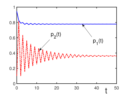
Figure 1: Time dependence of the probabilities $p_{1}(t)$ (solid line) and $p_{2}(t)$ (dash-dotted line), for the initial conditions $f_{1}=0.8$, $q_{1}=0.19$ and $f_{2}=0.9$, $q_{2}=-0.8$, under weak herding effect, with the herding parameters $\varepsilon_{1}=0.05$ and $\varepsilon_{2}=0$. The probabilities tend to the fixed points $p_{1}^{*}=0.778$ and $p_{2}^{*}=0.362$.

2. Under sufficiently strong herding effect the dynamics is smooth and the probabilities are getting closer to each other, as in Fig. 2, where the herding parameters are larger, under the same initial conditions as in Fig. 1.

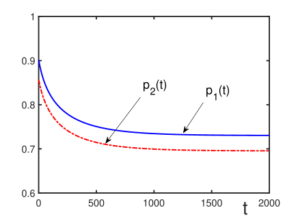
Figure 2: Time dependence of the probabilities $p_{1}(t)$ (solid line) and $p_{2}(t)$ (dash-dotted line), for the same initial conditions, as in Fig.1, with $f_{1}=0.8$, $q_{1}=0.19$ and $f_{2}=0.9$, $q_{2}=-0.8$, but under stronger herding effect, with the herding parameters $\varepsilon_{1}=0.1$ and $\varepsilon_{2}=0.85$. The probabilities tend to the fixed points $p_{1}^{*}=0.730$ and $p_{2}^{*}=0.695$.

3. One of the probabilities tends to a fixed point, while the other at some moment of time starts periodically oscillating and continues oscillating forever, as in Fig. 3.

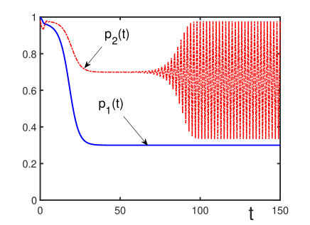
Figure 3: Time dependence of the probabilities $p_{1}(t)$ (solid line) and $p_{2}(t)$ (dash-dotted line), for the initial conditions $f_{1}=0.3$, $q_{1}=0.699$ and $f_{2}=0$, $q_{2}=0.98$, in the absence of herding, with $\varepsilon_{1}=\varepsilon_{2}=0$. The probability $p_{1}(t)$ tends to the fixed points $p_{1}^{*}=0.3$ while $p_{2}(t)$, after a period of smooth behaviour, starts everlasting oscillations.

4. Both probabilities exhibit everlasting periodic oscillations, as in Fig. 4.

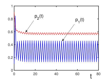
Figure 4: Time dependence of the probabilities $p_{1}(t)$ (solid line) and $p_{2}(t)$ (dash-dotted line), for the initial conditions $f_{1}=0.6$, $q_{1}=0.39$ and $f_{2}=1$, $q_{2}=-0.9$, under strong herding, with the parameters $\varepsilon_{1}=1$ and $\varepsilon_{2}=0.9$. Both probabilities perpetually oscillate.

5. One of the probabilities tends to a fixed point, but the other starts fluctuating chaotically and continues fluctuating for ever, as in Fig. 5.

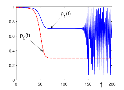
Figure 5: Time dependence of the probabilities $p_{1}(t)$ (solid line) and $p_{2}(t)$ (dash-dotted line), for the initial conditions $f_{1}=0.3$, $q_{1}=0.699$ and $f_{2}=0$, $q_{2}=0.99$, with the herding parameters $\varepsilon_{1}=\varepsilon_{2}=1$. The probability $p_{1}(t)$, after a period of smooth behaviour, suddenly begins chaotically oscillate, while $p_{2}(t)$ monotonically tends to the fixed point $p_{2}^{*}=0.3$.

6. Both probabilities at some moment of time suddenly begin fluctuating chaotically, and keep fluctuating for ever, as in Fig. 6.

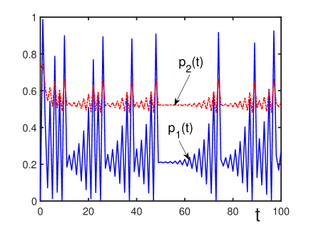
Figure 6: Time dependence of the probabilities $p_{1}(t)$ (solid line) and $p_{2}(t)$ (dash-dotted line), for the initial conditions $f_{1}=0.6$, $q_{1}=0.3$ and $f_{2}=1$, $q_{2}=-0.999$, under the herding parameters $\varepsilon_{1}=1$ and $\varepsilon_{2}=0.8$. Both probabilities exhibit perpetual chaotic oscillations.

The sudden appearance of self-excited periodic and chaotic oscillations is an interesting effect arising in a closed system. The herding behaviour smoothes the trajectories and suppresses both kinds of oscillations, periodic as well as chaotic. The appearance of large oscillations and chaotic fluctuations in decision making can be understood as representing unstable decision making of mentally ill individuals.

5.6 Attenuation of emotion influence

The existence of behavioural paradoxes, considered above, is caused by the presence of emotions of decision makers. The paradoxes arise when subjects make decisions without exchanging information with each other. However, when they are allowed to discuss the problem and to exchange their thoughts, the deviation of the behavioural probabilities from the utility factors diminishes, hence the attraction factors decrease. The paradox attenuation has been confirmed in numerous experimental studies [294, 295, 296, 297, 298, 299, 300, 301, 302, 303, 304].

Thus a series of experiments [304] were accomplished, designed to test whether and to what extent individuals succumb to the conjunction fallacy after discussing the problem with each other. The experimental design of Tversky and Kahneman [255] was used. It was found that, when subjects are allowed to consult between themselves, the proportion of individuals who violate the conjunction principle falls dramatically, especially when the size of the group rises. When individuals are forced to think, they recover in their minds additional information that has been forgotten or shadowed by emotions. The amount of received information increases with the size of the group. As a result, there is a substantially larger drop in the error rate when the group size is increased from two to three than when it is increased from one to two [300, 304]. These experiments confirm the earlier results [298] that there is only a marginal difference between the choices of single individuals and two-person groups, but a significant difference between the choices of two-person and four-person groups in a game. In the experiment by Charness et al. [304] with groups of three members, the fraction of individuals giving the answers deviating from the utility factor dropped to $0.17$. The latter quantity, actually, is the measure of the attraction factor. Thus, after consultations providing additional information, that is after the repeated exchange of information, the attraction factor falls from about $0.25$ to $0.17$. It seems to be natural that, if the discussions and information exchange would continue, the attraction factor would drop further, but it is clear that it should not disappear completely, since the amount of received information is actually never infinite.

The effect of the paradox attenuation, or in other words, the attenuation of the attraction factors after repeated exchange of information, under the conditions discussed above, is illustrated in Fig. 7 and Fig. 8 demonstrating the disjunction effect attenuation. Here the agents of both groups enjoy long-term memory, share the same utility factor, taken as in the experiments of Tversky and Shafir [254] $f_{1}=f_{2}=0.64$, but differ by the initial conditions for the attraction factors. The probabilities $p_{1}(t)$ and $p_{2}(t)$ tend to the consensual limit equal to the utility factor, while the attraction factor, characterizing the paradox, tends to zero, in agreement with the paradox attenuation effect [294, 295, 296, 297, 298, 299, 300, 301, 302, 303, 304]. The tendency of the attraction factors to zero is preserved under different herding parameters.

     

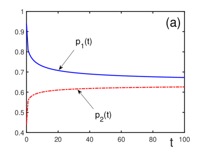
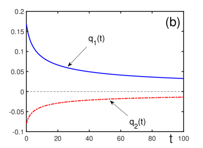
Figure 7: Dynamic disjunction effect. (a) Time dependence of the probabilities $p_{1}(t)$ (solid line) and $p_{2}(t)$ (dash-dotted line) for the initial conditions $f_{1}=f_{2}=0.64$, and $q_{1}=0.3$, $q_{2}=-0.2$, in the absence of herding $\varepsilon_{1}=\varepsilon_{2}=0$. Both probabilities tend to the consensual limit $p_{1}^{*}=p_{2}^{*}=0.64$; (b) Time dependence of the attraction factors $q_{1}(t)$ (solid line) and $q_{2}(t)$ (dash-dotted line) for the same conditions as in Fig.7a. Both attraction factors tend to $q_{1}^{*}=q_{2}^{*}=0$, demonstrating disjunction-effect attenuation.

     

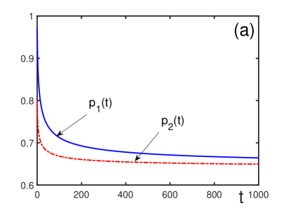
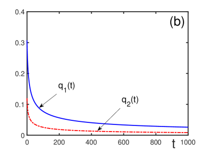
Figure 8: Dynamic disjunction effect. (a) Time dependence of the probabilities $p_{1}(t)$ (solid line) and $p_{2}(t)$ (dash-dotted line) for the initial conditions $f_{1}=f_{2}=0.64$, and $q_{1}=0.35$, $q_{2}=0.15$, for the herding parameters $\varepsilon_{1}=0.1$ and $\varepsilon_{2}=0.05$. Both probabilities tend to the consensual limit $p_{1}^{*}=p_{2}^{*}=0.64$; (b) Time dependence of the attraction factors $q_{1}(t)$ (solid line) and $q_{2}(t)$ (dash-dotted line) for the same conditions as in Fig.8a. Both attraction factors tend to $q_{1}^{*}=q_{2}^{*}=0$, demonstrating disjunction-effect attenuation.

5.7 Continuous decision making

The evolution equations describing the dynamics of preferences deal with multistep decision making, which implies that decisions are taken in discrete moments of time. The temporal interval between subsequent decisions is denoted by $\tau$. If the time of observing the process of taking decisions by decision makers $t$ is much longer than $\tau$, then it seems admissible to expand the probability $p_{j}(A_{n},t+\tau)$ over the small ratio $\tau/t\ll 1$. To first order, this gives

$$p_{j}(A_{n},t+\tau)\simeq p_{j}(A_{n},t)+\frac{\partial p_{j}(A_{n},t)}{\partial t}\;\tau\;.$$ (5.36)

Measuring time in units of $\tau$, we have

$$p_{j}(A_{n},t+1)-p_{j}(A_{n},t)=\frac{\partial p_{j}(A_{n},t)}{\partial t}\;.$$ (5.37)

Then equation (5.5) becomes a differential equation

$$\frac{\partial p_{j}(A_{n},t)}{\partial t}=f_{j}(A_{n},t)+q_{j}(A_{n},t)+h_{j}(A_{n},t)-p_{j}(A_{n},t)\;.$$ (5.38)

Equation (5.38) describes the imaginary process of continuous decision making, assuming that agents can take decisions continuously in time. Of course, such a continuous process sounds not realistic. However, equation (5.38), as it seems, is derived under a reasonable assumption that the observation time is much longer than the time of taking a single decision. It is therefore interesting whether the description of multistep decision making can be done by employing the continuous approximation, that is whether the solutions of the discrete in time equations, characterizing multistep decision making, could be approximated by solutions of continuous in time equation.

The case of two groups deciding on two alternatives, characterized by Eq. (5.34), in the continuous approximation reduces to the equation

$$\frac{dp_{j}(t)}{dt}=f_{j}+q_{j}(t)+h_{j}(t)-p_{j}(t)\;.$$ (5.39)

Substituting here the herding factors (5.30) yields the evolution equations

$$\frac{dp_{1}(t)}{dt}=(1-\varepsilon_{1})[\;f_{1}+q_{1}(t)\;]+\varepsilon_{1}[\;f_{2}+q_{2}(t)\;]-p_{1}(t)\;,$$

$$\frac{dp_{2}(t)}{dt}=(1-\varepsilon_{2})[\;f_{2}+q_{2}(t)\;]+\varepsilon_{2}[\;f_{1}+q_{1}(t)\;]-p_{2}(t)\;,$$ (5.40)

with the attraction factors (5.29). Initial conditions are given by (5.35). If we keep in mind the case of mixed memories, then one group possesses long-term memory (5.31) that, using the Euler-Maclaurin formula, translates into

$$M_{1}(t)=\int_{0}^{t}\mu_{12}(t^{\prime})\;dt^{\prime}+\frac{\mu_{12}(0)+\mu_{12}(t)}{2}\;,$$ (5.41)

while the other group has short-term memory (5.32). For $t=0$, we have

$$M_{1}(0)=\mu_{12}(0)\;,\;M_{2}(0)=\mu_{21}(0)\;.$$ (5.42)

The problem of whether the solutions of time-discrete equations are close to the solutions of their time-continuous approximation is interesting by its own. It is also important for the understanding which of the variants more correctly characterizes real multistep decision making.

5.8 Discrete versus continuous processes

Comparing the solutions to discrete and continuous in time equations (5.34) and (5.40), respectively, it is instructive to compare the solutions for the same parameters and the same initial conditions. As is well known, for two-dimensional dynamical systems, continuous differential equations usually produce more smooth solutions than those of discrete difference equations [305]. This is confirmed by the results of numerical solution of the differential equations (5.40) and their comparison with the solutions of discrete equations (5.34).

Figure 9 demonstrates that the solution to the continuous equation is smooth, and does not display oscillations as the solution to the discrete equation. When the solution to the discrete problem is smooth, then the solution to the continuous problem is also smooth and the related probabilities practically coincide, as it happens for the parameters of Fig. 2, when the solutions of discrete and continuous equations are not distinguishable, because of which we do not repeat them here.

     

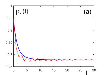
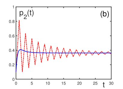
Figure 9: Comparison of the solutions for the probabilities $p_{1}(t)$ and $p_{2}(t)$ for the discrete and continuous decision making. The initial conditions $f_{1}=0.8$, $q_{1}=0.19$ and $f_{2}=0.9$, $q_{2}=-0.8$, under weak herding, with the parameters $\varepsilon_{1}=0.05$ and $\varepsilon_{2}=0$. The probabilities tend to the fixed points $p^{*}_{1}=0.778$ and $p_{2}^{*}=0.362$. (a) Solution $p_{1}(t)$ to continuous equations (solid line), as compared to $p_{1}(t)$ for discrete equations (dash-dotted line); (b) Solution $p_{2}(t)$ to continuous equations (solid line) as compared to $p_{2}(t)$ for discrete equations (dash-dotted line).

If the evolution equations possess fixed points, they are defined by the equations

$$p_{1}^{*}=(1-\varepsilon_{1})(f_{1}+q_{1}^{*})+\varepsilon_{1}(f_{2}+q_{2}^{*})\;,\qquad p_{2}^{*}=(1-\varepsilon_{2})(f_{2}+q_{2}^{*})+\varepsilon_{2}(f_{1}+q_{1}^{*})\;,$$

where $q_{j}^{*}\equiv q_{j}(\infty)$.

Figures 10 and 11 show that the solutions to the continuous equations do not display oscillatory behaviour that exists for discrete equations. And Fig. 12 evidences that the solutions to the continuous equations, as it should be expected, do not possess chaotic behaviour, demonstrated by the discrete equations.

     

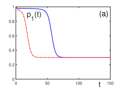
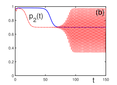
Figure 10: Comparison of the solutions for the probabilities $p_{1}(t)$ and $p_{2}(t)$ for the discrete and continuous decision making. The initial conditions are $f_{1}=0.3$, $q_{1}=0.699$ and $f_{2}=0$, $q_{2}=0.98$, in the absence of herding, with $\varepsilon_{1}=\varepsilon_{2}=0$. (a) Solution $p_{1}(t)$ to continuous equations (solid line), as compared to $p_{1}(t)$ for discrete equations (dash-dotted line). Both probabilities $p_{1}(t)$ tend to the same fixed point $p_{1}^{*}=0.3$; (b) Solution $p_{2}(t)$ to continuous equations (solid line), as compared to $p_{2}(t)$ for discrete equations (dash-dotted line). The continuous solution $p_{2}(t)$ tends to the fixed point $p_{2}^{*}=0.699$, whereas the discrete $p_{2}(t)$, after a period of smooth behaviour, starts periodically oscillating.

     

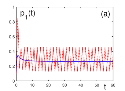
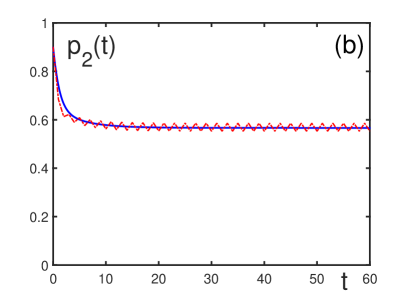
Figure 11: Comparison of the solutions for the probabilities $p_{1}(t)$ and $p_{2}(t)$ for the discrete and continuous decision making. The initial conditions are $f_{1}=0.6$, $q_{1}=0.39$, and $f_{2}=1$, $q_{2}=-0.9$, under strong herding, with the parameters $\varepsilon_{1}=1$ and $\varepsilon_{2}=0.9$. (a) Solution $p_{1}(t)$ to the continuous equations (solid line), as compared to $p_{1}(t)$ for the discrete equations (dash-dotted line). The continuous probability tends to the fixed point $p_{1}^{*}=0.265$, while the discrete probability perpetually oscillates; (b) Solution $p_{2}(t)$ to continuous equations (solid line), as compared to $p_{2}(t)$ for discrete equations (dash-dotted line). The continuous solution $p_{2}(t)$ tends to the fixed point $p_{2}^{*}=0.566$, while the discrete solution $p_{2}(t)$ permanently oscillates.

     

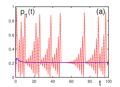
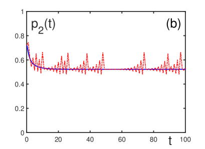
Figure 12: Comparison of the solutions for the probabilities $p_{1}(t)$ and $p_{2}(t)$ for the discrete and continuous decision making. The initial conditions are $f_{1}=0.6$, $q_{1}=0.3$ and $f_{2}=1$, $q_{2}=-0.999$, under the herding parameters $\varepsilon_{1}=1$ and $\varepsilon_{2}=0.8$. (a) Solution $p_{1}(t)$ to the continuous equations (solid line), as compared to $p_{1}(t)$ for the discrete equations (dash-dotted line). The continuous probability tends to the fixed point $p_{1}^{*}=0.210$, while the discrete probability chaotically oscillates; (b) Solution $p_{2}(t)$ to the continuous equations (solid line), as compared to $p_{2}(t)$ for the discrete equations (dash-dotted line). The continuous solution $p_{2}(t)$ tends to the fixed point $p_{2}^{*}=0.522$, while the discrete solution $p_{2}(t)$ chaotically oscillates.

A special case is illustrated in Fig. 13. The solutions $p_{1}(t)$ and $p_{2}(t)$ to the discrete equations sometimes can intersect, as is shown in Fig. 13b. However, the solutions to the continuous equations do not intersect, instead they glue to each other and tend to a common limit, while in the case of the discrete problem, one of the probabilities chaotically oscillates, as is shown in Fig. 14.

     

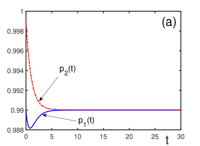
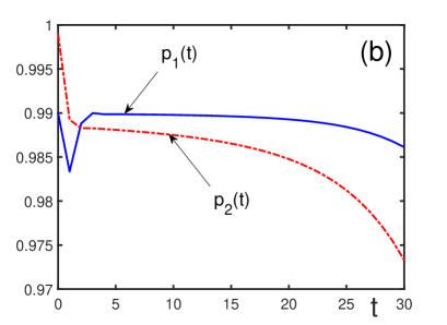
Figure 13: Comparison of the solutions for the probabilities $p_{1}(t)$ (solid line) and $p_{2}(t)$ (dash-dotted line) for the discrete and continuous decision making. The initial conditions are $f_{1}=0.3$, $q_{1}=0.699$ and $f_{2}=0$, $q_{2}=0.99$, with the herding parameters $\varepsilon_{1}=\varepsilon_{2}=1$. (a) Continuous solutions $p_{1}(t)$ (solid line) and $p_{2}(t)$ (dash-dotted line) at the beginning of the process for $t\in[0,30]$; (b) Discrete solutions $p_{1}(t)$ (solid line) and $p_{2}(t)$ (dash-dotted line) at the beginning of the process for $t\in[0,30]$.

     

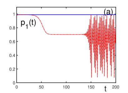
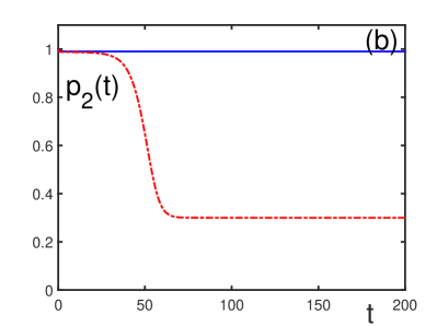
Figure 14: Comparison of the solutions for the probabilities $p_{1}(t)$ and $p_{2}(t)$ for the discrete and continuous decision making. The initial conditions are $f_{1}=0.3$, $q_{1}=0.699$ and $f_{2}=0$, $q_{2}=0.99$, with the herding parameters $\varepsilon_{1}=\varepsilon_{2}=1$. (a) Solution $p_{1}(t)$ to the continuous equations (solid line), as compared to $p_{1}(t)$ for the discrete equations (dash-dotted line). The continuous probability tends to the fixed point $p_{1}^{*}=f_{2}+q_{2}=0.99$, while the discrete probability chaotically oscillates; (b) Solution $p_{2}(t)$ to the continuous equations (solid line), as compared to $p_{2}(t)$ for the discrete equations (dash-dotted line). The continuous probability tends to the fixed point $p_{2}^{*}=f_{2}+q_{2}=0.99$, while the discrete probability tends to $p_{2}^{*}=f_{1}=0.3$.

Thus, the solutions to the continuous equations are always smooth and exhibit neither periodic oscillations nor chaotic fluctuations that exist for the discrete equations. The considered equations describe the process of decision making in a network of intelligent agents. The discrete equations correspond to multistep decision making, as it can be done in real life. The continuous equations serve as an approximation to the studied problem. This approximation is rather accurate when the discrete solutions are smooth. However, the continuous approximation does not catch such interesting cases as periodic oscillations and chaotic fluctuations. These oscillations and fluctuations can arise in realistic problems, where there are the groups of agents with different features, for instance when there occurs the co-existence of agents with different types of memory, say long-term and short-term memory.

5.9 Time discounting of utility

In the dynamical processes of preferences, considered above, the utility factor was treated as a constant quantity. This is a reasonable assumption based on the fact that the period of time when utility does not change is usually much longer than the time of information exchange between the agents of the network. For instance, prices often are not changed during years or at least months, while the information exchange discussing these prices can occur several times a day.

However, in order to have general understanding, let us consider how the utility factors could vary when taking account of time discounting of utility. Then we need to deal with discounted expected utility [282, 306]. In that case, the utility function $u(x)$ for a payoff $x$ is discounted at time $t$ as $D(t)u(x)$. Here $D(t)$ is a discount function with the properties

$$0<D(t)<1\qquad(0<t<\infty)\;,$$

$$D(0)=1\;,\qquad D(\infty)=0\;.$$ (5.43)

A typical example of a discount function is $D(t)=1/(1+r)^{t}$, where $r$ is a discount rate and $t$ is a discrete time counted in some temporal units, usually in units of an year. With the discounted utility functions, the expected utility of a lottery $L_{n}$ becomes discounted as $D(t)U(L_{n})$. Denoting the discounted expected utility of an alternative $A_{n}$ as

$$U(A_{n},t)=U(A_{n})D(t)\;,$$ (5.44)

for the discounted utility factor (3.25), we obtain

$$f(A_{n},t)=\frac{U(A_{n},t)\exp\{\beta U(A_{n},t)\}}{\sum_{n}U(A_{n},t)\exp\{\beta U(A_{n},t)\}}\;.$$ (5.45)

Using here the discounted utility (5.44) gives

$$f(A_{n},t)=\frac{U(A_{n})\exp\{\beta(t)U(A_{n})\}}{\sum_{n}U(A_{n})\exp\{\beta(t)U(A_{n})\}}\;,$$ (5.46)

with the initial expected utilities and the discounted belief function

$$\beta(t)=\beta D(t)$$ (5.47)

enjoying the properties

$$0<\beta(t)<\beta\qquad(0<t<\infty)\;,$$

$$\beta(0)=\beta\;,\qquad\beta(\infty)=0\;.$$ (5.48)

As we see, the utility factor can be considered to be constant if $t\ll 1$, when $\beta(t)\simeq\beta$, if $t\gg 1$, when $\beta(t)\simeq 0$, and also if $\beta\ll 1$, when $\beta(t)\simeq 0$.

In that way, the expected utilities are discounted with time, however they enter the utility factors so that the latter are almost constant for wide time periods, and they do not vary at all for the neutral beliefs of decision makers, when $\beta=0$. Thus the assumption that the utility factor is practically constant has the wide range of applicability.

5.10 Collective network operation

The functioning of a network can be characterized in two ways, by considering the actions of its separate parts and by studying the operation of the network as a whole. Under a network, we can imply a society with the population structured into several different groups or an artificial intelligence consisting of several groups of nodes with different properties. That is, it is possible to study the decision making of parts of a society or the collective decision making by the whole society. Otherwise, it is possible to concentrate on the actions of different parts of a network or on the collective functioning of the whole network.

Suppose, we consider a society (network) of $N$ agents (nodes). The society is structured into $G$ groups (parts) enumerated by $j=1,2,\ldots,G$. Each group is characterized by its specific properties, say its type of memory and herding parameters. The group $j$ consists of $N_{j}$ agents, so that the group $j$ composition fraction is

$$c_{j}\equiv\frac{N_{j}}{N}\qquad(j=1,2,\ldots,G)\;.$$ (5.49)

Hence the normalization conditions are

$$\sum_{j=1}^{G}N_{j}=N\;,\qquad\sum_{j=1}^{G}c_{j}=1\;.$$ (5.50)

As early, the number of agents in a group $j$ choosing an alternative $A_{n}$ at time $t$ is $N_{j}(A_{n},t)$. Since each agent of a group chooses one of the alternatives,

$$\sum_{n=1}^{N_{A}}N_{j}(A_{n},t)=N_{j}\;.$$ (5.51)

The probability that an agent of a group $j$ chooses an alternative $A_{n}$ at time $t$ is

$$p_{j}(A_{n},t)\equiv\frac{N_{j}(A_{n},t)}{N_{j}}\;.$$ (5.52)

The number of agents in the whole society choosing the alternative $A_{n}$ reads as

$$N(A_{n},t)=\sum_{j=1}^{G}N_{j}(A_{n},t)\;.$$ (5.53)

Then the probability that an agent of the whole society chooses an alternative $A_{n}$ at time $t$ is defined as

$$p(A_{n},t)\equiv\frac{N(A_{n},t)}{N}\;.$$ (5.54)

The related normalization condition is

$$\sum_{n=1}^{N_{A}}p(A_{n},t)=1\;.$$ (5.55)

In the above subsections, the temporal behaviour of the group probabilities (5.52) has been investigated. The collective decision of a society, or the collective action of a network is described by the probability (5.54). The group probabilities define the total network probability

$$p(A_{n},t)=\sum_{j=1}^{G}c_{j}p_{j}(A_{n},t)\;,$$ (5.56)

where the structure of the society (network) is prescribed by the given composition fractions $c_{j}$. The collective probability (5.56) characterizes the behaviour of the society (network) as a whole.

6 Conclusion

The review discusses the principal points of how the operation of artificial intelligence has to be organized in order to simulate the so-called human-level artificial intelligence that is able to make decisions taking into account the utility of the considered alternatives as well as emotions accompanying the choice. In order to formalize the operation of such an affective intelligence, it is necessary to characterize the basic rules of human decision making.

First of all, it is required to understand the general structure of affective decision making. The pivotal idea suggesting the main principles of this structure is the formal similarity between decision making under emotions and quantum measurements under intrinsic noise. Cognition-emotion duality in decision making is formally analogous to observable-noise duality in quantum measurements.

It is in no way assumed that the brain is a quantum object or consciousness is in any sense quantum. The analogies between quantum measurements and decision making are purely nominal. It is possible to adduce a number of examples where physically very different processes are characterized by very close mathematics. For instance, many processes of self-organization in complex systems can be interpreted as decision making [201]. As an example of two different in nature phenomena characterized by very similar mathematical description, it is possible to mention that the development and arising distribution of cities over their size can be described as the process of Bose-Einstein condensation [307]. Although the growth of cities and Bose-Einstein condensation, by their nature, are absolutely different processes, they can be described by similar mathematics. In the same vein one has to accept the analogies between quantum measurements and decision making. These analogies turned out to be rather productive suggesting the principal points governing the description of affective decision making.

To be concrete, Sec. 2 presents the general theory of quantum measurements under intrinsic noise. The goal is to analyze what ideas and methods could be accepted for the design of affective decision theory. However, there is no need to involve all that quantum machinery for decision theory because of the following:

(a) From one side, quantum theory is overloaded by numerous notions having no direct meaning in decision theory. Thus, it is not defined what in decision making would be the form of Hamiltonians, of statistical operators, and so on.

(b) From the other side, the notions of quantum theory are not sufficient for suggesting quantitative theory of decision making. This is why the use of quantum techniques for decision making has produced practically no quantitative description and no quantitative predictions. In order to develop a quantitative theory of decision making, one has to complement quantum formulas by quite a number of assumptions of purely classical origin and introduce several fitting parameters.

(c) In addition, involving rather complicated techniques of quantum theory, complementing them by a number of classical assumptions, and equipping with fitting parameters seems to be excessive if a simpler classical description is admissible.

Therefore, borrowing some general ideas from the theory of quantum measurements under intrinsic noise, it looks beneficial to formulate an axiomatic approach to affective decision making in purely classical terms, given in Sec. 3. The ideas of quantum measurement theory serve rather as Ariadne’s thread for formulating affective decision theory that can be used by artificial intelligence. It is in that sense the term “quantum operation of artificial intelligence” is used. The intelligence is not quantum, but its operation imitates some rules specific for quantum theory. The main points borrowed from the theory of noisy measurements are:

1. Decision making has to be treated as a probabilistic process that needs to be characterized by behavioural probabilities defining the fractions of decision makers choosing the related alternatives from a given set.

2. The role of emotions in decision making is similar to the role of intrinsic noise under quantum measurements.

3. Behavioural probability, taking account of cognition-emotion duality, is represented by the superposition of two terms, a rational utility factor, measuring the utility of the alternatives, and an attraction factor, characterizing the role of emotions in the process of decision making. In particular cases, the attraction factor can be split into several terms responsible for different types of emotions.

4. Alternatives and accompanying emotions are entangled in the sense that they are connected with each other and both of them influence the choice.

5. Different types of emotions interfere with each other producing in the behavioural probability the term named attraction factor.

6. It is necessary to distinguish the joint probability of two consecutive events occurring at different moments of time and the joint probability of two events defined as a synchronous probability of two events at different locations. This latter probability, similarly to the probability of a single event, is represented by a sum of utility factor and attraction factor, if emotions are taken into account.

7. Temporal dependence of behavioural probabilities can be modeled by the form arising from the consideration of time dependence of the averages corresponding to observable quantities under non-destructive repeated quantum measurements.

To have predictive power, these principal items can be complemented by non-informative priors characterizing the behaviour of a typical decision maker. All elaboration of affective decision theory can be given in classical terminology, with no quantum formulas explicitly implicated. The behaviour of real decision makers on the aggregate level is quantitatively well described by the formulated affective decision theory, using no fitting parameters. This is confirmed by treating a set of lotteries in Sec. 3.

The famous behavioural paradoxes plaguing classical decision making find their natural resolution in the frame of the affective decision theory taking account of emotions. The paradoxes are not merely qualitatively explained but are in good quantitative agreement with empirical data on the aggregate level, without involving any fitting parameters.

A family of affective intelligent agents composes a network where the agents interact through information exchange. The intelligent agents can differ by their initial conditions and by the type of memory, in the ultimate cases being long-term or short-term memory. There can exist the networks of agents with uniform memory, that is having the same type of memory, but different initial conditions. The most interesting and rich is the behaviour of a mixed network, where a part of agents enjoys long-term memory, while the other part has short-term memory. In these networks there can arise self-excited waves of preferences demonstrating either periodic or chaotic dynamics. Chaotic decision making reminds us the behaviour of patients suffering from mental diseases.

Discussing the multi-step decision making of society agents, we can keep in mind either a human society composed of different groups or a network consisting of several parts of nodes, or the brain composed of neurons.

The described approach, from one side, helps understanding the behaviour of real humans making a choice between alternatives by evaluating their rational utility at the same time being subject to accompanying irrational emotions. From the other side, the formalized rules of the choice followed by a typical decision maker can help for implicating the related algorithms in the operation of a complex Affective Artificial Intelligence.

References

- [1] Nilsson N 1998 Artificial Intelligence: A New Synthesis (San Francisco: Morgan Kaufmann)
- [2] Luger G F and Stubblefield W A 2004 Artificial Intelligence: Structures and Strategies for Complex Problem Solving (Redwood City: Benjamin Cummings)
- [3] Rich E, Knight K and Nair S B 2009 Artificial Intelligence (New Delhi: McGraw Hill)
- [4] Poole D L and Mackworth A K 2017 Artificial Intelligence: Foundations of Computational Agents (Cambridge University Press: Cambridge)
- [5] Neapolitan R E and Jiang X 2018 Artificial Intelligence (New York: Chapman and Hall)
- [6] Russell S J and Norvig P 2021 Artificial Intelligence: A Modern Approach (Pearson: Hoboken)
- [7] Scherer K R and Moors A 2019 The emotion process: Event appraisal and component differentiation Ann. Rev. Psychol. 70 719–745
- [8] Mumenthaler C, Sander D and Manstead A S R 2020 Emotion recognition in simulated social interactions IEEE Trans. Affect. Comput. 11 308–312
- [9] Picard R W 1997 Affective Computing (Cambridge: Massachusetts Institute of Technology)
- [10] Calvo R A, D’Mello S, Cratch J and Kappas A Eds. 2015 The Oxford Handbook of Affective Computing (Oxford: Oxford University Press)
- [11] Lerner J S, Li Y, Valdesolo P, and Kassam K S 2015 Emotion and decision making Annu. Rev. Psychol. 66 799–823
- [12] Zajonc R B 1980 Feeling and thinking: Preferences need no inferences Am. Psychol. 35 151–175
- [13] Zajonc R B 1984 On the primacy of affect Am. Psychol. 39 117–123
- [14] Lazarus R S 1982 Thoughts on the relations between emotion and cognition Am. Psychol. 37 1019–102
- [15] Lazarus R S 1995 Vexing research problems inherent in cognitive-mediational theories of emotion and some solutions Psychol. Inquiry 6 183–196
- [16] Leventhal H and Scherer K 1987 The relationship of emotion to cognition: A functional approach to a semantic controversy Cognit. Emot. 1 3–28
- [17] Pessoa L 2008 On the relationship between emotion and cognition Nature Rev. Neurosci. 9 148–158
- [18] Brosch T, Scherer K R, Grandjean D and Sander D 2013 The impact of emotion on perception, attention, memory, and decision-making Swiss Medic. Weekly 143 13786
- [19] Wentura D 2019 Cognition and emotion: On paradigms and metaphors Cognit. Emot. 33 85–93
- [20] De Houwer J and Hughes S 2019 Toward a cumulative science of emotion: A functional-cognitive framework for emotion research Cognit. Emot. 33 61–66
- [21] Keltner D 2019 Toward a consensual taxonomy of emotions Cognit. Emot. 33 14–19
- [22] Gyurak A, Gross J J and Etkin A 2011 Explicit and implicit emotion regulation: A dual-process framework Cognit. Emot. 25 400–412
- [23] Scherer K 2009 The dynamic architecture of emotion: Evidence for the component process model Cognit. Emot. 23 1307–1351
- [24] Scherer K 2019 Studying appraisal-driven emotion processes: Taking stock and moving to the future Cognit. Emot. 33 31–40
- [25] Koole S L and Rothermund K 2011 I feel better but I don’t know why: The psychology of implicit emotion regulation Cognit. Emot. 25 389–399
- [26] Koole S L and Rothermund K 2019 Revisiting the past and back to the future: Horizons of cognition and emotion research Cognit. Emot. 33 1–7
- [27] Reisenzein R 2019 Cognition and emotion: A plea for theory Cognit. Emot. 33 109–118
- [28] Schwarz N 2000 Emotion, cognition, and decision making Cognit. Emot. 14 433–440
- [29] Ariely D 2008 Predictably Irrational (New York: Harper)
- [30] Bekoff M 2000 Animal Emotions: Exploring Passionate Natures: Current interdisciplinary research provides compelling evidence that many animals experience such emotions as joy, fear, love, despair, and grief–we are not alone Bioscience 50 861–870
- [31] Dittel C, Dufour G, Weihs G and Buchleitner A 2021 Wave-particle duality of many-body quantum states Phys. Rev. X 11 031041
- [32] Bohr N 1933 Light and life. Nature 131 421–423
- [33] Bohr N 1958 Atomic Physics and Human Knowledge (New York: Wiley)
- [34] Khrennikov A Y 2010 Ubiquitous Quantum Structure (Berlin: Springer)
- [35] Busemeyer J R and Bruza P D 2012 Quantum Models of Cognition and Decision (Cambridge: Cambridge University Press)
- [36] Agrawal P M and Sharda R 2013 Quantum mechanics and human decision making Oper. Res. 61 1–16
- [37] Bagarello F 2013 Quantum Dynamics for Classical Systems (Hoboken: Wiley)
- [38] Ashtiani M and Azgomi M A 2015 A survey of quantum-like approaches to decision making and cognition Math. Soc. Sci. 75 49–80
- [39] Wendt A 2015 Quantum Mind and Social Science (Cambridge: Cambridge University Press)
- [40] Penrose R 1989 The Emperor’s New Mind (New York: Oxford University Press)
- [41] Hameroff S 1994 Quantum coherence in microtubules: A neural basis for emergent consciousness J. Consc. Stud. 1 91–118
- [42] Tegmark M 2000 Importance of quantum decoherence in brain processes Phys. Rev. E 61 4194–4205
- [43] Al-Khalili J and McFadden J 2014 Life on the Edge: The Coming of Age of Quantum Biology (London: Bantam Press)
- [44] Jedlicka P 2017 Revisiting the quantum brain hypothesis: Toward quantum (Neuro)biology? Front. Mol. Neurosci. 10 366
- [45] Boyer-Kassem T, Duchêne S and Guerci E 2016 Testing quantum-like models of judgment for question order effect Math. Soc. Sci. 80 33–46
- [46] Boyer-Kassem T, Duchêne S and Guerci E 2016 Quantum-like models cannot account for the conjunction fallacy Theory Decis. 81 479–510
- [47] Zheltikov A M 2017 The critique of quantum mind: Measurement, consciousness, delayed choice, and lost coherence Phys. Usp. 61 1016–1025
- [48] Dakic B, Suvakov M, Paterek T and Brukner C 2008 Efficient hidden-variable simulation of measurements in quantum experiment Phys. Rev. Lett. 101 190402
- [49] Sober E 2015 Ockam’s Razor: A User’s Manual (Cambridge: Cambridge University Press)
- [50] von Neumann J 1955 Mathematical Foundations of Quantum Mechanics (Princeton: Princeton University Press)
- [51] Benioff P A 1972 Decision procedures in quantum mechanics J. Math. Phys. 13 908–914
- [52] Benioff P A 1972 Procedures in quantum mechanics without Von Neumann’s projection axiom J. Math. Phys. 13 1347–1354
- [53] Wellens T, Shatokhin V and Buchleitner A 2004 Stochastic resonance Rep. Prog. Phys. 67 45–105
- [54] Gardiner C W and Zoller P 2004 Quantum Noise (Berlin: Springer)
- [55] Horsthemke W and Lefever R 1984 Noise-Induced Transitions (Berlin: Springer)
- [56] Gardiner C W 1985 Handbook of Stochastic Methods (Berlin: Springer)
- [57] Yukalov V I 2021 Tossing quantum coins and dice Laser Phys. 31 055201
- [58] Yukalov V I and Sornette D 2008 Quantum decision theory as quantum theory of measurement Phys. Lett. A 372 6867–6871
- [59] Yukalov V I and Sornette D 2009 Scheme of thinking quantum systems Laser Phys. Lett. 6 833–839
- [60] Yukalov V I and Sornette D 2009 Processing information in quantum decision theory Entropy 11 1073–1120
- [61] Yukalov V I 2022 Quantum uncertainty in decision theory Stud. Syst. Decis. Contr. 427 201–218
- [62] Birkhoff G and von Neumann J 1936 The logic of quantum mechanics Ann. Math. 37 823–843
- [63] Hughes R L 1981 Quantum logic Sci. Am. 245 146–157
- [64] Holevo A S 1973 Statistical decision theory for quantum systems J. Multivar. Anal. 3 337–394
- [65] Holevo A 2011 Probabilistic and Statistical Aspects of Quantum Theory (Berlin: Springer)
- [66] Dirac P A M 1939 A new notation for quantum mechanics Math. Proc. Cambridge Philos. Soc. 35 416–418
- [67] Bogolubov N N 1967 Lectures on Quantum Statistics vol. 1 (New York: Gordon and Breach)
- [68] Bogolubov N N 1970 Lectures on Quantum Statistics vol. 2 (New York: Gordon and Breach)
- [69] Bogolubov N N 2015 Quantum Statistical Mechanics (Singapore: World Scientific)
- [70] Yukalov V I and Sornette D 2016 Quantum probability and quantum decision making Philos. Trans. Roy. Soc. A 374 20150100
- [71] Yukalov V I and Sornette D 2015 Quantum theory of measurements as quantum decision theory J. Phys. Conf. Ser. 594 012048
- [72] Buchleitner A and Hornberger K Eds. Coherent Evolution in Noisy Environments (Berlin: Springer)
- [73] Yukalov V I 2020 Evolutionary processes in quantum decision theory Entropy 22 681
- [74] Yukalov V I and Sornette D 2015 Positive operator-valued measures in quantum decision making Lect. Notes Comput. Sci. 8951 146–161
- [75] Conway J 1990 A Course in Functional Analysis (Berlin: Springer)
- [76] Yukalov V I 2013 Theory of cold atoms: Basics of quantum statistics Laser Phys. 23 062001
- [77] Zurek W H 2003 Decoherence, einselection, and the quantum origins of the classical Rev. Mod. Phys. 75 715–776
- [78] Schlosshauer M 2005 Decoherence, the measurement problem, and interpretations of quantum mechanics Rev. Mod. Phys. 76 1267–1305
- [79] Yukalov V I and Sornette D 2014 Manipulating decision making of typical agents IEEE Trans. Syst. Man Cybern. Syst. 44 1155–1168
- [80] Yukalov V I and Sornette D 2010 Mathematical structure of quantum decision theory Adv. Compl. Syst. 13 659–698
- [81] Yukalov V I and Sornette D 2014 How brains make decisions Springer Proc. Phys. 150 37–53
- [82] Vedral V 2006 Introduction to Quantum Information Science (Oxford: Oxford University Press)
- [83] Yukalov V I and Sornette D 2013 Quantum probabilities of composite events in quantum measurements with multimode states Laser Phys. 23 105502
- [84] Yukalov V I, Yukalova E P and Sornette D 2013 Mode interference in quantum joint probabilities for multimode Bose-condensed systems Laser Phys. Lett. 10 115502
- [85] Yukalov V I and Sornette D 2014 Conditions for quantum interference in cognitive sciences. Top. Cogn. Sci. 6 79–90
- [86] Griffiths D J 2017 Introduction to Quantum Mechanics (Cambridge: Cambridge University Press)
- [87] Williams C P and Clearwater S H 1998 Explorations in Quantum Computing (New York: Springer)
- [88] Nielsen M A and Chuang I L 2000 Quantum Computation and Quantum Information (Cambridge: Cambridge University Press)
- [89] Vedral V 2002 The role of relative entropy in quantum information theory Rev. Mod. Phys. 74 197–234
- [90] Keyl M 2002 Fundamentals of quantum information theory, Phys. Rep. 369 431–548
- [91] Mintert F, de Carvalho A R R, Kus M and Buchleitner A 2005 Measures and dynamics of entangled states Phys. Rep. 415 207–259
- [92] Gühne O and Toth G 2009 Entanglement detection Phys. Rep. 474 1–75
- [93] Wilde M 2013 Quantum Information Theory (Cambridge: Cambridge University Press)
- [94] Yukalov V I and Sornette D 2011 Decision theory with prospect interference and entanglement Theory Decis. 70 283–328
- [95] Yukalov V I and Sornette D 2014 Quantum probabilities and entanglement for multimode quantum systems J. Phys. Conf. Ser. 497 012034
- [96] Marcus M D and Moyls B N 1959 Transformations on tensor product spaces Pacif. J. Math. 9 1215–1221
- [97] Westwick R 1967 Transformations on tensor spaces Pacif. J. Math. 23 613–620
- [98] Johnston N 2011 Characterizing operations preserving separability measures via linear preserver problems Linear Multilin. Algebra 59 1171–1187
- [99] Beasley L 1988 Linear operators on matrices: The invariance of rank- matrices Linear Algebra Appl. 107 161–167
- [100] Alfsen E and Shultz F 2010 Unique decompositions, faces, and automorphisms of separable states J. Math. Phys. 51 05220
- [101] Friedland S, Li C K, Poon Y T and Sze N S 2011 The automorphism group of separable states in quantum information theory J. Math. Phys. 52 042203
- [102] Gohberg J and Goldberg S 1987 Semi-separable operators along chains of projections and systems J. Math. Anal. Appl. 125 124–140
- [103] Crouzeux J P and Hassouni A 1994 Quasimonotonicity of separable operators and monotonicity indices SIAM J. Optim. 4 649–658
- [104] Fan H Y 2001 Normally ordered expansions of entangling operators and their squeezing transformation Mod. Phys. Lett. B 15 1475–1483
- [105] Dao-Ming L 2016 Fundamental entangling operators in quantum mechanics and their properties Int. J. Theor. Phys. 55 3156–3163
- [106] Chen J, Duan R, Ji Z, Ying M and Yu J 2008 Existence of universal entangler J. Math. Phys. 49 012103
- [107] Yukalov V I 2003 Entanglement measure for composite systems Phys. Rev. Lett. 90 167905
- [108] Yukalov V I 2003 Quantifying entanglement production of quantum operations Phys. Rev. A 68 022109
- [109] Yukalov V I 2003 Evolutional entanglement in nonequilibrium processes Mod. Phys. Lett. B 17 95–103
- [110] Yukalov V I and Yukalova E P 2006 Entanglement production with multimode Bose-Einstein condensates in optical lattices Laser Phys. 16 354–359
- [111] Yukalov V I and Yukalova E P 2006 Regulating entanglement production in multitrap Bose-Einstein condensates Phys. Rev. A 73 022335
- [112] Yukalov V I 2004 Entanglement production under collective radiation Laser Phys. 14 1403–1414
- [113] Yukalov V I and Yukalova E P 2015 Evolutional entanglement production Phys. Rev. A 92 052121
- [114] Yukalov V I 2020 Order indices and entanglement production in quantum systems Entropy 22 565
- [115] Yukalov V I and Sornette D 2010 Entanglement production in quantum decision theory Phys. At. Nucl. 73 559–562.
- [116] Lüders G 1951 Concerning the state change due to the measurement process Ann. Phys. (Berlin) 8 322–328
- [117] Balian R 1989 On the principles of quantum mechanics and the reduction of the wave packet Am. J. Phys. 57 1019–1027
- [118] Goodman I R, Nguyen H T and, Walker E A 1991 Conditional Inference and Logic for Intelligent Systems (Amsterdam: North-Holland)
- [119] Kolmogorov A N 1956 Foundations of the Theory of Probability (New York: Chelsea)
- [120] Pashle H Dual-task interference in simple tasks: Data and theory Psychol. Bull. 116 220–244
- [121] Cowan N 2010 Multiple concurrent thoughts: The meaning and developmental neuropsychology of working memory. Dev. Neuropsychol. 35 447–474
- [122] Goldstein E B 2015 Cognitive Psychology: Connecting Mind, Research And Everyday Experience (Boston: Cengage Learning)
- [123] Yukalov V I 1970 Existence of a wave function for a subsystem Moscow Univ. Phys. Bull. 25 68–73
- [124] Yukalov V I 2002 Stochastic instability of quasi-isolated systems Phys. Rev. E 65 056118
- [125] Yukalov V I 2003 Irreversibility of time for quasi-isolated systems Phys. Lett. A 308 313–318
- [126] Yukalov V I and Sornette D 2016 Inconclusive quantum measurements and decisions under uncertainty Front. Phys. 4 12
- [127] Yukalov V I and Sornette D 2018 Quantitative predictions in quantum decision theory IEEE Trans. Syst. Man Cybern. Syst. 48 366–381
- [128] Darwin C 1872 The Expression of the Emotions in Man and Animals (New York: Filiquarian)
- [129] Hess U and Thibault P 2009 Darwin and emotion expression Am. Psychol. 64 120–128
- [130] Mirabella G 2018 The weight of emotions in decision-making: How fearful and happy facial stimuli modulate action readiness of goal-directed actions Front. Psychol. 9 1334
- [131] Garcia-Garcia M, Yordanova J, Kolev V, Dominguez-Borras J, and Escera C 2010 Tuning the brain for novelty detection under emotional threat: The role of increasing gamma-phase synchronization Neuro Image 49 1038–1044
- [132] Garcia-Garcia M 2020 The Role of Emotions in Human Decision Making (Paris: Global Lead of Neuroscience)
- [133] Endelberg S and Bendelac Y 2004 Measurement of physical constants using noise IEEE Instrum. Measur. Mag. 6 49–52
- [134] McDonnell M D and Ward L M 2011 The benefits of noise in neural systems: Bridging theory and experiment Nature Rev. Neurosci. 12 415–425
- [135] von Neumann J and Morgenstern O 1953 Theory of Games and Economic Behavior (Princeton: Princeton University Press)
- [136] Savage L J 1954 The Foundations of Statistics (New York: Wiley)
- [137] Arrow K J 1971 Essays in the Theory of Risk Bearing (Chicago: Markham)
- [138] Pratt J W 1964 Risk aversion in the small and in the large Econometrica 32 122–136
- [139] Rothschild M and Stiglitz J 1970 Increasing risk: A definition J. Econ. Theory 2 225–243
- [140] Rothschild M and Stiglitz J 1971 Increasing risk: Its economic consequences J. Econ. Theory 3 66–84
- [141] Friedman M and Savage L 1948 The utility analysis of choices involving risk J. Polit. Econ. 56 279–304
- [142] Markowitz H 1952 The utility of wealth J. Polit. Econ. 60 151–158
- [143] Allais M 1953 Le comportement de l’homme rationnel devant le risque: Critique des postulats et axiomes de l’ecole Americaine Econometrica 21 503–546
- [144] Edwards W 1955 The prediction of decision among bets J. Exp. Psychol. 50 200–204
- [145] Edwards W 1962 Subjective probabilities inferred from decisions Psychol. Rev. 69 109–135
- [146] Ellsberg D 1961 Risk, ambiguity, and the Savage axioms Quart. J. Econ. 75 643–669
- [147] Slovic P and Tversky A 1974 Who accepts Savage axioms? Behav. Sci. 19 368–373.
- [148] Camerer C F, Loewenstein G and Rabin R, Eds. 2003 Advances in Behavioral Economics (Princeton: Princeton University Press)
- [149] Miljkovic D 2005 Rational choice and irrational individuals or simply an irrational theory: A critical review of the hypothesis of perfect rationality J. Socio-Econ. 34 621–634
- [150] Machina M J 2008 Non-expected utility theory in: New Palgrave Dictionary of Economics Eds. Durlauf S N and Blume L E 2008 (New York: Macmillan)
- [151] Kahneman D and Tversky A 1979 Prospect theory: An analysis of decision under risk Econometrica 47 263–292
- [152] Tversky A and Kahneman D 1992 Advances in prospect theory: Cumulative representations of uncertainty J. Risk Uncert. 5 297–323
- [153] Karmarkar U 1978 Subjectively weighted utility: A descriptive extension of the expected utility model Org. Behav. Human Perform. 21 61–72
- [154] Karmarkar U 1979 Subjectively weighted utility and the Allais paradox Org. Behav. Human Perform. 24 67–72
- [155] Chew S 1983 A generalization of the quasilinear mean with applications to the measurement of income inequality and decision theory resolving the Allais paradox Econometrica 51 1065–1092
- [156] Loomes G and Sugden R 1982 Regret theory: An alternative theory of rational choice under uncertainty Econ. J. 92 805–824
- [157] Hey J 1984 The economics of optimism and pessimism: A definition and some applications Kyklos 37 181–205
- [158] Green J and Jullien B 1988 Ordinal independence in nonlinear utility theory J. Risk Uncert. 1 355–387
- [159] Chew S, Epstein L and Segal U 1991 Mixture symmetry and quadratic utility Econometrica 59 139–163
- [160] Pandey M 2018 The opportunity-threat theory of decision-making under risk Judg. Decis. Mak. 13 33–41
- [161] Hill B 2019 A non-Bayesian theory of state-dependent utility Econometrica 87 1341–1366
- [162] Safra Z and Segal U 2008 Calibration results for non-expected utility theories Econometrica 76 1143–1166
- [163] Birnbaum M H 2008 New paradoxes of risky decision making Psychol. Rev. 115 463–501
- [164] Al-Najjar N I and Weinstein J 2009 The ambiguity aversion literature: A critical assessment Econ. Philos. 25 249–284
- [165] Al-Najjar N I and Weinstein J 2009 The ambiguity aversion literature: A critical assessment Econ. Philos. 25 357–369.
- [166] Sun R 2002 Duality of the Mind (Mahwah: Lawrence Erlbaum Associates)
- [167] Paivio A 2007 Mind and Its Evolution: A Dual Coding Theoretical Approach (Mahwah: Lawrence Erlbaum Associates)
- [168] Evans J 2007 Dual-processing accounts of reasoning, judgment, and social cognition Annu. Rev. Psychol. 59 268–269
- [169] Stanovich K E 2011 Rationality and the Reflective Mind (New York: Oxford University Press)
- [170] Kahneman D 2012 Thinking, Fast and Slow (New York: Farrar, Straus and Giroux)
- [171] Zafirovski M 2012 Beneath rational choice: Elements of irrational choice theory Current Sociol. 61 3–21
- [172] Bialek M and De Neys W 2017 Dual processes and moral conflict: Evidence for deontological reasoner’s intuitive utilitarian sensitivity Judg. Decis. Mak. 12 148–167
- [173] Gurcay B and Baron J 2017 Challenges for the sequential two-system model of moral judgement Think. Reason. 23 49–80
- [174] Vaisey S 2009 Motivation and justification: A dual-process model of culture in action Am. J. Sociol. 114 1675–1715
- [175] Evans J 2012 Questions and challenges for the new psychology of reasoning Think. Reason. 18 5–31
- [176] Evans J and Stanovich K E 2013 Dual-process theories of higher cognition: Advancing the debate Perspect. Psychol. Sci. 8 223–241
- [177] Goel V, Buchel C, Frith C and, Dolan R J 2000 Dissociation of mechanisms underlying syllogistic reasoning Neuro Image 12 504–514
- [178] Goel V and Dolan R J 2003 Explaining modulation of reasoning by belief Cognition 87 B11–B22
- [179] Libert B 2006 Reflections on the interaction of the mind and brain Prog. Neurobiol. 78 322–326
- [180] Milner A D and Goodale M A 2008 Two visual systems re-viewed Neuropsychologia 46 774–785
- [181] Tsujii T and Watanabe S 2009 Neural correlates of dual-task effect on belief-bias syllogistic reasoning: A near-infrared spectroscopy study Brain Res. 1287 118–125
- [182] Werner G and Mountcastle V B 1963 The variability of central neural activity in a sensory system and its implications for the central reflection of sensory events J. Neurophysiol. 26 958–977
- [183] Arieli A, Sterkin A, Grinvald A and, Aertsen A 1986 Dynamics of ongoing activity: Explanation of the large variability in evoked cortical responses Science 273 1868–1871
- [184] Gold J I and Shadlen M N 2001 Neural computations that underlie decisions about sensory stimuli Trends Cognit. Sci. 5 10–16
- [185] Glimcher P W 2005 Indeterminacy in brain and behaviour Annu. Rev. Psychol. 56 25–56
- [186] Schumacher J F, Thompson S K and Olman C A 2011 Contrast response functions for single Gabor patches: ROI-based analysis over-represents low-contrast patches for GE BOLD Front. Syst. Neurosci. 5 1–10
- [187] Shadlen M N and Shohamy D 2016 Perspective decision making and sequential sampling from memory Neuron 90 927–939
- [188] Webb R 2019 The neural dynamics of stochastic choice Manag. Sci. 65 230–255
- [189] Kurtz-David V, Persitz D, Webb R and Levy D J 2019 The neural computation of inconsistent choice behaviour Nature Commun. 10 1583
- [190] Woodford M 2020 Modeling imprecision in perception, valuation, and choice Annu. Rev. Econ. 12 579–601
- [191] Yaari M E 1987 The dual theory of choice under risk Econometrica 55 95–115
- [192] Reynaa V F and Brainer C J 2011 Dual processes in decision making and developmental neuroscience: A fuzzy-trace model Developm. Rev. 31 180–206
- [193] Yukalov V I 2022 Quantification of emotions in decision making Soft Comput. 26 2419–2436
- [194] McFadden D 1976 Quantal choice analysis: A surevey Ann. Econ. Soc. Measur. 5 363–390
- [195] Hensher D, Rose J and Greene W 2005 Applied Choice Analysis: A Primer (Cambridge: Cambridge University Press)
- [196] Train K 2009 D͡iscrete Choice Methods with Simulation (Cambridge: Cambridge University Press)
- [197] Schmeidler D 1989 Subjective probability and expected utility without additivity Econometrica 57 571–587
- [198] Gilboa I and Schmeidler D 1993 Updating ambiguous beliefs J. Econ. Theory 59 33–49
- [199] Viscusi W K and Evans W N 2006 Behavioural probabilities J. Risk Uncert. 32 5–15
- [200] Yukalov V I and Sornette D 2017, Quantum probabilities as behavioral probabilities Entropy 19 112
- [201] Yukalov V I and Sornette D 2014 Self-organization in complex systems as decision making Adv. Compl. Syst. 17 1450016
- [202] Yukalov V I and Sornette D 2015 Role of information in decision making of social agents Int. J. Inf. Technol. Decis. Mak. 14 1129–1166
- [203] Kullback S and Leibler R A 1951 On information and sufficiency Ann. Math. Stat. 22 79–86
- [204] Kullback S 1959 Information Theory and Statistics (New York: Wiley)
- [205] Shore J and Johnson R 1980 Axiomatic derivation of the principle of maximum entropy and the principle of minimum cross-entropy IEEE Trans. Inform. Theory 26 26–37
- [206] Luce R D 1959 Individual Choice Behavior: A Theoretical Analysis (New York: Wiley)
- [207] Luce R D and Raiffa R 1989 Games and Decisions: Introduction and Critical Survey (New York: Dover)
- [208] Gul F, Natenzon P and Pesendorfer W 2104 Random choice as behavioral optimization Econometrica 82 1873–1912
- [209] Yukalov V I and Sornette D 2015 Preference reversal in quantum decision theory Front. Psychol. 6 1538
- [210] Epstein L G 1999 A definition of uncertainty aversion Rev. Econ. Stud. 66 579–608
- [211] Camerer C 2003 Behavioral Game Theory (Princeton: Princeton University Press)
- [212] Tversky A 2004 Preference, Belief, and Similarity: Selected Writings (Cambridge: Massachusetts Institute of Technology)
- [213] Tomasello M 2009 Why We Cooperate (Cambridge: Massachusetts Institute of Technology)
- [214] Tomasello M, Melis A P, Tennie C, Wyman E and Herrmann E 2012 Two key steps in the evolution of human cooperation Current Anthropol. 53 673–692
- [215] Perc M, Gómez-Gardeñes J, Szolnoki A, Floria L M and Moreno Y 2013 Evolutionary dynamics of group interactions on structured populations: A review J. Roy. Soc. Interface 10 20120997
- [216] Perc M, Jordan J J, Rand D J, Wang Z, Boccaletti S and Szolnoki A 2017 Statistical physics of human cooperation Phys. Rep. 687 1–51
- [217] Jusup M, Holme P, Kanazawa K, Takayasu M, Romic I, Wang Z, Gecek S, Lipic T, Podobnik B, Wang L, Luo W, Klanjscek T, Fan J, Boccaletti S and Perc M 2022 Social physics Phys. Rep. 948 1–148
- [218] Favre M, Wittwer A, Heinimann H R, Yukalov V I and Sornette D 2016 Quantum decision theory in simple risky choices PLOS One 11 0168045
- [219] Murphy R O and ten Brincke R H W 2018 Hierarchical maximum likelihood parameter estimation for cumulative prospect theory: Improving the reliability of individual risk parameter estimates Manag. Sci. 64 308–326
- [220] Kovalenko T, Vincent S, Yukalov V I and Sornette D 2023 Calibration of quantum decision theory: Aversion to large losses and predictability of probabilistic choices J. Phys. Complex. 4 015009
- [221] Ferro G M, Kovalenko T and Sornette D 2021 Quantum decision theory augments rank-dependent expected utility and cumulative prospect theory J. Econ. Psychol. 86 102417
- [222] Quiggin J 1982 A theory of anticipated utility J. Econ. Behav. Org. 3 323–343
- [223] Zhang C and Kjellström H 2021 A subjective model of human decision making based on quantum decision theory arXiv: 2101.05851
- [224] Tversky A and Kahneman D 1981 The framing of decisions and the psychology of choice Science 211 453–458
- [225] Diederich A, Wyszynski M and Traub S 2020 Need, frames, and time constraints in risky decision-making Theory Decis. 89 1–37
- [226] Siegel S 1957 Level of aspiration and decision making Psychol. Rev. 64 253–262
- [227] Ho T K 1998 The random subspace method for constructing decision forests IEEE Trans. Pattern Anal. Machine Intell. 20 832–844
- [228] Chen T and Guestrin C 2016 XGBoost: A Scalable Tree Boosting System Proc. Int. Conf. Knowl. Discov. Data Mining pp 785–792 Eds. Krishnapuram B et al. (San Francisco: ACM)
- [229] Jain A K, Mao J and Mohiuddin K M 1996 Artificial neural networks: A tutorial Computer 29 31–44
- [230] Kane R 2005 A Contemporary Introduction to Free Will (New York: Oxford University Press)
- [231] Kim B E, Seligman D and Kable J M 2012 Preference reversals in decision making under risk are accompanied by changes in attention to different attributes Front. Neurosci. 6 109
- [232] Hillson D 2003 Effective Opportunity Management for Projects (New York: Marcel Dekker)
- [233] Hillson D 2019 Capturing Upside Risk (Boca Raton: CRC Press)
- [234] Rabin M 2000 Risk aversion and expected-utility theory: A calibration theorem Econometrica 68 1281–1292
- [235] Cohen J and Cohen P 1983 Applied Multiple Regression/Correlation Analysis for Behavioral Sciences (Hillsdale: Erlbaum)
- [236] Payne J W, Bettman J R and Johnson E J 1993 The Adaptive Decision Maker (Cambridge: Cambridge University Press)
- [237] Jedlicka P 2017 Revisiting the quantum brain hypothesis: Toward quantum neurobiology Front. Mol. Neurosci. 10 366
- [238] Bernoulli D 1738 Exposition of a new theory on the measurement of risk Proc. Imp. Acad. Sci. St. Petersburg 5 175–192
- [239] Martin R M 2008 The St. Petersburg paradox in: Stanford Encyclopedia of Philosophy (Stanford: Stanford University Press)
- [240] Yukalov V I 2021 A resolution of St. Petersburg paradox J. Math. Econ. 97 102537
- [241] Samuelson P A 1960 The St. Petersburg paradox as a divergent double limit Int. Econ. Rev. 1 31–37
- [242] Samuelson P A 1977 St. Petersburg paradoxes: Defanged, dissected, and historically described J. Econ. Lit. 15 24–55
- [243] Cox J C, Sadiraj V and Vogt B 2009 On the empirical relevance of St. Petersburg lotteries Econ. Bull. 29 214–220
- [244] Hayden B Y and Platt M L 2009 The mean, the median, and the St. Petersburg paradox Judg. Decis. Mak. 4 256–272
- [245] Neugebauer T 2010 Moral impossibility in the St. Petersburg paradox: A literature survey and experimental evidence Luxembourg School of Finance Preprint
- [246] Cox J C, Kroll M, Lichters V, Sadiraj E B and Vogt B 2018 The St. Petersburg paradox despite risk-seeking preferences: An experimental study Busin. Res. 12 27–44
- [247] Nobandegani A S and Shultz T R 2020 The St. Petersburg paradox: A fresh algorithmic perspective Association for the Advancement of Artificial Intelligence Preprint
- [248] Aloysius J A 2003 Rational escalation of costs by playing a sequence of unfavorable gambles: The martingale J. Econ. Behav. Organ. 51 111–129
- [249] Machina M J 1987 Choice under uncertainty: Problems solved and unsolved Econ. Perspect. 1 121–154
- [250] Machina M J 2009 Risk, ambiguity, and the rank-dependence axioms Am. Econ. Rev. 99 385–392
- [251] Machina M J 2014 Ambiguity aversion with three or more outcomes Am. Econ. Rev. 104 3814–3840
- [252] Poundstone W 1992 Prisoner’s Dilemma (New York: Doubleday)
- [253] Kaminski M 2004 Games Prisoners Play (Princeton: Princeton University Press)
- [254] Tversky A and Shafir E 1992 The disjunction effect in choice under uncertainty Psychol. Sci. 3 305–310
- [255] Tversky A and Kahneman D 1983 Extensional versus intuitive reasoning: The conjunction fallacy in probability judgement Psychol. Rev. 90 293–315
- [256] Shafir E B, Smith E E and Osherson D N 1990 Typicality and reasoning fallacies Memory Cognit. 18 229–239
- [257] Kovalenko T and Sornette D 2022 The conjunction fallacy in quantum decision theory Stud. Syst. Decis. Contr. 429 127–183
- [258] Shefrin H and Statman M 1985 The disposition to sell winners too early and ride losers too long: Theory and evidence J. Finance 40 777–790
- [259] Weber M and Camerer C 1995 The disposition effect in securities trading: An experimental analysis J. Econ. Behav. Org. 33 167–184
- [260] Huber J, Payne J W and Puto C Adding asymmetrically dominated alternatives: Violations of regularity and similarity hypothesis J. Consum. Res. 9 90–98
- [261] Simonson I 1989 Choice based on reasons: The case of attraction and compromise effects J. Consum. Res. 16 158–174
- [262] Wedell D H Distinguishing among models of contextuality induced preference reversals Learn. Memory Cogn. 17 767–778
- [263] Tversky A and Simonson I 1993 Context-dependent preferences Manag. Sci. 39 1179–1189
- [264] Ariely D and Wallsten T S 1995 Seeking subjective dominance in multidimensional space: An explanation of the asymmetric dominance effect Org. Behav. Human Decis. Process. 63 223–232
- [265] Bateson M and Healy S D 2006 Comparative evaluation and its implications for mate choice Trends Ecol. Evol. 20 659–664
- [266] Lea A M and Ryan M J 2015 Irrationality in mate choice revealed by tungara frogs Science 349 964–966
- [267] Benfari R C and Ockene J K 1982 Control of cigarette smoking from a psychological perspective Ann. Rev. Public Health 3 101–128
- [268] Westmaas J L 2010 Social support in smoking cessation: Reconciling theory and evidence Nicotine Tobacco Res. 12 695–707
- [269] Yukalov V I and Sornette D 2009 Physics of risk and uncertainty in quantum decision making Eur. Phys. J. B 71 533–548
- [270] Tversky A and Thaler R H 1990 Anomalies: Preference reversals J. Econ. Persp. 4 201–211
- [271] Tversky A 1969 Intransitivity of preferences Psychol. Rev. 76 31–48
- [272] Fishburn P C and LaValle I H 1988 Context-dependent choice with nonlinear and nontransitive preferences Econometrica 56 1221–1239
- [273] Fishburn P C 1991 Nontransitive preferences in decision theory J. Risk Uncert. 4 113–134
- [274] Panda S C 2018 Rational choice with intransitive preferences Stud. Microecon. 6 66–83
- [275] Tsetsos K, Moran R, Moreland J, Chater N, Uscher M and Summerfield C 2016 Economic irrationality is optimal during noisy decision making Proc. Natl. Acad. Sci. USA 113 3102–3107
- [276] Shaughnessy J J, Zechmeister E B and Zechmeister J S 2006 Research Methods in Psychology (New York: McGraw-Hill)
- [277] Teichert T, Grinband J and Ferrera V 2016 The importance of decision onset J. Neurophysiol. 115 643–661
- [278] Hochman G, Ayal S and Glöckner A 2010 Physiological arousal in processing recognition information: Ignoring or integrating cognitive cues? Judg. Decis. Mak. 5 285–299
- [279] Yukalov V I, Yukalova E P and Sornette D 2018 Information processing by networks of quantum decision makers Physica A 492 747–766
- [280] Yukalov V I, Yukalova E P and Sornette D 2022 Role of collective information in networks of quantum operating agents Physica A 598 127365
- [281] Yukalov V I and Yukalova E P 2022 Self-excited waves in complex social systems Physica D 433 133188
- [282] Frederick S, Loewenstein G and O’Donoghue T 2002 Time discounting and time preference: A critical review J. Econ. Liter. 40 351–401
- [283] Yukalov V I 2011 Equilibration and thermalization in finite quantum systems Laser Phys. Lett. 8 485–507
- [284] Yukalov V I 2012 Equilibration of quasi-isolated quantum systems Phys. Lett. A 376 550–554
- [285] Yukalov V I 2012 Decoherence and equilibration under nondestructive measurements Ann. Phys. (N.Y.) 327 253–263
- [286] Martin E D 1920 The Behavior of Crowds: A Psychological Study (New York: Harper)
- [287] Sherif M 1936 The Psychology of Social Norms (New York: Harper Collins)
- [288] Smelser N J 1963 Theory of Collective Behavior (Glencoe: Free Press)
- [289] Merton R K 1968 Social Theory and Social Structure (New York: Free Press)
- [290] Turner R H and Killian L M 1993 Collective Behavior (Englewood Cliffs: Prentice-Hall)
- [291] Hatfield E, Cacioppo J T and Rapson R L 1994 Emotional Contagion (New York: Cambridge University Press)
- [292] Brunnermeier M K 2001 Asset Pricing under Asymmetric Information: Bubbles, Crashes, Technical Analysis, and Herding (Oxford: Oxford University Press)
- [293] Sandholm W H 2010 Population Games and Evolutionary Dynamics (Cambridge: Massachusetts Institute of Technology)
- [294] Kühberger A, Komunska D and Perner J 2001 The disjunction effect: Does it exist for two-step gambles? Org. Behav. Hum. Decis. Process. 85 250–264
- [295] Charness G and Rabin M 2002 Understanding social preferences with simple tests Quart. J. Econ. 117 817–869
- [296] Blinder A and Morgan J 2005 Are two heads better than one? An experimental analysis of group versus individual decision-making J. Money Credit Bank. 37 789–811
- [297] Cooper D and Kagel J 2005 Are two heads better than one? Team versus individual play in signaling games Amer. Econ. Rev. 95 477–509
- [298] Sutter M 2005 Are four heads better than two? An experimental beauty-contest game with teams of different size Econ. Lett. 88 41–46
- [299] Tsiporkova E and Boeva V 2006 Multi-step ranking of alternatives in a multi-criteria and multi-expert decision making environment Inform. Sci. 176 2673–2697
- [300] Charness G, Karni E and Levin D 2007 Individual and group decision making under risk: An experimental study of bayesian updating and violations of first-order stochastic dominance J. Risk Uncert. 35 129–148
- [301] Charness G, Rigotti L and Rustichini A 2007 Individual behavior and group membership Amer. Econ. Rev. 97 1340–1352
- [302] Chen Y and Li S 2009 Group identity and social preferences Amer. Econ. Rev. 99 431–457
- [303] Liu H H and Colman A M 2009 Ambiguity aversion in the long run: Repeated decisions under risk and uncertainty J. Econ. Psychol. 30 277–284
- [304] Charness G, Karni E and Levin D 2010 On the conjunction fallacy in probability judgement: New experimental evidence regarding Linda Games Econ. Behav. 68 551–556
- [305] Kulenovic M R S and Merino O 2019 Discrete Dynamical Systems and Difference Equations (London: Chapman and Hall)
- [306] Read D and Loewenstein G 2000 Time and decision: Introduction to the special issue J. Behav. Decis. Mak. 13 141–144
- [307] Yukalov V I and Sornette D 2012 Statistical outliers and dragon-kings as Bose-condensed droplets Eur. Phys. J. Spec. Top. 205 53–64