Orthogonal polynomial approximation and Extended Dynamic Mode Decomposition in chaos

Abstract

Extended Dynamic Mode Decomposition (EDMD) is a data-driven tool for forecasting and model reduction of dynamics, which has been extensively taken up in the physical sciences. While the method is conceptually simple, in deterministic chaos it is unclear what its properties are or even what it converges to. In particular, it is not clear how EDMD’s least-squares approximation treats the classes of differentiable functions on which chaotic systems act.

We develop for the first time a general, rigorous theory of EDMD on the simplest examples of chaotic maps: analytic expanding maps of the circle. To do this, we prove a new, basic approximation result in the theory of orthogonal polynomials on the unit circle (OPUC) and apply methods from transfer operator theory. We show that in the infinite-data limit, the least-squares projection error is exponentially small for trigonometric polynomial observable dictionaries. As a result, we show that forecasts and Koopman spectral data produced using EDMD in this setting converge to the physically meaningful limits, exponentially fast with respect to the size of the dictionary. This demonstrates that with only a relatively small polynomial dictionary, EDMD can be very effective, even when the sampling measure is not uniform. Furthermore, our OPUC result suggests that data-based least-squares projection may be a very effective approximation strategy more generally.

1 Introduction

Nonlinear systems with complex dynamics are found across the physical and human sciences, counting among them climate systems, fluid flows and economic systems [20, 9]. Unlike linear systems, they rarely admit useful analytic solutions or have much obvious mathematical structure that can be used to make sense of them. Furthermore, the information we may have on these systems can often be very limited: for example, we may only have access to some empirical observations of its evolution. General methods of studying nonlinear systems in terms of well-understood mathematical objects, that can be performed using empirical data, are therefore an important tool in scientific endeavour.

One approach to do this is to use a surrogate linear system to study the nonlinear system. For example, one can study functions (“observables”) on the phase space, and construct a linear Koopman operator which maps observables to their forward expectations under the flow [10]. Computationally, only a finite-dimensional vector space of observables is considered: the Koopman operator may not preserve this space of observables, but can be projected onto the finite-dimensional space, with good results if the observables are well-chosen. This projection can be done by least-squares on the empirical data, making it widely applicable. The computational representation of the Koopman operator can then be studied in terms of its spectrum and eignefunctions, which describe dynamical properties such mixing rates, almost-invariant sets in phase space [19, 15, 14].

Many different numerical methods, usually described as Dynamic Mode Decomposition (DMD) variants, employ this approach: for example, the classic DMD uses linear functions of delay coordinates as its observables. The aim of Extended Dynamic Mode Decomposition (EDMD), however, is to choose a large “dictionary” of observables that can be effectively used to approximate any function on the phase space [33]: commonly, polynomials rather than simply linear functions are used. EDMD and its variants have recently been used to great success in a broad variety of settings, including in airflow, molecular dynamics, industrial processes, and decision networks [27, 13, 14, 32].

Given its applicability, there has been a lot of interest in the mathematical theory behind EDMD, and in particular the interpretation of its spectral data. This theory has largely been explored by considering the Koopman operator $\mathcal{K}\varphi=\varphi\circ f$ of the dynamics $f$ as acting on $L^{2}(\mu)$, where $\mu$ is the (often dynamically invariant) sampling measure of the empirical data points: the isometric nature of the Koopman operator on this space is exploited to obtain various spectral convergence results regarding the $L^{2}(\mu)$ spectrum, which lies on the unit circle for invertible dynamical systems and covers the unit spectrum in some non-invertible settings [23, 31]. However, the actual spectra of Koopman matrices obtained using EDMD bear much closer resemblance to the spectra of quasi-compact Markov operators [22], whose spectrum is mostly located inside the unit circle (see Figure 1 for an example).

The explanation for this can be found in the fact that the Koopman operator is the dual of the transfer operator [31, 6], a typically quasi-compact Markov operator that tracks the movement of probability densities under the dynamics, up to some reweighting. Transfer operators have been heavily studied in dynamical systems, and has a strong and well-developed functional-analytic theory, including numerical approximation of transfer operators [24, 17, 34, 7]. Nevertheless, with some exceptions [19, 31, 6]), cross-pollination between the separate transfer operator and Koopman operator communities has been regrettably sparse.

Among the transfer operator discretisations, Extended DMD bears close resemblance to Fourier methods for transfer operators [34, 16], which make a standard orthogonal projection onto trigonometric polynomals with respect to Lebesgue measure. Proving the convergence of discretisations with respect to these projections can be done by using the orthogonality of derivatives of the basis functions, a property which has been used to prove convergence of EDMD in the instance when the sampling measure $\mu$ is uniformly distributed (i.e. exactly Lebesgue measure) [31]. It is very rare, however, for a sampling measure to have this property: in fact, only a few, famous, families of measures do [26]. For more general sampling measures $\mu$, new approximation theory must be developed to carry over transfer operator results to DMD variants: this is the advance of this paper.

1.1 Polynomial approximation result

We do this by proving a basic and general result in orthogonal polynomial approximation (Theorem 1.1), which to the best of our knowledge is new. We consider the operator $\mathcal{P}_{K}$ which accepts functions on the periodic interval $\mathbb{T}/2\pi\mathbb{Z}$ and outputs their $L^{2}(\mu)$-orthogonal projection onto trigonometric polynomials of degree $\leq K$, i.e. into the space

$$\operatorname{span}\{1,e^{-ix},e^{ix},e^{-2ix},e^{2ix},\ldots,e^{-i(K-1)x},e^{i(K-1)x}\}.$$

Our result is that under some fairly weak stipulations, this projection $\mathcal{P}_{K}$ is as good at approximation as the Dirichlet kernel (i.e. truncating Fourier modes), where the metric for “good at approximation” is the operator error between Sobolev-style Hilbert spaces.

To prove this result we bring in ideas from the theory of orthogonal polynomials on the unit circle (OPUC) [30], which can be used to characterise bases of trigonometric polynomials in which the least-squares projection $\mathcal{P}_{K}$ is diagonal. The ideas in this body of theory allow one to relate this basis quite effectively to the usual monomial basis.

Aiming to be as general as possible, we study the Hilbert spaces $W^{\sigma}:=\mathcal{F}^{-1}[\sigma\ell^{2}(\mathbb{Z})]$ weighted by so-called Beurling weights: even functions $\sigma:\mathbb{Z}\to\mathbb{R}^{+}$ that are non-decreasing on the natural numbers, and obey $\sigma(j)\sigma(k)\leq\sigma(|j|+|k|)$. Among these spaces include the usual integer and fractional Sobolev Hilbert spaces (up to norm equivalence), as well the Hardy-Hilbert spaces $\mathcal{H}^{2}_{t}$ we used to study EDMD (see Section 1.3); when $\sigma^{-1}$ is square-summable, our spaces $W^{\sigma}$ are also examples of reproducing kernel Hilbert spaces [1].

Theorem 1.1.

Suppose that $\sigma,\tau:\mathbb{Z}\to\mathbb{R}_{+}$ are Beurling weights with $\tau/\sigma$ decreasing on $\mathbb{N}$.

Suppose furthermore that $\mu=h\,\mathrm{d}x$ is a positive measure on $\mathbb{T}$ with $M^{-1}\leq h(x)\leq M$ on $\mathbb{T}$ and $\|\sigma\mathcal{F}[(\log h)^{\prime}]\|_{\ell^{q}}\leq A$ for some $q<\infty$.

Then there is a constant $C_{\mathcal{P}}$ increasing in and dependent only on $q,A,M$ such that

$$\|I-\mathcal{P}_{K}\|_{W^{\sigma}\to W^{\tau}}\leq C_{\mathcal{P}}\|I-\mathcal{D}_{K}\|_{W^{\sigma}\to W^{\tau}}=C_{\mathcal{P}}\frac{\tau(K)}{\sigma(K)}.$$

where $\mathcal{P}_{K}$ is the $L^{2}(\mu)$-orthogonal projection onto trigonometric polynomials of degree less than $K$, and $\mathcal{D}_{K}$ is the Dirichlet kernel.

This theorem can be expected to generalise to higher dimensions, retaining for analytic sample measures an $\mathcal{O}(e^{-cK})$ convergence rate for a dictionary of degree $<K$ trigonometric polynomials.

Our result suggests that if $\mu$ is smooth then approximation of smooth functions by polynomials in $L^{2}(\mu)$ is very powerful. As a result, in EDMD and beyond, we should be eager to make use of this kind of polynomial approximation where it arises, for example in least squares approximation from data.

1.2 The dynamics picture

The goal of this paper is to obtain some a priori knowledge about how EDMD performs on chaotic systems. However, as a deterministic chaotic system becomes more structurally complex, its dynamical systems theory quickly becomes very technically involved [8]. For this reason, we choose as an initial example uniformly expanding maps of the torus $\mathbb{T}:=\mathbb{R}/2\pi\mathbb{Z}$: that is, maps $f:\mathbb{T}\to\mathbb{T}$ such that for all $\theta\in\mathbb{T}$, $|f^{\prime}(\theta)|\geq\gamma>1$. An example of such a map is given in the top left of Figure 1. These are common first examples for understanding phenomena in chaotic dynamics [2, 34]. We note that they are sometimes studied as self-maps of the complex unit circle in coordinates $z=e^{i\theta}$. Some additional smoothness is required to obtain good results: for simplicity, we will assume that $f$ is analytic. We will also assume that $\mu$ has analytic density, a reasonable assumption as the physical invariant measures of such maps have analytic densities: nevertheless our fundamental polynomial approximation result (Theorem 1.1) applies to any regularity.

The key dynamical systems result about these maps is this: given observable functions $\varphi$ in a Banach space of analytic functions $\mathcal{H}^{2}_{t}\subset C^{\infty}(\mathbb{T})$ (defined in Section 2) and $\psi\in L^{1}(\mathbb{T})$, we can expand their lag correlations as a sum of exponentially decaying functions:

$$\int_{\mathbb{T}}\varphi\,\psi\circ f^{n}\,\mathrm{d}\mu\sim\sum_{j=0}^{\infty}\sum_{m=1}^{M_{j}}\alpha_{j}^{(m)}(\varphi)\beta_{j}^{(m)}(\psi)\,n^{m}\lambda_{j}^{n}$$ (1)

where $\beta_{j}^{(m)}:\mathcal{H}^{2}_{t}\to\mathbb{R}$ is bounded and $\alpha_{j}^{(m)}(\varphi):=\int a_{j}^{(m)}\varphi\,\mathrm{d}\mu$ for some function $a_{j}^{(m)}\in\mathcal{H}^{2}_{t}$. The multiplicities $M_{j}$ are generically $1$, in which case we drop the superscripts.

The complex $\lambda_{j}$, which have modulus no greater than one, are known in the dynamical systems literature as Ruelle-Pollicott resonances: they are a kind of canonical, function-space independent eigenvalue of a transfer operator of the system [3]. In particular, they are canonical eigenvalues of a transfer operator that tracks movement of probability density weighted with respect to sampling measure $\mu$: when $\mu$ is the physical measure (i.e. long-term ergodic distribution) of the system, this is the Perron-Frobenius operator. These resonances and associated linear operators determine many important properties of the dynamical system: for example, for $\lambda_{j}$ close to $1$, the sets $\{x:a_{j}(x)>0\}$ denote almost-invariant sets with respect to the dynamics, as equivalently do regions where $\beta_{j}$ is positive on average [18, 19].

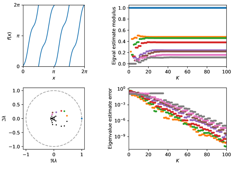
Figure 1: Top left: graph of the circle map $f(x)=4x-0.4\sin 6x+0.08\cos 3x\mod 2\pi$. Bottom left: Ruelle-Pollicott resonances (i.e. Perron-Frobenius operator eigenvalues) of $f$ with certain eigenvalues marked in colour. Top right: modulus of EDMD eigenvalues obtained with $\mu$ the physical measure of $f$, with colours corresponding to eigenvalues in the bottom left. Bottom right: exponential convergence with respect to dictionary size of the errors between EDMD eigenvalues and Ruelle-Pollicott responances, with corresponding colours. Ruelle-Pollicott resonances estimated using a Fourier transfer operator discretisation [34].

1.3 Main result on EDMD

The EDMD algorithm makes a best approximation of the Koopman operator $\mathcal{K}$ in $L^{2}(\mu_{N})$ within the span of the observable dictionary $\Psi=\{\psi_{k}\}_{|k|\leq K}$. This is done with respect to the inner product of $L^{2}(\mu_{N})$, where $\mu_{N}$ is the empirical measure of the data points $\{x_{n}\}_{n=1,\ldots,N}$. This least-squares approximation of $\mathcal{K}$ can be computed in the $\Psi$ basis as the Koopman matrix

$$(\Psi_{(0)}^{*}\Psi_{(0)})^{-1}\Psi_{(0)}^{*}\Psi_{(1)}$$

where $(\Psi_{(0)})_{nk}=\psi_{k}(x_{n})$ and $(\Psi_{(1)})_{nk}=\mathcal{K}\psi_{k}(x_{n})=\psi_{k}(f(x_{n}))$. The key benefit of EDMD over other algorithms is that these matrices can be filled directly from observations of the system.

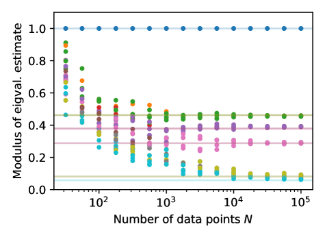
Figure 3: Convergence of the EDMD operator spectrum for fixed approximation size $K=8$ as the number of data points goes to infinity. In pale lines, the corresponding spectrum.

As the number of points $N$ goes to infinity, this converges to the (still finite-dimensional) continuum limit operator $\mathcal{K}_{K}$, which is the least-squares best approximation in $L^{2}(\mu)$ of $\mathcal{K}$ within the dictionary of observables $\operatorname{span}\{\psi_{k}\}$ [25]. As a result, the Koopman matrix’s spectral data also converge to those of the continuum limit operator $\mathcal{K}_{K}$ (see Figure 3).

The main result of this paper is as follows. Let $\lambda_{j,K}$ be the eigenvalues of the EDMD estimate of the Koopman operator $\mathcal{K}_{K}$ obtained using the function dictionary

$$\{e^{-i(K-1)x},e^{-i(K-2)x},\ldots,e^{-ix},1,e^{ix},\ldots,e^{i(K-1)x}\},$$ (2)

in the limit of infinite data points. Each of these eigenvalues, which will be simple for $K$ large enough if the corresponding $\lambda_{j}$ is simple, have left and right eigenvectors $a_{j,K},b_{j,K}\in C^{0}$, which we can consider in the observable basis. Let $\beta_{j,K}(w)=\int b_{j,K}(x)w(x)\mathrm{d}\mu(x)$.

Theorem 1.2.

Suppose $f$ is analytic and $\mu$ has analytic density. Then for some $c>0$ $d_{\rm Haus}(\sigma(\mathcal{K}_{K}),\{\lambda_{j}:j\in\mathbb{N}\})=\mathcal{O}(e^{-c\sqrt{K}})$ as $K\to\infty$.

Furthermore, if $\lambda_{j}$ has multiplicity $1$ (see Theorem 2.1 for a more general result), then there exist constants $h,\zeta>0$ depending on $f,\mu$ such that for $t\in[0,\zeta]$,

$$|\lambda_{j,K}-\lambda_{j}|,\|a_{j,K}-a_{j}\|_{\mathcal{H}^{2}_{t}},\|b_{j,K}-b_{j}\|_{\mathcal{H}^{2}_{-t}}=\mathcal{O}(e^{-htK}).$$

An illustration of this theorem is given in Figure 1, with eigenvalue estimates converging exponentially with the dictionary size $K$ as predicted: note that the leading constants generally increase as the modulus of the eigenvalue decreases.

The consequence of Theorem 1.2 is that, in this setting, EDMD gives very accurate estimates about the system’s rates of mixing, encoded through the Ruelle-Pollicott resonances. It also means that the so-called DMD modes (or left Koopman modes) $a_{j,K}$ and (right) Koopman modes” $\beta_{j,K}$ obtained respectively as left and right eigenvectors of the Koopman operator approximation closely approximate certain limiting objects that give information about the long-term dynamical properties of the system. The limiting function $a_{j}$ and functional $\beta_{j}$ encode structures that persist under the dynamics, including almost-invariant sets [19, 17]. Notwithstanding that the maps we consider are extremely structurally simple, this may go some way to explaining the success of DMD with small dictionaries.

It is worth noting however that the left Koopman modes $b_{j,K}$ converge in the space of hyper-distributions $\mathcal{H}^{2}_{-t}$ to the functional $\beta_{j}$, which does not make sense as a function in the proper sense of the word, but rather as something you can integrate sufficiently differentiable functions against. In particular, the $b_{j,K}$ do not converge pointwise or in $L^{2}$. This situation is illustrated in Figure 2: for low orders $K$ the right Koopman modes $b_{j,K}$ do in fact appear like “nice” enough functions that delimit almost-invariant sets, but as the resolution of the approximation (i.e. $K$) increases they become increasingly irregular: the consistency of the envelope of the functions in Figure 2 nevertheless suggests that they under some smoothing they may consistently return functions delimiting almost-invariant sets.

The overarching strategy to prove Theorem 1.2 parallels that sketched in [31], i.e. we study by duality a transfer operator acting on Hilbert spaces $\{\mathcal{H}^{2}_{t}\}_{t\in(0,\zeta]}$ of analytic functions, and consider the effect of the least squares projection onto the finite observable space (2) in these Hilbert spaces: Theorem 1.1 allows us to bound the error of $\mathcal{P}_{K}$ from our Hardy spaces $\mathcal{H}^{2}_{t}\to\mathcal{H}^{2}_{s}$ as $\mathcal{O}(e^{-(t-s)})$ for small enough $t,s$ for analytic measure densities $h$, which is enough to obtain this result.

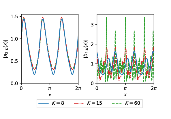
Figure 2: For the circle map given in Figure 1, the absolute value of the left (left plot) and right (right plot) eigenmodes of the Koopman operator approximation $\mathcal{K}_{K}$ corresponding to the second-largest eigenvalue. The different modes of convergence (respectively in a very strong norm, and weakly, as a hyperdistribution) are shown.

We have been careful to make our results as tight as possible, but there are places where they could be meaningfully improved. In particular, in proving the least-squares approximation result, we bounded the operator norms of certain operators in Proposition 4.9 via the trace norm, which would scale poorly into higher dimensions, and even in one dimension requires $\mu$ to be at least half an order more differentiable than the functions it is approximating.

This would make it difficult to apply our methods to study EDMD with respect to less regular densities—which naturally occur as physical meaures of chaotic systems and therefore as the sampling measure for time series. A salutary example is for the logistic map $f(x)=ax(1-x)$, which is chaotic for a positive measure set of parameters $a\in[3.5,4]$, and which models the non-hyperbolic dynamics which are standard in fluid flow. Chaotic logistic maps typically have a physical measure whose density contains inverse square root singularities, and therefore lacks the level of differentiability required for our results [29]. Further work, perhaps building on OPUC theory in [21], might show a path through, and establish how well DMD works with the kinds of irregular sampling measures typical of most chaotic dynamics.

In this work we have of course put aside an important, indeed limiting, component: the effect of the data discretisation. We know that this converges weakly as the empirical measure of the data $\{x_{n}\}$ converges weakly to the limiting measure $\mathrm{d}\mu(x)$ [25]: there are many results showing this, including for time series data $x_{n+1}=f(x_{n})$, where we know the rate of convergence is the central limit theorem rate $\mathcal{O}(N^{-1/2})$ [11]. This is borne out in simulations: see Figure 2. Nevertheless, this rate of convergence may also depend on the size of the dictionary (i.e. on $K$), a key direction for future work.

1.4 Paper plan

This paper is structured as follows. In Section 2 we make a precise statement of our assumptions on the system and the corresponding theorems. In Section 3 we relate the $L^{2}(\mu)$-orthogonal trigonometric polynomials to a Cholesky decomposition of multiplication by $\mu$ in a Fourier basis, and in Section 4 quantitatively characterise this decomposition to prove Theorem 1.1. Finally in Section 5 we combine this result with transfer operator results to obtain our theorems on EDMD.

2 Detailed setup and theorems

In this section we will state the precise condition on the map $f$ and sampling density $\mu$ that we require, and state our Koopman operator approximation theorems in generality.

We will make base our function spaces on extensions of the standard $L^{p}$ spaces on the torus $\mathbb{T}=\mathbb{R}/2\pi\mathbb{Z}$. Recall the $L^{p}$ norms are defined as

$$\|\varphi\|_{L^{p}(\mathbb{T})}=\begin{cases}\left(\int_{0}^{2\pi}|\varphi(x)|^{p}\,\mathrm{d}x\right)^{1/p},&p\in[1,\infty)\\ \operatorname{ess-sup}_{x\in\mathbb{T}}|\varphi(x)|,&p=\infty.\end{cases}$$

However, we will need to construct stronger function spaces to obtain effective results. In particular, we will look at on certain open complex strips in phase space around $\mathbb{T}$, which we will parametrise by their half-thickness $\zeta$:

$$\mathbb{T}_{\zeta}:=\{z\in\mathbb{C}/2\pi\mathbb{Z}:|\Im z|<\zeta\}$$

On these sets we will define so-called Hardy spaces $\mathcal{H}^{p}_{\zeta}$ for $\zeta>0$: the space $\mathcal{H}^{p}_{\zeta}$ is the set of holomorphic functions $\varphi:\mathbb{T}_{\zeta}\to\mathbb{C}$ such that

$$\|\varphi\|_{\mathcal{H}^{p}_{\zeta}}:=\begin{cases}\sup_{\beta\in[0,\zeta)}\left(\frac{1}{4\pi}\int_{\mathbb{T}}|\varphi(\theta+i\beta)|^{p}+|\varphi(\theta-i\beta)|^{p}\,\mathrm{d}\theta\right)^{1/p},&p\in[1,\infty)\\ \sup_{z\in\mathbb{T}_{\zeta}}|\varphi|,&p=\infty\end{cases}$$

is finite (in which the supremum is attained in the limit as $\beta\to\zeta$, and $\varphi$ is continuous onto $\partial\mathbb{T}_{\zeta}$ almost everywhere). The $L^{p}(\mathbb{T})$ norms emerge as a limiting case as $\zeta\to 0$. (For concision, we will define $\|\cdot\|_{\mathcal{H}^{p}_{0}}=\|\cdot\|_{L^{p}(\mathbb{T})}$).

The spaces $\mathcal{H}^{2}_{\zeta}$ are Hilbert spaces, and we can characterise these norms in Fourier space. Let $\mathcal{F}:L^{2}(\mathbb{T})\to\ell_{2}(\mathbb{Z})$ be the Fourier series operator:

$$(\mathcal{F}\varphi)(k)=\frac{1}{2\pi}\int_{\mathbb{T}}e^{-ikx}\varphi(x)\,\mathrm{d}x$$

and for $\sigma$ a Beurling weight let us define the Hilbert spaces $W^{\sigma}(\mathbb{T})=\mathcal{F}^{-1}[\sigma\ell^{2}(\mathbb{Z})]$ with

$$\|\varphi\|_{W^{\sigma}}=\|\sigma\mathcal{F}\varphi\|_{\ell^{2}(\mathbb{Z})}.$$

It is a classic result that the standard $L^{2}(\mathbb{T})$ is such a space with $\sigma(n)\equiv 1$; Sobolev spaces $H^{r}$ are isometric to those with $\sigma(n)=(1+n^{2})^{r/2}$. Similarly, if we define the Beurling weight

$$\sigma_{\zeta}(k):=\sqrt{\cosh 2k\zeta},$$

then we can write our Hardy space $\mathcal{H}^{2}_{\zeta}(\mathbb{T})=W^{\sigma_{\zeta}}$.

We can also define adjoints of these spaces: for a Beurling weight $\sigma$ let $W^{\sigma^{-1}}$ be the completion of $L^{2}(\mathbb{T})$ with respect to the following norm:

$$\|\varphi\|_{W^{\sigma^{-1}}}=\sup_{\|\psi\|_{W^{\sigma}}=1}\frac{1}{2\pi}\int_{\mathbb{T}}\varphi\psi\,\mathrm{d}\theta.$$

This Hilbert space $W^{\sigma^{-1}}$ is therefore isometric to $\sigma^{-1}\ell^{2}$ under the Fourier series operator $\mathcal{F}$. We can of course therefore define $\mathcal{H}^{2}_{-\zeta}=W^{\sigma_{\zeta}^{-1}}$ as the dual of $\mathcal{H}^{2}_{\zeta}$.

We will use the notation $\mathcal{A}^{\dagger}$ to stand for the adjoint operator of $\mathcal{A}$ in $L^{2}(\mathbb{T},\mathrm{\operatorname{Leb}}/2\pi)$, and extend this to functions: $\phi^{\dagger}\psi:=\int_{\mathbb{T}}\bar{\phi}\psi\,\mathrm{d}x$.

Our basic assumptions will be that map $f$ is uniformly expanding and real-analytic and the sampling measure $\mu$ has real-analytic density $h(x)$ with respect to Lebesgue. Note that if $\mu$ is the absolutely continuous invariant measure of $f$, then the first part implies the second.

To better understand rates of convergence, we will make the following quantitative assumptions on $f$ for some $\zeta>0$:

• The lift of $f$ onto $\mathbb{R}$ has an inverse $v:\mathbb{R}\to\mathbb{R}$ that extends analytically to $\mathbb{R}_{\zeta}:=\mathbb{R}+i[-\zeta,\zeta]$.

• For $z\in\mathbb{R}_{\zeta}$, $|v^{\prime}(z)|\leq\gamma^{-1}$ for some $\gamma<1$.

• $\|\log(v^{\prime})\|_{C^{\alpha}(\mathbb{T}_{\zeta})}\leq D$ for some constants $\alpha>0$ and $D\leq\tfrac{\pi}{3}\zeta^{-\alpha}$.

The last bound can always be achieved by making $\zeta$ smaller.

When studying the convergence of extended dynamical mode decomposition, we will also make the following quantitative assumptions on $h$:

• $h$ extends analytically to $\mathbb{T}_{\zeta}$.

• For $z\in\mathbb{T}_{\zeta}$, $M^{-1}\leq|h(z)|\leq M$ for some constant $M$.

• $\|\sigma\mathcal{F}[(\log h)^{\prime}]\|_{\ell^{q}}\leq A$ for some constants $A$ and $q<\infty$. (Note this occurs if $(\log h)^{\prime}\in L^{p}(\partial\mathbb{T}_{\zeta})$ where $1/p+1/q=1$.)

The key to our results on spectral convergence is the following strong operator convergence result:

Theorem 2.1.

For all $t\in(0,\zeta]$ the Koopman operator $\mathcal{K}:\mathcal{H}^{2}_{-t}\circlearrowleft$ is compact, the sequence of operators $\{\mathcal{K}_{K}:\mathcal{H}^{2}_{-t}\circlearrowleft\}_{K\in\mathbb{N}}$ is collectively compact, and there exists a constant $C$ depending only on $M,A,D,\zeta$ such that

$$\|\mathcal{K}_{K}-\mathcal{K}\|_{\mathcal{H}^{2}_{-t}}\leq Ce^{-(1-\gamma^{-1})tK}.$$

This allows us to estimate all the eigenmodes and Ruelle-Pollicott resonances of the system in (1):

Corollary 2.2.

For all $\mathcal{K}$’s eigenvalues $\lambda$ of multiplicity $m$, the error in the $\mathcal{K}_{K}$ estimate as $K\to\infty$ is $\mathcal{O}(e^{-(1-\gamma^{-1})\zeta K/m})$ for the eigenvalues, and $\mathcal{O}(e^{-(1-\gamma^{-1})tK})$ in $H^{2}_{-t}$ (resp. $H^{2}_{\gamma^{-1}t}$) for the right (resp. left) generalised eigenspaces.

3 Cholesky factorisation

To understand the $\mu$-orthogonal projection onto our dictionary of complex exponential basis functions $\{e_{k}\}_{|k|\leq K}$, it will be natural to understand the transformation between the complete, infinite basis $\{e_{k}\}_{k\in\mathbb{Z}}$ and an orthogonal polynomial basis of $L^{2}(\mu)$ (in which the $L^{2}(\mu)$ projection is therefore diagonal). In the correct ordering it is known that the basis change matrices are triangular and asymptotically banded [30]: we will prove some quantitative results on the rate of convergence to bandedness as the order of the polynomial grows.

Recall that the complex exponential family on $\mathbb{C}/2\pi\mathbb{Z}\supset\mathbb{T}$

$$e_{k}(z):=e^{ikz},\,k\in\mathbb{Z},$$

is a basis both of $L^{2}(\mathbb{T})$ and our Beurling-weighted spaces $W^{\sigma}$. For the purposes of this section, let us order the basis’ index set $\mathbb{Z}$ as

$$0,-1,1,-2,2,-3,3,\ldots$$

and group the basis elements into “blocks” $\{e_{0}\},\{e_{-1},e_{1}\},\{e_{-2},e_{2}\},\ldots$.

For any positive probability density $h:\mathbb{T}\to\mathbb{R}_{+}$, define the Fourier space multiplication operator $\mathcal{M}:L^{2}(\mathbb{T})\to L^{2}(\mathbb{T})$:

$$\mathcal{M}\varphi=h\varphi.$$ (3)

The operator $\mathcal{M}$ is positive-definite and Hermitian in $L^{2}(\mathbb{T})$. (In fact, in Fourier space it is near-block-Toeplitz with respect to our basis order.) It turns out we can make a Cholesky decomposition of $\mathcal{M}$ that is very nicely, uniformly bounded in our Hardy or Beurling-weighted Hilbert spaces, under our analyticity assumptions on $h$:

Proposition 3.1.

Supposing only that $\log h\in L^{\infty}$, there exists a unique lower triangular operator $\mathcal{V}$ acting on $L^{2}(\mathbb{T})$ such that

$$\mathcal{M}=\mathcal{V}\mathcal{V}^{\dagger}.$$

Furthermore, $\mathcal{V}$ is invertible. If we let $\mathcal{V}^{-1}=:\mathcal{U}^{\dagger}$, the operator $\mathcal{U}$ is upper-triangular with

$$\mathcal{M}^{-1}=\mathcal{U}^{\dagger}\mathcal{U}.$$

Proof of Proposition 3.1.

Let us consider $\mathcal{M}$ as an infinite matrix acting on the basis

$$1,\sin z,\cos z,\sin 2z,\cos 2z,\ldots$$

The matrix of $\mathcal{M}$ is real and positive-definite, bounded on $L^{2}(\mathbb{T})$. By [12, Lemma 3.1], there exists a unique lower-triangular operator $\mathcal{V}_{\mathbb{R}}$ such that $\mathcal{M}=\mathcal{V}_{\mathbb{R}}\mathcal{V}_{\mathbb{R}}^{\dagger}$. Now, for any function $\varphi\in L^{2}(\mathbb{T})$,

$$\varphi^{\dagger}\mathcal{M}\varphi=\varphi^{\dagger}\mathcal{V}_{\mathbb{R}}\mathcal{V}_{\mathbb{R}}^{\dagger}\varphi=\|\mathcal{V}_{\mathbb{R}}^{\dagger}\varphi\|_{L^{2}}^{2}$$ (4)

so since $\mathcal{M}\varphi=h\varphi$,

$$M^{-1}\|\varphi\|_{L^{2}}^{2}\leq\|\mathcal{V}_{\mathbb{R}}^{\dagger}\varphi\|_{L^{2}}^{2}\leq M\|\varphi\|_{L^{2}}.$$ (5)

Since, $\mathcal{V}^{\dagger}_{\mathbb{R}}$ is bounded in $L^{2}(\mathbb{T})$, so too is its adjoint $\mathcal{V}_{\mathbb{R}}$ and its inverse $\mathcal{U}_{\mathbb{R}}$. Now, $\mathcal{V}^{\dagger}_{\mathbb{R}}$ is block-lower triangular in the complex exponential basis $e_{k}$, the blocks consisting of $\{e_{k},e_{-k}\}$. We can perform a $LQ$ decomposition on each block to obtain a block-diagonal unitary matrix $\mathcal{Q}$ such that $\mathcal{V}=\mathcal{V}_{\mathbb{R}}\mathcal{Q}$ is lower-triangular in the complex exponential basis, and $\mathcal{U}=\mathcal{Q}\mathcal{U}_{\mathbb{R}}$ is upper-triangular in this basis with $\mathcal{V}\mathcal{V}^{\dagger}=\mathcal{M}$ and $\mathcal{U}^{\dagger}\mathcal{U}=\mathcal{M}^{-1}$. ∎

Now, define the functions

$$p_{k}=\mathcal{U}e_{k}.$$

From the proposition above, it turns out that these are a complete family of (complex) trigonometric polynomials orthonormal with respect to $h$:

Proposition 3.2.

The $p_{k}$ are each trigonometric polynomials of order exactly $|k|$, and form a complete orthonormal basis in $L^{2}(\mu)$.

Proof.

Integrating two polynomials against each other,

$$\int_{\mathbb{T}}\overline{p_{j}}p_{k}\,\mathrm{d}\mu =(\mathcal{U}e_{j})^{\dagger}h\mathcal{U}e_{k}$$

$$=e_{j}^{\dagger}\mathcal{U}^{\dagger}((\mathcal{U}^{\dagger})^{-1}\mathcal{U}^{-1})\mathcal{U}e_{k}$$

$$=e_{j}^{\dagger}e_{k}=\delta_{jk},$$

as required for orthonormality. Because $\mathcal{U}$ is upper-triangular in the complex exponential basis with non-zero diagonals, $\mathcal{U}e_{k}$ is a combination of complex exponentials of order no greater than $|k|$, so $p_{k}$ is a trigonometric polynomial of the right order.

On the other hand, the complex exponentials $\{e_{k}\}_{k\in\mathbb{Z}}$ form a complete basis of $L^{2}(\mathbb{T},\mathrm{\operatorname{Leb}})$ and hence of $L^{2}(\mathbb{T},\mu)$, as the spaces are equivalent. But the $p_{k}$ are preimages of $e_{k}$ under $\mathcal{U}^{-1}:L^{2}(\mathbb{T},\mu)\circlearrowleft$, so $\{p_{k}\}_{k\in\mathbb{Z}}$ must therefore, like $\{e_{k}\}_{k\in\mathbb{Z}}$, be a complete basis of $L^{2}$. ∎

The $p_{k}$ as described here are complex, but they can be transformed via a unitary map into a real orthonormal family (see the proof of Proposition 3.1): we have only chosen a complex exponential basis for the simplicity of the following presentation.

The corollary of Proposition 3.1 is that $L^{2}(\mu)$-orthogonal projection is conjugate to the usual $L^{2}(\operatorname{Leb})$ projection (i.e. the Dirichlet kernel, whose properties are very well known):

Proposition 3.3.

Let $\mathcal{P}_{K}:L^{2}(\mu)\circlearrowleft$ be the orthogonal projection onto trigonometric polynomials of order $<K$. Then

$$\mathcal{P}_{K}=\mathcal{U}^{-1}\mathcal{D}_{K}\mathcal{U}=\mathcal{V}^{\dagger}\mathcal{D}_{K}\mathcal{U}$$

where $\mathcal{D}_{K}=\mathcal{F}^{-1}\mathbb{1}_{(-K+1,\ldots,K-1)}\mathcal{F}$ is convolution by the Dirichlet kernel.

Proof.

Since $\{e_{k}\}_{k\in\mathbb{Z}}$ is a complete basis of $L^{2}(\mathbb{T})$, and the $p_{k}$ are obtained from the $e_{k}$ by the transformation $\mathcal{U}$, which from Proposition 3.1 we know is invertible on $L^{2}(\mathbb{T})$, our polynomials $\{p_{k}\}_{k\in\mathbb{Z}}$ form a complete basis of $L^{2}(\operatorname{Leb})=L^{2}(\mu)$, setting $\sigma\equiv 1$. (Indeed, applying Theorem 4.1 below instead of Proposition 3.1, we can say that this is true in the Beurling weighted spaces $W^{\sigma}$.)

The action of $\mathcal{P}_{K}$ on our basis is $\mathcal{P}_{K}p_{k}=\mathbb{1}_{|k|<K}p_{k}$. Using from Proposition 3.2 that $p_{k}=\mathcal{U}e_{k}$, we can conjugate by $\mathcal{U}$ to obtain

$$\mathcal{U}^{-1}\mathcal{P}_{K}\mathcal{U}e_{k}=\mathbb{1}_{|k|\leq K}e_{k}.$$

Since the action of $\mathcal{U}^{-1}\mathcal{P}_{K}\mathcal{U}$ is precisely the action of $\mathcal{D}_{K}$, and $\mathcal{U}^{-1}=\mathcal{V}^{\dagger}$, we obtain that $\mathcal{P}_{K}=\mathcal{U}^{-1}\mathcal{D}_{K}\mathcal{U}=\mathcal{V}^{\dagger}\mathcal{D}_{K}\mathcal{U}$ as required. ∎

Thus motivated to study Cholesky decompositions of multiplication operators, we embark on proving that such things exist and their constituents are bounded in $W^{\sigma}$.

4 Proof of orthogonal polynomial results

We would like to understand our orthogonal projection $\mathcal{P}_{K}$ in the Beurling weighted spaces $W^{\sigma}$. Proposition 3.3 suggests that we should therefore study the norm of triangular operators $\mathcal{U},\mathcal{V}$ in these weighted spaces. The following result, which we will spend this section proving, shows that these operators are uniformly bounded:

Theorem 4.1.

Under the assumptions on $\mu$ in Theorem 1.1, there exists a constant $C_{\triangle}$ increasing in $q,M,A$ such that

$$\|\mathcal{U}\|_{W^{\sigma}},\|\mathcal{V}\|_{W^{\sigma}},\|\mathcal{U}^{\dagger}\|_{W^{\sigma}},\|\mathcal{V}^{\dagger}\|_{W^{\sigma}}\leq C_{\triangle}.$$

Our goal is to show that these operators $\mathcal{U},\mathcal{V}$ obtained by Cholesky decomposition of a multiplication operator $\mathcal{M}$ approximate multiplication operators themselves, at least when acting on functions of high frequency.

To this end, let $\theta^{+},\theta^{-}$ be real-analytic functions $\mathbb{T}\to\mathbb{C}$ such that $\theta^{-}(\bar{z})=\overline{\theta^{+}(z)}$, $\theta^{+}\theta^{-}=1/h$ and $\theta^{+}$ is holomorphic in the upper half-plane. We can specify them explicitly:

$$(\mathcal{F}\log\theta^{+})(k)=\left(\tfrac{1}{2}\delta_{0k}+\mathbb{1}(k>0)\right)\mathcal{F}(-\log h)(k).$$ (6)

and similarly for $\theta^{-}$ with $\mathbb{1}(k<0)$ replacing $\mathbb{1}(k>0)$. In the language of orthogonal polynomials on the unit circle (where one studies the variable $z=e^{ix}$), the function $\theta^{+}(\log z)$ is known as the Szegő function of $\mathrm{d}\mu(\log z)$ [30]. We will also notate their reciprocals $\eta^{\pm}=1/\theta^{\pm}$. The following result states some of the basic properties of $\theta^{\pm},\eta^{\pm}$ (c.f. [30, Theorem 2.4.1]).

Proposition 4.2.

Under our assumptions on $h$:

1. For all $x\in\mathbb{T}$ we have

   $$|\theta^{+}(x)|=|\theta^{-}(x)|=\sqrt{h(x)}.$$

2. Considering functions as multiplication operators,

   $$\|\theta^{\pm}\|_{W^{\sigma}\to W^{\sigma}},\|\eta^{\pm}\|_{W^{\sigma}\to W^{\sigma}}\leq M^{1/2}e^{qA}.$$

3. If $\hat{\theta}^{+}_{l}$ are the Fourier coefficients of $\theta^{+}$, then

   $$\sum_{l=0}^{\infty}l\sigma(l)^{2}|\hat{\theta}^{+}_{l}|^{2}\leq qA^{2}Me^{2qA}.$$

We will briefly find it useful to notate some $\l^{p}$-type norms associated with the Beurling weights. For $q\in[1,\infty]$ let $\|\varphi\|_{\sigma;q}=\|\sigma\mathcal{F}\varphi\|_{\ell^{q}}$.

Lemma 4.3.

Suppose $\sigma$ is a Beurling weight. Then for any $q\in[1,\infty]$,

$$\|\varphi\psi\|_{\sigma;q}\leq\|\varphi\|_{\sigma;q}\|\psi\|_{\sigma;1}$$

whenever $\|\varphi\|_{\sigma;r},\|\psi\|_{\sigma;1}<\infty$.

Proof.

All we need to prove is that $\|\sigma(\hat{\varphi}\ast\hat{\psi})\|_{\ell^{q}}\leq\|\sigma\hat{\varphi}\|_{\ell^{q}}\|\sigma\hat{\psi}\|_{\ell^{q}}.$

By the definition of the Beurling weight, $\sigma(k)\leq\sigma(|j|+|k-j|)\leq\sigma(j)\sigma(k-j)$, so

$$|\sigma(k)(\hat{\varphi}\ast\hat{\psi})(k)| =\sum_{j\in\mathbb{Z}}\sigma(k)|\hat{\varphi}(j)||\hat{\psi}(k-j)|$$

$$\leq\sum_{j\in\mathbb{Z}}|\sigma(j)\hat{\varphi}(j)||\sigma(k-j)\hat{\psi}(k-j)|$$

$$\leq(|\sigma\hat{\varphi}|\ast|\sigma\hat{\psi}|)(k)$$

As a result,

$$\|\sigma(\hat{\varphi}\ast\hat{\psi})\|_{\ell^{q}}\leq\||\sigma\hat{\varphi}|\ast|\sigma\hat{\psi}|\|_{\ell^{q}}\leq\|\sigma\hat{\varphi}\|_{\ell^{q}}\|\sigma\hat{\psi}\|_{\ell^{1}}$$

as required. ∎

Proof of Proposition 4.2.

We only need to prove the results for $\theta^{+}$, as $\log\theta^{+}(\bar{z})=\overline{\log\theta^{-}(z)}$.

The first part directly uses this fact: $|\theta^{+}(x)|^{2}=\theta^{-}(x)\theta^{+}(x)=h(x)^{-1}$.

To prove the second part, we separate $k=0$ and apply Hölder’s inequality to get

$$\|\log h\|_{\sigma;1}\leq\sigma(0)\left|\int\log h\,\mathrm{d}x\right|+\|\sigma(k)k\mathcal{F}[\log h](k)\|_{\ell^{q}}\|\mathbb{1}_{k\neq 0}k^{-1}\|_{\ell^{p}}$$

where $1/p+1/q=1$. Noting that by submultiplicativity $\sigma(0)\leq 1$, this gives us

$$\|\log h\|_{\sigma;1}\leq\log M+\|(\log h)^{\prime}\|_{\sigma;q}(2\zeta(p))^{1/p}\leq\log M+A(2q)^{1/p}\leq\log M+2qA.$$

Noting that $\log h$ is real on $\mathbb{T}$, (6) gives us that

$$\|\log\theta^{+}\|_{\sigma;1}=\tfrac{1}{2}\|\log h\|_{\sigma;1}=\log M^{1/2}+qA.$$

Now, $\theta^{+}$ and $\eta^{+}=\tfrac{1}{\theta^{+}}$ are respectively the $t=1,-1$ solutions of

$$\frac{\partial}{\partial t}\mathcal{E}_{t}(x)=\log\theta^{+}\,\mathcal{E}_{t}(x),\,\mathcal{E}_{0}(x)=1$$

so Gronwall’s Lemma combined with Lemma 4.3 gives

$$\|\theta^{+}\|_{\sigma;1},\|\eta^{+}\|_{\sigma;1}\leq e^{\|\log\theta^{+}\|_{\sigma;1}}\|1\|_{\sigma;1}\leq e^{qA}M^{1/2}.$$

The bounds on $\theta^{+},\eta^{+}$ considered as multipliers on $W^{\sigma}$ (which has the $\|\cdot\|_{\sigma;2}$ norm) follows from Lemma 4.3.

For the third part we proceed in the same vein as the second part. From (6) we have $\mathcal{F}(\log\theta_{+})^{\prime}=\mathbb{1}(k>0)\mathcal{F}(-\log h)(k)$, so $\|\sigma\mathcal{F}[(\log\theta_{+})^{\prime}]\|_{\ell^{q}}\leq A$. Then,

$$\|(\theta^{+})^{\prime}\|_{\sigma;q}=\|(\log\theta^{+})^{\prime}\|_{\sigma;q}\|\theta^{+}\|_{\sigma;1}\leq AM^{1/2}e^{qA}.$$

Applying Hölder’s inequality gives that

$$\|k^{1/2}\sigma\mathcal{F}[\theta^{+}]\|_{\ell_{2}}^{2} =\|(\mathbb{1}(k\neq 0)k^{-1/2})\sigma\mathcal{F}[(\theta^{+})^{\prime}]\|_{\ell^{2}}^{2}$$

$$\leq\|\mathbb{1}(k\neq 0)k^{-1}\|_{\ell^{q/(q-2)}}\|(\theta^{+})^{\prime}\|_{\sigma;q}^{2}$$

$$\leq qA^{2}Me^{2qA},$$

which is what needed to be proven. ∎

With these properties in hand we can now characterise the asymptotically banded structure of the Cholesky decomposition.

Define the projections

$$\mathcal{P}^{+} =\mathcal{F}^{-1}\mathbb{1}_{\mathbb{Z}^{+}}\mathcal{F}$$

$$\mathcal{P}^{\circ} =\mathcal{F}^{-1}\mathbb{1}_{\{0\}}\mathcal{F}=e_{0}e_{0}^{\dagger}$$

$$\mathcal{P}^{-} =\mathcal{F}^{-1}\mathbb{1}_{\mathbb{Z}^{-}}\mathcal{F}.$$

The limiting Cholesky factors, which describe the action of $\mathcal{U},\mathcal{V}$ on $e_{k}$ with $|k|$ large, are

$${\bar{\mathcal{U}}}={\bar{c}}\mathcal{P}^{\circ}+\mathcal{P}^{+}\theta^{-}+\mathcal{P}^{-}\theta^{+}.$$

$${\bar{\mathcal{V}}}={\bar{c}}^{-1}\mathcal{P}^{\circ}+\eta^{+}\mathcal{P}^{+}+\eta^{-}\mathcal{P}^{-}$$

where ${\bar{c}}$ is an arbitrary constant: we set ${\bar{c}}=\sqrt{\tfrac{1}{2\pi}\int h^{-1}\,\mathrm{d}x}$.

These obey the same relation as their equivalents $\mathcal{V},\mathcal{U}$ do:

Lemma 4.4.

${\bar{\mathcal{V}}}^{-1}={\bar{\mathcal{U}}}^{\dagger}$.

Proof.

If $\psi^{+}$ contains only non-negative Fourier modes, then $\psi^{+}\mathcal{P}^{+}=\mathcal{P}^{+}\psi^{+}\mathcal{P}^{+}$, with the corresponding result for functions with non-positive modes.

We have that ${\bar{\mathcal{U}}}^{\dagger}={\bar{c}}\mathcal{P}^{\circ}+\theta^{+}\mathcal{P}^{+}+\theta^{-}\mathcal{P}^{-}$, and the result follows by expanding out ${\bar{\mathcal{U}}}^{\dagger}{\bar{\mathcal{V}}}$ and ${\bar{\mathcal{V}}}{\bar{\mathcal{U}}}^{\dagger}$. ∎

These operators are uniformly bounded:

Lemma 4.5.

For all $t\in[0,\zeta]$,

$$\|{\bar{\mathcal{U}}}\|_{W^{\sigma}},\|{\bar{\mathcal{U}}}^{\dagger}\|_{W^{\sigma}},\|{\bar{\mathcal{V}}}\|_{W^{\sigma}},\|{\bar{\mathcal{V}}}^{\dagger}\|_{W^{\sigma}}\leq(1+2e^{qA})M^{1/2}.$$

Proof.

Since the projections $\mathcal{P}^{+},\mathcal{P}^{-},\mathcal{P}^{\circ}$ have norm $1$ in $W^{\sigma}$,

$$\|{\bar{\mathcal{U}}}\|_{W^{\sigma}}\leq{\bar{c}}+\|\theta^{+}\|_{W^{\sigma}\to W^{\sigma}}+\|\theta^{-}\|_{W^{\sigma}\to W^{\sigma}}\leq(1+2e^{qA})M^{1/2}.$$

The same argument goes for the other operators. ∎

Lemma 4.6.

If $\mathcal{P}^{+}w=0$, then $\mathcal{P}^{+}w-w\mathcal{P}^{+}=(\mathcal{P}^{-}+\mathcal{P}^{\circ})w\mathcal{P}^{+}$. The same statement holds swapping $\mathcal{P}^{+}$ and $\mathcal{P}^{-}$.

Proof.

For $k\leq 0$ the operator $\mathcal{P}^{+}e^{-ik\cdot}\mathcal{P}^{+}$ reduces to $\mathcal{P}^{+}e^{ik\cdot}$. Since we have that $w(z)=\sum_{k=0}^{\infty}\hat{w}_{-k}e^{-ikz}$ so $\mathcal{P}^{+}w\mathcal{P}^{+}=\mathcal{P}^{+}w$. Then,

$$\mathcal{P}^{+}w-w\mathcal{P}^{+}=(I-\mathcal{P}^{+})w\mathcal{P}^{+}=\mathcal{P}^{\circ}w\mathcal{P}^{+}+\mathcal{P}^{-}w\mathcal{P}^{+}.$$

∎

We will want to show that in some sense ${\bar{\mathcal{V}}}$ is a good approximation of $\mathcal{V}$, the Cholesky factor of $\mathcal{M}$, and similarly ${\bar{\mathcal{U}}}$ is a good approximation of $\mathcal{U}$. We can understand this by attempting to “strip” $\mathcal{M}$ down to the identity, by considering ${\bar{\mathcal{V}}}^{\dagger}\mathcal{M}^{-1}{\bar{\mathcal{V}}}$ and ${\bar{\mathcal{U}}}^{\dagger}\mathcal{M}{\bar{\mathcal{U}}}$. (It is useful to study both at the same time: in Proposition 4.9 we will use one-sided bounds on each one to complete the bounds on the other.)

It will turn out in Proposition 4.9 that all we need to know are the diagonal entries of these operators. In the following two propositions, we will show that these entries converge to those of the identity (c.f. [30, Proposition 2.4.7, Theorem 7.2.1]).

Lemma 4.7.

For all $k\in\mathbb{Z}$,

$$s^{\prime}_{k}=e^{\dagger}_{k}{\bar{\mathcal{V}}}^{\dagger}\mathcal{M}^{-1}{\bar{\mathcal{V}}}e_{k}-1=0.$$

Proof.

We have

$$1+s^{\prime}_{k}=({\bar{\mathcal{V}}}e_{k})^{\dagger}\mathcal{M}^{-1}({\bar{\mathcal{V}}}e_{k}).$$

When $k=0$,

$${\bar{\mathcal{V}}}e_{0}={\bar{c}}^{-1}e_{0}=(e_{0}^{\dagger}h^{-1})^{-1/2}e_{0}$$

so

$$1+s^{\prime}_{0}=(e_{0}^{\dagger}h^{-1})^{-1}e_{0}^{\dagger}h^{-1}e_{0}=1.$$

On the other hand, when $k>0$ (the $k<0$ case follows by the same argument), ${\bar{\mathcal{V}}}e_{k}=\eta^{+}\mathcal{P}^{+}e_{k}=\eta^{+}e_{k}$ so

$$1+s^{\prime}_{k}=e_{k}^{\dagger}\eta_{-}\eta_{-}\eta_{+}\eta^{+}e_{k}=e_{k}^{\dagger}e_{k}=1,$$

as required. ∎

Lemma 4.8.

Let

$$s_{k}=e^{\dagger}_{k}{\bar{\mathcal{U}}}^{\dagger}\mathcal{M}{\bar{\mathcal{U}}}e_{k}-1.$$

Then $s_{k}>-1$ and there exists a constant $C$ increasing in $M,A,q$ such that

$$\sum_{k\in\mathbb{Z}}\sigma(k)^{2}|s_{k}|\leq C.$$ (7)

Proof.

In this case we have

$$1+s_{k}=({\bar{\mathcal{U}}}e_{k})^{\dagger}\mathcal{M}({\bar{\mathcal{U}}}e_{k}),$$

but the situation is more complicated than in Lemma 4.7 because, when compared with the previous proposition, the order of projection and multiplication in the definition of ${\bar{\mathcal{U}}}$ are now reversed compared with ${\bar{\mathcal{V}}}$. We can use Lemma 4.6 to swap them back, but this means we pay the price of a small error, which we now bound.

For $k=0$ we have that

$${\bar{\mathcal{U}}}e_{0}=\mathcal{P}^{+}\theta_{-}e_{0}+\mathcal{P}^{-}\theta_{+}e_{0}+{\bar{c}}\mathcal{P}^{\circ}e_{0}={\bar{c}}e_{0}$$

so

$$s_{0}=1-{\bar{c}}^{2}e_{0}^{\dagger}he_{0}=1-\frac{1}{2\pi}\int_{T}h^{-1}\,\mathrm{d}x\,\frac{1}{2\pi}\int_{\mathbb{T}}h\,\mathrm{d}x$$

from which one may extract that $|s_{0}|\leq(M-1)^{2}$.

For $k>0$ we have that

$${\bar{\mathcal{U}}}e_{k}=\mathcal{P}^{+}\theta_{-}e_{k}+\mathcal{P}^{-}\theta_{+}e_{k}+{\bar{c}}\mathcal{P}^{\circ}e_{k}=\mathcal{P}^{+}\theta_{-}e_{k},$$

and since $\mathcal{M}=\eta^{+}\eta^{-}=\overline{\eta^{-}}\eta^{-}$,

$$({\bar{\mathcal{U}}}e_{k})^{\dagger}\mathcal{M}({\bar{\mathcal{U}}}e_{k}) =(\eta^{-}\mathcal{P}^{+}\theta^{-}e_{k})^{\dagger}\eta^{-}\mathcal{P}^{+}\theta^{-}e_{k}.$$

Now, we have that

$$\eta^{-}\mathcal{P}^{+}\theta^{-}e_{k}-e_{k}=\eta^{-}(\mathcal{P}^{+}\theta^{-}-\theta^{-}\mathcal{P}^{+})e_{k}=-\eta^{-}(\mathcal{P}^{\circ}+\mathcal{P}^{-})\theta^{-}\mathcal{P}^{+}e_{k}$$

with the last equality by Lemma 4.6. Now,

$$(\eta^{-}\mathcal{P}^{+}\theta^{-}e_{k}-e_{k})^{\dagger}e_{k}=-(\theta^{-}e_{k})^{\dagger}(\mathcal{P}^{\circ}+\mathcal{P}^{-})\eta^{+}\mathcal{P}^{+}e_{k}=0,$$

so

$$({\bar{\mathcal{U}}}e_{k})^{\dagger}\mathcal{M}({\bar{\mathcal{U}}}e_{k}) =e_{k}^{\dagger}e_{k}+(\eta^{-}\mathcal{P}^{+}\theta^{-}e_{k}-e_{k})^{\dagger}(\eta^{-}\mathcal{P}^{+}\theta^{-}e_{k}-e_{k})$$

$$=1+\|-\eta^{-}(\mathcal{P}^{\circ}+\mathcal{P}^{-})\theta^{-}\mathcal{P}^{+}e_{k}\|^{2}_{L^{2}(\mathbb{T})}$$

$$\leq 1+\|\eta^{-}\|_{L^{\infty}(\mathbb{T})}^{2}\|(\mathcal{P}^{\circ}+\mathcal{P}^{-})\theta^{-}e_{k}\|^{2}_{L^{2}(\mathbb{T})}.$$

Now,

$$\|(\mathcal{P}^{\circ}+\mathcal{P}^{-})\theta^{-}e_{k}\|^{2}_{L^{2}(\mathbb{T})}=\sum_{j=0}^{\infty}|\mathcal{F}(\theta^{-}e_{k})(-j)^{2}|=\sum_{j=0}^{\infty}|\hat{\theta}^{-}_{-j-k}|^{2}=\sum_{l=k}^{\infty}|\hat{\theta}^{+}_{l}|^{2}.$$

Consequently, and using the first part of Proposition 4.2 to bound $\eta^{-}=\overline{1/\theta^{+}}$, we have

$$s_{k}=|({\bar{\mathcal{U}}}e_{k})^{\dagger}\mathcal{M}({\bar{\mathcal{U}}}e_{k})-1|\leq M\sum_{l=k}^{\infty}|\hat{\theta}^{+}_{l}|^{2}.$$

Combining the cases $k=0$, $k<0$, $k>0$ we find that for all $k\in\mathbb{Z}\backslash\{0\}$,

$$s_{k}\leq M\sum_{l=|k|}^{\infty}|\hat{\theta}^{+}_{l}|^{2},$$

which we can use to bound (7). In particular,

$$\sum_{k\in\mathbb{Z}}\sigma(k)^{2}|s_{k}| \leq(M-1)^{2}+2M\sum_{k=1}^{\infty}\sigma(k)^{2}\sum_{l=k}^{\infty}|\hat{\theta}^{+}_{l}|^{2}$$

$$=(M-1)^{2}+2M\sum_{l=1}^{\infty}\left(\sum_{k=1}^{l}\sigma(k)^{2}\right)|\hat{\theta}^{+}_{l}|^{2}$$

$$\leq(M-1)^{2}+2M\sum_{l=1}^{\infty}l\sigma(l)^{2}|\hat{\theta}^{+}_{l}|^{2}\leq M^{2}(1+qA^{2}e^{2qA}),$$

using the last part of Proposition 4.2 in the last part. ∎

Now we can use these bounds to get strong bounds on $\tilde{V},\tilde{V}^{\perp},\tilde{U},\tilde{U}^{\perp}$.

Proposition 4.9.

Let $\mathcal{V}{\bar{\mathcal{V}}}^{-1}=I+\tilde{\mathcal{V}}$ and $\mathcal{U}{\bar{\mathcal{U}}}^{-1}=I+\tilde{\mathcal{U}}$. Then there exists $C$ increasing in $M,A,q$ such that

$$\|\tilde{\mathcal{V}}\|,\|\tilde{\mathcal{V}}^{\dagger}\|,\|\tilde{\mathcal{U}}\|,\|\tilde{\mathcal{U}}^{\dagger}\|\leq C$$

in the $L^{2}(\mathbb{T})\to W^{\sigma}$ operator norm.

Proof of Proposition 4.9.

Firstly, this is well-posed since by Lemma 4.4, ${\bar{\mathcal{V}}}^{-1}={\bar{\mathcal{U}}}^{\dagger}$ and $\mathcal{U}^{-1}={\bar{\mathcal{V}}}^{\dagger}$.

Let’s notate the diagonal entries of $\tilde{\mathcal{V}}$ as $\alpha_{k}=e_{k}^{\dagger}\tilde{\mathcal{V}}e_{k}$. Because $\mathcal{V}$ and ${\bar{\mathcal{V}}}$ have positive diagonal entries, so does $I+\tilde{\mathcal{V}}$, and hence the $\alpha_{k}>-1$.

Then for all $k\in\mathbb{Z}$,

$$e_{k}^{\dagger}(I+\tilde{\mathcal{V}})(I+\tilde{\mathcal{V}})^{\dagger}e_{k}=\|\tilde{\mathcal{V}}^{\dagger}e_{k}\|^{2}_{L^{2}}+1+2\alpha_{k}.$$

But we also know that

$$e_{k}^{\dagger}(I+\tilde{\mathcal{V}})(I+\tilde{\mathcal{V}})^{\dagger}e_{k}=e_{k}^{\dagger}{\bar{\mathcal{U}}}^{\dagger}\mathcal{M}{\bar{\mathcal{U}}}e_{k}=1+s_{k}$$

so

$$2\alpha_{k}\leq\|\tilde{\mathcal{V}}^{\dagger}e_{k}\|^{2}_{L^{2}}+2\alpha_{k}=s_{k}.$$ (8)

On the other hand let

$${\bar{\mathcal{V}}}^{\dagger}\mathcal{M}^{-1}{\bar{\mathcal{V}}}=(I+\tilde{\mathcal{U}})(I+\tilde{\mathcal{U}})^{\dagger}.$$

Because $({\bar{\mathcal{U}}}^{\dagger}\mathcal{M}{\bar{\mathcal{U}}})^{-1}={\bar{\mathcal{V}}}\mathcal{M}^{-1}{\bar{\mathcal{V}}}$, we have that $I+\tilde{\mathcal{U}}=(I+\tilde{\mathcal{V}})^{-1}$ and so the diagonal elements of $\tilde{\mathcal{U}}$ are $(1+\alpha_{k})^{-1}-1=-\tfrac{\alpha_{k}}{1+\alpha_{k}}$. Hence

$$1+s^{\prime}_{k}=e_{k}^{\dagger}{\bar{\mathcal{V}}}^{\dagger}\mathcal{M}^{-1}{\bar{\mathcal{V}}}e_{k}=e_{k}^{\dagger}(I+\tilde{\mathcal{U}})(I+\tilde{\mathcal{U}})^{\dagger}e_{k}=\|\tilde{\mathcal{U}}^{\dagger}e_{k}\|^{2}_{L^{2}}+1-2\tfrac{\alpha_{k}}{1+\alpha_{k}},$$

so

$$2\tfrac{\alpha_{k}}{1+\alpha_{k}}=\|\tilde{\mathcal{U}}^{\dagger}e_{k}\|^{2}_{L^{2}}-s_{k}^{\prime}\geq-s_{k}^{\prime}.$$ (9)

As a result,

$$2\alpha_{k}\geq-\frac{2s_{k}^{\prime}}{2+s_{k}^{\prime}}\geq-s_{k}^{\prime}.$$

Applying this to (8) means we can extract a bound on ${\bar{\mathcal{V}}}^{\dagger}e_{k}$:

$$\|\tilde{\mathcal{V}}^{\dagger}e_{k}\|^{2}_{L^{2}}\leq s_{k}+s_{k}^{\prime}.$$

Similarly, applying the inequality in (8) to (9) gives us that

$$\|\tilde{\mathcal{U}}^{\dagger}e_{k}\|^{2}_{L^{2}}=s_{k}^{\prime}+2\tfrac{\alpha_{k}}{1+\alpha_{k}}\leq s_{k}^{\prime}+\alpha_{k}\leq s_{k}^{\prime}+s_{k}.$$

This is nice for us because the $s_{k},s_{k}^{\prime}$ decay very quickly (from earlier propositions). Applying ${\bar{\mathcal{V}}}^{\dagger}$ to some function $\varphi\in L^{2}$ gives that

$$\|\tilde{\mathcal{V}}^{\dagger}\varphi\|_{L^{2}} \leq\sum_{k\in\mathbb{Z}}\|\tilde{\mathcal{V}}^{\dagger}e_{k}\|_{L^{2}}\mathcal{F}\varphi(k)$$

$$\leq\left(\sum_{k\in\mathbb{Z}}\sigma(k)^{2}\|\tilde{\mathcal{V}}^{\dagger}e_{k}\|_{L^{2}}^{2}\right)^{1/2}\left(\sum_{k\in\mathbb{Z}}\sigma(k)^{-2}|\mathcal{F}\varphi(k)|^{2}\right)^{1/2}$$

$$\leq\left(\sum_{k\in\mathbb{Z}}\sigma(k)^{2}(s^{\prime}_{k}+s_{k})\right)^{1/2}\|\varphi\|_{W^{\sigma^{-1}}}$$

$$\leq C\|\varphi\|_{W^{\sigma^{-1}}},$$

with the last line coming from Lemmas 4.7 and 4.8.

Similarly,

$$\|\tilde{\mathcal{U}}^{\dagger}\varphi\|_{L^{2}}\leq C\|\varphi\|_{W^{\sigma^{-1}}}.$$

By the duality of the $W^{\sigma^{-1}}$ and $W^{\sigma}$ norms,

$$\|\tilde{\mathcal{U}}\psi\|_{W^{\sigma}},\|\tilde{\mathcal{V}}\psi\|_{W^{\sigma}}\leq C\|\psi\|_{L^{2}}$$

for all $\psi\in L^{2}$, as required. On the other hand,

$$\tilde{\mathcal{V}}^{\dagger}=(I+\tilde{\mathcal{V}}^{\dagger})^{-1}-I=-\tilde{\mathcal{V}}^{\dagger}(I+\tilde{\mathcal{V}}^{\dagger})^{-1}=-(I+\tilde{\mathcal{V}}^{\dagger})$$

which gives

$$\|\tilde{\mathcal{V}}^{\dagger}\psi\|_{W^{\sigma}}\leq\|I+\tilde{\mathcal{V}}^{\dagger}\|_{L^{2}}\|\psi\|_{L^{2}}\leq\|{\bar{\mathcal{U}}}^{\dagger}\mathcal{M}{\bar{\mathcal{U}}}\|_{L^{2}}^{1/2}C\|\psi\|_{L^{2}}\leq C\|\psi\|_{L^{2}}.$$

and similarly for $\tilde{\mathcal{U}}^{\dagger}$. ∎

Proof of Theorem 4.1.

For all four operators this result is a simple application of Lemma 4.5 and Proposition 4.9. For example, let us consider

$$\mathcal{U}=(I+\tilde{\mathcal{U}}){\bar{\mathcal{U}}}.$$

We have that

$$\|\mathcal{U}\|_{W^{\sigma}} \leq(1+\|\tilde{\mathcal{U}}\|_{W^{\sigma}})\|{\bar{\mathcal{U}}}\|_{W^{\sigma}}$$

$$\leq(1+\|\tilde{\mathcal{U}}\|_{L^{2}\to W^{\sigma}})\|{\bar{\mathcal{U}}}\|_{W^{\sigma}}$$

$$\leq\left(1+C\right)(1+2e^{qA})M^{1/2},$$

as required. ∎

The following result arises from the diagonal structure of the Dirichlet kernel in the (orthogonal) Fourier basis:

Proposition 4.10.

For all $K\in\mathbb{N}$ and $\tau/\sigma$ decreasing, the Dirichlet kernel approximates the identity as

$$\|I-\mathcal{D}_{K}\|_{W^{\sigma}\to W^{\tau}}=\sup_{|k|\leq K}\frac{\tau}{\sigma}\leq\frac{\tau(K)}{\sigma(K)}.$$

We can now prove the main theorem on polynomial approximation:

Proof of Theorem 1.1.

From Proposition 3.3 we have that

$$I-\mathcal{P}_{K}=\mathcal{U}^{-1}(I-\mathcal{D}_{K})\mathcal{U}=\mathcal{V}^{\dagger}(I-\mathcal{D}_{K})\mathcal{U}$$

and so using Theorem 4.1,

$$\|I-\mathcal{P}_{K}\|_{W^{\sigma}\to W^{\tau}}\leq\|\mathcal{V}^{\dagger}\|_{W^{\tau}}\|I-\mathcal{D}_{K}\|_{W^{\sigma}\to W^{\tau}}\|U\|_{W^{\tau}}\leq C_{\mathcal{P}}\|I-\mathcal{D}_{K}\|_{W^{\sigma}\to W^{\tau}},$$

where $C_{\mathcal{P}}=C_{\triangle}^{2}$. Combining this with Proposition 4.10 gives the required result. as required. ∎

5 Transfer operator results

Let $v=\hat{f}^{-1}$ be the inverse lift of $f$. We know $f$ is $w$-to-one for some $w\geq 2$, so we expect $v$ to be $2\pi w$-periodic.

Define the operator $\mathcal{L}_{\mu}:\mathcal{H}^{2}_{\zeta}\circlearrowleft$ as follows:

$$(\mathcal{L}_{\mu}\varphi)(z)=\sum_{j=0}^{w-1}J_{\mu}(z+2\pi j)\varphi(v(z+2\pi j)),$$ (10)

where

$$J_{\mu}(z)=\operatorname{sign}f^{\prime}(0)\frac{v^{\prime}(z)h(v(z))}{h(z)}.$$ (11)

Note that all $\mathcal{L}_{\mu}$ are conjugate to $\mathcal{L}_{1}$ as $\mathcal{L}_{\mu}\varphi=h^{-1}\mathcal{L}_{1}(h\varphi)$.

Theorem 5.1.

Suppose $|\log f^{\prime}|_{C^{\alpha}(\mathbb{T}_{\zeta})}\leq D$. Then there exists $C_{\mathcal{H}^{2}}$ depending only on $D,\zeta,\alpha$ such that for $t\in[0,\zeta]$ and $u>\gamma^{-1}t$,

$$\|\mathcal{L}_{\mu}\|_{\mathcal{H}^{2}_{u}\to\mathcal{H}^{2}_{t}}\leq C_{\mathcal{H}^{2}}M^{2}.$$

This tightens the bounds in the one-dimensional case of [5, Lemma 5.3].

As part of proving this, we will prove a standard uniform bound in $\mathcal{H}^{\infty}$ spaces à la [31], and, what is new, a uniform bound in $\mathcal{H}^{1}$ spaces:

Proposition 5.2.

There exists $C$ depending only on $D,\zeta,\alpha$ such that for $t\in[0,\zeta]$ and $u\geq\gamma^{-1}t$,

$$\|\mathcal{L}_{\mu}\|_{\mathcal{H}^{\infty}_{u}\to\mathcal{H}^{\infty}_{t}}\leq CM^{2}.$$

Proposition 5.3.

There exists $C$ depending only on $D,\zeta,\alpha$ such that for $t\in[0,\zeta]$ and $u>\gamma^{-1}t$,

$$\|\mathcal{L}_{\mu}\|_{\mathcal{H}^{1}_{u}\to\mathcal{H}^{1}_{t}}\leq CM^{2}$$

The proofs of these three results are given in the Appendix.

The Perron-Frobenius operator $\mathcal{L}_{\mu}$ is in fact just the adjoint of the Koopman operator:

Proposition 5.4.

For all $\varphi,\psi\in L^{2}(\mu)$,

$$\int_{\mathbb{T}}\overline{\mathcal{K}\psi}\,\varphi\,\mathrm{d}\mu=\int_{\mathbb{T}}\overline{\psi}\,\mathcal{L}_{\mu}\varphi\,\mathrm{d}\mu$$

Proof.

Suppose $\psi,\varphi\in L^{2}$. Then

$$\int_{\mathbb{T}}\overline{\mathcal{K}\psi}\,\varphi\,\mathrm{d}\mu=\int_{\mathbb{T}}\overline{\psi}\circ f\,\varphi\,\mathrm{d}\mu.$$

With a $w$-to-one change of variables $f(x)=y$ we find

$$\int_{\mathbb{T}}\overline{\psi}\circ f\,\varphi\,\mathrm{d}\mu=\int_{\mathbb{T}}\sum_{j=0}^{w-1}\overline{\psi(y)}\varphi(v(y+2\pi j))\mu(v(y+2\pi j))|v^{\prime}(y+2\pi j)|\,\mathrm{d}y$$

from which, since $\operatorname{sign}v^{\prime}=\pm f$, the required identity follows. ∎

Proposition 5.5.

For all $t\in(0,\zeta]$ and $u\in(\gamma^{-1}t,\zeta]$, $\mathcal{K}$ extends to a bounded operator on $\mathcal{H}^{2}_{-t}\to\mathcal{H}^{2}_{-u}$, and for all $\varphi\in\mathcal{H}^{2}_{u},\psi\in\mathcal{H}^{2}_{-t}$,

$$\int_{\mathbb{T}}\overline{\mathcal{K}\psi}\,\varphi\,\mathrm{d}\mu=\int_{\mathbb{T}}\overline{\psi}\,\mathcal{L}_{\mu}\varphi\,\mathrm{d}\mu$$

Proof.

Suppose $\psi,\varphi\in L^{2}(\mu)=L^{2}(\operatorname{Leb},\mathbb{T})$. Then the same adjoint relationship is obeyed as in Proposition 5.4, and

$$\|\mathcal{K}\psi\|_{H^{2}_{-u}} =\sup_{\|\chi\|_{H^{2}_{u}}=1}\left|\int_{\mathbb{T}}\mathcal{K}\psi\,\chi\,\mathrm{d}x\right|$$

$$=\sup_{\|\chi\|_{H^{2}_{u}}=1}\left|\int_{\mathbb{T}}\psi\,\mathcal{L}_{1}\chi\,\mathrm{d}x\right|$$

$$\leq\|\mathcal{L}_{1}\|_{\mathcal{H}^{2}_{t}\to\mathcal{H}^{2}_{u}}\|\psi\|_{\mathcal{H}^{2}_{-t}}\leq C_{\mathcal{H}^{2}}\|\psi\|_{\mathcal{H}^{2}_{-t}}.$$

applying Theorem 5.1 to $\mathcal{L}_{1}$. By completion, $\mathcal{K}:\mathcal{H}^{2}_{-t}\to\mathcal{H}^{2}_{-u}$ is bounded in norm. Since by considering the Fourier duality, $L^{2}(\mu)=L^{2}(\operatorname{Leb}/2\pi)$ is dense in $\mathcal{H}^{2}_{-t}$, the adjoint relation is preserved. ∎

Proof of Theorem 2.1.

We first show that $\mathcal{K}:\mathcal{H}^{2}_{-t}\circlearrowleft$ is compact. For all $u\in[0,t)$, inclusion $I:\mathcal{H}^{2}_{t}\to\mathcal{H}^{2}_{u}$ is compact since from Proposition 4.10, $\{\mathcal{D}_{K}\}_{K\in\mathbb{N}}$ are a family of finite-rank operators $\mathcal{H}^{2}_{t}\to\mathcal{H}^{2}_{u}$ with $\mathcal{D}_{K}\to I$ in operator norm. By duality, inclusion $I:\mathcal{H}^{2}_{-u}\to\mathcal{H}^{2}_{-t}$ is also compact. Then for any choice of $u\in(\gamma^{-1}t,t)$, $\mathcal{K}:\mathcal{H}^{2}_{-t}\to\mathcal{H}^{2}_{-t}$ is the composition of the bounded operator $\mathcal{K}:\mathcal{H}^{2}_{-u}\to\mathcal{H}^{2}_{-t}$ with this compact inclusion, giving compactness of $\mathcal{K}$ in $\mathcal{H}^{2}_{-t}$.

Similarly, from the above and Theorem 1.1 we know that $\mathcal{K}_{K}=\mathcal{P}_{K}\mathcal{K}$ are uniformly bounded $\mathcal{H}^{2}_{-s}\to\mathcal{H}^{2}_{-t}$ for any $s\in(u,t)$. Then since $I:\mathcal{H}^{2}_{-t}\to\mathcal{H}^{2}_{-s}$ is compact we can compose $\mathcal{K}_{K}=I\circ\mathcal{K}_{K}$ to see that they are uniformly compact.

We are given that $\mathcal{K}_{K}=\mathcal{P}_{K}\mathcal{K}$. From Theorem 1.1 and the fact that $\sigma_{u}(K)/\sigma_{t}(K)\leq 2e^{-K(t-u)}$, we have that

$$\|\mathcal{P}_{K}-I\|_{\mathcal{H}^{2}_{t}\to\mathcal{H}^{2}_{u}}\leq 2C_{\mathcal{P}}e^{-K(t-u)},$$

but we need to convert this into the dual norm. Because $\mathcal{P}_{K}$ is self-adjoint in $L^{2}(\mu)$, we have for $\psi,\chi\in L^{2}(\operatorname{Leb},\mathbb{T})$ (i.e. in $L^{2}(\mu)$) that

$$\int\mathcal{P}_{K}\psi\,\chi\,\mathrm{d}x=\int\psi\,h\mathcal{P}_{K}(h^{-1}\chi)\,\mathrm{d}x$$

and so, by the same argument as in Proposition 5.5, $P_{K}$ and $I-\mathcal{P}_{K}$ extend to bounded operators $\mathcal{H}^{2}_{-u}\to\mathcal{H}^{2}_{-t}$, with

$$\|I-\mathcal{P}_{K}\|_{\mathcal{H}^{2}_{-u}\to\mathcal{H}^{2}_{-t}}\leq\|h\|_{H^{\infty}_{t}}\|I-\mathcal{P}_{K}\|_{\mathcal{H}^{2}_{t}\to\mathcal{H}^{2}_{u}}\|h\|_{\mathcal{H}^{\infty}_{u}}\leq M^{2}\cdot 2C_{\mathcal{P}}e^{-K(t-u)}$$

Consequently, using Proposition 5.5 and Theorem 5.1 we obtain that for all $u>\gamma^{-1}t$,

$$\|\mathcal{K}-\mathcal{K}_{K}\|_{\mathcal{H}^{2}_{-t}} \leq\|I-\mathcal{P}_{K}\|_{\mathcal{H}^{2}_{-u}\to\mathcal{H}^{2}_{-t}}\|\mathcal{K}\|_{\mathcal{H}^{2}_{-t}\to\mathcal{H}^{2}_{-u}}$$ (12)

$$\leq 2M^{2}C_{\mathcal{H}^{2}}C_{\mathcal{P}}e^{-K(t-u)}.$$ (13)

Taking the infimum over $u$ we get the required result. ∎

Proof of Corollary 2.2.

The dual of $\mathcal{K}:\mathcal{H}^{2}_{-t}\circlearrowleft$ is $\mathcal{L}_{\mu}:\mathcal{H}^{2}_{t}\circlearrowleft$. Because the $\mathcal{L}_{\mu}$ are compact in this space, we have

$$\int\varphi\,\psi\circ f^{n}\,\mathrm{d}\mu=\int\mathcal{L}_{\mu}^{n}\varphi\,\psi\,\mathrm{d}\mu=\sum_{j=1}^{J}\int_{\mathbb{T}}\mathcal{L}_{\mu}^{n}\Pi_{j}\varphi\,\psi\,\mathrm{d}\mu+o(\lambda_{J}^{n})$$

as $n\to\infty$, where $\Pi_{j}$ are the spectral projections onto the $\lambda_{j}$-generalised eigenspace, and therefore each $\int_{\mathbb{T}}\mathcal{L}_{\mu}^{n}\Pi_{j}\varphi\,\psi\,\mathrm{d}\mu=\mathcal{O}(n^{m_{j}}\lambda_{j}^{n})$ where $m_{j}$ is the multiplicity of $\lambda_{j}$. Note that since $\sigma(\mathcal{L}_{\mu})=\sigma(\mathcal{L}_{1})$, these are the same eigenvalues we would get if we were considering correlations against Lebesgue measure or the physical measure of $f$, so they are the Ruelle-Pollicott resonances in the usual sense.

The convergence result follows from [28, Theorems 1,6] applied to $\mathcal{L}_{\mu}$ and $(\mathcal{L}_{\mu})^{*}$, noting that it doesn’t matter which value of $t$ we use to estimate the eigenvalues, and $\zeta$ gives the optimal bound. ∎

Proof of Theorem 1.2.

The projected operators $\{\mathcal{K}_{L}\}_{L\in\mathbb{N}}$ are rank $2L-1$ approximations of the full operator $\mathcal{K}$, and using (12),

$$\|\mathcal{K}_{L}-\mathcal{K}\|_{\mathcal{H}^{2}_{-t}}\leq 2M^{2}C_{\mathcal{H}^{2}}C_{\mathcal{P}}e^{-L(t-u)}.$$

Similarly, $\{\mathcal{K}_{L}\}_{L\leq K}$ are rank-$2L-1$ approximations of another projected operator $\mathcal{K}_{K}$, and by comparing both against the full operator, we get that

$$\|\mathcal{K}_{L}-\mathcal{K}_{K}\|_{\mathcal{H}^{2}_{-t}}\leq\|\mathcal{K}_{L}-\mathcal{K}\|_{\mathcal{H}^{2}_{-t}}+\|\mathcal{K}_{K}-\mathcal{K}\|_{\mathcal{H}^{2}_{-t}}\leq 4M^{2}C_{\mathcal{H}^{2}}C_{\mathcal{P}}e^{-L(t-u)}$$

for $u\in[\gamma^{-1}t,t]$, so taking infima,

$$\|\mathcal{K}_{L}-\mathcal{K}_{K}\|_{\mathcal{H}^{2}_{-t}},\|\mathcal{K}_{L}-\mathcal{K}\|_{\mathcal{H}^{2}_{-t}}\leq 4M^{2}C_{\mathcal{H}^{2}}C_{\mathcal{P}}e^{-L(1-\gamma^{-1})t}.$$

This means the $2L-1$th and $2L$th approximation numbers (and therefore corresponding singular values) of $\mathcal{K}_{K},\mathcal{K}$ are bounded by the above constant. By [4, Corollary 5.3] we have that the Hausdorff distance between $\mathcal{K}_{K},\mathcal{K}$ are bounded by $Ce^{-c\sqrt{K}}$ for some $C,c>0$.

To prove the rest of the theorem, we apply Corollary 2.2 when the $\Pi_{j}$ are rank-one: i.e. we can write $\Pi_{j}=b_{j}\beta_{j}$ with $\beta_{j}b_{j}=1$, and therefore $\mathcal{L}_{\mu}^{n}b_{j}=\lambda_{j}^{n}b_{j}$. Note that the constant $h=1-\gamma^{-1}$. ∎

Appendix A Proofs of transfer operator bounds

In this section, we prove various bounds on the transfer operator, specifically in $\mathcal{H}^{p}_{u}\to\mathcal{H}^{p}_{t}$ for $p\in\{1,2,\infty\}$. We will actually prove results for an extension of the transfer operator in these spaces to more general spaces of harmonic functions. For $t>0$ and $p\in[1,\infty]$ us define the spaces

$$\mathcal{A}^{p}_{t}=\{\varphi:\overline{\mathbb{T}_{\zeta}}\to\mathbb{C}:(\tfrac{\partial^{2}}{\partial x^{2}}+\tfrac{\partial^{2}}{\partial y^{2}})\varphi(x+iy)=0;\|\varphi|_{\partial\mathbb{T}_{\zeta}}\|_{L^{p}}<\infty\}$$

with the norm

$$\|\varphi\|_{\mathcal{A}^{p}_{t}}=\|\varphi|_{\partial\mathbb{T}_{\zeta}}\|_{L^{p}}=\begin{cases}\frac{1}{4\pi}\int_{\mathbb{T}}|\varphi(x+it)|^{p}+|\varphi(x-it)|^{p}\,\mathrm{d}x,&p<\infty\\ \sup_{z\in\partial\mathbb{T}_{\zeta}}|\varphi(z)|.\end{cases}$$

Harmonicity means that a function in $\mathcal{A}^{p}_{t}$ is uniquely determined by its values on the boundary: in particular from any function on $\overline{\mathbb{T}_{\zeta}}$ with an $L^{p}$ restriction to $\partial\mathbb{T}_{\zeta}$, we can construct a harmonic function $\mathcal{I}_{t}\varphi\in\mathcal{A}^{p}_{t}$ that matches $\varphi$ on the boundary using a kernel operator

$$\mathcal{I}_{t}\varphi(x+iy)=\int_{\mathbb{T}}(k_{t}(\theta+it-z)\varphi(\theta+it)+k_{t}(\theta+it-z)\varphi(\theta-it))\,\mathrm{d}\theta$$ (14)

where

$$k_{t}(x+iy)=\sum_{n\in\mathbb{Z}}\frac{\pi}{4t}\frac{2\cot\tfrac{\pi y}{4t}\operatorname{sech}^{2}\tfrac{\pi(x+2n)}{4t}}{\cot^{2}\tfrac{\pi y}{4t}+\tanh^{2}\tfrac{\pi(x+2n)}{4t}}\geq 0.$$ (15)

Note that functions in $\mathcal{A}^{p}_{t}$ are mapped to themselves under $\mathcal{I}_{t}$.

Since all holomorphic functions are harmonic, the Hardy space $\mathcal{H}^{p}_{t}$ is a closed subset of $\mathcal{A}^{p}_{t}$ with the same norm. We can extend the domain of $\mathcal{L}_{\mu}$ to $\mathcal{A}^{p}_{t}$ in the obvious way:

$$(\mathcal{L}_{\mu}\varphi)(z)=\sum_{j=0}^{w-1}J_{\mu}(z+2\pi j)\varphi(v(z+2\pi j))$$

but the output functions are not necessarily harmonic, i.e. in $\mathcal{A}^{p}_{t}$. Instead, we will study the following extension of $\mathcal{L}_{\mu}$, which is closed under harmonic functions:

$$\tilde{\mathcal{L}}_{t,\mu}\varphi=\mathcal{I}_{t}\mathcal{L}_{\mu}\varphi=\mathcal{I}_{t}\left[\right],$$

and it is this operator we will prove is bounded on $\mathcal{A}^{p}_{t}\to\mathcal{A}^{p}_{u}$ for the different $p$. Note that for any $\varphi\in\mathcal{A}^{p}_{t}$,

$$\|\tilde{\mathcal{L}}_{t,\mu}\varphi\|_{\mathcal{A}^{p}_{t}}=\|(\mathcal{I}_{t}\mathcal{L}_{\mu}\varphi)|_{\partial\mathbb{T}_{\zeta}}\|_{L^{p}}=\|(\mathcal{L}_{\mu}\varphi)|_{\partial\mathbb{T}_{\zeta}}\|_{L^{p}},$$ (16)

even though $\mathcal{L}\mu_{\varphi}$ may not even be harmonic, simply because $\mathcal{I}_{t}$ matches functions on the boundary.

Proof of Proposition 5.2.

We in fact prove this bound for $\tilde{\mathcal{L}}_{t,\mu}:\mathcal{A}^{\infty}_{u}\to\mathcal{A}^{\infty}_{t}$.

From (16) we have for $\varphi\in\mathcal{A}^{p}_{u}$ that

$$\|\tilde{\mathcal{L}}_{t,\mu}\varphi\|_{\mathcal{A}^{\infty}_{t}} =\sup_{z\in\mathbb{T}_{t}}|(\mathcal{L}_{\mu}\varphi)(z)|$$

$$=\sup_{z\in\mathbb{T}_{t}}\sum_{j=0}^{w-1}J_{\mu}(z+2\pi j)\varphi(v(z+2\pi j).$$

Now, from its definition in (11), $|J_{\mu}(z+2\pi j)|\leq M^{2}|v^{\prime}(z+2\pi j)|$. Standard application of our Hölder distortion assumption on $v$ implies that

$$|v^{\prime}(z+2\pi j)| \leq e^{D(\pi^{2}+\zeta^{2})^{\alpha/2}}\tfrac{\operatorname{Leb}v([\Re z-\pi+2\pi j,\Re z+\pi+2\pi j])}{2\pi}$$

so

$$\sum_{j=0}^{w-1}|J_{\mu}(z+2\pi j)|\leq M^{2}e^{D(\pi^{2}+\zeta^{2})^{\alpha/2}}.$$

Furthermore, $\Im v(z+2\pi j)\leq|v(z+2\pi j)-v(\Re z+2\pi j)|\leq\gamma\Im z\leq\gamma t$, so $v(z+2\pi j)\in\mathbb{T}_{\gamma^{-1}t}\subset\mathbb{T}_{u}$, so by the maximum principle

$$\|\tilde{\mathcal{L}}_{t,\mu}\varphi\|_{\mathcal{A}^{\infty}_{t}}\leq e^{D(\pi+\zeta)^{\alpha}}2\pi M^{2}\sup_{z\in\mathbb{T}_{u}}|\varphi(z)|\leq e^{D(\pi^{2}+\zeta^{2})^{\alpha/2}}2\pi M^{2}\|\varphi\|_{\mathcal{A}^{\infty}_{u}}$$

as required. ∎

Proof of Proposition 5.3.

We in fact prove this bound for $\tilde{\mathcal{L}}_{t,\mu}:\mathcal{A}^{1}_{u}\to\mathcal{A}^{1}_{t}$. Note too that we only need consider $u$ smaller than $\zeta$: larger $u$ follows by inclusion.

Using (16), and the fact that the harmonic functions in $\mathcal{A}^{1}_{u}$ obey $\varphi=\mathcal{I}_{u}\varphi$, we have that

$$\|\tilde{\mathcal{L}}_{t,\mu}\varphi\|_{\mathcal{A}^{1}_{u}}\leq\sum_{\pm_{a},\pm_{b}}\sum_{j=0}^{w-1}\int_{\mathbb{T}}\int_{\mathbb{T}}|J_{\mu}^{\prime}(x+2\pi j\pm_{b}it)|k_{u}(\theta\pm_{a}iu-v(x\pm_{b}+2\pi j+it))|\varphi(\theta+iu)|\,\mathrm{d}\theta\,\mathrm{d}\omega.$$

This bound of $\tilde{\mathcal{L}}_{t,\mu}$ by a kernel implies that

$$\|\tilde{\mathcal{L}}_{t,\mu}\|_{\mathcal{A}^{1}_{t}\to\mathcal{A}^{1}_{u}} \leq\sup_{\theta\in\mathbb{T},\pm_{a}}\sum_{\pm_{b}}\sum_{j=0}^{w-1}\int_{\mathbb{T}}|J_{\mu}^{\prime}(x+2\pi j\pm_{b}it)|k_{u}(\theta\pm_{a}iu-v(x\pm_{b}+2\pi j+it))\,\mathrm{d}\omega$$

$$\leq M^{2}\sup_{\theta\in\mathbb{T}}\sum_{j=0}^{w-1}\sum_{\pm}\int_{\mathbb{T}}|v^{\prime}(x+2\pi j+it)|k_{u}(\theta\pm iu-v(x+2\pi j+it))\,\mathrm{d}\omega$$

$$\leq M^{2}\sup_{\theta\in\mathbb{T}}\sum_{\pm}\int_{v(w\mathbb{T}+it)}k_{u}(\theta\pm iu-z)\,|\mathrm{d}z|$$ (17)

where we used the symmetry of $v$ under conjugation and bounds on $h$, followed by a change of variables.

On $\mathbb{T}_{u}$ we can bound

$$k_{u}(x+iy)\leq C_{u}+\frac{2y}{x^{2}+y^{2}}.$$ (18)

for some $C_{u}$ increasing in $u$. Note that $k_{u}$ blows up near $0$ and is not integrable along certain curves (e.g. $y=|x|$, which maximises $k_{u}$ for fixed $x$), but has constant integral along lines of constant $y$. We will show that when our curve $v(w\mathbb{T}+it)$ is close enough to $x+iy=0$, it must be locally close to a line of constant $y$.

If $v^{\prime}>0$ on $\mathbb{T}$, then $|\arg v^{\prime}(x+it)|=\Im\log v^{\prime}(x+it)\leq D\zeta^{\alpha}\leq\tfrac{\pi}{3}$, so $|v^{\prime}(x+it)|\leq 2|\Re v^{\prime}(x+it)|$, we have that $v(w\mathbb{T}+it)$ on the complex plane identified with $\mathbb{R}^{2}$ can be written as a graph of a function $V:\mathbb{T}\to[-\gamma^{-1}t,\gamma^{-1}t]$ with $|V^{\prime}|\leq\sqrt{3}$. A similar thing holds when $v^{\prime}<0$ on $\mathbb{T}$. This means that

$$\int_{v(w\mathbb{T}+it)}k_{u}(\theta\pm iu-z)=\int_{\mathbb{T}}k_{u}(\theta\pm iu-(x+iV(x)))\sqrt{1+V(x)^{2}}\,\mathrm{d}x\leq 2\int_{\mathbb{T}}k_{u}(\theta\pm iu-(x+iV(x)))\,\mathrm{d}x$$ (19)

Let us consider separately two parts of our curve: the set $X=\{x\in[\theta-2u,\theta+2u]:|V(x)|>u/2\}$, and the remainder $\mathbb{T}\backslash X$. Using (18) on $\mathbb{T}\backslash X$, we can bound

$$k_{u}(\theta\pm iu-(x+iV(x)))\leq C_{u}+\begin{cases}\frac{u}{(x-\theta)^{2}+(u/2)^{2}},&|x-\theta|<u/2\\ \frac{1}{x-\theta},&|x-\theta|\in[u/2,2u]\\ \frac{4u}{(x-\theta)^{2}+4u^{2}},&|x-\theta|>2u.\end{cases}$$

This means that the $\mathbb{T}\backslash X$ contribution to (19) gives

$$\int_{\mathbb{T}\backslash X}k_{u}(\theta\pm iu-(x+iV(x)))\,\mathrm{d}x\leq|\mathbb{T}\backslash X|C_{u}+\pi+\log 4.$$

On the other hand for $x\in X$,

$$u\leq\Im v(x+it)\leq\int_{0}^{t}|v^{\prime}(x+i\tau)|\,\mathrm{d}\tau\leq te^{D\zeta^{\alpha}}|v^{\prime}(x+it)|$$

by Hölder distortion on $\mathbb{T}_{\zeta}$, so for $x\in X$,

$$|v^{\prime}(x+it)|^{-1}\leq 2te^{D\zeta^{\alpha}}/u\leq 2\zeta e^{D\zeta^{\alpha}}/u.$$

As a result, the direction of the curve $v(wX+it)$ varies as an $\alpha$-Hölder function of arc-length with constant $D(2\gamma e^{D\zeta^{\alpha}})^{\alpha}$, and so $V^{\prime}=\tan\arg v^{\prime}$ has an $\alpha$-Hölder constant $4D(2\gamma e^{D\zeta^{\alpha}}/u)^{\alpha}=:K^{\alpha}u^{-\alpha}$.

Now let us consider the curve $x+iV(x)$ for $x$ close to $\theta$. Since $V$ must lie in $[-u,u]$, it must reach a maximum (resp. minimum) in $[-u,u]$, and so

$$|V^{\prime}(\theta)|\leq K^{\prime}\left(\tfrac{u-V(\theta)}{u}\right)^{\alpha/(\alpha+1)}$$ (20)

with $K^{\prime}=K\tfrac{\alpha}{\alpha+1}$. Taylor approximation gives us that

$$|\tfrac{V(x)-V(\theta)}{u}-V^{\prime}(\theta)\tfrac{x-\theta}{u}|\leq K^{\prime\prime}|\tfrac{x-\theta}{u}|^{1+\alpha}.$$ (21)

with $K^{\prime\prime}=\frac{1}{1+\alpha}K^{\alpha}$. Combining the previous two equations we get that

$$K^{\prime}\left(\tfrac{u-V(\theta)}{u}\right)^{\tfrac{\alpha}{\alpha+1}}(x-\theta)-K^{\prime\prime}|\tfrac{x-\theta}{u}|^{1+\alpha}\leq\tfrac{V(x)-V(\theta)}{u}\leq K^{\prime}\left(\tfrac{u-V(\theta)}{u}\right)^{\tfrac{\alpha}{\alpha+1}}(x-\theta)+K^{\prime\prime}|\tfrac{x-\theta}{u}|^{1+\alpha}$$ (22)

Noting the scaling of this equation with $u$, the fact that the length of $X$ must be less than $2u$, and the bound for $k_{u}$ in (18), we find there exists a uniform bound

$$\int_{\mathbb{T}\backslash X}k_{u}(\theta\pm iu-(x+iV(x)))\,\mathrm{d}x\leq|X|C_{u}+C^{\prime}$$

for $C^{\prime}$ independent of $u$. Substituting this and (A) into (19) we get

$$\int_{v(w\mathbb{T}+it)}k_{u}(\theta\pm iu-z)\leq 2\pi C_{u}+\pi+\log 4+C^{\prime}\leq 2\pi C_{\zeta}+\pi+\log 4=C^{\prime\prime}.$$

Substituting this into (17) gives the required uniform bound. ∎

We will need the following result to relate different $\mathcal{A}^{p}$ spaces with each other, allowing us to prove Theorem 5.1:

Lemma A.1.

For $t\in[0,\zeta]$, $u>\gamma^{-1}t$, and $p,p^{\prime}\in[1,\infty]$, $\tilde{\mathcal{L}}_{t,\mu}:\mathcal{A}^{p}_{u}\to\mathcal{A}^{p^{\prime}}_{t}$ is bounded.

Proof.

Proposition 5.2 tells us that $\tilde{\mathcal{L}}_{t,\mu}$ is bounded $\mathcal{A}^{\infty}_{\gamma^{-1}t}\to\mathcal{A}^{\infty}_{t}$. We then need to resolve the integrability parameters.

The boundedness of the kernel $k_{u}(x+iy)$ for $y>0$ via (18) means that, by the definition of (14), $\mathcal{I}_{u}$ is bounded $\mathcal{A}^{p}_{u}\to\mathcal{A}^{\infty}_{\gamma^{-1}t}$, and therefore so is function inclusion. On the other hand, $L^{p}$ inclusions on the boundary gives a bounded inclusion from $\mathcal{A}^{p^{\prime}}_{t}\to\mathcal{A}^{\infty}_{t}$. ∎

Proof of Theorem 5.1.

The spaces $\mathcal{A}^{2}_{t}$ are Hilbert spaces with the $L^{2}(\partial\mathbb{T}_{\zeta})$ inner product. As a result, for any $t\in[0,\zeta]$, $u>\gamma^{-1}t$ there exists an operator $\mathcal{J}_{\mu}^{u,t}:\mathcal{A}^{2}_{t}\to\mathcal{A}^{2}_{u}$ adjoint to $\tilde{\mathcal{L}}_{t,\mu}:\mathcal{A}^{2}_{u}\to\mathcal{A}^{2}_{t}$. We can then say that

$$\|\tilde{\mathcal{L}}_{t,\mu}\|_{\mathcal{A}^{2}_{u}\to\mathcal{A}^{2}_{t}}^{2}=\|\tilde{\mathcal{L}}_{t,\mu}\mathcal{J}^{u,t}_{\mu}\|_{\mathcal{A}^{2}_{u}},$$

and in fact by self-adjointness of $\tilde{\mathcal{L}}_{t,\mu}\mathcal{J}^{u,t}_{\mu}$ that

$$\|\tilde{\mathcal{L}}_{t,\mu}\|_{\mathcal{A}^{2}_{u}\to\mathcal{A}^{2}_{t}}^{2}=\sqrt[n]{\|(\tilde{\mathcal{L}}_{t,\mu}\mathcal{J}^{u,t}_{\mu})^{n}\|_{\mathcal{A}^{2}_{u}}}.$$

Now,

$$\|(\tilde{\mathcal{L}}_{t,\mu}\mathcal{J}^{u,t}_{\mu})^{n}\|_{\mathcal{A}^{2}_{u}}\leq\|\tilde{\mathcal{L}}_{t,\mu}\|_{\mathcal{A}^{1}_{t}\to\mathcal{A}^{2}_{u}}\|(\mathcal{J}^{u,t}_{\mu}\tilde{\mathcal{L}}_{t,\mu})\|_{\mathcal{A}^{1}_{t}}^{n-1}\|\mathcal{J}^{u,t}_{\mu}\|_{\mathcal{A}^{2}_{u}\to\mathcal{A}^{1}_{t}}.$$

Since $\mathcal{A}^{2}_{t}$ has a bounded inclusion into $\mathcal{A}^{1}_{t}$, $\mathcal{J}^{u,t}_{\mu}$ is bounded $\mathcal{A}^{2}_{u}\to\mathcal{A}^{1}_{t}$; by the previous lemma, $\tilde{\mathcal{L}}_{t,\mu}$ is bounded $\mathcal{A}^{1}_{t}\to\mathcal{A}^{2}_{u}$. All the operators in the above expression are therefore bounded, and in particular for some $C$,

$$\|\tilde{\mathcal{L}}_{t,\mu}\|_{\mathcal{A}^{2}_{u}\to\mathcal{A}^{2}_{t}}^{2}\leq\inf_{n\geq 1}\sqrt[n]{C\|(\mathcal{J}^{u,t}_{\mu}\tilde{\mathcal{L}}_{t,\mu})\|_{\mathcal{A}^{1}_{t}}^{n-1}}=\|\mathcal{J}^{u,t}_{\mu}\tilde{\mathcal{L}}_{t,\mu}\|_{\mathcal{A}^{1}_{t}}.$$ (23)

Suppose then that $\varphi\in\mathcal{A}^{2}_{t}$, and so $\mathcal{J}^{u,t}_{\mu}\tilde{\mathcal{L}}_{t,\mu}\varphi$ is as well. Defining $\omega=\mathcal{I}_{t}\left[\tfrac{\mathcal{J}^{u,t}_{\mu}\tilde{\mathcal{L}}_{t,\mu}\varphi}{|\mathcal{J}^{u,t}_{\mu}\tilde{\mathcal{L}}_{t,\mu}\varphi|}\right]\in\mathcal{A}^{\infty}_{\mu}$ we have that almost everywhere on the boundary of $\mathbb{T}_{t}$,

$$\bar{\omega}\mathcal{J}^{u,t}_{\mu}\tilde{\mathcal{L}}_{t,\mu}\varphi=|\mathcal{J}^{u,t}_{\mu}\tilde{\mathcal{L}}_{t,\mu}\varphi|.$$

We then have

$$\|\mathcal{J}^{u,t}_{\mu}\tilde{\mathcal{L}}_{t,\mu}\varphi\|_{\mathcal{A}^{1}_{t}} =\frac{1}{4\pi}\int_{\mathbb{T}}(\bar{\omega}\mathcal{J}^{u,t}_{\mu}\tilde{\mathcal{L}}_{t,\mu}\varphi)(\theta+i\zeta)+(\bar{\omega}\mathcal{J}^{u,t}_{\mu}\tilde{\mathcal{L}}_{t,\mu}\varphi)(\theta-i\zeta)\,\mathrm{d}\theta$$

$$=\langle\omega,\mathcal{J}^{u,t}_{\mu}\tilde{\mathcal{L}}_{t,\mu}\varphi\rangle_{\mathcal{A}^{2}_{t}}=\langle\tilde{\mathcal{L}}_{t,\mu}\omega,\tilde{\mathcal{L}}_{t,\mu}\varphi\rangle_{\mathcal{A}^{2}_{t}}$$

$$=\frac{1}{4\pi}\int_{\mathbb{T}}(\mathcal{L}_{\mu}\omega\,\tilde{\mathcal{L}}_{t,\mu}\varphi)(\theta+i\zeta)+(\mathcal{L}_{\mu}\omega\,\tilde{\mathcal{L}}_{t,\mu}\varphi)(\theta-i\zeta)\,\mathrm{d}\theta$$

$$\leq\|\mathcal{L}_{\mu}\|_{\mathcal{A}^{\infty}_{t}}\frac{1}{4\pi}\int_{\mathbb{T}}(\tilde{\mathcal{L}}_{t,\mu}\varphi)(\theta+i\zeta)+(\tilde{\mathcal{L}}_{t,\mu}\varphi)(\theta-i\zeta)\,\mathrm{d}\theta$$

$$\leq\|\mathcal{L}_{\mu}\|_{\mathcal{A}^{\infty}_{t}}\|\mathcal{L}_{\mu}\|_{\mathcal{A}^{1}_{t}}\|\varphi\|_{\mathcal{A}^{1}_{t}}$$

Applying Propositions 5.2 and 5.3 for $\mathcal{A}$ spaces, and substituting into (23), gives us what we want when $\varphi\in\mathcal{A}^{2}_{t}$. Since $\mathcal{A}^{2}_{t}$ is dense in $\mathcal{A}^{1}_{t}$, we obtain the full result by interpolation.

We can of course then go back and restrict to looking at $\mathcal{L}_{\mu}$ on $\mathcal{H}^{2}_{u}\to\mathcal{H}^{2}_{t}$. ∎

Acknowledgements

The author thanks Matthew Colbrook for inspiring discussion and his comments on the manuscript.

This research has been supported by the European Research Council (ERC) under the European Union’s Horizon 2020 research and innovation programme (grant agreement No 787304).

References

- [1] Nachman Aronszajn. Theory of reproducing kernels. Transactions of the American mathematical society, 68(3):337–404, 1950.
- [2] Viviane Baladi. Positive transfer operators and decay of correlations, volume 16. World scientific, 2000.
- [3] Viviane Baladi. Dynamical zeta functions and dynamical determinants for hyperbolic maps. Springer, 2018.
- [4] Oscar F Bandtlow and Ayşe Güven. Explicit upper bounds for the spectral distance of two trace class operators. Linear Algebra and its Applications, 466:329–342, 2015.
- [5] Oscar F Bandtlow and Oliver Jenkinson. Explicit eigenvalue estimates for transfer operators acting on spaces of holomorphic functions. Advances in Mathematics, 218(3):902–925, 2008.
- [6] Oscar F Bandtlow, Wolfram Just, and Julia Slipantschuk. EDMD for expanding circle maps and their complex perturbations. arXiv preprint arXiv:2308.01467, 2023.
- [7] Oscar F Bandtlow and Julia Slipantschuk. Lagrange approximation of transfer operators associated with holomorphic data. arXiv preprint arXiv:2004.03534, 2020.
- [8] Alex Blumenthal, Jinxin Xue, and Lai-Sang Young. Lyapunov exponents for random perturbations of some area-preserving maps including the standard map. Annals of Mathematics, 185(1):285–310, 2017.
- [9] William A Brock. Nonlinearity and complex dynamics in economics and finance. In The economy as an evolving complex system, pages 77–97. CRC Press, 2018.
- [10] Marko Budišić, Ryan Mohr, and Igor Mezić. Applied Koopmanism. Chaos: An Interdisciplinary Journal of Nonlinear Science, 22(4):047510, 2012.
- [11] Nikolai I Chernov. Limit theorems and Markov approximations for chaotic dynamical systems. Probability Theory and Related Fields, 101:321–362, 1995.
- [12] Charles K Chui, J D Ward, and P W Smith. Cholesky factorization of positive definite bi-infinite matrices. Numerical Functional Analysis and Optimization, 5(1):1–20, 1982.
- [13] Matthew J Colbrook. The mpEDMD algorithm for data-driven computations of measure-preserving dynamical systems. arXiv preprint arXiv:2209.02244, 2022.
- [14] Matthew J Colbrook, Lorna J Ayton, and Máté Szőke. Residual dynamic mode decomposition: robust and verified Koopmanism. Journal of Fluid Mechanics, 955:A21, 2023.
- [15] Matthew J Colbrook and Alex Townsend. Rigorous data-driven computation of spectral properties of Koopman operators for dynamical systems. arXiv preprint arXiv:2111.14889, 2021.
- [16] Harry Crimmins and Gary Froyland. Fourier approximation of the statistical properties of Anosov maps on tori. Nonlinearity, 33(11):6244, 2020.
- [17] Michael Dellnitz and Oliver Junge. Set Oriented Numerical Methods for Dynamical Systems, page 221. Gulf Professional Publishing, 2002.
- [18] Gary Froyland and Michael Dellnitz. Detecting and locating near-optimal almost-invariant sets and cycles. SIAM Journal on Scientific Computing, 24(6):1839–1863, 2003.
- [19] Gary Froyland, Cecilia González-Tokman, and Anthony Quas. Detecting isolated spectrum of transfer and Koopman operators with Fourier analytic tools. Journal of Computational Dynamics, 1(2):249, 2014.
- [20] Armin Fuchs. Nonlinear dynamics in complex systems. Springer, 2014.
- [21] Jeffrey S Geronimo and Andrei Martínez-Finkelshtein. On extensions of a theorem of Baxter. Journal of Approximation Theory, 139(1-2):214–222, 2006.
- [22] Hubert Hennion and Loïc Hervé. Limit theorems for Markov chains and stochastic properties of dynamical systems by quasi-compactness. Springer, 2001.
- [23] Gerhard Keller. Markov extensions, zeta functions, and Fredholm theory for piecewise invertible dynamical systems. Transactions of the American Mathematical Society, 314(2):433–497, 1989.
- [24] Gerhard Keller and Carlangelo Liverani. Stability of the spectrum for transfer operators. Annali della Scuola Normale Superiore di Pisa-Classe di Scienze, 28(1):141–152, 1999.
- [25] Stefan Klus and Christof Schütte. Towards tensor-based methods for the numerical approximation of the Perron–Frobenius and Koopman operator. Journal of Computational Dynamics, 3(2):139–161, 2016.
- [26] HL Krall. On derivatives of orthogonal polynomials. Bulletin of the American Mathematical Society, 42(6):423–428, 1936.
- [27] Alexandre Mauroy, Y Susuki, and I Mezić. Koopman operator in systems and control. Springer, 2020.
- [28] John E Osborn. Spectral approximation for compact operators. Mathematics of computation, 29(131):712–725, 1975.
- [29] David Ruelle. Structure and f-dependence of the a.c.i.m. for a unimodal map f of Misiurewicz type. Communications in Mathematical Physics, 287(3):1039–1070, 2009.
- [30] Barry Simon. Orthogonal polynomials on the unit circle. American Mathematical Soc., 2005.
- [31] Julia Slipantschuk, Oscar F Bandtlow, and Wolfram Just. Dynamic mode decomposition for analytic maps. Communications in Nonlinear Science and Numerical Simulation, 84:105179, 2020.
- [32] Sang Hwan Son, Hyun-Kyu Choi, Jiyoung Moon, and Joseph Sang-Il Kwon. Hybrid Koopman model predictive control of nonlinear systems using multiple EDMD models: An application to a batch pulp digester with feed fluctuation. Control Engineering Practice, 118:104956, 2022.
- [33] Matthew O Williams, Ioannis G Kevrekidis, and Clarence W Rowley. A data–driven approximation of the Koopman operator: Extending dynamic mode decomposition. Journal of Nonlinear Science, 25:1307–1346, 2015.
- [34] Caroline Wormell. Spectral Galerkin methods for transfer operators in uniformly expanding dynamics. Numerische Mathematik, 142(2):421–463, 2019.