HiPerformer: Hierarchically Permutation-Equivariant Transformer for Time Series Forecasting

Abstract

It is imperative to discern the relationships between multiple time series for accurate forecasting. In particular, for stock prices, components are often divided into groups with the same characteristics, and a model that extracts relationships consistent with this group structure should be effective. Thus, we propose the concept of hierarchical permutation-equivariance, focusing on index swapping of components within and among groups, to design a model that considers this group structure. When the prediction model has hierarchical permutation-equivariance, the prediction is consistent with the group relationships of the components. Therefore, we propose a hierarchically permutation-equivariant model that considers both the relationship among components in the same group and the relationship among groups. The experiments conducted on real-world data demonstrate that the proposed method outperforms existing state-of-the-art methods.

Keywords Permutation-Equivariance  $\cdot$ Time Series Forecasting  $\cdot$ Multi-Agent Trajectory Prediction  $\cdot$ Hierarchical Forecasting

1 Introduction

Time series forecasting facilitates decision-making in several facets of life. If the number of units of a product sold can be predicted, profits can be maximized by placing orders without excess or shortage. In practice, there are numerous time series, some of which are strongly influenced by each other. Previous studies have demonstrated strong correlations and dependencies among stocks belonging to the same sector in the U.S. stock market (Sukcharoen and Leatham, 2016).

If time series are influencing each other, it is reasonable to input the set of series into the model simultaneously and make forecasts considering their relationships. Then the model must be equipped to accommodate the entry and exit of the series. The entry and exit of a series correspond to the launch and discontinuation of new products in retail and initial public offerings and bankruptcies in stock prices. However, a model that acquires dependencies among specific series based on the input order of the series cannot solve this problem. This is because the model lacks a mechanism for acquiring the relationship between the new index and the existing series. But in fact, most existing methods that leverage the relationships among series cannot handle the entry and exit of series, because they fix the number of series and the input order, and use that order to train a model. Permutation-equivariant models are used to address this issue  (Zaheer et al., 2017). A permutation-equivariant mechanism takes a set of series as input and outputs a corresponding series, that is rearranged according to the permutation of the input. Details are given in 2.3. In summary, when predicting a set of time series, we must have a permutation-equivariant model that can acquire relationships among the series and handle variable-size series sets.

Real-world time series groups are often divided into classes that group together elements with the same characteristics, such as teams in sports or industries in businesses. It is expected that this class structure could be effective in time series forecasting by learning the dependencies among series. We propose the concept of hierarchical permutation-equivariance as a guideline for building prediction models considering such class relationships. This concept focuses on the permutation of series considering the class relationships. Furthermore, we propose a hierarchically permutation-equivariant transformer (HiPerformer) that models intra-class, inter-class and time effects with self-attention and is hierarchically permutation-equivariant. HiPerformer outperforms existing models in experiments using various real time series.

Our contributions are as follows:

• We define hierarchical permutation and hierarchical permutation-equivariance.

• We proposed two types of models that can accommodate the entry and exit of a series.

  1. HiPerformer: A model which is hierarchically permutation-equivariant and can capture the hierarchical dependencies among series. This model requires class information for each series.

  2. HiPerformer-w/o-class: A model which is permutation-equivariant and capture the dependencies among series. This model does not require class information for each series.

• We proposed a distribution estimator that outputs joint distributions with time-varying covariance to handle uncertain real time series.

• The proposed model outperforms state-of-the-art methods in experiments on artificial and real datasets where the series have a hierarchical dependency structure. This shows that utilizing the hierarchical dependency structure is effective for forecasting time series that are classified.

2 Related Works

2.1 Time Series Forecasting

Conventional linear time series prediction models, such as the autoregressive model (AR) are slightly expressive and require manual input of domain knowledge such as trends and seasonality. To address these issues, various deep neural network models have been proposed, such as recurrent neural network (RNN) (Cho et al., 2014). RNNs, though theoretically can consider all prior inputs, suffer from the challenges of gradient vanishing and explosion, impeding their use for long-term information reflection. Long short-term memory (LSTM) and gated recurrent units (GRUs) alleviate these problems but still cannot retrieve information in the distant past (Khandelwal et al., 2018). Furthermore, since past inference results are used for prediction during inference, inference errors can accumulate in long-term predictions. The recently proposed Transformer (Vaswani et al., 2017) allows access to past information regardless of distance through the attention mechanism, allowing for longer-term dependencies to be obtained. Numerous improvements to Transformer have been published for computational savings and seasonality considerations (Li et al., 2019; Zhou et al., 2021; Wu et al., 2021; Zhou et al., 2022; Liu et al., 2021).

2.2 Capturing Relationships Among Series

The vector autoregressive model (VAR) is the traditional model for examining series relationships, and DeepVAR is an extension of this model to incorporate deep learning with RNNs. DeepVAR is a probabilistic forecasting method that can determine the parameters of the distribution that target multivariate time series follow. AST (Wu et al., 2020) combining Transformers and generative adversarial networks (GANs) (Goodfellow et al., 2020) can output predictions for each series that are viable for simultaneous achievement. Another approach is using GNNs (Scarselli et al., 2008), mapping series to nodes and relationships between series to edges. AGCRN (Bai et al., 2020) is a method that combines RNNs and graph convolutional networks (Defferrard et al., 2016; Kipf and Welling, 2016).
Multi-agent trajectory prediction is predicting the movements of multiple agents that influence each other, and it is effective to consider the relationships among the agents. Multi-agent trajectory prediction has various applications, such as automated driving (Zhao et al., 2021; Salzmann et al., 2020; Mangalam et al., 2020; Leon and Gavrilescu, 2021), robot planning (Kretzschmar et al., 2014; Schmerling et al., 2018), sports analysis (Felsen et al., 2017), and is being actively researched. GRIN (Li et al., 2021) has been successful in obtaining advanced interactions between agents using GATs (Velickovic et al., 2017).
Hierarchical forecasting focuses on hierarchical relationships among series. In this task, a series in the upper hierarchy is an aggregate of series in the lower hierarchy, and forecasts are made for the series in the bottom hierarchy and the series in the upper aggregation hierarchy. In this setting, data on the number of students in a school is the aggregate of the student totals in all grades, and the student count in each grade is the sum of the student numbers in all classes. HierE2E (Rangapuram et al., 2021) and DPMN (Olivares et al., 2021) indicate that hierarchical consistency regarding sums may lead to higher accuracy than forecasting each series separately.
Despite their successes, none of the previous methods consider hierarchical dependencies among series, leading to an information loss.

2.3 Permutation-Equivariance / Invariance

Permutation-equivariance and permutation-invariance were defined in  (Zaheer et al., 2017). A permutation-equivariant mechanism $f$ is; for a tensor $X=[\bm{x}_{1},.\bm{x}_{N}]^{T}$ and any substitution matrix $P_{\pi}\in\mathbb{R}^{N\times N}$, $f(P_{\pi}X)=P_{\pi}f(X)$ holds. On the other hand, a permutation-invariant mechanism $f$ is one for which $f(P_{\pi}X)=f(X)$ holds.

In  (Lee et al., 2019), set attention block (SAB) and induced set attention block (ISAB) were proposed which is permutation-equivariant and take self-attention among a set of series. Self-attention can acquire relationships among series and is used in Transformer introduced also in 2.1. The computational complexity of SAB is on a square order to the number of series, while ISAB exhibits comparable performance with a linear complexity. Also, pooling by multi-head attention (PMA) was proposed which is permutation-invariant and compress a series set in the series dimension using multi-head attention. Notably, SAB, ISAB, and PMA accept an arbitrary size set of series as input, are permutation-equivariant or permutation-invariant for series dimension, and can extract features considering the relationships among series. These properties align with the objectives of this study and form the basis of the proposed model.

3 Methods

3.1 Problem Definition

Suppose that we have a collection of $S$ related multivariate time series $\{X_{i,\>T-T_{in}+1:T}\}_{i=1}^{S}$, where $X_{i,\>T-T_{in}+1:T}\in\mathbb{R}^{T_{in}\times D_{in}}$ denotes $D_{in}$ explanatory variables of time series $i$ during time $T-T_{in}+1:T$. Furthermore, we have class information of each series $\bm{c}\in\mathbb{N}^{S}$, when $\bm{c}_{i}=\bm{c}_{j}$, it means time series $i$ and time series $j$ belong to the same class. We will predict the time-varying probability distribution that $\{Y_{i,\>T+1:T+T_{out}}\}_{i=1}^{S}$ follows, where $Y_{i,\>T+1:T+T_{out}}\in\mathbb{R}^{T_{out}\times D_{out}}$ denotes $D_{out}$ objective variables of time series $i$ during time $T+1:T+T_{out}$. Series influence each other hierarchically, and the acquisition of hierarchical dependencies is effective in forecasting.

3.2 Hierarchical Permutation-Equivariance

“Hierarchical permutation-equivariance” is a paradigm extension of permutation-equivariance described in 2.3. Preliminarily, we introduce “hierarchical permutation”. A hierarchical permutation is one that satisfies (1) or (2): (1) a permutation of the series in the same class, and (2) a permutation of the class itself. Specifically, hierarchical permutations are permutations except for permutations among series in different classes. For example, consider the case where series sets $\{\text{A}_{1},\text{A}_{2},\text{B}_{1},\text{B}_{2},\text{B}_{3}\}$, divided into classes A and B, are given in this order. Here, the permutation in (1) is one like $\{\text{A}_{2},\text{A}_{1},\text{B}_{3},\text{B}_{1},\text{B}_{2}\}$ and the permutation in (2) is like $\{\text{B}_{1},\text{B}_{2},\text{B}_{3},\text{A}_{1},\text{A}_{2}\}$. Combining (1) and (2), $\{\text{B}_{3},\text{B}_{1},\text{B}_{2},\text{A}_{2},\text{A}_{1}\}$ is also a hierarchical permutation. 1 visualizes what is a hierarchical-permutation and what is not. We then define “hierarchically permutation-equivariant” as being equivariant for hierarchical permutation of series. Predictions of a hierarchically permutation-equivariant model are: independent of the input order of classes and series in the same class, and consistent with the class structure. Therefore, we propose a prediction model that is hierarchically permutation-equivariant and can capture the hierarchical dependencies among series.

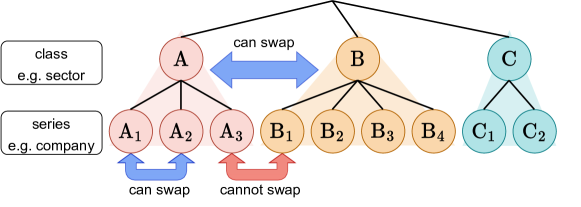
Figure 1: Hierarchical permutation

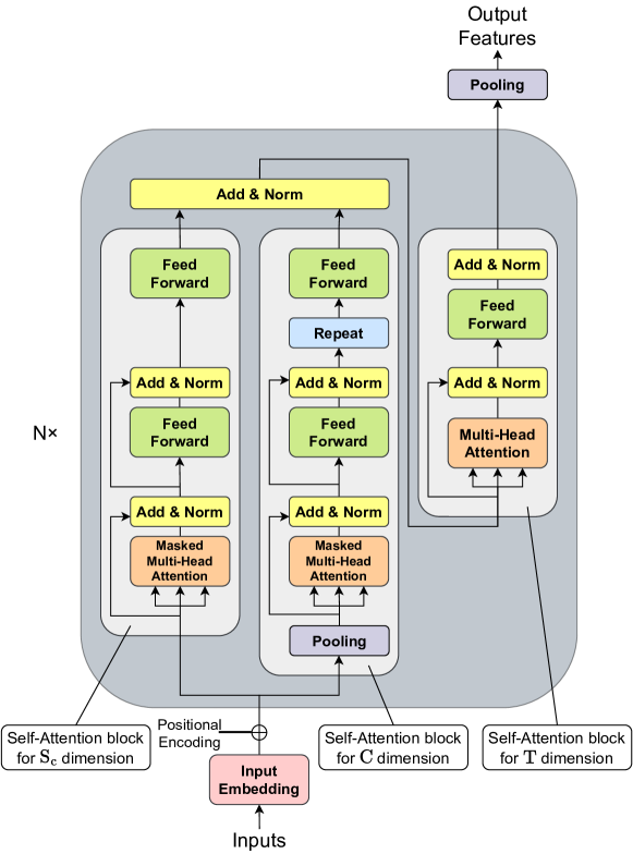
Figure 2: Feature extractor architecture

Algorithm 1 3D self-attention

1:  Input: $M\in\mathbb{R}^{C\times S_{c}\times T_{in}\times D_{model}}$

2:  

3:  /*  Self-Attention Block for $S_{c}$ Dimension     Curriculate $M^{S_{c}}\in\mathbb{R}^{C\times S_{c}\times T_{in}\times D_{model}}$ */

4:  for $c=1$ to $C$ do

5:     for $t=1$ to $T_{in}$ do

6:        $M^{S_{c}}_{c,\>:,\>t,\>:}\leftarrow\text{SelfAttForSc}(M_{c,\>:,\>t,\>:})$

7:     end for

8:  end for

9:  

10:  /*  Self-Attention Block for $C$ Dimension     Curriculate $M^{C}\in\mathbb{R}^{C\times S_{c}\times T_{in}\times D_{model}}$ */

11:  for $c=1$ to $C$ do

12:     $M^{P}_{c,\>:,\>:,\>:}\leftarrow\text{Pool}(M_{c,\>:,\>:,\>:})\in\mathbb{R}^{T_{in}\times D_{model}}$

13:  end for

14:  for $t=1$ to $T_{in}$ do

15:     $M^{P}_{:,\>t,\>:}\leftarrow\text{SelfAttForC}(M^{P}_{:,\>t,\>:})$

16:  end for

17:  for $s=1$ to $S_{c}$ do

18:     $M^{C}_{:,\>s,\>:,\>:}\leftarrow M^{P}$

19:  end for

20:  

21:  /*  Self-Attention Block for $T$ Dimension     Curriculate $M^{T}\in\mathbb{R}^{C\times S_{c}\times T_{in}\times D_{model}}$ */

22:  $M^{T}\leftarrow M^{S_{c}}+M^{C}$

23:  for $c=1$ to $C$ do

24:     for $s=1$ to $S_{c}$ do

25:        $M_{c,\>s,\>:,\>:}\leftarrow\text{SelfAttForT}(M_{c,\>s,\>:,\>:})$

26:     end for

27:  end for

28:  

29:  Output: $M^{T}\in\mathbb{R}^{C\times S_{c}\times T_{in}\times D_{model}}$

3.3 Model Overview

We can obtain the distribution that $Y$ follows by passing the input tensor $X$ through the Feature Extractor and Distribution Estimator proposed in this study. These proposed modules have the following properties.

• Capture hierarchical dependencies among series.

• Hierarchically permutation-equivariant and capable of handling the entry and exit of series accepting series set of arbitrary size.

• Outputs time-varying and diverse joint distributions.

3.4 Feature Extractor

The feature extractor is a stack of 3D self-attention layers shown in 2. Before passing to it, we classify the input tensor $X$ using the class information $\bm{c}$. If $S$ series are divided into $C$ classes and the number of series in the largest class is $S_{c}$, $X$ can be formatted into a tensor of $\mathbb{R}^{C\times S_{c}\times T_{in}\times D_{in}}$. Here, $X_{i,j}$ represents the observation of the series $j$ in class $i$. Note that $X_{i,j}$, where $j$ exceeds the number of series belonging to the class $i$, will not be referenced because it is information on a series that does not exist. After this, $\bm{c}$ is never used and never input to the model as a feature.
Then, $X$ is embedded into the in-model tensor $M\in\mathbb{R}^{C\times S_{c}\times T_{in}\times D_{model}}$, and then it is input into the 3D self-attention layer.

3.4.1 3D Self-Attention Layer

Algorithm. A 3D self-attention layer consists of blocks that take self-attention for intra-class ($S_{c}$), inter-class ($C$), and time ($T$) dimensions. The blocks for $S_{c}$ and $C$ are parallel, followed by the $T$ block. The algorithm is shown in 1, and line 3-8, 10-19, 21-27 corresponds $S_{c}$, $C$, and $T$ dimension block respectively. SelfAttForSc, SelfAttForC, and SelfAttForT are the self-attention functions for $S_{c}$, $C$, and $T$ dimensions respectively. When taking self-attention for $S_{c}$ dimension, we fix the class index and time, and then take self-attention among series in the class. When taking self-attention for $C$ dimension, first we compress class information (line 8-10), and then take self-attention among classes with fixing time (line 12-14). Finally, we repeat the self-attention output for $S_{c}$ dimension (line 15-17). When taking self-attention for $T$ dimension, we fix the class and series index, and then take self-attention among series in the class.

Properties. We can obtain hierarchical dependencies among the series by combining self-attention for $S_{c}$ and $C$ dimensions, and finally, by taking self-attention for $T$, we can capture complex time evolution considering the entire input. Furthermore, the entire 3D self-attention layer is hierarchically permutation-equivariant and accepts any size set of series as input. An explanation for this is provided below.

Self-Attention Block for $S_{c}$ Dimension. This block is permutation-equivariant for $C$ dimension and accepts any number of classes as input since the same process is applied to all the classes. As $S_{c}$ dimension is only subjected to self-attention, it is permutation-equivariant and can accept any number of series from the same class as input.

Self-Attention Block for $C$ Dimension. This block is permutation-equivariant for $S_{c}$ and accepts any number of series in a class as input since it only performs permutation-invariant compression and repeats for the $S_{c}$ dimension. Also, for the $C$ dimension, since it only considers self-attention, it is permutation-equivariant and accepts any number of classes as input.

Self-Attention Block for $T$ Dimension. This block is hierarchically permutation-equivariant and accepts any number of classes and series in a class as input because the same process is applied to all classes and series in a class for this calculation.

3.4.2 Post Process and Summary

The shape of tensor $M$ does not change in the 3D self-attention layer. After fusing $C$ and $S_{c}$ dimensions of $M$, we obtain the time-varying features for each series $Z=(Z_{1},\dots,Z_{S})\in\mathbb{R}^{S\times T_{out}\times D_{model}}$ by removing the padded portions and pooling for $T$ dimension. $Z$ is a feature that captures both the heterarchical dependencies among series and the temporal evolution of each series through 3D self-attention. Note that by removing the self-attention block for $C$ dimension from the 3D self-attention layer and considering all series in the same class, it becomes another proposed model HiPerformer-w/o-class that does not use class information. This model has a mere permutation-equivariance (not hierarchical) and can acquire relationships among series, and has the same properties as the full model.

3.5 Distribution Estimator

A distribution estimator is a mechanism that takes a feature $Z$ obtained with 3.4 as input and predicts a time-varying probability distribution that the target variable $Y$ follows. In particular, this study assumes that $Y_{:,\>t,\>d}$ follows a multidimensional normal distribution $\mathcal{N}(\mu_{:,t,d},\Sigma_{:,\>:,\>t,\>d})$, and output its mean $\mu\in\mathbb{R}^{S\times T_{out}\times D_{out}}$ and covariance matrix $\Sigma\in\mathbb{R}^{S\times S\times T_{out}\times D_{out}}$. The algorithm for calculating $\mu,\Sigma$ is described below.

3.5.1 Calculation of $\mu$

$\mu$ is calculated with a linear layer of $f_{\mu}:\mathbb{R}^{D_{model}}\to\mathbb{R}^{D_{out}}$, as in the following formula.

$$\mu=(f_{\mu}(Z_{1}),...,f_{\mu}(Z_{S}))^{T}\in\mathbb{R}^{S\times T_{out}\times D_{out}}$$ (1)

3.5.2 Calculation of $\Sigma$

Since the covariance matrix is a positive (semi)definite, the output $\Sigma_{:,\>:,\>t,\>d}$ here must also be positive definite. We have $D_{out}$ linear layers each of $f_{r}:\mathbb{R}^{D_{model}}\to\mathbb{R}^{D_{r}},\;f_{l}:\mathbb{R}^{D_{model}}\to\mathbb{R}^{D_{l}},\;f_{\sigma}:\mathbb{R}^{D_{model}}\to\mathbb{R}^{D_{\sigma}}$. Let the $d$-th ones be $f_{r_{d}}$, $f_{l_{d}}$, and $f_{\sigma_{d}}$ respectively, then $\Sigma_{i,j,t,d}$ is calculated as in the following equation.

$$\begin{split}\Sigma_{i,\>j,\>t,\>d}&=(r_{i,\>j,\>t,\>d}+l_{i,\>j,\>t,\>d})\sigma_{i,\>j,\>t,\>d}\\ where\;r_{i,\>j,\>t,\>d}&=k_{RBF}\left(f_{r_{d}}(Z_{i,\>t,\>:}),f_{r_{d}}(Z_{j,\>t,\>:})\right)\\ l_{i,\>j,\>t,\>d}&=k_{LIN}\left(f_{l_{d}}(Z_{i,\>t,\>:}),f_{l_{d}}(Z_{j,\>t,\>:})\right)\\ \sigma_{i,\>j,\>t,\>d}&=k_{LIN}\left(f_{\sigma_{d}}(Z_{i,\>t,\>:}),f_{\sigma_{d}}(Z_{j,\>t,\>:})\right)\end{split}$$ (2)

Here, $k_{RBF}(\bm{x},\bm{y})=\exp(\gamma\|\bm{x}-\bm{y}\|^{2}),\;k_{LIN}(\bm{x},\bm{y})=\bm{x}^{T}\bm{y}$, representing the RBF and linear kernels respectively. $\Sigma_{:,\>:,\>t,\>d}$ is positive definite because it is a Gram matrix of kernels combining positive definite kernels by sum and product. The RBF kernel can extract nonlinear relationships, but its value range is limited to $(0,1]$. Hence, it is combined with a linear kernel to improve its expressive power.

3.6 Training Strategy

We optimize the model to maximize the likelihood $\sum_{t}\sum_{d}\mathcal{N}(Y_{:,t,d}|\mu_{:,t,d},\Sigma_{:,\>:,\>t,\>d})$; that is, we can minimize the following negative log likelihood.

$$\mathcal{L}=\sum_{t}\sum_{d}-\log\mathcal{N}(Y_{:,t,d}|\mu_{:,t,d},\Sigma_{:,\>:,\>t,\>d})$$ (3)

Note that the negative log-likelihood of a multivariate normal distribution, $-\log\mathcal{N}(\bm{u}|\bm{v},W)$ is calculated as follows.

$$- \log\mathcal{N}(\bm{u}|\bm{v},W)$$ (4)

$$=\frac{1}{2}\left[D\log(2\pi)+\log|W|+(\bm{u}-\bm{v})^{T}W^{-1}(\bm{u}-\bm{v})\right]$$ (5)

4 Experiments

In this section, we validate the performance of the proposed method on two different tasks described in 2.2, multi-agent trajectory prediction, and hierarchical forecasting. For each task, first, we introduce datasets, evaluation metrics, and methods. Thereafter, we conduct evaluations.

4.1 Multi-Agent Trajectory Prediction

4.1.1 Datasets

We use one artificial dataset and one real-world dataset, where the series interact with each other.

Charged Dataset (Kipf et al., 2018) is an artificial dataset that records the motion of charged particles controlled by simple physical laws. Each scene contains five particles, each with a positive or negative charge. Particles with the same charge repel each other, and particles with different charges attract each other. The task is to predict the trajectory for the next 20 periods based on the trajectory and velocity for 80 periods. Subsequently, 50K, 10K, and 10K scenes of data are used for training, validation, and testing, respectively. In the proposed model, each particle is classified according to whether its charge is positive or negative.

NBA Dataset (Yue et al., 2014) is a dataset of National Basketball Association (NBA) games for the 2012–2013 season. Each scene has 10 players and 1 ball and the task is to predict the trajectory of the following 10 periods based on the historical trajectory and velocity for 40 periods. Here, 80000, 48299, and 13464 scenes of data are used for training, validation, and testing, respectively. The proposed model categorizes each series into three classes: ball, and the team to which it belongs.

4.1.2 Evaluation Metrics

To evaluate the accuracy of probabilistic forecasts, we evaluate the likelihood of the forecast distribution and the results of point forecasts.

Average displacement error (ADE) and final displacement error (FDE): ADE is the root mean squared error between the ground truth and predicted trajectories. FDE measures the root mean squared error between the ground truth final destination and the predicted final destination. For stochastic models, we report the minimum (and mean for one method) displacement error of all predicted trajectories/destinations. The lower values are preferred.

Negative log likelihood (NLL): It measures how plausible the ground truth is for the predicted distribution. For stochastic models, we report the mean NLL of all trajectories. We only report this metric on models that are trained with NLL or evidence lower bound (ELBO)  (Sohn et al., 2015). The lower values are preferred.

4.1.3 Methods

We adopt the following four methods　as baselines that utilize interactions among agents.

Fuzzy query attention (FQA) (Kamra et al., 2020) is a method that combines RNN with a module that acquires induced bias from the relative movements, intentions, and interactions of sequences.

Neural relational inference (NRI) (Kipf et al., 2018) represents interactions among agents as a potential graph from past trajectories and generates future trajectories as variational auto-encoders (VAEs) (Kingma and Welling, 2013).

Social-GAN (Gupta et al., 2018) is a traditional GAN-based method that effectively handles multimodality.

GRIN (Li et al., 2021) extracts latent representations that separate the intentions of each agent and the relationships between agents and generates trajectories considering high-level interactions between agents utilizing GATs (Velickovic et al., 2017). To the best of our knowledge, this is the state-of-the-art method in this dataset.

Next we explain about our proposed model HiPerformer.

HiPerformer. We compare aforesaid baselines with HiPerformer-prob, the full proposed model; HiPerformer-det, which is HiPerformer-prob without the covariance estimation described in 3.5.2 and only predicts trajectories; HiPerformer-w/o-class-prob, which is HiPerformer-prob without the self-attention block for $C$ dimension in 3.4.1; and HiPerformer-w/o-class-det, which is HiPerformer-w/o-class-prob without the covariance estimation. While HiPerformer-prob and HiPerformer-w/o-class-prob are trained with NLL, HiPerformer-det, and HiPerformer-w/o-class-det are trained with distance errors, such as mean absolute error (MAE) and mean square error (MSE). In this task, we use MAE. Also note that we never use class information for HiPerformer-w/o-class-prob and HiPerformer-w/o-class-det, as described in 3.4.2. We use SAB described in 2.3 when taking self-attention for $S_{c},C$ dimension.

A comparison of baselines with the proposed method is shown in 1.

Implementation Details. We implement our model using PyTorch  (Paszke et al., 2019). We stack two 3D self-attention layer, $D_{model}$ is 64, the number of heads for multi-head attention is 4, the batch size is 8 for Charged dataset and 64 for NBA dataset. We train our model using Adam optimizer  (Kingma and Ba, 2014) with learning rate $1\times 10^{-3}$. The results of baseline methods are from  (Li et al., 2021) except for GRIN. We train GRIN with parameters used in  (Li et al., 2021).

Table 1: Comparison of baselines and the proposed method. The $\triangle$ is added because DeepVAR+ and HierE2E estimate hierarchical dependency structures only with respect to sums, and HiPerformer is hierarchically permutation-equivariant, although full permutation-equivariance is not guaranteed.

Method	FQA	NRI	Social-GAN	DeepVAR	DeepVAR+	HierE2E	HiPerformer -w/o-class (Ours)	HiPerformer (Ours)
Probabilistic	$\times$	$\checkmark$	$\checkmark$	$\checkmark$	$\checkmark$	$\checkmark$	$\checkmark$	$\checkmark$
Inter-Series Hierarchical Dependencies	$\times$	$\times$	$\times$	$\times$	$\triangle$	$\triangle$	$\times$	$\checkmark$
Inter-Series Dependencies	$\checkmark$	$\checkmark$	$\checkmark$	$\checkmark$	$\checkmark$	$\checkmark$	$\checkmark$	$\checkmark$
Entry and Exit of Series	$\times$	$\times$	$\checkmark$	$\times$	$\times$	$\times$	$\checkmark$	$\checkmark$
Hierarchically-Permutation-Equivariant	$\times$	$\times$	$\times$	$\times$	$\times$	$\times$	$\times$	$\checkmark$
Permutation-Equivariant	$\times$	$\times$	$\checkmark$	$\times$	$\times$	$\times$	$\checkmark$	$\triangle$
No Class Information Needed	$\checkmark$	$\checkmark$	$\checkmark$	$\checkmark$	$\times$	$\times$	$\checkmark$	$\times$

Table 2: Performance comparison in multi-agent trajectory prediction. Non-generative methods have $\dagger$ after their names.　For GRIN and the proposed methods, we report the mean and standard deviation over five runs. The best results are in bold.

Dataset	Charged			NBA
Model	ADE	FDE	NLL	ADE	FDE	NLL
FQA$\dagger$	0.82	1.76	-	2.42	4.81	-
NRI-min	(0.63)	(1.30)	-	(2.10)	(4.56)	586.9
Social-GAN-min	(0.66)	(1.25)	-	(1.88)	(3.64)	-
GRIN-min	(0.53$\pm$0.01)	(1.10$\pm$0.02)	237.86$\pm$30.51	(1.73$\pm$0.03)	(3.67$\pm$0.08)	509.27$\pm$3.23
GRIN-mean	0.69$\pm$0.06	1.45$\pm$0.12		1.98$\pm$0.03	4.26$\pm$0.08
HiPerformer-w/o-class -det (Ours)$\dagger$	0.51$\pm$0.01	1.14$\pm$0.02	-	1.65$\pm$0.00	3.64$\pm$0.00	-
HiPerformer-det (Ours)$\dagger$	0.58$\pm$0.00	1.22$\pm$0.02	-	1.64$\pm$0.01	3.60$\pm$0.02	-
HiPerformer-w/o-class -prob (Ours)$\dagger$	0.44$\pm$0.00	1.05$\pm$0.00	-11.70$\pm$1.57	1.64$\pm$0.01	3.69$\pm$0.02	20.96$\pm$0.20
HiPerformer-prob (Ours)$\dagger$	0.52$\pm$0.01	1.18$\pm$0.01	2.9$\pm$3.48	1.65$\pm$0.00	3.68$\pm$0.01	21.14$\pm$0.26
AttT-det$\dagger$	0.63$\pm$0.01	1.37$\pm$0.02	-	1.83$\pm$0.00	4.06$\pm$0.00	-
AttT-prob$\dagger$	0.61$\pm$0.01	1.37$\pm$0.02	13.85$\pm$1.03	1.92$\pm$0.00	4.25$\pm$0.00	26.58$\pm$0.14

4.1.4 Quantitative Evaluation

Baseline Comparison. Results for the baseline and proposed methods are shown in 2. The methods with “min” at the end of the model name are those that generate predictions probabilistically, and we report the best ADE and FDE among them. For NLL, the average is reported. We generate 100 predictions for both datasets. While this metric is common for evaluating generative methods (Gupta et al., 2018; Mohamed et al., 2020; Li et al., 2021), we cannot simply compare it with the results of nongenerative methods such as FQA and proposed methods; it would be better to compare using mean or median instead of the minimum value, and we bracket the min-model metrics in 2. Therefore, for GRIN, the best-performing existing method, we report the average of the metrics for the generated predictions as “GRIN-mean.”

In the Charged dataset, HiPerformer-w/o-class-prob has the best performance for all metrics and all the proposed methods outperform the GRIN-mean results. Especially for NLL, HiPerformer-w/o-class-prob significantly exceeds baselines. In this experiment, HiPerformer-w/o-class, which does not use class information, outperformed HiPerformer, which attempts to acquire hierarchical dependencies among series using the class structure. This could be because the number of particles is small (5) and the relationships are simpler than those in the real-world dataset. Thus, HiPerformer-w/o-class could obtain richer information from other class particles using the raw data, rather than compressing each class information as in the 8-9 lines of 1.

For NBA, the proposed method also outperformed baselines in all indices. HiPerformer-det was best for ADE and FDE. HiPerformer-w/o-class-prob and HiPerformer-prob performed similarly, both significantly outperforming baselines for NLL.

Ablation Study. We conduct experiments to confirm the effectiveness of self-attention for $S_{c},C$ dimension to acquire inter-series dependencies. The results for AttT, which removes the self-attention block for $S_{c},C$ dimension from the full proposed model and takes self-attention for $T$ dimension only, are shown at the bottom of the 2. AttT-prob estimates the mean and covariance, while AttT-det predicts only the mean. Consistently, HiPerformer and HiPerformer-w/o-class outperforms AttT, indicating that self-attention for $S_{c},C$ dimension is effective in obtaining dependencies among series.

Remove Series. We investigated the performance of the proposed method on changes in the number of series using the NBA dataset. We created a new test dataset set by randomly removing some players from the original test dataset, and evaluated the trained models obtained in Baseline Comparison. A comparison of HiPerformer-w/o-class-prob and HiPerformer-prob is shown in the 3. For ADE, the difference between the two is small. On the other hand, for FDE and NLL, HiPerformer-prob is more robust against removing series, and tends to perform better than HiPerformer-w/o-class-prob as more players are removed. In particular, the difference between the two is large for NLL. From this, we can say that when the class imbalance is large or the number of series is small, the performance degradation can be mitigated by using the relationship among classes.

Table 3: Comparison of HiPerformer-w/o-class-prob and HiPerformer-prob performance in NBA dataset when tested with 0-4 players removed from team A and B, respectively. In order from the table above, ADE, FDE, and NLL are represented. Training was performed on all players’ data, and players were randomly removed during the test phase. The left side of each square is the result of HiPerformer-w/o-class-prob and the right side is the result of HiPerformer-prob. We report the mean and standard deviation over five runs. The better results are in bold.

	0	1	2	3	4
0	(1.64$\pm$0.01 - 1.65$\pm$0.00)	1.69$\pm$0.01 - 1.69$\pm$0.01	1.73$\pm$0.01 - 1.73$\pm$0.01	1.78$\pm$0.01 - 1.78$\pm$0.01	1.85$\pm$0.01 - 1.84$\pm$0.01
1	1.67$\pm$0.01 - 1.68$\pm$0.01	1.71$\pm$0.01 - 1.72$\pm$0.01	1.76$\pm$0.01 - 1.77$\pm$0.01	1.83$\pm$0.01 - 1.83$\pm$0.01	1.92$\pm$0.01 - 1.91$\pm$0.01
2	1.69$\pm$0.01 - 1.71$\pm$0.01	1.74$\pm$0.01 - 1.76$\pm$0.01	1.81$\pm$0.01 - 1.82$\pm$0.01	1.89$\pm$0.01 - 1.89$\pm$0.01	2.01$\pm$0.01 - 2.01$\pm$0.01
3	1.73$\pm$0.01 - 1.74$\pm$0.01	1.79$\pm$0.01 - 1.80$\pm$0.01	1.87$\pm$0.01 - 1.88$\pm$0.01	1.98$\pm$0.01 - 1.99$\pm$0.01	2.15$\pm$0.01 - 2.16$\pm$0.01
4	1.76$\pm$0.01 - 1.79$\pm$0.01	1.84$\pm$0.01 - 1.87$\pm$0.01	1.95$\pm$0.01 - 1.97$\pm$0.01	2.11$\pm$0.01 - 2.13$\pm$0.01	2.38$\pm$0.01 - 2.40$\pm$0.01
	0	1	2	3	4
0	(3.69$\pm$0.02 - 3.68$\pm$0.01)	3.78$\pm$0.02 - 3.76$\pm$0.01	3.87$\pm$0.02 - 3.84$\pm$0.01	3.98$\pm$0.02 - 3.94$\pm$0.01	4.13$\pm$0.02 - 4.07$\pm$0.01
1	3.73$\pm$0.02 - 3.72$\pm$0.01	3.82$\pm$0.02 - 3.80$\pm$0.01	3.93$\pm$0.02 - 3.90$\pm$0.01	4.06$\pm$0.02 - 4.02$\pm$0.01	4.25$\pm$0.02 - 4.19$\pm$0.01
2	3.76$\pm$0.02 - 3.76$\pm$0.01	3.86$\pm$0.02 - 3.85$\pm$0.01	3.99$\pm$0.02 - 3.97$\pm$0.01	4.16$\pm$0.02 - 4.13$\pm$0.01	4.41$\pm$0.02 - 4.35$\pm$0.01
3	3.81$\pm$0.02 - 3.81$\pm$0.01	3.93$\pm$0.02 - 3.93$\pm$0.01	4.09$\pm$0.02 - 4.08$\pm$0.01	4.31$\pm$0.02 - 4.29$\pm$0.01	4.65$\pm$0.02 - 4.61$\pm$0.01
4	3.86$\pm$0.02 - 3.87$\pm$0.01	4.01$\pm$0.02 - 4.02$\pm$0.01	4.22$\pm$0.02 - 4.22$\pm$0.02	4.53$\pm$0.02 - 4.52$\pm$0.02	5.06$\pm$0.02 - 5.02$\pm$0.02
	0	1	2	3	4
0	(20.96$\pm$0.20 - 21.14$\pm$0.26)	21.43$\pm$0.29 - 21.40$\pm$0.23	21.89$\pm$0.32 - 21.79$\pm$0.24	22.45$\pm$0.35 - 22.26$\pm$0.24	22.97$\pm$0.39 - 22.67$\pm$0.24
1	21.39$\pm$0.30 - 21.42$\pm$0.24	21.74$\pm$0.31 - 21.69$\pm$0.23	22.29$\pm$0.35 - 22.16$\pm$0.24	22.99$\pm$0.40 - 22.75$\pm$0.25	23.69$\pm$0.45 - 23.31$\pm$0.25
2	21.68$\pm$0.33 - 21.68$\pm$0.22	22.10$\pm$0.34 - 22.01$\pm$0.22	22.78$\pm$0.39 - 22.60$\pm$0.23	23.68$\pm$0.45 - 23.36$\pm$0.24	24.65$\pm$0.52 - 24.15$\pm$0.23
3	22.04$\pm$0.37 - 22.01$\pm$0.22	22.57$\pm$0.39 - 22.44$\pm$0.21	23.45$\pm$0.45 - 23.19$\pm$0.22	24.66$\pm$0.54 - 24.22$\pm$0.23	26.12$\pm$0.65 - 25.44$\pm$0.22
4	22.51$\pm$0.41 - 22.43$\pm$0.20	23.21$\pm$0.44 - 23.00$\pm$0.19	24.39$\pm$0.53 - 24.02$\pm$0.19	26.13$\pm$0.65 - 25.51$\pm$0.21	28.57$\pm$0.84 - 27.56$\pm$0.17

4.1.5 Qualitative Evaluation

The trajectory predictions in the NBA dataset are shown in 3. Looking at the attention scores among classes, we can see that a wide variety of information can be retrieved, with the top row showing more attention to Team B and the bottom row showing more attention to Team A. Next, take a look at the attention score of player A5 in the upper row. Here, A5 is the player with the ball, and since the enemy B4 is approaching, he is probably trying to pass the ball to a player on his side. Now, A5 is paying attention to A1, A2, and A4, and this may be because there are few enemy players around A1 and A2, and A4 is close to the goal. The proposed method is able to capture the complex relationships among real-world time series as described above.

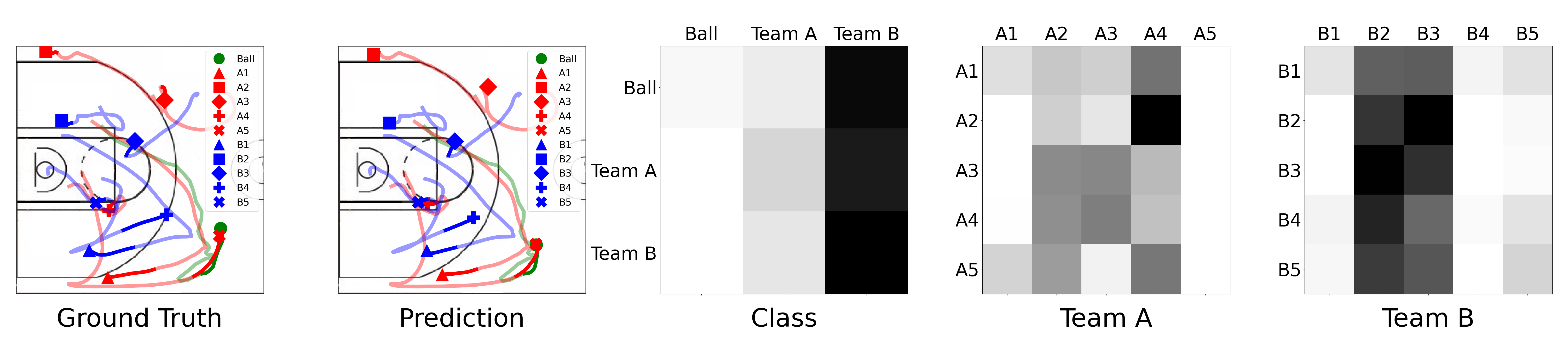
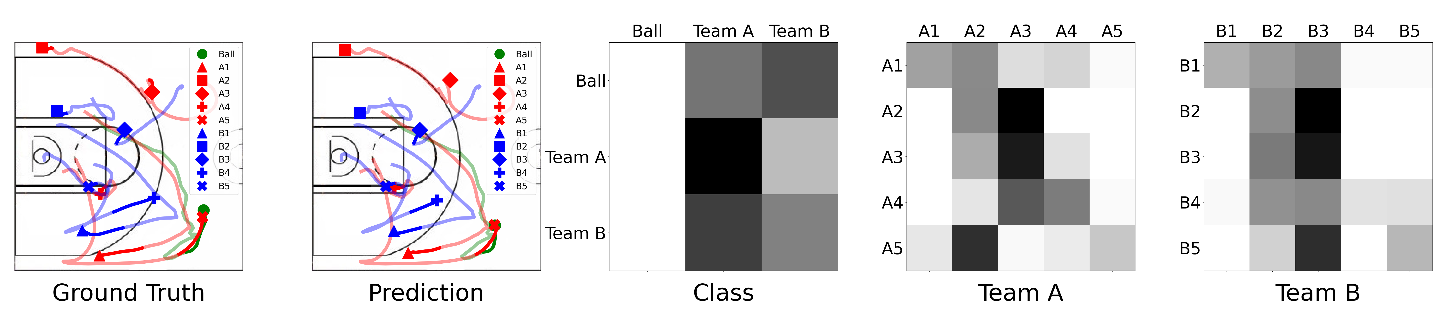
Figure 3: Trajectory prediction on NBA dataset. The left two figures are ground truth and predicted trajectories. Green represents a ball, red represents a player from Team A, and blue represents a player from Team B. The light line represents the 40-period trajectory of the input and the dark line represents the 10-period trajectory of the ground truth or prediction. The third figure from the left represents the atttention score among the classes, and the fourth and fifth figures represent the atttention score among the players of each team. Higher attention scores are in darker color. The upper and lower rows show the attention scores of different heads on the same input data.

4.2 Hierarchical Forecasting

Table 4: RMSE and NLL at each aggregation level. We report the mean and standard deviation for proposed method and best of baselines over 5 runs. The best results are in bold.

Metrics		RMSE				NLL
Dataset	Level	DeepVAR (not coherent)	DeepVAR+	HierE2E	HiPerformer (Ours)	DeepVAR (not coherent)	DeepVAR+	HierE2E	HiPerformer (Ours)
Labour	1	561.7 $\pm$ 59.2	629.0 $\pm$ 117.0	656.3 $\pm$ 151.5	4.58$\pm$2.05	13.11 $\pm$ 1.19	12.14 $\pm$ 3.12	14.64 $\pm$ 3.54	4.33$\pm$0.41
	2	104.5 $\pm$ 13.5	112.9 $\pm$ 15.3	112.5 $\pm$ 18.3	2.64$\pm$0.89	7.44 $\pm$ 0.95	7.79 $\pm$ 1.79	7.85 $\pm$ 1.23	3.88$\pm$0.55
	3	55.8 $\pm$ 6.5	57.0 $\pm$ 7.7	57.4 $\pm$ 8.9	1.92$\pm$0.63	6.49 $\pm$ 0.81	6.25 $\pm$ 1.19	6.52 $\pm$ 0.89	3.58$\pm$0.37
	4	31.4 $\pm$ 3.5	31.9 $\pm$ 3.4	32.62 $\pm$ 4.55	1.57$\pm$0.45	4.79 $\pm$ 0.36	4.81 $\pm$ 0.56	5.14 $\pm$ 0.49	4.28$\pm$0.32
Traffic	1	41.90 $\pm$ 8.09	22.40 $\pm$ 8.44	22.59 $\pm$ 15.71	3.10$\pm$2.26	5.19 $\pm$ 0.15	4.65 $\pm$ 0.18	4.77 $\pm$ 0.36	3.96$\pm$0.84
	2	24.79 $\pm$ 8.16	14.66 $\pm$ 1.98	15.13 $\pm$ 5.70	2.21$\pm$1.59	4.65 $\pm$ 0.31	4.20 $\pm$ 0.08	4.19 $\pm$ 0.25	3.50$\pm$0.67
	3	17.35 $\pm$ 3.98	10.70 $\pm$ 3.89	9.82 $\pm$ 2.29	1.56$\pm$1.12	4.28 $\pm$ 0.41	3.92 $\pm$ 0.22	3.71 $\pm$ 0.18	3.43$\pm$0.77
	4	1.46 $\pm$ 0.08	1.44 $\pm$ 0.05	1.47 $\pm$ 0.03	0.29$\pm$0.12	1.65 $\pm$ 0.14	1.57 $\pm$ 0.07	1.44 $\pm$ 0.12	3.99$\pm$1.35
Wiki	1	11088 $\pm$ 6717	11721 $\pm$ 7688	4125 $\pm$ 2483	204.73$\pm$175.54	11.05 $\pm$ 0.44	11.50 $\pm$ 0.36	9.88 $\pm$ 0.35	8.84$\pm$1.48
	2	3107 $\pm$ 941	4188 $\pm$ 1218	3855 $\pm$ 340	158.68$\pm$91.94	9.57 $\pm$ 0.20	10.03 $\pm$ 0.24	12.66 $\pm$ 1.34	8.13$\pm$0.45
	3	2773 $\pm$ 60	3082 $\pm$ 335	2851 $\pm$ 187	142.58$\pm$36.72	9.69 $\pm$ 0.17	9.28 $\pm$ 0.12	12.85 $\pm$ 0.92	8.12$\pm$0.43
	4	2737 $\pm$ 178	2943 $\pm$ 264	2769 $\pm$ 151	145.90$\pm$37.89	9.45 $\pm$ 0.46	9.21 $\pm$ 0.12	15.56 $\pm$ 1.68	8.11$\pm$0.43
	5	931 $\pm$ 22	978 $\pm$ 65	932 $\pm$ 26	96.60$\pm$22.26	8.02 $\pm$ 0.20	8.17 $\pm$ 0.43	9.61 $\pm$ 0.84	8.26$\pm$0.24

The data used in 4.1 have three levels from bottom to top, namely, bottom, class, and root levels, and we make predictions and evaluations only for the bottom-level or agent. In contrast, at this time, we will conduct experiments on data with four or more levels, where the feature values of the upper-level series are the sum of those of the lower-level series. Furthermore, we perform prediction and evaluation for the bottom-level series and the aggregate series at each level.

4.2.1 Datasets

For all datasets, given data for $T$ periods, to make predictions for $\tau$ periods, we use $1:T-2\tau$ data in training, perform validation at $T-2\tau+1:T-\tau$, and test at $T-\tau+1:T$. This is a setting following existing studies using this dataset (Rangapuram et al., 2021; Olivares et al., 2021), and we also adopt the same forecasting period $\tau$.

Labour (Australian Bureau of Statistics, 2021) is monthly Australian employment data from Feb. 1978 to Dec. 2020. We construct a 57-series hierarchy using categories such as region, gender, and employment status, as in  (Rangapuram et al., 2021). In this data, $T$ is 514 and $\tau$ is 8. It has four levels, and we classify the bottom-level series at the second level from the top in the proposed method.

Traffic (Cuturi, 2011; Dua and Graff, 2017) records the occupancy of 963 car lanes in the San Francisco Bay Area freeways from January 2008 to March 2009. We obtain daily observations for one year and generate a 207-series hierarchy using the same aggregation method as in previous hierarchical forecasting research (Ben Taieb and Koo, 2019; Rangapuram et al., 2021). In these data, $T$ is 366 and $\tau$ is 1. It has four levels, and we classify the bottom-level series at the second level from the top in the proposed method.

Wiki consists of daily views of 145K Wikipedia articles from July 2015 to December 2016. We follow previous studies (Ben Taieb and Koo, 2019; Rangapuram et al., 2021; Olivares et al., 2021) to select 150 bottom series and generate a 199-series hierarchy. In these data, $T$ is 366 and $\tau$ is 1. It has five levels, and we classify the bottom-level series at the fourth level from the top in the proposed method.

4.2.2 Evaluation Metrics

As with 4.1.2, to evaluate the accuracy of probabilistic forecasts, we evaluate the likelihood of the forecast distribution with NLL and the results of point forecasts with RMSE. For both evaluation metrics, we calculate averages for each aggregation level.

4.2.3 Methods

We adopt as baselines the following three recent methods that have been successful in this task.

DeepVAR  (Salinas et al., 2019) extends the VAM to deep learning with RNN, a probabilistic forecasting method that can determine the parameters of the distribution that a multivariate time series follows. Hierarchical consistency is not guaranteed.

DeepVAR+  (Rangapuram et al., 2021) adds hierarchical consistency to DeepVAR’s prediction with respect to sums.

HierE2E  (Rangapuram et al., 2021) first estimates the distribution followed by the target set of series and then projects the predictions sampled from it to be hierarchically consistent with respect to the sums. To the best of our knowledge, this is the state-of-the-art method for this task.

Next we explain about our proposed model HiPerformer.

HiPerformer. We use full proposed model HiPerformer, which we call HiPerformer-prob in 4.1. We first select one of the aggregation levels as the class level and classify the bottom-level series based on it. Subsequently, we obtain the feature values of each bottom-level series by feature extractor in 3.4. Here, the feature values of the aggregate series are the sum of the feature values of the bottom-level series in the sub-tree with itself as the root. Currently, we have the feature values of all the series including the aggregate series and predict the distribution using the distribution estimator in 3.5. We use ISAB described in 2.3 to reduce computational cost when taking self-attention for $S_{c},C$ dimension, and the dimension of inducing points  (Lee et al., 2019) is set to 20.

A comparison of baselines with the proposed method is shown in 1.

Implementation Details. We use the same parameters in 4.2.3 for our model, except for batch size. We set the batch size 8 for labour, 4 for traffic, and 4 for wiki. We train baseline models with parameters used in  (Rangapuram et al., 2021).

4.2.4 Evaluation

The results are shown in the 4. The proposed model outperforms the baseline on all datasets and metrics except for the bottom-level NLL of Traffic and Wiki. Particularly, the improvement in performance on RMSE is remarkable, indicating that the proposed method captures the hierarchical consistency for sums well. The NLL is often markedly improved compared to the baseline, demonstrating the proposed method’s capacity to generate diverse joint distributions while preserving the hierarchical dependency structure, even for multilevel data.

5 Conclusion

We proposed two prediction models HiPerformer and HiPerformer-w/o-class that can be applied to a set of time series in which new entries and exits of series can occur. The first model is HiPerformer that can capture hierarchical dependencies among series. To achieve this property, we defined the new concepts of hierarchical permutation and hierarchical permutation-equivariance and showed that HiPerformer is hierarchically permutation-equivariant. The second model is HiPerformer-w/o-class that is permutation-equivariant and captures the relationships among series without using class information. Both models can output various joint distributions, including time-varying covariances. These proposed models achieve state-of-the-art performance on synthetic and real-world datasets. From this, we indicate that using its hierarchical dependency structure is effective in forecasting classified time series sets.

Acknowledgements
This work was partially supported by JST AIP Acceleration Research JPMJCR20U3, Moonshot R&D Grant Number JPMJPS2011, CREST Grant Number JPMJCR2015, JSPS KAKENHI Grant Number JP19H01115 and Basic Research Grant (Super AI) of Institute for AI and Beyond of the University of Tokyo.

References

- Sukcharoen and Leatham [2016] Kunlapath Sukcharoen and David J Leatham. Dependence and extreme correlation among us industry sectors. Studies in Economics and Finance, 33(1):26–49, 2016.
- Zaheer et al. [2017] Manzil Zaheer, Satwik Kottur, Siamak Ravanbakhsh, Barnabas Poczos, Russ R Salakhutdinov, and Alexander J Smola. Deep sets. In Advances in Neural Information Processing Systems, volume 30, pages 3391–3401, 2017.
- Cho et al. [2014] Kyunghyun Cho, Bart van Merrienboer, Çaglar Gülçehre, Fethi Bougares, Holger Schwenk, and Yoshua Bengio. Learning phrase representations using RNN encoder-decoder for statistical machine translation. CoRR, abs/1406.1078, 2014. URL http://arxiv.org/abs/1406.1078.
- Khandelwal et al. [2018] Urvashi Khandelwal, He He, Peng Qi, and Dan Jurafsky. Sharp nearby, fuzzy far away: How neural language models use context. arXiv preprint arXiv:1805.04623, 2018.
- Vaswani et al. [2017] Ashish Vaswani, Noam Shazeer, Niki Parmar, Jakob Uszkoreit, Llion Jones, Aidan N Gomez, Ł ukasz Kaiser, and Illia Polosukhin. Attention is all you need. In Advances in Neural Information Processing Systems, volume 30, pages 5998–6008, 2017.
- Li et al. [2019] Shiyang Li, Xiaoyong Jin, Yao Xuan, Xiyou Zhou, Wenhu Chen, Yu-Xiang Wang, and Xifeng Yan. Enhancing the locality and breaking the memory bottleneck of transformer on time series forecasting. Advances in neural information processing systems, 32, 2019.
- Zhou et al. [2021] Haoyi Zhou, Shanghang Zhang, Jieqi Peng, Shuai Zhang, Jianxin Li, Hui Xiong, and Wancai Zhang. Informer: Beyond efficient transformer for long sequence time-series forecasting. In Proceedings of the AAAI Conference on Artificial Intelligence, volume 35, pages 11106–11115, 2021.
- Wu et al. [2021] Haixu Wu, Jiehui Xu, Jianmin Wang, and Mingsheng Long. Autoformer: Decomposition transformers with auto-correlation for long-term series forecasting. Advances in Neural Information Processing Systems, 34:22419–22430, 2021.
- Zhou et al. [2022] Tian Zhou, Ziqing Ma, Qingsong Wen, Xue Wang, Liang Sun, and Rong Jin. Fedformer: Frequency enhanced decomposed transformer for long-term series forecasting. arXiv preprint arXiv:2201.12740, 2022.
- Liu et al. [2021] Shizhan Liu, Hang Yu, Cong Liao, Jianguo Li, Weiyao Lin, Alex X Liu, and Schahram Dustdar. Pyraformer: Low-complexity pyramidal attention for long-range time series modeling and forecasting. In International Conference on Learning Representations, 2021.
- Wu et al. [2020] Sifan Wu, Xi Xiao, Qianggang Ding, Peilin Zhao, Ying Wei, and Junzhou Huang. Adversarial sparse transformer for time series forecasting. Advances in neural information processing systems, 33:17105–17115, 2020.
- Goodfellow et al. [2020] Ian Goodfellow, Jean Pouget-Abadie, Mehdi Mirza, Bing Xu, David Warde-Farley, Sherjil Ozair, Aaron Courville, and Yoshua Bengio. Generative adversarial networks. Communications of the ACM, 63(11):139–144, 2020.
- Scarselli et al. [2008] Franco Scarselli, Marco Gori, Ah Chung Tsoi, Markus Hagenbuchner, and Gabriele Monfardini. The graph neural network model. IEEE transactions on neural networks, 20(1):61–80, 2008.
- Bai et al. [2020] Lei Bai, Lina Yao, Can Li, Xianzhi Wang, and Can Wang. Adaptive graph convolutional recurrent network for traffic forecasting. Advances in neural information processing systems, 33:17804–17815, 2020.
- Defferrard et al. [2016] Michaël Defferrard, Xavier Bresson, and Pierre Vandergheynst. Convolutional neural networks on graphs with fast localized spectral filtering. Advances in neural information processing systems, 29, 2016.
- Kipf and Welling [2016] Thomas N Kipf and Max Welling. Semi-supervised classification with graph convolutional networks. arXiv preprint arXiv:1609.02907, 2016.
- Zhao et al. [2021] Hang Zhao, Jiyang Gao, Tian Lan, Chen Sun, Ben Sapp, Balakrishnan Varadarajan, Yue Shen, Yi Shen, Yuning Chai, Cordelia Schmid, et al. Tnt: Target-driven trajectory prediction. In Conference on Robot Learning, pages 895–904. PMLR, 2021.
- Salzmann et al. [2020] Tim Salzmann, Boris Ivanovic, Punarjay Chakravarty, and Marco Pavone. Trajectron++: Dynamically-feasible trajectory forecasting with heterogeneous data. In European Conference on Computer Vision, pages 683–700. Springer, 2020.
- Mangalam et al. [2020] Karttikeya Mangalam, Yang An, Harshayu Girase, and Jitendra Malik. From Goals, Waypoints & Paths To Long Term Human Trajectory Forecasting, 2020.
- Leon and Gavrilescu [2021] Florin Leon and Marius Gavrilescu. A review of tracking and trajectory prediction methods for autonomous driving. Mathematics, 9(6):660, 2021.
- Kretzschmar et al. [2014] Henrik Kretzschmar, Markus Kuderer, and Wolfram Burgard. Learning to predict trajectories of cooperatively navigating agents. In 2014 IEEE international conference on robotics and automation (ICRA), pages 4015–4020. IEEE, 2014.
- Schmerling et al. [2018] Edward Schmerling, Karen Leung, Wolf Vollprecht, and Marco Pavone. Multimodal probabilistic model-based planning for human-robot interaction. In 2018 IEEE International Conference on Robotics and Automation (ICRA), pages 3399–3406. IEEE, 2018.
- Felsen et al. [2017] Panna Felsen, Pulkit Agrawal, and Jitendra Malik. What will happen next? forecasting player moves in sports videos. In Proceedings of the IEEE international conference on computer vision, pages 3342–3351, 2017.
- Li et al. [2021] Longyuan Li, Jian Yao, Li Wenliang, Tong He, Tianjun Xiao, Junchi Yan, David Wipf, and Zheng Zhang. Grin: Generative relation and intention network for multi-agent trajectory prediction. Advances in Neural Information Processing Systems, 34:27107–27118, 2021.
- Velickovic et al. [2017] Petar Velickovic, Guillem Cucurull, Arantxa Casanova, Adriana Romero, Pietro Lio, and Yoshua Bengio. Graph attention networks. stat, 1050:20, 2017.
- Rangapuram et al. [2021] Syama Sundar Rangapuram, Lucien D Werner, Konstantinos Benidis, Pedro Mercado, Jan Gasthaus, and Tim Januschowski. End-to-end learning of coherent probabilistic forecasts for hierarchical time series. In International Conference on Machine Learning, pages 8832–8843. PMLR, 2021.
- Olivares et al. [2021] Kin G Olivares, O Nganba Meetei, Ruijun Ma, Rohan Reddy, Mengfei Cao, and Lee Dicker. Probabilistic hierarchical forecasting with deep poisson mixtures. arXiv preprint arXiv:2110.13179, 2021.
- Lee et al. [2019] Juho Lee, Yoonho Lee, Jungtaek Kim, Adam Kosiorek, Seungjin Choi, and Yee Whye Teh. Set transformer: A framework for attention-based permutation-invariant neural networks. In Proceedings of the 36th International Conference on Machine Learning, volume 97, pages 3744–3753, 2019.
- Kipf et al. [2018] Thomas Kipf, Ethan Fetaya, Kuan-Chieh Wang, Max Welling, and Richard Zemel. Neural relational inference for interacting systems. In International Conference on Machine Learning, pages 2688–2697. PMLR, 2018.
- Yue et al. [2014] Yisong Yue, Patrick Lucey, Peter Carr, Alina Bialkowski, and Iain Matthews. Learning fine-grained spatial models for dynamic sports play prediction. In 2014 IEEE international conference on data mining, pages 670–679. IEEE, 2014.
- Sohn et al. [2015] Kihyuk Sohn, Honglak Lee, and Xinchen Yan. Learning structured output representation using deep conditional generative models. Advances in neural information processing systems, 28, 2015.
- Kamra et al. [2020] Nitin Kamra, Hao Zhu, Dweep Kumarbhai Trivedi, Ming Zhang, and Yan Liu. Multi-agent trajectory prediction with fuzzy query attention. Advances in Neural Information Processing Systems, 33:22530–22541, 2020.
- Kingma and Welling [2013] Diederik P Kingma and Max Welling. Auto-encoding variational bayes. arXiv preprint arXiv:1312.6114, 2013.
- Gupta et al. [2018] Agrim Gupta, Justin Johnson, Li Fei-Fei, Silvio Savarese, and Alexandre Alahi. Social gan: Socially acceptable trajectories with generative adversarial networks. In Proceedings of the IEEE conference on computer vision and pattern recognition, pages 2255–2264, 2018.
- Paszke et al. [2019] Adam Paszke, Sam Gross, Francisco Massa, Adam Lerer, James Bradbury, Gregory Chanan, Trevor Killeen, Zeming Lin, Natalia Gimelshein, Luca Antiga, et al. Pytorch: An imperative style, high-performance deep learning library. Advances in neural information processing systems, 32, 2019.
- Kingma and Ba [2014] Diederik P Kingma and Jimmy Ba. Adam: A method for stochastic optimization. arXiv preprint arXiv:1412.6980, 2014.
- Mohamed et al. [2020] Abduallah Mohamed, Kun Qian, Mohamed Elhoseiny, and Christian Claudel. Social-stgcnn: A social spatio-temporal graph convolutional neural network for human trajectory prediction. In Proceedings of the IEEE/CVF Conference on Computer Vision and Pattern Recognition, pages 14424–14432, 2020.
- Australian Bureau of Statistics [2021] 2020 Australian Bureau of Statistics. Australian bureau of statistics. labour force, australia, dec 2020., 2021. URL https://www.abs.gov.au/statistics/labour/employment-and-unemployment/labour-force-australia/dec-2020. Accessed on 01.18.2023.
- Cuturi [2011] Marco Cuturi. Fast global alignment kernels. In Proceedings of the 28th international conference on machine learning (ICML-11), pages 929–936, 2011.
- Dua and Graff [2017] D. Dua and Graff. Uci machine learning repository, 2017. URL http://archive.ics.uci.edu/ml. Accessed on 01.18.2023.
- Ben Taieb and Koo [2019] Souhaib Ben Taieb and Bonsoo Koo. Regularized regression for hierarchical forecasting without unbiasedness conditions. In Proceedings of the 25th ACM SIGKDD International Conference on Knowledge Discovery & Data Mining, pages 1337–1347, 2019.
- Salinas et al. [2019] David Salinas, Michael Bohlke-Schneider, Laurent Callot, Roberto Medico, and Jan Gasthaus. High-dimensional multivariate forecasting with low-rank gaussian copula processes. Advances in neural information processing systems, 32, 2019.