Prox-DBRO-VR: A Unified Analysis on Decentralized Byzantine-Resilient Composite Stochastic Optimization with Variance Reduction and Non-Asymptotic Convergence Rates

Abstract

Decentralized Byzantine-resilient stochastic gradient algorithms resolve efficiently large-scale optimization problems in adverse conditions, such as malfunctioning agents, software bugs, and cyber attacks. This paper aims to handle a class of general composite optimization problems over multi-agent cyber-physical systems (CPSs), with the existence of an unknown number of Byzantine agents. Based on the proximal mapping method, variance-reduced (VR) techniques, and a norm-penalized approximation strategy, we propose a decentralized Byzantine-resilient and proximal-gradient algorithmic framework, dubbed Prox-DBRO-VR, which achieves an optimization and control goal using only local computations and communications. To reduce asymptotically the variance generated by evaluating the noisy stochastic gradients, we incorporate two localized variance-reduced techniques (SAGA and LSVRG) into Prox-DBRO-VR to design Prox-DBRO-SAGA and Prox-DBRO-LSVRG. By analyzing the contraction relationships among the gradient-learning error, robust consensus condition, and optimal gap, theoretical results demonstrate that both Prox-DBRO-SAGA and Prox-DBRO-LSVRG, with a well-designed constant (resp., decaying) step-size, converge linearly (resp., sub-linearly) inside an error ball around the optimal solution to the optimization problem under standard assumptions. The trade-off between convergence accuracy and the number of Byzantine agents in both linear and sub-linear cases is characterized. In simulation, the effectiveness and practicability of the proposed algorithms are manifested via resolving a decentralized sparse machine-learning problem over multi-agent CPSs under various Byzantine attacks.

I Introduction

I-A Literature Review

Decentralized optimization has seen extensive research and notable progress in the field of machine learning [1, 2, 3], smart grids [4], cooperative control [5], and uncooperative games [6]. Decentralized optimization algorithms have the advantages of high-efficiency for massive-scale optimization problems, good scalability over large-scale intelligent systems, and a lower cost in short-distance communications.

With the rapid expansion of multi-agent CPSs, there are unavoidable security issues in the process of optimization and control, such as poisoning data, software bugs, malfunctioning devices, and cyber attacks [7, 8]. All these issues in the course of multi-agent optimization and control are generalized as a node-level problem model, namely Byzantine problems [9], while the malfunctioning or compromised agents are called Byzantine agents. Byzantine agents are able to stop the existing notable decentralized optimization algorithms [10, 11, 2, 5, 12, 13, 14, 6, 15, 4, 16, 1, 17] from achieving the optimal solution to the optimization problem [18], or even cause disagreement and divergence [19]. For example, if an honest agent is attacked and controlled by adversaries, the attacker can manipulate the agent to send misleadingly falsified information to its different reliable neighboring agents at each iteration. This can easily deter reliable agents from achieving convergence, and even the consensus is impeded if one Byzantine agent chooses to send different misleading messages to different reliable neighbors. Therefore, researchers have been concentrating on designing decentralized resilient algorithms [20, 21, 22, 23, 24, 25, 26, 27, 28] to alleviate or counteract the negative impact caused by Byzantine agents. In fact, there are various approaches to guarantee decentralized Byzantine resilience. One popular line is to combine various screening or filtration techniques with decentralized algorithms. To name a few, ByRDiE [29] requires that each agent at every iteration discards a subset of the largest and smallest messages in the received information, which is followed by a coordinate gradient descent step. One imperfection of ByRDiE is its expensive computational overhead and low efficiency in dealing with large-scale optimization problems due to the implementation of one-coordinate-at-one-iteration update. Hence, BRIDGE [23] combines respectively four screening techniques including coordinate-wise trimmed-mean, coordinate-wise median, Krum function, and a combination of Krum and coordinate-wise trimmed mean, with decentralized gradient descent (DGD) [30] to devise a Byzantine-resilient algorithmic framework. However, these four screening mechanisms either suffer from a high computational complexity or impose extra restrictions on the number of neighbors and the network topology. Follow-up literature [31] incorporates a self-centered clipping technique (adapted from the centered clipping [32]) into DGD to not only realize Byzantine resilience, but resolve a category of general non-convex objective functions. However, the decentralized algorithm proposed in [31] assumes that each agent has the prior knowledge of global parameters, for instance, the subset of Byzantine agents. This may be impractical in real large-scale CPSs, since the information exchange is only available in a decentralized manner. Another literature [18] designs a two-stage technique to filter out the Byzantine attacks, which can work over multi-agent CPSs with an arbitrary quantity of Byzantine agents while any clairvoyant knowledge of the identities of Byzantine agents is not required. Recent work [26] systematically analyzes the challenges on two critical points, i.e., doubly-stochastic weight matrix and consensus, in the development of decentralized Byzantine-resilient methods. Based on the analysis, a screening-based robust aggregation rule, dubbed (IOS), is designed in [26], which achieves Byzantine resilience and a controllable convergence error relied on the assumptions of bounded inner (node-level noisy stochastic gradients) and outer (network-level aggregated gradients) variations.

All of the aforementioned decentralized Byzantine algorithms [29, 23, 31, 18, 26] achieve Byzantine resilience via adopting various screening or filtering techniques. Nevertheless, the screening or filtration-based methods may not only impose restrictions on the minimum number of neighboring agents, but incur at least an additional computational cost of $\mathcal{O}\left({n\left|{{\mathcal{N}_{i}}}\right|}\right)$ ($n$ and ${\mathcal{N}_{i}}$ denote the dimension of single data sample and the number of neighboring agents of the reliable agent $i$, respectively) to each reliable agent $i$ at each iteration (see [23, TABLE II]). This could be prohibitively expensive if the optimization problem is high-dimensional (machine learning or deep learning tasks) or the multi-agent CPSs are large-scale. One possible solution to avoid introducing extra computational costs for decentralized Byzantine-resilient optimization is developed by RSA [28], which combines an $a$-norm-penalized ($a\geq 1$) approximation method with the stochastic sub-gradient descent method to realize robust aggregation in a distributed fashion. [27] is a decentralized extension of RSA [28]. Via integrating with a noise-shuffle strategy, [33] extends [28] to distributed federated learning, which enhances users’ differential privacy. However, both RSA [28] and the literature [27, 33] establish only sub-linear convergence rates of the proposed algorithms, which are rather slow and have huge potential to be accelerated. A recent decentralized Byzantine-resilient algorithm DECEMBER [34] accelerates the convergence rate via incorporating two variance-reduced techniques. Although DECEMBER realizes simultaneously Byzantine resilience and linear convergence, it is still confined to resolving optimization problems with only a single smooth objective function.

I-B Motivations

All aforementioned decentralized Byzantine-resilient methods [29, 28, 27, 33, 23, 31, 18, 26, 34] are not available to handling optimization problems with the existence of any non-smooth objective, which is indispensable in many practical applications, such as sparse machine learning [35, 36], model predictive control [5], and energy resource coordination [12]. On the other hand, despite that there are various decentralized algorithms [37, 35, 38, 36, 12, 3] providing different insights and tactics to resolve the composite optimization problem, they all fail to consider any possible security issues over CPSs, which renders the reliable agents under the algorithmic framework of [35, 38, 36, 12] easily misled by Byzantine failures and vulnerable to Byzantine attacks. Therefore, to close this gap, this paper focuses on studying a category of composite optimization problems in the presence of Byzantine agents, where the local objective function associated with each agent consists of both smooth and non-smooth parts. In a nutshell, the study on decentralized Byzantine-resilient composite stochastic optimization is non-trivial, which features the main motivation of this paper.

I-C Contributions

1. This paper designs a decentralized Byzantine-resilient and proximal-gradient algorithmic framework, dubbed Prox-DBRO-VR, to resolve a class of composite (smooth + non-smooth) optimization problems over multi-agent CPSs under the worst case of Byzantine attacks. The worst case indicates that the number of Byzantine agents is unlimited and any information relevant to their identities is not necessarily known by reliable agents. To reduce the expensive per-iteration computational cost in decentralized Byzantine-resilient batch-gradient methods [29, 23, 39, 40, 20], we incorporate the localized versions of two variance-reduced techniques SAGA [41] and LSVRG [42], into Prox-DBRO-VR, to propose two decentralized Byzantine-resilient stochastic gradient algorithms, namely Prox-DBRO-SAGA and Prox-DBRO-LSVRG. Owing to the employment of the variance-reduced techniques, Prox-DBRO-SAGA and Prox-DBRO-LSVRG reduce asymptotically the variance incurred by the local stochastic gradients, which also eliminates the bounded-variance assumption required by [43, 28, 27, 14, 26].

2. In contrast to recent works [39, 23, 25, 26, 24, 34, 40, 20], this papers considers a more general composite optimization problem model with local non-smooth objective functions. This superiority also brings challenges in theoretical analysis, which has been addressed by exploring the contraction properties of proximal operators over decentralized Byzantine-resilient optimization. Different with [28, 27, 33, 34], a unified convergence analysis is conducted in this paper to obtain more intuitive and complete theoretical results, including both a sub-linear convergence rate (with a smaller convergence error) and a linear convergence rate (with a larger convergence error), which provides in-depth knowledge of the trade-off between convergence speed and convergence accuracy. Furthermore, the uncoordinated parameter setup is considered in algorithm development, i.e., uncoordinated penalty parameters of Prox-DBRO-VR and uncoordinated triggered probabilities of Prox-DBRO-LSVRG, which not only allows each agent to decide independently their own parameters, but contributes to attaining a more complete convergence result.

3. The screening or filtration-based Byzantine-resilient methods, such as [19, 23, 29, 39, 18, 25, 26, 24], may impose a rigorous assumption on the number of neighboring agents of the reliable agents or the network topology, which may be impractical in the large-scale CPSs with a complex system structure. To eliminate this requirement, Prox-DBRO-SAGA and Prox-DBRO-LSVRG adopt a generalized penalized-norm approximation method to realize Byzantine resilience. Moreover, both Prox-DBRO-SAGA and Prox-DBRO-LSVRG achieve Byzantine resilience without incurring any additional costs in contrast to the decentralized Byzantine-resilient methods [19, 23, 29, 25, 18, 26, 24] that result in either prohibitively expensive screening or observation costs, especially when facing large-scale or high-dimensional optimization problems. Besides, the theoretical analysis of Prox-DBRO-SAGA and Prox-DBRO-LSVRG only requires one potential connected network among reliable agents, which is more relaxed than the observation-based methods [40, 20] relying on trust observations and assumptions of sufficiently connected networks and bounded malicious information.

I-D Organization

We provide the remainder of the paper in this part. Section II presents the basic notation, problem statement, problem reformulation, and setup of its robust variant. The connection of the proposed algorithms with existing methods and the algorithm development are elaborated in Section III. Section IV details the convergence results of the proposed algorithms. Case studies on decentralized learning problems with various Byzantine attacks to illustrate the effectiveness and performance of the proposed algorithms are carried out in Section V. Section VI concludes the paper and states our future direction. Some detailed derivations are placed to Appendix for coherence.

II Preliminaries

II-A Basic Notation

Throughout the paper, we assume all vectors are column vectors if there is no other specified.

Symbols	Definitions
${\mathbb{R}}$, ${{\mathbb{R}}^{n}}$, ${{\mathbb{R}}^{m\times n}}$	the set of real numbers, $n$-dimensional column real vectors, $m\times n$ real matrices, respectively
${I_{n}}$	the $n\times n$ identity matrix
${0_{n}}$	an $n$-dimensional column vector with all-zero elements
$1_{m}$	an $m$-dimensional column vector with all-one elements
${\cdot^{\top}}$	transpose of any matrices or vectors
${\rm{diag}}\left\{\nu\right\}$	a diagonal matrix with all the elements of vector $\nu\in{\mathbb{R}^{n}}$ laying on its main diagonal
$X\leq Y$	each element in $Y-X$ is nonnegative, where $X$ and $Y$ are two vectors or matrices with same dimensions
$\tilde{x}\otimes\tilde{y}$	the Kronecker product of vectors $\tilde{x}$ and $\tilde{y}$
$\left|\cdot\right|$	the operator to represent the absolute value of a constant or the cardinality of a set
$\left\|\nu\right\|_{a}$	either the $a$-norm of $\nu\in{\mathbb{R}^{n}}$ equivalent to ${\left({\sum\nolimits_{i=1}^{n}{{{\left|{{\nu_{i}}}\right|}^{a}}}}\right)^{\frac{1}{a}}}$, $a\geq 1$, or its induced matrix norm.
${\lambda_{\min}}\left(X\right)$	the minimum nonzero singular value of any matrix $X$
${\lambda_{\max}}\left(X\right)$	the maximum singular value of any matrix $X$

TABLE I: Basic notations.

For arbitrary three vectors $\tilde{x},\tilde{y},\tilde{z}\in\mathbb{R}^{n}$, a positive scalar $a$ and a closed, proper, convex function, $g:{\mathbb{R}^{n}}\to\mathbb{R}$, the proximal operator is defined as: ${\mathbf{prox}}_{{a,g}}\left\{\tilde{x}\right\}=\arg{\min_{\tilde{y}\in\mathbb{R}^{n}}}\left\{{g\left(\tilde{y}\right)+\frac{1}{{2a}}{{\left\|{\tilde{y}-\tilde{x}}\right\|}_{2}^{2}}}\right\}$; let $\partial g\left(\tilde{x}\right)$ denote the sub-differential of the proper, closed and convex function $g:{\mathbb{R}^{n}}\to\mathbb{R}$ at $\tilde{x}$, such that

$$\partial g\left(\tilde{x}\right)=\left\{{\tilde{y}|\forall\tilde{z}\in{\mathbb{R}^{n}},\;g\left(\tilde{x}\right)+\left\langle{\tilde{y},\tilde{z}-\tilde{x}}\right\rangle\leq g\left(\tilde{z}\right)}\right\};$$

let ${{\partial_{\tilde{x}}}g\left(\tilde{x}\right)}$ denote the sub-gradient of non-smooth convex function $g$ at $\tilde{x}$. The remaining basic notations of this paper are summarized in Table I.

II-B Problem Statement

A network of $m$ agents connect with each other over an undirected network $\mathcal{G}=\left({\mathcal{R}\cup\mathcal{B},\mathcal{E}}\right)$, where $\mathcal{R}$ ($0\leq\left|\mathcal{R}\right|\leq m$) and $\mathcal{B}$ indicate the sets of reliable and Byzantine agents, respectively, and $\mathcal{E}$ represents the set of undirected communication edges among all agents. The mutual target of all reliable agents is to minimize (min) a general decentralized composite optimization problem as follows:

$$\mathop{\min}\limits_{\tilde{x}\in{\mathbb{R}^{n}}}\sum\limits_{i\in\mathcal{R}}{{f_{i}}\left({\tilde{x}}\right)+{g}\left({\tilde{x}}\right)},$$ (1)

where $\tilde{x}$ is the decision variable, and ${f_{i}}:{\mathbb{R}^{n}}\to\mathbb{R}$ and ${g}:{\mathbb{R}^{n}}\to\mathbb{R}$, $i\in\mathcal{R}$, are two different objective functions. The local objective function $f_{i}$ can be further decomposed as ${f_{i}}\left({\tilde{x}}\right)=\sum\nolimits_{l=1}^{{q_{i}}}{f_{i}^{l}\left({\tilde{x}}\right)}/q_{i}$, while $g$ features a shared non-smooth part similar to literature [36, 35, 38]. We assume that the optimal solution to (1) exists, denoted by $\tilde{x}^{*}$, and the local sample set associated with agent $i$ as ${\mathcal{Q}_{i}}=\left\{{1,2,\ldots,{q_{i}}}\right\}$, $\forall i\in\mathcal{R}$. To specify the problem, we need to make the following assumptions.

Assumption 1

(Convexity and Smoothness).
a) For $i\in\mathcal{R}$, the local objective function $f_{i}$ is $\mu_{i}$-strongly convex, and the local component objective function $f_{i}^{l}$, is $L_{i}$-smooth, $\forall l\in{\mathcal{Q}_{i}}$, i.e., $\forall{\tilde{x}},{\tilde{z}}\in{\mathbb{R}^{n}}$,

$${\mu_{i}}\left\|{\tilde{x}-\tilde{z}}\right\|_{2}^{2}\leq{\left({\nabla{f_{i}}\left({\tilde{x}}\right)-\nabla{f_{i}}\left({\tilde{z}}\right)}\right)^{\top}}\left({\tilde{x}-\tilde{z}}\right),$$ (2a)

$${\left\|{\nabla f_{i}^{l}\left({\tilde{x}}\right)-\nabla f_{i}^{l}\left({\tilde{z}}\right)}\right\|_{2}}\leq L_{i}{\left\|{\tilde{x}-\tilde{z}}\right\|_{2}},$$ (2b)

where $\mu:=\mathop{\min}\nolimits_{i\in\mathcal{R}}\left\{{{\mu_{i}}}\right\}$ and $L:={\max_{i\in\mathcal{R}}}\left\{{{L_{i}}}\right\}$, with ${\kappa_{f}}:=L/\mu$;
b) The objective function $g$ is convex and not necessarily smooth.

Remark 1

Assumption 1-a) is standard in recent literature [16, 15, 13, 12, 14, 10]. According to [44, Chapter 3], we know that $0<\mu\leq L$, which indicates $\kappa_{f}\geq 1$. Moreover, in view of (2b), it is not difficult to verify that the local objective function $f_{i}$, $i\in\mathcal{R}$, is $L$-smooth as well. Under Assumption 1, the optimal solution $\tilde{x}^{*}$ to (1) exists uniquely. The consideration of the possibly non-smooth term $g$ is meaningful, which finds substantial applications in various fields, such as the standard 1-norm regularization term in sparse machine learning [35, 36], the non-smooth indicator function in model predictive control [5], and the non-differentiable emission cost in energy resource coordination over smart grids [12].

The following assumption is also standard in recent literature [28, 27, 33].

Assumption 2

(Network Connectivity). All reliable agents form a static network, denoted as $\left({\mathcal{R},{\mathcal{E}_{\mathcal{R}}}}\right)$, which is bidirectionally connected.

II-C Problem Reformulation

To guarantee all reliable agents reach a consensus at the optimal solution, we need to reformulate (1) into an equivalent consensus problem. To achieve this goal, a global decision vector $x=\left[{x_{1}^{\top},x_{2}^{\top},\ldots,x_{\left|\mathcal{R}\right|}^{\top}}\right]^{\top}\in{\mathbb{R}^{\left|\mathcal{R}\right|n}}$ with $\left|\mathcal{R}\right|$ local copies of the decision variable $\tilde{x}$, is introduced, subject to (s.t.) the consensus constraint ${x_{i}}={x_{j}},\left({i,j}\right)\in\mathcal{E}$. Therefore, it is natural to rewrite (2) as

$$\mathop{\min}\limits_{x\in{\mathbb{R}^{\left|\mathcal{R}\right|n}}} F\left(x\right)+G\left(x\right),\hfill$$ (3)

$${\text{s}}{\text{.t}}{\text{. }}{x_{i}} ={x_{j}},\left({i,j}\right)\in{\mathcal{E}_{\mathcal{R}}},\hfill$$

where $F\left(x\right):=\sum\nolimits_{i\in\mathcal{R}}{f_{i}\left({{x_{i}}}\right)}$ and $G\left(x\right):=\sum\nolimits_{i\in\mathcal{R}}{g\left({{x_{i}}}\right)}$.

II-D Robust Consensus Problem Setup

To enhance the robustness of the consensual aggregation process, we extend a scalar-valued consensus technique designed in [45] to its vector-valued domain. We can solve for the globally optimal solution ${x^{*}}$ of (3) via the following norm-penalized approximation

$${x^{*}}:=\arg\mathop{\min}\limits_{x}\sum\limits_{i\in\mathcal{R}}{\left({{f_{i}}\left({{x_{i}}}\right)+g\left({{x_{i}}}\right)+{\phi_{i}}\sum\limits_{j\in{\mathcal{R}_{i}}}{{{\left\|{{x_{i}}-{x_{j}}}\right\|}_{a}}}}\right)},$$ (4)

where $a\geq 1$, and $\phi_{i}$ is the local uncoordinated penalty parameter associated with each reliable agent $i$, $\forall i\in\mathcal{R}$. The introduction of the total-variation norm penalty provides a resilient replacement of the consensus constraint, i.e., the controllable distance between $x_{i}$ and $x_{j}$. The distance is controlled by the uncoordinated penalty parameter $\phi_{i}$, which means that a larger $\phi_{i}$ can bring a small gap between $x_{i}$ and $x_{j}$, $\left({i,j}\right)\in{\mathcal{E}_{\mathcal{R}}}$. To a certain extent, (1) can be considered as a soft relaxation of (4), because the former tolerates the dissimilarity among agents, for instance, the disagreement between reliable agents and Byzantine agents. The equivalence between the norm-penalized approximation problem (4) and the original optimization problem (1) is proved in Theorem 1.

III Algorithm Development

III-A Connection with Existing Works

Lian et al. in [46] design a decentralized stochastic gradient descent algorithm, namely DPSGD, to resolve efficiently the transformed optimization problem (3), in an ideal situation. The ideal situation fails to consider the presence of any malfunctioning or malicious agents, which may not be avoided in practical applications [24, 23, 47, 26, 22, 20, 9, 21]. We next find out the reason why DPSGD cannot be applied directly to solving (3) when there are Byzantine agents in the network, and then seek out a feasible improvement, based on DPSGD, to maintain Byzantine resilience. We first recap the updates of the generalized DPSGD as follows:

$${{\bar{x}}_{i,k}}={x_{i,k}}-{\alpha_{k}}{\nabla f_{i}\left({{x_{i,k}}}\right)},$$ (5a)

$${x_{i,k+1}}=\sum\limits_{j\in{\mathcal{N}_{i}}\cup\left\{i\right\}}{{w_{ij}}{{\bar{x}}_{j,k}}},$$ (5b)

where ${{\cal N}_{i}}={{\cal R}_{i}}\cup{{\cal B}_{i}}$, $\alpha_{k}$ denotes a constant or decaying step-size, ${\nabla f\left({{x_{i,k}}}\right)}$ is the local batch gradient, ${w_{ij}}$ is the $i$-th row and $j$-th column element of a doubly stochastic weight matrix, meeting $\sum\nolimits_{j\in{{\cal N}_{i}}}{{w_{ij}}}=\sum\nolimits_{j\in{{\cal N}_{i}}}{{w_{ji}}}=1$. If there is a Byzantine agent $o$ with one reliable neighbor $i$, ${{\tilde{x}}_{io,k}}$ could be an incorrect or misleading information (depending on whether agent $o$ is out of action or manipulated by adversaries), to its reliable neighboring agents, at $k$-th iteration. Then, ${x_{i,k+1}}$ can be arbitrarily deviate from its true model, if Byzantine agent $o$ is manipulated, since the adversary may send a maliciously falsifying message to agent $i$. For instance, Byzantine agent $o$, $o\in{{\cal B}_{i}}$, can blow $x_{i,k+1}$ up to infinity through transmitting continually a vector with infinite elements to its reliable neighbor $i$. Another example is that Byzantine agent $o$ can deter all reliable agents from achieving consensus at iteration $k$, via sending various values $\tilde{x}_{io,k}$ to its different reliable neighboring agents $i\in{\mathcal{R}_{o}}$. The main reason for the above mentioned issues comes from the fact that the aggregation step (5b) is rather vulnerable to Byzantine problems. In fact, similar problems also prevail in decentralized work [12, 10, 43, 1, 16, 13, 14, 15, 11, 2]. Therefore, the SGD family contains two important extensions, RSA [28] and [27], both of which achieve Byzantine resilience based on a robust consensus method [45]. [27] is a decentralized extension of RSA [28]. The theoretical analysis of both RSA [28] and [27] is based on a bounded-variance assumption on the local stochastic gradient. With this assumption and the other standard assumptions (see [27] for details), the sequence ${\left\{{{x_{k}}}\right\}_{k\geq 0}}$ generated by the decentralized algorithm proposed in [27] takes a convergent form of

$$\mathbb{E}\left[{\left\|{{x_{k+1}}-{1_{\left|\mathcal{R}\right|}}\!\otimes\!{\tilde{x}^{*}}}\right\|_{2}^{2}}\right]\leq \left({1-\eta{\alpha_{k}}}\right)\mathbb{E}\left[{\left\|{{x_{k}}-{1_{\left|\mathcal{R}\right|}}\!\otimes\!{\tilde{x}^{*}}}\right\|_{2}^{2}}\right]$$ (6)

$$+\alpha_{k}^{2}{\Delta_{0}}+{\alpha_{k}}{\Delta_{1}},$$

where $\eta$ is a positive constant satisfying $0<\eta{\alpha_{k}}<1$, ${\Delta_{0}}:=\sum\nolimits_{i\in\mathcal{R}}{32n{\phi^{2}}{{\left|{{\mathcal{R}_{i}}}\right|}^{2}}}+4n{\phi^{2}}{\left|{{\mathcal{B}_{i}}}\right|^{2}}+2\sigma_{i}^{2}$ (${\sigma_{i}}>0$ is the bounded variance yielded by the biased evaluation of the local batch gradients) and ${\Delta_{1}}:=\sum\nolimits_{i\in\mathcal{R}}{n{\phi^{2}}{{\left|{{\mathcal{B}_{i}}}\right|}^{2}}/\gamma}$. Based on (6), one can establish either a sub-linear convergence rate of a convergent error determined by the number of Byzantine agents, or a linear convergence rate with a convergent error determined jointly by the number of Byzantine agents and reliable agents, together with the bounded variance ${\sigma_{i}}$. In fact, this bounded variance ${\sigma_{i}}$ exists commonly in recent literature, such as [43, 28, 27, 14]. Therefore, this paper aims to reduce asymptotically this bounded variance in the linear convergence result and discard the bounded-variance assumption as well. Inspired by the recent exploration of decentralized variance-reduced stochastic gradient algorithms diffusion-AVRG [2], S-DIGing [15], GT-SAGA/GT-SVRG [11], GT-SARAH [1] and Push-LSVRG-UP [16] that seek the solution to the optimization problem under an ideal Byzantine-free situation, we consider introducing two popular localized variance-reduction techniques SAGA [41] and LSVRG [42] to reduce asymptotically the variance arising in the course of evaluating the noisy stochastic gradients.

III-B A General Algorithmic Framework

Based on the above analysis, we propose a decentralized Byzantine-resilient stochastic-gradient algorithmic framework in Algorithm 1 to resolve (4) in the presence of Byzantine agents.

Algorithm 1 Prox-DBRO-VR Framework

0:  Each reliable agent $i$, $i\in\mathcal{R}$, initializes with an arbitrary starting point $x_{i,0}\in{\mathbb{R}^{n}}$, a well-designed constant or decaying step-size $\alpha_{k}>0$, and the proper uncoordinated penalty parameters ${{\phi_{i}}}>0$, $\forall i\in\mathcal{R}$.

1:  for all $k=0,1,2,\ldots$ do

2:     Each reliable agent $i$, $i\in\mathcal{R}$, sends its current local model ${x_{i,k}}$ to its neighbors $j\in{\mathcal{N}_{i}}$ and receives the reliable information ${x_{j,k}}$ or malicious information ${z_{ij,k}}$ from its neighbors $j\in{\mathcal{N}_{i}}$.

3:     Each reliable agent $i$, $i\in\mathcal{R}$, evaluates the local stochastic gradient $r_{i,k}$.

4:     Each reliable agent $i$, $i\in\mathcal{R}$, updates an intermediate variable according to the robust local stochastic gradient descent step:

$${\bar{x}_{i,k}}={x_{i,k}}-{\alpha_{k}}r_{i,k}-{\alpha_{k}}{\phi_{i}}\sum\limits_{j\in{\mathcal{N}_{i}}}{{\partial_{{x_{i}}}}{{\left\|{{x_{i,k}}-v_{ij,k}}\right\|}_{a}}},$$

with ${v_{ij,k}}=\left\{\begin{gathered}{x_{j,k}},{\text{if}}\;j\in{\mathcal{R}_{i}}\lx@algorithmic@hfill\\ {z_{ij,k}},{\text{if}}\;j\in{\mathcal{B}_{i}}\lx@algorithmic@hfill\\ \end{gathered}\right..$

5:     Each reliable agent $i$, $i\in\mathcal{R}$, updates its current local model according to the local proximal mapping step:

$${x_{i,k+1}}=\mathop{\arg\min}\limits_{\tilde{x}\in{\mathbb{R}^{n}}}\left\{{g\left({\tilde{x}}\right)+\frac{1}{{2{\alpha_{k}}}}{{\left\|{\tilde{x}-{{\bar{x}}_{i,k}}}\right\|}_{2}^{2}}}\right\}.$$

6:  end for

Remark 2

The Byzantine resilience of Prox-DBRO-VR is attained by adopting the robust consensus aggregation based on total variation, which is initially studied in [45]. The literature [28, 33] extends this strategy to handling distributed federated learning problems, and [27] studies it in a decentralized manner. However, all these works [28, 27, 33] not only rely on a bounded-variance assumption in theoretical analysis, but establish slower sub-linear convergence rates. Thus, the most important goal of designing Prox-DBRO-VR is to achieve linear convergence and removes the bounded-variance assumption, which can be attained with the aid of VR techniques.

III-C Prox-DBRO-SAGA and Prox-DBRO-LSVRG

We introduce the localized version of two popular centralized VR techniques, SAGA [41] and LSVRG [42], into Prox-DBRO-VR, to develop Prox-DBRO-SAGA and Prox-DBRO-LSVRG. The detailed updates of Prox-DBRO-SAGA and Prox-DBRO-LSVRG are presented in Algorithms 2-3, respectively.

Algorithm 2 Prox-DBRO-SAGA

0:  Each reliable agent $i$, $i\in\mathcal{R}$, initializes the same parameters and starting points according to Algorithm 1, and auxiliary variables $u_{i,1}^{l}=u_{i,0}^{l}={x_{i,0}},\forall l\in\mathcal{Q}_{i}$, together with gradient tables $\left\{{\nabla f_{i}^{l}\left({u_{i,0}^{l}}\right)}\right\}_{l=1}^{{q_{i}}}$ additionally.

1:  for all $k=0,1,2,\ldots$ do

2:     Each reliable agent $i$, $i\in\mathcal{R}$, exchanges information according to Step 2 in Algorithm 1.

3:     Each reliable agent $i$, $i\in\mathcal{R}$, selects uniformly a random sample with index $s_{i,k}$ from the set $\mathcal{Q}_{i}$ and evaluates the lcoal stochastic gradient

$${r_{i,k}^{u}}\!=\!\nabla f_{i}^{{s_{i,k}}}\left({{x_{i,k}}}\right)-\nabla f_{i}^{{s_{i,k}}}\left({u_{i,k}^{{s_{i,k}}}}\right)\!+\frac{1}{{{q_{i}}}}\sum\limits_{l=1}^{{q_{i}}}\!\!{\nabla f_{i}^{l}\left({u_{i,k}^{l}}\right)}.$$

4:     Each reliable agent $i$, $i\in\mathcal{R}$, takes $u_{i,k+1}^{s_{i,k}}={x_{i,k}}$ and replaces $\nabla f_{i}^{{s_{i,k}}}\left({u_{i,k+1}^{s_{i,k}}}\right)$ by $\nabla f_{i}^{{s_{i,k}}}\left({{x_{i,k}}}\right)$ in the corresponding position of the gradient table, while keeps $\nabla f_{i}^{l}\left({u_{i,k+1}^{l}}\right)=\nabla f_{i}^{l}\left({u_{i,k}^{l}}\right)$, $l\in{\mathcal{Q}_{i}}\backslash\left\{{{s_{i,k}}}\right\}$.

5:     Each reliable agent $i$, $i\in\mathcal{R}$, updates its current model according to Steps 4-5 in Algorithm 1.

6:  end for

Algorithm 3 Prox-DBRO-LSVRG

0:  Each reliable agent $i$, $i\in\mathcal{R}$, initializes the same parameters and starting points according to Algorithm 1, and an auxiliary variable ${w_{i,0}}={x_{i,0}}$ additionally.

1:  for all $k=0,1,2,\ldots$ do

2:     Each reliable agent $i$, $i\in\mathcal{R}$, exchanges information according to Step 2 in Algorithm 1.

3:     Each reliable agent $i$, $i\in\mathcal{R}$, selects uniformly a random sample with index $s_{i,k}$ from the set $\mathcal{Q}_{i}$ and evaluates the local stochastic gradient

$${r_{i,k}^{w}}=\nabla f_{i}^{{s_{i,k}}}\left({{x_{i,k}}}\right)-\nabla f_{i}^{{s_{i,k}}}\left({{w_{i,k}}}\right)+\frac{1}{{{q_{i}}}}\sum\limits_{l=1}^{{q_{i}}}{\nabla f_{i}^{l}\left({{w_{i,k}}}\right)}.$$

4:     Each reliable agent $i$, $i\in\mathcal{R}$, takes $w_{i,k+1}={x_{i,k}}$ with an uncoordinated triggered probability $p_{i}$ and keeps $w_{i,k+1}={w_{i,k}}$ with the probability $1-p_{i}$.

5:     Each reliable agent $i$, $i\in\mathcal{R}$, updates its current model according to Steps 4-5 of Algorithm 1.

6:  end for

Remark 3

Note that all steps in Prox-DBRO-SAGA and Prox-DBRO-LSVRG, together with Prox-DBRO-VR, are executed in parallel among all reliable agents. It is also worthwhile to mention that the expected cost in evaluating the stochastic gradient under Prox-DBRO-LSVRG is at least double that of Prox-DBRO-SAGA at every iteration. However, this computational advantage of Prox-DBRO-SAGA is at the expense of an expensive storage cost of ${\cal O}\left({n{q_{i}}}\right)$ for each agent $i$ owing to the employment of the gradient table, while Prox-DBRO-LSVRG does not incur extra storage to save the local batch gradients. Therefore, adopting either Prox-DBRO-SAGA or Prox-DBRO-LSVRG in practice involves a trade-off between per-iteration computational cost and storage. Users can also implement Prox-DBRO-VR via incorporating other categories of VR techniques based on their customized needs.

IV Convergence Analysis

For the simplicity of notation, we denote ${{\mathcal{F}_{k}}}$ as the filter of the history with respect to the dynamical system generated by the sequence $\left\{{s_{k}^{i}}\right\}_{k\geq 0}^{i=1,2,\ldots,\left|\mathcal{R}\right|}$, and the conditional expectation $\mathbb{E}\left[{{s_{k}}|{\mathcal{F}_{k}}}\right]$ is shortly denoted by ${\mathbb{E}_{k}}\left[\cdot\right]$ in the sequel analysis. To facilitate the subsequent analysis, we give the sequel definitions.

$${x_{k}}:= {\left[{x_{1,k}^{\top},\ldots,x_{\left|\mathcal{R}\right|,k}^{\top}}\right]^{\top}}\in{\mathbb{R}^{\left|\mathcal{R}\right|n}},$$

$${r_{k}}:= {\left[{r_{1,k}^{\top},\ldots,r_{\left|\mathcal{R}\right|,k}^{\top}}\right]^{\top}}\in{\mathbb{R}^{\left|\mathcal{R}\right|n}},$$

$$\nabla F\left({{x_{k}}}\right):= {\left[{\nabla{f_{1}}{{\left({{x_{1,k}}}\right)}^{\top}},\ldots,\nabla{f_{\left|\mathcal{R}\right|}}{{\left({{x_{\left|\mathcal{R}\right|,k}}}\right)}^{\top}}}\right]^{\top}}\in{\mathbb{R}^{\left|\mathcal{R}\right|n}},$$

$${\partial_{x}}G\left({{x_{k}}}\right):= \left[{\partial_{{x_{1}}}}g{{\left({{x_{1,k}}}\right)}^{\top}},\ldots,{{\partial_{{x_{\left|\mathcal{R}\right|}}}}g{{\left({{x_{\left|\mathcal{R}\right|,k}}}\right)}^{\top}}}\right]^{\top}\!\in\!{\mathbb{R}^{\left|\mathcal{R}\right|n}},$$

$$\chi\left({{x_{k}}}\right):= \sum\limits_{i\in\mathcal{R}}{{\phi_{i}}\sum\limits_{j\in{\mathcal{R}_{i}}}{{{\left\|{{x_{i,k}}-{x_{j,k}}}\right\|}_{a}}}}\in{\mathbb{R}},$$

$$\delta\left({{x_{k}}}\right):= \sum\limits_{i\in\mathcal{R}}{{\phi_{i}}\sum\limits_{j\in{\mathcal{B}_{i}}}{{{\left\|{{x_{i,k}}-{z_{ij,k}}}\right\|}_{a}}}}\in{\mathbb{R}},$$

$${\partial_{{x_{i}}}}\chi\left({{x_{i,k}}}\right):= {\phi_{i}}\sum\limits_{j\in{\mathcal{R}_{i}}}{{\partial_{{x_{i}}}}{{\left\|{{x_{i,k}}-{x_{j,k}}}\right\|}_{a}}}\in{\mathbb{R}^{n}},$$

$${\partial_{x}}\chi\left({{x_{k}}}\right):= {\left[{{\partial_{{x_{1}}}}\chi{{\left({{x_{1,k}}}\right)}^{\top}},\ldots{\partial_{{x_{\left|\mathcal{R}\right|}}}}\chi{{\left({{x_{\left|\mathcal{R}\right|,k}}}\right)}^{\top}}}\right]^{\top}}\!\in\!{\mathbb{R}^{\left|\mathcal{R}\right|n}},$$

$${\partial_{{x_{i}}}}\delta\left({{x_{i,k}}}\right):= {\phi_{i}}\sum\limits_{j\in{\mathcal{R}_{i}}}{{\partial_{{x_{i}}}}{{\left\|{{x_{i,k}}-{z_{ij,k}}}\right\|}_{a}}}\in{\mathbb{R}^{n}},$$

$${\partial_{x}}\delta\left({{x_{k}}}\right):= {\left[{{\partial_{{x_{1}}}}\delta{{\left({{x_{1,k}}}\right)}^{\top}},\ldots,{\partial_{{x_{\left|\mathcal{R}\right|}}}}\delta{{\left({{x_{\left|\mathcal{R}\right|,k}}}\right)}^{\top}}}\right]^{\top}}\!\in\!{\mathbb{R}^{\left|\mathcal{R}\right|n}}.$$

Based on these definitions, we next provide briefly a compact form of Prox-DBRO-VR for the subsequent convergence analysis as follows:

$${\bar{x}_{k}}={x_{k}}-{\alpha_{k}}\left({r_{k}}+{\partial_{x}}\chi\left({{x_{k}}}\right){+{\partial_{x}}\delta\left({{x_{k}}}\right)}\right),$$ (7a)

$${x_{k+1}}={\mathbf{prox}}{{}_{{\alpha_{k}},G}}\left\{{{{\bar{x}}_{k}}}\right\}.$$ (7b)

IV-A Auxiliary Results

Inspired by the unified analysis framework for centralized stochastic gradient descent methods in [48], we introduce the following two lemmas. To begin with, we define respectively two sequences for Prox-DBRO-SAGA and Prox-DBRO-LSVRG in the following. For Prox-DBRO-SAGA, we define

$$t_{i,k}^{u}:=\frac{1}{{{q_{i}}}}\sum\limits_{l=1}^{{q_{i}}}{{f_{i}^{l}\left({u_{i,k}^{l}}\right)-f_{i}^{l}\left({{{\tilde{x}}^{*}}}\right)-\nabla f_{i}^{l}{{\left({{{\tilde{x}}^{*}}}\right)}^{\top}}\left({u_{i,k}^{l}-{{\tilde{x}}^{*}}}\right)}}.$$

For Prox-DBRO-LSVRG, we define

$$t_{i,k}^{w}:=\frac{1}{{{q_{i}}}}\sum\limits_{l=1}^{{q_{i}}}{{f_{i}^{l}\left({{w_{i,k}}}\right)-f_{i}^{l}\left({{{\tilde{x}}^{*}}}\right)-\nabla f_{i}^{l}{{\left({{{\tilde{x}}^{*}}}\right)}^{\top}}\left({{w_{i,k}}-{{\tilde{x}}^{*}}}\right)}}.$$

Note that both sequences ${\left\{{t_{i,k}^{u}}\right\}_{i\in\mathcal{R},k\geq 0}}$ and ${\left\{{t_{i,k}^{w}}\right\}_{i\in\mathcal{R},k\geq 0}}$ are non-negative according to the convexity of the local component function ${f_{i}^{l}}$, $l\in\mathcal{Q}_{i}$. For the sequel analysis, we define respectively the gradient-learning quantities $t_{k}^{u}:=\sum\nolimits_{i\in\mathcal{R}}{t_{i,k}^{u}}$ and $t_{k}^{w}:=\sum\nolimits_{i\in\mathcal{R}}{t_{i,k}^{w}}$ for Prox-DBRO-SAGA and Prox-DBRO-LSVRG, the largest and smallest number of local samples ${q_{\min}}:={\min_{i\in\mathcal{R}}}{q_{i}}$ and ${q_{\max}}:={\max_{i\in\mathcal{R}}}{q_{i}}$, the minimum and maximum triggered probabilities ${p_{\min}}:={\min_{i\in\mathcal{R}}}{p_{i}}$ and ${p_{\max}}:={\max_{i\in\mathcal{R}}}{p_{i}}$, while ${\kappa_{q}}:={q_{\max}}/{q_{\min}}\geq 1$.

Lemma 1

(Gradient-Learning Quantity) Suppose that Assumptions 1-2 hold. For $k\geq 0$, we have for Prox-DBRO-SAGA,

$${\mathbb{E}_{k}}\left[{{t_{k+1}^{u}}}\right]\leq\left({1-\frac{1}{{{q_{\max}}}}}\right)t_{k}^{u}+\frac{{D_{F}}\left({{x_{k}},{x^{*}}}\right)}{{{q_{\min}}}},$$ (8)

and for Prox-DBRO-LSVRG,

$${\mathbb{E}_{k}}\left[{t_{k+1}^{w}}\right]\leq\left({1-{p_{\min}}}\right)t_{k}^{w}+{p_{\max}}{D_{F}}\left({{x_{k}},{x^{*}}}\right),$$ (9)

where ${D_{F}}\left({{x_{k}},{x^{*}}}\right):=F\left({{x_{k}}}\right)-F\left({{x^{*}}}\right)-\nabla F{\left({{x^{*}}}\right)^{\top}}\left({{x_{k}}-{x^{*}}}\right)$ is known as the Bregman divergence of the convex cost function $F$ due to the convexity preservation.

Proof 1

See Appendix -A.

We next seek the upper bound of the distance between the stochastic gradient estimator $r_{k}$ and the optimal gradient $\nabla F\left({{x^{*}}}\right)$ for both Prox-DBRO-SAGA and Prox-DBRO-LSVRG.

Lemma 2

(Gradient-Learning Error) Suppose that Assumptions 1-2 hold. For $k\geq 0$, we have for Prox-DBRO-SAGA,

$${\mathbb{E}_{k}}\left[{{{\left\|{{r_{k}^{u}}-\nabla F\left({{x^{*}}}\right)}\right\|}_{2}^{2}}}\right]\leq 4Lt_{k}^{u}+2\left({2L-\mu}\right){D_{F}}\left({{x_{k}},{x^{*}}}\right),$$ (10)

and for Prox-DBRO-LSVRG,

$${\mathbb{E}_{k}}\left[{{{\left\|{{r_{k}^{w}}-\nabla F\left({{x^{*}}}\right)}\right\|}_{2}^{2}}}\right]\leq 4Lt_{k}^{w}+2\left({2L-\mu}\right){D_{F}}\left({{x_{k}},{x^{*}}}\right),$$ (11)

where $r_{k}^{u}:={\left[{{{\left({r_{1,k}^{u}}\right)}^{\top}},{{\left({r_{2,k}^{u}}\right)}^{\top}},\ldots,{{\left({r_{\left|\mathcal{R}\right|,k}^{u}}\right)}^{\top}}}\right]^{\top}}\in{\mathbb{R}^{\left|\mathcal{R}\right|n}}$ and $r_{k}^{w}:={\left[{{{\left({r_{1,k}^{w}}\right)}^{\top}},{{\left({r_{2,k}^{w}}\right)}^{\top}},\ldots,{{\left({r_{\left|\mathcal{R}\right|,k}^{w}}\right)}^{\top}}}\right]^{\top}}\in{\mathbb{R}^{\left|\mathcal{R}\right|n}}$.

Proof 2

See Appendix -B.

The following proposition is an important result for the analysis of arbitrary norm approximation.

Proposition 1

Consider two positive constants $a\geq 1$ and $b$, such that $1/{a}+1/{b}=1$. For an arbitrary vector $\tilde{x}\in{\mathbb{R}^{n}}$, we denote the sub-differential ${\partial}{\left\|{\tilde{x}}\right\|_{a}}=\left\{{\tilde{z}\in{\mathbb{R}^{n}}:\left\langle{\tilde{z},\tilde{x}}\right\rangle={{\left\|{\tilde{x}}\right\|}_{a}},{{\left\|{\tilde{z}}\right\|}_{b}}\leq 1}\right\}$.

Proof 3

We refer interested readers to the supplementary document of [28] for the proof of Proposition 1.

Proposition 2

Recalling the definition of ${\mathbf{prox}}_{\alpha,g}\left\{{x_{i}}\right\}$, we know that ${\left[{\mathbf{prox}}_{\alpha,G}\left\{x\right\}\right]}_{i}={\mathbf{prox}}_{\alpha,g}\left\{{x_{i}}\right\}$, $\forall i\in\mathcal{R}$, and

$${\left\|{{\mathbf{prox}}_{\alpha,G}\left\{x\right\}-{\mathbf{prox}}_{\alpha,G}\left\{y\right\}}\right\|_{2}}\leq{\left\|{x-y}\right\|_{2}},$$ (12)

where $x=\left[{x_{1}^{\top},x_{2}^{\top},\ldots,x_{\left|\mathcal{R}\right|}^{\top}}\right]^{\top}\in{\mathbb{R}^{\left|\mathcal{R}\right|n}}$ and $y=\left[{y_{1}^{\top},y_{2}^{\top},\ldots,y_{\left|\mathcal{R}\right|}^{\top}}\right]^{\top}\in{\mathbb{R}^{\left|\mathcal{R}\right|n}}$.

Proof 4

See Appendix -C.

IV-B Main Results

We next derive a feasible range for the uncoordinated penalty parameters to enable the equivalence between the decentralized consensus optimization problem (3) and norm-penalized approximation problem (4) as follows, which further guarantees the equivalence between the original optimization problem (1) and norm-penalized approximation problem (4).

Theorem 1

(Robust Consensus Condition) Suppose that Assumptions 1 and 2 hold. Given any $g_{\tilde{x}}^{*}\in{\partial_{\tilde{x}}}{g}\left({{{\tilde{x}}^{*}}}\right)$, if we choose $\underline{\phi}\geq{\phi_{\min}}:={\left|\mathcal{R}\right|^{\frac{3}{2}}}\sqrt{\left|{{\mathcal{E}_{\mathcal{R}}}}\right|}\mathop{\max}\nolimits_{i\in\mathcal{R}}{\left\|{\nabla{f_{i}}\left({{{\tilde{x}}^{*}}}\right)}+{g_{\tilde{x}}^{*}}\right\|_{\infty}}/{\lambda_{\min}}\left(\Pi\right)$, the optimal solution to the original optimization problem (1) is equivalent to the globally optimal solution to norm-penalized approximation problem (4), i.e., ${x^{*}}={1_{\left|\mathcal{R}\right|}}\otimes{{\tilde{x}}^{*}}$.

Proof 5

See Appendix -D.

Remark 4

Theorem 1 demonstrates that a selection of sufficiently-large uncoordinated penalty parameters guarantees the equivalence between the original optimization problem (1) and norm-penalized approximation problem (4). However, the sequel convergence results manifest that a larger $\underline{\phi}$ causes a bigger convergence error. Therefore, the notion of sufficiently large uncoordinated penalty parameters is tailored for theoretical results, and one can hand-tune this parameter to obtain better algorithm performances in practice.

For simplicity, we fix the minimum and maximum uncoordinated triggered probabilities as ${p_{\min}}=1/{q_{\max}}$ and $p_{\max}=1/{q_{\min}}$, respectively. The following analysis considers ${r_{k}}:=\left\{\begin{gathered}r_{k}^{u},{\text{for {Prox-DBRO-SAGA}}}\hfill\\ r_{k}^{w},{\text{for {{Prox-DBRO-LSVRG}}}}\hfill\\ \end{gathered}\right.$ and ${t_{k}}:=\left\{\begin{gathered}t_{k}^{u},\text{for {Prox-DBRO-SAGA}}\hfill\\ t_{k}^{w},\text{for {Prox-DBRO-LSVRG}}\hfill\\ \end{gathered}\right.$, such that the theoretical results for both Prox-DBRO-SAGA (Algorithm 2) and Prox-DBRO-LSVRG (Algorithm 3) can be unified in a general framework. Before deriving a linear convergence rate for Algorithms 2-3, we first define the sequel parameters: $\underline{\phi}:={\min_{i\in\mathcal{R}}}{\phi_{i}}$, $\bar{\phi}:={\max_{i\in\mathcal{R}}}{\phi_{i}}$, $\gamma:=\mu L/\left({\mu+L}\right)$, $P_{1}^{c}:=16n{\bar{\phi}^{2}}\sum\nolimits_{i\in{\cal R}}{{{\left|{{{\cal R}_{i}}}\right|}^{2}}}+4n{\bar{\phi}^{2}}\sum\nolimits_{i\in{\cal R}}{{{\left|{{{\cal B}_{i}}}\right|}^{2}}}$, $P_{2}:=n{\bar{\phi}^{2}}\sum\nolimits_{i\in{\cal R}}{{{\left|{{{\cal B}_{i}}}\right|}^{2}}}/\gamma$, and $E:=4{P_{2}}/\gamma$.

Theorem 2

(Linear Convergence). Suppose that Assumptions 1-2 hold. Under the condition of Theorem 1, if the constant step-size meets $0<{\alpha_{k}}\equiv\alpha\leq 1/\left({{\kappa_{q}}\left({32{{\left({1+{\kappa_{f}}}\right)}^{2}}+q_{\text{min}}}\right)\mu}\right)$, then the sequence ${\left\{{{x_{k}}}\right\}_{k\geq 0}}$ generated by Algorithms 2-3, converges linearly to an error ball around the optimal solution to the original optimization problem (1) at a linear rate of ${\left({1-\mathcal{O}\left({\gamma\alpha}\right)}\right)^{k}}$, i.e.,

$$\mathbb{E}\left[{\left\|{{x_{k}}-{1_{m}}\otimes{{\tilde{x}}^{*}}}\right\|_{2}^{2}}\right]$$ (13)

$$\leq {\left({1-\frac{\gamma}{4}\alpha}\right)^{k}}{U_{0}}+4\left({\frac{{{P_{1}^{c}}}}{\gamma}\alpha+E}\right)\left({1-{{\left({1-\frac{\gamma}{4}\alpha}\right)}^{k}}}\right),$$

where ${U_{0}}=\left\|{{x_{0}}-{x^{*}}}\right\|_{2}^{2}+{{q_{\min}}}\gamma\alpha{t_{0}}/\left({{{q_{\max}}}L}\right)$, and the radius of the error ball is no more than $4\left({{P_{1}^{c}}\alpha/\gamma+E}\right)$.

Proof 6

See Appendix -E.

We continue to derive the sub-linear convergence rate of Algorithms 2-3 with the aid of the following bounded-gradient assumption on the non-smooth objective function $g$, which is standard in literature [49, 50].

Assumption 3

(Bounded Gradient). The sub-gradient $\partial_{\tilde{x}}g\left({\tilde{x}}\right)$ at any point ${\tilde{x}}\in\mathbb{R}^{n}$ is $\hat{G}$-bounded, i.e., $\left\|{{\partial_{\tilde{x}}}g\left({\tilde{x}}\right)}\right\|_{2}^{2}\leq\hat{G}$, where $\hat{G}$ can be an arbitrarily large but finite positive constant.

To proceed, we define $\theta>4/\gamma$, $P_{1}^{d}:=16{\left|\mathcal{R}\right|}\hat{G}{\rm{+}}16n{\bar{\phi}^{2}}\sum\nolimits_{i\in{\cal R}}{{{\left|{{{\cal R}_{i}}}\right|}^{2}}}{\rm{+4}}n{\bar{\phi}^{2}}\sum\nolimits_{i\in{\cal R}}{{{\left|{{{\cal B}_{i}}}\right|}^{2}}}$, $\Xi:=\max\left\{{\frac{{{\theta^{2}}P_{1}^{d}}}{{\gamma\theta-1}},\left({\xi-\frac{\gamma}{4}\theta}\right){\left\|{{x_{0}}-{x^{*}}}\right\|_{2}^{2}}+\frac{{{\theta^{2}}}}{\xi}P_{1}^{d}+\theta{P_{2}}-\xi E}\right\}$, and $\xi:={\kappa_{q}}\left({64{{\left({1+{\kappa_{f}}}\right)}^{2}}+{q_{\min}}}\right)\mu\theta$.

Theorem 3

(Sub-linear Convergence). Suppose that Assumptions 1-3 hold. Under the condition of Theorem 1, if the decaying step-size is chosen as ${\alpha_{k}}=\theta/\left({k+\xi}\right)$, then the sequence ${\left\{{{x_{k}}}\right\}_{k\geq 0}}$ generated by Algorithms 2-3 converges to an error ball around the optimal solution to the original optimization problem (1), at a sub-linear rate of $\mathcal{O}\left({1/k}\right)$, i.e.,

$$\mathbb{E}\left[{\left\|{{x_{k}}-{1_{\left|\mathcal{R}\right|}}\otimes{{\tilde{x}}^{*}}}\right\|_{2}^{2}}\right]\leq\frac{\Xi}{{k+\xi}}+E,\forall k\geq 0,$$ (14)

where the radius of the error ball is $E$.

Proof 7

See Appendix -F.

Remark 5

The convergence results established in Theorems 2-3 assert that the proposed algorithms achieve linear convergence at the expense of a larger larger convergence error. It is also clear from Theorem 3 that the convergence error of Prox-DBRO-SAGA and Prox-DBRO-LSVRG for the sub-linear convergence case is determined by the number of Byzantine agents. That is to say, the exact convergence of Prox-DBRO-SAGA and Prox-DBRO-LSVRG can be recovered, when the number of Byzantine agents goes to zero. However, the convergence error of Prox-DBRO-SAGA and Prox-DBRO-LSVRG is determined jointly by the number of Byzantine agents and reliable agents in the linear convergence case.

V Experimental Results

In this section, we perform a case study on decentralized soft-max regression with sparsity to verify the theoretical results and show the convergence performance of Prox-DBRO-SAGA and Prox-DBRO-LSVRG, where three kinds of Byzantine attacks (zero-sum attacks, Gaussian attacks, and same-value attacks) are considered. The communication networks are randomly generated by the Erdős-Rényi method, where Byzantine agents are also selected in a random way. All simulations are carried out in Python (version 3.9) on a DELL server (Linux) with 20 Cores 40 Threads i9-10900X 3.70 GHz processor and 32GB memory.

In simulation, existing literature adopts only testing accuracy and the consensus error to validate the convergence performance of the proposed algorithms. However, both a higher testing accuracy and a smaller consensus error cannot reflect the convergence of tested algorithms in a complete way. There is a gap between theoretical results and practical applications, especially when facing machine-learning problems. To bridge the gap, we introduce the third performance index: optimality gaps, which respects the theoretical convergence results and could better characterize the transient behavior (convergence or divergence) of algorithms when training a machine-learning model. We consider three networked multi-agent systems under zero-sum attacks, Gaussian attacks, and same-value attacks. Specifically, a network of $m$ agents, consisting of ${\left|\mathcal{R}\right|}$ reliable agents and $\left|\mathcal{B}\right|$ Byzantine agents, minimize a regularized soft-max regression problem for a multi-class classification task via specifying the problem formulation (1) as ${f_{i}}\left({\tilde{x}}\right):=-\left({1/{q_{i}}}\right)\sum\nolimits_{j=1}^{{q_{i}}}{\sum\nolimits_{l=0}^{\tilde{C}-1}{{\mathcal{I}_{\left({{b_{ij}}=l}\right)}}}}\ln\left({{e^{\left[{\tilde{x}}\right]_{l}^{\top}{c_{ij}}}}/\sum\nolimits_{t=0}^{\tilde{C}-1}{{e^{\left[{\tilde{x}}\right]_{t}^{\top}{c_{ij}}}}}}\right)+\left({{\beta_{1}}/2}\right)\left\|{\tilde{x}}\right\|_{2}^{2}$ and ${g}\left({\tilde{x}}\right):={\beta_{2}}{\left\|{\tilde{x}}\right\|_{1}}$, where $\tilde{x}\in{\mathbb{R}^{n}}$ with $n=\tilde{C}\tilde{n}$ is the model parameter, ${\tilde{C}}$ represents the number of classes of total samples, ${\left[{\tilde{x}}\right]_{j}}$ denotes a vector that contains $j\tilde{n}$-th to $\left(\left({j+1}\right)\tilde{n}-1\right)$-th elements of $\tilde{x}$, ${{b_{ij}}}$ and ${{c_{ij}}}$ are the $j$-th label and image allocated to agent $i$, respectively, ${{\mathcal{I}_{\left({{b_{ij}}=l}\right)}}}$ is the indicator function with ${\mathcal{I}_{\left({{b_{ij}}=l}\right)}}=1$ if ${{b_{ij}}=l}$ and ${\mathcal{I}_{\left({{b_{ij}}=l}\right)}}=0$ otherwise, ${\beta_{1}}$ and ${\beta_{2}}$ are positive parameters of the corresponding regularized terms for avoiding over-fitting and obtaining a sparse solution, respectively. The regularized parameters are set as ${\beta_{1}}={\beta_{2}}=1/N$ in following simulations. Since the algorithmic framework BRIDGE [23] is only available to smooth single optimization problems, we equip BRIDGE with the proximal-gradient mapping method to obtain Prox-BRIDGE-T, Prox-BRIDGE-M and Prox-BRIDGE-K for the non-smooth composite optimization problem, which is also applied to GeoMed [51] to get Prox-GeoMed. The initial status of decision variables of all tested algorithms are the same and generated from a standard normal distribution. A total number of $Q=60000$ samples randomly selected from the MNIST [52] dataset are evenly allocated to each agent (including both reliable agents and Byzantine agents over network) to train the discriminator, while the rest of samples are used for testing. Fig. 1 presents 100 samples randomly selected from the dataset.

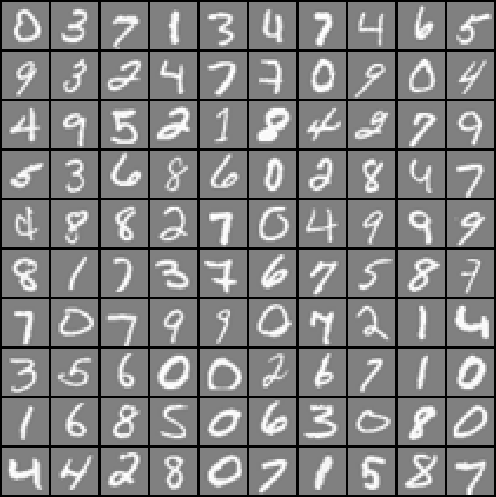
Figure 1: Random samples selected from the MNIST dataset

Zero-sum attacks: As depicted in Fig. (2a), an $m=30$ multi-agent CPS consists of ${\left|\mathcal{R}\right|}=25$ reliable agents (yellow nodes) and $\left|\mathcal{B}\right|=5$ Byzantine agents (red nodes), where each Byzantine agent $o$, $o\in\mathcal{B}$, sends a well-designed malicious message ${z_{io,k}}=-{\sum\nolimits_{j\in{\mathcal{R}_{i}}}{{w_{ij}}{x_{j,k}}}}/\left|{{\mathcal{B}_{i}}}\right|/{w_{oi}}$ to its reliable neighbor $i$, $i\in{\mathcal{R}_{o}}$, to let the states of the reliable agent ${x_{i,k}}=0_{n}$ at each iteration. For NIDS [37], we choose the algorithm parameter $c=1/\left({2{{\max}_{i\in\mathcal{R}}}\left\{{{\alpha_{i}}}\right\}}\right)$ for $\tilde{W}={I_{m}}-c{D_{\alpha}}\left({{I_{m}}-W}\right)$, where $\tilde{W}$, $W$, and $D_{\alpha}$ are the modified mixing matrix, weight matrix, and uncoordinated step-size, respectively. This means if $c$ is sufficiently small, NIDS runs without any communication happening among all agents (both reliable agents and Byzantine agents) over networks. For PMGT-SAGA/PMGT-LSVRG [35], we hand-tune the parameter associated with multi-step communications to obtain the best performance. It is clear from Figs. (2b)-(2d) and Table II that both Prox-DBRO-SAGA and Prox-DBRO-LSVRG achieve a smaller optimality gap and higher testing accuracy than the other tested algorithms in a same amount of computational costs (epochs). This demonstrates that Prox-DBRO-SAGA and Prox-DBRO-LSVRG approximate faster to the optimal solution than the other tested algorithms. It is worthwhile to mention that zero-sum attacks launched by Byzantine agents aim to drive the states of all reliable agents to zero in each iteration. Therefore, the much smaller consensus error of NIDS and PMGT-SAGA/PMGT-LSVRG than the other decentralized Byzantine-resilient algorithms, indicates reversely that they are vulnerable to the zero-sum attacks. Likewise, the bigger consensus error of Prox-DBRO-SAGA and Prox-DBRO-LSVRG means that they are more robust to the zero-sum attacks than the other tested algorithms.

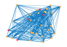
(a) A 30-agent network containing $5$ Byzantine agents.

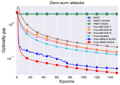
(b) Optimality gaps over epochs.

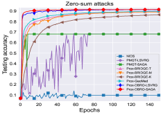
(c) Testing accuracy over epochs.

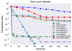
(d) Consensus errors over epochs.

Figure 2: Performance of all tested algorithms over a Byzantine network under zero-sum attacks.

	NIDS	PMGT-LSVRG	PMGT-SAGA	Prox-BRIDGE-T	Prox-BRIDGE-M	Prox-BRIDGE-K	Prox-GeoMed	Prox-DBRO-LSVRG	Prox-DBRO-SAGA
Step-Size	[0.01, 0.015]	0.001	0.01	0.35	0.3	0.35	0.35	0.05	0.005
Triggered Probability	N/A	$m/Q$	N/A	N/A	N/A	N/A	N/A	$\left[{m/Q/2,m/Q}\right]$	N/A
Penalty Parameter	N/A	N/A	N/A	N/A	N/A	N/A	N/A	[0.2, 0.25]	[0.2, 0.25]
Consensus Error	0	1.2650e-06	1.2621e-06	0.0012	0.0019	0.0019	0.0010	4.4680	0.0428
Testing Accuracy	0.098	0.6843	0.6846	0.8967	0.8918	0.8653	0.8992	0.9137	0.9155
Optimality Gap	2.0245	1.9230	1.9228	1.4710e-01	1.5514e-01	2.1553e-01	1.2826e-01	5.0790e-02	3.7756e-02
S&PI is the abbreviation of settings and performance indices.

TABLE II: Parameter settings and algorithm performance at 150 epochs under zero-sum attacks.

Gaussian attacks: It is shown in Fig. (3a) that an $m=40$ multi-agent CPS consists of ${\left|\mathcal{R}\right|}=32$ reliable agents (yellow nodes) and $\left|\mathcal{B}\right|=8$ Byzantine agents (red nodes), where each Byzantine agent $o$, $o\in\mathcal{B}$, sends a message generated by a Gaussian distribution with mean $\sum\nolimits_{j\in{\mathcal{R}_{i}}}{{w_{ij}}{x_{j,k}}}/\sum\nolimits_{j\in{\mathcal{R}_{i}}}{{w_{ij}}}$ and standard deviation 30, to its reliable neighbor $i$, $i\in{\mathcal{R}_{o}}$ at each iteration. This attack serves as a Gaussian noise, which can easily inflict fluctuation on the status of reliable agents and deviate the states from their true values. Even though the testing accuracy index can still fluctuate around 0.6, we can see from Fig. (3b) and Table III that NIDS and PMGT-SAGA/PMGT-LSVRG show divergence from the optimal solution under Gaussian attacks. This is the gap between theoretical results and experimental performance. It is shown by Figs. (3b)-(3d) that Prox-DBRO-SAGA and Prox-DBRO-LSVRG can still achieve a smaller optimality gap and higher testing accuracy in the same epochs, alternatively faster convergence, than the other tested algorithms. Moreover, one can clearly see from Table III that Prox-DBRO-SAGA takes the superiority on all three performance indices (consensus errors, testing accuracy, and optimality gaps) at 150 epochs, while Prox-DBRO-LSVRG ranks the second leading position on these three performance indices.

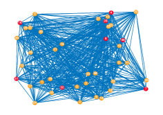
(a) A 40-agent network containing $8$ Byzantine agents.

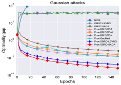
(b) Optimality gaps over epochs.

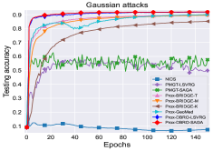
(c) Testing accuracy over epochs.

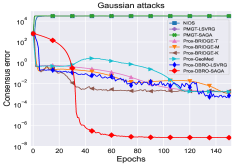
(d) Consensus errors over epochs.

Figure 3: Performance of all tested algorithms under Gaussian attacks.

	NIDS	PMGT-LSVRG	PMGT-SAGA	Prox-BRIDGE-T	Prox-BRIDGE-M	Prox-BRIDGE-K	Prox-GeoMed	Prox-DBRO-LSVRG	Prox-DBRO-SAGA
Step-Size	[0.3, 0.35]	0.3	0.3	0.4	0.3	0.3	0.4	0.02	0.0025
Triggered Probability	N/A	$m/Q$	N/A	N/A	N/A	N/A	N/A	$\left[{m/Q/4,m/Q/2}\right]$	N/A
Penalty Parameter	N/A	N/A	N/A	N/A	N/A	N/A	N/A	[0.05, 0.055]	[0.005, 0.0055]
Consensus Error	7.7540e+04	3.2041e+04	3.1770e+04	1.7037e-03	1.1220e-03	1.9835e-03	0.9002	0.0007	6.71366e-08
Testing Accuracy	8.1060e-01	4.9850e-01	5.7650e-01	8.9920e-01	8.9540e-01	8.5220e-01	0.0017	0.9182	9.1970
Optimality Gap	Inf	3.9609e+01	3.1770e+04	1.2136e-01	1.4870e-01	2.4074e-01	1.1507e-01	4.0442e-02	2.4398e-02
S&PI is the abbreviation of settings and performance indices.

TABLE III: Parameter settings and algorithm performance at 150 epochs under Gaussian attacks.

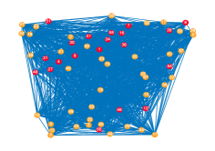
(a) A 60-agent network containing $20$ Byzantine agents.

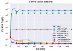
(b) Optimality gaps over epochs.

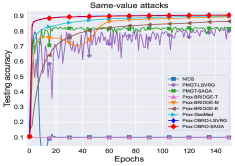
(c) Testing accuracy over epochs.

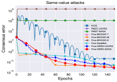
(d) Consensus errors over epochs.

Figure 4: Performance of all tested algorithms under same-value attacks.

	NIDS	PMGT-LSVRG	PMGT-SAGA	Prox-BRIDGE-T	Prox-BRIDGE-M	Prox-BRIDGE-K	Prox-GeoMed	Prox-DBRO-LSVRG	Prox-DBRO-SAGA
Step-Size	[0.5, 0.55]	0.5	0.5	0.2	0.3	0.4	0.4	$0.35/\sqrt{k+1}$	$0.11/\sqrt{k+1}$
Triggered Probability	N/A	$m/Q$	N/A	N/A	N/A	N/A	N/A	$\left[{m/Q/8,m/Q/4}\right]$	N/A
Penalty Parameter	N/A	N/A	N/A	N/A	N/A	N/A	N/A	[0.0005, 0.00055]	[0.0005, 0.00055]
Consensus Error	0.0417	1121561.6743	1121561.6458	0.0514	0.00174	190905836.8303	0.0027	0.0006	0.0008
Testing Accuracy	0.098	0.8019	0.8162	0.8023	0.8942	0.8649	0.9006	0.9065	0.9055
Optimality Gap	6.5336e+04	2.2774e+04	2.2774e+04	Inf	1.7867e-01	4.2663e+01	1.6547e-01	1.6316e-01	1.6534e-01
S&PI is the abbreviation of settings and performance indices.

TABLE IV: Parameter settings and algorithm performance at 150 epochs under same-value attacks.

Same-value attacks: As depicted in (4a), an $m=60$ multi-agent CPS consists of ${\left|\mathcal{R}\right|}=40$ reliable agents (yellow nodes) and $\left|\mathcal{B}\right|=20$ Byzantine agents (red nodes), where each Byzantine agent $o$, $o\in\mathcal{B}$, keeps sending ${z_{io,k}}=1000*{1_{n}}$ to its reliable neighbor $i$, $i\in{\mathcal{R}_{o}}$, at each iteration. Under this attack, the states of reliable agents can be easily blown up to sufficiently large values, which prevents the tested algorithms from convergence. Figs. (4b)-(4c) manifest that both Prox-DBRO-SAGA and Prox-DBRO-LSVRG achieve faster convergence than the other tested algorithms on the performance indices of OG and testing accuracy, while Prox-DBRO-LSVRG is slightly faster than Prox-DBRO-SAGA in this case. It can be found in Table IV that both Prox-DBRO-SAGA and Prox-DBRO-LSVRG attain also a smaller consensus error than the other tested algorithms at the final epoch. Note that the performance comparison takes no account of BRIDGE-B [23] due to its strict requirement of the number of its neighboring agents and high computational overhead. In a nutshell, the above simulation results demonstrate that Prox-DBRO-LSVRG and Prox-DBRO-SAGA achieve better convergence performance under different kinds of Byzantine attacks.

VI Conclusions

In this paper, we proposed two decentralized Byzantine-resilient and variance-reduced stochastic gradient algorithms, namely Prox-DBRO-LSVRG and Prox-DBRO-SAGA, to resolve a category of non-smooth composite optimization problems over multi-agent CPSs in the presence of Byzantine agents. Theoretical analysis established both linear and sub-linear convergence rates for Prox-DBRO-LSVRG and Prox-DBRO-SAGA under different assumptions and parameter selections. In simulation, the proposed algorithms were applied to resolving a decentralized sparse soft-max regression task over multi-agent CPSs under different Byzantine attacks, which verifies the theoretical findings and demonstrates the better convergence performance of Prox-DBRO-LSVRG and Prox-DBRO-SAGA than the other notable decentralized algorithms. Future work will focus on extending the theoretical analysis of Prox-DBRO-LSVRG and Prox-DBRO-SAGA to the more general non-convex domain.

-A Proof of Lemma 1

According to Step 4 in Algorithm 3, at iteration $k$, $\forall k\geq 1$, the auxiliary variables $u_{i,k+1}^{l}$, $i\in\mathcal{R}$, take value $u_{i,k}^{l}$ or ${x_{i,k}}$, associated with probabilities $1-1/q_{i}$ and $1/q_{i}$, respectively. This observation is owing to the fact that selection of the random sample for Prox-DBRO-SAGA, at each iteration $k\geq 1$, is uniformly and independently executed. Hence, we have

$${\mathbb{E}_{k}}\left[{\frac{1}{{{q_{i}}}}\sum\limits_{l=1}^{{q_{i}}}{{\nabla f_{i}^{l}{{\left({{{\tilde{x}}^{*}}}\right)}^{\top}}\left({u_{i,k+1}^{l}-{{\tilde{x}}^{*}}}\right)}}}\right]$$ (15)

$$= \left({1-\frac{1}{{{q_{i}}}}}\right)\frac{1}{{{q_{i}}}}\sum\limits_{l=1}^{{q_{i}}}{\nabla f_{i}^{l}{{\left({{{\tilde{x}}^{*}}}\right)}^{\top}}\left({u_{i,k}^{l}-{{\tilde{x}}^{*}}}\right)}+\frac{1}{{{q_{i}}}}\nabla{f_{i}}{\left({{{\tilde{x}}^{*}}}\right)^{\top}}$$

$$\times\left({{x_{i,k}}-{{\tilde{x}}^{*}}}\right).$$

Similarly, it holds that

$${\mathbb{E}_{k}}\left[{f_{i}^{l}\left({u_{i,k+1}^{l}}\right)}\right]=\left({1-\frac{1}{{{q_{i}}}}}\right)f_{i}^{l}\left({u_{i,k}^{l}}\right)+\frac{1}{{{q_{i}}}}f_{i}^{l}\left({{x_{i,k}}}\right).$$ (16)

Via summing (16) over index $l$ for all $l=1,\ldots,{q_{i}}$, we can further obtain

$${\mathbb{E}_{k}}\left[{\frac{1}{{{q_{i}}}}\sum\limits_{l=1}^{{q_{i}}}{f_{i}^{l}\left({u_{i,k+1}^{l}}\right)}}\right]$$ (17)

$$= \left({1-\frac{1}{{{q_{i}}}}}\right)\frac{1}{{{q_{i}}}}\sum\limits_{l=1}^{{q_{i}}}{f_{i}^{l}\left({u_{i,k}^{l}}\right)}+\frac{1}{{{q_{i}}}}\frac{1}{{{q_{i}}}}\sum\limits_{l=1}^{{q_{i}}}{f_{i}^{l}\left({{x_{i,k}}}\right)}$$

$$= \left({1-\frac{1}{{{q_{i}}}}}\right)\frac{1}{{{q_{i}}}}\sum\limits_{l=1}^{{q_{i}}}{f_{i}^{l}\left({u_{i,k}^{l}}\right)}+\frac{1}{{{q_{i}}}}{f_{i}}\left({{x_{i,k}}}\right).$$

Recalling the definition of $t_{i,k}^{u}$ and combining Eqs. (15) and (17) give

$${\mathbb{E}_{k}}\left[{t_{i,k+1}^{u}}\right]$$ (18)

$$= {\mathbb{E}_{k}}\!\!\left[{\frac{1}{{{q_{i}}}}\sum\limits_{l=1}^{{q_{i}}}{f_{i}^{l}\left({u_{i,k+1}^{l}}\right)}\!-\!{f_{i}}\left({{{\tilde{x}}^{*}}}\right)\!-\!\nabla f_{i}^{l}{{\left({{{\tilde{x}}^{*}}}\right)}^{\top}}\left({u_{i,k+1}^{l}\!-{{\tilde{x}}^{*}}}\right)}\right]$$

$$= \left({1-\frac{1}{{{q_{i}}}}}\right)\frac{1}{{{q_{i}}}}\sum\limits_{l=1}^{{q_{i}}}{f_{i}^{l}\left({u_{i,k}^{l}}\right)-\nabla f_{i}^{l}{{\left({{{\tilde{x}}^{*}}}\right)}^{\top}}\left({u_{i,k}^{l}-{{\tilde{x}}^{*}}}\right)}$$

$$+\frac{1}{{{q_{i}}}}{f_{i}}\left({{x_{i,k}}}\right)-{f_{i}}\left({{{\tilde{x}}^{*}}}\right)-\frac{1}{{{q_{i}}}}\nabla{f_{i}}{\left({{{\tilde{x}}^{*}}}\right)^{\top}}\left({{x_{i,k}}-{{\tilde{x}}^{*}}}\right)$$

$$= \left({1-\frac{1}{{{q_{i}}}}}\right){t_{i,k}}+\frac{1}{{{q_{i}}}}\left({{f_{i}}\left({{x_{i,k}}}\right)-{f_{i}}\left({{{\tilde{x}}^{*}}}\right)}\right)-\frac{1}{{{q_{i}}}}\nabla{f_{i}}{\left({{{\tilde{x}}^{*}}}\right)^{\top}}$$

$$\times\left({{x_{i,k}}-{{\tilde{x}}^{*}}}\right).$$

Summing Eq. (18) over $i$ yields

$$\sum\limits_{i\in\mathcal{R}}{{\mathbb{E}_{k}}\left[{t_{i,k+1}^{u}}\right]}$$ (19)

$$= \sum\limits_{i\in\mathcal{R}}{\frac{1}{{{q_{i}}}}\left({{f_{i}}\left({{x_{i,k}}}\right)-{f_{i}}\left({{{\tilde{x}}^{*}}}\right)-\nabla{f_{i}}{{\left({{{\tilde{x}}^{*}}}\right)}^{\top}}\left({{x_{i,k}}-{{\tilde{x}}^{*}}}\right)}\right)}$$

$$+\sum\limits_{i\in\mathcal{R}}{\left({1-\frac{1}{{{q_{i}}}}}\right)t_{i,k}^{u}}$$

$$\leq \frac{1}{{{q_{\min}}}}\sum\limits_{i\in\mathcal{R}}{{{f_{i}}\left({{x_{i,k}}}\right)-{f_{i}}\left({{{\tilde{x}}^{*}}}\right)-\nabla{f_{i}}{{\left({{{\tilde{x}}^{*}}}\right)}^{\top}}\left({{x_{i,k}}-{{\tilde{x}}^{*}}}\right)}}$$

$$+\left({1-\frac{1}{{{q_{\max}}}}}\right)\sum\limits_{i\in\mathcal{R}}{t_{i,k}^{u}}$$

$$= \frac{1}{{{q_{\min}}}}{D_{F}}\left({{x_{k}},{x^{*}}}\right)+\left({1-\frac{1}{{{q_{\max}}}}}\right)\sum\limits_{i\in\mathcal{R}}{t_{i,k}^{u}},$$

where the second inequality uses $1\leq{q_{\min}}\leq{q_{i}}\leq{q_{\max}}$, and the last equality is according to $f\left(x\right)=\sum\nolimits_{i\in\mathcal{R}}{{f_{i}}\left({{x_{i}}}\right)}$ and the definition of ${D_{F}}\left({{x_{k}},{x^{*}}}\right)$. Substituting the definition of $t_{k}^{u}$ obtains the relation (8). In view of Step 4 in Algorithm 2, we know that at iteration $k$, $\forall k\geq 1$, the auxiliary variables ${w_{i,k+1}}$, $i\in\mathcal{R}$, take value ${x_{i,k}}$ with probability $p_{i}$, or keep the most recent update ${w_{i,k}}$ with probability $1-{p_{i}}$. Therefore, it can be verified that

$${\mathbb{E}_{k}}\left[{\frac{1}{{{q_{i}}}}\sum\limits_{l=1}^{{q_{i}}}{{\nabla f_{i}^{l}{{\left({{{\tilde{x}}^{*}}}\right)}^{\top}}\left({{w_{i,k+1}}-{{\tilde{x}}^{*}}}\right)}}}\right]$$ (20)

$$= \frac{{{p_{i}}}}{{{q_{i}}}}\sum\limits_{l=1}^{{q_{i}}}{\nabla f_{i}^{l}{{\left({{{\tilde{x}}^{*}}}\right)}^{\top}}\left({{x_{i,k}}\!-\!{{\tilde{x}}^{*}}}\right)}\!+\!\left({1\!-\!{p_{i}}}\right)\nabla{f_{i}}{\left({{{\tilde{x}}^{*}}}\right)^{\top}}({{w_{i,k}}\!-\!{{\tilde{x}}^{*}}}).$$

Likewise, we have

$${\mathbb{E}_{k}}\!\!\left[{\frac{1}{{{q_{i}}}}\sum\limits_{l=1}^{{q_{i}}}{f_{i}^{l}\left({{w_{i,k+1}}}\right)}}\right]\\ \!\!\!=\!\left({1\!-\!{p_{i}}}\right)\frac{1}{{{q_{i}}}}\sum\limits_{l=1}^{{q_{i}}}{f_{i}^{l}\left({{w_{i,k}}}\right)}+{p_{i}}{f_{i}}\left({{x_{i,k}}}\right).$$ (21)

Recalling the definition of $t_{i,k}^{w}$ and combining Eq. (20) with (21) give

$${\mathbb{E}_{k}}\left[{t_{i,k+1}^{w}}\right]$$ (22)

$$= {\mathbb{E}_{k}}\left[{\frac{1}{{{q_{i}}}}\sum\limits_{l=1}^{{q_{i}}}{f_{i}^{l}\left({{w_{i,k+1}}}\right)}\!-\!{f_{i}}\left({{{\tilde{x}}^{*}}}\right)\!-\!\nabla f_{i}^{l}{{\left({{{\tilde{x}}^{*}}}\right)}^{\top}}\left({{w_{i,k+1}}\!-\!{{\tilde{x}}^{*}}}\right)}\right]$$

$$= \left({1\!-{p_{i}}}\right){t_{i,k}^{w}}\!+\!{p_{i}}({{f_{i}}\left({{x_{i,k}}}\right)\!-\!{f_{i}}\left({{{\tilde{x}}^{*}}}\right)\!-\!\nabla{f_{i}}{{\left({{{\tilde{x}}^{*}}}\right)}^{\top}}\left({{x_{i,k}}\!-\!{{\tilde{x}}^{*}}}\right)}),$$

where we apply ${f_{i}}\left({{{\tilde{x}}^{*}}}\right)=\left({1/{q_{i}}}\right)\sum\nolimits_{l=1}^{{q_{i}}}{f_{i}^{l}\left({{\tilde{x}}^{*}}\right)}$ in the last equality. The relation (9) is reached through summing Eq. (22) over $i$ and substituting the definitions of $t_{k}^{w}$ and ${D_{F}}\left({{x_{k}},{x^{*}}}\right)$.

-B Proof of Lemma 2

According to Step 3 in Algorithm 2, it holds that

$${\mathbb{E}_{k}}\left[{\left\|{r_{i,k}^{u}-\nabla{f_{i}}\left({{{\tilde{x}}^{*}}}\right)}\right\|_{2}^{2}}\right]$$ (23)

$$= {\mathbb{E}_{k}}\left[{\left\|{r_{i,k}^{u}-\nabla{f_{i}}\left({{{\tilde{x}}^{*}}}\right)-\nabla{f_{i}}\left({{x_{i,k}}}\right)+\nabla{f_{i}}\left({{{\tilde{x}}^{*}}}\right)}\right\|_{2}^{2}}\right]$$

$$+\left\|{\nabla{f_{i}}\left({{x_{i,k}}}\right)-\nabla{f_{i}}\left({{{\tilde{x}}^{*}}}\right)}\right\|_{2}^{2},$$

where the equality is due to the standard variance decomposition $\mathbb{E}_{k}\left[{\left\|A\right\|_{2}^{2}}\right]=\left\|{\mathbb{E}_{k}\left[A\right]}\right\|_{2}^{2}+\mathbb{E}_{k}\left[{\left\|{A-\mathbb{E}_{k}\left[A\right]}\right\|_{2}^{2}}\right]$, with $A={r_{i,k}^{u}}-\nabla{f_{i}}\left({{{\tilde{x}}^{*}}}\right)$. We continue to handle the first term in the right-hand-side of Eq. (23) as follows:

$${\mathbb{E}_{k}}\left[{\left\|{r_{i,k}^{u}-\nabla{f_{i}}\left({{{\tilde{x}}^{*}}}\right)-\nabla{f_{i}}\left({{x_{i,k}}}\right)+\nabla{f_{i}}\left({{{\tilde{x}}^{*}}}\right)}\right\|_{2}^{2}}\right]$$ (24)

$$\leq 2{\mathbb{E}_{k}}\!\!\left[{\left\|{\nabla f_{i}^{{s_{i,k}}}\!\left({{x_{i,k}}}\right)\!-\!\nabla f_{i}^{{s_{i,k}}}\left({{{\tilde{x}}^{*}}}\right)\!-\!\nabla{f_{i}}\left({{x_{i,k}}}\right)\!+\!\nabla{f_{i}}\left({{{\tilde{x}}^{*}}}\right)}\right\|_{2}^{2}}\right]$$

$$+2{\mathbb{E}_{k}}\!\left[{\left\|{\nabla f_{i}^{{s_{i,k}}}\left({u_{i,k}^{{s_{i,k}}}}\right)-\nabla f_{i}^{{s_{i,k}}}\left({{{\tilde{x}}^{*}}}\right)-\frac{1}{{{q_{i}}}}\sum\limits_{l=1}^{{q_{i}}}{\nabla f_{i}^{l}\left({u_{i,k}^{l}}\right)}}\right.}\right.$$

$$+\left.{\left.{\nabla{f_{i}}\left({{{\tilde{x}}^{*}}}\right)}\right\|_{2}^{2}}\right]$$

$$\leq 2{\mathbb{E}_{k}}\!\!\left[{\left\|{\nabla f_{i}^{{s_{i,k}}}\left({{x_{i,k}}}\right)\!-\!\nabla f_{i}^{{s_{i,k}}}\left({{{\tilde{x}}^{*}}}\right)\!-\!\nabla{f_{i}}\left({{x_{i,k}}}\right)\!+\!\nabla{f_{i}}\left({{{\tilde{x}}^{*}}}\right)}\right\|_{2}^{2}}\right]$$

$$+2{\mathbb{E}_{k}}\left[{\left\|{\nabla f_{i}^{{s_{i,k}}}\left({u_{i,k}^{{s_{i,k}}}}\right)-\nabla f_{i}^{{s_{i,k}}}\left({{{\tilde{x}}^{*}}}\right)}\right\|_{2}^{2}}\right]$$

$$= 2{\mathbb{E}_{k}}\left[{\left\|{\nabla f_{i}^{{s_{i,k}}}\left({{x_{i,k}}}\right)-\nabla f_{i}^{{s_{i,k}}}\left({{{\tilde{x}}^{*}}}\right)}\right\|_{2}^{2}}\right]$$

$$+2{\mathbb{E}_{k}}\left[{\left\|{\nabla f_{i}^{{s_{i,k}}}\left({u_{i,k}^{{s_{i,k}}}}\right)-\nabla f_{i}^{{s_{i,k}}}\left({{{\tilde{x}}^{*}}}\right)}\right\|_{2}^{2}}\right]$$

$$-2\left\|{\nabla{f_{i}}\left({{x_{i,k}}}\right)-\nabla{f_{i}}\left({{{\tilde{x}}^{*}}}\right)}\right\|_{2}^{2},$$

where the second inequality utilizes $\mathbb{E}_{k}\left[{\left\|{B-\mathbb{E}_{k}\left[B\right]}\right\|_{2}^{2}}\right]\leq\mathbb{E}_{k}\left[{\left\|B\right\|_{2}^{2}}\right]$, with $B=\nabla f_{i}^{{s_{i,k}}}\left({u_{i,k}^{{s_{i,k}}}}\right)-\nabla f_{i}^{{s_{i,k}}}\left({{{\tilde{x}}^{*}}}\right)$, and the last equality applies the standard variance decomposition again. We proceed with substituting (24) into (23) to obtain

$${\mathbb{E}_{k}}\left[{\left\|{r_{i,k}^{u}-\nabla{f_{i}}\left({{{\tilde{x}}^{*}}}\right)}\right\|_{2}^{2}}\right]$$ (25)

$$= 2{\mathbb{E}_{k}}\left[{\left\|{\nabla f_{i}^{{s_{i,k}}}\left({{x_{i,k}}}\right)-\nabla f_{i}^{{s_{i,k}}}\left({{{\tilde{x}}^{*}}}\right)}\right\|_{2}^{2}}\right]$$

$$+2{\mathbb{E}_{k}}\left[{\left\|{\nabla f_{i}^{{s_{i,k}}}\left({u_{i,k}^{{s_{i,k}}}}\right)-\nabla f_{i}^{{s_{i,k}}}\left({{{\tilde{x}}^{*}}}\right)}\right\|_{2}^{2}}\right]$$

$$-\left\|{\nabla{f_{i}}\left({{x_{i,k}}}\right)-\nabla{f_{i}}\left({{{\tilde{x}}^{*}}}\right)}\right\|_{2}^{2}.$$

Summing Eq. (25) over $i$ generates

$${\mathbb{E}_{k}}\left[{\left\|{r_{k}^{u}-\nabla f\left({{{\tilde{x}}^{*}}}\right)}\right\|_{2}^{2}}\right]$$ (26)

$$\leq 2\sum\limits_{i\in\mathcal{R}}{{\mathbb{E}_{k}}\left[{\left\|{\nabla f_{i}^{{s_{i,k}}}\left({{x_{i,k}}}\right)-\nabla f_{i}^{{s_{i,k}}}\left({{{\tilde{x}}^{*}}}\right)}\right\|_{2}^{2}}\right]}$$

$$+2\sum\limits_{i\in\mathcal{R}}{{\mathbb{E}_{k}}\left[{\left\|{\nabla f_{i}^{{s_{i,k}}}\left({u_{i,k}^{{s_{i,k}}}}\right)-\nabla f_{i}^{{s_{i,k}}}\left({{{\tilde{x}}^{*}}}\right)}\right\|_{2}^{2}}\right]}$$

$$-\sum\limits_{i\in\mathcal{R}}{\left\|{\nabla{f_{i}}\left({{x_{i,k}}}\right)-\nabla{f_{i}}\left({{{\tilde{x}}^{*}}}\right)}\right\|_{2}^{2}}.$$

Since the local component objective function $f_{i}^{l}$, $\forall l\in\mathcal{Q}_{i}$ and $\forall i\in\mathcal{R}$, is $L$-smooth according to Assumption 1, we have

$$\frac{1}{{2L}}\left\|{\nabla f_{i}^{l}\left({u_{i,k}^{l}}\right)-\nabla{f_{i,l}}\left({{{\tilde{x}}^{*}}}\right)}\right\|_{2}^{2}$$ (27)

$$\leq f_{i}^{l}\left({u_{i,k}^{l}}\right)-f_{i}^{l}\left({{{\tilde{x}}^{*}}}\right)-\nabla f_{i}^{l}{\left({{{\tilde{x}}^{*}}}\right)^{\top}}\left({u_{i,k}^{l}-{{\tilde{x}}^{*}}}\right).$$

Summing the both sides of (27) over $l$ from $1$ to $q_{i}$ becomes

$$\frac{1}{{{q_{i}}}}\sum\limits_{l=1}^{{q_{i}}}{\left\|{\nabla f_{i}^{l}\left({u_{i,k}^{l}}\right)-\nabla f_{i}^{l}\left({{{\tilde{x}}^{*}}}\right)}\right\|_{2}^{2}}\leq 2Lt_{i,k}^{u}.$$ (28)

Since the local component function $f_{i}^{{s_{i,k}}}$, has a uniform distribution over the set $\left\{{f_{i}^{1},\ldots,f_{i}^{{q_{i}}}}\right\}$, it is natural to obtain

$${\mathbb{E}_{k}}\left[{\left\|{\nabla f_{i}^{{s_{i,k}}}\left({u_{i,k}^{{s_{i,k}}}}\right)-\nabla f_{i}^{{s_{i,k}}}\left({{{\tilde{x}}^{*}}}\right)}\right\|_{2}^{2}}\right]$$ (29)

$$= \frac{1}{{{q_{i}}}}\sum\limits_{l=1}^{{q_{i}}}{\left\|{\nabla f_{i}^{l}\left({u_{i,k}^{l}}\right)-\nabla f_{i}^{l}\left({{{\tilde{x}}^{*}}}\right)}\right\|_{2}^{2}}.$$

Combining Eq. (29) and (28) and then summing over $i$ yield

$$\sum\limits_{i\in\mathcal{R}}{{\mathbb{E}_{k}}\left[{\left\|{\nabla f_{i}^{{s_{i,k}}}\left({u_{i,k}^{{s_{i,k}}}}\right)-\nabla f_{i}^{{s_{i,k}}}\left({{{\tilde{x}}^{*}}}\right)}\right\|_{2}^{2}}\right]}\leq 2Lt_{k}^{u}.$$ (30)

Summarizing (26) and (30) obtains

$${\mathbb{E}_{k}}\left[{\left\|{r_{k}^{u}-\nabla f\left({{{\tilde{x}}^{*}}}\right)}\right\|_{2}^{2}}\right]$$ (31)

$$\leq 4Lt_{k}^{u}+2\sum\limits_{i\in\mathcal{R}}{{\mathbb{E}_{k}}\left[{\left\|{\nabla f_{i}^{{s_{i,k}}}\left({{x_{i,k}}}\right)-\nabla f_{i}^{{s_{i,k}}}\left({{{\tilde{x}}^{*}}}\right)}\right\|_{2}^{2}}\right]}$$

$$-\left\|{\nabla F\left({{x_{k}}}\right)-\nabla F\left({{x^{*}}}\right)}\right\|_{2}^{2},$$

where we simplify $\sum\nolimits_{i\in\mathcal{R}}{\left\|{\nabla{f_{i}}\left({{x_{i,k}}}\right)-\nabla{f_{i}}\left({{{\tilde{x}}^{*}}}\right)}\right\|_{2}^{2}}$ as $\left\|{\nabla F\left({{x_{k}}}\right)-\nabla F\left({{x^{*}}}\right)}\right\|_{2}^{2}$. Via applying the Lipschitz continuity of $\nabla f_{i}^{l}$ again, we have

$$\sum\limits_{i\in\mathcal{R}}{{\mathbb{E}_{k}}\left[{\left\|{\nabla f_{i}^{{s_{i,k}}}\left({{x_{i,k}}}\right)-\nabla f_{i}^{{s_{i,k}}}\left({{{\tilde{x}}^{*}}}\right)}\right\|_{2}^{2}}\right]}\leq 2L{D_{F}}\left({{x_{k}},{x^{*}}}\right),$$ (32)

where we use the fact that ${f_{i}}\left({{x_{i,k}}}\right)=\left({1/{q_{i}}}\right)\sum\nolimits_{l=1}^{{q_{i}}}{f_{i}^{l}\left({{x_{i,k}}}\right)}$ and $f\left(x_{k}\right)=\sum\nolimits_{i\in\mathcal{R}}{{f_{i}}\left({{x_{i,k}}}\right)}$. Plugging (32) into (31) generates

$${\mathbb{E}_{k}}\left[{\left\|{r_{k}^{u}-\nabla f\left({{{\tilde{x}}^{*}}}\right)}\right\|_{2}^{2}}\right]$$ (33)

$$\leq 4Lt_{k}^{u}+4L{D_{F}}\left({{x_{k}},{x^{*}}}\right)-\left\|{\nabla F\left({{x_{k}}}\right)-\nabla F\left({{x^{*}}}\right)}\right\|_{2}^{2}.$$

Considering the $\mu$-strong convexity of the local objective function $f_{i}$, $\forall i\in\mathcal{R}$, we have

$$2\mu{D_{F}}\left({{x_{k}},{x^{*}}}\right)\leq\left\|{\nabla F\left({{x_{k}}}\right)-\nabla F\left({{x^{*}}}\right)}\right\|_{2}^{2}.$$ (34)

Finally, one can obtain (10) via plugging the relation (34) into (33). For Prox-DBRO-LSVRG, we replace ${u_{i,k}^{l}}$ with ${{w_{i,k}}}$ to obtain (11), which completes the proof.

-C Proof of Proposition 2

According to the definition of ${\mathbf{prox}}_{\alpha,G}\left\{x\right\}$, we have

$${\mathbf{prox}}_{\alpha,G}\left\{x\right\}$$ (35)

$$= \arg\mathop{\min}\limits_{y}\left\{{G\left(y\right)+\frac{1}{{2\alpha}}\left\|{y-x}\right\|_{2}^{2}}\right\}$$

$$= \arg\mathop{\min}\limits_{y}\left\{{\sum\limits_{i\in\mathcal{R}}{g\left({{y_{i}}}\right)}+\frac{1}{{2\alpha}}\sum\limits_{i\in\mathcal{R}}{\left\|{{y_{i}}-{x_{i}}}\right\|_{2}^{2}}}\right\}$$

$$= \left({\begin{array}[]{*{20}{c}}{\arg\mathop{\min}\limits_{\tilde{y}\in{\mathbb{R}^{n}}}\left\{{g\left({\tilde{y}}\right)+\frac{1}{{2\alpha}}\left\|{\tilde{y}-{x_{1}}}\right\|_{2}^{2}}\right\}}\\ {\arg\mathop{\min}\limits_{\tilde{y}\in{\mathbb{R}^{n}}}\left\{{g\left({\tilde{y}}\right)+\frac{1}{{2\alpha}}\left\|{\tilde{y}-{x_{2}}}\right\|_{2}^{2}}\right\}}\\ \vdots\\ {\arg\mathop{\min}\limits_{\tilde{y}\in{\mathbb{R}^{n}}}\left\{{g\left({\tilde{y}}\right)+\frac{1}{{2\alpha}}\left\|{\tilde{y}-{x_{\left|\mathcal{R}\right|}}}\right\|_{2}^{2}}\right\}}\end{array}}\right),$$

which indicates ${\left[{\mathbf{prox}}_{\alpha,G}\left\{x\right\}\right]}_{i}={\mathbf{prox}}_{\alpha,g}\left\{x_{i}\right\}$. Based on this equality, it is straightforward to verify (12) with the help of the non-expansiveness of the proximal operator ${{\mathbf{prox}}_{\alpha,g}}$, which completes the proof.

-D Proof of Theorem 1

The optimal solution to (4) satisfies the optimality condition

$${0_{n}}\in{\nabla{f_{i}}\left({x_{i}^{*}}\right)+\partial_{x_{i}}g\left({x_{i}^{*}}\right)}+\frac{{{\phi_{i}}}}{2}\sum\limits_{j\in{\mathcal{R}_{i}}}{\partial{{\left\|{x_{i}^{*}-x_{j}^{*}}\right\|}_{a}}},\forall i\in\mathcal{R}.$$ (36)

According to the definition of the sub-differential ${\partial}{\left\|{x_{i}^{*}-x_{j}^{*}}\right\|_{a}}=\left\{{{y_{ij}}\in{\mathbb{R}^{n}}|\left\langle{{y_{ij}},x_{i}^{*}}\right\rangle={{\left\|{x_{i}^{*}}\right\|}_{a}},{{\left\|{{y_{ij}}}\right\|}_{b}}\leq 1}\right\}$, there exist $g_{x_{i}}^{*}\in\partial_{x_{i}}g\left({x_{i}^{*}}\right)$ and ${\tilde{y}_{ij}}\in{\partial}{\left\|{x_{i}^{*}-x_{j}^{*}}\right\|_{a}}$, such that for $\forall i\in\mathcal{R}$

$${\nabla{f_{i}}\left({x_{i}^{*}}\right)+g_{x_{i}}^{*}}+{\phi_{i}}\left({\sum\limits_{j\in{\mathcal{R}_{i}},i<j}{{{\tilde{y}}_{ij}}}-\sum\limits_{j\in{\mathcal{R}_{i}},i>j}{{{\tilde{y}}_{ji}}}}\right)=0_{n}.$$ (37)

Under Assumption 1, the globally optimal solution $x^{*}$ exists uniquely. We next need to prove that the optimal solution ${\tilde{x}^{*}}$ satisfies (37), such that

$${\nabla{f_{i}}\left({{{\tilde{x}}^{*}}}\right)+g_{\tilde{x}}^{*}}+{\phi_{i}}\left({\sum\limits_{j\in{\mathcal{R}_{i}},i<j}{{{\tilde{y}}_{ij}}}-\sum\limits_{j\in{\mathcal{R}_{i}},i>j}{{{\tilde{y}}_{ji}}}}\right)=0_{n},$$ (38)

where $g_{\tilde{x}}^{*}\in{\partial_{\tilde{x}}}g\left({{{\tilde{x}}^{*}}}\right)$. Since (38) can be decomposed into element-wise, without loss of generality, the rest proof assumes $n=1$, i.e., the scalar case. Via denoting $\Phi:={\text{diag}}\left\{\phi\right\}\in{\mathbb{R}^{\left|\mathcal{R}\right|\times\left|\mathcal{R}\right|}}$ with $\phi:={\left[{{\phi_{1}},{\phi_{2}},\ldots,{\phi_{\left|\mathcal{R}\right|}}}\right]^{\top}}\in{\mathbb{R}^{\left|\mathcal{R}\right|}}$, together with ${\psi_{i}}:={\nabla{f_{i}}\left({{{\tilde{x}}^{*}}}\right)+g_{\tilde{x}}^{*}}$, the task to prove (38) reduces to solving for a vector $\Psi$ with $\Psi:={\left[{\psi_{1},\psi_{2},\ldots,\psi_{\left|\mathcal{R}\right|}}\right]^{\top}}\in{\mathbb{R}^{\left|\mathcal{R}\right|}}$, such that the following relation holds

$$\Phi\Pi{\tilde{y}}+\Psi=0_{\left|\mathcal{R}\right|},$$ (39)

where $\tilde{y}\in{\mathbb{R}^{\left|{{\mathcal{E}_{\mathcal{R}}}}\right|}}$ is the collected form of $\tilde{y}_{ij}$ according to the order of edges in ${\mathcal{E}_{\mathcal{R}}}$. We need to solve for at least one solution $\tilde{y}$ meeting ${\left\|{{{\tilde{y}}_{ij}}}\right\|_{b}}\leq 1$ with $b>1$, such that (39) holds true. To proceed, we decompose the task into two parts.
Part I: We first manifest that (39) has at least one solution. In view of the rank of the node-edge incidence matrix $\Pi$ is $\left|\mathcal{R}\right|-1$ and the null space of the columns is spanned by the all-one vector ${1_{\left|\mathcal{R}\right|}}$. Recalling the definition of ${\psi_{i}}$, the optimality condition of (1) is $\sum\nolimits_{i\in\mathcal{R}}{{\psi_{i}}}=0$. Therefore, we know that the columns of $\Pi$ and those of $\left[{\Phi\Pi,\Psi}\right]$ share the same null space, which indicates the same rank of $\Pi$ and $\left[{\Phi\Pi,\Psi}\right]$. The existence of solutions to (39) can be demonstrated according to the property of non-homogeneous linear equations.
Part II: In this part, a solution with the $b$-norm of its elements no larger than $1$ is sought. Suppose that $y\in{\mathbb{R}^{\left|{{\mathcal{E}_{\mathcal{R}}}}\right|}}$ is a solution to (39), such that $\Phi\Pi{y}+\Psi=0_{\left|\mathcal{R}\right|}$. We consider the least-squares solution $y=-{\Pi^{\dagger}}\Phi^{-1}\Psi$, where ${\Pi^{\dagger}}$ is the pseudo inverse of $\Pi$. Then, it suffices to prove that ${\left\|y\right\|_{b}}\leq 1$. Since ${\left\|y\right\|_{b}}={\left({\sum\nolimits_{i=1}^{\left|\mathcal{R}\right|}{{{\left|{{y_{i}}}\right|}^{b}}}}\right)^{1/b}},\forall b>1$, we know that ${\left\|y\right\|_{b}}\leq{\left\|y\right\|_{1}}$. Therefore, we derive

$${\left\|y\right\|_{b}}\leq {\left\|{{\Pi^{\dagger}}{\Phi^{-1}}\Psi}\right\|_{1}}$$ (40)

$$\leq {\left\|{{\Pi^{\dagger}}}\right\|_{1}}{\left\|{{\Phi^{-1}}}\right\|_{1}}{\left\|\Psi\right\|_{1}}$$

$$\leq {\left|\mathcal{R}\right|\sqrt{\left|{{\mathcal{E}_{\mathcal{R}}}}\right|}}\underline{\phi}^{-1}{\left\|{{\Pi^{\dagger}}}\right\|_{2}}{\left\|\Psi\right\|_{2}},$$

where the second inequality uses the vector-matrix norm compatibility, and the last inequality applies the facts that ${\left\|\Psi\right\|_{1}}\leq\left|\mathcal{R}\right|{\left\|\Psi\right\|_{2}}$ and ${\left\|{{\Pi^{\dagger}}}\right\|_{1}}\leq\sqrt{\left|{{\mathcal{E}_{\mathcal{R}}}}\right|}{\left\|{{\Pi^{\dagger}}}\right\|_{2}}$. Consider ${{{\lambda}_{\max}}}\left({{\Pi^{\dagger}}}\right)$ and ${{{\lambda}_{\min}}\left(\Pi\right)}$ as the maximum and minimum singular values of matrices $\Pi^{\dagger}$ and $\Pi$, respectively. Based on (40), we further obtain

$${\left\|y\right\|_{b}}\leq {{{\lambda}_{\max}}}\left({{\Pi^{\dagger}}}\right)\frac{{{{\left|\mathcal{R}\right|\sqrt{\left|{{\mathcal{E}_{\mathcal{R}}}}\right|}}}}}{{{\underline{\phi}}}}{\left\|\Psi\right\|_{2}}$$ (41)

$$= \frac{{{{\left|\mathcal{R}\right|\sqrt{\left|{{\mathcal{E}_{\mathcal{R}}}}\right|}}}}}{{{\underline{\phi}}{{{\lambda}_{\min}}\left(\Pi\right)}}}{\left\|\Psi\right\|_{2}}.$$

Since ${\left\|\Psi\right\|_{2}}\leq\sqrt{\left|\mathcal{R}\right|}{\left\|\Psi\right\|_{\infty}}$, we further have

$${\left\|y\right\|_{b}}\leq\frac{{{{\left|\mathcal{R}\right|}^{\frac{3}{2}}}\sqrt{\left|{{\mathcal{E}_{\mathcal{R}}}}\right|}}}{{{{{\lambda}_{\min}}\left(\Pi\right)}{\underline{\phi}}}}\mathop{\max}\limits_{i\in\mathcal{R}}\left|{{\psi_{i}}}\right|.$$ (42)

If we consider $n\geq 1$, i.e, the arbitrary dimension case, (42) becomes

$${\left\|y\right\|_{b}}\leq\frac{{{{\left|\mathcal{R}\right|}^{\frac{3}{2}}}\sqrt{\left|{{\mathcal{E}_{\mathcal{R}}}}\right|}}}{{{{{\lambda}_{\min}}\left(\Pi\right)}{\underline{\phi}}}}\mathop{\max}\limits_{i\in\mathcal{R}}{\left\|\nabla{f_{i}}\left({\tilde{x}^{*}}\right)+{g_{\tilde{x}}^{*}}\right\|_{\infty}}.$$ (43)

The proof is completed by choosing an appropriate ${\underline{\phi}}$ to meet

$$\frac{{{{\left|\mathcal{R}\right|}^{\frac{3}{2}}}\sqrt{\left|{{\mathcal{E}_{\mathcal{R}}}}\right|}}}{{{{{\lambda}_{\min}}\left(\Pi\right)}{\underline{\phi}}}}\mathop{\max}\limits_{i\in\mathcal{R}}{\left\|\nabla{f_{i}}\left({\tilde{x}^{*}}\right)+{g_{\tilde{x}}^{*}}\right\|_{\infty}}\leq 1.$$

-E Proof of Theorem 2

Based on Proposition 2 and the optimality condition (36), we know that

$${x^{*}}={\mathbf{prox}}_{\alpha,G}\left\{{{x^{*}}-\alpha\left({\nabla F\left({{x^{*}}}\right)+{\partial_{x}}\chi\left({{x^{*}}}\right)}\right)}\right\}.$$ (44)

In view of the compact form (7), it holds

$${\mathbb{E}_{k}}\left[{\left\|{{x_{k+1}}-{x^{*}}}\right\|_{2}^{2}}\right]$$ (45)

$$= {\mathbb{E}_{k}}\left[{\left\|{{\mathbf{pro}}{{\mathbf{x}}_{\alpha,G}}\left\{{{{\bar{x}}_{k}}}\right\}-{\mathbf{pro}}{{\mathbf{x}}_{\alpha,G}}\left\{{{x^{*}}}\right.}\right.-\alpha\nabla F\left({{x^{*}}}\right)}\right.$$

$$\left.{\left.{\left.{-\alpha{\partial_{x}}\chi\left({{x^{*}}}\right)}\right\}}\right\|_{2}^{2}}\right]$$

$$\leq {\mathbb{E}_{k}}\left[{\left\|{{{{\bar{x}}_{k}}}-\left({{x^{*}}-\alpha\left({\nabla F\left({{x^{*}}}\right)+{\partial_{x}}\chi\left({{x^{*}}}\right)}\right)}\right)}\right\|_{2}^{2}}\right]$$

$$= \left\|{{x_{k}}-{x^{*}}}\right\|_{2}^{2}-2\alpha{\mathbb{E}_{k}}\left[{\left\langle{{x_{k}}-{x^{*}},r_{k}-\nabla F\left({{x^{*}}}\right)}\right\rangle}\right]$$

$$-2\alpha\left\langle{{x_{k}}-{x^{*}},{\partial_{x}}\chi\left({{x_{k}}}\right)-{\partial_{x}}\chi\left({{x^{*}}}\right)+{\partial_{x}}\delta\left({{x_{k}}}\right)}\right\rangle$$

$$+{\alpha^{2}}{\mathbb{E}_{k}}\left[{\left\|{r_{k}-\nabla F\left({{x^{*}}}\right)+{\partial_{x}}\chi\left({{x_{k}}}\right)-{\partial_{x}}\chi\left({{x^{*}}}\right)}\right.}\right.$$

$$+\left.{\left.{{\partial_{x}}\delta\left({{x_{k}}}\right)}\right\|_{2}^{2}}\right],$$

where the inequality applies the relationship (12). We continue to seek an upper bound for ${\mathbb{E}_{k}}\left[{\left\|{r_{k}-\nabla F\left({{x^{*}}}\right)+{\partial_{x}}\chi\left({{x_{k}}}\right)-{\partial_{x}}\chi\left({{x^{*}}}\right)+{\partial_{x}}\delta\left({{x_{k}}}\right)}\right\|_{2}^{2}}\right]$ as follows:

$${\mathbb{E}_{k}}\left[{\left\|{r_{k}-\nabla F\left({{x^{*}}}\right)+{\partial_{x}}\chi\left({{x_{k}}}\right)-{\partial_{x}}\chi\left({{x^{*}}}\right)+{\partial_{x}}\delta\left({{x_{k}}}\right)}\right\|_{2}^{2}}\right]$$ (46)

$$\leq 4{\mathbb{E}_{k}}\left[{\left\|{r_{k}-\nabla F\left({{x^{*}}}\right)}\right\|_{2}^{2}}\right]+2\left\|{{\partial_{x}}\chi\left({{x_{k}}}\right)-{\partial_{x}}\chi\left({{x^{*}}}\right)}\right\|_{2}^{2}$$

$$+4\left\|{{\partial_{x}}\delta\left({{x_{k}}}\right)}\right\|_{2}^{2}$$

$$\leq 4\left({4Lt_{k}+2\left({2L-\mu}\right){D_{F}}\left({{x_{k}},{x^{*}}}\right)}\right)+4\left\|{{\partial_{x}}\delta\left({{x_{k}}}\right)}\right\|_{2}^{2}$$

$$+2\left\|{{\partial_{x}}\chi\left({{x_{k}}}\right)-{\partial_{x}}\chi\left({{x^{*}}}\right)}\right\|_{2}^{2},$$

where the first inequality applies ${\left\|{c+d}\right\|^{2}}\leq 2{c^{2}}+2{d^{2}}$ twice, and the second equality employs Lemma 2. To proceed, we bound $\left\|{{\partial_{x}}\delta\left({{x_{k}}}\right)}\right\|_{2}^{2}$ as follows:

$$\left\|{{\partial_{x}}\delta\left({{x_{k}}}\right)}\right\|_{2}^{2}= \sum\limits_{i\in\mathcal{R}}{\left\|{{\phi_{i}}\sum\limits_{j\in{\mathcal{B}_{i}}}{{\partial_{{x_{i}}}}{{\left\|{{x_{i,k}}-{z_{ij,k}}}\right\|}_{a}}}}\right\|}_{2}^{2}$$ (47)

$$\leq n{{\bar{\phi}}^{2}}\sum\limits_{i\in\mathcal{R}}{{{\left|{{\mathcal{B}_{i}}}\right|}^{2}}},$$

where the inequality holds true, since the $b$-norm ($b\geq 1$) of ${\partial_{{x_{i}}}}{\left\|{{x_{i,k}}-{z_{ij,k}}}\right\|_{a}}$, $\forall i\in\mathcal{R}$, is no larger than $1$ owing to Proposition 1, i.e.,

$$\left|{{{\left[{{\partial_{{x_{i}}}}{{\left\|{{x_{i,k}}-{z_{ij,k}}}\right\|}_{a}}}\right]}_{e}}}\right|\leq 1,\forall e=1,\ldots,n.$$ (48)

Following the same technical line of (47)-(48), it is not difficult to verify

$$\left\|{{\partial_{x}}\chi\left({{x_{k}}}\right)-{\partial_{x}}\chi\left({{x^{*}}}\right)}\right\|_{2}^{2}$$

$$= \sum\limits_{i\in\mathcal{R}}{\left\|{{\phi_{i}}\sum\limits_{j\in{\mathcal{R}_{i}}}{\left({{\partial_{{x_{i}}}}{{\left\|{{x_{i,k}}-{x_{j,k}}}\right\|}_{a}}-{\partial_{{x_{i}}}}{{\left\|{x_{i}^{*}-x_{j}^{*}}\right\|}_{a}}}\right)}}\right\|_{2}^{2}}$$

$$\leq 4n{{\bar{\phi}}^{2}}\sum\limits_{i\in\mathcal{R}}{{{\left|{{\mathcal{R}_{i}}}\right|}^{2}}}.$$ (49)

Combining (46), (47), and (49) obtains

$${\mathbb{E}_{k}}\left[{\left\|{r_{k}-\nabla F\left({{x^{*}}}\right)+{\partial_{x}}\chi\left({{x_{k}}}\right)-{\partial_{x}}\chi\left({{x^{*}}}\right)+{\partial_{x}}\delta\left({{x_{k}}}\right)}\right\|_{2}^{2}}\right]$$ (50)

$$\leq 4\left({2Lt_{k}+\left({2L-\mu}\right){D_{F}}\left({{x_{k}},{x^{*}}}\right)}\right)+8n{{\bar{\phi}}^{2}}\sum\limits_{i\in\mathcal{R}}{{{\left|{{\mathcal{R}_{i}}}\right|}^{2}}}$$

$$+4n{{\bar{\phi}}^{2}}\sum\limits_{i\in\mathcal{R}}{{{\left|{{\mathcal{B}_{i}}}\right|}^{2}}}.$$

Since the local objective function ${f_{i}}\left({{x_{i}}}\right)$, $\forall i\in\mathcal{R}$, is $\mu$-strongly convex and $L$-smooth according to Assumption 1, we have

$$-{\mathbb{E}_{k}}\left[{\left\langle{{x_{k}}-{x^{*}},r_{k}-\nabla F\left({{x^{*}}}\right)}\right\rangle}\right]$$ (51)

$$= -\left\langle{{x_{k}}-{x^{*}},\nabla F\left({{x_{k}}}\right)-\nabla F\left({{x^{*}}}\right)}\right\rangle$$

$$\leq \frac{{\mu L}}{{\mu+L}}\left\|{{x_{k}}-{x^{*}}}\right\|_{2}^{2}+\frac{{1}}{{\mu+L}}\left\|{\nabla F\left({{x_{k}}}\right)-\nabla F\left({{x^{*}}}\right)}\right\|_{2}^{2}.$$

Recalling the definition of $\chi\left({{x_{k}}}\right)$, we know that $\chi\left({{x_{k}}}\right)$ is a convex function. Therefore, it is straightforward to obtain

$$-\left\langle{{x_{k}}-{x^{*}},{\partial_{x}}\chi\left({{x_{k}}}\right)-{\partial_{x}}\chi\left({{x^{*}}}\right)}\right\rangle\leq 0.$$ (52)

We next analyze the term $-2\left\langle{{x_{k}}-{x^{*}},\partial\delta\left({{x_{k}}}\right)}\right\rangle$ with the aid of an arbitrary constant $\gamma>0$,

$$-2\left\langle{{x_{k}}-{x^{*}},\partial\delta\left({{x_{k}}}\right)}\right\rangle\leq\gamma\left\|{{x_{k}}-{x^{*}}}\right\|_{2}^{2}+\frac{{n{{\bar{\phi}}^{2}}}}{\gamma}\sum\limits_{i\in\mathcal{R}}{{{\left|{{\mathcal{B}_{i}}}\right|}^{2}}},$$ (53)

where we apply the Young’s inequality and (47). Plugging the results (50)-(53) into (45) gives

$${\mathbb{E}_{k}}\left[{\left\|{{x_{k+1}}-{x^{*}}}\right\|_{2}^{2}}\right]$$ (54)

$$\leq \left({1-\left({\frac{{2\mu L}}{{\mu+L}}-\gamma}\right)\alpha}\right)\left\|{{x_{k}}-{x^{*}}}\right\|_{2}^{2}+8n{{\bar{\phi}}^{2}}{\alpha^{2}}\sum\limits_{i\in\mathcal{R}}{{{\left|{{\mathcal{R}_{i}}}\right|}^{2}}}$$

$$+4{\alpha^{2}}\left({2Lt_{k}+\left({2L-\mu}\right){D_{F}}\left({{x_{k}},{x^{*}}}\right)}\right)+4n{{\bar{\phi}}^{2}}{\alpha^{2}}\sum\limits_{i\in\mathcal{R}}{{{\left|{{\mathcal{B}_{i}}}\right|}^{2}}}$$

$$+\frac{{n\alpha}}{\gamma}{{\bar{\phi}}^{2}}\sum\limits_{i\in\mathcal{R}}{{{\left|{{\mathcal{B}_{i}}}\right|}^{2}}}.$$

Via setting $\gamma=\mu L/\left({\mu+L}\right)$, we can rewrite (54) as follows:

$${\mathbb{E}_{k}}\left[{\left\|{{x_{k+1}}-{x^{*}}}\right\|_{2}^{2}}\right]$$ (55)

$$\leq \left({1-\gamma{\alpha}}\right)\left\|{{x_{k}}\!-\!{x^{*}}}\right\|_{2}^{2}\!+\!4{\alpha^{2}}\left({2Lt_{k}+\left({2L\!-\!\mu}\right){D_{F}}\left({{x_{k}},{x^{*}}}\right)}\right)$$

$$+8n{{\bar{\phi}}^{2}}{\alpha^{2}}\sum\limits_{i\in\mathcal{R}}{{{\left|{{\mathcal{R}_{i}}}\right|}^{2}}}+4n{{\bar{\phi}}^{2}}{\alpha^{2}}\sum\limits_{i\in\mathcal{R}}{{{\left|{{\mathcal{B}_{i}}}\right|}^{2}}}\!+\!\frac{{n\alpha}}{\gamma}{{\bar{\phi}}^{2}}\sum\limits_{i\in\mathcal{R}}{{{\left|{{\mathcal{B}_{i}}}\right|}^{2}}}.$$

According to (8), we have for any $c>0$,

$$c\left({{\mathbb{E}_{k}}\left[{t_{k+1}}\right]-t_{k}}\right)\leq-\frac{c}{{{q_{\max}}}}t_{k}+\frac{c}{{{q_{\min}}}}{D_{F}}\left({{x_{k}},{x^{*}}}\right).$$ (56)

Recall the definitions of $P_{1}^{c}$ and ${P_{2}}$. Combining (55) and (56) yields

$${\mathbb{E}_{k}}\left[{\left\|{{x_{k+1}}-{x^{*}}}\right\|_{2}^{2}}\right]+c\left({{\mathbb{E}_{k}}\left[{t_{k+1}}\right]-t_{k}}\right)$$

$$\leq \left({1-\gamma{\alpha}}\right)\left\|{{x_{k}}-{x^{*}}}\right\|_{2}^{2}+4n{{\bar{\phi}}^{2}}\alpha^{2}({2\sum\limits_{i\in\mathcal{R}}{{{\left|{{\mathcal{R}_{i}}}\right|}^{2}}}+\sum\limits_{i\in\mathcal{R}}{{{\left|{{\mathcal{B}_{i}}}\right|}^{2}}}})$$

$$+\frac{{n{{\bar{\phi}}^{2}}}}{\gamma}{\alpha}\sum\limits_{i\in\mathcal{R}}{{{\left|{{\mathcal{B}_{i}}}\right|}^{2}}}+8L\alpha^{2}t_{k}+4\left({2L-\mu}\right){\alpha^{2}}{D_{F}}\left({{x_{k}},{x^{*}}}\right)$$ (57)

$$-\frac{{c}}{{{q_{\max}}}}t_{k}+\frac{{c}}{{{q_{\min}}}}{D_{F}}\left({{x_{k}},{x^{*}}}\right)$$

$$\leq \left({1-\left({\gamma\alpha-\frac{L}{2}\left({4\left({2L-\mu}\right){\alpha^{2}}+\frac{c}{{{q_{\min}}}}}\right)}\right)}\right)\left\|{{x_{k}}-{x^{*}}}\right\|_{2}^{2}$$

$$+P_{1}^{c}{\alpha^{2}}+{P_{2}}\alpha+\left({8L{\alpha^{2}}-\frac{c}{{{q_{\max}}}}}\right)t_{k},$$

where the last inequality employs the $L$-smoothness of the local objective function $f_{i}$, $\forall i\in\mathcal{R}$. We proceed by choosing $0<\alpha\leq\gamma/\left({8L\left({2L-\mu}\right)}\right)$ and setting ${{c}=\tilde{c}{\alpha}}$ with $0<\tilde{c}\leq{q_{\min}}\gamma/L$, such that (57) becomes

$${\mathbb{E}_{k}}\left[{\left\|{{x_{k+1}}-{x^{*}}}\right\|_{2}^{2}}\right]+\frac{{{q_{\min}}\gamma\alpha}}{L}\left({{\mathbb{E}_{k}}\left[{t_{k+1}}\right]-t_{k}}\right)$$ (58)

$$\leq \left({1-\frac{\gamma}{4}{\alpha}}\right)\left\|{{x_{k}}-{x^{*}}}\right\|_{2}^{2}+\left({8L{\alpha^{2}}-\frac{c}{{{q_{\max}}}}}\right)t_{k}+P_{1}^{c}{\alpha^{2}}$$

$$+P_{2}\alpha.$$

To proceed, via fixing $\tilde{c}={q_{\min}}\gamma/L$ and $0<\alpha\leq\gamma/\left({8L\left({2L-\mu}\right)}\right)$, (58) is equivalent to

$${\mathbb{E}_{k}}\left[{\left\|{{x_{k+1}}-{x^{*}}}\right\|_{2}^{2}}\right]+\frac{{{q_{\min}}\gamma{\alpha}}}{L}\left({{\mathbb{E}_{k}}\left[{t_{k+1}}\right]-t_{k}}\right)$$ (59)

$$\leq \left({1-\frac{\gamma}{4}{\alpha}}\right)\left\|{{x_{k}}-{x^{*}}}\right\|_{2}^{2}+4n{{\bar{\phi}}^{2}}\alpha^{2}({2\sum\limits_{i\in\mathcal{R}}{{{\left|{{\mathcal{R}_{i}}}\right|}^{2}}}+\sum\limits_{i\in\mathcal{R}}{{{\left|{{\mathcal{B}_{i}}}\right|}^{2}}}})$$

$$+\frac{{n{{\bar{\phi}}^{2}}}}{\gamma}{\alpha}\sum\limits_{i\in\mathcal{R}}{{{\left|{{\mathcal{B}_{i}}}\right|}^{2}}}+\left({8L{\alpha}-\frac{{\gamma{q_{\min}}}}{{L{q_{\max}}}}}\right){\alpha}t_{k}.$$

We continue to define ${U_{k}}:=\left\|{{x_{k}}-{x^{*}}}\right\|_{2}^{2}+{q_{\min}}\gamma{\alpha}t_{k}/{L}$, which is non-negative due to $t_{k}\geq 0$. Based on this definition, if we select the constant step-size $0<\alpha\leq 4\gamma/\left({{\kappa_{q}}\left({32{L^{2}}+{q_{\min}}{\gamma^{2}}}\right)}\right)$, then it is natural to convert (59) into

$${\mathbb{E}_{k}}\left[{{U_{k+1}}}\right]$$ (60)

$$\leq {\mathbb{E}_{k}}\left[{\left\|{{x_{k+1}}-{x^{*}}}\right\|_{2}^{2}}\right]+\frac{{{q_{\min}}\gamma\alpha}}{L}{\mathbb{E}_{k}}\left[{t_{k+1}}\right]$$

$$\leq \left({1-\frac{\gamma}{4}\alpha}\right)\left\|{{x_{k}}-{x^{*}}}\right\|_{2}^{2}+\left({1-\frac{\gamma}{4}\alpha}\right)\frac{{{q_{\min}}\gamma\alpha}}{L}t_{k}+P_{1}^{c}{\alpha^{2}}$$

$$+{P_{2}}\alpha$$

$$= \left({1-\frac{\gamma}{4}{\alpha}}\right){U_{k}}+P_{1}^{c}{\alpha^{2}}+{P_{2}}\alpha.$$

Summarizing all the upper bounds on the constant step-size generates a feasible selection range as follows:

$$0<\alpha\leq\frac{1}{{{\kappa_{q}}\left({32{{\left({1+{\kappa_{f}}}\right)}^{2}}+{q_{\min}}}\right)}}\frac{1}{\mu}.$$ (61)

Based on (61), taking the full expectation on the both sides of (60) obtains

$$\mathbb{E}\left[{{U_{k+1}}}\right]\leq\left({1-\frac{\gamma}{4}\alpha}\right)\mathbb{E}\left[{{U_{k}}}\right]+{\alpha^{2}}P_{1}^{c}+\alpha P_{2}.$$ (62)

For $\forall k\geq 0$, applying telescopic cancellation to (62) obtains

$${\mathbb{E}}\left[{\left\|{{x_{k+1}}-{x^{*}}}\right\|_{2}^{2}}\right]$$ (63)

$$\leq {\left({1-\frac{\gamma}{4}\alpha}\right)^{k+1}}{U_{0}}+4\left({\frac{{{P_{1}}}}{\gamma}\alpha+E}\right)\left({1-{{\left({1-\frac{\gamma}{4}\alpha}\right)}^{k+1}}}\right),$$

where ${U_{0}}=\left\|{{x_{0}}-{x^{*}}}\right\|_{2}^{2}+{q_{\min}}\gamma\alpha{t_{0}}/L$. It is worthwhile to mention that by specifying $r_{k}$ and $t_{k}$ as $r^{u}_{k}$ and $t^{u}_{k}$ (resp., $r^{w}_{k}$ and $t^{w}_{k}$), the linear convergence rate is established for Prox-DBRO-SAGA (resp., Prox-DBRO-LSVRG).

-F Proof of Theorem 3

In view of the compact form (7) associated with the proposed algorithms, we make a transformation as follows:

$${x_{k+1}}= \arg\mathop{\min}\limits_{y\in{\mathbb{R}^{\left|\mathcal{R}\right|n}}}\left\{{G\left(y\right)+\frac{1}{{2{\alpha_{k}}}}\left\|{y-{x_{k}}+{\alpha_{k}}\left({{r_{k}}}\right.}\right.}\right.$$

$$\left.+{\left.{\left.{{\partial_{x}}\chi\left({{x_{k}}}\right)+{\partial_{x}}\delta\left({{x_{k}}}\right)}\right)}\right\|_{2}^{2}}\right\},$$

which gives

$${0_{\left|\mathcal{R}\right|n}}\in {x_{k+1}}-{x_{k}}+{\alpha_{k}}\left({{r_{k}}+{\partial_{x}}\chi\left({{x_{k}}}\right)+{\partial_{x}}\delta\left({{x_{k}}}\right)}\right)$$

$$+{\alpha_{k}}{\partial_{x}}G\left({{x_{k+1}}}\right).$$

This implies that if ${x_{k+1}}$ is the minimizer of the next update of the proposed algorithm, we are guaranteed to obtain a vector ${G_{k+1}}\in{\partial_{x}}G\left({{x_{k+1}}}\right)$, such that

$${x_{k+1}}-{x_{k}}+{\alpha_{k}}\left({{r_{k}}+{G_{k+1}}+{\partial_{x}}\chi\left({{x_{k}}}\right)+{\partial_{x}}\delta\left({{x_{k}}}\right)}\right)={0_{\left|\mathcal{R}\right|n}},$$

which can be further rearranged as

$${x_{k+1}}={x_{k}}-{\alpha_{k}}\left({{r_{k}}+{G_{k+1}}+{\partial_{x}}\chi\left({{x_{k}}}\right)+{\partial_{x}}\delta\left({{x_{k}}}\right)}\right).$$ (64)

We next proceed with the convergence analysis based on the transformed version (64) of the compact form (7).

$${\mathbb{E}_{k}}\left[{\left\|{{x_{k+1}}-{x^{*}}}\right\|_{2}^{2}}\right]$$ (65)

$$= \left\|{{x_{k}}-{x^{*}}}\right\|_{2}^{2}-2{\alpha_{k}}{\mathbb{E}_{k}}\left[{\left\langle{{x_{k}}-{x^{*}},{r_{k}}+{\partial_{x}}\chi\left({{x_{k}}}\right)+{G_{k+1}}}\right\rangle}\right]$$

$$+\alpha_{k}^{2}{\mathbb{E}_{k}}\left[{\left\|{{r_{k}}+{G_{k+1}}+{\partial_{x}}\chi\left({{x_{k}}}\right)+{\partial_{x}}\delta\left({{x_{k}}}\right)}\right\|_{2}^{2}}\right]$$

$$-2{\alpha_{k}}\left\langle{{x_{k}}-{x^{*}},{\partial_{x}}\delta\left({{x_{k}}}\right)}\right\rangle.$$

Considering ${G^{*}}\in{\partial_{x}}G\left({{x^{*}}}\right)$ and the optimality condition $\nabla F\left({{x^{*}}}\right)+{G^{*}}+{\partial_{x}}\chi\left({{x^{*}}}\right)={0_{mn}}$, we continue to seek an upper bound for ${\mathbb{E}_{k}}\left[{\left\|{{r_{k}}+{G_{k+1}}+{\partial_{x}}\chi\left({{x_{k}}}\right)+{\partial_{x}}\delta\left({{x_{k}}}\right)}\right\|_{2}^{2}}\right]$ as follows:

$${\mathbb{E}_{k}}\left[{\left\|{{r_{k}}+{G_{k+1}}+{\partial_{x}}\chi\left({{x_{k}}}\right)+{\partial_{x}}\delta\left({{x_{k}}}\right)}\right\|_{2}^{2}}\right]$$ (66)

$$= {\mathbb{E}_{k}}\left[{\left\|{{r_{k}}-\nabla F\left({{x^{*}}}\right)+{G_{k+1}}-{G^{*}}+{\partial_{x}}\chi\left({{x_{k}}}\right)-{\partial_{x}}\chi\left({{x^{*}}}\right)}\right.}\right.$$

$$\left.+{\left.{{\partial_{x}}\delta\left({{x_{k}}}\right)}\right\|_{2}^{2}}\right]$$

$$\leq 4{\mathbb{E}_{k}}\left[{\left\|{{r_{k}}-\nabla F\left({{x^{*}}}\right)}\right\|_{2}^{2}}\right]+4\left\|{{G_{k+1}}-{G^{*}}}\right\|_{2}^{2}$$

$$+4\left\|{{\partial_{x}}\chi\left({{x_{k}}}\right)-{\partial_{x}}\chi\left({{x^{*}}}\right)}\right\|_{2}^{2}+4\left\|{{\partial_{x}}\delta\left({{x_{k}}}\right)}\right\|_{2}^{2}$$

$$\leq 4{\mathbb{E}_{k}}\left[{\left\|{{r_{k}}-\nabla F\left({{x^{*}}}\right)}\right\|_{2}^{2}}\right]+4\left\|{{G_{k+1}}-{G^{*}}}\right\|_{2}^{2}$$

$$+16n{{\bar{\phi}}^{2}}\sum\limits_{i\in\mathcal{R}}{{{\left|{{\mathcal{R}_{i}}}\right|}^{2}}}+4n{{\bar{\phi}}^{2}}\sum\limits_{i\in\mathcal{R}}{{{\left|{{\mathcal{B}_{i}}}\right|}^{2}}}$$

$$\leq 16Lt_{k}+8\left({2L-\mu}\right){D_{F}}\left({{x_{k}},{x^{*}}}\right)+16\left|\mathcal{R}\right|\hat{G}$$

$$+16n{{\bar{\phi}}^{2}}\sum\limits_{i\in\mathcal{R}}{{{\left|{{\mathcal{R}_{i}}}\right|}^{2}}}+4n{{\bar{\phi}}^{2}}\sum\limits_{i\in\mathcal{R}}{{{\left|{{\mathcal{B}_{i}}}\right|}^{2}}},$$

where the second inequality uses the results (47) and (49), and the last inequality is owing to Lemma 2 and Assumption 3. To proceed, recalling the definition of ${{\partial_{x}}G\left({{x_{k}}}\right)}$, it is not difficult to verify

$$-\left\langle{{x_{k}}-{x^{*}},{G_{k+1}}-{G^{*}}}\right\rangle\leq 0,\\$$ (67)

which is owing to the convexity of ${g}\left({\tilde{x}}\right)$, $\forall i\in\mathcal{R}$. Based on the relationships (52) and (67), we know that

$$-2{\mathbb{E}_{k}}\left[{\left\langle{{x_{k}}-{x^{*}},{r_{k}}+{G_{k+1}}+{\partial_{x}}\chi\left({{x_{k}}}\right)}\right\rangle}\right]$$ (68)

$$= -2{\mathbb{E}_{k}}\left[{\left\langle{{x_{k}}-{x^{*}},{r_{k}}-\nabla F\left({{x_{k}}}\right)+\nabla F\left({{x_{k}}}\right)-\nabla F\left({{x^{*}}}\right)}\right\rangle}\right]$$

$$-2{\mathbb{E}_{k}}\left[{\left\langle{{x_{k}}-{x^{*}},{G_{k+1}}-{G^{*}}+{\partial_{x}}\chi\left({{x_{k}}}\right)-{\partial_{x}}\chi\left({{x^{*}}}\right)}\right\rangle}\right]$$

$$\leq -2\left\langle{{x_{k}}-{x^{*}},\nabla F\left({{x_{k}}}\right)-\nabla F\left({{x^{*}}}\right)}\right\rangle$$

$$\leq -2\frac{{\mu L}}{{\mu+L}}\left\|{{x_{k}}-{x^{*}}}\right\|_{2}^{2}-\frac{{2}}{{\mu+L}}\left\|{\nabla F\left({{x_{k}}}\right)-\nabla F\left({{x^{*}}}\right)}\right\|_{2}^{2},$$

where the last inequality follows (51). Plugging the results (53), (66), and (68) into (65) reduces to

$${\mathbb{E}_{k}}\left[{\left\|{{x_{k+1}}-{x^{*}}}\right\|_{2}^{2}}\right]$$ (69)

$$\leq \left({1-\gamma{\alpha_{k}}}\right)\left\|{{x_{k}}-{x^{*}}}\right\|_{2}^{2}+16L\alpha_{k}^{2}t_{k}+P_{1}^{d}\alpha_{k}^{2}+P_{2}{\alpha_{k}}$$

$$+8\left({2L-\mu}\right)\alpha_{k}^{2}{D_{F}}\left({{x_{k}},{x^{*}}}\right).$$

According to Lemma 1, we introduce an iteration-shifting variable ${c_{k}}>0$, such that

$${c_{k}}\left({{\mathbb{E}_{k}}\left[{t_{k+1}}\right]-t_{k}}\right)\leq-\frac{{{c_{k}}}}{{{q_{\max}}}}t_{k}+\frac{{{c_{k}}}}{{{q_{\min}}}}{D_{F}}\left({{x_{k}},{x^{*}}}\right).$$ (70)

Combining (69) and (70) obtains

$${\mathbb{E}_{k}}\left[{\left\|{{x_{k+1}}-{x^{*}}}\right\|_{2}^{2}}\right]+{c_{k}}\left({{\mathbb{E}_{k}}\left[{t_{k+1}}\right]-t_{k}}\right)$$ (71)

$$\leq \left({1-\gamma{\alpha_{k}}}\right)\left\|{{x_{k}}-{x^{*}}}\right\|_{2}^{2}+\left({16L\alpha_{k}^{2}-\frac{{{c_{k}}}}{{{q_{\max}}}}}\right)t_{k}+P_{1}^{d}\alpha_{k}^{2}$$

$$+P_{2}{\alpha_{k}}+\left({\frac{{{c_{k}}}}{{{q_{\min}}}}+8\left({2L-\mu}\right)\alpha_{k}^{2}}\right){D_{F}}\left({{x_{k}},{x^{*}}}\right)$$

$$\leq \left({1-\left({\gamma{\alpha_{k}}-\frac{L}{2}\left({8\left({2L-\mu}\right)\alpha_{k}^{2}+\frac{{{c_{k}}}}{{{q_{\min}}}}}\right)}\right)}\right)\left\|{{x_{k}}-{x^{*}}}\right\|_{2}^{2}$$

$$+\left({16L\alpha_{k}^{2}-\frac{{{c_{k}}}}{{{q_{\max}}}}}\right)t_{k}+P_{1}^{d}\alpha_{k}^{2}+{P_{2}}{\alpha_{k}},$$

where the last inequality uses $L$-smoothness of the local objective function $f_{i}$, $\forall i\in\mathcal{R}$. Via setting ${{c_{k}}=\tilde{c}{\alpha_{k}}}$ and $0<{\alpha_{k}}\leq\gamma/\left({16L\left({2L-\mu}\right)}\right)$, we have

$${\mathbb{E}_{k}}\left[{\left\|{{x_{k+1}}-{x^{*}}}\right\|_{2}^{2}}\right]+\frac{{\gamma{q_{\min}}{\alpha_{k}}}}{L}{\mathbb{E}_{k}}\left[{t_{k+1}}\right]$$ (72)

$$\leq ({1-\frac{\gamma}{4}})\left\|{{x_{k}}-{x^{*}}}\right\|_{2}^{2}+\left({({1-\frac{1}{{{q_{\max}}}}})\frac{{{q_{\min}}\gamma}}{L}+16L{\alpha_{k}}}\right){\alpha_{k}}t_{k}$$

$$+P_{1}^{d}\alpha_{k}^{2}+{P_{2}}{\alpha_{k}}.$$

We define ${U_{k}}:=\left\|{{x_{k}}-{x^{*}}}\right\|_{2}^{2}+{q_{\min}}\gamma{\alpha_{k}}t_{k}/L$, which is non-negative, since $t_{k}$ is non-negative. We further set $0<{\alpha_{k}}\leq 4\gamma/\left({{\kappa_{q}}\left({64{L^{2}}+{q_{\min}}{\gamma^{2}}}\right)}\right)$ and take the full expectation on the both sides of (72) to obtain

$${\mathbb{E}}\left[{{U_{k+1}}}\right]\leq {\mathbb{E}}\left[{\left\|{{x_{k+1}}-{x^{*}}}\right\|_{2}^{2}}\right]+\frac{{{q_{\min}}\gamma{\alpha_{k}}}}{L}{\mathbb{E}}\left[{t_{k+1}}\right]$$ (73)

$$\leq \left({1-\frac{\gamma}{4}{\alpha_{k}}}\right){\mathbb{E}}\left[{U_{k}}\right]+P_{1}^{d}\alpha_{k}^{2}+{P_{2}}{\alpha_{k}},$$

where the first inequality is due to the fact that the step-size $\alpha_{k}$ is decaying. Via summarizing all the upper bounds on the decaying step-size, we attain a feasible selection range as follows:

$$0<\alpha_{k}\leq\frac{1}{{{\kappa_{q}}\left({64{{\left({1+{\kappa_{f}}}\right)}^{2}}+{q_{\min}}}\right)}}\frac{1}{\mu}.$$ (74)

According to (74), we set ${\alpha_{k}}=\theta/\left({k+\xi}\right)$, $\forall k\geq 0$, with $\theta>4/\gamma$ and $\xi={\kappa_{q}}\left({64{{\left({1+{\kappa_{f}}}\right)}^{2}}+{q_{\min}}}\right)\mu\theta$. We next prove

$$\mathbb{E}\left[{{U_{k}}}\right]\leq\Xi/\left({k+\xi}\right)+\tilde{E},\forall k\geq 0,$$ (75)

by induction. Firstly, for $k=0$, we know that

$${U_{1}}\leq\left({1-\frac{\gamma}{4}{\alpha_{0}}}\right){U_{0}}+\alpha_{0}^{2}{P_{1}^{d}}+{\alpha_{0}}{P_{2}}.$$ (76)

Therefore, for a bounded and positive constant $\tilde{E}$, if $\Xi\geq\left({\xi-\gamma\theta/4}\right){U_{0}}+{{\theta^{2}}{P_{1}^{d}}/\xi}+\theta{P_{2}}-\xi\tilde{E}$, we have

$$U_{1}\leq\left({1-\frac{\gamma}{4}{\alpha_{0}}}\right){U_{0}}+\alpha_{0}^{2}{P_{1}^{d}}+{\alpha_{0}}{P_{2}}\leq\frac{\Xi}{\xi}+\tilde{E},$$ (77)

with ${\alpha_{0}}=\theta/\xi$. We assume that for $k=k^{\prime}$, $k^{\prime}\geq 1$, it satisfies that

$$\mathbb{E}\left[{{U_{k^{\prime}+1}}}\right]\leq \left({1-\frac{\gamma}{4}{\alpha_{k^{\prime}}}}\right)\mathbb{E}\left[{{U_{k^{\prime}}}}\right]+\alpha_{k^{\prime}}^{2}{P_{1}}+{\alpha_{k^{\prime}}}{P_{2}}$$ (78)

$$\leq \frac{\Xi}{{k^{\prime}+\xi}}+\tilde{E}.$$

Then, we will prove that for $k=k^{\prime}+1$,

$$\mathbb{E}\left[{{U_{k^{\prime}+2}}}\right]\leq\frac{\Xi}{{k^{\prime}+\xi+1}}+\tilde{E},$$ (79)

holds true. Define $\tilde{\gamma}:=\gamma/4$ and set $\tilde{E}\geq{P_{2}}/\tilde{\gamma}$ and $\Xi\geq{\theta^{2}}{P_{1}}/\left({\tilde{\gamma}\theta-1}\right)$ with $\theta>1/\tilde{\gamma}$. We have

$$\mathbb{E}\left[{{U_{k^{\prime}+2}}}\right]$$ (80)

$$\leq \left({1-\tilde{\gamma}{\alpha_{k^{\prime}+1}}}\right)\mathbb{E}\left[{{U_{k^{\prime}+1}}}\right]+\alpha_{k^{\prime}+1}^{2}{P_{1}}+{\alpha_{k^{\prime}+1}}{P_{2}}$$

$$\leq \left({1-\frac{{\tilde{\gamma}\theta}}{{k^{\prime}+\xi+1}}}\right)\left({\frac{\Xi}{{k^{\prime}+\xi}}+\tilde{E}}\right)+\frac{{{\theta^{2}}}}{{{{\left({k^{\prime}+\xi+1}\right)}^{2}}}}{P_{1}}$$

$$+\frac{\theta}{{k^{\prime}+\xi+1}}{P_{2}}$$

$$\leq \left({1-\frac{{\tilde{\gamma}\theta}}{{k^{\prime}+\xi+1}}}\right)\frac{\Xi}{{k^{\prime}+\xi}}+\tilde{E}+\frac{{{\theta^{2}}}}{{{{\left({k^{\prime}+\xi+1}\right)}^{2}}}}{P_{1}}$$

$$\leq \left({1-\frac{{\tilde{\gamma}\theta}}{{k^{\prime}+\xi+1}}}\right)\frac{\Xi}{{k^{\prime}+\xi}}+\tilde{E}+\frac{{\Xi\left({\tilde{\gamma}\theta-1}\right)}}{{{{\left({k^{\prime}+\xi+1}\right)}^{2}}}}$$

$$\leq \left({1-\frac{{\tilde{\gamma}\theta}}{{k^{\prime}+\xi+1}}}\right)\frac{\Xi}{{k^{\prime}+\xi}}+\frac{{\Xi\left({\tilde{\gamma}\theta-1}\right)}}{{\left({k^{\prime}+\xi+1}\right)\left({k^{\prime}+\xi}\right)}}+\tilde{E}$$

$$= \frac{\Xi}{{k^{\prime}+\xi+1}}+\tilde{E},$$

which means the relation (75) holds true. Via replacing $\tilde{E}$ with its lower bound $E={P_{2}}/\tilde{\gamma}$, it is straightforward to verify

$${\mathbb{E}}\left[{\left\|{{x_{k}}-{x^{*}}}\right\|_{2}^{2}}\right]\leq\frac{\Xi}{{k+\xi}}+E,\forall k\geq 0,$$ (81)

owing to $t_{k}\geq 0$. Through specifying $r_{k}$ and $t_{k}$ as $r^{u}_{k}$ and $t^{u}_{k}$ (resp., $r^{w}_{k}$ and $t^{w}_{k}$), the sub-linear convergence rate is established for Prox-DBRO-SAGA (resp., Prox-DBRO-LSVRG).

References

• [1] R. Xin, U. A. Khan, and S. Kar, “Fast decentralized nonconvex finite-sum optimization with recursive variance reduction,” SIAM Journal on Optimization, vol. 32, no. 1, pp. 1–28, 2022.
• [2] K. Yuan, B. Ying, J. Liu, and A. H. Sayed, “Variance-reduced stochastic learning under random reshuffling,” IEEE Transactions on Signal Processing, vol. 68, no. 2, pp. 1390–1408, 2020.
• [3] R. Xin, S. Das, U. A. Khan, and S. Kar, “A stochastic proximal gradient framework for decentralized non-convex composite optimization: Topology-independent sample complexity and communication efficiency,” arXiv preprint arXiv:2110.01594, 2021.
• [4] J. Zhai, Y. Jiang, Y. Shi, C. N. Jones, and X. P. Zhang, “Distributionally robust joint chance-constrained dispatch for integrated transmission-distribution systems via distributed optimization,” IEEE Transactions on Smart Grid, vol. 13, no. 3, pp. 2132–2147, 2022.
• [5] H. Li, S. Member, L. Zheng, Z. Wang, Y. Li, and L. Ji, “Asynchronous distributed model predictive control for optimal output consensus of high-order multi-agent systems,” IEEE Transactions on Signal and Information Processing over Networks, vol. 7, pp. 689–698, 2021.
• [6] S. Huang, J. Lei, and Y. Hong, “A linearly convergent distributed Nash equilibrium seeking algorithm for aggregative games,” IEEE Transactions on Automatic Control, vol. 68, no. 3, pp. 1753–1759, 2022.
• [7] Q. Guo, S. Xin, J. Wang, and H. Sun, “Comprehensive security assessment for a cyber physical energy system: a lesson from Ukraine’s blackout,” Automation of electric power systems, vol. 40, no. 5, pp. 145–147, 2016.
• [8] J. Yan, C. Deng, and C. Wen, “Resilient output regulation in heterogeneous networked systems under Byzantine agents,” Automatica, vol. 133, p. 109872, 2021.
• [9] L. Lamport, R. Shostak, and M. Pease, “The Byzantine generals problem,” in Concurrency: the Works of Leslie Lamport, 2019, pp. 203–226.
• [10] F. Saadatniaki, R. Xin, and U. A. Khan, “Decentralized optimization over time-varying directed graphs with row and column-stochastic matrices,” IEEE Transactions on Automatic Control, vol. 65, no. 11, pp. 4769–4780, 2020.
• [11] R. Xin, U. A. Khan, and S. Kar, “Variance-reduced decentralized stochastic optimization with accelerated convergence,” IEEE Transactions on Signal Processing, vol. 68, pp. 6255–6271, 2020.
• [12] H. Li, J. Hu, L. Ran, Z. Wang, Q. Lü, Z. Du, and T. Huang, “Decentralized dual proximal gradient algorithms for non-smooth constrained composite optimization problems,” IEEE Transactions on Parallel and Distributed Systems, vol. 32, no. 10, pp. 2594–2605, 2021.
• [13] S. Pu, W. Shi, J. Xu, and A. Nedic, “Push-Pull gradient methods for distributed optimization in networks,” IEEE Transactions on Automatic Control, vol. 66, no. 1, pp. 1–16, 2021.
• [14] M. I. Qureshi, R. Xin, S. Kar, and U. A. Khan, “S-ADDOPT: Decentralized stochastic first-order optimization over directed graphs,” IEEE Control Systems Letters, vol. 5, no. 3, pp. 953–958, 2021.
• [15] H. Li, L. Zheng, Z. Wang, Y. Yan, L. Feng, and J. Guo, “S-DIGing : A stochastic gradient tracking algorithm for distributed optimization,” IEEE Transactions on Emerging Topics in Computational Intelligence, vol. 6, no. 1, pp. 53–65, 2022.
• [16] J. Hu, G. Chen, H. Li, Z. Shen, and W. Zhang, “Push-LSVRG-UP: Distributed stochastic optimization over unbalanced directed networks with uncoordinated triggered probabilities,” arXiv preprint arXiv:2305.09181, 2023.
• [17] C. Wang, S. Xu, D. Yuan, B. Zhang, and Z. Zhang, “Push-sum distributed dual averaging for convex optimization in multiagent systems with communication delays,” IEEE Transactions on Systems, Man, and Cybernetics: Systems, vol. 53, no. 1, pp. 1420–1430, 2023.
• [18] S. Guo, T. Zhang, H. Yu, X. Xie, T. Xiang, and Y. Liu, “Byzantine-resilient decentralized stochastic gradient descent,” IEEE Transactions on Circuits and Systems for Video Technology, vol. 32, no. 6, pp. 4096–4106, 2021.
• [19] S. Sundaram and B. Gharesifard, “Distributed optimization under adversarial nodes,” IEEE Transactions on Automatic Control, vol. 64, no. 3, pp. 1063–1076, 2019.
• [20] M. Yemini, A. Nedić, A. J. Goldsmith, and S. Gil, “Resilient distributed optimization for multi-agent cyberphysical systems,” arXiv preprint arXiv:2212.02459, 2022.
• [21] Z. Zuo, X. Cao, Y. Wang, and W. Zhang, “Resilient consensus of multiagent systems against denial-of-service attacks,” IEEE Transactions on Systems, Man, and Cybernetics: Systems, vol. 52, no. 4, pp. 2664–2675, 2022.
• [22] E. M. El-Mhamdi, R. Guerraoui, A. Guirguis, L. N. Hoang, and S. Rouault, “Genuinely distributed Byzantine machine learning,” Distributed Computing, vol. 35, no. 4, pp. 305–331, 2022.
• [23] C. Fang, Z. Yang, and W. U. Bajwa, “BRIDGE: Byzantine-resilient decentralized gradient descent,” IEEE Transactions on Signal and Information Processing over Networks, vol. 8, pp. 610–626, 2022.
• [24] J. Li, W. Abbas, M. Shabbir, and X. Koutsoukos, “Byzantine resilient distributed learning in multirobot systems,” IEEE Transactions on Robotics, vol. 38, no. 6, pp. 3550–3563, 2022.
• [25] R. Wang, Y. Liu, and Q. Ling, “Byzantine-resilient decentralized resource allocation,” IEEE Transactions on Signal Processing, vol. 70, pp. 4711–4726, 2022.
• [26] Z. Wu, T. Chen, and Q. Ling, “Byzantine-resilient decentralized stochastic optimization with robust aggregation rules,” IEEE Transactions on Signal Processing, vol. 71, pp. 3179–3195, 2023.
• [27] J. Peng, W. Li, and Q. Ling, “Byzantine-robust decentralized stochastic optimization over static and time-varying networks,” Signal Processing, vol. 183, p. 108020, 2021.
• [28] L. Li, W. Xu, T. Chen, G. B. Giannakis, and Q. Ling, “RSA: Byzantine-robust stochastic aggregation methods for distributed learning from heterogeneous datasets,” in Proceedings of AAAI, 2019, pp. 1544–1551.
• [29] Z. Yang and W. U. Bajwa, “ByRDiE: Byzantine-resilient distributed coordinate descent for decentralized learning,” IEEE Transactions on Signal and Information Processing over Networks, vol. 5, no. 4, pp. 611–627, 2019.
• [30] A. Nedic, “Distributed subgradient methods for multi-agent optimization,” in IEEE Transactions on Automatic Control, vol. 54, no. 1, 2009, pp. 48–61.
• [31] L. He, S. P. Karimireddy, and M. Jaggi, “Byzantine-robust decentralized learning via self-centered clipping,” arXiv preprint arXiv:2202.01545, 2022.
• [32] S. Praneeth, K. Lie, and H. Martin, “Learning from history for Byzantine robust optimization,” in International Conference on Machine Learning, 2021, pp. 5311–5319.
• [33] X. Ma, X. Sun, Y. Wu, Z. Liu, X. Chen, and C. Dong, “Differentially private Byzantine-robust federated learning,” IEEE Transactions on Parallel and Distributed Systems, vol. 33, no. 12, pp. 3690–3701, 2022.
• [34] J. Peng, W. Li, and Q. Ling, “Variance reduction-boosted Byzantine robustness in decentralized stochastic optimization,” in IEEE International Conference on Acoustics, Speech and Signal Processing.   IEEE, 2022, pp. 4283–4287.
• [35] H. Ye, W. Xiong, and T. Zhang, “PMGT-VR: A decentralized proximal-gradient algorithmic framework with variance reduction,” arXiv preprint arXiv:2012.15010, 2020.
• [36] S. A. Alghunaim, E. K. Ryu, K. Yuan, and A. H. Sayed, “Decentralized proximal gradient algorithms with linear convergence rates,” IEEE Transactions on Automatic Control, vol. 66, no. 6, pp. 2787–2794, 2021.
• [37] Z. Li, W. Shi, and M. Yan, “A decentralized proximal-gradient method with network independent step-sizes and separated convergence rates,” IEEE Transactions on Signal Processing, vol. 67, no. 17, pp. 4494–4506, 2019.
• [38] J. Xu, Y. Tian, Y. Sun, and G. Scutari, “Distributed algorithms for composite optimization: Unified framework and convergence analysis,” IEEE Transactions on Signal Processing, vol. 69, pp. 3555–3570, 2021.
• [39] L. An and G. H. Yang, “Byzantine-resilient distributed state estimation: A min-switching approach,” Automatica, vol. 129, p. 109664, 2021.
• [40] M. Yemini, A. Nedic, A. Goldsmith, and S. Gil, “Characterizing trust and resilience in distributed consensus for cyberphysical systems,” IEEE Transactions on Robotics, vol. 38, no. 1, pp. 71–91, 2022.
• [41] A. Defazio, F. Bach, and S. Lacoste-Julien, “SAGA: A fast incremental gradient method with support for non-strongly convex composite objectives,” in Advances in Neural Information Processing Systems, 2014, pp. 1646–1654.
• [42] D. Kovalev, S. Horvath, and P. Richtarik, “Don’t jump through hoops and remove those loops: SVRG and Katyusha are better without the outer loop,” in Algorithmic Learning Theory, 2020, pp. 451–467.
• [43] R. Xin, A. K. Sahu, U. A. Khan, and S. Kar, “Distributed stochastic optimization with gradient tracking over strongly-connected networks,” in Proceedings of the IEEE Conference on Decision and Control, 2019, pp. 8353–8358.
• [44] S. Bubeck, “Convex optimization: Algorithms and complexity,” Foundations and Trends® in Machine Learning, vol. 8, no. 3-4, pp. 231–357, 2015.
• [45] W. Ben-ameur, P. Bianchi, and J. Jakubowicz, “Robust distributed consensus using total variation,” IEEE Transactions on Automatic Control, vol. 61, no. 6, pp. 1550–1564, 2016.
• [46] X. Lian, C. Zhang, H. Zhang, C. J. Hsieh, W. Zhang, and J. Liu, “Can decentralized algorithms outperform centralized algorithms? A case study for decentralized parallel stochastic gradient descent,” in Advances in Neural Information Processing Systems, 2017, pp. 5331–5341.
• [47] P. Ramanan, D. Li, and N. Gebraeel, “Blockchain-based decentralized replay attack detection for large-scale power systems,” IEEE Transactions on Systems, Man, and Cybernetics: Systems, vol. 52, no. 8, pp. 4727–4739, 2022.
• [48] E. Gorbunov, F. Hanzely, and P. Richtárik, “A unified theory of SGD: Variance reduction, sampling, quantization and coordinate descent,” in International Conference on Artificial Intelligence and Statistics, 2019, pp. 680–690.
• [49] X. Li, Z. Zhu, A. M.-c. So, and J. D. Lee, “Incremental methods for weakly convex optimization,” arXiv preprint arXiv:1907.11687, 2022.
• [50] C. Xi and U. A. Khan, “Distributed subgradient projection algorithm over directed graphs,” IEEE Transactions on Automatic Control, vol. 62, no. 8, pp. 3986–3992, 2017.
• [51] Y. Chen, L. Su, and J. Xu, “Distributed statistical machine learning in adversarial settings: Byzantine gradient descent,” Proceedings of the ACM on Measurement and Analysis of Computing Systems, vol. 1, no. 2, pp. 1–25, 2018.
• [52] Y. LeCun, C. Cortes, and C. Burges, “MNIST handwritten digit database. [Online]. Available: http://yann. lecun.com/exdb/m,” in AT&T Labs, Florham Park, NJ, USA., 2020.