Revisiting $\Xi_{Q}-\Xi_{Q}^{\prime}$ mixing in QCD sum rules

Abstract

In this work, we perform a QCD sum rules analysis on the $\Xi_{Q}-\Xi_{Q}^{\prime}$ mixing. Contributions from up to dimension-6 four-quark operators are considered. However, it turns out that, only dimension-4 and dimension-5 operators contribute, which reveals the non-perturbative nature of mixing. Especially we notice that only the diagrams with the two light quarks participating in gluon exchange contribute to the mixing. Our results indicate that the mixing angle $\theta_{c}=(1.2\sim 2.8)^{\circ}$ for the $Q=c$ case and $\theta_{b}=(0.28\sim 0.34)^{\circ}$ for the $Q=b$ case. Our prediction of $\theta_{c}$ is consistent with the most recent Lattice QCD result within error. Such a small mixing angle seems unlikely to resolve the tension between the recent experimental measurement from Belle and Lattice QCD calculation for the semileptonic decay $\Xi_{c}^{0}\to\Xi^{-}e^{+}\nu_{e}$.

I Introduction

The semileptonic decays of hadrons are of great significance for extracting CKM matrix elements and testing the standard model. Recently, the semileptonic decay $\Xi_{c}^{0}\to\Xi^{-}e^{+}\nu_{e}$ is measured by the Belle collaboration Belle:2021crz

$${\cal B}(\Xi_{c}^{0}\to\Xi^{-}e^{+}\nu_{e})=(1.31\pm 0.39)\%,$$ (1)

while the Lattice QCD prediction in Ref. Zhang:2021oja is

$${\cal B}(\Xi_{c}^{0}\to\Xi^{-}e^{+}\nu_{e})=(2.38\pm 0.44)\%.$$ (2)

Our preliminary calculation based on QCD sum rules in Ref. Zhao:2021sje even gives a larger result

$${\cal B}(\Xi_{c}^{0}\to\Xi^{-}e^{+}\nu_{e})=(3.4\pm 0.7)\%.$$ (3)

It can be seen that there exist one tension between experimental data and theoretical predictions.

In Refs. He:2021qnc ; Geng:2022xfz ; Geng:2022yxb ; Ke:2022gxm , the authors suggested that this puzzle can be resolved by considering $\Xi_{c}-\Xi_{c}^{\prime}$ mixing on theoretical side. If so, one would expect that there exists a sizable $\Xi_{c}-\Xi_{c}^{\prime}$ mixing angle. Some efforts have been made in this direction. Early in 2010, a QCD sum rules analysis was performed, and the authors arrived at $\theta_{c}=5.5\degree\pm 1.8\degree$ Aliev:2010ra . In Ref. Matsui:2020wcc , this mixing angle is obtained as $|\theta_{c}|=8.12\degree\pm 0.80\degree$ in heavy quark effective theory. In Ref. Liu:2023feb , the result of Lattice QCD shows that this mixing angle is equal to $1.2\degree\pm 0.1\degree$. More theoretical predictions can be found in Table 2.

One can see that, large differences exist among different theoretical predictions. In this work, we intend to perform a new QCD sum rules analysis. First of all, it is necessary to figure out the concepts of flavor eigenstates and mass eigenstates. The flavor eigenstates are defined as follows

$$\Xi_{Q}^{\bar{3}} =\frac{1}{\sqrt{2}}(qs-sq)Q,$$

$$\Xi_{Q}^{6} =\frac{1}{\sqrt{2}}(qs+sq)Q$$ (4)

with $Q=c,b$ and $q=u,d$. Eqs. (4) are of course the classification of quark model, where $\Xi_{Q}^{\bar{3}}$ belongs to the SU(3) flavor antitriplet, and $\Xi_{Q}^{6}$ belongs to the sextet, as indicated by their notations. The two light quarks are usually considered to form a scalar diquark and an axial-vector diquark in $\Xi_{Q}^{\bar{3}}$ and $\Xi_{Q}^{6}$, respectively. In reality, the physical mass eigenstates $\Xi_{Q}$ and $\Xi_{Q}^{\prime}$ are the mixing of flavor eigenstates

$$\left(\begin{array}[]{c}|\Xi_{Q}\rangle\\ |\Xi_{Q}^{\prime}\rangle\end{array}\right)=\left(\begin{array}[]{cc}\cos\theta&\sin\theta\\ -\sin\theta&\cos\theta\end{array}\right)\left(\begin{array}[]{c}|\Xi_{Q}^{\bar{3}}\rangle\\ |\Xi_{Q}^{6}\rangle\end{array}\right).$$ (5)

Although there already exists a QCD sum rules analysis in Ref. Aliev:2010ra , while in this work, we will highlight the following points:

• New definitions (see Eq. (9)) of interpolating currents are adopted. These definitions have been proved in a quark model Zhao:2023yuk , and are considered to be possibly better definitions of interpolating currents for baryons.

• We attempt to reveal the nature of mixing. Through detailed calculation, one can clearly see that the gluon exchange involving the two light quarks plays a crucial role in flavor mixing. It is gluon exchange that can change the spin of the system of two light quarks.

• In the heavy quark limit, the spin of the system of two light quarks is a good quantum number, therefore, the mixing angle between $\Xi_{Q}$ and $\Xi_{Q}^{\prime}$ should be zero. Our calculation results show such a trend.

The rest of this article is arranged as follows. In Sec. II, QCD sum rules analysis is performed, contributions from up to dimension-6 four-quark operators are considered. In Sec. III, numerical results are shown and are compared with other predictions in the literature. We conclude this article in the lat section.

II QCD sum rules analysis

The mass sum rule for $\Xi_{Q}^{(\prime)}$ can be obtained by considering the following two-point correlation function

$$\Pi^{(\prime)}(p)=i\int d^{4}xe^{ip\cdot x}\langle 0|T\{J^{(\prime)}(x)\bar{J}^{(\prime)}(0)\}|0\rangle,$$ (6)

where $J^{(\prime)}$ stands for the interpolating current of the mass eigenstate $\Xi_{Q}^{(\prime)}$. It is natural to expect that $\bar{J}^{(\prime)}$ creates only $\Xi_{Q}^{(\prime)}$ and not the other one, and in this sense, the following two correlation functions should be zero

$$i\int d^{4}xe^{ip\cdot x}\langle 0|T\{J(x)\bar{J}^{\prime}(0)\}|0\rangle =0,$$

$$i\int d^{4}xe^{ip\cdot x}\langle 0|T\{J^{\prime}(x)\bar{J}(0)\}|0\rangle =0.$$ (7)

$J$ and $J^{\prime}$ are linear combinations of $J_{0}$ and $J_{1}$ – the interpolating currents of flavor eigenstates $\Xi_{Q}^{\bar{3}}$ and $\Xi_{Q}^{6}$:

$$\left(\begin{array}[]{c}J\\ J^{\prime}\end{array}\right)=\left(\begin{array}[]{cc}\cos\theta&\sin\theta\\ -\sin\theta&\cos\theta\end{array}\right)\left(\begin{array}[]{c}J_{0}\\ J_{1}\end{array}\right),$$ (8)

which is a counterpart of Eq. (5). However, it should be noted that since there is no exact one-to-one correspondence between the interpolating current and the hadron state, the quark-hadron duality ansatz is actually implicit in Eq. (8). In this work, $J_{0,1}$ are given by

$$J_{0} =\epsilon_{abc}[q_{a}^{T}C\gamma_{5}(1+\not{v})s_{b}]Q_{c},$$

$$J_{1} =\epsilon_{abc}[q_{a}^{T}C(\gamma^{\mu}-v^{\mu})(1+\not{v})s_{b}]\frac{1}{\sqrt{3}}\gamma_{\mu}\gamma_{5}Q_{c},$$ (9)

where $a,b,c$ are color indices, and $v^{\mu}\equiv p^{\mu}/\sqrt{p^{2}}$ is the 4-velocity of baryon. As mentioned in the Introduction, these new definitions have been proved in a quark model, and are possibly better definitions of interpolating currents for baryons.

It can be seen from Eqs. (6) and (7) that, we need to calculate the following 4 correlation functions

$$\Pi_{ij}(p)=i\int d^{4}xe^{ip\cdot x}\langle 0|T\{J_{i}(x)\bar{J}_{j}(0)\}|0\rangle$$ (10)

with $i,j=0,1$.

From Eq. (6), one can obtain the mass sum rules for $\Xi_{Q}$ and $\Xi_{Q}^{\prime}$

$$\Pi=\Pi_{00}\cos^{2}\theta+\Pi_{11}\sin^{2}\theta+\Pi_{01}\sin 2\theta$$ , (11)

$$\Pi^{\prime}=\Pi_{11}\cos^{2}\theta+\Pi_{00}\sin^{2}\theta-\Pi_{01}\sin 2\theta$$ . (12)

As explicit calculation has shown, $\Pi_{01}=\Pi_{10}$, then from Eq. (7), one can arrive at

$$\Pi_{01}\cos 2\theta+(\Pi_{11}-\Pi_{00})\frac{1}{2}\sin 2\theta=0,$$ (13)

or

$$\tan 2\theta=\frac{2\ \Pi_{01}}{\Pi_{00}-\Pi_{11}}.$$ (14)

One can easily check that the above description is equivalent to the following matrix diagonalization formula

$$O\Pi O^{-1}=\Pi_{{\rm diag}}$$ (15)

with

$$\Pi=\left(\begin{array}[]{cc}\Pi_{00}&\Pi_{01}\\ \Pi_{01}&\Pi_{11}\end{array}\right),\quad O=\left(\begin{array}[]{cc}\cos\theta&\sin\theta\\ -\sin\theta&\cos\theta\end{array}\right),\quad\Pi_{{\rm diag}}=\left(\begin{array}[]{cc}\Pi&0\\ 0&\Pi^{\prime}\end{array}\right).$$ (16)

One important note. From Eq. (14), one can see that, we had better normalize the two interpolating currents in Eq. (9) to a same factor, and we have indeed done that. Therefore, in this work, $\Pi_{00}$, $\Pi_{11}$, and $\Pi_{01}$ are on an equal footing, and we can explicitly compare their respective contributions from the same dimensions at the QCD level, see below.

In this work, we calculate the 4 correlation functions in Eq. (10), considering the contributions from perturbative term (dim-0), quark condensate (dim-3), gluon condensate (dim-4), quark-gluon condensate (dim-5), and four-quark condensate (dim-6), as can be seen in Fig. 1. The analytical results are listed in Appendix A. Through detailed calculation, one can clearly see that:

• For $\Pi_{01}$, it turns out that, only 4 diagrams are nonzero–they are dim-4(a,b) and dim-5(a,c). The physical meaning of $\Pi_{01}$ is: it provides the absolute possibility for the diquark to transition from $0^{+}$ to $1^{+}$, or vice versa. As far as we are concerned, the mixing between $\Xi_{Q}^{\bar{3}}$ and $\Xi_{Q}^{6}$ originates from that the two light quarks exchange gluons with the background fields in vacuum, and with the heavy quark $Q$.

• For $\Pi_{00}$ and $\Pi_{11}$, dim-0,3,6, and dim-4(d,e,f) are respectively equal to each other, so they do not contribute to the denominator $\Pi_{00}-\Pi_{11}$ in Eq. (14). Only dim-4(a,b,c) and dim-5(a,b,c,d) contribute to $\Pi_{00}-\Pi_{11}$. The physical meaning of $\Pi_{00}-\Pi_{11}$ is: it measures the difference, or the “gap” between $\Xi_{Q}^{\bar{3}}$ and $\Xi_{Q}^{6}$; The larger the difference, the less likely the two flavor eigenstates are to mix.

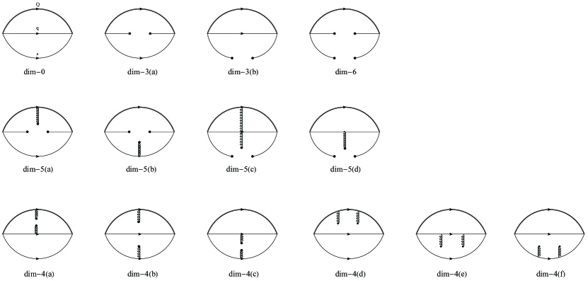
Figure 1: All the diagrams considered in this work. We calculate all these diagrams for the 4 correlation functions $\Pi_{ij}$ with $i,j=0,1$.

The mixing angle formula in Eq. (14) is of course our main research object. However, the corresponding QCD sum rules are very different from the traditional ones: it does not have the hadron-level representation. For this point, try to consider the hadron-level representation of $\Pi_{01}$. That is, Eq. (14) has only a representation at the QCD level. The continuum threshold parameter $\sqrt{s_{0}}$ and Borel parameters $T^{2}$ cannot determined by the methods commonly used in the literature. However, note that a reasonable threshold parameter for Eq. (14) should lie between those of $\Xi_{Q}$ and $\Xi_{Q}^{\prime}$. Naturally, in the following, we present the mass sum rule of $\Xi_{Q}^{(\prime)}$.

II.1 The mass sum rule

Since our preliminary results indicate that $\theta_{c}$ and $\theta_{b}$ are very small, Eqs. (11) and (12) are reduced into

$$\Pi=\Pi_{00}$$ , (17)

$$\Pi^{\prime}=\Pi_{11}$$ . (18)

Following the same steps in Refs. Zhao:2020mod ; Zhao:2021sje , one can perform QCD sum rules analysis on the correlation functions $\Pi_{00,11}$ as follows.

At the hadron level, after inserting the complete set of hadronic states, one can obtain

$$\Pi^{{\rm had}}(p)=\lambda_{+}^{2}\frac{\not{p}+M_{+}}{M_{+}^{2}-p^{2}}+\lambda_{-}^{2}\frac{\not{p}-M_{-}}{M_{-}^{2}-p^{2}}+\cdots,$$ (19)

where $\lambda_{+(-)}$ and $M_{+(-)}$ are respectively the pole residue and mass of the positive-parity (negative-parity) baryon. The pole residues of positive-parity and negative-parity baryons are respectively defined by

$$\langle 0|J_{+}|{\cal B}_{+}(p,s)\rangle =\lambda_{+}u(p,s),$$

$$\langle 0|J_{+}|{\cal B}_{-}(p,s)\rangle =\lambda_{-}(i\gamma_{5})u(p,s).$$ (20)

At the QCD level, the correlation function is also calculated. In this work, contributions from up to dimension-6 four quark operators are considered, as can be seen in Fig. 1. The corresponding results can be formally rewritten as

$$\Pi^{{\rm QCD}}(p)=A(p^{2})\not{p}+B(p^{2}).$$ (21)

The coefficient functions $A(p^{2})$ and $B(p^{2})$ are further written into dispersion relations

$$A(p^{2})=\int ds\frac{\rho^{A}(s)}{s-p^{2}},\quad B(p^{2})=\int ds\frac{\rho^{B}(s)}{s-p^{2}}.$$ (22)

Using the quark-hadron duality assumption, and after performing the Borel transformation, one can arrive at the following sum rule for the positive-parity baryon

$$(M_{+}+M_{-})\lambda_{+}^{2}e^{-M_{+}^{2}/T_{+}^{2}}=\int^{s_{+}}ds(M_{-}\rho^{A}(s)+\rho^{B}(s))e^{-s/T_{+}^{2}},$$ (23)

where $s_{+}$ and $T_{+}^{2}$ are respectively the continuum threshold parameter and Borel parameter. From Eq. (23), one can obtain the mass of the $1/2^{+}$ baryon

$$M_{+}^{2}=\frac{\int^{s_{+}}ds(M_{-}\rho^{A}+\rho^{B})\ s\ e^{-s/T_{+}^{2}}}{\int^{s_{+}}ds(M_{-}\rho^{A}+\rho^{B})\ e^{-s/T_{+}^{2}}}.$$ (24)

In practice, Eq. (24) can be viewed as a constraint of Eq. (23), in which $M_{+}$ is required to be equal to the experimental value of the positive-parity baryon. In this way, the threshold parameter can be determined.

III Numerical results

The following parameters are adopted ParticleDataGroup:2022pth :

$$m_{c}(m_{c})=1.27\pm 0.02\ {\rm GeV},\quad m_{s}(2\ {\rm GeV})=0.093\pm 0.009\ {\rm GeV},$$

$$m_{b}(m_{b})=4.18\pm 0.03\ {\rm GeV}.$$ (25)

The condensate parameters are taken as Colangelo:2000dp : $\langle\bar{q}q\rangle(1\ {\rm GeV})=-(0.24\pm 0.01\ {\rm GeV})^{3}$, $\langle\bar{s}s\rangle=(0.8\pm 0.2)\langle\bar{q}q\rangle$, and $\langle g_{s}^{2}G^{2}\rangle=(0.47\pm 0.14)\ {\rm GeV}^{4}$, and $\langle\bar{q}g_{s}\sigma Gq\rangle=m_{0}^{2}\langle\bar{q}q\rangle$ and $\langle\bar{s}g_{s}\sigma Gs\rangle=m_{0}^{2}\langle\bar{s}s\rangle$ with $m_{0}^{2}=(0.8\pm 0.2)\ {\rm GeV}^{2}$. The renormalization scale is taken as $\mu_{c}=1\sim 3\ {\rm{\rm GeV}}$, and $\mu_{b}=3\sim 6\ {\rm{\rm GeV}}$, from which, one can estimate the dependence of calculation results on the energy scale.

Following similar steps in Refs. Zhao:2020mod ; Zhao:2021sje , one can arrive at the optimal parameter selections for continuum thresholds $\sqrt{s_{0}}$ and Borel parameters $T^{2}$ for $\Xi_{Q}$ and $\Xi_{Q}^{\prime}$. The corresponding results can be found in Fig. 2 and Table 1. Some comments are given in order.

• As expected in Ref. Zhao:2023yuk , the pole residues of $\Xi_{Q}$ and $\Xi_{Q}^{\prime}$ are almost equal when the interpolating currents in Eq. (9) are used.

• The continuum threshold and Borel parameter at the minimum point in Fig. 2 are selected as the optimal parameters, as can be seen in Table 1. These optimal parameters correspond to the experimental value of the baryon mass.

• As can be seen in Table 1, the optimal parameter selection satisfies: $\sqrt{s_{0}}$ is about 0.5 GeV higher than the corresponding baryon mass, and $T^{2}\sim{\cal O}(m_{H}^{2})$ with $m_{H}$ the baryon mass.

• As can be seen in Fig. 2, the dependence of pole residues on the Borel parameters is weak, while they are sensitive to changes in energy scales. The latter leads to the main source of error.

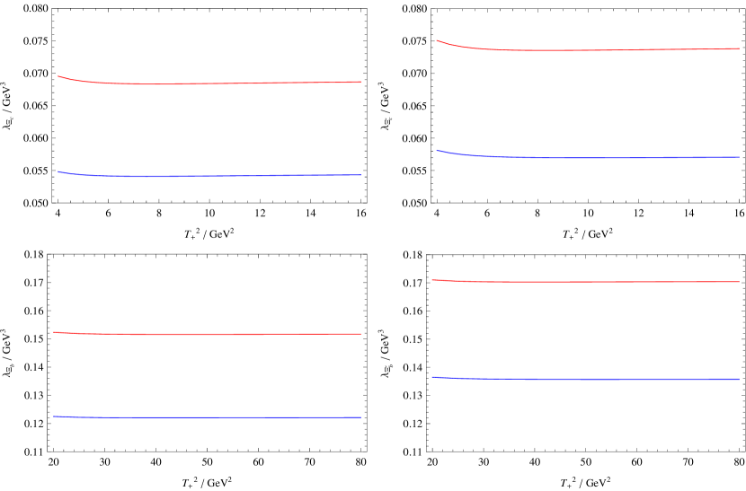
Figure 2: Pole residues of $\Xi_{Q}^{(\prime)}$ with $Q=c,b$. The blue lines correspond to the energy scale $\mu=m_{Q}$, while the red lines correspond to the energy scale $\mu=3\ {\rm GeV}$ for $\Xi_{c}^{(\prime)}$ and $\mu=6\ {\rm GeV}$ for $\Xi_{b}^{(\prime)}$. The selections of $\sqrt{s_{0}}$ can be found in Table 1.

Table 1: Optimal parameter selections for the continuum thresholds $\sqrt{s_{0}}$ and Borel parameters $T^{2}$ for $\Xi_{Q}$ and $\Xi_{Q}^{\prime}$, with $Q=c,b$. The central values are obtained at $\mu=m_{c}$ for $\Xi_{c}^{(\prime)}$ and $\mu=m_{b}$ for $\Xi_{b}^{(\prime)}$. The masses of $\Xi_{c}^{(\prime)0}(csd)$ and $\Xi_{b}^{(\prime)-}(bsd)$ are also listed as references ParticleDataGroup:2022pth .

	$\sqrt{s_{0}}/{\rm GeV}$	$T^{2}/{\rm GeV}^{2}$	Mass/GeV
$\Xi_{c}$	for $\mu=m_{c}$, $2.95$; for $\mu=3\ {\rm GeV}$, $3.00$	$\approx 8$	$2.470$
$\Xi_{c}^{\prime}$	for $\mu=m_{c}$, $3.02$; for $\mu=3\ {\rm GeV}$, $3.10$	$10\pm 2$	$2.579$
$\Xi_{b}$	for $\mu=m_{b}$, $6.27$; for $\mu=6\ {\rm GeV}$, $6.30$	$\approx 40$	$5.797$
$\Xi_{b}^{\prime}$	for $\mu=m_{b}$, $6.40$; for $\mu=6\ {\rm GeV}$, $6.45$	$50\pm 10$	$5.935$

For the sum rule in Eq. (14), considering the continuum threshold should lie between those of $\Xi_{Q}$ and $\Xi_{Q}^{\prime}$, and assuming $T^{2}\sim{\cal O}(m_{H}^{2})$, we choose the following parameters:

• For $\theta_{c}$, when $\mu=m_{c}$, $\sqrt{s_{0}}=2.98\ {\rm GeV}$, and when $\mu=3\ {\rm GeV}$, $\sqrt{s_{0}}=3.05\ {\rm GeV}$; the Borel parameters $T^{2}\in[6,14]\ {\rm GeV}^{2}$.

• For $\theta_{b}$, when $\mu=m_{b}$, $\sqrt{s_{0}}=6.33\ {\rm GeV}$, and when $\mu=6\ {\rm GeV}$, $\sqrt{s_{0}}=6.38\ {\rm GeV}$; the Borel parameters $T^{2}\in[30,70]\ {\rm GeV}^{2}$.

Our main results are shown in Fig. 3, and the corresponding central values and error estimates are:

• $\theta_{c}=(1.3\pm 0.1)\degree$ from the first sum rule, and $\theta_{c}=(2.0\pm 0.8)\degree$ from the second sum rule;

• $\theta_{b}=(0.31\pm 0.03)\degree$ from the first sum rule, and $\theta_{b}=(0.32\pm 0.02)\degree$ from the second sum rule.

Here the first and second sum rules respectively refer to those from the coefficients of $\not{p}$ and constant terms, since all the $\Pi_{ij}$, at the QCD level, can be computed like

$$\Pi^{{\rm QCD}}(p)=A(p^{2})\not{p}+B(p^{2}).$$ (26)

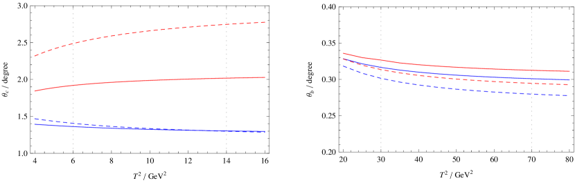
Figure 3: Our predictions for $\theta_{c}$ and $\theta_{b}$. For the left figure, the solid blue and solid red lines respectively represent the curves of $\theta_{c}$ obtained from the first and second sum rules, where $\mu=m_{c}$, $\sqrt{s_{0}}=2.98\ {\rm GeV}$; The blue dashed and red dashed lines respectively represent the curves of $\theta_{c}$ obtained from the first and second sum rules, where $\mu=3\ {\rm GeV}$, $\sqrt{s_{0}}=3.05\ {\rm GeV}$. For the right figure, the solid blue and solid red lines respectively represent the curves of $\theta_{b}$ obtained from the first and second sum rules, where $\mu=m_{b}$, $\sqrt{s_{0}}=6.33\ {\rm GeV}$; The blue dashed and red dashed lines respectively represent the curves of $\theta_{b}$ obtained from the first and second sum rules, where $\mu=6\ {\rm GeV}$, $\sqrt{s_{0}}=6.38\ {\rm GeV}$.

In Table 2, we compare our results with others in the literature. It can be seen that, our result for $\theta_{c}$ is consistent with that of Lattice QCD in Ref. Liu:2023feb if the uncertainty is taken into account.

Table 2: Comparison with other results in the literature (in units of degree). These theoretical predictions respectively come from QCD sum rules (QCDSR), heavy quark effective theory (HQET), Lattice QCD (LQCD), and quark model (QM).

$\theta_{Q}$	This work	QCDSR Aliev:2010ra	HQET Matsui:2020wcc	LQCD Liu:2023feb	QM Franklin:1996ve	QM Franklin:1981rc	HQET Ito:1996mr
$\theta_{c}$	$1.2\sim 2.8$	$5.5\pm 1.8$	$\pm 8.12\pm 0.80$	$1.2\pm 0.1$	$3.8$	$3.8$	$14\pm 14$
$\theta_{b}$	$0.28\sim 0.34$	$6.4\pm 1.8$	$\pm 4.51\pm 0.79$	–	–	$1.0$	–

IV Conclusions and discussions

There is a tension between the recent Belle’s measurement and Lattice QCD calculation for the branching ratio of semileptonic decay ${\cal B}(\Xi_{c}^{0}\to\Xi^{-}e^{+}\nu_{e})$. Some people proposed that it is possible to resolve this puzzle by considering the $\Xi_{Q}-\Xi_{Q}^{\prime}$ mixing. Following this suggestion, we investigate the $\Xi_{Q}-\Xi_{Q}^{\prime}$ mixing using QCD sum rules in this work. Contributions from up to dimension-6 four-quark operators are considered. However, it turns out that only dimension-4 and dimension-5 operators contribute, which reveals the non-perturbative nature of mixing. Especially we notice that only the diagrams with the two light quarks participating in gluon exchange contribute to the mixing. Contributions from three-gluon condensate, and radiative corrections in Fig. 4 may be sizable and deserve further investigation. We leave these more detailed consideration for future works.

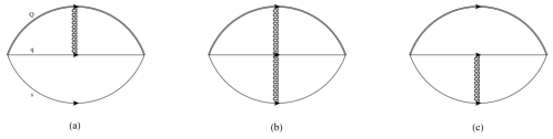
Figure 4: These radiative corrections may play an important rule in $\Xi_{Q}-\Xi_{Q}^{\prime}$ mixing.

Our results show that the mixing angle $\theta_{c}$ is very small, and is consistent with the most recent Lattice QCD calculation result within error. Such a small mixing angle seems unlikely to resolve the tension between experimental measurement and Lattice QCD calculation for the semileptonic decay $\Xi_{c}^{0}\to\Xi^{-}e^{+}\nu_{e}$. We have to draw the conclusion that the tension is still there.

Finally, it is worth pointing out that Ref. Xing:2022phq recently proposed a method for measuring the mixing angle in experiment, which is helpful to further clarify the issue of the $\Xi_{Q}-\Xi_{Q}^{\prime}$ mixing.

Appendix A Analytical Results

In this appendix, we present the calculation results of the correlation functions $\Pi_{00,11,01}$ at the QCD level. Some notes are given below.

• All non-zero results in Fig. 1 are shown in this appendix. The spectral densities $\rho^{A}$ and $\rho^{B}$ are shown together.

• $m_{1}=m_{Q}$ , $m_{2}=m_{q}$, and $m_{3}=m_{s}$, and $m_{2}$ has been taken to be zero. Because we have defined $m_{23}^{2}\equiv k_{23}^{2}\equiv(k_{2}+k_{3})^{2}$ with $k_{2,3}$ respectively the momenta of the light quark $q$ and the strange quark, numeric subscripts are preferable.

• The $m_{23}^{2}$ appearing in the spectral densities of perturbative diagrams (dimension-0) and gluon condensate diagrams (dimension-4) should be integrated out.

• m1s is the $m_{1}^{2}$ that appears on the denominator of the propagator of quark 1. Similar for m2s and m3s.

A.1 Results of $\rho_{00}$

$$\rho_{00}^{{\rm dim-0}}=\frac{3}{32\pi^{6}}\Bigg{\{} \frac{m_{1}^{2}-m_{23}^{2}+s}{6m_{23}^{4}s^{2}}\Big{[}2\left(m_{23}^{2}-m_{3}^{2}\right){}^{2}m_{23}^{2}s$$

$$+6m_{3}\left(m_{23}^{2}-m_{3}^{2}\right)m_{23}^{2}\sqrt{s}\left(-m_{1}^{2}+m_{23}^{2}+s\right)$$

$$+\left(-2m_{3}^{4}+m_{23}^{2}m_{3}^{2}+m_{23}^{4}\right)\left(-m_{1}^{2}+m_{23}^{2}+s\right){}^{2}\Big{]},$$

$$\frac{m_{1}}{3m_{23}^{4}s}\Big{[}2\left(m_{23}^{2}-m_{3}^{2}\right){}^{2}m_{23}^{2}s$$

$$+6m_{3}\left(m_{23}^{2}-m_{3}^{2}\right)m_{23}^{2}\sqrt{s}\left(-m_{1}^{2}+m_{23}^{2}+s\right)$$

$$+\left(-2m_{3}^{4}+m_{23}^{2}m_{3}^{2}+m_{23}^{4}\right)\left(-m_{1}^{2}+m_{23}^{2}+s\right){}^{2}\Big{]}\Bigg{\}}$$

$$\times \frac{\pi\sqrt{\lambda(m_{23}^{2},0,m_{3}^{2})}}{2m_{23}^{2}}\frac{\pi\sqrt{\lambda(s,m_{1}^{2},m_{23}^{2})}}{2s},$$ (27)

$$\rho_{00}^{{\rm dim-3(a)}}=-\frac{\langle\bar{q}q\rangle}{16\pi^{3}}\Bigg{\{} \frac{2\left(m_{1}^{2}-m_{3}^{2}+s\right)\left(\left(m_{3}+\sqrt{s}\right){}^{2}-m_{1}^{2}\right)}{s^{3/2}},$$

$$\frac{4m_{1}\left(\left(m_{3}+\sqrt{s}\right){}^{2}-m_{1}^{2}\right)}{\sqrt{s}}\Bigg{\}}\times\frac{\pi\sqrt{\lambda(s,m_{1}^{2},m_{3}^{2})}}{2s},$$ (28)

$$\rho_{00}^{{\rm dim-3(b)}}=-\frac{\langle\bar{s}s\rangle}{16\pi^{3}}\left\{\frac{2\left(s^{2}-m_{1}^{4}\right)}{s^{3/2}},\frac{4m_{1}\left(s-m_{1}^{2}\right)}{\sqrt{s}}\right\}\times\frac{\pi\sqrt{\lambda(s,m_{1}^{2},0)}}{2s},$$ (29)

$$\rho_{00}^{{\rm dim-4(c)}}= \left(-\frac{\text{$\langle g_{s}^{2}G^{2}\rangle$}}{24576\pi^{6}}\right)\frac{\partial}{\partial\text{m2s}}\frac{\partial}{\partial\text{m3s}}\Bigg{\{}\frac{16\left(m_{1}^{2}-m_{23}^{2}+s\right)}{s^{2}}\Big{[}-\frac{1}{6m_{23}^{4}}$$

$$\times\Big{(}\left(-m_{1}^{2}+m_{23}^{2}+s\right){}^{2}\left(m_{23}^{4}+m_{23}^{2}(\text{m2s}+\text{m3s})-2(\text{m2s}-\text{m3s})^{2}\right)$$

$$\quad+2m_{23}^{2}s\left(m_{23}^{4}-2m_{23}^{2}(\text{m2s}+\text{m3s})+(\text{m2s}-\text{m3s})^{2}\right)\Big{)}$$

$$-\frac{3m_{3}\sqrt{s}\left(-m_{1}^{2}+m_{23}^{2}+s\right)(m_{23}^{2}+\text{m2s}-\text{m3s})}{m_{23}^{2}}$$

$$-4s(m_{23}^{2}-\text{m2s}-\text{m3s})\Big{]},$$

$$32m_{1}\Big{[}-\frac{1}{6m_{23}^{4}s}$$

$$\times\Big{(}\left(-m_{1}^{2}+m_{23}^{2}+s\right){}^{2}\left(m_{23}^{2}(\text{m2s}+\text{m3s})+m_{23}^{4}-2(\text{m2s}-\text{m3s})^{2}\right)$$

$$\quad+2m_{23}^{2}s\left(m_{23}^{4}-2m_{23}^{2}(\text{m2s}+\text{m3s})+(\text{m2s}-\text{m3s})^{2}\right)\Big{)}$$

$$-\frac{3m_{3}\left(-m_{1}^{2}+m_{23}^{2}+s\right)\left(m_{23}^{2}+\text{m2s}-\text{m3s}\right)}{m_{23}^{2}\sqrt{s}}$$

$$-4\left(m_{23}^{2}-\text{m2s}-\text{m3s}\right)\Big{]}\Bigg{\}}$$

$$\times \frac{\pi\sqrt{\lambda(m_{23}^{2},\text{m2s},\text{m3s})}}{2m_{23}^{2}}\frac{\pi\sqrt{\lambda(s,m_{1}^{2},m_{23}^{2})}}{2s},$$ (30)

$$\rho_{00}^{{\rm dim-4(d)}}= \frac{\langle g_{s}^{2}G^{2}\rangle}{128\pi^{6}}\frac{1}{6}\frac{\partial^{3}}{\partial\text{m1s}^{3}}\Bigg{\{}\frac{m_{1}^{2}\left(-m_{23}^{2}+\text{m1s}+s\right)}{6m_{23}^{4}s^{2}}$$

$$\times\Big{[}6m_{3}\left(m_{23}^{2}-m_{3}^{2}\right)m_{23}^{2}\sqrt{s}\left(m_{23}^{2}-\text{m1s}+s\right)$$

$$\quad+\left(-2m_{3}^{4}+m_{23}^{2}m_{3}^{2}+m_{23}^{4}\right)\left(m_{23}^{2}-\text{m1s}+s\right){}^{2}$$

$$\quad+2\left(m_{23}^{2}-m_{3}^{2}\right){}^{2}m_{23}^{2}s\Big{]},$$

$$\frac{m_{1}\text{m1s}}{3m_{23}^{4}s}$$

$$\times\Big{[}6m_{3}\left(m_{23}^{2}-m_{3}^{2}\right)m_{23}^{2}\sqrt{s}\left(m_{23}^{2}-\text{m1s}+s\right)$$

$$\quad+\left(-2m_{3}^{4}+m_{23}^{2}m_{3}^{2}+m_{23}^{4}\right)\left(m_{23}^{2}-\text{m1s}+s\right){}^{2}$$

$$\quad+2\left(m_{23}^{2}-m_{3}^{2}\right){}^{2}m_{23}^{2}s\Big{]}\Bigg{\}}$$

$$\times \frac{\pi\sqrt{\lambda(m_{23}^{2},0,m_{3}^{2})}}{2m_{23}^{2}}\frac{\pi\sqrt{\lambda(s,\text{m1s},m_{23}^{2})}}{2s},$$ (31)

$$\rho_{00}^{{\rm dim-5(b)}}= \left(-\frac{\langle\bar{q}g_{s}\sigma Gq\rangle}{1536\pi^{3}}\right)\frac{\partial}{\partial\text{m3s}}\Bigg{\{}-\frac{24\left(m_{1}^{2}-\text{m3s}+s\right)\left(2m_{3}\sqrt{s}-m_{1}^{2}+\text{m3s}+s\right)}{s^{3/2}},$$

$$-4m_{1}\left(\frac{12\left(-m_{1}^{2}+\text{m3s}+s\right)}{\sqrt{s}}+24m_{3}\right)\Bigg{\}}\frac{\pi\sqrt{\lambda(s,m_{1}^{2},\text{m3s})}}{2s},$$ (32)

$$\rho_{00}^{{\rm dim-5(d)}}=\left(-\frac{\langle\bar{s}g_{s}\sigma Gs\rangle}{1536\pi^{3}}\right)\frac{\partial}{\partial\text{m2s}}\Bigg{\{} -\frac{24\left(-m_{1}^{2}+\text{m2s}+s\right)\left(m_{1}^{2}-\text{m2s}+s\right)}{s^{3/2}},$$

$$-\frac{48m_{1}\left(-m_{1}^{2}+\text{m2s}+s\right)}{\sqrt{s}}\Bigg{\}}\frac{\pi\sqrt{\lambda(s,m_{1}^{2},\text{m2s})}}{2s},$$ (33)

$$\rho_{00}^{{\rm dim-6}}=\left(\frac{\langle\bar{q}q\rangle\langle\bar{s}s\rangle}{24}\right)\{8,8m_{1}\}\delta(s-m_{1}^{2}).$$ (34)

A.2 Results of $\rho_{11}$

$$\rho_{11}^{{\rm dim-0}} =\rho_{00}^{{\rm dim-0}},$$ (35)

$$\rho_{11}^{{\rm dim-3(a)}} =\rho_{00}^{{\rm dim-3(a)}},$$ (36)

$$\rho_{11}^{{\rm dim-3(b)}} =\rho_{00}^{{\rm dim-3(b)}},$$ (37)

$$\rho_{11}^{{\rm dim-4}(a)}= \left(-\frac{\langle g_{s}^{2}G^{2}\rangle}{24576\pi^{6}}\right)\frac{\partial}{\partial\text{m1s}}\frac{\partial}{\partial\text{m2s}}\Bigg{\{}-\frac{16}{9m_{23}^{4}s}$$

$$\times\Big{[}-24m_{3}m_{23}^{2}\sqrt{s}\left(-m_{3}^{2}+m_{23}^{2}+\text{m2s}\right)\left(m_{23}^{2}+\text{m1s}-s\right)$$

$$+\frac{6m_{3}m_{23}^{2}\left(-m_{3}^{2}+m_{23}^{2}+\text{m2s}\right)\left(m_{23}^{2}-\text{m1s}+s\right)\left(-m_{23}^{2}+\text{m1s}+s\right)}{\sqrt{s}}$$

$$+4\Big{(}m_{23}^{2}\left(-2m_{3}^{2}\left(m_{23}^{2}+\text{m2s}\right)+\left(m_{23}^{2}-\text{m2s}\right){}^{2}+m_{3}^{4}\right)\left(-m_{23}^{2}+\text{m1s}+s\right)$$

$$\quad+\left(m_{23}^{2}\left(m_{3}^{2}+\text{m2s}\right)-2\left(\text{m2s}-m_{3}^{2}\right){}^{2}+m_{23}^{4}\right)$$

$$\qquad\times\left(-m_{23}^{2}-\text{m1s}+s\right)\left(m_{23}^{2}-\text{m1s}+s\right)\Big{)}$$

$$+\frac{\left(-m_{23}^{2}+\text{m1s}+s\right)}{s}$$

$$\times\Big{(}\left(m_{23}^{2}\left(m_{3}^{2}+\text{m2s}\right)-2\left(\text{m2s}-m_{3}^{2}\right){}^{2}+m_{23}^{4}\right)\left(m_{23}^{2}-\text{m1s}+s\right){}^{2}$$

$$\quad+2m_{23}^{2}s\left(-2m_{3}^{2}\left(m_{23}^{2}+\text{m2s}\right)+\left(m_{23}^{2}-\text{m2s}\right){}^{2}+m_{3}^{4}\right)\Big{)}\Big{]},$$

$$-\frac{32m_{1}}{3m_{23}^{4}s}$$

$$\times\Big{[}\left(m_{23}^{2}\left(m_{3}^{2}+\text{m2s}\right)-2\left(\text{m2s}-m_{3}^{2}\right){}^{2}+m_{23}^{4}\right)\left(m_{23}^{2}-\text{m1s}+s\right){}^{2}$$

$$\quad+6m_{3}m_{23}^{2}\sqrt{s}\left(-m_{3}^{2}+m_{23}^{2}+\text{m2s}\right)\left(m_{23}^{2}-\text{m1s}+s\right)$$

$$\quad+2m_{23}^{2}s\left(-2m_{3}^{2}\left(m_{23}^{2}+\text{m2s}\right)+\left(m_{23}^{2}-\text{m2s}\right){}^{2}+m_{3}^{4}\right)\Big{]}\Bigg{\}}$$

$$\times \frac{\pi\sqrt{\lambda(m_{23}^{2},\text{m2s},m_{3}^{2})}}{2m_{23}^{2}}\frac{\pi\sqrt{\lambda(s,\text{m1s},m_{23}^{2})}}{2s},$$ (38)

$$\rho_{11}^{{\rm dim-4(b)}}= \left(-\frac{\langle g_{s}^{2}G^{2}\rangle}{24576\pi^{6}}\right)\frac{\partial}{\partial\text{m1s}}\frac{\partial}{\partial\text{m3s}}\Bigg{\{}\frac{16}{9m_{23}^{4}s}$$

$$\times\Big{[}\frac{2\left(m_{23}^{2}\text{m3s}+m_{23}^{4}-2\text{m3s}^{2}\right)\left(-m_{23}^{2}+\text{m1s}+s\right)\left(m_{23}^{2}-\text{m1s}+s\right){}^{2}}{s}$$

$$\quad+4\left(m_{23}^{2}\text{m3s}+m_{23}^{4}-2\text{m3s}^{2}\right)\left(m_{23}^{2}+\text{m1s}-s\right)\left(m_{23}^{2}-\text{m1s}+s\right)$$

$$\quad-\frac{3\left(-m_{23}^{2}+\text{m1s}+s\right)}{s}\Big{(}\left(m_{23}^{2}\text{m3s}+m_{23}^{4}-2\text{m3s}^{2}\right)\left(m_{23}^{2}-\text{m1s}+s\right){}^{2}$$

$$\qquad+2m_{23}^{2}s\left(m_{23}^{2}-\text{m3s}\right){}^{2}\Big{)}$$

$$\quad-\frac{18m_{3}m_{23}^{2}\left(m_{23}^{2}-\text{m3s}\right)\left(-m_{23}^{2}+\text{m1s}+s\right)\left(m_{23}^{2}-\text{m1s}+s\right)}{\sqrt{s}}\Big{]},$$

$$-\frac{32m_{1}\left(m_{23}^{2}-\text{m3s}\right)}{3m_{23}^{4}s}$$

$$\times\Big{[}\text{m1s}^{2}\left(m_{23}^{2}+2\text{m3s}\right)-2\text{m1s}\left(m_{23}^{2}+2\text{m3s}\right)\left(m_{23}^{2}+s\right)$$

$$\quad+6m_{3}m_{23}^{2}\sqrt{s}\left(m_{23}^{2}-\text{m1s}+s\right)+2m_{23}^{2}\text{m3s}s+2m_{23}^{4}\text{m3s}$$

$$\quad+m_{23}^{2}s^{2}+4m_{23}^{4}s+m_{23}^{6}+2\text{m3s}s^{2}\Big{]}\Bigg{\}}$$

$$\times \frac{\pi\sqrt{\lambda(m_{23}^{2},0,\text{m3s})}}{2m_{23}^{2}}\frac{\pi\sqrt{\lambda(s,\text{m1s},m_{23}^{2})}}{2s},$$ (39)

$$\rho_{11}^{{\rm dim-4(c)}} =-\frac{1}{3}\rho_{00}^{{\rm dim-4(c)}},$$ (40)

$$\rho_{11}^{{\rm dim-4(d)}} =\rho_{00}^{{\rm dim-4(d)}},$$ (41)

$$\rho_{11}^{{\rm dim-5(a)}}= \left(-\frac{\langle\bar{q}g_{s}\sigma Gq\rangle}{1536\pi^{3}}\right)\frac{\partial}{\partial\text{m1s}}\Bigg{\{}-\frac{16\left(-m_{3}^{2}+\text{m1s}+s\right)\left(2m_{3}\sqrt{s}+m_{3}^{2}-\text{m1s}+s\right)}{s^{3/2}},$$

$$-\frac{32m_{1}\left(2m_{3}\sqrt{s}+m_{3}^{2}-\text{m1s}+s\right)}{\sqrt{s}}\Bigg{\}}\frac{\pi\sqrt{\lambda(s,\text{m1s},m_{3}^{2})}}{2s},$$ (42)

$$\rho_{11}^{{\rm dim-5(b)}}=-\frac{1}{3}\rho_{00}^{{\rm dim-5(b)}},$$ (43)

$$\rho_{11}^{{\rm dim-5(c)}}=\left(-\frac{\langle\bar{s}g_{s}\sigma Gs\rangle}{1536\pi^{3}}\right)\frac{\partial}{\partial\text{m1s}} \Bigg{\{}\frac{16(\text{m1s}-s)(\text{m1s}+s)}{s^{3/2}},\frac{32m_{1}(\text{m1s}-s)}{\sqrt{s}}\Bigg{\}}$$

$$\times\frac{\pi\sqrt{\lambda(s,\text{m1s},0)}}{2s},$$ (44)

$$\rho_{11}^{{\rm dim-5(d)}}=-\frac{1}{3}\rho_{00}^{{\rm dim-5(d)}},$$ (45)

$$\rho_{11}^{{\rm dim-6}}=\rho_{00}^{{\rm dim-6}}.$$ (46)

A.3 Results of $\rho_{01}$

$$\rho_{01}^{{\rm dim-5(a)}}= \left(-\frac{\langle\bar{q}g_{s}\sigma Gq\rangle}{1536\pi^{3}}\right)\frac{\partial}{\partial\text{m1s}}\Bigg{\{}-\frac{16\sqrt{3}m_{1}\left(2m_{3}\sqrt{s}+m_{3}^{2}-\text{m1s}+s\right)}{s},$$

$$-\frac{8\sqrt{3}\left(-m_{3}^{2}+\text{m1s}+s\right)\left(2m_{3}\sqrt{s}+m_{3}^{2}-\text{m1s}+s\right)}{s}\Bigg{\}}\frac{\pi\sqrt{\lambda(s,\text{m1s},m_{3}^{2})}}{2s},$$ (47)

$$\rho_{01}^{{\rm dim-5(c)}}=\left(-\frac{\langle\bar{s}g_{s}\sigma Gs\rangle}{1536\pi^{3}}\right)\frac{\partial}{\partial\text{m1s}} \Bigg{\{}\frac{16\sqrt{3}m_{1}(s-\text{m1s})}{s},\frac{8\sqrt{3}(s-\text{m1s})(\text{m1s}+s)}{s}\Bigg{\}}$$

$$\times\frac{\pi\sqrt{\lambda(s,\text{m1s},0)}}{2s},$$ (48)

$$\rho_{01}^{{\rm dim-4(a)}}= \left(-\frac{\text{$\langle g_{s}^{2}G^{2}\rangle$}}{24576\pi^{6}}\right)\frac{\partial}{\partial\text{m1s}}\frac{\partial}{\partial\text{m2s}}\Bigg{\{}-\frac{16m_{1}}{\sqrt{3}m_{23}^{4}s}$$

$$\times\Big{[}6m_{3}m_{23}^{2}\left(-m_{3}^{2}+m_{23}^{2}+\text{m2s}\right)\left(m_{23}^{2}-\text{m1s}+s\right)$$

$$\quad+\frac{1}{\sqrt{s}}\Big{(}\left(m_{23}^{2}\left(m_{3}^{2}+\text{m2s}\right)-2\left(\text{m2s}-m_{3}^{2}\right){}^{2}+m_{23}^{4}\right)\left(m_{23}^{2}-\text{m1s}+s\right){}^{2}$$

$$\qquad+2m_{23}^{2}s\left(-2m_{3}^{2}\left(m_{23}^{2}+\text{m2s}\right)+\left(m_{23}^{2}-\text{m2s }\right){}^{2}+m_{3}^{4}\right)\Big{)}\Big{]},$$

$$-\frac{8}{3\sqrt{3}m_{23}^{4}}\Big{[}\frac{\left(-m_{23}^{2}+\text{m1s}+s\right)}{s^{3/2}}$$

$$\quad\times\Big{(}\left(m_{23}^{2}\left(m_{3}^{2}+\text{m2s}\right)-2\left(\text{m2s}-m_{3}^{2}\right){}^{2}+m_{23}^{4}\right)\left(m_{23}^{2}-\text{m1s}+s\right){}^{2}$$

$$\qquad+2m_{23}^{2}s\left(-2m_{3}^{2}\left(m_{23}^{2}+\text{m2s}\right)+\left(m_{23}^{2}-\text{m2s}\right){}^{2}+m_{3}^{4}\right)\Big{)}$$

$$\quad-24m_{3}m_{23}^{2}\left(-m_{3}^{2}+m_{23}^{2}+\text{m2s}\right)\left(m_{23}^{2}+\text{m1s}-s\right)$$

$$\quad+\frac{6m_{3}m_{23}^{2}\left(-m_{3}^{2}+m_{23}^{2}+\text{m2s}\right)\left(m_{23}^{2}-\text{m1s}+s\right)\left(-m_{23}^{2}+\text{m1s}+s\right)}{s}$$

$$\quad+\frac{4}{\sqrt{s}}\Big{(}m_{23}^{2}\left(-2m_{3}^{2}\left(m_{23}^{2}+\text{m2s}\right)+\left(m_{23}^{2}-\text{m2s}\right){}^{2}+m_{3}^{4}\right)\left(-m_{23}^{2}+\text{m1s}+s\right)$$

$$\qquad+\left(m_{23}^{2}\left(m_{3}^{2}+\text{m2s}\right)-2\left(\text{m2s}-m_{3}^{2}\right){}^{2}+m_{23}^{4}\right)$$

$$\qquad\quad\times\left(-m_{23}^{2}-\text{m1s}+s\right)\left(m_{23}^{2}-\text{m1s}+s\right)\Big{)}\Big{]}\Bigg{\}}$$

$$\times \frac{\pi\sqrt{\lambda(m_{23}^{2},\text{m2s},m_{3}^{2})}}{2m_{23}^{2}}\frac{\pi\sqrt{\lambda(s,\text{m1s},m_{23}^{2})}}{2s},$$ (49)

$$\rho_{01}^{{\rm dim-4(b)}}= \left(-\frac{\langle g_{s}^{2}G^{2}\rangle}{24576\pi^{6}}\right)\frac{\partial}{\partial\text{m1s}}\frac{\partial}{\partial\text{m3s}}\Bigg{\{}\frac{16m_{1}}{\sqrt{3}m_{23}^{4}s}$$

$$\times\Big{[}\frac{\left(m_{23}^{2}\text{m3s}+m_{23}^{4}-2\text{m3s}^{2}\right)\left(m_{23}^{2}-\text{m1s}+s\right){}^{2}+2m_{23}^{2}s\left(m_{23}^{2}-\text{m3s}\right){}^{2}}{\sqrt{s}}$$

$$\quad+6m_{3}m_{23}^{2}\left(m_{23}^{2}-\text{m3s}\right)\left(m_{23}^{2}-\text{m1s}+s\right)\Big{]},$$

$$\frac{8}{3\sqrt{3}m_{23}^{4}s^{3/2}}$$

$$\times\Big{[}4s\Big{(}m_{23}^{2}\left(m_{23}^{2}-\text{m3s}\right){}^{2}\left(-m_{23}^{2}+\text{m1s}+s\right)$$

$$\qquad-\left(m_{23}^{2}\text{m3s}+m_{23}^{4}-2\text{m3s}^{2}\right)\left(m_{23}^{2}+\text{m1s}-s\right)\left(m_{23}^{2}-\text{m1s}+s\right)\Big{)}$$

$$\quad+\left(-m_{23}^{2}+\text{m1s}+s\right)\Big{(}\left(m_{23}^{2}\text{m3s}+m_{23}^{4}-2\text{m3s}^{2}\right)\left(m_{23}^{2}-\text{m1s}+s\right){}^{2}$$

$$\qquad+2m_{23}^{2}s\left(m_{23}^{2}-\text{m3s}\right){}^{2}\Big{)}$$

$$\quad+18m_{3}m_{23}^{2}\sqrt{s}\left(m_{23}^{2}-\text{m3s}\right)\left(-m_{23}^{2}+\text{m1s}+s\right)\left(m_{23}^{2}-\text{m1s}+s\right)\Big{]}\Bigg{\}}$$

$$\times \frac{\pi\sqrt{\lambda(m_{23}^{2},0,\text{m3s})}}{2m_{23}^{2}}\frac{\pi\sqrt{\lambda(s,\text{m1s},m_{23}^{2})}}{2s}.$$ (50)

References

• (1) Y. B. Li et al. [Belle], Phys. Rev. Lett. 127, no.12, 121803 (2021) doi:10.1103/PhysRevLett.127.121803 [arXiv:2103.06496 [hep-ex]].
• (2) Q. A. Zhang, J. Hua, F. Huang, R. Li, Y. Li, C. Lü, C. D. Lu, P. Sun, W. Sun and W. Wang, et al. Chin. Phys. C 46, no.1, 011002 (2022) doi:10.1088/1674-1137/ac2b12 [arXiv:2103.07064 [hep-lat]].
• (3) Z. X. Zhao, [arXiv:2103.09436 [hep-ph]].
• (4) X. G. He, F. Huang, W. Wang and Z. P. Xing, Phys. Lett. B 823, 136765 (2021) doi:10.1016/j.physletb.2021.136765 [arXiv:2110.04179 [hep-ph]].
• (5) C. Q. Geng, X. N. Jin, C. W. Liu, X. Yu and A. W. Zhou, Phys. Lett. B 839, 137831 (2023) doi:10.1016/j.physletb.2023.137831 [arXiv:2212.02971 [hep-ph]].
• (6) C. Q. Geng, X. N. Jin and C. W. Liu, Phys. Lett. B 838, 137736 (2023) doi:10.1016/j.physletb.2023.137736 [arXiv:2210.07211 [hep-ph]].
• (7) H. W. Ke and X. Q. Li, Phys. Rev. D 105, no.9, 9 (2022) doi:10.1103/PhysRevD.105.096011 [arXiv:2203.10352 [hep-ph]].
• (8) T. M. Aliev, A. Ozpineci and V. Zamiralov, Phys. Rev. D 83, 016008 (2011) doi:10.1103/PhysRevD.83.016008 [arXiv:1007.0814 [hep-ph]].
• (9) Y. Matsui, Nucl. Phys. A 1008, 122139 (2021) doi:10.1016/j.nuclphysa.2021.122139 [arXiv:2011.09653 [hep-ph]].
• (10) H. Liu, L. Liu, P. Sun, W. Sun, J. X. Tan, W. Wang, Y. B. Yang and Q. A. Zhang, [arXiv:2303.17865 [hep-lat]].
• (11) Z. X. Zhao, F. W. Zhang, X. H. Hu and Y. J. Shi, Phys. Rev. D 107, no.11, 116025 (2023) doi:10.1103/PhysRevD.107.116025 [arXiv:2304.07698 [hep-ph]].
• (12) R. L. Workman et al. [Particle Data Group], PTEP 2022, 083C01 (2022) doi:10.1093/ptep/ptac097
• (13) P. Colangelo and A. Khodjamirian, doi:10.1142/9789812810458_0033 [arXiv:hep-ph/0010175 [hep-ph]].
• (14) Z. X. Zhao, R. H. Li, Y. L. Shen, Y. J. Shi and Y. S. Yang, Eur. Phys. J. C 80, no.12, 1181 (2020) doi:10.1140/epjc/s10052-020-08767-1 [arXiv:2010.07150 [hep-ph]].
• (15) J. Franklin, Phys. Rev. D 55, 425-426 (1997) doi:10.1103/PhysRevD.55.425 [arXiv:hep-ph/9606326 [hep-ph]].
• (16) J. Franklin, D. B. Lichtenberg, W. Namgung and D. Carydas, Phys. Rev. D 24, 2910 (1981) doi:10.1103/PhysRevD.24.2910
• (17) T. Ito and Y. Matsui, Prog. Theor. Phys. 96, 659-664 (1996) doi:10.1143/PTP.96.659 [arXiv:hep-ph/9605289 [hep-ph]].
• (18) Z. P. Xing and Y. j. Shi, Phys. Rev. D 107, no.7, 074024 (2023) doi:10.1103/PhysRevD.107.074024 [arXiv:2212.09003 [hep-ph]].