Levenberg-Marquardt method with Singular Scaling and applications

Abstract

Inspired by certain regularization techniques for linear inverse problems, in this work we investigate the convergence properties of the Levenberg-Marquardt method using singular scaling matrices. Under a completeness condition, we show that the method is well-defined and establish its local quadratic convergence under an error bound assumption. We also prove that the search directions are gradient-related allowing us to show that limit points of the sequence generated by a line-search version of the method are stationary for the sum-of-squares function. The usefulness of the method is illustrated with some examples of parameter identification in heat conduction problems for which specific singular scaling matrices can be used to improve the quality of approximate solutions.

Keywords. Levenberg-Marquardt, Singular Scaling Matrix, Convergence analysis, Parameter identification

1 Introduction

In this work we consider the following nonlinear least-squares problem

$$\min_{x\in\mathbb{R}^{n}}\frac{1}{2}\|F(x)\|_{2}^{2}=:\phi(x),$$ (1)

where $F:\mathbb{R}^{n}\rightarrow\mathbb{R}^{m}$ is continuously differentiable. Throughout this paper we assume that the optimal value for (1) is zero, i.e. the set

$$X^{*}:=\{x\in\mathbb{R}^{n}\mid F(x)=\textbf{{0}}\}$$

is non-empty.

We shall provide local and global convergence analysis for the following Levenberg-Marquardt method (LMM)

$$(J_{k}^{T}J_{k}+\lambda_{k}L^{T}L)d_{k} =-J_{k}^{T}F_{k}$$ (2)

$$x_{k+1} =x_{k}+\alpha_{k}d_{k},\quad\forall k\geq 0,$$ (3)

where $F_{k}:=F(x_{k})$, $J_{k}:=J(x_{k})$ is the Jacobian of $F$ at $x_{k}$, $\{\lambda_{k}\}$ is a sequence of positive scalars and $\{\alpha_{k}\}$ corresponds to a step-size sequence.

In the classic LMM, instead of $L^{T}L$ a positive definite matrix $D_{k}$ called scaling matrix is usually chosen. Convergence theory for this case and, in particular, for the choice $D_{k}=I_{n}$, the identity matrix, is well-known in the literature and local quadratic convergence can be shown under mild assumptions [26, 25, 48, 33, 28, 31, 8, 7].

In this work however, motivated by applications in inverse problems, we choose the scaling matrix in the form $D_{k}=L^{T}L$ and allow it to be singular. We shall refer to the iteration (2)–(3) as Levenberg-Marquardt method with Singular Scaling (LMMSS).

Several authors over the decades have proposed different choices for the scaling matrix, with $D_{k}$ non-singular, showing advantages on the generated approximations made by LMM. Emblematic examples generally take $D_{k}$ as diagonal [19], for instance, Moré [33] introduces information from the Jacobian $J_{k}$ on this diagonal in the iterative process, aiming to help convergence and improve the conditioning of (2). Other definitions of $D_{k}$, which vary according to the context of the problem, may be found in [25, 49, 43, 17, 45, 35, 36].

On the other hand, our motivation to use singular matrices in the form $L^{T}L$ comes from the general form Tikhonov regularization [44] for linear systems $Ax=b$, i.e.,

$$x_{\lambda}=(A^{T}A+\lambda L^{T}L)^{-1}A^{T}b.$$

In this case, the literature indicates that for discrete ill-posed problems with smooth solution, the choice of $L$ as a discrete version of derivative operators can lead to significant improvements in the generated approximations [20, 21].

Hence, in this paper the use of a singular, and constant, $D_{k}=L^{T}L$ is not directly related to improving the conditioning of LMM subproblem or speeding-up convergence, but rather to allow us to introduce desired properties, e.g. smoothness, in the solution obtained by LMM in certain inverse problems. Our aim is to show that convergence of LMM with such singular scaling matrices can still be achieved under reasonable assumptions and that the use of certain problem-oriented singular scaling matrices has an impact in the quality of the obtained approximate solutions.

As far as we know, there are no works in the literature treating local and global convergence of LMM with singular scaling matrices. Although the roadmap of the convergence analysis follows closely the seminal work [48], there are new challenges imposed by the singularity of the scaling matrices in the proof of key lemmas that demands other theoretical tools and additional assumptions.

This paper is organized as follows. In Section 2, we start by presenting the mathematical background and preliminary results necessary to the upcoming sections. Under a completeness condition we show that the LMMSS iteration is well-defined and prove its local quadratic convergence under an error bound condition in Section 3. Next, we prove in Section 4 that, for LMMSS with an Armijo line-search scheme, every limit point of the generated sequence is a stationary point of the sum-of-squares function. Finally, Section 5 presents several examples of parameter identification on heat conduction problems in which specific singular scaling matrices tend to be effective. The paper ends with final remarks and future perspectives in Section 6.

2 Preliminaries and auxiliary results

In this section we present the assumptions needed in the convergence analysis and recall some facts about the generalized singular value decomposition that are useful to establish some auxiliary lemmas.

Let $B(\bar{x},\rho)$ denotes a closed ball in $\mathbb{R}^{n}$ centered at $\bar{x}$ with radius $\rho$ and $\mathcal{N}(A)$ the null-space of a matrix $A$. Concerning the linear system (2) and the matrix $L\in\mathbb{R}^{p\times n}$ we consider the following assumption.

Assumption 1.

The matrix $L\in\mathbb{R}^{p\times n}$ is full-rank, where $m\geq n\geq p$, and there exist $\gamma>0$ such that, for every $x\in\mathbb{R}^{n}$

$$\|J(x)v\|_{2}^{2}+\|Lv\|_{2}^{2}\geq\gamma\|v\|_{2}^{2},\quad\forall v\in\mathbb{R}^{n}.$$ (4)

Inequality (4) is related to the completeness condition, well-known in the inverse problems literature (see [34, p. 34] and [16, p. 197]). We remark that Assumption 1 is equivalent to

$$\mathcal{N}(J(x))\cap\mathcal{N}(L)=\{\textbf{{0}}\},\quad\forall x\in\mathbb{R}^{n}.$$ (5)

Condition (5) allows us to show that, for $\lambda_{k}>0$, $(J_{k}^{T}J_{k}+\lambda_{k}L^{T}L)$ is symmetric positive definite and thus the linear system (2) has a unique solution $d_{k}$. Moreover, $d_{k}$ coincides with the unique minimizer of the following quadratic model

$$\theta_{k}(d)=\|J_{k}d+F_{k}\|_{2}^{2}+\lambda_{k}\|Ld\|_{2}^{2}.$$ (6)

Motivated by the analysis in [48], we also assume that the Levenberg-Marquardt parameter (damping parameter) $\lambda_{k}$ is chosen as follows.

Assumption 2.

The damping parameter is chosen as $\lambda_{k}=\lambda(x_{k}):=\|F(x_{k})\|_{2}^{2}$, for every $k\geq 0$.

An useful tool for analyzing the matrix pair $(J_{k},L)$ involved in LMMSS iterations is the generalized singular value decomposition (GSVD). It was introduced by Van Loan [46] and further developed in subsequent works [47, 39]. Here we present it according to [20, p. 22]. For a proof and other properties we recommend [10].

Theorem 2.1 (GSVD, Hansen [20, p. 22]).

Consider a matrix pair $(A,L)$, where $A\in\mathbb{R}^{m\times n}$, $L\in\mathbb{R}^{p\times n}$, $m\geq n\geq p$, $\textup{rank}(L)=p$ and $\mathcal{N}(A)\cap\mathcal{N}(L)=\{\textbf{{0}}\}$. Then, there exist matrices $U\in\mathbb{R}^{m\times n}$ and $V\in\mathbb{R}^{p\times p}$ with orthonormal columns and a non-singular $X\in\mathbb{R}^{n\times n}$ such that

$$A=U\left[\begin{array}[]{cc}\Sigma&\textbf{{0}}\\ \textbf{{0}}&I_{n-p}\end{array}\right]X^{-1}\qquad\text{and}\qquad L=V\left[\begin{array}[]{cc}M&\textbf{{0}}\end{array}\right]X^{-1},$$ (7)

where $\Sigma$ and $M$ are diagonal matrices:

$$\Sigma=\operatorname*{diag}(\sigma_{1},\dots,\sigma_{p})\in\mathbb{R}^{p\times p}\quad\text{and}\quad M=\operatorname*{diag}(\mu_{1},\dots,\mu_{p})\in\mathbb{R}^{p\times p}.$$ (8)

Moreover, the diagonal elements of $\Sigma$ and $M$ are non-negative, ordered such that

$$0\leq\sigma_{1}\leq\dots\leq\sigma_{p}\leq 1\quad\text{and}\quad 1\geq\mu_{1}\geq\dots\geq\mu_{p}>0$$ (9)

and normalized by the relation $\sigma_{i}^{2}+\mu_{i}^{2}=1$, for $i=1,\dots,p$. The quotients

$$\gamma_{i}=\frac{\sigma_{i}}{\mu_{i}},\quad i=1,\dots,p,$$

are called generalized singular values of the pair $(A,L)$.

GSVD of the pair $(J_{k},L)$ gives us a precise characterization of the direction $d_{k}$ in LMMSS. In fact, given the GSVD

$$J_{k}=U_{k}\left[\begin{array}[]{cc}\Sigma_{k}&\textbf{{0}}\\ \textbf{{0}}&I_{n-p}\end{array}\right]X_{k}^{-1}\quad\text{and}\quad L=V_{k}\left[\begin{array}[]{cc}M_{k}&\textbf{{0}}\end{array}\right]X_{k}^{-1},$$

where

$$(\Sigma_{k})_{ii}:=\sigma_{i,k}\quad\text{and}\quad(M_{k})_{ii}:=\mu_{i,k},\quad i=1,\dots,p,$$

we obtain

$$J_{k}^{T}J_{k}+\lambda_{k}L^{T}L=X_{k}^{-T}\left[\begin{array}[]{cc}\Sigma_{k}^{2}+\lambda_{k}M_{k}^{2}&\textbf{{0}}\\ \textbf{{0}}&I_{n-p}\end{array}\right]X_{k}^{-1}.$$ (10)

Then, $d_{k}$ from (2) can be expressed as

$$d_{k}=-X_{k}\left[\begin{array}[]{cc}(\Sigma_{k}^{2}+\lambda_{k}M_{k}^{2})^{-1}&\textbf{{0}}\\ \textbf{{0}}&I_{n-p}\end{array}\right]X_{k}^{T}\left(X_{K}^{-T}\left[\begin{array}[]{cc}\Sigma_{k}&\textbf{{0}}\\ \textbf{{0}}&I_{n-p}\end{array}\right]U_{k}^{T}\right)F_{k},$$

and further reduced to

$$d_{k}=-X_{k}\left[\begin{array}[]{cc}\Gamma_{k}&\textbf{{0}}\\ \textbf{{0}}&I_{n-p}\end{array}\right]U_{k}^{T}F_{k},\quad\text{where}\quad\Gamma_{k}:=(\Sigma_{k}^{2}+\lambda_{k}M_{k}^{2})^{-1}\Sigma_{k}.$$ (11)

Since the columns of $U_{k}$ are orthonormal, it follows that

$$\|d_{k}\|_{2}\leq\|X_{k}\|_{2}\max\{\|\Gamma_{k}\|_{2},1\}\|F_{k}\|_{2},\quad\forall k\geq 0.$$ (12)

The next two lemmas give bounds for $\|X_{k}\|$ and $\|\Gamma_{k}\|$ that will be helpful later to bound $\|d_{k}\|$ through (12).

Lemma 2.2.

For every $k\in\mathbb{N}$, we have

$$\|X_{k}\|_{2}\leq\dfrac{1}{\sqrt{\gamma}}.$$ (13)

Proof.

From the GSVD of the pair $(J_{k},L)$ it follows that

$$J_{k}^{T}J_{k}+L^{T}L=X_{k}^{-T}X_{k}^{-1},$$

as can be deduced from (10) with $\lambda_{k}=1$. Then, we obtain $X_{k}X_{k}^{T}=(J_{k}^{T}J_{k}+L^{T}L)^{-1}$, and thus

$$\|X_{k}\|_{2}^{2}=\|(J_{k}^{T}J_{k}+L^{T}L)^{-1}\|_{2}.$$

Now, from Assumption 1, and Rayleigh quotient for symmetric matrices, we obtain inequality (13). ∎

Next, let us derive a bound for $\|\Gamma_{k}\|_{2}$. From the GSVD of the pair $(J_{k},L)$, with generalized singular values $\gamma_{i,k}=\sigma_{i,k}/\mu_{i,k}$, we may write

$$\sigma_{i,k}^{2}=\frac{\gamma_{i,k}^{2}}{\gamma_{i,k}^{2}+1}\quad\text{and}\quad\mu_{i,k}^{2}=\frac{1}{\gamma_{i,k}^{2}+1},$$

which allows us to express the diagonal matrix $\Gamma_{k}$ from (11) as

$$(\Gamma_{k})_{ii}=\frac{\sigma_{i,k}}{\sigma_{i,k}^{2}+\lambda_{k}\mu_{i,k}^{2}}=\frac{\gamma_{i,k}}{\gamma_{i,k}^{2}+\lambda_{k}}\sqrt{\gamma_{i,k}^{2}+1},\quad i=1,\dots,p.$$

Therefore, we can bound $\|\Gamma_{k}\|_{2}$ in terms of the generalized singular values $\gamma_{i,k}$ and the damping parameter $\lambda_{k}$. To this end, we need the following technical lemma, whose proof can be found in the appendix.

Lemma 2.3.

For the function

$$\psi(\gamma,\lambda)=\dfrac{\gamma\sqrt{1+\gamma^{2}}}{\gamma^{2}+\lambda},\quad\gamma\geq 0,\ \lambda>0,$$

the following properties hold.

• For a fixed $\lambda\in(0,1/2)$, the function $\psi(\gamma,\lambda)$ has a unique maximum achieved at

  $$\gamma_{\max}=\sqrt{-\frac{\lambda}{2\lambda-1}}\quad\text{with value}\quad\psi(\gamma_{\max},\lambda)=\max_{\gamma\geq 0}\psi(\gamma,\lambda)=\frac{1}{2\sqrt{\lambda-\lambda^{2}}}.$$

• For a fixed $\lambda\in[1/2,+\infty)$, the function $\psi(\gamma,\lambda)$ is non-decreasing and bounded above. More precisely,

  $$\psi(\gamma,\lambda)\leq 1,\quad\forall\gamma\geq 0.$$

3 Local convergence

In this section, influenced by the convergence analysis of Yamashita and Fukushima [48] for LMM with $I_{n}$ as scaling matrix, we prove local convergence of LMMSS iterations (2)–(3), with $\alpha_{k}=1$, under Assumptions 1, 2 and an error bound condition.

Let us start by stating the additional assumptions required in our analysis.

Assumption 3.

For any $x^{*}\in X^{*}$, there exist constants $\delta\in(0,1/2)$ and $c_{1}>0$ such that

$$\|J(y)(x-y)-(F(x)-F(y))\|_{2}\leq c_{1}\|x-y\|_{2}^{2},$$ (14)

for all $x,y\in B(x^{*},2\delta)$.

Such assumption is standard in convergence analysis of LMM. We remark that if $F$ is continuous differentiable and $J$ is Lipschitz, then (14) holds. The left hand side of inequality (14) is often called linearization error.

Additionally, (14) implies that there exists a constant $c_{F}>0$ such that

$$\|F(x)-F(y)\|_{2}\leq c_{F}\|x-y\|_{2},\quad\forall x,y\in B(x^{*},2\delta).$$ (15)

Last, we need the following error bound condition.

Assumption 4 (Error bound).

For any $x^{*}\in X^{*}$, $\|F(x)\|_{2}$ provides a local error bound in $B(x^{*},2\delta)$ for the system of nonlinear equations $F(x)=\textbf{{0}}$, i.e., there exists $c_{2}\in(0,\infty)$ such that

$$c_{2}\textup{dist}(x,X^{*})\leq\|F(x)\|,\quad\forall x\in B(x^{*},2\delta).$$ (16)

Error bound conditions have been widely used in the literature [23, 42, 7, 48, 18, 27] as regularity conditions that allow us to analyze local convergence to non-isolated solutions [7, 6]. They are attractive for the convergence analysis of LMM for being weaker than other regularity conditions such as full-rank of the Jacobian.

In what follows, we shall use the notation $\bar{x}_{k}$ to denote an element of $X^{*}$ such that

$$\|x_{k}-\bar{x}_{k}\|_{2}=\textup{dist}(x_{k},X^{*}).$$

We also recall that in the local convergence analysis, the step-size is fixed $\alpha_{k}=1$ through the iterations. Thus the update (3) reduces to

$$x_{k+1}=x_{k}+d_{k},\quad k\geq 0.$$ (17)

The next lemma is a generalization of a key lemma from [48] to the context of LMMSS.

Lemma 3.1.

Let Assumptions 1–4 hold. If $x_{k}\in B(x^{*},\delta)$, then $d_{k}$ from (2) satisfies

$$\|d_{k}\|_{2}\leq c_{3}\textup{dist}(x_{k},X^{*}),$$ (18)

and

$$\|J_{k}d_{k}+F_{k}\|_{2}\leq c_{4}\textup{dist}(x_{k},X^{*})^{2},$$ (19)

where $c_{3}=\dfrac{1}{c_{2}\sqrt{\gamma}}\sqrt{c_{1}^{2}+c_{2}^{2}(\|L\|_{2}^{2}+c_{F}^{2})}$ e $c_{4}=\sqrt{c_{1}^{2}+c_{F}^{2}\|L\|_{2}^{2}}$.

Proof.

Since $x_{k}\in B(x^{*},\delta)$, it follows that

$$\|\bar{x}_{k}-x^{*}\|_{2}\leq\|\bar{x}_{k}-x_{k}\|_{2}+\|x_{k}-x^{*}\|_{2}\leq\|x_{k}-x^{*}\|_{2}+\|x_{k}-x^{*}\|_{2}\leq 2\delta,$$

which implies in $\bar{x}_{k}\in B(x^{*},2\delta)$.

Then, from Assumption 1, with $v=d_{k}$, we obtain

$$\gamma\|d_{k}\|_{2}^{2}\leq\|J_{k}d_{k}\|_{2}^{2}+\|Ld_{k}\|_{2}^{2}.$$ (20)

Let us bound each term in the right hand side separately. First, from the GSVD of the pair $(J_{k},L)$, it follows that

$$J_{k}(J_{k}^{T}J_{k}+\lambda_{k}L^{T}L)^{-1}J_{k}^{T}=U_{k}\left[\begin{array}[]{cc}\Sigma_{k}(\Sigma_{k}^{2}+\lambda_{k}M_{k}^{2})^{-1}\Sigma_{k}&\textbf{{0}}\\ \textbf{{0}}&I_{n-p}\end{array}\right]U_{k}^{T},$$

and since the columns of $U_{k}$ are orthonormal, we have

$$\|J_{k}(J_{k}^{T}J_{k}+\lambda_{k}L^{T}L)^{-1}J_{k}^{T}\|_{2}\leq\max_{1\leq i\leq p}\left\{\frac{\sigma_{i,k}^{2}}{\sigma_{i,k}^{2}+\lambda_{k}\mu_{i,k}^{2}},1\right\}\leq 1,$$

because $\lambda_{k}\mu_{i,k}^{2}>0$, for every $k$. From this inequality and (2), it follows that

$$\|J_{k}d_{k}\|_{2}^{2}=\|J_{k}(J_{k}^{T}J_{k}+\lambda_{k}L^{T}L)^{-1}J_{k}^{T}F_{k}\|_{2}^{2}\leq\|F_{k}\|_{2}^{2}\leq c_{F}^{2}\|\bar{x}_{k}-x_{k}\|_{2}^{2},$$ (21)

where the last inequality came from (15) and the fact that $F(\bar{x}_{k})=\textbf{{0}}$.

Second, since $d_{k}$ is the unique minimizer of $\theta_{k}(d)$ (see (6)), we have $\lambda_{k}\|Ld_{k}\|_{2}^{2}\leq\theta_{k}(d_{k})\leq\theta_{k}(d)$, for all $d\in\mathbb{R}^{n}$, in particular, for $d=\bar{x}_{k}-x_{k}$:

$$\lambda_{k}\|Ld_{k}\|_{2}^{2}\leq\theta_{k}(d_{k})\leq\theta_{k}(\bar{x}_{k}-x_{k})=\|J_{k}(\bar{x}_{k}-x_{k})+F_{k}\|_{2}^{2}+\lambda_{k}\|L(\bar{x}_{k}-x_{k})\|_{2}^{2}.$$

Then, from Assumption 3, we obtain

$$\lambda_{k}\|Ld_{k}\|_{2}^{2}\leq c_{1}^{2}\|\bar{x}_{k}-x_{k}\|_{2}^{4}+\lambda_{k}\|L\|_{2}^{2}\|\bar{x}_{k}-x_{k}\|_{2}^{2}.$$

By using Assumptions 2 and 4, we obtain

$$\lambda_{k}=\|F_{k}\|_{2}^{2}\geq c_{2}^{2}\|\bar{x}_{k}-x_{k}\|_{2}^{2},$$

and plugging it in the previous inequality leads to

$$\|Ld_{k}\|_{2}^{2}\leq\frac{c_{1}^{2}}{\lambda_{k}}\|\bar{x}_{k}-x_{k}\|_{2}^{4}+\|L\|_{2}^{2}\|\bar{x}_{k}-x_{k}\|_{2}^{2}\leq\dfrac{c_{1}^{2}+c_{2}^{2}\|L\|_{2}^{2}}{c_{2}^{2}}\|\bar{x}_{k}-x_{k}\|_{2}^{2}.$$ (22)

Then, replacing (21) and (22) in (20), implies that

$$\|d_{k}\|_{2}\leq c_{3}\|\bar{x}_{k}-x_{k}\|_{2},$$

with $c_{3}=\dfrac{1}{c_{2}\sqrt{\gamma}}\sqrt{c_{1}^{2}+c_{2}^{2}(\|L\|_{2}^{2}+c_{F}^{2})}$.

To prove (19), we use again the fact that $d_{k}$ is the minimizer of $\theta_{k}(d)$, that $F(\bar{x}_{k})=\textbf{{0}}$ and Assumption 3 to obtain

$$\|J_{k}d_{k}+F_{k}\|_{2}^{2} \leq\theta_{k}(d_{k})\leq\theta_{k}(\bar{x}_{k}-x_{k})$$

$$=\|J_{k}(\bar{x}_{k}-x_{k})-(F(\bar{x}_{k})-F_{k})\|_{2}^{2}+\lambda_{k}\|L(\bar{x}_{k}-x_{k})\|_{2}^{2}$$

$$\leq c_{1}^{2}\|\bar{x}_{k}-x_{k}\|_{2}^{4}+\lambda_{k}\|L\|_{2}^{2}\|\bar{x}_{k}-x_{k}\|_{2}^{2}.$$

Since $\lambda_{k}=\|F_{k}\|_{2}^{2}=\|F_{k}-F(\bar{x}_{k})\|_{2}^{2}\leq c_{F}^{2}\|x_{k}-\bar{x}_{k}\|_{2}^{2}$, we conclude that

$$\|J_{k}d_{k}+F_{k}\|_{2}^{2}\leq(c_{1}^{2}+c_{F}^{2}\|L\|_{2}^{2})\|x_{k}-\bar{x}_{k}\|_{2}^{4}.$$

Thus, defining $c_{4}=\sqrt{c_{1}^{2}+c_{F}^{2}\|L\|_{2}^{2}}$, we have proved

$$\|J_{k}d_{k}+F_{k}\|_{2}\leq c_{4}\|x_{k}-\bar{x}_{k}\|_{2}^{2}=c_{4}\textup{dist}(x_{k},X^{*})^{2}.$$

∎

With Lemma 3.1 at hand, the remainder of the local convergence analysis is exactly the same as in the seminal work [48]. Hence, we only recap the main results in [48] without proofs. In summary, these results state that if $x_{0}$ is sufficiently close to some $x^{*}\in X^{*}$, then the sequence $\{x_{k}\}$ generated by LMMSS (with $\alpha_{k}=1$) converges to some point in $X^{*}$ quadratically.

Next lemma is useful to show that $\textup{dist}(x_{k},X^{*})$ goes to zero quadratically.

Lemma 3.2 (Yamashita e Fukushima [48]).

If $x_{k},x_{k-1}\in B(x^{*},\delta)$, then it holds that

$$\textup{dist}(x_{k},X^{*})\leq c_{5}\textup{dist}(x_{k-1},X^{*})^{2},$$

where $c_{5}=(c_{1}c_{3}^{2}+c_{4})/c_{2}$.

Now, Lemma 3.3 ensures that if $x_{0}$ is close enough to $x^{*}$, then all the iterates $x_{k}$ also belong to a neighborhood of $x^{*}$ as well.

Lemma 3.3 (Yamashita e Fukushima [48]).

If $x_{0}\in B(x^{*},r)$, then $x_{k}\in B(x^{*},\delta)$ for every $k$, where

$$r:=\min\left\{\frac{\delta}{2+4c_{3}},\frac{1}{2c_{5}}\right\}.$$

With the last two lemmas, and considering Assumptions 1–4, we have the following theorem about the quadratic local convergence of LMMSS.

Theorem 3.4.

Let $\{x_{k}\}$ be the sequence generated by LMMSS:

$$(J_{k}^{T}J_{k}+\lambda_{k}L^{T}L)d_{k} =-J_{k}^{T}F_{k},$$

$$x_{k+1} =x_{k}+d_{k},$$

with $x_{0}\in B(x^{*},r)$. Then, $\{\textup{dist}(x_{k},X^{*})\}$ converges to zero quadratically. Furthermore, the sequence $\{x_{k}\}$ converges to a solution $\hat{x}\in X^{*}\cap B(x^{*},\delta)$.

Proof.

The proof is the same as [48, Theorem 2.1] but using the inequalities and corresponding constants of Lemma 3.1. ∎

4 Global convergence

Algorithm 1 LMMSS with line-search

1:$\nu,\eta,\vartheta\in(0,1)$, $F$, $J$, $L$ and $x_{0}\in\mathbb{R}^{n}$

2:$\lambda_{0}=\|F(x_{0})\|_{2}^{2}$

3:for $k=0,1,\dots$ do

4:     if (stopping criterion verified) then

5:         return $\bar{x}=x_{k}$

6:     end if

7:     $d_{k}=-(J_{k}^{T}J_{k}+\lambda_{k}L^{T}L)^{-1}J_{k}^{T}F_{k}$ $\triangleright$ Descent direction

8:     if $\|F(x_{k}+d_{k})\|_{2}\leq\vartheta\|F(x_{k})\|_{2}$ then

9:         $\alpha_{k}=1$

10:     else$\triangleright$ Armijo condition

11:         Choose $m$ as the smallest non-negative integer such that

$$\phi(x_{k}+\eta^{m}{d}_{k})-\phi({x}_{k})\leq\nu\eta^{m}\nabla\phi({x}_{k})^{T}{d}_{k}$$ (23)

12:         $\alpha_{k}=\eta^{m}$

13:     end if

14:     ${x}_{k+1}={x}_{k}+\alpha_{k}{d}_{k}$

15:     $\lambda_{k+1}=\|F({x}_{k+1})\|_{2}^{2}$

16:end for

In this section, we consider Algorithm 1: a version of LMMSS where the step-size is selected by line-search, such that the Armijo condition is satisfied, and prove that any limit point of the sequence generated by this algorithm is a stationary point for (1), regardless the starting point.

To this end, it will suffice to prove that the sequence of directions $\{d_{k}\}$ generated by Algorithm 1 is gradient-related and then use a result from [9, Proposition 1.2.1].

Definition 1 (Gradient-related).

Let $\{x_{k}\}$ and $\{d_{k}\}$ be sequences in $\mathbb{R}^{n}$. The sequence $\{d_{k}\}$ is said gradient-related to $\{x_{k}\}$ if for every subsequence $\{x_{k}\}_{k\in\mathcal{K}}$ (with $\mathcal{K}\subseteq\mathbb{N}$) converging to a non-stationary point, the corresponding subsequence $\{d_{k}\}_{k\in\mathcal{K}}$ is bounded and satisfies

$$\limsup_{k\rightarrow\infty,\ k\in\mathcal{K}}\nabla\phi(x_{k})^{T}d_{k}<0.$$ (24)

Proposition 4.1.

Assume Assumptions 1 and 2 hold. Let $\{d_{k}\}$, $\{x_{k}\}$ be the sequences generated by Algorithm 1. Then, $\{d_{k}\}$ is gradient-related.

Proof.

Assume Algorithm 1 generates an infinite sequence $\{x_{k}\}$, that is $\|F(x_{k})\|_{2}>0$ for every $k$, and let $\{x_{k}\}_{k\in\mathcal{K}}$, $\mathcal{K}\subseteq\mathbb{N}$, be a subsequence converging to $x_{\infty}$, a non-stationary point for $\phi$, that is, $\nabla\phi(x_{\infty})\neq\textbf{{0}}$. To soften the notation, from here on consider $k\in\mathcal{K}$. From (10) and the definition of $d_{k}$, it follows that

$$\nabla\phi(x_{k})^{T}d_{k} =-d_{k}^{T}(J_{k}^{T}J_{k}+\lambda_{k}L^{T}L)d_{k}$$

$$=-d_{k}^{T}X_{k}^{-T}\left[\begin{array}[]{cc}\Sigma_{k}^{2}+\lambda_{k}M_{k}^{2}&\textbf{{0}}\\ \textbf{{0}}&I_{n-p}\end{array}\right]X_{k}^{-1}d_{k}$$

$$:=-d_{k}^{T}X_{k}^{-T}\Lambda_{k}X_{k}^{-1}d_{k}.$$

From Ostrowski’s law of inertia [37, Theorem 1] we have

$$\lambda_{n}(X_{k}^{-T}\Lambda_{k}X_{k}^{-1})=\sigma_{n}^{2}(X_{k}^{-1})\lambda_{n}(\Lambda_{k}),$$

where, with acknowledged abuse of notation, $\lambda_{n}(B)$ and $\sigma_{n}(B)$ stand for the smallest eigenvalue and smallest singular value of a matrix $B$, respectively. Then, from Lemma 2.2, it follows that

$$\lambda_{n}(X_{k}^{-T}\Lambda_{k}X_{k}^{-1})\geq\gamma\lambda_{n}(\Lambda_{k})\geq\gamma\min\{1,\lambda_{k}\},$$

where we have used in the last inequality the fact that $\sigma_{i,k}^{2}+\mu_{i,k}^{2}=1$. Since, $x_{\infty}$ is non-stationary, there exists a $\underline{\lambda}>0$ such that for $k\in{\cal K}$, $\lambda_{k}=\|F(x_{k})\|_{2}^{2}\geq\underline{\lambda}$. Thus, we obtain

$$\nabla\phi(x_{k})^{T}d_{k}\leq-\gamma\min\{1,\underline{\lambda}\}\|d_{k}\|_{2}^{2}.$$ (25)

On the other hand,

$$\|\nabla\phi(x_{k})\|_{2} =\|(J_{k}^{T}J_{k}+\lambda_{k}L^{T}L)d_{k}\|_{2}\leq\|J_{k}^{T}J_{k}+\lambda_{k}L^{T}L\|_{2}\|d_{k}\|_{2}$$

$$\leq\left(\|J_{k}\|_{2}^{2}+\|F_{k}\|_{2}^{2}\|L\|_{2}^{2}\right)\|d_{k}\|_{2}.$$

Since $\{\|F(x_{k})\|_{2}\}$ from Algorithm 1 is non-increasing, we have $\|F(x_{k})\|_{2}\leq\|F(x_{0})\|_{2}$, for every $k$. From the continuity of $J(x)$ and convergence of the subsequence $\{x_{k}\}_{\cal K}$, there exists $M_{J}>0$ such that $\|J_{k}\|_{2}\leq M_{J}$, for $k\in{\cal K}$. Therefore,

$$\|\nabla\phi(x_{k})\|_{2}\leq\left(M_{J}^{2}+\|F(x_{0})\|_{2}^{2}\|L\|_{2}^{2}\right)\|d_{k}\|_{2}=:M_{0}\|d_{k}\|_{2},\quad\forall k\in{\cal K}.$$ (26)

Hence, from (26) and (25), we obtain

$$\nabla\phi(x_{k})^{T}d_{k}\leq-\frac{\gamma\min\{1,\underline{\lambda}\}}{M_{0}^{2}}\|\nabla\phi(x_{k})\|_{2}^{2},\quad\forall k\in{\cal K},$$

which implies that

$$\limsup_{k\rightarrow\infty,\ k\in\mathcal{K}}\nabla\phi(x_{k})^{T}d_{k}\leq-\frac{\gamma\min\{1,\underline{\lambda}\}}{M_{0}^{2}}\|\nabla\phi(x_{\infty})\|_{2}^{2}<0.$$

It remains to prove that $\{d_{k}\}_{k\in\mathcal{K}}$ is bounded. Recall from (12) that

$$\|d_{k}\|_{2}\leq\|X_{k}\|_{2}\max\{\|\Gamma_{k}\|_{2},1\}\|F_{k}\|_{2},\quad\forall k\geq 0,$$ (27)

where $\Gamma_{k}=(\Sigma_{k}^{2}+\lambda_{k}M_{k}^{2})^{-1}\Sigma_{k}$. From Lemma 2.2, we have $\|X_{k}\|_{2}\leq 1/\sqrt{\gamma}$. Let us analyze the term $\max\{\|\Gamma_{k}\|_{2},1\}\|F_{k}\|_{2}$. From Lemma 2.3, it follows that

$$\|\Gamma_{k}\|_{2}\leq\dfrac{1}{2\sqrt{\lambda_{k}-\lambda_{k}^{2}}},\quad\text{if}\quad 0<\lambda_{k}<\frac{1}{2},\quad\text{and}\quad\|\Gamma_{k}\|_{2}\leq 1,\quad\text{if}\quad\lambda_{k}\geq\frac{1}{2}.$$ (28)

We split the analysis in these two cases.

• If $0<\lambda_{k}<1/2$, then

  $$\max\{\|\Gamma_{k}\|_{2},1\}\leq\dfrac{1}{2\sqrt{\lambda_{k}-\lambda_{k}^{2}}}.$$

  From Assumption 2, $\lambda_{k}=\|F_{k}\|_{2}^{2}$ and thus

  $$\max\{\|\Gamma_{k}\|_{2},1\}\|F_{k}\|_{2} \leq\dfrac{1}{2\sqrt{\lambda_{k}-\lambda_{k}^{2}}}\|F_{k}\|_{2}$$

  $$=\dfrac{1}{2\sqrt{\|F_{k}\|_{2}^{2}(1-\|F_{k}\|_{2}^{2})}}\|F_{k}\|_{2}$$

  $$=\dfrac{1}{2\sqrt{1-\|F_{k}\|_{2}^{2}}}=\dfrac{1}{2\sqrt{1-\lambda_{k}}}\leq\frac{\sqrt{2}}{2}.$$

• If $\lambda_{k}\geq 1/2$, then $\max\{\|\Gamma_{k}\|_{2},1\}\leq 1$. From the convergence of $x_{k}$ to $x_{\infty}$ for $k\in{\cal K}$ and continuity of $F$, it follows that there exists a constant $M_{F}>0$, such that $\|F_{k}\|_{2}\leq M_{F}$, for all $k\in{\cal K}$. Hence

  $$\max\{\|\Gamma_{k}\|_{2},1\}\|F_{k}\|_{2}\leq\|F_{k}\|_{2}\leq M_{F},\quad\forall k\in{\cal K}.$$

Therefore, from (a) and (b), we conclude that

$$\max\{\|\Gamma_{k}\|_{2},1\}\|F_{k}\|_{2}\leq\max\left\{\frac{\sqrt{2}}{2},M_{F}\right\},\quad\forall k\in{\cal K}.$$

and

$$\|d_{k}\|_{2}\leq\frac{1}{\sqrt{\gamma}}\max\left\{\frac{\sqrt{2}}{2},M_{F}\right\}=:M_{1},\quad\forall k\in{\cal K}.$$ (29)

This concludes the proof. ∎

Now that it is proved that Algorithm 1 generates a sequence of directions $\{d_{k}\}$ which is gradient-related, with the aid of [9, Proposition 1.2.1], the global convergence can be established (the reasoning in our proof is based on [15, Theorem 3.1]).

Theorem 4.2.

Let $\{x_{k}\}$ be a sequence generated by Algorithm 1. Then, every limit point $\hat{x}$ of $\{x_{k}\}$ is such that $\nabla\phi(\hat{x})=\textbf{{0}}$.

Proof.

Let $K_{1}=\{k\in\mathbb{N}\mid\|F(x_{k}+d_{k})\|\leq\vartheta\|F(x_{k})\|\}$. If $K_{1}$ is infinite, it follows that $\|F(x_{k})\|\rightarrow 0$, and thus any limit point $\hat{x}$ of $\{x_{k}\}$ is such that $F(\hat{x})=0$, hence $\nabla\phi(\hat{x})=\textbf{{0}}$. Otherwise, if $K_{1}$ is finite, let us assume, without loss of generality, that $\|F(x_{k}+d_{k})\|>\vartheta\|F(x_{k})\|$, for every $k$, such that the step-size is chosen to satisfy Armijo condition. Since, by Proposition 4.1, the directions of Algorithm 1 are gradient-related, it follows from [9, Proposition 1.2.1] that any limit point $\hat{x}$ of $\{x_{k}\}$ is a stationary point of $\phi$. ∎

The next result, which is similar to [48, Theorem 3.1] shows that if a limit point $\hat{x}$ of Theorem 4.2 is such that $F(\hat{x})=\textbf{{0}}$, then $\alpha_{k}=1$ for every sufficiently large $k\in{\cal K}$ and $\{\textup{dist}(x_{k},X^{*})\}$ converges to zero quadratically.

Theorem 4.3.

Assume that Assumptions 1-2 hold. Let $\{x_{k}\}$ be generated by Algorithm 1. If a limit point $x^{*}$ of $\{x_{k}\}$ is such that $F(x^{*})=0$, then the sequence $\{\textup{dist}(x_{k},X^{*})\}$ converges to 0 quadratically, given Assumption 3 and Assumption 4 for this particular $x^{*}$ hold.

Proof.

Since the limit point $x^{*}$ of $\{x_{k}\}$ is such that $F(x^{*})=0$, then there exists $k_{0}\in\mathbb{N}$ such that

$$\|F(x_{k_{0}})\|_{2}\leq\frac{c_{2}^{2}\vartheta}{c_{5}c_{F}}$$ (30)

and

$$\|x_{k_{0}}-x^{*}\|_{2}\leq r,$$

where $r$ is the constant specified in Lemma 3.3. Since $\{\|F(x_{k})\|\}$ is non-increasing, and from Lemma 3.3, for every $k\geq k_{0}$, we have

$$\|F(x_{k})\|_{2}\leq\frac{c_{2}^{2}\vartheta}{c_{5}c_{F}}\quad\text{ and }\quad x_{k}\in B(x^{*},\delta).$$ (31)

For $k\geq k_{0}$, let $\bar{x}_{k+1}\in X^{*}$ be such that $\|x_{k+1}-\bar{x}_{k+1}\|_{2}=\textup{dist}(x_{k+1},X^{*})$. Then, from (15), Assumption 4, Lemma 3.2 and (31), it follows that

$$\|F(x_{k+1})\|_{2} =\|F(x_{k+1})-F(\bar{x}_{k+1})\|_{2}\leq c_{F}\|x_{k+1}-\bar{x}_{k+1}\|_{2}$$

$$=c_{F}\textup{dist}(x_{k+1},X^{*})\leq c_{5}c_{F}\textup{dist}(x_{k},X^{*})^{2}$$

$$\leq\frac{c_{5}c_{F}\|F(x_{k})\|_{2}}{c_{2}^{2}}\|F(x_{k})\|_{2}\leq\vartheta\|F(x_{k})\|_{2},$$ (32)

which proves that $\alpha_{k}=1$ for every $k\geq k_{0}$. Hence, the quadratic convergence of $\{\textup{dist}(x_{k},X^{*})\}_{k\geq k_{0}}$ to zero follows from Theorem 3.4. ∎

5 Application to parameter identification in heat conduction problems

In this section, we illustrate the effectiveness of LMMSS in recovering physical parameters in heat conduction problems based on temperature measurements. Two inverse problems are considered, namely, the problem of reconstructing a so-called perfusion coefficient in a 2D Pennes’ bioheat model (Section 5.1), and the problem of reconstructing the thermal conductivity in a 2D heat conduction model (Section 5.2).

We remark that due to noisy measurements the corresponding nonlinear least-squares problems may not have zero residue ($X^{*}=\emptyset$). In this case, the local convergence theory of Section 3 does not apply. However, according to Section 4, the global convergence of Algorithm 1 still holds, meaning that limit points are stationary for the sum-of-squares function.

Furthermore, in the presence of noise, a minimizer of the residue does not always correspond to the expect solution of the inverse problem and thus it is important to know when to stop the iterations of LMMSS (or LMM) before the quality of the iterates deteriorates. In the following subsections we explain how to handle this issue by using a discrepancy principle [34] and show that LMMSS with an appropriate choice of $L$ leads to better solutions than the classic choice $L=I_{n}$ used in LMM.

5.1 Reconstruction of 2D perfusion coefficient

We consider the application of LMMSS to the estimation of a blood perfusion coefficient based on the combination of clinical temperature measurements with a mathematical model for heat transport proposed by Pennes [41] and referred to as bioheat model. The 2D bioheat model in dimensionless form involves a partial differential equation (PDE)

$$U_{t}-\Delta U+P_{f}U=G,\quad 0<x<1,\;0<y<{\rm L},\;t>0,$$ (33)

supplemented by boundary and initial conditions

$$U_{x}=0,\quad x=0,\;0<y<{\rm L},\;t>0,$$ (34)

$$U_{x}=0,\quad x=1,\;0<y<{\rm L},\;t>0,$$ (35)

$$U_{y}=B(U-U_{\infty}),\quad y=0,\;0<x<1,\;t>0,$$ (36)

$$U=0,\quad y={\rm L},\;0<x<1,\;t>0,$$ (37)

$$U=U_{0},\quad 0<x<1,\;0<y<{\rm L},\;t=0.$$ (38)

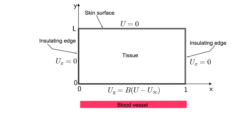
In this model, $U(x,y,t)$ is the local tissue temperature, $P_{f}(x,y)$ is the so-called blood perfusion coefficient, $G=G(x,y,t)$ is a source term which stands for metabolic and spatial heat generation, $B$ is the Biot number, $U_{\infty}$ is the environmental temperature and $U_{0}=U_{0}(x,y)$ denotes the initial temperature. The boundary conditions (34)-(37) include prescribed temperature in the upper skin surface (the boundary $y={\rm L}$), adiabatic conditions (in the boundaries $x=0$ and $x=1$) and convective heat transfer between the tissue and an adjoint large blood vessel (in the boundary $y=0$), as displayed in Fig. 1.

Figure 1: Domain for perfusion estimation.

The problem under consideration consists of estimating the perfusion coefficient $P_{f}$ using the bioheat model and input data in the form of temperature measurements. In the approach used here, the bioheat model is transformed into a time-dependent semi-discrete system of ordinary differential equations involving perfusion coefficient values as a set of unknown parameters, and the parameter estimation problem is solved through LMMSS together with some regularization technique to stabilize the iterates. For this we consider $(n+1)^{2}$ mesh points of the form $(x_{i},y_{j})$, the Chebyshev mesh, based on Gauss-Lobatto points

$$x_{i}=\frac{1}{2}\left[1-\cos\left(\frac{i\pi}{n}\right)\right]\quad\text{e}\quad y_{j}=\frac{1}{2}\left[1-\cos\left(\frac{j\pi}{n}\right)\right],\quad i,j=0,\dots,n,$$

and we use the Chebyshev pseudospectral method (CPM) to discretize spatial derivatives. This yields the semi-discrete model,

$$\left\{\begin{array}[]{l}{\sf U}^{\prime}(t)={\sf A({\bf p})}{\sf U}(t)+{\sf S}(t),\;\;t>0\\ {\sf U}(0)=U_{0},\end{array}\right.$$ (39)

where ${\bf p}$ is a vector that contains values of the perfusion coefficient along the mesh, ${\sf A}({\bf p})$ is a square matrix that depends on ${\bf p}$ and ${\sf S}(t)$ is a vector valued function that incorporates information about the source term $G$ and boundary conditions. The reconstruction of the perfusion coefficient will be made pointwise by solving a nonlinear least squares problem with objective function

$$\phi(\textbf{p})=\frac{1}{2}\|{\sf U}(\textbf{p})-\widetilde{\sf U}\|_{2}^{2}\doteq\dfrac{1}{2}\sum_{k=1}^{N}\sum_{\ell=1}^{M}\|U(\ell,t_{k},\textbf{{p}})-\widetilde{U}(\ell,t_{k})\|^{2},$$

where $U(\ell,t_{k},\textbf{{p}})$ denotes computed temperature values as functions of parameter p at prescribed locations inside the domain at time $t_{k}$, and $\widetilde{U}(\ell,t_{k})$ are measured temperature data at the same locations. As usually seen in inverse heat conduction problems, we will assume that available data and exact data satisfy

$$\widetilde{\sf U}={\sf U}+{\bf e},$$

where ${\sf U}$ contains temperature values calculated by a second order predictor-corrector method that combines a Runge-Kutta method as predictor and Crank-Nicolson method as corrector, and ${\sf e}$ is a vector representing inaccuracies. For a complete analysis on the discretization procedure of the bioheat model we refer the reader to Bazán et. al [4].

Jacobian matrices $J_{k}$ required along the minimization process are computed by solving the so-called sensitivity problem, where each column of $J_{k}$ comes from solving an initial value problem (IVP) very similar to (39) involving highly sparse matrices [4]. Moreover, since the nonhomogeneous terms for all IVPs are linearly independent, see [11, Section 3.1], it can be proved that the Jacobian is full column rank. Thus, irrespective of the chosen scaling matrix $L$, the assumption ${\cal N}(J_{k})\cap{\cal N}(L)=\{\bf 0\}$ is satisfied and hence the LMMSS iterates are well defined.

As for the scaling matrix, we choose $L={\cal L}_{i}$, with

$$\mathcal{L}_{i}=\left[\begin{array}[]{c}I_{n}\otimes L_{i}(n+1)\\ L_{i}(n)\otimes I_{n+1}\end{array}\right],\quad i=1,2,3,$$ (40)

where $\otimes$ represents the Kronecker product (or tensor product),

$$\small L_{1}(n) =\left[\begin{array}[]{cccc}-1&1&&\\ &\ddots&\ddots&\\ &&-1&1\end{array}\right]\in\mathbb{R}^{(n-1)\times n},$$

$$L_{2}(n) =\left[\begin{array}[]{ccccc}1&-2&1&&\\ &\ddots&\ddots&\ddots&\\ &&1&-2&1\end{array}\right]\in\mathbb{R}^{(n-2)\times n},$$

$$L_{3}(n) =\left[\begin{array}[]{ccccccc}-1&3&-3&1&&&\\ &-1&3&-3&1&&\\ &&\ddots&\ddots&\ddots&\ddots&\\ &&&-1&3&-3&1\\ \end{array}\right]\in\mathbb{R}^{(n-3)\times n},$$

with $L_{1}$, $L_{2}$ and $L_{3}$ representing discrete versions of the first, second and third order derivative operators, respectively, widely used, for example, in image reconstruction problems and other applications [5, 4, 22]. By the way, ${\cal L}_{i}$ is singular as

$${\cal N}(L_{1}(n)) =\text{span}\{[1,1,\dots,1]^{T}\},$$

$${\cal N}(L_{2}(n)) =\text{span}\{[1,1,\dots,1]^{T},[1,2,\dots,n]^{T}\},$$

$${\cal N}(L_{3}(n)) =\text{span}\{[1,1,\dots,1]^{T},[1,2,\dots,n]^{T},[1^{2},2^{2},\dots,n^{2}]^{T}\}.$$

The purpose of considering these 2D derivative operators into the numerical treatment of this inverse problem is to illustrate the impact of them on the numerical reconstruction when the exact solution is known to be smooth. In order to proceed, observe that the estimation problem involves $(n+1)\times n$ unknowns. Here we consider $n=14$ (which means we deal with an optimization problem involving 210 unknowns), $M=63$ measurements at internal locations of the domain and $N=8$ time levels. Doing so, the Jacobian $J_{k}$ is of order $504\times 210$; for details about the choice of measurement temperature locations the reader is referred to Bazán et. al [4].

In what follows, to illustrate the impact that the regularizer choice causes on the quality of the reconstructions from noisy data, we will conduct several numerical experiments intended to estimate the perfusion coefficient of a bioheat model with exact solution given by

$$U(x,y,t)=\frac{e^{-\pi^{2}t}}{2(B+{\rm L})}[((B+{\rm L})y^{2}-By-{\rm L})\cos(\pi x)]+\frac{BU_{\infty}}{B+{\rm L}}({\rm L}-y),$$ (41)

for $B=0.015,\;U_{\infty}=0.001,\;{\rm L}=1,$ and exact smooth perfusion coefficient

$$P_{f}(x,y)=\sin(\pi xy).$$ (42)

To this end we use temperature measurements with the noise vector e containing zero mean Gaussian random numbers scaled so that $\|{\bf e}\|/\|{\sf U}\|=\|{\sf U}-\widetilde{\sf U}\|/\|{\sf U}\|={\rm NL}$, where NL denotes the noise level in the data, and conduct the reconstruction process for several values of NL.

It is worth mentioning that when solving inverse problems through iterative methods, it is of fundamental importance to stop the iterations before the noise in the data starts to deteriorate their quality. We achieved this objective through the discrepancy principle [34]: LMMSS iterations stop at the first index $j$ such that

$$\|{\sf U}({\bf p}^{(j)})-\widetilde{\sf U}\|\leq\tau\|{\bf e}\|,$$ (43)

where $\tau\geq 1$ is a safeguard parameter. For our numerical experiments we take $\tau=1.05$, a slightly tight parameter as measure of good fit between the continuous problem and the discretization.

In order to assess the accuracy of recovered quantities, we use the relative error

$${\rm RE}({\bf p}^{(j)})=\|{\bf p}^{(j)}-{\bf p}\|/\|{\bf p}\|$$

along interior points of the mesh, and the temperature reconstruction error defined by

$${\rm TRE}=\|{\sf U}({\bf p}^{(j)})-{\sf U}\|/\|{\sf U}\|.$$

We report in Table 1 numerical results obtained with LMMSS using the singular scaling matrices ${\cal L}_{i}$ from (40), including the case $L=I$, for ${\rm NL}=0.0001$ and ${\rm NL}=0.001$.

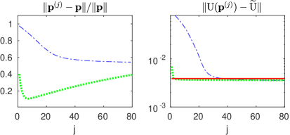
Before commenting on them, let us highlight Figure 2 where we monitor the relative error and absolute temperature error (which is proportional to the square root of the objective function) along the iterations of LMMSS with two different choices of $L$. While the plot on the right shows a monotone decay of objective function (residual norms), which is in accordance with the theoretical properties of LMMSS, on the left we see that, for $L={\cal L}_{2}$ (green curve), the relative error in the iterates ${\bf p}^{(j)}$ tends to deteriorate after the discrepancy principle is achieved (the threshold is represented by the red horizontal line) whereas for $L=I_{n}$ (blue curve) it seems to stabilize, but in a higher level. Concerning the residual norm (right) we observe that stopping criterion (43) is reached earlier for $L={\cal L}_{2}$.

Figure 2: Relative error ${\rm RE}({\bf p}^{(j)})$ (left) and absolute temperature error (right) as functions of the iteration number, from data with ${\rm NL}=0.001$. The blue dashed line corresponds to $L=I_{n}$ and the green dotted line to $L={\cal L}_{2}$. The horizontal red line on the right represents the value $\tau\|{\bf e}\|=0.0039.$

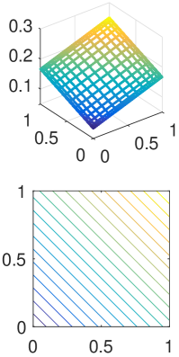
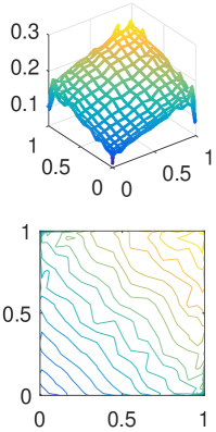
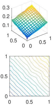
As for the quality of the reconstruction of the perfusion coefficient measured by the relative errors in Table 1, we note that it ranges from acceptable to excellent when $L={\cal L}_{i}$, $i=1,2,3$, which is also illustrated in Figure 3 where we present surface plots of the reconstructions. Notice that this fact should not be seen as a surprise, since the sought solution is smooth. Also note that the results obtained with classic LMM (Algorithm 1 using $L^{T}L=I_{n}$) are inferior both in terms of the quality of the reconstruction and the iterations count when compared to the other cases. Other than that, what really surprises is the superior quality of the reconstructed temperature compared to the quality of the reconstructed perfusion coefficient. Indeed, the occurrence of small temperature reconstruction errors (TREs) simply highlight the ill-posed nature of the problem. That is, the estimation problem allows for small temperature reconstruction errors in all cases, even with estimates of the perfusion coefficient differing greatly from the exact one.

Table 1: Results for perfusion coefficient recovery for two noise levels and $n+1=15$.

NL	Method	$L$	${\rm RE}({\bf p}^{(j)})$	TRE	Iterations
0.001	LMM	$I$	0.5860	4.0578e-04	36
	LMMSS	${\cal L}_{1}$	0.3437	3.0196e-04	6
	LMMSS	${\cal L}_{2}$	0.1718	2.3084e-04	3
	LMMSS	${\cal L}_{3}$	0.1403	2.3898e-04	2
0.0001	LMM	$I$	0.5333	5.4241e-04	44
	LMMSS	${\cal L}_{1}$	0.1539	3.7233e-05	7
	LMMSS	${\cal L}_{2}$	0.0990	3.1243e-05	4
	LMMSS	${\cal L}_{3}$	0.0516	2.6821e-05	3

Figure 3: Exact and recovered 2D perfusion coefficient. Noisy data correspond to $\textup{NL}=0.001$ (4 regularizers) and $\textup{NL}=0.0001$ only for ${\cal L}_{3}$ (last plot from left to right).

5.2 Reconstruction of thermal conductivity

In this section, we illustrate the effectiveness of LMMSS in a thermal conductivity reconstruction problem aiming at recovering the thermal conductivity incorporated as a parameter in a heat conduction model based on temperature measurements. For this we consider a two-dimensional heat conduction model in the finite domain $\Omega\times[0,t_{f}]$, $t_{f}>0$, with $\Omega=(0,l_{1})\times(0,l_{2})\subseteq\mathbb{R}^{2}$, $l_{1},l_{2}>0$, described by the partial differential equation (PDE)

$$C(x,y)\frac{\partial u}{\partial t}(x,y,t)=\nabla\cdot[{K}(x,y)\nabla u(x,y,t)]-q(x,y)u(x,y,t)+g(x,y,t),$$ (44)

boundary conditions

$$-k_{11}(0,y)\frac{\partial u}{\partial x}(0,y,t)+h_{1}(y)(u(0,y,t)-f_{1}(y,t))=0, \quad\text{on}\quad x=0,\ y\in(0,l_{2}),$$ (45)

$$k_{11}(l_{1},y)\frac{\partial u}{\partial x}(l_{1},y,t)+h_{2}(y)(u(l_{1},y,t)-f_{2}(y,t))=0, \quad\text{on}\quad x=l_{1},\ y\in(0,l_{2}),$$ (46)

$$-k_{22}(x,0)\frac{\partial u}{\partial y}(x,0,t)+h_{3}(x)(u(x,0,t)-f_{3}(x,t))=0, \quad\text{on}\quad y=0,\ x\in(0,l_{1}),$$ (47)

$$k_{22}(x,l_{2})\frac{\partial u}{\partial y}(x,l_{2},t)+h_{4}(x)(u(x,l_{2},t)-f_{4}(x,t))=0, \quad\text{on}\quad y=l_{2},\ x\in(0,l_{1}),$$ (48)

for all $t\in(0,t_{f}]$, and initial condition

$$u(x,y,0)=u_{0}(x,y)\quad\text{on}\ \Omega,$$ (49)

where $h_{i}$, $i=1,\dots,4$, are known as heat transfer functions, $f_{i}$, $i=1,\dots,4$, heat flux functions and $u_{0}(x,y)$ is the initial temperature distribution. The other variables stand for heat capacity $C(x,y)>0$, reaction term $q(x,y)\geq 0$, source term $g(x,y,t)$, temperature values $u(x,y,t)$ and thermal conductivity

$${K}(x,y)=\left[\begin{array}[]{cc}k_{11}(x,y)&0\\ 0&k_{22}(x,y)\end{array}\right],$$ (50)

where $k_{11}$ and $k_{22}$ are positive continuous functions.

In the direct problem associated with the heat conduction model described above, given the thermal conductivity $K$ and the other physical parameters, the goal is to determine the temperature $u(x,y,t)$. As for the recovery problem, it can be stated as follows: given a set of temperature measurements inside the spatial domain, we want to recover estimates of the parameter $K$ considering the other parameters involved in the model as input data. For a wide range of applications of the conductivity recovery problem on industry and engineering the reader is referred to [1, 3, 29, 24, 38, 2].

Clearly, since $K$ depends nonlinearly on $u$, what we face is a nonlinear inverse problem. Several parameter estimation methods which combine numerical methods for PDEs such as the finite difference method (FDM), the finite element method (FEM) or the boundary element method (BEM), and optimization techniques have been developed to address the conductivity estimation problem, e.g. [32, 30, 40, 1, 13]. In all cases the direct problem must be solved many times and therefore choosing a method to solve PDEs is crucial. The conductivity recovery method that we will illustrate in this section follows this line of action. In fact, it combines an efficient method to solve the direct problem (44)–(49) based on the Chebyshev pseudospectral method together with the Crank-Nicolson (CN) method as time integrator, and LMMSS as optimization tool for estimating the desired parameter. Our decision to choose such a PDE solver is supported by the fact that the former is is know to produce highly accurate approximations of spatial derivatives [11, 12], while the latter is second order accurate and absolutely stable [14].

As in the previous application, we consider $(n+1)^{2}$ mesh points based on Gauss-Lobatto points and use CPM to discretize spatial derivatives on $\Omega$. This transforms model (44)–(49) into a time-dependent system of ordinary differential equations (ODEs), the semi-discrete model,

$$\left\{\begin{aligned} &\textbf{C}\textbf{v}^{\prime}(t)=\textbf{Av}(t)+\textbf{S}(t),\ t>0\\ &\textbf{v}(0)=\textbf{u}^{0}\end{aligned}\right.,$$ (51)

where, roughly speaking, $\bf A$ contains spatial discretization terms involving conductivity values $K(x_{i},y_{j})$, $\bf S$ contains terms coming from the source $g$ and boundary information, $\bf C$ contains discrete heat capacity values, and $\textbf{u}^{0}$ consists of initial temperature values. Then, in order to determine temperature values at several time steps we use the Crank-Nicolson method.

As for the inverse problem, it is formulated as a nonlinear least squares problem involving temperature measurements as input data, usually contaminated with errors caused by imprecision in physical experiments or by external noise. The functional to be minimized is described by

$$\phi(\textbf{k})=\frac{1}{2}\|{\sf u}(\textbf{k})-\widetilde{\sf u}\|_{2}^{2}\doteq\dfrac{1}{2}\sum_{k=1}^{N}\sum_{j=0}^{n}\sum_{i=0}^{n}\|u(x_{i},y_{j},t_{k},\textbf{{k}})-\widetilde{u}(x_{i},y_{j},t_{k})\|^{2},$$

where

$$\textbf{k}=\left[\begin{array}[]{c}\textbf{k}_{11}\\ \textbf{k}_{22}\end{array}\right]\in\mathbb{R}^{2(n+1)^{2}}$$

contains unknowns $k_{11}(x_{i},y_{j})$ and $k_{22}(x_{i},y_{j})$ along the mesh points $(x_{i},y_{j})$, ${\sf u}(\textbf{k})$ denotes an $[(n+1)^{2}N]\times 1$ block vector containing solutions of the direct problem for given ${\bf k}$, with the $k$-th block being associated with time level $t_{k}$, $k=1,\dots,N$, and $\widetilde{\sf u}$ is a vector of measured temperature data at the $N$ time steps with the same structure as ${\sf u}(\textbf{k})$. Jacobian matrices $J_{k}$ required along the minimization process are computed, as in the previous subsection, by solving the sensitivity problem. For details the reader is referred to [12, Sections 3.1 and 4] and [11, Section 3.1].

Here, we choose scaling matrices $L=\tilde{\cal L}_{i}$,

$$\tilde{\cal L}_{i}=\left[\begin{array}[]{c}I_{n+1}\otimes L_{i}(n+1)\\ L_{i}(n+1)\otimes I_{n+1}\end{array}\right],\quad i=1,2.$$ (52)

which differs slightly from that used in the previous application (see (40)) because of the boundary conditions, but following the same ideas.

As in the previous example, we will assume that the received data $\widetilde{\sf u}$ and the exact data ${\sf u}$ satisfy

$$\widetilde{\sf u}={\sf u}+{\sf e},$$

where ${\sf e}$ contains zero mean Gaussian random numbers scaled so that $\|\widetilde{\sf u}-{\sf u}\|_{2}/\|\sf u\|_{2}=\textup{NL}$, where NL denotes the noise level. In the case of $\textup{NL}=0$, we stop the iterations at ${\bf k}^{(j)}$ if the gradient of the objective function is small, i.e.,

$$\|\nabla\phi({\bf k}^{(j)})\|_{2}<\varepsilon,$$

or if the relative variation of the iterates is small,

$$\frac{\|{\bf k}^{(j)}-{\bf k}^{(j-1)}\|_{2}}{\|{\bf k}^{(j)}\|_{2}}<\varepsilon,$$

both with $\varepsilon=5\times 10^{-4}$ in all numerical examples. Otherwise, if $\textup{NL}\neq 0$, the iterations stop using the discrepancy principle [34] as in (43) for $\tau=1.1$ in the numerical experiments of this section.

In the next subsections we will discuss examples and compare results obtained with classic LMM and LMMSS using data with and without noise. The accuracy of recovered conductivities is measured by relative errors,

$${\rm RE}({\bf k}_{11}^{(j)})=\|{\bf k}_{11}^{(j)}-{\bf k}_{11}\|_{2}/\|{\bf k}_{11}\|_{2}\quad\text{and}\quad{\rm RE}({\bf k}_{22}^{(j)})=\|{\bf k}_{22}^{(j)}-{\bf k}_{22}\|_{2}/\|{\bf k}_{22}\|_{2},$$

as well as by temperature reconstruction errors TRE defined similarly as in the perfusion estimation problem.

To rigorously evaluate the results obtained in the numerical simulations, two test problems will be solved 30 times using different noisy temperature data. We will report average relative errors of reconstructed quantities, including the maximum number of iterations of all instances, denoted by MI, spent until some convergence criterion is met. In both examples we consider $N=10$ equally spaced time stages in $[0,t_{f}]$ and $n+1=16$ grid points in each direction, which brings 256 conductivity unknowns $K(x_{i},y_{j})$ on $\Omega$.

5.2.1 Example 1: isotropic conductivity

Extracted from Mahmood and Lesnic [30], this example considers as sought solution $K(x,y)$ an isotropic conductivity, that is,

$$k_{11}(x,y)=k_{22}(x,y):=k(x,y)=\dfrac{1+x+y}{12},$$

the problem being defined on $\Omega=(0,1)\times(0,1)$, with final time $t_{f}=1$. The remaining parameters are:

$$C(x,y)=1,\quad g(x,y,t)=0,\quad f_{1}(y,t)=-1,\quad f_{2}(y,t)=1,$$

$$f_{3}(x,t)=-1,\quad f_{4}(x,t)=1,\quad\text{and}\quad h_{i}\equiv 0,\ i=1,\dots,4,$$

and initial condition $u_{0}(x,y)=0$. For this test problem the exact solution $u(x,y,t)$ is not available and temperature data for testing LMMSS should be generated artificially. We make this by applying a finite element method (FEM) to the model (44)–(49), using a refined mesh so as to build a highly accurate approximate solution $u$, which is then interpolated to the Chebyshev mesh to generate the sought “exact” solution. For more details on this procedure, see [12, Section 3.2].

Numerical results obtained from data with $\textup{NL}=0.001$ (i.e. data with relative noise level 0.1%), scaling matrices $L=I$ and $L=\tilde{\cal L}_{i}$ as in (52) are shown in Table 2 and Figure 4d. In all cases, for the initial guess we choose $k^{0}(x,y)=1/4$. As it can be seen, both scaling matrices used in this experiment yield good quality reconstructions, with reconstruction errors that do not exceed 10% of relative error but with an advantage in favor of LMMSS in terms of accuracy and computational effort.

Table 2: Results of one instance for different scaling matrices.

Scaling matrix	$I$	$\tilde{\mathcal{L}}_{1}$	$\tilde{\mathcal{L}}_{2}$
${\rm RE}({\bf k}^{(j)})$	0.0946	0.0128	0.0134
MI	7	4	4

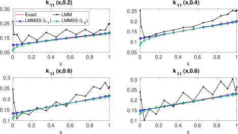
Also note the visual cohesion and smoothness displayed in in Figures 4c and 4d (effect of the derivative operator), contrasting with the presence of “peaks” in the reconstruction obtained with $L=I$ (classic LMM) displayed in Figure 4b .

Figure 4: Comparison between iterates generated by LMM and LMMSS.

(a) Exact

(b) $L=I$

(c) $L=\tilde{\mathcal{L}}_{1}$

(d) $L=\tilde{\mathcal{L}}_{2}$

5.2.2 Example 2: orthotropic conductivity

This example is taken from the work of Cao, Lesnic and Colaço [13], adapted to model (44)–(49), defined in $\Omega=(0,1)\times(0,1)$ and with final time $t_{f}=1$. In this case the exact solution of the model is available and defined as

$$u(x,y,t)=e^{-t}(\sin(\pi x)\sin(\pi y)+(\pi+1)(x+y)+1),$$

and the other model parameters are given as $h_{i}=1,\ i=1,\dots,4$, $C(x,y)=1$, $q(x,y)=0$,

$$f_{1}(y,t) =-\frac{1+y}{12}e^{-t}(\pi\sin(\pi y)+\pi+1)+e^{-t}((\pi+1)y+1),$$

$$f_{2}(y,t) =\frac{2+y}{12}e^{-t}(-\pi\sin(\pi y)+\pi+1)$$

$$\quad+e^{-t}(-\sin(\pi y)+(\pi+1)(1+y)+1),$$

$$f_{3}(x,t) =-\frac{1+0.5x}{12}e^{-t}(\pi\sin(\pi x)+\pi+1)+e^{-t}((\pi+1)x+1),$$

$$f_{4}(x,t) =\frac{2+0.5x}{12}e^{-t}(-\pi\sin(\pi x)+\pi+1)$$

$$\quad+e^{-t}(-\sin(\pi x)+(\pi+1)(1+x)+1),$$

source term

$$g(x,y,t) =-e^{-t}(\sin(\pi x)\sin(\pi y)+(\pi+1)(x+y)+1)$$

$$\quad-\frac{e^{-t}}{12}[2\pi+2+\pi\sin(\pi(x+y))]$$

$$\quad+\frac{\pi^{2}e^{-t}}{12}(2+1.5x+2y)\sin(\pi x)\sin(\pi y)$$

and, orthotropic conductivities

$$k_{11}(x,y)=\frac{1+x+y}{12}\quad\text{and}\quad k_{22}(x,y)=\frac{1+0.5x+y}{12}.$$ (53)

For this test problem, the iterates start with $k^{0}_{11}(x,y)=k^{0}_{22}(x,y)=1/4$ and the reconstruction problem is addressed for $\textup{NL}=0$, $\textup{NL}=0.001$ and $\textup{NL}=0.01$. As we are dealing with an orthotropic conductivity, the scaling matrices come in the form

$$L=I_{2}\otimes\tilde{\mathcal{L}}_{i},\quad i=1,2,$$

to ensure the smoothing effect of $\tilde{\mathcal{L}}_{i}$ on both $k_{11}$ and $k_{22}$ [11].

Average results are displayed in Table 3. From the table it is apparent that LMM does not produce good quality results with respect to relative errors to the exact solution, even in the case of noiseless data, which contrasts with the reconstructions obtained by the proposed method, with relative errors varying between 2% and 11% for $\textup{NL}=0.001$, and between 3% and 20% for $\textup{NL}=0.01$, which is very reasonable mainly for we deal with the numerical treatment of a nonlinear ill-posed problem from noisy data. Here it is worth noting that despite the quality of the reconstructions being very different, the same does not happen with the temperature reconstruction errors (TRE), which are small and close to each other for both methods. This is nothing more than the evidence that we are dealing with an ill-posed problem. In the noiseless case this also indicates the sum-of-squares function has more than one global minimizer ($X^{*}$ is not a singleton).

Table 3: Average results found for three noise levels.

NL	Method	$L$	${\rm RE}({\bf k}_{11}^{(j)})$	${\rm RE}({\bf k}_{22}^{(j)})$	TRE	MI
0	LMM	$I$	0.2937	0.3698	0.0000	13
	LMMSS	$I_{2}\otimes\tilde{\mathcal{L}}_{1}$	0.0195	0.0154	0.0000	6
	LMMSS	$I_{2}\otimes\tilde{\mathcal{L}}_{2}$	0.0291	0.0127	0.0000	8
0.001	LMM	$I$	0.3996	0.5211	0.0063	4
	LMMSS	$I_{2}\otimes\tilde{\mathcal{L}}_{1}$	0.0218	0.0185	0.0003	3
	LMMSS	$I_{2}\otimes\tilde{\mathcal{L}}_{2}$	0.0611	0.1138	0.0100	2
0.01	LMM	$I$	0.5100	0.6851	0.0398	1
	LMMSS	$I_{2}\otimes\tilde{\mathcal{L}}_{1}$	0.0388	0.0318	0.0022	2
	LMMSS	$I_{2}\otimes\tilde{\mathcal{L}}_{2}$	0.1446	0.2024	0.0237	1

Figure 5 presents the average results obtained for $k_{11}$ for different $y$ values and $\textup{NL}=0.001$. Once more it can be seen that while LMMSS produces solutions of good quality, LMM brings solutions with high oscillations and reconstructions far from the desired. Similar results were found for $k_{22}$. Here it is worth noting that among the scaling matrices tested in this simulation, $L=I_{2}\otimes\tilde{\mathcal{L}}_{1}$ was the one that produced the best results. We believe that this is due to the fact that as the solution is linear, a second order derivative operator would tend to diminish the importance of the term $\|L{\bf k}\|$ in the minimization process.

Figure 5: Average results for $k_{11}(x,y)$ for some fixed $y$ values and $\textup{NL}=0.001$. In the legends, $L_{1}$ and $L_{2}$ represent, respectively, $I_{2}\otimes\tilde{\mathcal{L}}_{1}$ and $I_{2}\otimes\tilde{\mathcal{L}}_{2}$.

6 Conclusion

Motivated by the improved performance of the Tikhonov regularization method in general form when solving discrete ill-posed problems with smooth solution [20], we proposed a version of the Levenberg-Marquardt method with singular scaling matrix which we named LMMSS. Under a completeness condition often used in the analysis of linear ill-posed problems we showed that the LMMSS iterates are well defined and establish that it has local quadratic convergence under an error bound assumption for the zero residue case. We also prove that the search directions $d_{k}$ are gradient-related and with that we ensure that the limit points of the sequence generated by LMMSS are stationary points of the sum-of-squares function.

As potential applications, we study two parameter identification problems involving a 2D heat conduction models. Since in these applications the parameter to be identified is supposed to be smooth, in LMMSS we introduce singular scaling matrices chosen as discrete derivative operators aiming to promote smoothness in the reconstructed parameter. To mitigate the effect of inaccuracies in the data, the discrepancy principle is used as stopping criterion. Numerical results using synthetic data illustrate that LMMSS can be useful in practical applications, mainly due to the high quality of the reconstructions and the low operational cost. However, continued experience with LMMSS in other applications is necessary to fully assess its potential.

For now, our convergence analysis only covers the case where $L$ is fixed through the iterations. This is in line with some applications, in which the proposal is to introduce desired properties present (or expected) in the exact solution. In such scenario, matrix $L$ does not need to change in each iteration. Nevertheless, it should be interesting in other applications to consider an iteration-dependent $L_{k}$. The convergence analysis in this case shall be subject of a future investigation.

Another future objective is to address the local convergence of LMM with singular scaling in the context of nonzero-residue problems by extending the results in [7].

Besides, in order to consider large-scale problems, strategies for exploiting sparsity and special structure for solving the LMM linear system as well as inexact solution of the LMM subproblem will also be considered in future works.

Appendix A Some technical proofs

Proof of Lemma 2.3.

Proof.

First, observe that, for any fixed $\lambda$, we have

$$\lim_{\gamma\rightarrow\infty}\psi(\gamma,\lambda)=1.$$ (54)

Now, given $\lambda>0$, observe that

$$\frac{\partial\psi}{\partial\gamma}(\gamma,\lambda)=\frac{(2\lambda-1)\gamma^{2}+\lambda}{\sqrt{1+\gamma^{2}}(\gamma^{2}+\lambda)^{2}}.$$ (55)

• Consider a fixed $\lambda\in(0,1/2)$. Since the maximizers of $\psi(\gamma,\lambda)$, for $\gamma>0$ must satisfy $\frac{\partial\psi}{\partial\gamma}(\gamma,\lambda)=0$, from (55), we have

  $$(2\lambda-1)\gamma^{2}+\lambda=0\quad\Rightarrow\quad\gamma_{\max}=\sqrt{-\frac{\lambda}{2\lambda-1}},$$

  Replacing $\gamma_{\max}$ at $\psi(\gamma,\lambda)$, we obtain

  $$\psi(\gamma_{\max},\lambda)=\frac{1}{2\sqrt{\lambda-\lambda^{2}}}.$$

  Furthermore, since $\frac{\partial\psi}{\partial\gamma}(\gamma,\lambda)<0$, for $\gamma\in(\gamma_{\max},+\infty)$ and $\frac{\partial\psi}{\partial\gamma}(\gamma,\lambda)>0$, for $\gamma\in(0,\gamma_{\max})$, with $\psi(0,\lambda)=0$, we conclude that $\gamma_{\max}$ is the unique maximizer.

• Now, for a fixed $\lambda\in[1/2,+\infty)$, in view of (55), it follows that $\frac{\partial\psi}{\partial\gamma}(\gamma,\lambda)>0$ for $\gamma\geq 0$. Hence, $\psi$ is increasing for $\gamma\in[0,+\infty)$, with $\psi(0,\lambda)=0$. Then, from (54), we conclude that $\psi(\gamma,\lambda)\leq 1$, for all $\gamma\geq 0$.

∎

References

- [1] G. Alessandrini, M. V. de Hoop, and R. Gaburro. Uniqueness for the electrostatic inverse boundary value problem with piecewise constant anisotropic conductivities. Inverse Problems, 33(12):125013, 2017.
- [2] O. M. Alifanov. Inverse heat transfer problems. Springer Science and Business Media, Berlin, 2012.
- [3] Y. Altintas. Manufacturing Automation. Cambridge University Press, New York, 2000.
- [4] F. S. V. Bazán, L. Bedin, and L. S. Borges. Space-dependent perfusion coefficient estimation in a 2d bioheat transfer problem. Computer Physics Communications, 214:18–30, 2017.
- [5] F. S. V. Bazán, M. C. C. Cunha, and L. S. Borges. Extension of GKB-FP algorithm to large-scale general-form Tikhonov regularization. Numerical Linear Algebra, 21(3):316–339, 2014.
- [6] R. Behling, Y. Bello-Cruz, and L.R. Santos. Infeasibility and error bound imply finite convergence of alternating projections. SIAM Journal on Optimization, 31:2863–2892, 2021.
- [7] R. Behling, D. S. Gonçalves, and S. A. Santos. Local convergence analysis of the Levenberg–Marquardt framework for nonzero-residue nonlinear least-squares problems under an error bound condition. Journal of Optimization Theory and Applications, 183:1099–1122, 2019.
- [8] E. H. Bergou, Y. Diouane, and V. Kungurtsev. Convergence and complexity analysis of a Levenberg–Marquardt algorithm for inverse problems. Journal of Optimization Theory and Applications, 2020.
- [9] D. P. Bertsekas. Nonlinear Programming. Athena Scientific, second edition, 1999.
- [10] A. Björck. Least squares methods. In P. G. Ciarlet and J. L. Lions, editors, Handbook of Numerical Analysis, Vol. I: Finite Difference Methods (Part I) - Solution of Equations in (Part I). Elsevier, 1990.
- [11] E. Boos, F. S. V. Bazán, and V. M. Luchesi. Thermal conductivity reconstruction method with application in a face milling operation. To be submitted.
- [12] E. Boos, V. M. Luchesi, and F. S. V. Bazán. Chebyshev pseudospectral method in the reconstruction of orthotropic conductivity. Inverse Problems in Science and Engineering, 29(1):1–31, 2020.
- [13] K. Cao, D. Lesnic, and M. J. Colaço. Determination of thermal conductivity of inhomogeneous orthotropic materials from temperature measurements. Inverse Problems in Science and Engineering, 27(10):1372–1398, 2019.
- [14] J. Crank and P. Nicolson. A practical method for numerical evaluation of solutions of partial differential equations of the heat-conduction type. Mathematical Proceedings of the Cambridge Philosophical Society, 43(1):50–67, 1947.
- [15] H. Dan, N. Yamashita, and M. Fukushima. Convergence properties of the inexact levenberg-marquardt method under local error bound conditions. Optimization Methods and Software, 17:605–626, 2002.
- [16] H. W. Engl, M. Hanke, and A. Neubauer. Regularization of Inverse Problems, volume 375 of Mathematics and its Applications. Kluwer Academic Publishers Group, Dordrecht, 1996.
- [17] J. Fan. A modified Levenberg-Marquardt algorithm for singular system of nonlinear equations. Journal of Computational Mathematics, 21(5):625–636, 2003.
- [18] J. Fan and Y. Yuan. On the quadratic convergence of the Levenberg-Marquardt method without nonsingularity assumption. Computing, 74(1):23–29, 2005.
- [19] R. Fletcher. A modified marquardt subroutine for non-linear least squares. Atomic Energy Research Establishment, pages 1–24, 1971.
- [20] P. C. Hansen. Rank-Deficient and Discrete Ill-Posed Problems. SIAM, Philadelphia, 1998.
- [21] P. C. Hansen. Discrete Inverse Problems - Insight and Algorithms. SIAM, Philadelphia, 2010.
- [22] P. C. Hansen, J. G.Nagy, and D. P. O’Leary. Deblurring Images - Matrices, Spectra and Filtering. SIAM, Philadelphia, 2006.
- [23] A. J. Hoffman. On approximate solutions of systems of linear inequalities. J. Nat. Bur. Stand., 49:263–265, 1952.
- [24] Z. Hou and R. Komanduri. General solutions for stationary/moving plane heat source problems in manufacturing and tribology. International Journal of Heat and Mass Transfer, 43:1679–1698, 2000.
- [25] Dennis Jr and J. R. Nonlinear least squares and equations. In D. Jacobs, editor, The State of the Art in Numerical Analysis. Academic Press, London, 1977.
- [26] Dennis Jr, J. R., and R. B. Schnabel. Numerical Methods for Unconstrained Optimization and Nonlinear Equations. SIAM, Philadelphia, 1996.
- [27] C. Kanzow, N. Yamashita, and M. Fukushima. Levenberg-Marquardt methods with strong local convergence properties for solving nonlinear equations with convex constraints. Journal of Computational and Applied Mathematics, 172(2):375–397, 2004.
- [28] K. Levenberg. A method for the solution of certain non-linear problems in least squares. Quarterly of Applied Mathematics, 2:164–168, 1944.
- [29] V. M. Luchesi and R. Coelho. An inverse method to estimate the moving heat source in machining process. Applied Thermal Engineering, 45:64–78, 2012.
- [30] M. S. Mahmood and D. Lesnic. Identification of conductivity in inhomogeneous orthotropic media. Int J Numer Method Heat Fluid Flow, 29(1):165–183, 2019.
- [31] Donald Marquardt. An algorithm for least-squares estimation of nonlinear parameters. SIAM Journal on Applied Mathematics, 11(2):431–441, 1963.
- [32] N. S. Mera, L. Elliott, D. B. Ingham, et al. An iterative BEM for the Cauchy steady state heat conduction problem in an anisotropic medium with unknown thermal conductivity tensor. Inverse Probl Eng, 8(6):579–607, 2000.
- [33] J. J. Moré. The Levenberg-Marquardt algorithm: Implementation and theory. In G. A. Watson, editor, Numerical Analysis volume 630 of Lecture Notes in Mathematics, pages 105–116. Springer Berlin Heidelberg, 1978.
- [34] V. A. Morozov. Methods for Solving Incorrectly Posed Problems. Springer-Verlag, New York, 1984.
- [35] W. Nowak and O. A. Cirpka. A modified Levenberg-Marquardt algorithm for quasi-linear geostatistical inversing. Advances in Water Resources, 27(7):737–750, 2004.
- [36] M. R. Osborne. Nonlinear least squares – The Levenberg algorithm revisited. J. Austral. Math. Soc., 19(3):343–357, 1976.
- [37] A. M. Ostrowski. A quantitative formulation of sylvester’s law of inertia. Proceedings of the National Academy of Sciences of the United States of America, 45(5):740–744, 1959.
- [38] M. N. Özişik. Heat Conduction. John Wiley & Sons, 2 edition, 1993.
- [39] C. C. Paige and M. A. Saunders. Towards a generalized singular value decomposition. SIAM J. Numer. Anal, 18:398–405, 1981.
- [40] J. Pasdunkorale and I. W. Turner. A second order finite volume technique for simulating transport in anisotropic media. Int J Numer Method Heat Fluid Flow, 13(1):31–56, 2003.
- [41] Harry H. Pennes. Analysis of tissue and arterial blood temperatures in the resting human forearm. Journal of Applied Physiology, 1(2):93–122, 1948.
- [42] S. M. Robinson. Some continuity properties of polyhedral multifunctions. Math. Programm. Study, 14:206–214, 1981.
- [43] H. Schwetlick and V. Tiller. Nonstandard scaling matrices for trust region gauss-newton methods. SIAM J. Sci. Stat. Comput., 10(4):654–670, 1989.
- [44] A. N. Tikhonov, A. V. Goncharsky, and Stepanov VV. Numerical methods for the solution of ill-posed problems, volume 328. Springer Science & Business Media, Dordrecht, 1 edition, 1995.
- [45] M. K. Transtrum and J. P. Sethna. Improvements to the Levenberg-Marquardt algorithm for nonlinear least-squares minimization, 2012. arXiv:1201.5885.
- [46] C. F. Van Loan. Generalizing the singular value decomposition. SIAM J. Numer. Anal, 13:76–83, 1976.
- [47] C. F. Van Loan. Computing the CS and the generalized singular value decompositions. Numer. Math., 46:479–491, 1985.
- [48] N. Yamashita and M. Fukushima. On the rate of convergence of the Levenberg-Marquardt method. In Topics in numerical analysis, pages 239–249. Springer, 2001.
- [49] G. Zhou and J. Si. Advanced neural-network training algorithm with reduced complexity based on jacobian deficiency. IEEE Transactions on Neural Networks, 9(3):448–453, 1998.