Bordered ${\mathit{HF}}^{-}$ for three-manifolds with torus boundary

Abstract.

We define an invariant for bordered 3-manifolds with torus boundary, taking the form of a module over a weighted $A$-infinity algebra associated to a torus defined in previous work. On setting $U=0$, we obtain the bordered three-manifold invariants with torus boundary constructed earlier.

1. Introduction

Heegaard Floer homology ${\mathbf{HF}}^{-}$ is a 3-manifold invariant [OSz04], which is a graded module over the ring of formal power series ${\mathbb{F}_{2}}[[U]]$. Its $U=0$ specialization is a somewhat simpler 3-manifold invariant, denoted $\widehat{\mathit{HF}}$. In [LOT18], we extended $\widehat{\mathit{HF}}$ to define bordered Floer homology, which associates

• a differential graded algebra $\mathcal{A}(F)$ to a closed, connected surface $F$;

• an $A_{\infty}$-module $\widehat{\mathit{CFA}}(Y_{1})$ over $\mathcal{A}(F)$ to a 3-manifold $Y_{1}$ equipped with an identification $\partial Y_{1}\cong F$; and

• a dg module (or type $D$ structure) $\widehat{\mathit{CFD}}(Y_{2})$ over $\mathcal{A}(F)$ to a 3-manifold $Y_{2}$ equipped with an identification $\partial Y_{2}\cong-F$.

A pairing theorem expresses as a (suitable) tensor product the invariant $\widehat{\mathit{HF}}$ for a $3$-manifold $Y$ that is divided into two pieces $Y_{1}$ and $Y_{2}$ along a connected surface $F$: if $\widehat{\mathit{CF}}(Y)$ denotes the chain complex whose homology is $\widehat{\mathit{HF}}(Y)$ then

$$\widehat{\mathit{CF}}(Y)\simeq\widehat{\mathit{CFA}}(Y_{1})\boxtimes\widehat{\mathit{CFD}}(Y_{2}).$$

Although $\widehat{\mathit{HF}}$ is adequate for many topological applications, the unspecialized version ${\mathbf{HF}}^{-}$ carries rich additional structure, making it, for example, the basic building block for the invariant of smooth, closed $4$-manifolds [OSz06].

In this paper, we construct a generalization of bordered Floer homology for 3-manifolds with torus boundary, with a view towards expressing the unspecialized Heegaard Floer homology ${\mathbf{HF}}^{-}(Y)$ for a $3$-manifold that is divided into two along a torus.

The general structure is as follows. Roughly, to $T^{2}$ we associate an algebra $\mathcal{A}_{-}=\mathcal{A}_{-}(T^{2})$. More precisely, $\mathcal{A}_{-}$ is a curved formal deformation of an $A_{\infty}$-algebra or what we call a weighted algebra. (See Section 1.1 or [LOT21].) To a 3-manifold $Y$ with boundary identified with $T^{2}$ we associate a (weighted) right $A_{\infty}$-module $\mathit{CFA}^{-}(Y)$ over $\mathcal{A}_{-}$, which is well-defined up to (weighted) homotopy equivalence. There is also a (weighted) type DD bimodule $\mathit{CFDD}^{-}(\mathbb{I})$ over $\mathcal{A}_{-}$ which is, at least philosophically, associated to the identity cobordism of $T^{2}$. In future work [LOT] we will establish a pairing theorem: if $\partial Y_{2}=T^{2}=-\partial Y_{1}$ then

$$\bigl{(}\mathit{CFA}^{-}_{U=1}(Y_{1})\otimes_{{\mathbb{F}_{2}}}\mathbf{CFA}^{-}(Y_{2})\bigr{)}\boxtimes_{\mathcal{A}_{-}^{U=1}\otimes\mathbfcal{A}_{-}}\mathit{CFDD}^{-}(\mathbb{I})\simeq\mathbf{CF}^{-}(Y_{1}\cup_{\partial}Y_{2}),$$

where $\boxtimes$ is an appropriate tensor product and $\mathbf{CFA}^{-}$ and $\mathbfcal{A}_{-}$ denote appropriate completions of $\mathit{CFA}^{-}$ and $\mathcal{A}_{-}$ (see Section 7.2). With a little further algebra (see Section 1.5 or [LOT20]), we can re-associate this tensor product as

$$\mathbf{CFA}^{-}(Y_{2})\boxtimes_{\mathbfcal{A}_{-}}(\mathit{CFA}^{-}_{U=1}(Y_{1})\boxtimes_{\mathcal{A}_{-}^{U=1}}\mathit{CFDD}^{-}(\mathbb{I}))$$

and so, if we define

$$\mathit{CFD}^{-}(Y_{1})=\mathit{CFA}^{-}_{U=1}(Y_{1})\boxtimes_{\mathcal{A}_{-}^{U=1}}\mathit{CFDD}^{-}(\mathbb{I})$$

then we recover the familiar-looking pairing theorem

$$\mathbf{CF}^{-}(Y_{1}\cup_{\partial}Y_{2})\simeq\mathbf{CFA}^{-}(Y_{2})\boxtimes_{\mathbfcal{A}_{-}}\mathit{CFD}^{-}(Y_{1}),$$

which is a strict generalization of the pairing theorem for $\widehat{\mathit{HF}}$ for $3$-manifolds glued along a torus boundary [LOT18].

This sketch hides some algebraic details about weighted algebras and modules, as well as the definitions of the invariants and proofs of the main results. We spell out some of these missing details presently and give references for some of the others.

Remark 1.1.

In [OSz04], ${\mathit{HF}}^{-}$ denoted a module defined over a polynomial ring ${\mathbb{F}_{2}}[U]$. The invariant ${\mathbf{HF}}^{-}$ we consider here is the completion of this module over the ring of power series ${\mathbb{F}_{2}}[[U]]$. With additional bookkeeping, one could work out the uncompleted theory; but we have not done so, in part because the current three-dimensional and four-dimensional applications of Heegaard Floer homology can be formulated in terms of the completed theory.

1.1. The torus algebra

The algebra $\mathcal{A}_{-}$ is studied in detail in our previous paper [LOT21]. We review aspects of the construction here.

1.1.1. Weighted algebras

A weighted $A_{\infty}$-algebra, or simply weighted algebra, over a commutative ring $\mathds{k}$ of characteristic $2$ is a curved $A_{\infty}$-algebra $\mathcal{A}$ over $\mathds{k}[[t]]$ together with an isomorphism of $\mathds{k}[[t]]$-bimodules $\mathcal{A}\cong A\otimes_{\mathds{k}}\mathds{k}[[t]]$ so that the curvature is contained in $tA$ [LOT20, Definition LABEL:Abs:def:wAinfty] (see also [LOT20, Remark LABEL:Abs:remark:weighted-is-deformation] and [LOT21, Definition LABEL:TA:def:weighted-alg]). Given a weighted $A_{\infty}$-algebra $\mathcal{A}$ we can extract operations

$$\mu_{n}^{w}\nobreak\mskip 2.0mu\mathpunct{}\nonscript\mkern-3.0mu{:}\penalty 300\mskip 6.0mu plus 1.0muA^{\otimes n}\to A$$

by

$$\mu_{n}=\sum_{w=0}^{\infty}\mu_{n}^{w}t^{w}.$$

(We are suppressing the grading shifts. A more precise version is given in Section 2.2; see especially Formula (2.1).) The condition that the curvature lies in $tA$ is equivalent to the condition that $\mu_{0}^{0}=0$. We will typically refer to $\mathcal{A}=(A,\{\mu_{n}^{w}\})$, not $(\mathcal{A},\{\mu_{n}\})$, as the weighted $A_{\infty}$-algebra. The condition that $(\mathcal{A},\{\mu_{n}\})$ is a curved $A_{\infty}$-algebra is equivalent to the condition that the $\mu_{n}^{w}$ satisfy the weighted $A_{\infty}$-relations

(1.2) $$\sum_{\begin{subarray}{c}1\leq i\leq j\leq n+1\\ w_{1}+w_{2}=w\end{subarray}}\mu^{w_{1}}_{n-j+i+1}(a_{1},\dots,a_{i-1},\mu_{j-i}^{w_{2}}(a_{i},\dots,a_{j-1}),a_{j},\dots,a_{n})=0,$$

for each $w\geq 0$ and $n\geq 0$.

A weighted $A_{\infty}$-algebra has an undeformed $A_{\infty}$-algebra $(A,\{\mu_{n}^{0}\})$, and an underlying $\mathds{k}$-bimodule $A$.

1.1.2. Building the algebra in three steps

We define the weighted algebra $\mathcal{A}_{-}$ associated to the torus in three steps:

1. There is an associative algebra $\mathcal{A}_{-}^{0,\mathrm{as}}$, which is the path algebra with relations:

   $$\vbox{\hbox{$\leavevmode\hbox to98.36pt{\vbox to59.45pt{\text{[drawing]}}}$}}/(\rho_{2}\rho_{1}=\rho_{3}\rho_{2}=\rho_{4}\rho_{3}=\rho_{1}\rho_{4}=0). \iota_{0} \iota_{1} \scriptstyle\rho_{1} \scriptstyle\rho_{2} \scriptstyle\rho_{3} \scriptstyle\rho_{4} \iota_{0} \iota_{1} \scriptstyle\rho_{1} \scriptstyle\rho_{2} \scriptstyle\rho_{3} \scriptstyle\rho_{4}$$

2. We define an $A_{\infty}$-algebra $\mathcal{A}_{-}^{0}$ which is a deformation of $\mathcal{A}_{-}^{0,\mathrm{as}}$. That is, as an ${\mathbb{F}_{2}}[U]$-module, $\mathcal{A}_{-}^{0}={\mathbb{F}_{2}}[U]\otimes_{{\mathbb{F}_{2}}}\mathcal{A}_{-}^{0,\mathrm{as}}$; $\mathcal{A}_{-}^{0}$ has trivial differential; and $\mu_{2}$ on $\mathcal{A}_{-}^{0}$ is induced by multiplication on $\mathcal{A}_{-}^{0,\mathrm{as}}$.

3. Finally, we define a weighted algebra $\mathcal{A}_{-}$ whose undeformed $A_{\infty}$-algebra is $\mathcal{A}_{-}^{0}$.

It is convenient to formulate $\mathcal{A}_{-}^{0}$ and $\mathcal{A}_{-}$ using its gradings. Gradings are specified in terms of a group law on $({\textstyle\frac{1}{2}}\mathbb{Z})\times\mathbb{Z}^{4}$, with multiplication specified by

$$(m;a,b,c,d)\cdot(m^{\prime};a^{\prime},b^{\prime},c^{\prime},d^{\prime})\\ =\left(m+m^{\prime}+{\textstyle\frac{1}{2}}\left|\begin{smallmatrix}a&b\\ a^{\prime}&b^{\prime}\end{smallmatrix}\right|+{\textstyle\frac{1}{2}}\left|\begin{smallmatrix}b&c\\ b^{\prime}&c^{\prime}\end{smallmatrix}\right|+{\textstyle\frac{1}{2}}\left|\begin{smallmatrix}c&d\\ c^{\prime}&d^{\prime}\end{smallmatrix}\right|+{\textstyle\frac{1}{2}}\left|\begin{smallmatrix}d&a\\ d^{\prime}&a^{\prime}\end{smallmatrix}\right|,a+a^{\prime},b+b^{\prime},c+c^{\prime},d+d^{\prime}\right).$$

Define

$$\operatorname{gr}^{\prime}(\rho_{1}) =(-{\textstyle\frac{1}{2}};1,0,0,0) \operatorname{gr}^{\prime}(\rho_{2}) =(-{\textstyle\frac{1}{2}};0,1,0,0)$$

$$\operatorname{gr}^{\prime}(\rho_{3}) =(-{\textstyle\frac{1}{2}};0,0,1,0) \operatorname{gr}^{\prime}(\rho_{4}) =(-{\textstyle\frac{1}{2}};0,0,0,1)$$

and let $G^{\prime}$ be the subgroup of $({\textstyle\frac{1}{2}}\mathbb{Z})\times\mathbb{Z}^{4}$ generated by $\operatorname{gr}^{\prime}(\rho_{1})$, $\operatorname{gr}^{\prime}(\rho_{2})$, $\operatorname{gr}^{\prime}(\rho_{3})$, $\operatorname{gr}^{\prime}(\rho_{4})$, and $\lambda=(1;0,0,0,0)$. These formulas determine a grading on $\mathcal{A}_{-}^{0,\mathrm{as}}$ by $G^{\prime}$.

The $A_{\infty}$-algebra $\mathcal{A}_{-}^{0}$ is uniquely characterized (up to isomorphism) by the following properties [LOT21, Theorem LABEL:TA:thm:UnDefAlg-unique]:

• $\mathcal{A}_{-}^{0}$ is an $A_{\infty}$-deformation of $\mathcal{A}_{-}^{0,\mathrm{as}}$,

• $\mathcal{A}_{-}^{0}$ is graded by $(G^{\prime},\lambda)$, and

• $\mu_{4}(\rho_{4},\rho_{3},\rho_{2},\rho_{1})=U\iota_{1}$.

The weighted algebra $\mathcal{A}_{-}$ is uniquely characterized (up to isomorphism) by the following properties [LOT21, Theorem LABEL:TA:thm:MAlg-unique]:

• The undeformed $A_{\infty}$-algebra of $\mathcal{A}_{-}$ is $\mathcal{A}_{-}^{0}$.

• $\mathcal{A}_{-}$ is $(G^{\prime},\lambda)$-graded, with respect to the weight grading $\lambda_{w}=(1;1,1,1,1)$, and

• $\mu^{1}_{0}=\rho_{1}\rho_{2}\rho_{3}\rho_{4}+\rho_{2}\rho_{3}\rho_{4}\rho_{1}+\rho_{3}\rho_{4}\rho_{1}\rho_{2}+\rho_{4}\rho_{1}\rho_{2}\rho_{3}$.

The ground ring for $\mathcal{A}_{-}$ is $\mathds{k}={\mathbb{F}_{2}}[U]\langle\iota_{0},\iota_{1}\rangle$.

Example 1.3.

The only term which can cancel $\mu_{2}^{0}(\mu_{4}^{0}(\rho_{4},\rho_{3},\rho_{2},\rho_{1}),\rho_{4})=U\rho_{4}$ in the $A_{\infty}$-relation is $\mu_{2}^{0}(\rho_{4},\mu_{4}^{0}(\rho_{3},\rho_{2},\rho_{1},\rho_{4}))=U\rho_{4}.$ Thus, $\mu_{4}^{0}(\rho_{3},\rho_{2},\rho_{1},\rho_{4})=U\iota_{0}.$ By a similar argument, $\mu_{4}^{0}(\rho_{2},\rho_{1},\rho_{4},\rho_{3})=U\iota_{1}$ and $\mu_{4}^{0}(\rho_{1},\rho_{4},\rho_{3},\rho_{2})=U\iota_{0}$.

Similarly, the $5$-input, weight $0$ $A_{\infty}$-relation with inputs $(\rho_{3},\rho_{4},\rho_{3},\rho_{2},\rho_{1})$ implies that $\mu_{4}^{0}(\rho_{3}\rho_{4},\rho_{3},\rho_{2},\rho_{1})=U\rho_{3}.$ Thus,

$$\mu_{4}^{0}(\mu_{4}^{0}(\rho_{3}\rho_{4},\rho_{3},\rho_{2},\rho_{1}),\rho_{2},\rho_{1},\rho_{4})=U^{2}\iota_{0},$$

and grading considerations imply that the only term that can cancel this one in the $7$-input, weight $0$ $A_{\infty}$-relation is

$$\mu_{6}^{0}(\rho_{3}\rho_{4},\rho_{3},\rho_{2},\mu_{2}(\rho_{1},\rho_{2}),\rho_{1},\rho_{4})=U^{2}\iota_{0}.$$

Following our previous paper [LOT21, Definition LABEL:TA:def:TilingPattern], we will sometimes refer to operations of the form $\mu_{n}^{w}(a_{1},\dots,a_{n})=U^{k}\iota_{\ell}$ as centered operations.

1.1.3. Relationship of the algebra to holomorphic curves

Let $\mathcal{Z}$ denote the genus $1$ pointed matched circle. Given a Reeb chord $\rho$ in $\mathcal{Z}$ (of any positive length) there is an associated algebra element $\rho\in\mathcal{A}_{-}$. (In [LOT18] this algebra element was denoted $a(\rho)$, but in this paper denoting it by $\rho$ will not cause confusion.)

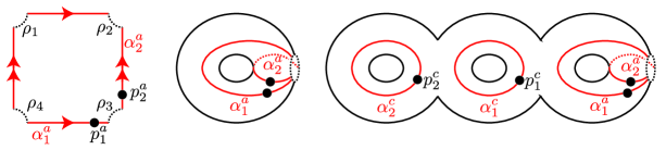
Figure 1. Some curves on punctured Riemann surfaces. Left and center: the case $g=1$. Right: the case $g=3$.

Fix $g\geq 1$ and let $\Sigma=\Sigma_{g}$ be a Riemann surface of genus $g$ with a single puncture, $\alpha_{1}^{a}$, $\alpha_{2}^{a}$ arcs in $\Sigma$ and $\alpha_{1}^{c},\dots,\alpha_{g-1}^{c}$ circles in $\Sigma$ as shown in Figure 1. Choose also a marked point $p^{a}_{i}$ on $\alpha_{i}^{a}$ and $p^{c}_{i}$ on $\alpha_{i}^{c}$. Note that $\mathcal{Z}$ is identified with $(\partial\Sigma,\partial(\alpha_{1}^{a}\cup\alpha_{2}^{a}))$. Let ${\boldsymbol{\alpha}}=\alpha_{1}^{a}\cup\alpha_{2}^{a}\cup\alpha_{1}^{c}\cup\dots\cup\alpha_{g-1}^{c}$.

Fix a non-negative integer $w$, a sequence of chords $\rho^{1},\dots,\rho^{n}$ in $\mathcal{Z}$ so that $\rho^{1}$ starts on $\alpha_{i}^{a}$, and a split complex structure $J=j_{\Sigma}\times j_{\mathbb{D}}$ on $\Sigma\times\mathbb{D}^{2}$. (We use superscripts in the list of Reeb chords because $\rho_{i}$ refers to a specific Reeb chord.) Let $\mathcal{N}([\alpha_{i}^{a}];\rho^{1},\dots,\rho^{n};w)$ denote the moduli space of $(j_{\Sigma}\times j_{\mathbb{D}})$-holomorphic maps

$$u\nobreak\mskip 2.0mu\mathpunct{}\nonscript\mkern-3.0mu{:}\penalty 300\mskip 6.0mu plus 1.0mu(S,\partial S)\to(\Sigma\times\mathbb{D}^{2},{\boldsymbol{\alpha}}\times S^{1}),$$

where $S$ is a surface with boundary, interior punctures, and boundary punctures, satisfying the following conditions:

1. The surface $S$ has exactly $n$ boundary punctures $q_{1},\dots,q_{n}$. Further, there are distinct points $\theta_{1},\dots,\theta_{n}\in(S^{1}\setminus\{1\})$, ordered counterclockwise around $\partial\mathbb{D}^{2}$ (starting at $1\in\partial\mathbb{D}^{2}$), so that at $q_{i}$, the map $u$ is asymptotic to $\rho^{i}\times\{\theta_{i}\}$. Moreover, all the $q_{i}$ lie on a single component of $\partial S$.

2. The surface $S$ has exactly $w$ interior punctures $r_{1},\dots,r_{w}$. Further, there are points $z_{1},\dots,z_{w}$ in the interior of $\mathbb{D}^{2}$ so that at $r_{i}$, $u$ is asymptotic to $S^{1}\times z_{i}$ (i.e., a simple orbit).

3. If $\overline{S}$ denotes the result of filling in the punctures of $S$, then the projection $\pi_{\mathbb{D}}\circ u$ extends to a $g$-fold branched cover $\overline{S}\to\mathbb{D}^{2}$.

4. The map $u$ passes through the points $(p^{c}_{1},1),\dots,(p^{c}_{g-1},1)$ and the point $(p^{a}_{i},1)$.

This space $\mathcal{N}$ is the moduli space of simple boundary degenerations; see Definitions 3.19 and 3.49. Its expected dimension $\operatorname{ind^{\square}}(\vec{\rho},w)$ is computed in Proposition 3.33; $\operatorname{ind^{\square}}(\vec{\rho},w)=2$ corresponds to the rigid moduli spaces.

We will show that, for appropriate choices of $j_{\Sigma}$, the moduli spaces $\mathcal{N}$ with $\operatorname{ind^{\square}}(\vec{\rho},w)\leq 2$ are transversely cut out and the number of points in them are, in fact, independent of $j_{\Sigma}$; this is part of Theorem 4.3 below.

We will often identify $\mathbb{D}^{2}\setminus\{1\}$ with a hyperbolic half-plane $\mathbb{H}$ presented as $(-\infty,1]\times\mathbb{R}\subset\mathbb{C}$. If $\overline{S}^{\prime}=\overline{S}\setminus(\pi_{\mathbb{D}}\circ u)^{-1}(1)$ then each component of $\partial\overline{S}^{\prime}$ is an arc $A$; and elementary complex analysis shows that $\pi_{\mathbb{H}}\circ u|_{A}\nobreak\mskip 2.0mu\mathpunct{}\nonscript\mkern-3.0mu{:}\penalty 300\mskip 6.0mu plus 1.0muA\to\{1\}\times\mathbb{R}$ is a monotone function. (This is an analogue of boundary monotonicity from [LOT18].)

Fix a point $z\in\Sigma\setminus{\boldsymbol{\alpha}}$. For any $u\in\mathcal{N}([\alpha_{i}^{a}];\rho^{1},\dots,\rho^{n};w)$, let $n_{z}(u)$ denote the local multiplicity of $\pi_{\mathbb{D}}\circ u$ at $z$. Since $\Sigma\setminus{\boldsymbol{\alpha}}$ is connected, $n_{z}(u)$ is independent of $z$. In fact, $n_{z}(u)$ is also independent of $u$: it depends only on $\rho^{1},\dots,\rho^{n}$ and $w$. (Specifically, $n_{z}(u)$ is $w$ plus the number of times $\rho_{4}$, or any other $\rho_{j}$, appears in the $\rho^{i}$.)

We can use these moduli spaces to define a weighted $A_{\infty}$-algebra:

Definition 1.4.

Let $\mathcal{A}_{-}^{0,\mathrm{as}}$ be as in Section 1.1.2. We define operations making ${\mathbb{F}_{2}}[U]\otimes_{{\mathbb{F}_{2}}}\mathcal{A}_{-}^{0,\mathrm{as}}$ into a weighted $A_{\infty}$-algebra $\mathcal{A}_{-}$ over ${\mathbb{F}_{2}}[U]$ as follows:

1. The operation $\mu_{1}^{0}$ vanishes, and the operation $\mu_{2}^{0}$ is inherited from $\mathcal{A}_{-}^{0}$.

2. The operation $\mu_{0}^{1}$ is $\rho_{1234}+\rho_{2341}+\rho_{3412}+\rho_{4123}$.

3. The centered operations (operations which output $U^{k}\iota_{i}$) are given by

   $$\mu_{n}^{w}(\rho^{1},\dots,\rho^{n})=\#\mathcal{N}([\alpha_{i}^{a}];\rho^{1},\dots,\rho^{n};w)U^{n_{z}(u)}\iota_{i}$$

   where $\iota_{i}$ is $\iota_{0}$ if $\rho^{1}$ starts on $\alpha_{1}$ and $\iota_{1}$ if $\rho^{1}$ starts on $\alpha_{2}$.

4. For each centered operation $\mu_{n}^{w}(\rho^{1},\dots,\rho^{n})=U^{m}\iota_{i}$ and any $\rho^{0}$ so that $\rho^{0}\rho^{1}\neq 0$, we have

   $$\mu_{n}^{w}(\rho^{0}\rho^{1},\dots,\rho^{n})=\rho^{0}\mu_{n}^{w}(\rho^{1},\dots,\rho^{n}).$$

   Similarly, for any $\rho^{n+1}$ so that $\rho^{n}\rho^{n+1}\neq 0$, we have

   $$\mu_{n}^{w}(\rho^{1},\dots,\rho^{n}\rho^{n+1})=\mu_{n}^{w}(\rho^{1},\dots,\rho^{n})\rho^{n+1}.$$

The above are the only nonzero operations of the form $\mu^{w}_{n}(\rho^{1},\dots,\rho^{n})$.

We can think of the non-centered operations as corresponding to holomorphic curves with two components, one of which is at $e\infty$; see Figure 2.

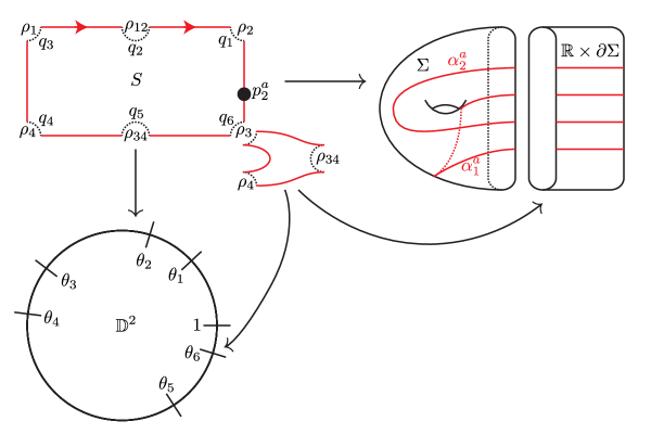
Figure 2. A schematic for a non-centered operation. The surface $S$ (top-left) maps to $\Sigma$ (top-right) times $\mathbb{D}^{2}$ (bottom-left). The component with punctures labeled $\rho_{3}$, $\rho_{4}$, and $\rho_{34}$ maps to $\mathbb{R}\times\partial\Sigma$ (east infinity) and the point $\theta_{6}$. This schematic corresponds to $\mu_{6}(\rho_{2},\rho_{12},\rho_{1},\rho_{4},\rho_{34},\rho_{34})=U^{2}\rho_{4}$.

If the Heegaard genus $g=1$, it is not hard to describe the spaces $\mathcal{N}([\alpha_{i}^{a}];\rho^{1},\dots,\rho^{n};w)$ combinatorially; see Section 4.2. Using this description, one can show that the operations $\mu_{n}^{w}$ define a weighted algebra in this case, and that algebra agrees with $\mathcal{A}_{-}$ from Section 1.1.2. (See Proposition 4.11.) Index computations and a degeneration argument then show that the counts of the spaces $\mathcal{N}([\alpha_{i}^{a}];\rho^{1},\dots,\rho^{n};w)$ are, in fact, independent of $g$ (and, as mentioned above, the complex structure). Together, this implies:

Theorem 1.5.

Definition 1.4 defines a weighted $A_{\infty}$-algebra that agrees with the weighted $A_{\infty}$-algebra defined in Section 1.1.2.

(This is proved in Section 4, as Theorem 4.3.)

1.2. The type A module

1.2.1. Weighted modules

Given a weighted $A_{\infty}$-algebra $\mathcal{A}$ over $\mathds{k}$, a weighted (right) $A_{\infty}$-module over $\mathcal{A}$ is a right $A_{\infty}$-module $\mathfrak{M}$ over $\mathcal{A}$ together with an isomorphism of $\mathds{k}[[t]]$-modules $\mathfrak{M}\cong M\otimes_{\mathds{k}}\mathds{k}[[t]]$. Like a weighted algebra, $M$ inherits operations

(1.6) $$m_{1+n}^{w}\nobreak\mskip 2.0mu\mathpunct{}\nonscript\mkern-3.0mu{:}\penalty 300\mskip 6.0mu plus 1.0muM\otimes_{\mathds{k}}\otimes\overbrace{A\otimes_{\mathds{k}}\dots\otimes_{\mathds{k}}A}^{k}\to M,$$

for $n,w\geq 0$, defined by

$$m_{1+k}=\sum m_{1+k}^{w}t^{w}.$$

(We will usually suppress the subscript $\mathds{k}$ from tensor products over the ground ring $\mathds{k}$ relevant at the time.) A weighted $A_{\infty}$-module is specified by the data $\mathfrak{M}=(M,\{m_{1+k}^{w}\})$. The curved $A_{\infty}$-relation turns into a compatibility condition for the $m_{1+k}^{w}$ similar to Formula (1.2) (see, e.g., [LOT20, Definition LABEL:Abs:def:wmod]).

Given weighted $A_{\infty}$-modules $\mathfrak{M}$ and $\mathfrak{N}$ over $\mathcal{A}$, there is a chain complex $\operatorname{Mor}_{\mathcal{A}}(\mathfrak{M},\mathfrak{N})$ of morphisms between them. The complex $\operatorname{Mor}_{\mathcal{A}}(\mathfrak{M},\mathfrak{N})$ is the complex of morphisms of $A_{\infty}$-modules over the curved $A_{\infty}$-algebra $\mathcal{A}$. Explicitly, an element is a sequence of maps

$$f_{1+n}^{w}\nobreak\mskip 2.0mu\mathpunct{}\nonscript\mkern-3.0mu{:}\penalty 300\mskip 6.0mu plus 1.0muM\otimes\overbrace{A\otimes\dots\otimes A}^{n}\to N$$

for $n,w\geq 0$, with differential given by the sum of all ways of pre-composing with an operation $\mu_{m}^{v}$ on $\mathcal{A}$ or $m_{1+m}^{v}$ on $\mathfrak{M}$ or post-composing by an operation $m_{1+m}^{v}$ on $\mathfrak{N}$. This makes the category of weighted $A_{\infty}$-modules over $\mathcal{A}$ into a dg category, and so it inherits the usual auxiliary notions of homomorphisms (cycles in the morphism complex), homotopic morphisms (morphisms whose difference is a boundary), and homotopy equivalences.

Remark 1.7.

The definition of a weighted $A_{\infty}$-module over $\mathcal{A}$ depends both on $\mathcal{A}$ and the ring $\mathds{k}$ that we are viewing $\mathcal{A}$ over: the operations $m_{1+n}^{w}$ in Formula (1.6) are $\mathds{k}$-equivariant. We will later construct two modules, $\mathit{CFA}^{-}$ and $\mathit{CFA}^{-}_{nu}$, which differ mainly in which ground ring they are defined over.

1.2.2. Unitality conditions

A weighted $A_{\infty}$-algebra $\mathcal{A}=(A,\{\mu_{n}^{w}\})$ is unital if there is an element $\mathbf{1}\in A$ so that $\mu^{0}_{2}(\mathbf{1},a)=\mu^{0}_{2}(a,\mathbf{1})=a$ for all $a\in A$ and $\mu^{w}_{n}(a_{1},\dots,a_{n})=0$ if $(w,n)\neq(0,2)$ and some $a_{i}=\mathbf{1}$.

Similarly, an $A_{\infty}$-module $\mathfrak{M}$ over a unital weighted $A_{\infty}$-algebra $\mathcal{A}$ is called unital if $m^{0}_{2}(\mathbf{x},\mathbf{1})=\mathbf{x}$ for all $\mathbf{x}\in M$, and

$$m^{w}_{n}(\mathbf{x},a_{1},\dots,a_{n-1})=0$$

if $(w,n)\neq(0,2)$ and some $a_{i}=\mathbf{1}$. Given two unital weighted $A_{\infty}$-modules $\mathfrak{M}$ and $\mathfrak{N}$ over a unital weighted $A_{\infty}$-algebra $\mathcal{A}$, there is a complex of unital morphisms between them, by requiring that each $f_{n}^{w}$ vanishes if some input is the unit $\mathbf{1}$. This gives rise to the notion of unital homotopy equivalences.

There are various other weaker notions of unitality one could work with (compare [LOT20, Section LABEL:Abs:subsec:UnitsHomPert]); the above version is sufficient for our purposes. The notion we are using here is referred to as strictly unital in our previous papers and some other parts of the literature.

1.2.3. Sketch of the definition of the type A module and statement of invariance

Fix a bordered Heegaard diagram (in the sense of [LOT18]) $\mathcal{H}=(\Sigma_{g},{\boldsymbol{\alpha}}^{a},{\boldsymbol{\alpha}}^{c},{\boldsymbol{\beta}},z)$ with $\partial\mathcal{H}$ the genus $1$ pointed matched circle, representing a bordered 3-manifold $(Y,\phi\nobreak\mskip 2.0mu\mathpunct{}\nonscript\mkern-3.0mu{:}\penalty 300\mskip 6.0mu plus 1.0muT^{2}\to\partial Y)$. Write ${\boldsymbol{\alpha}}={\boldsymbol{\alpha}}^{a}\cup{\boldsymbol{\alpha}}^{c}$. To this data we associate a right weighted $\mathcal{A}_{-}$-module $\mathit{CFA}^{-}(\mathcal{H})$ as follows. As a left ${\mathbb{F}_{2}}\langle\iota_{1},\iota_{2}\rangle[U]$-module, $\mathit{CFA}^{-}(\mathcal{H})$ is the same as ${\mathbb{F}_{2}}[U]\otimes_{\mathbb{F}_{2}}\widehat{\mathit{CFA}}(\mathcal{H})$, the free ${\mathbb{F}_{2}}[U]$-module generated by $g$-tuples $\mathbf{x}=\{x_{i}\}\subset({\boldsymbol{\alpha}}\cap{\boldsymbol{\beta}})$ with exactly one $x_{i}$ on each $\alpha$-circle and $\beta$-circle and at most one $x_{i}$ on each $\alpha$-arc, with the same action of the idempotents. The weighted operations are defined by counting pseudo-holomorphic curves.

Definition 1.8.

A basic algebra element is an element of the form

• $U^{m}\rho$ where $m\geq 0$ and $\rho$ is some Reeb chord (the Reeby elements) or

• $U^{m}\iota_{i}$ where $m>1$ and $\iota_{i}\in\{\iota_{0},\iota_{1}\}$ is one of the two basic idempotents.

Given a sequence $\vec{a}=(a_{1},\dots,a_{m})$ of basic algebra elements, if we set $U=1$ and drop all of the terms which are idempotents, we obtain a sequence of chords $\vec{\rho}=(\rho^{n_{1}},\dots,\rho^{n_{m}})$; we call this the underlying chord sequence of the sequence of basic algebra elements. That is, $\vec{\rho}$ has one term for each Reeby element in $\vec{a}$.

Given generators $\mathbf{x}$ and $\mathbf{y}$ for $\mathit{CFA}^{-}(\mathcal{H})$, an integer $w$, and a homotopy class $B\in\pi_{2}(\mathbf{x},\mathbf{y})$, let

$$\mathcal{M}^{B}(\mathbf{x},\mathbf{y};\vec{a};w)$$

denote the moduli space of embedded $J$-holomorphic maps

$$u\nobreak\mskip 2.0mu\mathpunct{}\nonscript\mkern-3.0mu{:}\penalty 300\mskip 6.0mu plus 1.0mu(S,\partial S)\to\bigl{(}\Sigma\times[0,1]\times\mathbb{R},({\boldsymbol{\alpha}}\times\{1\}\times\mathbb{R})\cup({\boldsymbol{\beta}}\times\{0\}\times\mathbb{R})\bigr{)}$$

asymptotic to $\mathbf{x}\times[0,1]\times\{-\infty\}$, $\mathbf{y}\times[0,1]\times\{+\infty\}$, and at $e\infty$ asymptotic to the chord sequence $\vec{\rho}$ and $w$ simple Reeb orbits. Curves in the moduli space are required to satisfy certain other technical conditions, analogous to [LOT18, Conditions (M-1)–(M-11)$\setminus$(M-9)]; (M-9) is omitted because curves here are allowed to cross the basepoint $z$. See Section 3.2. We are using the notation $J$ to indicate a family of almost complex structures on $\Sigma\times[0,1]\times\mathbb{R}$ depending on the sequence $\vec{a}$ and the locations in $[0,1]\times\mathbb{R}$ of the Reeb chords and orbits; this dependence is made precise in Definition 3.6, of a coherent family of almost complex structures. (The reason for using such families relates to transversality for boundary degenerations. In particular, the non-Reeby elements of $\vec{a}$ only affect the moduli space through the choice of $J$, not as asymptotics of the holomorphic curves $u$.) The integer $w$ is slightly redundant: it is determined by the data of $\vec{\rho}$ and $B$.

Let $\operatorname{ind}(B,\vec{a})$ denote the expected dimension of the moduli space $\mathcal{M}^{B}(\mathbf{x},\mathbf{y};\vec{a};w)$. Define a module $\mathit{CFA}^{-}_{nu}(\mathcal{H})$ which, as an ${\mathbb{F}_{2}}$-vector space, is the same as $\mathit{CFA}^{-}(\mathcal{H})$, i.e.,

$$\mathit{CFA}^{-}_{nu}(\mathcal{H})=\mathit{CFA}^{-}(\mathcal{H})={\mathbb{F}_{2}}[U]\otimes_{{\mathbb{F}_{2}}}\widehat{\mathit{CFA}}(\mathcal{H}).$$

Fix a suitably generic coherent family of almost complex structures $J$; we call such families tailored (Definition 3.51). Make $\mathit{CFA}^{-}_{nu}(\mathcal{H})$ into a weighted module over $\mathcal{A}_{-}$ with

$$m_{1+k}^{w}\nobreak\mskip 2.0mu\mathpunct{}\nonscript\mkern-3.0mu{:}\penalty 300\mskip 6.0mu plus 1.0mu\mathit{CFA}^{-}_{nu}(\mathcal{H})\otimes(\mathcal{A}_{-})^{\otimes k}\to\mathit{CFA}^{-}_{nu}(\mathcal{H})$$

given by

(1.9) $$m_{1+n}^{w}(\mathbf{x},a_{1},\dots,a_{n})=\sum_{\mathbf{y}}\sum_{\begin{subarray}{c}B\in\pi_{2}(\mathbf{x},\mathbf{y})\\ \operatorname{ind}(B,a_{1},\dots,a_{n})=1\end{subarray}}U^{m+n_{z}(B)}\cdot\#\mathcal{M}^{B}(\mathbf{x},\mathbf{y};a_{1},\dots,a_{n};w)\cdot\mathbf{y},$$

where $m$ is the total number of factors of $U$ in the $a_{1},\dots,a_{n}$. The conditions on the almost complex structures guarantee that these counts are finite (Lemma 3.60).

Remark 1.10.

This use of the term tailored for almost complex structures is unrelated to the use in the literature on embedded contact homology [CGHY].

Theorem 1.11.

Assuming that the bordered Heegaard diagram is provincially admissible and the family of almost complex structures $J$ is tailored, the operations $m_{1+k}^{w}$ give $\mathit{CFA}^{-}_{nu}$ the structure of a unital weighted $A_{\infty}$-module over $\mathcal{A}_{-}$ (with ground ring ${\mathbb{F}_{2}}\langle\iota_{1},\iota_{2}\rangle$).

The key step in the proof of Theorem 1.11 is the following analysis of the codimension-1 boundary of $\mathcal{M}^{B}(\mathbf{x},\mathbf{y};\vec{\rho};w)$:

Theorem 1.12.

Fix a provincially admissible bordered Heegaard diagram $\mathcal{H}$ and a tailored family of almost complex structures $J$ on $\Sigma\times[0,1]\times\mathbb{R}$. Given a homology class $B$ and sequence $\vec{a}=(a_{1},\dots,a_{k})$ of basic algebra elements so that $\operatorname{ind}(B;a_{1},\dots,a_{k};w)=2$, the sum of the following is $0\pmod{2}$:

1. The number of two-story holomorphic buildings, i.e.,

   $$\sum_{\begin{subarray}{c}\mathbf{x}^{\prime}\\ B_{1}+B_{2}=B\\ w_{1}+w_{2}=w\\ j=0,\dots,n\end{subarray}}\bigl{(}\#\mathcal{M}^{B_{1}}(\mathbf{x},\mathbf{x}^{\prime};a_{1},\dots,a_{j};w_{1})\bigr{)}\bigl{(}\#\mathcal{M}^{B_{2}}(\mathbf{x}^{\prime},\mathbf{y};a_{j+1},\dots,a_{n};w_{2})\bigr{)}.$$

2. The number of collisions of levels, i.e.,

   $$\sum_{a_{i}a_{i+1}\neq 0}\#\mathcal{M}^{B}(\mathbf{x},\mathbf{y};a_{1},\dots,a_{i}a_{i+1},\dots,a_{n};w)$$

3. The number of orbit curve degenerations, which corresponds to

   $$\sum_{i=0}^{n+1}\,\sum_{\begin{subarray}{c}\sigma\in\{\rho_{1234},\rho_{2341},\\ \rho_{3412},\rho_{4123}\}\end{subarray}}\#\mathcal{M}(\mathbf{x},\mathbf{y};a_{1},\dots,a_{i-1},\sigma,a_{i},\dots,a_{n};w-1).$$

4. If $\mathbf{x}=\mathbf{y}$, the number of simple boundary degeneration ends, which corresponds to

   $$U^{k}\#\mathcal{N}([\alpha_{i}^{a}];\vec{\rho};w),$$

   where $\alpha_{i}^{a}$ is the $\alpha$-arc containing an element of $\mathbf{x}$, $\vec{\rho}$ is the underlying chord sequence of $\vec{a}$, and $k$ is the sum of all the $U$-powers in the $a_{i}$; except that if any $a_{i}$ is of the form $U^{m}\iota_{j}$ then this count is defined to be zero.

5. The number of composite boundary degeneration ends, which corresponds to pairs $(u,v)$ where:

   • $u$ is an index one embedded curve in $\mathcal{M}^{B_{1}}(\mathbf{x},\mathbf{y},a_{1},\dots,a_{i-1},b,a_{j+1},\dots,a_{n};w_{1})$ for some $1\leq i<j\leq n$ and basic algebra element $b$;

   • $v\in\mathcal{N}(b;a_{i},\dots,a_{j};w_{2})$ is a composite boundary degeneration (Definition 3.20; see also Figure 2);

   • either $a_{i}=b\sigma$ or $a_{j}=\sigma b$ for some Reeb chord $\sigma$; and

   • $w$ is the sum $w=w_{1}+w_{2}$ and $m$ is the energy $E(\sigma,a_{i+1},\dots,a_{j},w_{2})/4$ or $E(a_{i},\dots,a_{j-1},\sigma,w_{2})/4$ from Formula (3.8) (i.e., $w_{2}$ plus a quarter the total length of the algebra elements).

Since the almost complex structure used above depends on the sequence of basic algebra elements and not just the underlying chord sequence, there is no guarantee that the actions $m^{w}_{1+n}$ are $U$-equivariant, a property which is useful, for example, when we construct $\mathit{CFD}^{-}$ from $\mathit{CFA}^{-}$.

We refine $\mathit{CFA}^{-}_{nu}$ to construct a module $\mathit{CFA}^{-}$ whose operations are $U$-equivariant as follows. In Section 6 we extend the definition of $\mathit{CFA}^{-}_{nu}(\mathcal{H})$ to a weighted module $\mathit{CFA}^{-}_{g}(\mathcal{H})$ over a larger algebra, denoted $\mathcal{A}_{-}^{g}$. As an algebra, $\mathcal{A}_{-}^{g}$ is identified with $\mathcal{A}_{-}[X,e]/(X^{2}=0)$ and has a differential given by $dX=1+e$. The previous action of $U$ on $\mathit{CFA}^{-}_{nu}(\mathcal{H})$ is now interpreted as the action by $U\cdot e$, where $U$ is in the ground field and the algebra element $e$ represents a pinching condition on the almost complex structure (Definition 3.42 and Section 6). In modules, the element $X$ acts by counting holomorphic curves in a one-parameter family of almost complex structures.

There is a quasi-isomorphism $\mathcal{A}_{-}\to\mathcal{A}_{-}^{g}$ of weighted algebras, and the module $\mathit{CFA}^{-}(\mathcal{H})$ over $\mathcal{A}_{-}$ is defined by restricting scalars (as in Lemma 6.23) under this quasi-isomorphism; see Definition 6.24. The actions on $\mathit{CFA}^{-}(\mathcal{H})$ are $U$-equivariant (i.e., $U$ is in the ground field). The action on $\mathit{CFA}^{-}(\mathcal{H})$ defined by this restriction of scalars incorporates counts of curves with respect to variations of almost complex structures. The fact that $\mathit{CFA}^{-}_{g}(\mathcal{H})$ is a weighted $A_{\infty}$-module over $\mathcal{A}_{-}^{g}$ is Theorem 6.18 and the corresponding fact for $\mathit{CFA}^{-}(\mathcal{H})$ is Theorem 6.25. The weighted module $\mathit{CFA}^{-}$ is homotopy equivalent to the more directly constructed $\mathit{CFA}^{-}_{nu}$ from Theorem 1.11 (of course not $U$-equivariantly); see Proposition 6.28.

The module $\mathit{CFA}^{-}$ has some familiar properties. Each generator $\mathbf{x}$ represents a $\operatorname{spin}^{c}$-structure $\mathfrak{s}(\mathbf{x})\in\operatorname{spin}^{c}(Y)$. If $\mathfrak{s}(\mathbf{x})\neq\mathfrak{s}(\mathbf{y})$ then $\pi_{2}(\mathbf{x},\mathbf{y})=\emptyset$ (see Section 2), so $\mathit{CFA}^{-}(\mathcal{H})$ decomposes as a direct sum of weighted $A_{\infty}$-modules

(1.13) $$\mathit{CFA}^{-}(\mathcal{H})=\bigoplus_{\mathfrak{s}\in\operatorname{spin}^{c}(Y)}\mathit{CFA}^{-}(\mathcal{H},\mathfrak{s}).$$

These follow from corresponding splittings of $\mathit{CFA}^{-}_{g}(\mathcal{H})$.

The second key theorem about $\mathit{CFA}^{-}$ is its invariance:

Theorem 1.14.

Up homotopy equivalence (of unital weighted $A_{\infty}$-modules), $\mathit{CFA}^{-}(\mathcal{H},\mathfrak{s})$ depends only on the bordered 3-manifold $(Y,\phi)$ specified by $\mathcal{H}$, and its underlying $\operatorname{spin}^{c}$ structure $\mathfrak{s}$.

Invariance is first spelled out for $\mathit{CFA}^{-}_{nu}$ (Theorem 5.25). The proof uses an adaptation of the invariance proof in the ordinary bordered setting, with a little extra care taken for boundary degenerations. The invariance result has a straightforward extension to $\mathit{CFA}^{-}_{g}$ (Theorem 6.27). Invariance for $\mathit{CFA}^{-}$ now follows from basic properties of the restriction functor (Lemma 6.23).

Remark 1.15.

The definitions are set up so that for a Heegaard diagram $\mathcal{H}$ decomposed as a gluing of two bordered Heegaard diagrams $\mathcal{H}_{1}\cup\mathcal{H}_{2}$, the basepoint lies on the type $A$ side $\mathcal{H}_{1}$ and near the boundary.

1.3. The dualizing bimodule

In the $\widehat{\mathit{HF}}$ case of bordered Floer homology, we also defined a module $\widehat{\mathit{CFD}}(\mathcal{H})$ using pseudo-holomorphic curves. We observed that, setting $\widehat{\mathit{CFDD}}(\mathbb{I})$ to be the type DD bimodule associated to the identity cobordism, $\widehat{\mathit{CFD}}(\mathcal{H})\cong\widehat{\mathit{CFA}}(\mathcal{H})\boxtimes\widehat{\mathit{CFDD}}(\mathbb{I})$ [LOT14]. In this paper, we define $\mathit{CFD}^{-}(\mathcal{H})$ to be $\mathit{CFA}^{-}(\mathcal{H})\boxtimes\mathit{CFDD}^{-}(\mathbb{I})$, where $\mathit{CFDD}^{-}(\mathbb{I})$ is defined algebraically. Making sense of this requires some more algebra.

1.3.1. Weighted type D structures

Given a weighted $A_{\infty}$-algebra $(\mathcal{A},\{\mu_{k}^{w}\})$ over a ring $\mathds{k}$ and an element $X$ in the center of $\mathds{k}$ (e.g., $X=1$ or $X=U$), a (left) weighted type $D$ module over $\mathcal{A}$ consists of a $\mathds{k}$-module $P$ and a map $\delta^{1}\nobreak\mskip 2.0mu\mathpunct{}\nonscript\mkern-3.0mu{:}\penalty 300\mskip 6.0mu plus 1.0muP\to\mathcal{A}\otimes P$ satisfying a structure equation, stated in terms of the map $\delta^{n}\nobreak\mskip 2.0mu\mathpunct{}\nonscript\mkern-3.0mu{:}\penalty 300\mskip 6.0mu plus 1.0muP\to\mathcal{A}^{\otimes n}\otimes P$ defined by iterating $\delta^{1}$ $n$ times. The structure equation is

$$\sum_{n,w\geq 0}(\mu_{n}^{w}\otimes\mathbb{I})\circ\delta^{n}=0.$$

We need some additional hypotheses to ensure that this sum converges; see Section 7.2.

Remark 1.16.

We have specialized the definition of weighted type $D$ structure from our previous paper [LOT20, Definition LABEL:Abs:def:wD] to the case of charge $1$.

1.3.2. Trees

Given dg algebras $\mathcal{A}$ and $\mathcal{B}$ over $\mathds{k}$ and $\mathrlap{\hskip 1.25pt\mathrm{l}}{\mathrm{l}}$, respectively, a type DD bimodule over $\mathcal{A}$ and $\mathcal{B}$ is a type $D$ module over the tensor product algebra $\mathcal{A}\otimes_{\mathbb{F}_{2}}\mathcal{B}$. To extend this definition to weighted $A_{\infty}$-algebras, we need an analogue of the tensor product in the weighted $A_{\infty}$ context. This is an adaptation of a construction of Saneblidze-Umble [SU04] to the weighted case. We explain the background on trees that we need now and the tensor product of weighted algebras and the definition of weighted type DD bimodules in Section 1.3.3.

Following [LOT20, Section LABEL:Abs:sec:wAlgs], by a marked tree we mean a planar, rooted tree together with a subset $I$ of the non-root leaves of $T$. Leaves in $I$ are called inputs, and the root is the output. The inputs of $T$ inherit an ordering from the orientation on the plane. Vertices of $T$ that are not in $I$ and are not the output are internal; in particular, some leaves are considered internal. A weighted tree is a marked tree $T$ together with a function $w$, the weight, from the internal vertices of $T$ to $\mathbb{Z}_{\geq 0}$. A weighted tree is stable (or stably-weighted) if any internal vertex with valence less than $3$ has positive weight. (An example is drawn in Figure 3.) The total weight of $T$ is the sum of the weights of the internal vertices of $T$. Let $\mathcal{T}_{n,w}$ be the set of stably-weighted trees with $n$ inputs and total weight $w$.

The $n$-input, weight $w$ corolla $\Psi_{n}^{w}$ has a single internal vertex, which has weight $w$, and $n$ inputs; $\Psi_{n}^{w}\in\mathcal{T}_{n,w}$ as long as $w\geq 0$ or $n\geq 2$.

The dimension of $T$ is defined by $\dim(T)=n+2w-v-1$, where $v$ is the number of internal vertices. The differential of a stably-weighted tree is the formal linear combination of all stably-weighted trees obtained by inserting an edge in $T$, i.e., the sum of $S$ over pairs $(S,e)$ where $S$ is a stably-weighted tree, $e$ is an edge between two internal vertices of $S$, and the result of collapsing the edge $e$ and adding the weights of the two vertices at the endpoints of $e$ is the original tree $T$.

Given stably-weighted trees $S$ and $T$, let $T\circ_{i}S$ be the result of connecting the output of $S$ to the $i^{\text{th}}$ input of $T$. It will be convenient to include two degenerate stably-weighted trees: the identity tree $\mathord{\downarrow}$ with one input and no internal vertices; and the stump $\top$ with no inputs and no internal vertices. We extend the operation $\circ_{i}$ to these generalized weighted trees: composition with $\mathord{\downarrow}$ is the identity map, and $S\circ_{i}\top$ vanishes if the $i^{\text{th}}$ input of $S$ does not feed into a valence $3$, weight $0$ vertex, and deletes the $i^{\text{th}}$ input to $S$ if the $i^{\text{th}}$ input does feed into a valence $3$, weight $0$ vertex. Let $\widetilde{X}_{*}^{n,w}$ be the ${\mathbb{F}_{2}}$-vector space spanned by the stably-weighted trees of total weight $w$ with $n$ marked inputs, including the two degenerate stably-weighted trees (which span $\widetilde{X}_{*}^{1,0}$ and $\widetilde{X}_{*}^{0,0}$, respectively). Let $X_{*}^{n,w}=\widetilde{X}_{*}^{n,w}$ if $(n,w)\not\in\{(0,0),(1,0)\}$ and $X_{*}^{0,0}=X_{*}^{1,0}=\{0\}$.

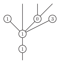
Figure 3. A stably-weighted tree. The tree has three inputs and total weight $6$. The corresponding operation is $(x_{1},x_{2},x_{3})\mapsto\mu^{1}_{1}(\mu^{1}_{4}(\mu^{1}_{0},x_{1},\mu^{0}_{2}(x_{2},x_{3}),\mu^{3}_{0}))$.

If $S$ and $T$ are stably-weighted trees, where $S$ has $n$ inputs, let $S\circ T=\sum_{i=1}^{n}S\circ_{i}T$. If $S_{1},S_{2},T_{1}$ and $T_{2}$ are stably-weighted trees so that $S_{1}$ and $S_{2}$ have the same number of inputs, let

$$(S_{1},S_{2})\circ(T_{1},T_{2})=\sum_{i=1}^{n}(S_{1}\circ_{i}T_{1},S_{2}\circ_{i}T_{2}).$$

We will sometimes also consider pairs of trees $(S_{1},S_{2})$ and $(T_{1},T_{2})$ where $S_{1}$ has $n$ inputs and $S_{2}$ has $n-1$, and define

$$(S_{1},S_{2})\circ^{\prime}(T_{1},T_{2})=\sum_{i=1}^{n-1}(S_{1}\circ_{i+1}T_{1},S_{2}\circ_{i}T_{2}).$$

1.3.3. Algebra diagonals and weighted type DD bimodules

Fix a weighted algebra $\mathcal{A}=(A,\{\mu_{n}^{w}\})$ over ${\mathbb{F}_{2}}[\mathcal{Y}_{1},\mathcal{Y}_{2}]$. In the case of bordered Floer homology, $\mathcal{Y}_{1}$ will act by $1$ and $\mathcal{Y}_{2}$ will act by $U$.

Given a stably-weighted tree $T$ with $n$ inputs there is an induced map $\mu(T)\nobreak\mskip 2.0mu\mathpunct{}\nonscript\mkern-3.0mu{:}\penalty 300\mskip 6.0mu plus 1.0muA^{\otimes n}\to A$ gotten by replacing each internal vertex $v$ of $T$ with valence $n+1$ and weight $w(v)$ by the operation $\mu_{n}^{w(v)}$, feeding the elements of $A^{\otimes n}$ into the inputs (in order), and composing according to the edges of the tree. (An example is shown in Figure 3.) So, given two weighted algebras $\mathcal{A}$, $\mathcal{B}$ and a pair of stably-weighted trees $(S,T)$ with $n$ inputs each, there is a corresponding map $\mu_{\mathcal{A}}(S)\otimes_{{\mathbb{F}_{2}}}\mu_{\mathcal{B}}(T)\nobreak\mskip 2.0mu\mathpunct{}\nonscript\mkern-3.0mu{:}\penalty 300\mskip 6.0mu plus 1.0mu(A\otimes_{{\mathbb{F}_{2}}}B)^{\otimes n}\cong A^{\otimes n}\otimes_{{\mathbb{F}_{2}}}B^{\otimes n}\to A\otimes_{{\mathbb{F}_{2}}}B$.

Definition 1.17.

[LOT20, Definition LABEL:Abs:def:wDiagCells] A weighted algebra diagonal consists of an element

$$\boldsymbol{\gamma}^{n,w}\in\bigoplus_{w_{1},w_{2}\leq w}\mathcal{Y}_{1}^{w-w_{1}}\mathcal{Y}_{2}^{w-w_{2}}\widetilde{X}_{*}^{n,w_{1}}\otimes_{{\mathbb{F}_{2}}}\widetilde{X}_{*}^{n,w_{2}}\subset\bigoplus_{w_{1},w_{2}\leq w}\widetilde{X}_{*}^{n,w_{1}}\otimes_{{\mathbb{F}_{2}}}\widetilde{X}_{*}^{n,w_{2}}\otimes_{{\mathbb{F}_{2}}}{\mathbb{F}_{2}}[\mathcal{Y}_{1},\mathcal{Y}_{2}]$$

of dimension $n+2w-2$, for each $n,m\geq 0$ with $n+2w\geq 2$, satisfying the following properties:

• Compatibility:

  (1.18) $$\partial\boldsymbol{\gamma}^{n,x}=\sum_{\begin{subarray}{c}v+w=x\\ 1\leq i\leq n\\ i-1\leq j\leq n\end{subarray}}\boldsymbol{\gamma}^{j-i+1,v}\circ\boldsymbol{\gamma}^{n+i-j,w}.$$

• Non-degeneracy:

  • $\boldsymbol{\gamma}^{2,0}=\Psi_{2}^{0}\otimes\Psi_{2}^{0}$.

  • $\boldsymbol{\gamma}^{0,1}=\Psi_{0}^{1}\otimes\Psi_{0}^{1}+\mathcal{Y}_{1}\top\otimes\Psi_{0}^{1}+\mathcal{Y}_{2}\Psi_{0}^{1}\otimes\top.$

  • At most one of each pair of trees in the diagonal is a degenerate tree.

(The second non-degeneracy property corresponds to specializing [LOT20, Definition LABEL:Abs:def:wDiagCells] to the diagonals with maximal seed.)

Given a weighted algebra diagonal $\boldsymbol{\Gamma}$ and weighted algebras $\mathcal{A}$ and $\mathcal{B}$ over ground rings $\mathds{k}$ and $\mathrlap{\hskip 1.25pt\mathrm{l}}{\mathrm{l}}$ over ${\mathbb{F}_{2}}[\mathcal{Y}_{1},\mathcal{Y}_{2}]$ we can form the tensor product $\mathcal{A}\otimes_{\boldsymbol{\Gamma}}\mathcal{B}$ with underlying $(\mathds{k}\otimes_{{\mathbb{F}_{2}}}\mathrlap{\hskip 1.25pt\mathrm{l}}{\mathrm{l}})$-module $A\otimes_{{\mathbb{F}_{2}}[\mathcal{Y}_{1},\mathcal{Y}_{2}]}B$, differential $\mu_{1}^{0}$ the usual tensor differential on the tensor product, and operations $\mu_{n}^{w}$ given by

$$\mu_{n}^{w}=\sum_{n_{S,T}(S\otimes T)\in\boldsymbol{\gamma}^{n,w}}n_{S,T}\mu_{\mathcal{A}}(S)\otimes\mu_{\mathcal{B}}(T).$$

It follows from the definition that this is, indeed, a weighted $A_{\infty}$-algebra (cf. [LOT20, Section LABEL:Abs:sec:w-alg-tens]). We now define a weighted type DD bimodule over $\mathcal{A}$ and $\mathcal{B}$ to be a weighted type $D$ module over $\mathcal{A}\otimes_{\boldsymbol{\Gamma}}\mathcal{B}$. (As was the case for type $D$ modules, we require some additional boundedness hypothesis to ensure this sum converges; see Section 7.2.)

Note that a weighted type DD bimodule is determined by a $(\mathds{k},\mathrlap{\hskip 1.25pt\mathrm{l}}{\mathrm{l}})$-bimodule $P$ and a map of $(\mathds{k},\mathrlap{\hskip 1.25pt\mathrm{l}}{\mathrm{l}})$-bimodules $\delta^{1}\nobreak\mskip 2.0mu\mathpunct{}\nonscript\mkern-3.0mu{:}\penalty 300\mskip 6.0mu plus 1.0muP\to(\mathcal{A}\otimes_{{\mathbb{F}_{2}}}\mathcal{B})\otimes P$; the structure equation that $\delta^{1}$ must satisfy depends on the diagonal $\boldsymbol{\Gamma}$.

In order to make use of this construction, we need to know that:

Theorem 1.19.

[LOT20, Theorem LABEL:Abs:thm:wDiag-exists] A weighted algebra diagonal exists.

1.3.4. The dualizing bimodule, and a graded miracle

Let $\mathcal{A}_{-}^{U=1}$ be the result of setting $U=1$ in $\mathcal{A}_{-}$. Fix a weighted algebra diagonal. View $\mathcal{A}_{-}$ as an algebra over ${\mathbb{F}_{2}}[\mathcal{Y}_{2}]$ by letting $\mathcal{Y}_{2}$ act by $U$, and $\mathcal{A}_{-}^{U=1}$ as an algebra over ${\mathbb{F}_{2}}[\mathcal{Y}_{1}]$ by letting $\mathcal{Y}_{1}$ act by $1$.

The dualizing bimodule $\mathit{CFDD}^{-}(\mathbb{I})$ is the type DD bimodule over $\mathcal{A}_{-}^{U=1}$ and $\mathcal{A}_{-}$ generated by two elements, $\iota_{0}\otimes\iota_{0}$ and $\iota_{1}\otimes\iota_{1}$, with differential $\delta^{1}$ given by

(1.20) $$\begin{split}\delta^{1}(\iota_{0}\otimes\iota_{0})&=(\rho_{1}\otimes\rho_{3}+\rho_{3}\otimes\rho_{1}+\rho_{123}\otimes\rho_{123}+\rho_{341}\otimes\rho_{341})\otimes(\iota_{1}\otimes\iota_{1})\\ \delta^{1}(\iota_{1}\otimes\iota_{1})&=(\rho_{2}\otimes\rho_{2}+\rho_{4}\otimes\rho_{4}+\rho_{234}\otimes\rho_{412}+\rho_{412}\otimes\rho_{234})\otimes(\iota_{0}\otimes\iota_{0})\end{split}$$

Even though we do not give a holomorphic curve interpretation of $\mathit{CFDD}^{-}(\mathbb{I})$ in this paper, the Heegaard diagram it corresponds to is helpful for understanding the terms that appear: see Figure 4.

By taking advantage of the gradings on $\mathcal{A}_{-}$, it is not hard to show that $\mathit{CFDD}^{-}(\mathbb{I})$ is, in fact, a type DD bimodule (again of charge 1 in the terminology of [LOT20]); see Section 7.1. In particular, although the bimodule structure relation depends on a weighted algebra diagonal, it turns out that the relation holds for any choice of weighted algebra diagonal.

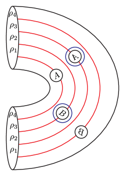
Figure 4. The type bimodule $\mathit{CFDD}^{-}(\mathbb{I})$. Although we do not associate bimodules to bordered Heegaard diagrams with two boundary components in this paper, we expect that the bimodule $\mathit{CFDD}^{-}(\mathbb{I})$ corresponds to this bordered Heegaard diagram, as $\widehat{\mathit{CFDD}}(\mathbb{I})$ does. The positive domains with index $1$ correspond to the terms in Formula (1.20). (Compare [LOT15, Proposition 10.1] or [LOT14, Theorem 1].)

1.4. First pairing theorem

1.4.1. More abstract algebra

Just as a weighted algebra diagonal allows us to take the external tensor product of weighted $A_{\infty}$-algebras, there is a notion of weighted module diagonals, which allows us to take the external tensor product of weighted modules. To state it, we need a variant of weighted trees. Given a stably-weighted tree $T$, the leftmost strand of $T$ is the minimal path from the leftmost input of $T$ to the root of $T$. A weighted module tree is a stably-weighted tree in which the leftmost leaf is an input; equivalently, a weighted module tree has no leaves to the left of its leftmost strand. The weighted module trees span a quotient complex $X\!M_{*}^{1+n,w}$ of the weighted trees complex $X_{*}^{1+n,w}$.

Definition 1.21.

[LOT20, Definition LABEL:Abs:def:w-mod-diag] Given a weighted algebra diagonal $\boldsymbol{\Gamma}$, a weighted module diagonal compatible with $\boldsymbol{\Gamma}$ is a formal linear combination of pairs of trees

$$\mathbf{m}^{n,w}\in\bigoplus_{w_{1},w_{2}\leq w}\mathcal{Y}_{1}^{w-w_{1}}\mathcal{Y}_{2}^{w-w_{2}}\widetilde{X\!M}_{*}^{n,w_{1}}\otimes_{{\mathbb{F}_{2}}}\widetilde{X\!M}_{*}^{n,w_{2}}\otimes_{{\mathbb{F}_{2}}}{\mathbb{F}_{2}}[\mathcal{Y}_{1},\mathcal{Y}_{2}]\\ \subset\bigoplus_{w_{1},w_{2}\leq w}\widetilde{X\!M}_{*}^{n,w_{1}}\otimes_{{\mathbb{F}_{2}}}\widetilde{X\!M}_{*}^{n,w_{2}}\otimes_{{\mathbb{F}_{2}}}{\mathbb{F}_{2}}[\mathcal{Y}_{1},\mathcal{Y}_{2}]$$

of dimension $n+2w-2$, satisfying the following conditions:

• Compatibility:

  (1.22) $$\partial\mathbf{m}^{n,x}=\sum_{v+w=x}\left(\sum_{j=1}^{n}\mathbf{m}^{n-j+1,v}\circ_{1}\mathbf{m}^{j,w}+\sum_{2\leq i\leq j\leq n}\mathbf{m}^{n+1+i-j,v}\circ_{i}\boldsymbol{\gamma}^{j-i,w}\right).$$

• Non-degeneracy: $\mathbf{m}^{2,0}=\Psi_{2}^{0}\otimes\Psi_{2}^{0}$.

Theorem 1.23.

[LOT20, Theorem LABEL:Abs:thm:wModDiag-exists] Given any weighted algebra diagonal $\boldsymbol{\Gamma}$ there is a weighted module diagonal compatible with $\boldsymbol{\Gamma}$.

Given a weighted module diagonal $\mathbf{m}$ and weighted (right) modules $\mathfrak{M}$, $\mathfrak{N}$ over weighted algebras $\mathcal{A}$, $\mathcal{B}$ (over $\mathds{k}$ and $\mathrlap{\hskip 1.25pt\mathrm{l}}{\mathrm{l}}$) the tensor product $\mathfrak{M}\otimes_{\mathbf{M}}\mathfrak{N}$ is the weighted (right) module over $\mathcal{A}\otimes_{\mathbf{M}}\mathcal{B}$ defined as follows. The underlying $(\mathds{k}\otimes_{{\mathbb{F}_{2}}}\mathrlap{\hskip 1.25pt\mathrm{l}}{\mathrm{l}})$-module is $M\otimes_{{\mathbb{F}_{2}}[\mathcal{Y}_{1},\mathcal{Y}_{2}]}N$. To define the operations on $\mathfrak{M}\otimes_{\mathbf{M}}\mathfrak{N}$, note that given a weighted $A_{\infty}$-module $(M,\{m_{1+n}^{w}\})$ over a weighted $A_{\infty}$-algebra $(A,\{\mu_{n}^{w}\})$ and a weighted module tree $T$ with $n+1$ inputs there is an induced map

$$m^{M}(T)\nobreak\mskip 2.0mu\mathpunct{}\nonscript\mkern-3.0mu{:}\penalty 300\mskip 6.0mu plus 1.0muM\otimes A^{\otimes n}\to M$$

defined by replacing each $(1+k)$-input, weight $w$ vertex on the leftmost strand of $T$ with the operation $m_{1+k}^{w}$ on $M$, every other $k$-input, weight $w$ vertex with the operation $\mu_{k}^{w}$ on $A$, and composing according to the tree. Then the operation $m_{1+n}^{w}$ on $M\otimes_{\mathbf{m}}N$ is defined by

$$m_{1+n}^{w}=\sum_{n_{S,T}(S\otimes T)\in\mathbf{m}^{1+n,w}}n_{S,T}\cdot m^{M}(S)\otimes m^{N}(T).$$

(The operation $m_{1}^{0}$ is the usual differential on the tensor product.)

Next, given a weighted module $M$ and weighted type $D$ structure $P$ over a weighted algebra $\mathcal{A}$, there is an associated chain complex $M\boxtimes_{\mathcal{A}}P$ with underlying module $M\otimes_{{\mathbb{F}_{2}}[\mathcal{Y}_{1},\mathcal{Y}_{2}]}P$ and differential

(1.24) $$\partial=\sum_{n,w\geq 0}(m_{1+n}^{w}\otimes\mathbb{I}_{P})\circ(\mathbb{I}_{M}\otimes\delta^{n}).$$

(Again, convergence requires some boundedness for $M$ and/or $P$; see Section 7.2.)

Proposition 1.25.

[LOT20, Lemmas LABEL:Abs:lem:w-DT-sq-0 and LABEL:Abs:lem:w-DT-bifunc] The endomorphism $\partial$ on $M\boxtimes P$ is, indeed, a differential. Moreover, changing $M$ or $P$ by a homotopy equivalence changes $M\boxtimes P$ by a homotopy equivalence.

Let $\mathcal{A}_{-}^{U=1}$ and $\mathit{CFA}^{-}_{U=1}(Y)$ be the result of setting $U=1$ on $\mathcal{A}_{-}$ and $\mathit{CFA}^{-}(Y)$, respectively. We are now able to state the first version of the pairing theorem, to be proved in a future paper:

Theorem 1.26.

[LOT] Given 3-manifolds $Y_{1}$ and $Y_{2}$ with $\partial Y_{1}=T^{2}=-\partial Y_{2}$, for any choice of weighted algebra and module diagonals there is a homotopy equivalence

$$\mathbf{CF}^{-}(Y_{1}\cup_{T^{2}}Y_{2})\simeq\bigl{(}\mathit{CFA}^{-}_{U=1}(Y_{1})\otimes_{\mathbf{M}}\mathbf{CFA}^{-}(Y_{2})\bigr{)}\boxtimes_{\mathcal{A}_{-}^{U=1}\otimes_{\boldsymbol{\Gamma}}\mathbfcal{A}_{-}}\mathit{CFDD}^{-}(\mathbb{I}).$$

(Here, $\mathbf{CFA}^{-}$ and $\mathbfcal{A}_{-}$ are completions of $\mathit{CFA}^{-}$ and $\mathcal{A}_{-}$; see Section 7.2.)

Remark 1.27.

Recall that for a general pointed matched circle, $\widehat{\mathit{CFDD}}(\mathbb{I})$ is a type DD bimodule over $\mathcal{A}(\mathcal{Z})$ and $\mathcal{A}(-\mathcal{Z})=\mathcal{A}(\mathcal{Z})^{\mathrm{op}}$ [LOT15, Section 8.1]. For the genus $1$ pointed matched circle, there is an isomorphism $\mathcal{A}(\mathcal{Z})\cong\mathcal{A}(-\mathcal{Z})$ exchanging $\rho_{1}$ and $\rho_{3}$ and fixing $\rho_{2}$ (and $\rho_{4}$). To obtain the type DD identity module described here, we have composed the action by $\mathcal{A}(-\mathcal{Z})$ with this isomorphism. (We did the same thing in [LOT15, Section 10.1]; in the notation of [LOT14, Section 3.1], $\rho_{3}$ is identified with $a_{o}(\rho_{1})$.)

1.5. Primitives and the type D module

In this subsection we sketch the definition of $\mathit{CFD}^{-}(\mathcal{H})$ and state a version of the pairing theorem closer to the pairing theorem for the hat case.

1.5.1. Module diagonal primitives and the definition of CFD

We will define $\mathit{CFD}^{-}(\mathcal{H})=\mathit{CFA}^{-}_{U=1}(\mathcal{H})\boxtimes\mathit{CFDD}^{-}(\mathbb{I})$, but making sense of this one-sided box product requires some additional abstract algebra and, before that, some additional forestry.

Definition 1.28.

[LOT20, Section LABEL:Abs:sec:w-prim] We describe here two ways to join a sequence of weighted trees together; the first is appropriate for trees in $X_{*}^{*,*}$ and the second for trees in $X\!M_{*}^{*,*}$. Specifically, given weighted trees $S_{1},\dots,S_{n}$ in $X_{*}^{*,*}$ their weight $w$ root joining $\operatorname{\operatorname{RoJ}}^{w}(S_{1},\dots,S_{n})$ is the result of adding a new root vertex with weight $w$ and feeding the outputs of $S_{1},\dots,S_{n}$ into the new vertex. The root joining is the sum over $w$ of $\mathcal{Y}_{1}^{w}$ times the weight $w$ root joining. In the special case $n=0$ (i.e., we are joining no trees) the root joining is the sum over $w>0$ of $\mathcal{Y}_{1}^{w}$ times the $0$-input, weight $w$ corolla.

Given weighted trees $T_{1},\dots,T_{n}$ in $X\!M_{*}^{*,*}$ their left joining $\operatorname{LeJ}(T_{1},\dots,T_{n})$ is obtained by feeding the output of each $T_{i}$ into the leftmost input of $T_{i+1}$. (One does not introduce a new $2$-valent vertex in this process.) In the special case that $n=0$ (i.e., we are joining no trees) we declare the left joining to be the generalized tree $\mathord{\downarrow}$.

So, the number of internal vertices of $\operatorname{\operatorname{RoJ}}^{w}(S_{1},\dots,S_{n})$ is one more than the sum of the numbers of internal vertices of $S_{1},\dots,S_{n}$, while the number of internal vertices of $\operatorname{LeJ}(T_{1},\dots,T_{n})$ is equal to the sum of the number of internal vertices of $T_{1},\dots,T_{n}$.

Combining these operations, given a sequence of pairs of trees $(T_{1},S_{1}),\dots,(T_{n},S_{n})$ in $X\!M_{*}^{*,*}\otimes_{{\mathbb{F}_{2}}}X_{*}^{*,*}$ so that for each $i$, $T_{i}$ has one more input than $S_{i}$, the left-root joining is

$$\operatorname{LR}((T_{1},S_{1}),\dots,(T_{n},S_{n}))=\operatorname{LeJ}(T_{1},\dots,T_{n})\otimes\operatorname{\operatorname{RoJ}}^{*}(S_{1},\dots,S_{n}).$$

The left-root joining is an element of (a completion of) $X\!M_{*}^{*,*}\otimes_{{\mathbb{F}_{2}}}X_{*}^{*,*}$.

There is a related operation which gives an element of $X\!M_{*}^{*,*}\otimes_{{\mathbb{F}_{2}}}X\!M_{*}^{*,*}$, defined by

$$\operatorname{LR}^{\prime}((T_{1},S_{1}),\dots,(T_{n},S_{n}))=\operatorname{LeJ}(T_{1},\dots,T_{n})\otimes\operatorname{\operatorname{RoJ}}^{*}(\mathord{\downarrow},S_{1},\dots,S_{n}).$$

Definition 1.29.

[LOT20, Definition LABEL:Abs:def:wM-prim] Given a weighted algebra diagonal $\boldsymbol{\Gamma}$, a weighted module diagonal primitive compatible with $\boldsymbol{\Gamma}$ consist of a linear combination of trees for $n\geq 1$ and $w\geq 0$, $(n,w)\neq(1,0)$, of the form

(1.30) $$\mathbf{p}^{n,w}=\sum_{(S,T)}(S,T)\in\bigoplus_{w_{1},w_{2}\leq w}\mathcal{Y}_{1}^{w-w_{1}}\mathcal{Y}_{2}^{w-w_{2}}\bigl{(}X\!M_{*}^{n,w_{1}}\otimes_{{\mathbb{F}_{2}}}\widetilde{X}_{*}^{n-1,w_{2}}\bigr{)},$$

of dimension $n+2w-2$, satisfying the following conditions:

• Compatibility:

  (1.31) $$\partial\mathbf{p}^{*,*}=\operatorname{LR}((\mathbf{p}^{*,*})^{\otimes\bullet})+\mathbf{p}^{*,*}\circ^{\prime}\boldsymbol{\gamma}^{*,*}.$$

  Here, $\mathbf{p}^{*,*}=\sum_{n,w}\mathbf{p}^{n,w}$ and $(\mathbf{p}^{*,*})^{\otimes\bullet}=\sum_{n\geq 0}(\mathbf{p}^{*,*})^{\otimes n}$.

• Non-degeneracy: $\mathbf{p}^{2,0}=\Psi_{2}^{0}\otimes\mathord{\downarrow}$.

Proposition 1.32.

[LOT20, Proposition LABEL:Abs:prop:wprim-exist] Given any weighted algebra diagonal, there is a compatible weighted module diagonal primitive.

From now on, fix a weighted algebra diagonal $\boldsymbol{\Gamma}$. For example, the proof of existence of weighted diagonals [LOT20, Lemma 5.3 and Theorem 6.11] induces a specific choice of weighted algebra diagonal, and we may fix that one throughout.

Definition 1.33.

[LOT20, Definition LABEL:Abs:def:wM-prim] Given a weighted module diagonal primitive, there is an associated weighted module diagonal defined by

$$\operatorname{LR}^{\prime}((\mathbf{p}^{*,*})^{\otimes\bullet}).$$

It is not hard to show that, for any weighted module diagonal primitive, this defines a weighted module diagonal [LOT20, Lemma LABEL:Abs:lem:wprim-gives-diag].

In the following definition, for notational reasons, we view a left-left type DD bimodules $P$ over $\mathcal{A}$ and $\mathcal{B}$ as a left-right type DD bimodule over $\mathcal{A}$ and $\mathcal{B}^{\mathrm{op}}$.

Definition 1.34.

[LOT20, Definition LABEL:Abs:def:w-one-sided-DT] Given a weighted module diagonal primitive $\mathbf{p}$ compatible with the weighted algebra diagonal $\boldsymbol{\Gamma}$, weighted algebras $\mathcal{A}$ and $\mathcal{B}$, a weighted module $\mathfrak{M}$ over $\mathcal{A}$, and a weighted type DD bimodule $P$ over $\mathcal{A}$ and $\mathcal{B}$ (compatible with $\boldsymbol{\Gamma}$), we define the one-sided box tensor product of $\mathfrak{M}$ and $P$,

$$\mathfrak{M}\boxtimes_{\mathcal{A}}P,$$

to be the weighted type $D$ structure $(M\otimes_{\mathds{k}}P,\delta^{1})$ where $\delta^{1}$ is given by

$$\delta^{1}(x\otimes y)=m_{1}^{0}(x)\otimes y\otimes 1+\sum_{n,w\geq 0}\sum_{(S,T)\in\mathbf{p}^{n,w}}(m^{M}(S)\otimes\mathbb{I}_{P}\otimes\mu^{\mathcal{B}^{\mathrm{op}}}(T^{\mathrm{op}}))\circ(\mathbb{I}_{M}\otimes\delta_{P}).$$

The fact that this defines a weighted type $D$ structure is [LOT20, Proposition LABEL:Abs:prop:one-sided-DT-works]. (Again, we have specialized to the charge-1 case. Also, we again need some boundedness to ensure the sums converge; see Section 7.2.)

Recall that we have fixed a weighted algebra diagonal $\boldsymbol{\Gamma}$. Given a weighted module diagonal primitive $\mathbf{p}$ compatible with $\boldsymbol{\Gamma}$, define

$$\mathit{CFD}^{-}(\mathcal{H})=\mathit{CFA}^{-}_{U=1}(\mathcal{H})\boxtimes_{\mathcal{A}_{-}^{U=1}}\mathit{CFDD}^{-}(\mathbb{I}).$$

Theorem 1.35.

The object $\mathit{CFD}^{-}(\mathcal{H})$ is a weighted type $D$ structure. Further, up to homotopy equivalence, $\mathit{CFD}^{-}(\mathcal{H})$ depends on $\mathcal{H}$ only through the bordered 3-manifold it specifies, and is independent of the choice of weighted module diagonal primitive $\mathbf{p}$.

This invariance theorem follows from the fact that $\mathit{CFA}^{-}$ is a weighted $A_{\infty}$-module (Theorem 6.25), invariance of $\mathit{CFA}^{-}$ (Theorem 1.14), and abstract algebra (specifically, [LOT20, Lemma LABEL:Abs:lem:w-one-side-DT-id-chain-map and Corollary LABEL:Abs:cor:w-DT-preserve-hequiv]).

1.5.2. Second pairing theorem

Theorem 1.36.

[LOT] Given 3-manifolds $Y_{1}$ and $Y_{2}$ with $-\partial Y_{1}=T^{2}=\partial Y_{2}$, there is a homotopy equivalence

$$\mathbf{CF}^{-}(Y_{2}\cup_{T^{2}}Y_{1})\simeq\mathbf{CFA}^{-}(Y_{2})\boxtimes\mathit{CFD}^{-}(Y_{1}).$$

This follows from the definitions, Theorem 1.26 (whose proof will be given in [LOT]), and abstract algebra (specifically, [LOT20, Proposition LABEL:Abs:prop:one-sided-DT-works]).

Related work

There are several other approaches to giving a bordered extension of ${\mathit{HF}}^{-}$. Zemke has given a construction of an algebra associated to the torus and type $D$ and $A$ modules associated to 3-manifolds with torus boundary, satisfying a pairing theorem [Zema], with both computational and conceptual applications [Zema, Zemb]. His construction begins from the link surgery theorem [MO10], and both repackages and extends that result. The relationship of his construction to the construction given here, or indeed to the $\widehat{\mathit{HF}}$ case of bordered Floer homology, is currently unknown.

Hanselman-Rasmussen-Watson have given a reformulation of the $\widehat{\mathit{HF}}$ case of bordered Floer homology with torus boundary in terms of immersed curves in the torus [HRW16]. Their construction starts from $\mathcal{A}$, $\widehat{\mathit{CFD}}$, and $\widehat{\mathit{CFA}}$, and the invariance and pairing results for classical bordered Floer homology are ingredients in their reformulation. Recently, Hanselman has used the rational surgery formula [OSz11] to refine this immersed curve invariant to compute ${\mathit{HF}}^{-}$, by equipping it with an appropriate local system over ${\mathbb{F}_{2}}[U]$ [Han23].

Acknowledgments

We thank Rumen Zarev for helpful conversations. The proofs of stabilization invariance in Sections 4.3 and 5.5 are adapted from a book in progress by András Stipsicz, Zoltán Szabó, and the second author, and we thank them for helpful conversations. We also thank Wenzhao Chen, Jonathan Hanselman, and Shikhin Sethi for comments on an early draft of this paper.

2. Background

2.1. Topological preliminaries

The topological context for the ${\mathbf{HF}}^{-}$ version of bordered Floer homology—the notions of Heegaard diagrams, $\operatorname{spin}^{c}$-structures, and so on—is the same as the setting for the original, $\widehat{\mathit{HF}}$ version [LOT18]. For the reader’s convenience, we recall briefly much of that terminology. The differences from our previous monograph are summarized at the end of the section.

The unique genus $1$ pointed matched circle, shown in Figure 5, consists of an oriented circle $Z$, $4$ points $\mathbf{a}\subset Z$, and one additional basepoint $z\in Z\setminus\mathbf{a}$. Order the points in $\mathbf{a}$ as $a_{1},a_{2},a_{3},a_{4}$ using the orientation of $Z$ and so that $z$ lies between $a_{4}$ and $a_{1}$. We view the points as matched in pairs, $a_{1}\leftrightarrow a_{3}$ and $a_{2}\leftrightarrow a_{4}$. When referring to $a_{i}$ we view the index $i$ as an element of $\mathbb{Z}/4\mathbb{Z}$. A Reeb chord (or simply chord) in $Z$ is a homotopy class of orientation-preserving maps $\rho\nobreak\mskip 2.0mu\mathpunct{}\nonscript\mkern-3.0mu{:}\penalty 300\mskip 6.0mu plus 1.0mu([0,1],\{0,1\})\to(Z,\mathbf{a})$. There are four short Reeb chords $\rho_{1},\dots,\rho_{4}$, where $\rho_{i}$ has endpoints $a_{i}$ and $a_{i+1}$ and is otherwise disjoint from $\mathbf{a}$; we will view the indices $i$ of the $\rho_{i}$ as elements of $\mathbb{Z}/4\mathbb{Z}$ as well.

Figure 5. The genus $1$ pointed matched circle.

A Reeb chord $\rho$ has an initial endpoint $\rho^{-}=\rho(0)$ and a terminal endpoint $\rho^{+}=\rho(1)$. Reeb chords $\rho$ and $\sigma$ are consecutive if $\rho^{+}=\sigma^{-}$. Consecutive Reeb chords can be concatenated; we write the concatenation of $\rho$ and $\sigma$ as $\rho\sigma$. (In [LOT18] we wrote the concatenation of $\rho$ and $\sigma$ as $\rho\uplus\sigma$ because we also considered sets of Reeb chords, but in the present setting $\rho\sigma$ will not cause confusion.) Any Reeb chord can be obtained by successively concatenating the four short Reeb chords, and we often write $\rho_{i\dots j}$ to denote the concatenation $\rho_{i}\rho_{i+1}\cdots\rho_{j}$. A Reeb chord $\rho$ has a support $\boldsymbol{[}\rho\boldsymbol{]}\in H_{1}(Z,\mathbf{a})$. We will also often consider sequences $\vec{\rho}=(\rho^{1},\dots,\rho^{n})$ of Reeb chords; the support of such a sequence is $\boldsymbol{[}\vec{\rho}\boldsymbol{]}=\boldsymbol{[}\rho^{1}\boldsymbol{]}+\cdots+\boldsymbol{[}\rho^{n}\boldsymbol{]}$.

A bordered Heegaard diagram consists of a compact, oriented surface-with-boundary $\Sigma$, whose genus is denoted $g$; two arcs $\alpha_{1}^{a},\alpha_{2}^{a}\subset\Sigma$ with boundary on $\partial\Sigma$; $g-1$ circles $\alpha_{1}^{c},\dots,\alpha_{g-1}^{c}$ and $g$ circles $\beta_{1},\dots,\beta_{g}$ in the interior of $\Sigma$; and a basepoint $z\in\partial\Sigma$ that is not an endpoint of either $\alpha_{i}^{a}$. All of the $\alpha$-curves are required to be disjoint from each other, as are all of the $\beta$-circles. If we let ${\boldsymbol{\alpha}}$ (respectively ${\boldsymbol{\beta}}$) be the union of the $\alpha$-curves (respectively $\beta$-circles), then $\Sigma\setminus{\boldsymbol{\alpha}}$ and $\Sigma\setminus{\boldsymbol{\beta}}$ are required to be connected. We will also typically assume that ${\boldsymbol{\alpha}}\pitchfork{\boldsymbol{\beta}}$. (Unlike [LOT18], we consider here only bordered Heegaard diagrams for 3-manifolds with genus $1$ boundary.)

The (oriented) boundary of a bordered Heegaard diagram $\mathcal{H}=(\Sigma,{\boldsymbol{\alpha}},{\boldsymbol{\beta}},z)$ is the genus $1$ pointed matched circle. In particular, each Reeb chord in the genus $1$ pointed matched circle corresponds to an arc in $(\partial\Sigma,{\boldsymbol{\alpha}}\cap\partial\Sigma)$. Given a chord $\rho$, we let $[\rho^{-}]$ (respectively $[\rho^{+}]$) be the $\alpha$-arc containing the initial (respectively terminal) endpoint of $\rho$.

From a bordered Heegaard diagram one can construct a 3-manifold whose boundary is identified with a standard torus—i.e., a bordered 3-manifold (with torus boundary); we refer to our monograph [LOT18, Construction 4.6] for the construction. Up to diffeomorphism (rel boundary), every bordered 3-manifold with torus boundary arises this way [LOT18, Lemma 4.9]. Two bordered Heegaard diagrams represent diffeomorphic bordered 3-manifolds if and only if they become diffeomorphic as diagrams after a sequence of isotopies, handleslides among the $\beta$-circles or of $\alpha$-arcs or circles over $\alpha$-circles, and stabilizations [LOT18, Proposition 4.10]. (These moves are collectively called Heegaard moves.)

Given a bordered Heegaard diagram $\mathcal{H}$, a generator (for the bordered Floer modules) is a $g$-tuple of points $\mathbf{x}=\{x_{i}\}_{i=1}^{g}\subset{\boldsymbol{\alpha}}\cap{\boldsymbol{\beta}}$ so that $\mathbf{x}$ has exactly one point on each $\alpha$-circle and each $\beta$-circle and, consequently, one point on one of the two $\alpha$-arcs. Let $\mathfrak{S}(\mathcal{H})$ denote the set of generators for $\mathcal{H}$.

Given generators $\mathbf{x}$ and $\mathbf{y}$, let $\pi_{2}(\mathbf{x},\mathbf{y})$ denote the set of homology classes, or domains, connecting $\mathbf{x}$ to $\mathbf{y}$. That is, an element of $\pi_{2}(\mathbf{x},\mathbf{y})$ is a linear combination $B$ of connected components of $\Sigma\setminus({\boldsymbol{\alpha}}\cup{\boldsymbol{\beta}})$ (regions) satisfying the following condition. Let $\partial^{\alpha}(B)$ (respectively $\partial^{\beta}(B)$, $\partial^{\partial}(B)$) denote the part of $\partial(B)$ lying in ${\boldsymbol{\alpha}}$ (respectively ${\boldsymbol{\beta}}$, $\partial\Sigma$). Then, $B\in\pi_{2}(\mathbf{x},\mathbf{y})$ if and only if $\partial(\partial^{\beta}(B))=\mathbf{x}-\mathbf{y}$. Equivalently, $B$ is an element of

$$H_{2}(\Sigma\times[0,1]\times[-1,1],\mathbf{x}\times[0,1]\times\{-1\}\cup\mathbf{y}\times[0,1]\times\{1\}\\ \cup{\boldsymbol{\beta}}\times\{0\}\times[-1,1]\cup({\boldsymbol{\alpha}}\cup\partial\Sigma)\times\{1\}\times[-1,1])$$

so that the projection of $\partial B$ to $H_{1}(\mathbf{x}\times[0,1]\times\{-1\},\mathbf{x}\times\{0,1\}\times\{-1\})=\mathbb{Z}^{g}$ is $(1,\dots,1)$, and similarly for $\mathbf{y}$. Note that unlike in our monograph [LOT18], we do not require that $B$ have multiplicity $0$ at the region adjacent to $z$.

A domain $B$ has a multiplicity $n_{z}(B)$ at the region adjacent to $z$. A periodic domain is an element of $\pi_{2}(\mathbf{x},\mathbf{x})$ (for some generator $\mathbf{x}$) with $n_{z}(B)=0$. A domain $B$ is provincial if $\partial^{\partial}(B)=0$. The set of periodic domains is in canonical bijection with $H_{2}(Y,\partial Y)$ (where $Y$ is the 3-manifold specified by the Heegaard diagram); and the set of provincial periodic domains is in canonical bijection with $H_{2}(Y)$. The boundary of a domain $B$, $\partial^{\partial}B$, is an element of $\mathbb{Z}^{4}$, via the multiplicities at $\rho_{1}$, $\rho_{2}$, $\rho_{3}$, and $\rho_{4}$, respectively. Let $n_{p}(B)$ be the average multiplicity of $B$ at the boundary (or the puncture $p$). That is, if $\partial^{\partial}B=(a,b,c,d)$ then $n_{p}(B)=(a+b+c+d)/4$. (In this notation, $n_{z}(B)=d$.)

There is a concatenation map $\pi_{2}(\mathbf{w},\mathbf{x})\times\pi_{2}(\mathbf{x},\mathbf{y})\to\pi_{2}(\mathbf{w},\mathbf{y})$ which we will either write as $(B_{1},B_{2})\mapsto B_{1}*B_{2}$ or $(B_{1},B_{2})\mapsto B_{1}+B_{2}$, depending on the context.

A bordered Heegaard diagram is called provincially admissible if every non-zero provincial periodic domain has both positive and negative coefficients, and admissible if every periodic domain has both positive and negative coefficients. Every bordered Heegaard diagram is isotopic to an admissible one, and any two admissible (respectively provincially admissible) Heegaard diagrams can be connected by a sequence of Heegaard moves through admissible (respectively provincially admissible) diagrams [LOT18, Proposition 4.25] (whose proof is cited to [OSz04, Section 5]).

Every generator $\mathbf{x}$ represents a $\operatorname{spin}^{c}$-structure $\mathfrak{s}(\mathbf{x})\in\operatorname{spin}^{c}(Y)$ [LOT18, Section 4.3]. Further, $\mathfrak{s}(\mathbf{x})=\mathfrak{s}(\mathbf{y})$ if and only if $\pi_{2}(\mathbf{x},\mathbf{y})\neq\emptyset$ [LOT18, Lemma 4.21]. (In [LOT18], we consider only domains with multiplicity $0$ at $z$, but since we can add copies of $[\Sigma]$ to the domain, $\pi_{2}(\mathbf{x},\mathbf{y})\neq\emptyset$ if and only if there is a $B\in\pi_{2}(\mathbf{x},\mathbf{y})$ with $n_{z}(B)=0$.) If $\mathfrak{s}(x)=\mathfrak{s}(y)$, the set $\pi_{2}(\mathbf{x},\mathbf{y})$ is an affine copy of $\mathbb{Z}\oplus H_{2}(Y,\partial Y)$.

When considering holomorphic curves, we will attach a cylindrical end to $\partial\Sigma$, giving a non-compact surface with a single end. We will abuse notation and denote that surface by $\Sigma$, as well; it will be clear from context which of the two versions of $\Sigma$ we are discussing. We can think of this non-compact $\Sigma$ as a closed surface $\overline{\Sigma}$ minus a point $p$, and will often refer to the puncture (point at infinity) of $\Sigma$ as $p$. The non-compact version of $\Sigma$ still has a circle at infinity, and we can talk about Reeb chords in that circle (which are the same as the Reeb chords for the compact version).

We recapitulate the conventions that differ in this paper from our monograph [LOT18]:

• In this paper, the only pointed matched circle we consider is the (unique) pointed matched circle representing the torus, and we consider only the middle strands grading. So, the algebra $\mathcal{A}$ here is sometimes denoted $\mathcal{A}(\mathcal{Z}_{1},0)$ or $\mathcal{A}(T^{2},0)$ in the literature.

• We have dropped the notation $\uplus$ from concatenation of Reeb chords.

• The notation $\pi_{2}(x,y)$ denotes all domains connecting $x$ and $y$, not just those with $n_{z}=0$.

• We are not distinguishing in the notation between the compact surface-with-boundary $\Sigma$ (denoted $\overline{\Sigma}$ in [LOT18]) and the result of attaching a cylindrical end to it (denoted $\Sigma$ in [LOT18]). We are using $\overline{\Sigma}$ to denote the one-point compactification of the non-compact surface $\Sigma$. (This was denoted $\Sigma_{\overline{e}{}}$ in [LOT18].)

2.2. $G$-set gradings on weighted algebras, modules and type $D$ structures

Like the $\widehat{\mathit{HF}}$ case, the algebra $\mathcal{A}_{-}$ is graded by a non-commutative group with a distinguished central element, and the modules $\mathit{CFA}^{-}$ and $\mathit{CFD}^{-}$ are graded by sets with right- and left-actions by this group, respectively. Also like the $\widehat{\mathit{HF}}$ case, there are several natural choices for the non-commutative group. In this section we describe what a group-valued grading on a weighted module or type $D$ structure means abstractly; the gradings on $\mathit{CFA}^{-}$ and $\mathit{CFD}^{-}$ themselves are constructed in Section 8. In Section 2.3 we recall one of the options for a grading group. (This material is used in Sections 7.1 and 8.)

Fix a group $G$ and central elements $\lambda_{d},\lambda_{w}\in G$. We call $\lambda_{w}$ the weight grading; when $\lambda_{w}$ is the identity element of $G$ then we will often write $\lambda_{d}$ simply as $\lambda$. Recall that a $(G,\lambda_{d},\lambda_{w})$-graded weighted algebra is a weighted algebra $\mathcal{A}=(A,\{\mu_{n}^{w}\})$ together with subspaces $A_{g}\subset A$, $g\in G$, of homogeneous elements of grading $g$, so that $A_{g}\cap A_{h}=\{0\}$ if $g\neq h$ and

(2.1) $$\mu_{n}^{k}\nobreak\mskip 2.0mu\mathpunct{}\nonscript\mkern-3.0mu{:}\penalty 300\mskip 6.0mu plus 1.0muA_{g_{1}}\otimes\cdots\otimes A_{g_{n}}\to A_{\lambda_{d}^{n-2}\lambda_{w}^{k}g_{1}\cdots g_{n}}$$

[LOT21, Section LABEL:TA:sec:W-gradings]. That is, if we write $\operatorname{gr}(a)=g$ whenever $a\in A_{g}$ then

$$\operatorname{gr}(\mu_{n}^{k}(a_{1},\dots,a_{n}))=\lambda_{d}^{n-2}\lambda_{w}^{k}\operatorname{gr}(a_{1})\cdots\operatorname{gr}(a_{n}).$$

We will assume that either $A=\bigoplus_{g\in G}A_{g}$ (i.e., is generated by the homogeneous elements), or is the completion of $\bigoplus_{g\in G}A_{g}$ with respect to some filtration. (The former will be the case for $\mathcal{A}_{-}$ and the latter for its completion $\mathbfcal{A}_{-}$ used in Section 7.)

Given a set $S$ with a right action of $G$, a grading of a weighted right module $\mathfrak{M}=(M,\{m_{1+n}^{k}\})$ by $S$ is a collection of subspaces $M_{s}\subset M$, $s\in S$, so that $M_{s}\cap M_{t}=\{0\}$ if $s\neq t$ and

$$m_{1+n}^{k}\nobreak\mskip 2.0mu\mathpunct{}\nonscript\mkern-3.0mu{:}\penalty 300\mskip 6.0mu plus 1.0muM_{s}\otimes A_{g_{1}}\otimes\cdots\otimes A_{g_{n}}\to M_{s\cdot\lambda_{d}^{n-1}\lambda_{w}^{k}g_{1}\cdots g_{n}}.$$

Writing $\operatorname{gr}(M_{s})=s$, this is equivalent to

$$\operatorname{gr}(m_{1+n}^{k}(\mathbf{x},a_{1},\dots,a_{n}))=\operatorname{gr}(\mathbf{x})\cdot\lambda_{d}^{n-1}\lambda_{w}^{k}\operatorname{gr}(a_{1})\cdots\operatorname{gr}(a_{n}).$$

Again, we assume that either $M=\bigoplus_{s\in S}M_{s}$ or that $M$ is the completion of this direct sum with respect to a filtration.

Given a set $S$ with a left action by $G$, a grading of a weighted type $D$ structure $(P,\delta^{1}\nobreak\mskip 2.0mu\mathpunct{}\nonscript\mkern-3.0mu{:}\penalty 300\mskip 6.0mu plus 1.0muP\to A\otimes P)$ by $G$ consists of subspaces $P_{s}$, $s\in S$, satisfying $P_{s}\cap P_{t}=\{0\}$ if $s\neq t$ and

$$\delta^{1}\nobreak\mskip 2.0mu\mathpunct{}\nonscript\mkern-3.0mu{:}\penalty 300\mskip 6.0mu plus 1.0muP_{s}\to\bigoplus_{g\cdot t=s}\lambda_{d}^{-1}A_{g}\otimes P_{t}.$$

That is, writing $\operatorname{gr}(P_{s})=s$,

$$\operatorname{gr}(\delta^{1}(x))=\lambda_{d}^{-1}\operatorname{gr}(x).$$

We again assume that either $P=\bigoplus_{s\in S}P_{s}$ or that $P$ is the completion of this direct sum with respect to a filtration.

Given weighted algebras $\mathcal{A}$ and $\mathcal{A}^{\prime}$ graded by $(G,\lambda_{d},\lambda_{w})$ and $(G^{\prime},\lambda_{d}^{\prime},\lambda_{w}^{\prime})$, and a weighted algebra diagonal, the tensor product $\mathcal{A}\otimes\mathcal{A}^{\prime}$ inherits a grading by the group $G\times_{\mathbb{Z}}G^{\prime}=G\times G^{\prime}/\langle\lambda_{d}^{-1}\lambda_{d}^{\prime}\rangle$ with central elements $\lambda_{d}=\lambda_{d}^{\prime}$ and $\lambda_{w}\lambda_{w}^{\prime}\lambda_{d}^{-2}$ (compare [LOT20, Section LABEL:Abs:sec:w-alg-tens]). Here, we assume that the variables $\mathcal{Y}_{1}$ and $\mathcal{Y}_{2}$ in the definition of a weighted diagonal—see Section 1.3.3—have gradings $\lambda_{d}^{-2}\lambda_{w}$ and $(\lambda_{d}^{\prime})^{-2}\lambda_{w}^{\prime}$, respectively. This gives rise to the notion of a graded, weighted type DD structure $P$ over $\mathcal{A}$ and $\mathcal{A}^{\prime}$, graded by a left $(G\times_{\mathbb{Z}}G^{\prime})$-set $T$.

Continuing in this vein, given a weighted DD structure $P$ as above and a weighted module $\mathfrak{M}$ graded by the $G$-set $S$, the one-sided box product $\mathfrak{M}\boxtimes P$ is graded by the $G^{\prime}$-set $S\times_{G}T$ [LOT20, Proposition LABEL:Abs:prop:one-sided-DT-works]. Given another weighted module $\mathfrak{M}^{\prime}$ graded by the $G^{\prime}$-set $S^{\prime}$, the triple box product $\mathfrak{M}\boxtimes P\boxtimes\mathfrak{M}^{\prime}$ is graded by the $\mathbb{Z}$-set $(S\times_{G}T\times_{G^{\prime}}(S^{\prime})^{\mathrm{op}},\lambda_{d}=\lambda_{d}^{\prime})$.

2.3. The big grading group

Because we will need it in Section 7.1, we recall the definition of the big grading group $G^{\prime}$ [LOT21, Section LABEL:TA:sec:big-group] (also recalled in the introduction). Other options for gradings are discussed in Section 8.

Consider the group ${\textstyle\frac{1}{2}}\mathbb{Z}\times\mathbb{Z}^{4}$ with multiplication

$$(m;a,b,c,d)\cdot(m^{\prime};a^{\prime},b^{\prime},c^{\prime},d^{\prime})\\ =\left(m+m^{\prime}+{\textstyle\frac{1}{2}}\left|\begin{smallmatrix}a&b\\ a^{\prime}&b^{\prime}\end{smallmatrix}\right|+{\textstyle\frac{1}{2}}\left|\begin{smallmatrix}b&c\\ b^{\prime}&c^{\prime}\end{smallmatrix}\right|+{\textstyle\frac{1}{2}}\left|\begin{smallmatrix}c&d\\ c^{\prime}&d^{\prime}\end{smallmatrix}\right|+{\textstyle\frac{1}{2}}\left|\begin{smallmatrix}d&a\\ d^{\prime}&a^{\prime}\end{smallmatrix}\right|,a+a^{\prime},b+b^{\prime},c+c^{\prime},d+d^{\prime}\right).$$

The elements

$$\operatorname{gr}^{\prime}(\rho_{1}) =(-1/2;1,0,0,0) \operatorname{gr}^{\prime}(\rho_{2}) =(-1/2;0,1,0,0)$$

$$\operatorname{gr}^{\prime}(\rho_{3}) =(-1/2;0,0,1,0) \operatorname{gr}^{\prime}(\rho_{4}) =(-1/2;0,0,0,1)$$

$$\lambda =(1;0,0,0,0)$$

generate an index-2 subgroup of this group, which we denote $G^{\prime}$. A grading $\operatorname{gr}^{\prime}$ on the algebra $\mathcal{A}_{-}$ by $G^{\prime}$ is determined by the gradings of the $\rho_{i}$ and $\operatorname{gr}^{\prime}(U)=(-1;1,1,1,1)$. We will call the first entry in the grading the Maslov component, and the remaining four the $\operatorname{spin}^{c}$ component. For a Reeb chord $\rho$, the $\operatorname{spin}^{c}$ component of $\operatorname{gr}^{\prime}(\rho)$ is just the support of $\rho$, while the Maslov component is $-|\rho|/4$ if $|\rho|$ is divisible by $4$, and $-1/2-\lfloor|\rho|/4\rfloor$ otherwise. (This is also $\iota(\rho)$ from Eq. (3.26).) For this grading, the central element is $\lambda_{d}=\lambda=(1;0,0,0,0)$ and the weight grading is $\lambda_{w}=(1;1,1,1,1)$. (Note that $\operatorname{gr}^{\prime}(U)=\operatorname{gr}^{\prime}(\rho_{1234})$ and $\lambda_{w}=\lambda^{2}\operatorname{gr}^{\prime}(U)$, so both lie in $G^{\prime}$.)

2.4. The associaplex

In the course of studying the algebraic background behind weighted $A_{\infty}$-algebras, we introduced a CW complex called the (weighted) associaplex [LOT20, Sec. 8].

Recall that the associahedron, relevant to $A_{\infty}$-algebras, is a polytope that is a compactification of the space of $n+1$ points on $\partial D^{2}$, one of which is distinguished (or equivalently of $n$ points on a line), modulo symmetries. The associaplex ${\mathbf{X}}^{n,w}$, relevant to weighted $A_{\infty}$-algebras, is instead a compactification of the space of $w$ distinct, unordered points in the interior of $D^{2}$ and $n+1$ points in $\partial D^{2}$, one of which is distinguished, again modulo symmetries (Möbius transformations). The most familiar compactification is the Deligne-Mumford compactification, which adds strata corresponding to decompositions into disks and spheres connected at nodes, each with enough special points to be stable. The Deligne-Mumford compactification recovers the associahedron when all the points are on the boundary, but records more information than we need about interior points, so ${\mathbf{X}}^{n,w}$ is obtained from the Deligne-Mumford compactification by collapsing all the spheres. So, interior marked points collide as in a symmetric product, recording just the multiplicities. On the boundary, more information is remembered, through disks bubbling off. We refer the reader to our previous paper [LOT20, Section 8] for further details, and a direct construction not using the Deligne-Mumford compactification.

3. Moduli spaces of holomorphic curves

The main goal of this section is to prove Theorem 1.12, the workhorse technical result guaranteeing that $\mathit{CFA}^{-}$ and $\mathit{CFD}^{-}$ are well-defined. We start with some examples, in Section 3.1, to illustrate the kinds of codimension-1 degenerations which occur; this section is not needed for the rest of the paper. The work starts in Section 3.2, where we define the various moduli spaces. Key to that is the formulation of the families of almost complex structures we will use, in Section 3.2.1. Next, we compute the expected dimensions of the moduli spaces, in Section 3.3. Section 3.4 formulates a condition, being sufficiently pinched, that is required to guarantee that boundary degenerations correspond to operations on the algebra. (Part of the proof that condition suffices is in Section 4.) In Section 3.5, we show that for appropriate families of almost complex structures, most of the moduli spaces are transversely cut out by the $\bar{\partial}$-equations. (Again, a few remaining cases are deferred to Section 4.) Section 3.6 collects the gluing results we will need, showing that near various kinds of broken holomorphic curves the moduli space behaves like a manifold-with-boundary. Finally, Section 3.7 combines these ingredients to prove Theorem 1.12.

Throughout this section we fix a bordered Heegaard diagram $\mathcal{H}=(\Sigma,\alpha_{1}^{a},\alpha_{2}^{a},{\boldsymbol{\alpha}}^{c},{\boldsymbol{\beta}},z)$ with genus $g$.

3.1. Some examples

Before diving into the section’s work, we describe examples of the different degenerations in Theorem 1.12. We will refer to these examples later in the section to elucidate some of the more complicated definitions. Definitions of the moduli spaces discussed here are given in Section 3.2, but a reader familiar with bordered Floer homology can likely read this section without having read those definitions first.

The first two kinds of degenerations in Theorem 1.12 are familiar from the $\widehat{\mathit{HF}}$ case. For example, consider the genus-1 bordered Heegaard diagram and domain shown in Figure 6. The moduli space shown is denoted $\mathcal{M}^{B}(x,y;\rho_{3},\rho_{4},\rho_{3},\rho_{2},\rho_{12};0)$, where $B$ is the domain. (The $0$ denotes that there are no orbits on this curve, only chords.) The moduli space is 1-dimensional, corresponding to the location of the boundary branch point (end of the cut). As the branch point approaches the chord $\rho_{34}$ (cut shrinks to zero) the chords $\rho_{3}$ and $\rho_{4}$ come together, degenerating a split curve, just as would happen for bordered $\widehat{\mathit{HF}}$; this is a collision end. The main component of the result is an element of $\mathcal{M}^{B}(x,y;\rho_{34},\rho_{3},\rho_{2},\rho_{12};0)$. (In general, the chords involved in the split curve degeneration can be arbitrarily long.) Another collision end (and split curve) occurs in Figure 8 when the branch point approaches $\rho_{34}$; we discuss the other ends of these examples after giving another example.

Consider the Heegaard diagram and domain shown in Figure 7. Here, the domain $B$ has multiplicity $1$ everywhere in the diagram; the curve is an element of $\mathcal{M}^{B}(x,x;\rho_{4},\rho_{3},\rho_{2},\rho_{1};0)$. As the branch point approaches the left edge of the rectangle, the curve breaks as a two-story building, with the bottom story in $\mathcal{M}^{B_{1}}(x,x;\rho_{4},\rho_{3};0)$ and the top story in $\mathcal{M}^{B_{2}}(x,x;\rho_{2},\rho_{1};0)$. Again, this kind of degeneration (but not this particular domain) occurs in the $\widehat{\mathit{HF}}$ case. Indeed, this is the kind of degeneration that corresponds most closely to broken flows in Morse theory.

The remaining ends are new. In Figure 7, as the branch point approaches the right boundary of the rectangle (cut shrinks to zero), the curve degenerates into a component with boundary entirely in the $\alpha$-curves (a boundary degeneration) and a bigon mapped to $x$ by a constant map (a trivial strip). Let $\mathbb{H}$ denote the half-plane $\mathbb{H}=(-\infty,1]\times\mathbb{R}=\{x+iy\mid x\leq 1\}$. By rescaling, the component with boundary entirely in the $\alpha$-curves inherits a map to $(\Sigma\times\mathbb{H},{\boldsymbol{\alpha}}\times\{1\}\times\mathbb{R})$, asymptotic at $\infty$ in $\mathbb{H}$ to the point $x$. This is an element in $\mathcal{N}(x;\rho_{4},\rho_{3},\rho_{2},\rho_{1};0)$, and is called a simple boundary degeneration.

In Figure 6, when the branch point approaches $\rho_{12}$ (i.e., the cut becomes as long as possible), the curve splits into a main component, in $\mathcal{M}^{B_{1}}(x,y;\rho_{3},\rho_{2};0)$ and a boundary degeneration in $\mathcal{N}(\rho_{2};\rho_{4},\rho_{3},\rho_{2},\rho_{12})$. The two are connected by a join curve at $e\infty$, with asymptotics $\rho_{1}$, $\rho_{2}$, and $\rho_{12}$. This is called a composite boundary degeneration.

In Figure 8 we see one more kind of degeneration, involving an orbit. As the branch point approaches the puncture in the middle, the curve splits off a component at $e\infty$ with an orbit on one end and the length-4 chord $\rho_{2341}$ on the other. The moduli space before the degeneration is $\mathcal{M}^{B}(x,y;\rho_{4},\rho_{3},\rho_{4},\rho_{3},\rho_{23},\rho_{2},\rho_{12};1)$. After the degeneration, the main component is a curve in $\mathcal{M}^{B}(x,y;\rho_{4},\rho_{3},\rho_{2341},\rho_{4},\rho_{3},\rho_{23},\rho_{2},\rho_{12};0)$ and a curve at $e\infty$ called an orbit curve.

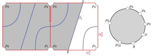
Figure 6. A split curve and a composite boundary degeneration. Right: the decorated source of a holomorphic curve. Left: its image. The end of the slit is a boundary branch point. As the slit shrinks to zero, the curve degenerates a split curve with $e\infty$ asymptotics $\rho_{3}$ and $\rho_{4}$ and $w\infty$ asymptotic $\rho_{34}$; this is a collision end. As the slit approaches the chord $\rho_{12}$ the curve degenerates a composite boundary degeneration (a boundary degeneration and a join curve).

Figure 7. A two-story end and a simple boundary degeneration. When the slit gets long, approaching the left edge, the curve degenerates to a 2-story holomorphic building. When the slit shrinks to zero, the curve becomes a simple boundary degeneration.

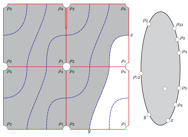
Figure 8. An orbit curve end and a collision end. When the slit approaches the puncture, an orbit curve degenerates. When the slit shrinks to zero, a split curve degenerates.

3.2. Definitions of the moduli spaces

In this subsection, we will define the moduli spaces of holomorphic curves used later in the paper. Briefly, these are:

1. The moduli spaces of curves in $\bigl{(}\Sigma\times[0,1]\times\mathbb{R},({\boldsymbol{\alpha}}\times\{1\}\times\mathbb{R})\cup({\boldsymbol{\beta}}\times\{0\}\times\mathbb{R})\bigr{)}$ with a fixed source. These are denoted $\mathcal{M}^{B}(\mathbf{x},\mathbf{y};{S^{\mspace{1.0mu}\triangleright}})$ where $\mathbf{x}$ and $\mathbf{y}$ are generators, $B$ is a homology class, and ${S^{\mspace{1.0mu}\triangleright}}$ is a decorated Riemann surface.

2. The moduli spaces of embedded curves in $\bigl{(}\Sigma\times[0,1]\times\mathbb{R},({\boldsymbol{\alpha}}\times\{1\}\times\mathbb{R})\cup({\boldsymbol{\beta}}\times\{0\}\times\mathbb{R})\bigr{)}$. These are denoted $\mathcal{M}^{B}(\mathbf{x},\mathbf{y};\vec{a};w)$ where $\vec{a}$ is a sequence of basic algebra elements and $w\in\mathbb{Z}_{\geq 0}$ is the number of orbits.

3. The moduli spaces of holomorphic curves in $\bigl{(}\mathbb{R}\times\partial\Sigma\times[0,1]\times\mathbb{R},{\boldsymbol{\alpha}}\times\{1\}\times\mathbb{R}\bigr{)}$ with a fixed source, i.e., curves at $e\infty$. These are denoted $\mathcal{N}(T^{\mspace{1.0mu}\rotatebox{90.0}{$\scriptstyle\lozenge$}})$.

4. The moduli spaces of curves in $\bigl{(}\Sigma\times\mathbb{H},{\boldsymbol{\alpha}}\times\{1\}\times\mathbb{R}\bigr{)}$ with a fixed source (where $\mathbb{H}=(-\infty,1]\times\mathbb{R}$). These are denoted $\mathcal{N}(\mathbf{x};S^{\mspace{1.0mu}{\Box}})$ or $\mathcal{N}(*;S^{\mspace{1.0mu}{\Box}})$ depending on whether the asymptotics at $\infty$ in $\mathbb{H}$ are fixed or allowed to vary.

5. The moduli spaces of embedded curves in $\bigl{(}\Sigma\times\mathbb{H},{\boldsymbol{\alpha}}\times\{1\}\times\mathbb{R}\bigr{)}$. These are denoted $\mathcal{N}(\mathbf{x};\vec{a};w)$ or $\mathcal{N}(*;\vec{a};w)$, again depending on whether the asymptotics at $\infty$ are fixed or not. (A variant $\mathcal{N}([\alpha_{i}^{a}];\vec{a};w)$ is introduced in Section 3.5.) Again, $\vec{a}$ is a sequence of basic algebra elements.

Properties of these moduli spaces are developed in later subsections. For the construction of $\widehat{\mathit{CFA}}$ and $\widehat{\mathit{CFD}}$, we do not use directly the moduli spaces with a fixed source; rather, those are used as auxiliary steps in understanding the moduli spaces of embedded curves. Types (1), (2), and (3) are generalizations of moduli spaces considered for bordered $\widehat{\mathit{HF}}$ [LOT18, Chapter 5]; Types (4) and (5) are analogues of boundary degenerations or disk bubbles (see, e.g., [FOOO09], and also [OZ11]).

Before turning to the construction of the moduli spaces themselves, we describe the kinds of almost complex structures we will use.

3.2.1. Families of almost complex structures

Difficulties with transversality force us to use somewhat more intricate families of almost complex structures than for the case of $\widehat{\mathit{HF}}$. In this section, we specify the compatibility conditions those families are required to satisfy. We will define two notions:

• An “$\eta$-admissible almost complex structure” (Definition 3.4). This spells out the conditions a single almost complex structure is required to satisfy.

• A “coherent family of $\eta$-admissible almost complex structures” (Definition 3.6). This spells out the compatibility conditions for families of almost complex structures needed to define points in our moduli spaces which, in turn, are used to define the operations $m_{1+n}^{w}$.

Transversality conditions for those families are deferred to Section 3.5; a coherent family of almost complex structures which is also sufficiently generic for counting curves will be called a “tailored family” (Definition 3.51). For technical reasons, we will not be able to work with a single almost complex structure for all moduli spaces.

A key ingredient in these definitions is a particular moduli space of marked polygons:

Definition 3.1.

A bimodule component is a conformal disk with $n\geq 2$ boundary marked points and some number of interior marked points, a choice of two distinguished boundary marked points called $\pm\infty$, and a function from the other marked points to $\mathbb{Z}_{>0}$, called the energy, so that the energy of each interior marked point is a multiple of $4$. We require that there be at least one marked point other than $\pm\infty$.

Forgetting all of the marked points except $\pm\infty$ induces an identification of the disk minus $\{\pm\infty\}$ with $[0,1]\times\mathbb{R}$, well-defined up to translation. Under this identification, the boundary of the disk is divided into two parts, which we refer to as $\{0\}\times\mathbb{R}$ and $\{1\}\times\mathbb{R}$. The energies of the boundary marked points on $\{1\}\times\mathbb{R}$ (respectively $\{0\}\times\mathbb{R}$) defines a sequence $\vec{E}$ (respectively $\vec{E}^{\prime}$). Call the marked points labeled by $\pm\infty$ the module vertices, the marked points on $\{0\}\times\mathbb{R}$ the left algebra vertices, and the marked points on $\{1\}\times\mathbb{R}$ the right algebra vertices.

Given a pair of non-negative integers $(k,\ell)$, sequences of positive integers $\vec{E}^{\prime}=(E^{\prime}_{1},\dots,E^{\prime}_{k})$ and $\vec{E}=(E_{1},\dots,E_{\ell})$, and a non-negative integer $w$, let $\mathfrak{M}_{k,\ell,\vec{E^{\prime}},\vec{E},w}$ be a copy of the associaplex ${\mathbf{X}}^{k+1+\ell,w}$. We think of $\mathfrak{M}_{k,\ell,\vec{E^{\prime}},\vec{E},w}$ as a compactification of the space of module polygons with $k$ vertices on $\{0\}\times\mathbb{R}$, $\ell$ vertices on $\{1\}\times\mathbb{R}$, total energy of interior punctures $4w$, and energies of the boundary punctures specified by $\vec{E}^{\prime}$ and $\vec{E}$.

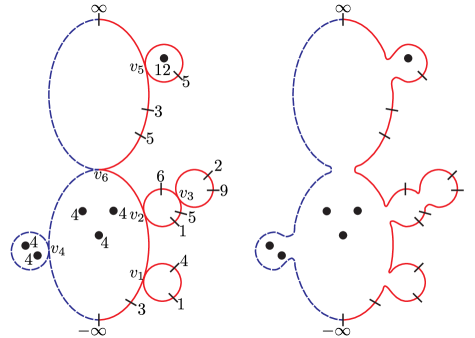
Figure 9. A bimodule polygon $x$ (left) and its gluing $\widetilde{x}$ (right). The left boundary is dashed and the right boundary is solid. Disks in $x$ whose boundary is entirely solid are left algebra-type components, disks whose boundary is entirely dashed are right algebra-type components, and the two disks with both dashed and solid boundaries are bimodule components. The energies of the nodes $v_{1},\dots,v_{5}$ are $5$, $23$, $11$, $8$, and $17$, respectively. The node $v_{6}$ is not assigned an energy.

By definition, a point $x\in\mathfrak{M}_{k,\ell,\vec{E^{\prime}},\vec{E},w}$ is a tree of disks meeting at nodes. We can glue the disks in $x$ together at the nodes to obtain a single disk $\widetilde{x}$. (See Figure 9.) The identification between the boundary of $x$ and $\widetilde{x}$ identifies the arcs in the boundary of each disk in $x$ with a subset of either $\{0\}\times\mathbb{R}$ or $\{1\}\times\mathbb{R}$. Call a disk in $x$ a left algebra-type component if its whole boundary corresponds to a subset of $\{0\}\times\mathbb{R}$, a right algebra-type component if its whole boundary corresponds to a subset of $\{1\}\times\mathbb{R}$, and a bimodule-type component otherwise. Suppose $v$ is a node of $x$ so that at least one of the disks meeting at $v$ is a (left or right) algebra-type component. Cutting $x$ at $v$ gives two trees of disks, one of which consists entirely of algebra-type components. Define the energy of $v$ to be sum of the energies of the marked points (not nodes) of that tree of algebra-type components. With this definition, each bimodule-type component in $x$ is a bimodule component.

Let $\mathfrak{M}$ be the disjoint union of all the $\mathfrak{M}_{k,\ell,\vec{E}^{\prime},\vec{E},w}$ and, given a positive integer $E$, let $\mathfrak{M}_{E}$ be the disjoint union of all $\mathfrak{M}_{k,\ell,\vec{E^{\prime}},\vec{E},w}$ so that $E^{\prime}_{1}+\cdots+E^{\prime}_{k}+E_{1}+\cdots+E_{\ell}+4w=E$. We call a point in $\mathfrak{M}$ a bimodule polygon. In particular, a bimodule component is a special case of a bimodule polygon.

We can also define a notion of module polygons: a module polygon is an element of $\mathfrak{M}_{0,n,,\vec{E},w}$ for some $n$, $\vec{E}$, and $w$. (A module component is a module polygon with a single component.) However, some components of a module polygon may be bimodule components, because algebra-type components can bubble off along $\{0\}\times\mathbb{R}$.

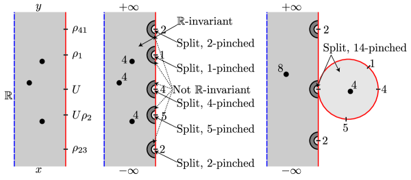
Figure 10. Polygons and almost complex structures. Left: a moduli space of curves we will consider, corresponding to a term $m_{6}^{3}(x,\rho_{23},U\rho_{2},U,\rho_{1},\rho_{41})=y$. Center: a corresponding module polygon and the conditions on an $\eta$-admissible almost complex structure for that module polygon. In the figure, $n$-pinched means $\eta(n)$-pinched. Right: a degeneration of such a module polygon, where two interior marked points come together and a disk bubbles off the boundary, together with the conditions imposed on a corresponding almost complex structure.

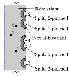
Figure 11. Polygons and almost complex structures, continued. If $\delta$ is larger than a quarter the distance between two of the algebra marked points, the various disks in Condition (J-4) are not disjoint.

A second ingredient to specify the complex structures we will consider is a pinching function and a pinched almost complex structure. (The two notions come together in Definition 3.4.)

Definition 3.2.

A pinching function is a monotone-decreasing function $\eta\nobreak\mskip 2.0mu\mathpunct{}\nonscript\mkern-3.0mu{:}\penalty 300\mskip 6.0mu plus 1.0mu\mathbb{Z}_{>0}\to\mathbb{R}_{>0}$.

Definition 3.3.

Fix, once and for all, a small positive number $\delta_{0}$. Given another real number $\epsilon>0$, call a complex structure $j$ on $\Sigma$ $\epsilon$-pinched if:

1. There is a circle $C\subset\Sigma\setminus{\boldsymbol{\alpha}}$ separating $\alpha_{1}^{a}\cup\alpha_{2}^{a}$ from $\alpha_{1}^{c}\cup\cdots\cup\alpha_{g-1}^{c}$ which has a neighborhood disjoint from the $\alpha$-curves biholomorphic to $\{z\in\mathbb{C}\mid 1<|z|<1/\epsilon\}$.

2. There is no essential circle in the component of $\Sigma\setminus C$ containing $\alpha_{1}^{a}\cup\alpha_{2}^{a}$ which has a neighborhood biholomorphic to $\{z\in\mathbb{C}\mid 1<|z|<1/\delta_{0}\}$.

(Later, we will sometimes consider limits as $\epsilon\to 0$. The second bullet point is to ensure that no other curves in this component of $\Sigma\setminus C$ collapse in the result.)

Since we are pinching a specified isotopy class of curves $C$, the space of $\epsilon$-pinched complex structures on $\Sigma$ is contractible.

We are now ready to turn to the conditions on our almost complex structures.

Definition 3.4.

Fix a pinching function $\eta$ and a bimodule component $P$ with $n$ right algebra vertices. Recall that there is an identification of $P$ with $[0,1]\times\mathbb{R}$, well-defined up to translation. An almost complex structure $J$ on $\Sigma\times P$ is $\eta$-admissible if it satisfies the following conditions.

1. The projection map $\pi_{P}\nobreak\mskip 2.0mu\mathpunct{}\nonscript\mkern-3.0mu{:}\penalty 300\mskip 6.0mu plus 1.0mu\Sigma\times P\to P$ is $J$-holomorphic.

2. Thinking of $P$ as $[0,1]\times\mathbb{R}$, if $\partial/\partial s$ and $\partial/\partial t$ are the vector fields generating translation in $[0,1]$ and $\mathbb{R}$, respectively, $J(\partial/\partial s)=\partial/\partial t$.

3. There is a neighborhood $D$ of the puncture in $\Sigma$ so that the almost complex structure $J$ splits as $j_{\Sigma}\times j_{P}$ over $D\times P\subset\Sigma\times P$. Also, $J$ splits as $j_{\Sigma}\times j_{P}$ over some neighborhood of $\{0\}\times\mathbb{R}$.

4. Let $(1,t_{1}),\dots,(1,t_{n})$ be the images of the right algebra vertices under some holomorphic identification of $P$ with $[0,1]\times\mathbb{R}$. (The $t_{i}$ are well-defined up to an overall translation.) Then, there is some $0<\delta<1/2$ so that:

   1. outside the balls of radius $2\delta$ around the $(1,t_{i})$, $J$ is invariant under (small) translations in $\mathbb{R}$, and

   2. inside the ball of radius $\delta$ around $(1,t_{i})$, $J$ is split as $j_{i}\times j_{P}$, for some complex structure $j_{i}$ on $\Sigma$.

5. If $E_{i}$ is the energy of the $i^{\text{th}}$ marked point of $P$ then $j_{i}$ is $\eta(E_{i})$-pinched.

We extend this definition to the boundary of $\mathfrak{M}$ as follows. Consider a boundary point $P$ of $\mathfrak{M}$, consisting of some bimodule components and some algebra components. By an $\eta$-admissible almost complex structure $J$ over such a configuration we mean an $\eta$-admissible almost complex structure in the sense above over each of the bimodule components, so that these agree near $\pm\infty$ in the obvious sense (using Condition (J-4)(J-4)(a)). The almost complex structures on the bimodule components determine an almost complex structure on $\Sigma\times P_{0}$ for each algebra-type component $P_{0}$ of $P$ by condition (J-4)(J-4)(b): we simply require the complex structure to be split as $j_{i}\times j_{P_{0}}$, if $P_{0}$ is attached at the $i^{\text{th}}$ marked point on the right, or as $j_{\Sigma}\times j_{P_{0}}$ if $P_{0}$ is attached at a marked point on the left.

In particular, Conditions (J-1) and (J-2) imply that we can (and often will) view $J(P)$ as a family of complex structures on $\Sigma$, parameterized by $P$. Condition (J-4)(J-4)(a) implies that $J$ has a well-defined asymptotic behavior at $\pm\infty$: near $\pm\infty$, $J$ is specified by a 1-parameter family of almost complex structures $j_{s}$, $s\in[0,1]$, on $\Sigma$. (By condition (J-3), $j_{s}=j_{\Sigma}$ near $s=0$.)

Figures 10 and 11 give schematics of what Conditions (J-4) and (J-5) require.

We make the space of $\eta$-admissible almost complex structures into a bundle over $\mathfrak{M}$ as follows. Over the top stratum of $\mathfrak{M}$, the definition of this bundle is clear, using the $C^{\infty}$ topology on the space of endomorphisms of $T(\Sigma\times[0,1]\times\mathbb{R})$, say. Next, suppose $P$ is a boundary point of $\mathfrak{M}$, and that $\operatorname{glue}(P)$ is obtained by gluing together the components of $P$ (with small gluing parameter $\epsilon$, say). Because the almost complex structures are split near the marked points, the $\eta$-admissible almost complex structure over $P$ induces an $\eta$-admissible almost complex structure $\operatorname{glue}(J)$ over $\operatorname{glue}(P)$. Then, for each triple of positive real numbers $\delta$, $\delta^{\prime}$, and $\epsilon$ and open neighborhood $V$ of $J$, we declare there to be a basic open neighborhood $V$ of $J$ consisting of those $J^{\prime\prime}$ which agree with $\operatorname{glue}(J^{\prime})$ on a disk of radius $\delta$ around the algebra marked points and are within distance $\delta^{\prime}$ of $\operatorname{glue}(J^{\prime})$ in the $C^{\infty}$ topology everywhere, for some $J^{\prime}\in V$ and gluing parameter $\epsilon^{\prime}<\epsilon$. (Here, as in Definition 3.4, distances are measured with respect to the identification of $\operatorname{glue}(P)$ and the bimodule components of $P$ with $[0,1]\times\mathbb{R}$.)

Lemma 3.5.

The fibers of the projection from the space of $\eta$-admissible almost complex structures projects to $\mathfrak{M}$ are contractible.

Proof.

Fix a point $P$ in $\mathfrak{M}$; without loss of generality, we may assume that $P$ is in the interior of $\mathfrak{M}$, i.e., consists of a single bimodule component. Let $\mathcal{J}$ denote the space of almost complex structures as in Definition 3.4 for $P$.

Fix a single curve $C$ representing the isotopy class where the pinching occurs. There is a subspace of $\mathcal{J}_{0}$ of $\mathcal{J}$ where the pinching occurs along $C$. The inclusion $\mathcal{J}_{0}\hookrightarrow\mathcal{J}$ is a homotopy equivalence, so it suffices to show that $\mathcal{J}_{0}$ is contractible.

A key notion we will use is that of a collar. Given a number $\delta\in(0,1/2)$, let $F_{\delta}$ be the union of the closed balls of radius $\delta$ around the $t_{i}$ and $G_{\delta}$ the complement of the union of the open balls of radius $2\delta$ around the $t_{i}$. By construction, $F_{\delta}$ and $G_{\delta}$ are closed and at distance $d(F_{\delta},G_{\delta})=\delta$ from each other. By a $(\delta_{1},\delta_{2})$-collar we mean a union of strips in $([0,1]\times\mathbb{R})\setminus(F_{\delta_{1}}\cup G_{\delta_{2}})$ separating $F_{\delta_{1}}$ from $G_{\delta_{2}}$. Such a collar exists as long as $F_{\delta_{1}}\cap G_{\delta_{2}}=\emptyset$.

Let $E=\max\{E_{1},\dots,E_{n}\}$.

There is a subspace $\mathcal{J}_{1}\subset\mathcal{J}_{0}$ so that on each disk around $(1,t_{i})$, $J$ is $\eta(E)$-pinched rather than just $\eta(E_{i})$-pinched as in Condition (J-5). That is, $J$ is $\eta(E)$-pinched on all of $F_{\delta}$. The inclusion $\mathcal{J}_{1}\hookrightarrow\mathcal{J}_{0}$ is a homotopy equivalence. (One can see this by deforming $\mathcal{J}_{0}$ into $\mathcal{J}_{1}$ by pinching more along $C$, using a collar.)

For each $\delta\in(0,1/2)$, let $\mathcal{J}_{1,\delta}$ be the subspace of $\mathcal{J}_{1}$ defined using the parameter $\delta$. Contractibility of the space of almost complex structures on $\Sigma$ compatible with a given area form implies that each $\mathcal{J}_{1,\delta}$ is contractible.

Finally, to see that $\mathcal{J}_{1}$ is contractible, suppose that $\delta_{1}$ and $\delta_{2}$ are close enough that there is a $(\delta_{1},\delta_{2})$-collar. Fix such a collar. Then the subspace of $\mathcal{J}_{1}$ of almost complex structures which vary only over the collar (i.e., satisfy either Condition (J-4)(J-4)(a) or (J-4)(J-4)(b) outside the collar) is contractible (for the same reason $\mathcal{J}_{1,\delta}$ is) and includes into $\mathcal{J}_{1,\delta_{1}}$, $\mathcal{J}_{1,\delta_{2}}$, and $\mathcal{J}_{1,\delta_{1}}\cap\mathcal{J}_{1,\delta_{2}}$ as homotopy equivalences. So, it follows by an inductive argument that the union $\mathcal{J}_{1}=\bigcup_{\delta}\mathcal{J}_{1,\delta}$ is also contractible. ∎

We will often shorthand Lemma 3.5 by saying that the space of $\eta$-admissible almost complex structures is contractible.

Definition 3.6.

Fix a pinching function $\eta$. A coherent family of $\eta$-admissible almost complex structures is a continuous section of the bundle of $\eta$-admissible almost complex structures (over $\mathfrak{M}$) satisfying the following compatibility conditions:

1. All of the almost complex structures agree near $\pm\infty$, i.e., they all correspond to the same 1-parameter family of complex structures $j_{s}$, $s\in[0,1]$, on $\Sigma$. We will sometimes write $J_{\infty}$ for the $\mathbb{R}$-invariant almost complex structure on $\Sigma\times[0,1]\times\mathbb{R}$ corresponding to this path $j_{s}$.

2. If $P$ is in the boundary of $\mathfrak{M}$ and $P^{\prime}$ is a bimodule component of $P$, then the restriction of $J(P)$ to $P^{\prime}$ agrees with $J(P^{\prime})$.

Note that we do not require any compatibility on the algebra-type components. (It will turn out that the counts of holomorphic curves corresponding to these components are independent of the complex structure, by Theorem 4.3.)

Lemma 3.7.

For any pinching function $\eta$, a coherent family $J$ of $\eta$-admissible almost complex structures exists.

Proof.

The proof is an induction on the total energy. First, fix any translation-invariant almost complex structure $J_{\infty}$ on $\Sigma\times[0,1]\times\mathbb{R}$. We will require that all of the $\eta$-admissible almost complex structures $J(P)$ agree with $J_{\infty}$ outside a neighborhood of their algebra punctures. Suppose we have constructed $J(P)$ for all polygons $P$ with energy $<E_{0}$ and consider the space of polygons with energy $E_{0}$. Fix some $\eta(E_{0})$-pinched almost complex structure on $\Sigma$; we will require that almost complex structures agree with this one near punctures with energy $E_{0}$. (This only occurs when the polygon has a single bimodule component and that component has a single algebra puncture, with energy $E_{0}$, and no interior punctures.) In particular, if $P$ has no algebra punctures and no punctures, $J(P)$ is given by $J_{\infty}$.

The family $J$ is already defined on the subspace of $\mathfrak{M}_{E_{0}}$ consisting of trees of disks where at least two of the components are bimodule components, because each of these components is in $\mathfrak{M}_{E}$ for some $E<E_{0}$ and on all algebra-type components $J$ is required to be constant. We extend $J$ to the strata where there is a single bimodule polygon inductively on the number of interior punctures and, for each number of interior punctures, inductively on the number of boundary punctures. Suppose we have constructed $J$ for all bimodule components with $<m$ interior punctures and with $m$ interior punctures and $<n$ boundary punctures. We will discuss the induction increasing $n$; increasing $m$ is similar. (Though it is not needed here, note that $n$ and $m$ are bounded in terms of $E_{0}$.)

Each point $P$ in the boundary of the subspace of $\mathfrak{M}_{E_{0}}$ with $m$ interior punctures and $n$ boundary punctures is a tree of bimodule and algebra-type components where each bimodule component is earlier in the induction. So, we have already defined the almost complex structure on $\Sigma\times P$ or, equivalently, the family of complex structures on $\Sigma$ parameterized by $P$. Further, if there is more than one bimodule component in $P$, the chosen almost complex structures for those components agree with the ones chosen before for $E<E_{0}$. A neighborhood of $P$ is given by gluing together the components of $P$ at the nodes, with various parameters. Given some $\delta>0$ and a gluing $\tilde{P}$ of $P$ small enough that all punctures on the same algebra-type component of $P$ lie within $\delta$ of each other in $\tilde{P}$, define the complex structures in $\delta$-neighborhoods of the punctures of $\tilde{P}$ to agree with the corresponding complex structure at the puncture of $P$, and choose interpolating complex structures for the regions between $\delta$-neighborhoods and $2\delta$-neighborhoods. Making these choices consistently across the different boundary strata defines $J$ in a neighborhood of the boundary of $\mathfrak{M}_{E_{0}}$. (Spelling out how to make such consistent choices takes some work, but is essentially the same as making consistent choices of strip-like ends in Floer theory [Sei08, Section (9g)].) Contractibility of the space of $\eta$-admissible almost complex structures guarantees we can then extend this family $J$ to all of $\mathfrak{M}_{E_{0}}$. ∎

To relate the above spaces of almost complex structures and the sequences of algebra elements used in the definitions of the $A_{\infty}$-operations, we use the notion of the energy of a sequence of algebra elements. Recall that a basic algebra element is an algebra element of the form $U^{i}\rho^{j}$ or $U^{i}\iota_{j}$, with those the first kind called Reeby elements. Define the energy of a basic algebra element to be $E(U^{i}\rho^{j})=4i+|\rho^{j}|$ and $E(U^{i}\iota_{j})=4i$, where $|\rho^{j}|$ denotes the length of $\rho^{j}$. More generally, given a sequence of basic algebra elements $\vec{a}$ and a non-negative integer $w$, define the energy of $(\vec{a},w)$ to be

(3.8) $$E(\vec{a},w)=4w+\sum E(a_{j}).$$

The definition is chosen so that

(3.9) $$E(\mu^{w}_{k}(a_{1},\dots,a_{k}),0)=E(a_{1},\dots,a_{k},w),$$

in the sense that each basic term in the sum on the left-hand side has the indicated energy.

Now, given a sequence $(a_{1},\dots,a_{m})$ of basic algebra elements and a non-negative integer $w$, there is a corresponding component of $\mathfrak{M}$ where the main stratum has $w$ interior marked points of weight $4$, no boundary marked points on $\{0\}\times\mathbb{R}$, and $m$ boundary marked points on $\{1\}\times\mathbb{R}$ labeled by the energies $E(a_{1}),\dots,E(a_{m})$ (in that order). Let $\mathfrak{M}(a_{1},\dots,a_{m};w)$ denote this component. Given an $\eta$-admissible family $J$ of almost complex structures, define

$$J(a_{1},\dots,a_{m};w)$$

to be the restriction of $J$ to $\mathfrak{M}(a_{1},\dots,a_{m};w)$. That is, $J(a_{1},\dots,a_{m};w)$ consists of an almost complex structure on $\Sigma\times P$ for each polygon $P\in\mathfrak{M}(a_{1},\dots,a_{m};w)$. See Figure 10.

3.2.2. Maps to $\Sigma\times[0,1]\times\mathbb{R}$

Fix a sequence of basic algebra elements $\vec{a}=(a_{1},\dots,a_{m})$ in the sense of Definition 1.8. Our moduli spaces will depend on this sequence: the underlying chord sequence (in the sense of Definition 1.8) specifies the asymptotics of the holomorphic curves, while the whole sequence of basic algebra elements will specify a family of almost complex structures as in Section 3.2.1.

Fix a pinching function $\eta$ and a coherent family $J$ of $\eta$-admissible almost complex structures.

As we did for $\widehat{\mathit{HF}}$, we will encode the asymptotics of our holomorphic curves in terms of decorations of the source:

Definition 3.10.

A decorated source ${S^{\mspace{1.0mu}\triangleright}}$ is a smooth surface $S$ with boundary, interior punctures, and boundary punctures, together with:

1. A labeling of each interior puncture by a positive integer, its multiplicity, and

2. A labeling of each boundary puncture by either $-\infty$, $+\infty$, or a basic algebra element $a$.

We will refer to the boundary punctures labeled by algebra elements as algebra punctures. Sometimes it will be more convenient to talk about the ramification of an interior puncture, which is one less than its multiplicity. (The terminology is the same as for zeroes of holomorphic maps.)

A multiplicity $r$ Reeb orbit is a map $S^{1}\to\partial\Sigma\times[0,1]\times\mathbb{R}$ which maps to $[0,1]\times\mathbb{R}$ by a constant map and which winds around $\partial\Sigma$ $r$ times.

The following is the analogue of [LOT18, Definition 5.2]:

Definition 3.11.

Let ${S^{\mspace{1.0mu}\triangleright}}$ be a decorated source. We say a smooth map

(3.12) $$u\nobreak\mskip 2.0mu\mathpunct{}\nonscript\mkern-3.0mu{:}\penalty 300\mskip 6.0mu plus 1.0mu(S,\partial S)\to(\Sigma\times[0,1]\times\mathbb{R},{\boldsymbol{\alpha}}\times\{1\}\times\mathbb{R}\cup{\boldsymbol{\beta}}\times\{0\}\times\mathbb{R})$$

respects ${S^{\mspace{1.0mu}\triangleright}}$ if $u$ is proper and:

• at each interior puncture with multiplicity $r$, $u$ is asymptotic to a multiplicity $r$ Reeb orbit;

• at each boundary puncture labeled $-\infty$, $u$ is asymptotic to $x\times[0,1]\times\{-\infty\}$ for some $x\in{\boldsymbol{\alpha}}\cap{\boldsymbol{\beta}}$;

• at each boundary puncture labeled $+\infty$, $u$ is asymptotic to $y\times[0,1]\times\{+\infty\}$ for some $y\in{\boldsymbol{\alpha}}\cap{\boldsymbol{\beta}}$;

• at each boundary puncture labeled $U^{m}\rho$, $u$ is asymptotic to $\rho\times\{(1,t)\}$ for some $t\in\mathbb{R}$; and

• at each boundary puncture labeled $U^{m}\iota_{j}$, $u$ is asymptotic to a point $(x,1,t)$ where $x$ lies in the interior of the $\alpha$-arc corresponding to $\iota_{j}$. (In particular, these last punctures are removable singularities.)

Given a map $u$ as in Definition 3.11, where ${S^{\mspace{1.0mu}\triangleright}}$ has $n$ boundary punctures and $w$ interior punctures, $n+2w\geq 3$, projection to $[0,1]\times\mathbb{R}$ specifies a module polygon $P(u)\in\mathfrak{M}$ with $n$ vertices, the images of the punctures (as long as those images are distinct). The family $J$ then specifies a corresponding almost complex structure on $\Sigma\times[0,1]\times\mathbb{R}$, $J(P(u))$. In the special case that $n=2$ and $w=0$, $P(u)$ would be a bigon with no interior punctures, which we disallowed; in this case, let $J(P(u))$ be $J_{\infty}$, the $\mathbb{R}$-invariant almost complex structure that all the $J(P)$ agree with near $\pm\infty$.

The following is the analogue of [LOT18, Definition 5.3]:

Definition 3.13.

Given generators $\mathbf{x},\mathbf{y}\in\mathfrak{S}(\mathcal{H})$, a homology class $B\in\pi_{2}(\mathbf{x},\mathbf{y})$, and a decorated source ${S^{\mspace{1.0mu}\triangleright}}$, let $\widetilde{\mathcal{M}}^{B}(\mathbf{x},\mathbf{y};{S^{\mspace{1.0mu}\triangleright}})$ be the set of maps $u$ as in Formula (3.12) so that:

1. The map $u$ is $(j,J(P(u))$-holomorphic for some almost complex structure $j$ on $S$.

2. The map $u$ respects ${S^{\mspace{1.0mu}\triangleright}}$.

3. For each $t\in\mathbb{R}$ and each $i$, $u^{-1}(\beta_{i}\times\{(0,t)\})$ consists of exactly one point, $u^{-1}(\alpha^{c}_{i}\times\{(1,t)\})$ consists of exactly one point, and $u^{-1}(\alpha^{a}_{i}\times\{(1,t)\})$ consists of at most one point.

Let $\mathcal{M}^{B}(\mathbf{x},\mathbf{y};{S^{\mspace{1.0mu}\triangleright}})$ be the quotient of $\widetilde{\mathcal{M}}^{B}(\mathbf{x},\mathbf{y};{S^{\mspace{1.0mu}\triangleright}})$ by the action of $\mathbb{R}$ by translation.

Condition (M-3) is called strong boundary monotonicity. In particular, this condition implies that if $\mathcal{M}^{B}(\mathbf{x},\mathbf{y};{S^{\mspace{1.0mu}\triangleright}})\neq\emptyset$ then the algebra punctures, and hence the basic algebra elements labeling them, are ordered. (In particular, the images in $\{1\}\times\mathbb{R}$ of the algebra punctures are distinct, so $P(u)$ is defined.) Specifically, if we fill in the punctures of $S$ to obtain a surface $\overline{S}$ then there must be an arc in $\partial\overline{S}$ starting at a (filled-in) $-\infty$ puncture and ending at a (filled-in) $+\infty$-puncture, and containing all the algebra punctures. The boundary orientation orients that arc, and hence orders the algebra punctures. Thus, ${S^{\mspace{1.0mu}\triangleright}}$ specifies a list $(a_{1},\dots,a_{k})$ of basic algebra elements.

Definition 3.14.

Given generators $\mathbf{x},\mathbf{y}\in\mathfrak{S}(\mathcal{H})$, a sequence of basic algebra elements $\vec{a}$, a homology class $B\in\pi_{2}(\mathbf{x},\mathbf{y})$, and a non-negative integer $r$, let $\mathcal{M}^{B}(\mathbf{x},\mathbf{y};\vec{a};w,r)$ be the union over all decorated sources ${S^{\mspace{1.0mu}\triangleright}}$ of the set of $u\in\mathcal{M}^{B}(\mathbf{x},\mathbf{y};{S^{\mspace{1.0mu}\triangleright}})$ so that:

1. The map $u$ is an embedding.

2. If we list the algebra punctures of ${S^{\mspace{1.0mu}\triangleright}}$ according to the $\mathbb{R}$-coordinates $u$ sends them to, the corresponding sequence of algebra elements is $\vec{a}$.

3. The source ${S^{\mspace{1.0mu}\triangleright}}$ has $w$ interior punctures with total ramification $r$.

Let $\mathcal{M}^{B}(\mathbf{x},\mathbf{y};\vec{a};w)=\mathcal{M}^{B}(\mathbf{x},\mathbf{y};\vec{a};w,0)$.

The spaces $\mathcal{M}^{B}(\mathbf{x},\mathbf{y};\vec{a};w)$ will be used to define the modules $\mathit{CFA}^{-}_{nu}(\mathcal{H})$ and $\mathit{CFA}^{-}(\mathcal{H})$ and, indirectly, $\mathit{CFD}^{-}(\mathcal{H})$.

3.2.3. Maps to east infinity

Here we discuss the relevant holomorphic curves in $\mathbb{R}\times\partial\Sigma\times[0,1]\times\mathbb{R}$. The curves which appear are essentially the same as in the case of $\widehat{\mathit{HF}}$ [LOT18], except that chords can be longer, curves can also be asymptotic to orbits, and punctures labeled by $U^{m}\iota_{j}$ can collide with other punctures.

To shorten notation, write $Z=\partial\Sigma$. The manifold $\mathbb{R}\times Z\times[0,1]\times\mathbb{R}$ is non-compact in several directions; by far east $\infty$ we mean $\{\infty\}\times Z\times[0,1]\times\mathbb{R}$, and by west infinity we mean $\{-\infty\}\times Z\times[0,1]\times\mathbb{R}$.

Definition 3.15.

A bi-decorated source $T^{\mspace{1.0mu}\rotatebox{90.0}{$\scriptstyle\lozenge$}}$ is a smooth surface $T$ with boundary, interior punctures, boundary punctures, and boundary marked points, together with:

1. A labeling of each puncture by either $w\infty$ or $e\infty$,

2. A labeling of each interior puncture by a positive integer, its multiplicity,

3. A labeling of each boundary puncture by some Reeby algebra element, and

4. A labeling of each boundary marked point by some non-Reeby basic algebra element (i.e., of the form $U^{m}\iota_{j}$).

We require that the sum of the $U$-powers labeling the $w\infty$ punctures is equal to the sum of the $U$-powers labeling the $e\infty$ punctures plus the sum of the $U$-powers labeling the boundary marked points.

Definition 3.16.

Given a bi-decorated source $T^{\mspace{1.0mu}\rotatebox{90.0}{$\scriptstyle\lozenge$}}$, a smooth map

$$u\nobreak\mskip 2.0mu\mathpunct{}\nonscript\mkern-3.0mu{:}\penalty 300\mskip 6.0mu plus 1.0mu(T,\partial T)\to(\mathbb{R}\times Z\times[0,1]\times\mathbb{R},\mathbb{R}\times\mathbf{a}\times\{1\}\times\mathbb{R})$$

respects $T^{\mspace{1.0mu}\rotatebox{90.0}{$\scriptstyle\lozenge$}}$ if $u$ is proper and:

• The map $\pi_{\mathbb{D}}\circ u\nobreak\mskip 2.0mu\mathpunct{}\nonscript\mkern-3.0mu{:}\penalty 300\mskip 6.0mu plus 1.0muT\to[0,1]\times\mathbb{R}$ is constant, where $\pi_{\mathbb{D}}$ is projection from $\mathbb{R}\times Z\times[0,1]\times\mathbb{R}$ to the last two factors,

• At each interior puncture with multiplicity $r$, $u$ is asymptotic to a multiplicity $r$ Reeb orbit, at $\{-\infty\}\times Z$ if the puncture is labeled $w\infty$ and at $\{\infty\}\times Z$ if the puncture is labeled $e\infty$,

• At each boundary puncture labeled $(e\infty,U^{m}\rho)$, $u$ is asymptotic to $\{\infty\}\times\rho\times\{(1,t)\}$, while at each boundary puncture labeled $(w\infty,U^{m}\rho)$, $u$ is asymptotic to $\{-\infty\}\times\rho\times\{(1,t)\}$ (for some $t\in\mathbb{R}$), and

• Each boundary marked point labeled by $U^{m}\iota_{j}$ is mapped to a point on an element of $\mathbf{a}$ corresponding to $\iota_{j}$.

Let $\widetilde{\mathcal{N}}(T^{\mspace{1.0mu}\rotatebox{90.0}{$\scriptstyle\lozenge$}})$ denote the space of holomorphic maps $u$ which respect $T^{\mspace{1.0mu}\rotatebox{90.0}{$\scriptstyle\lozenge$}}$, and $\mathcal{N}(T^{\mspace{1.0mu}\rotatebox{90.0}{$\scriptstyle\lozenge$}})=\widetilde{\mathcal{N}}(T^{\mspace{1.0mu}\rotatebox{90.0}{$\scriptstyle\lozenge$}})/(\mathbb{R}\times\mathbb{R})$ denote the quotient of $\widetilde{\mathcal{N}}(T^{\mspace{1.0mu}\rotatebox{90.0}{$\scriptstyle\lozenge$}})$ by translation in the two $\mathbb{R}$ factors.

Note that a map $u$ as in Definition 3.16 is holomorphic if and only if its projection to $\mathbb{R}\times Z$ is holomorphic. Also, the sum of the energies of the $w\infty$ (boundary and interior) punctures is equal to the sum of the energies of the $e\infty$ punctures and the boundary marked points.

We will see later that, in codimension $1$, only four kinds of curves at $e\infty$ show up:

1. Split curves, as defined in [LOT18]. This is the case that $T$ consists of a single disk with three boundary punctures, two labeled $e\infty$ and one labeled $w\infty$, and no interior punctures. If the $e\infty$ boundary punctures are labeled $a$ and $b$ then the $w\infty$ puncture by the product $ab$. Reading counterclockwise around the boundary, the cyclic ordering of these punctures is $(a,b,ab)$. See Figure 13, left.

2. Join curves, also as defined in [LOT18]. This is the case that $T$ consists of a single disk with three boundary punctures, two labeled $w\infty$ and one labeled $e\infty$, and no interior punctures. The $w\infty$ boundary punctures are labeled $a$ and $b$, and the $e\infty$ puncture by the concatenation $ab$. Reading counterclockwise around the boundary, the cyclic ordering of these punctures is $(b,a,ab)$. Further, these occur only as parts of composite boundary degenerations (described below).

3. Orbit curves, which are new. The surface $T$ is a disk with one boundary puncture, labeled by $w\infty$ and some length-4 Reeb chord, and one interior puncture labeled $e\infty$ and multiplicity $1$. The corresponding map to $\mathbb{R}\times Z$ is a degree-1 branched cover, with a single boundary branch point. (The whole boundary is mapped to a ray on one component of $\mathbb{R}\times\mathbf{a}$, going out to $-\infty$, i.e., west infinity.) See Figure 12.

4. Pseudo split curves, consisting of a single disk with two boundary punctures, one labeled $(e\infty,U^{m}\rho)$ and the other $(w\infty,U^{m+n}\rho)$, and a boundary marked point labeled $U^{n}\iota_{j}$; see Figure 13, center. (These correspond to a puncture labeled by $U^{m}\rho$ colliding with a puncture labeled $U^{n}\iota_{j}$.)

Figure 12. An orbit curve. The source is drawn on the left; the map to $\mathbb{R}\times Z$ is indicated on the right.

Figure 13. A split curve, a pseudo split curve, and a fake split curve. Left: the image of a split curve in $\mathbb{R}\times Z$, with boundary $(a,b,ab)=(\rho_{1},\rho_{2},\rho_{12})$. Center: the image of a pseudo-split curve in $\mathbb{R}\times Z$. Right: the source of a fake split curve; this curve is mapped to $\Sigma\times[0,1]\times\mathbb{R}$ by a constant map.

It will be convenient to view one more kind of curve as a kind of degenerate case of an $e\infty$ curve:

1. Fake split curves consist of a disk with three boundary marked points (or punctures), labeled $U^{m}\iota_{j}$, $U^{n}\iota_{j}$, and $U^{m+n}\iota_{j}$, mapped to $\Sigma\times[0,1]\times\mathbb{R}$ by a constant map to some point $(x,1,t)$ where $x$ lies in the interior of the $\alpha$-arc corresponding to $\iota_{j}$. See Figure 13, right.

3.2.4. Boundary degenerations

Let $\mathbb{H}$ denote the half plane

(3.17) $$\mathbb{H}=(-\infty,1]\times\mathbb{R}=\{x+iy\mid x\leq 1\}\subset\mathbb{C},$$

with $\partial\mathbb{H}=\{1\}\times\mathbb{R}$. Let $\overline{\mathbb{H}}$ denote the one-point compactification of $\mathbb{H}$, which is just a disk.

As usual, we fix a complex structure $j$ on $\Sigma$. Boundary degenerations are holomorphic maps from a surface $S$ to the space $\Sigma\times\mathbb{H}$, equipped with the product complex structure $J$, which is $j$ on the $\Sigma$ factor and the usual complex structure $\mathbb{H}$ on the second. (In Section 4, we consider boundary degenerations using a more general class of almost complex structure on $\Sigma\times\mathbb{H}$.)

We start by defining a general boundary degeneration, which is needed for the compactness statement in Section 3.7. We then specialize to the kinds of boundary degenerations that occur in codimension $1$: simple boundary degenerations and composite boundary degenerations.

Definition 3.18.

A boundary degeneration source $S^{\mspace{1.0mu}{\Box}}$ consists of:

1. A surface-with-boundary $S$ with interior and boundary punctures,

2. A labeling of each interior puncture by a positive integer (which will be the multiplicity of the Reeb orbit), and

3. A labeling of each boundary puncture by a basic algebra element.

We will call the interior punctures and the boundary punctures labeled by elements $U^{m}\rho$ east punctures and the boundary punctures labeled by elements $U^{m}\iota_{j}$ removable punctures.

A map

$$u\nobreak\mskip 2.0mu\mathpunct{}\nonscript\mkern-3.0mu{:}\penalty 300\mskip 6.0mu plus 1.0mu(S,\partial S)\to(\Sigma\times\overline{\mathbb{H}},{\boldsymbol{\alpha}}\times\partial\overline{\mathbb{H}})$$

respects $S^{\mspace{1.0mu}{\Box}}$ if it satisfying the following conditions:

1. At each interior puncture with multiplicity (label) $r$, $u$ is asymptotic to a multiplicity $r$ Reeb orbit.

2. At each boundary puncture $q$ labeled by $U^{m}\rho$, $u$ is asymptotic to $\rho\times\{(1,t_{q})\}$ for some $t_{q}\in\mathbb{R}\cup\{\infty\}$.

3. At each boundary puncture $q$ labeled by $U^{m}\iota_{j}$, $u$ is asymptotic to $x\times\{(1,t_{q})\}$ for some $x$ in the $\alpha$-arc corresponding to $q$ and some $t_{q}\in\mathbb{R}\cup\{\infty\}$.

4. Exactly one $t_{q}$ is equal to $\infty$. Denote this $q$ by $q_{\infty}$.

5. For each $t\in\mathbb{R}$ which is not one of the $t_{q}$ and each $i=1,\dots,g-1$, $\overline{u}^{-1}(\alpha_{i}^{c}\times(1,t))$ consists of exactly one point and $u^{-1}((\alpha_{1}^{a}\cup\alpha_{2}^{a})\times(1,t))$ consists of exactly one point. (This condition is called boundary monotonicity.)

6. The energy of the label of $q_{\infty}$ is the sum of the energies of the labels of the other punctures (including the interior punctures). (This is a constraint on the power of $U$ in the label of $q_{\infty}$.)

Let $\widetilde{\mathcal{N}}(*;S^{\mspace{1.0mu}{\Box}})$ be the moduli space of maps $u$ respecting $S^{\mspace{1.0mu}{\Box}}$ which are $(j_{S},J)$-holomorphic with respect to some complex structure $j_{S}$ on $S$. Let $\mathcal{N}(*;S^{\mspace{1.0mu}{\Box}})$ be the quotient of $\widetilde{\mathcal{N}}(*,S^{\mspace{1.0mu}{\Box}})$ by translation and scaling on $\mathbb{H}$ (i.e., $(x,s,t)\mapsto(x,a(s-1)+1,at+b)$ for $a\in\mathbb{R}_{>0}$ and $b\in\mathbb{R}$).

For each boundary puncture $q$ there is an evaluation map

$$\operatorname{ev}_{q}\nobreak\mskip 2.0mu\mathpunct{}\nonscript\mkern-3.0mu{:}\penalty 300\mskip 6.0mu plus 1.0mu\mathcal{N}(*;S^{\mspace{1.0mu}{\Box}})\to(\alpha_{1}^{a}\cup\alpha_{2}^{a}\cup\{p\})\times\alpha_{1}^{c}\times\cdots\times\alpha_{g-1}^{c}$$

defined by

$$\operatorname{ev}_{q}(u)=(\pi_{\Sigma}\circ u)\bigl{(}(\pi_{\mathbb{H}}\circ u)^{-1}(t_{q})\bigr{)}.$$

We have $p\in\operatorname{ev}_{q}(u)$ if and only if $q$ is labeled by a Reeby element. The evaluation map corresponding to $q_{\infty}$ (the puncture mapped to $\infty$) will come up most frequently, so let

$$\operatorname{ev}=\operatorname{ev}_{q_{\infty}}.$$

Given $\mathbf{x}\in(\alpha_{1}^{a}\cup\alpha_{2}^{a}\cup\{p\})\times\alpha_{1}^{c}\times\cdots\times\alpha_{g-1}^{c}$, let

$$\mathcal{N}(\mathbf{x};S^{\mspace{1.0mu}{\Box}})=\operatorname{ev}^{-1}(\mathbf{x})\subset\mathcal{N}(*;S^{\mspace{1.0mu}{\Box}}).$$

If $\mathbf{x}$ has the form $\{p,y_{1},\dots,y_{g-1}\}$, so $q_{\infty}$ is labeled $U^{m}\rho$, we will also write $\mathcal{N}(\mathbf{x};S^{\mspace{1.0mu}{\Box}})$ as $\mathcal{N}(\rho\times\mathbf{y};S^{\mspace{1.0mu}{\Box}})$ where $\mathbf{y}=\{y_{1},\dots,y_{g-1}\}$.

Given $S^{\mspace{1.0mu}{\Box}}$ and $u\in\widetilde{\mathcal{N}}(*;S^{\mspace{1.0mu}{\Box}})\neq\emptyset$, the orientation of $\partial\mathbb{H}$ gives an ordering $\vec{a}(S^{\mspace{1.0mu}{\Box}})=(a;a_{1},\dots,a_{m})$ of the algebra elements marking $S^{\mspace{1.0mu}{\Box}}$, where we declare that the algebra element $a$ labeling $q_{\infty}$ comes first. By Condition (BD-5), this ordering is independent of the choice of $u$.

In codimension-1, two types of configurations involving boundary degenerations can occur. So, we name them:

Definition 3.19.

A simple boundary degeneration source is a boundary degeneration source so that $q_{\infty}$ is labeled $U^{m}\iota_{j}$ and no other boundary puncture is labeled $U^{m}\iota_{j}$. A (possibly non-embedded) simple boundary degeneration is a holomorphic curve $u$ respecting a simple boundary degeneration source.

Let $\mathbf{x}$ be a $g$-tuple of points in $(\alpha_{1}^{a}\cup\alpha_{2}^{a})\times\alpha^{c}_{1}\times\dots\times\alpha^{c}_{g-1}$, $\vec{a}$ be a sequence of Reeby algebra elements, and $w$ and $r$ be non-negative integers. Let $\mathcal{N}(\mathbf{x};\vec{a};w,r)$ be the set of pairs $(S^{\mspace{1.0mu}{\Box}},u)$ where $u$ is a simple boundary degeneration with source $S^{\mspace{1.0mu}{\Box}}$ such that

1. The map $u$ is an embedding.

2. The source $S^{\mspace{1.0mu}{\Box}}$ has $w$ interior punctures with total ramification $r$. (As above, the ramification of a puncture is one less than its multiplicity.)

3. The sequence of algebra element asymptotics of $u$ is $(U^{n};\vec{a})$ (for some appropriate $n$).

We will be particularly interested in the case $r=0$, so let

$$\mathcal{N}(\mathbf{x};\vec{a};w)=\mathcal{N}(\mathbf{x};\vec{a};w,0)$$

We call an element of $\mathcal{N}(\mathbf{x};\vec{a};w)$ a simple boundary degeneration based at $\mathbf{x}$.

Sometimes it will be more convenient not to fix the point $\mathbf{x}$; let

$$\mathcal{N}(*;\vec{a};w,r) =\bigcup_{\mathbf{x}}\mathcal{N}(\mathbf{x};\vec{a};w,r)$$

$$\mathcal{N}(*;\vec{a};w) =\bigcup_{\mathbf{x}}\mathcal{N}(\mathbf{x};\vec{a};w,0).$$

After discussing transversality, we will also consider another space $\mathcal{N}([\alpha_{i}^{a}];\rho^{1},\dots,\rho^{n};w)$ which is equal to $\mathcal{N}(\mathbf{x};\vec{\rho};w)$ for some generic $\mathbf{x}$ intersecting $\alpha_{i}^{a}$; see Section 3.5.

See Figure 14, left.

Definition 3.20.

A composite boundary degeneration source is a boundary degeneration source so that none of the punctures are labeled by elements of the form $U^{m}\iota_{j}$. A (possibly non-embedded) composite boundary degeneration is a triple $(S^{\mspace{1.0mu}{\Box}},u,v)$ where $S^{\mspace{1.0mu}{\Box}}$ is a composite boundary degeneration source, $u$ is a holomorphic curve respecting $S^{\mspace{1.0mu}{\Box}}$, and $v$ is a join curve, such that the Reeb chord $u$ is asymptotic to at $q_{\infty}$ is one of the $w\infty$ Reeb chords of $v$.

Let $\mathbf{x}$ be a $(g-1)$-tuple of points in $\alpha^{c}_{1}\times\dots\times\alpha^{c}_{g-1}$, $\vec{a}$ be a sequence of Reeby basic algebra elements, $b$ be another Reeby basic algebra element, and $w$ and $r$ be non-negative integers. Let $\mathcal{N}(b;a_{1},\dots,a_{n};w,r)$ denote the moduli space of composite boundary degenerations $(S^{\mspace{1.0mu}{\Box}},u,v)$ such that

1. The map $u$ is an embedding.

2. The source $S^{\mspace{1.0mu}{\Box}}$ has $w$ interior punctures with total ramification $r$.

3. Either:

   1. $u$ is asymptotic to $c$ at $\infty$ and to the sequence of Reeby basic algebra elements $(a_{1},\dots,a_{n-1})$ along $\{1\}\times\mathbb{R}$, $a_{n}=cb$ for some basic algebra element $c$, and $v$ is a join curve with asymptotics $(c,b)$ at $w\infty$ and $a_{n}$ at $e\infty$, or

   2. $u$ is asymptotic to $c$ at $\infty$ and to the sequence of Reeby basic algebra elements $(a_{2},\dots,a_{n})$ along $\{1\}\times\mathbb{R}$, $a_{1}=bc$, and $v$ is a join curve with asymptotics $(b,c)$ at $w\infty$ and $a_{1}$ at $e\infty$.

An element of $\mathcal{N}(b;a_{1},\dots,a_{n};w,r)$ is a composite boundary degeneration. In Point (BDc-3), the first case is called right-extended and the second case is called left-extended. As before, we are mostly interested in the case $r=0$ and will drop it from the notation in that case.

See Figure 14, right. Since there is a unique join curve asymptotic to chords $\sigma$, $\tau$, and $\sigma\tau$, the moduli space of composite boundary degenerations with given Reeb chords is in bijection with the space of maps $u$ as in Definition 3.20.

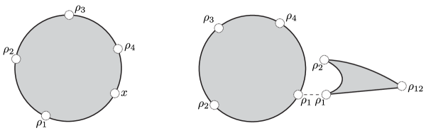
Figure 14. Sources for boundary degenerations. Left: the source for the simple boundary degeneration arising in Figure 7. The moduli space of embedded curves here is denoted $\mathcal{N}(\mathbf{x};\rho_{4},\rho_{3},\rho_{2},\rho_{1};0,0)$ where $\mathbf{x}$ is the point on the $\alpha$-arc labeled $x$ in Figure 7. Right: the source for the right-extended composite boundary degeneration arising in Figure 6. This moduli space is denoted $\mathcal{N}(\rho_{2};\rho_{4},\rho_{3},\rho_{2},\rho_{12};0,0)$. The join curve in Definition 3.20 has asymptotics $(\rho_{1},\rho_{2})$ at $w\infty$ and $\rho_{12}$ at $e\infty$. In the notation of Definition 3.20, $c=\rho_{1}$ and $b=\rho_{2}$.

Remark 3.21.

We will see in Section 4 that rigid, simple boundary degenerations (with inputs Reeb chords) correspond to centered operations on $\mathcal{A}_{-}$, and hence also to centered tiling patterns from [LOT21]. Composite boundary degenerations correspond to the left-extended and right-extended tiling patterns from [LOT21].

3.2.5. The tautological correspondence

For computing the index, it will be convenient to formulate certain of our holomorphic curves in terms of the symmetric product. Specifically, fix a coherent family of $\eta$-admissible almost complex structures, for some $\eta$. Consider a module polygon $P$ with a single component, and a $J(P)$-holomorphic map $u\nobreak\mskip 2.0mu\mathpunct{}\nonscript\mkern-3.0mu{:}\penalty 300\mskip 6.0mu plus 1.0muS\to\Sigma\times[0,1]\times\mathbb{R}$ as in Formula (3.12) with $\pi_{\mathbb{D}}\circ u$ a branched cover (or, equivalently, non-constant on each component). We can equally well view $u$ as a map to $\Sigma\times P$. There is a corresponding map $\phi\nobreak\mskip 2.0mu\mathpunct{}\nonscript\mkern-3.0mu{:}\penalty 300\mskip 6.0mu plus 1.0muP\to\operatorname{Sym}^{g}(\Sigma)$ defined by

$$\phi(x)=(\pi_{\Sigma}\circ u)\bigl{(}(\pi_{P}\circ u)^{-1}(x)\bigr{)}$$

where $\pi_{\Sigma}\nobreak\mskip 2.0mu\mathpunct{}\nonscript\mkern-3.0mu{:}\penalty 300\mskip 6.0mu plus 1.0mu\Sigma\times P\to\Sigma$ and $\pi_{P}\nobreak\mskip 2.0mu\mathpunct{}\nonscript\mkern-3.0mu{:}\penalty 300\mskip 6.0mu plus 1.0mu\Sigma\times P\to P$ are the obvious projections. (The set $(\pi_{P}\circ u)^{-1}(x)$ has $g$ elements, counted with multiplicity.) By the removable singularities theorem (and Condition (J-3)), we can also view $\phi$ as a map from $\overline{P}$ to $\operatorname{Sym}^{g}(\overline{\Sigma})$, where $\overline{\Sigma}$ is the result of filling in the algebra and interior puncture of $\Sigma$, and $\overline{P}$ is the result of filling in the punctures of $P$. The map $\phi$ sends arcs on the boundary of the disk to the three Lagrangian tori

$$T_{\boldsymbol{\beta}} =\beta_{1}\times\cdots\times\beta_{g},$$

$$T_{{\boldsymbol{\alpha}},1} =\overline{\alpha_{1}^{a}}\times\alpha_{1}^{c}\times\cdots\times\alpha_{g-1}^{c},$$

$$T_{{\boldsymbol{\alpha}},2} =\overline{\alpha_{2}^{a}}\times\alpha_{1}^{c}\times\cdots\times\alpha_{g-1}^{c}.$$

By Condition (J-1), for each point $x\in P$, the almost complex structure $J(P)$ restricts to a complex structure $j_{x}$ on $\Sigma=\pi_{P}^{-1}(x)$. The complex structure $j_{x}\times\cdots\times j_{x}$ on $\overline{\Sigma}^{g}$ induces a complex structure $\operatorname{Sym}^{g}(j_{x})$ (and, in fact, a smooth structure) on $\operatorname{Sym}^{g}(\overline{\Sigma})$, characterized by the property that the projection $\Sigma^{g}\to\operatorname{Sym}^{g}(\overline{\Sigma})$ is holomorphic. This construction makes $P\times\operatorname{Sym}^{g}(\overline{\Sigma})$ into a smooth fiber bundle over $P$, with an almost complex structure induced by the $\operatorname{Sym}^{g}(j_{x})$ and the complex structure on $P$.

There are two ways that the map $\phi$ induced by $u$ might intersect the diagonal. First, if $x\in P$ is a branch point of $\pi_{P}\circ u$ of ramification $r$ then $\phi(x)$ lies in the stratum of the diagonal with $r$ repeated entries. Second, if there are two distinct points $a,b\in(\pi_{P}\circ u)^{-1}(x)$ so that $\pi_{\Sigma}(u(a))=\pi_{\Sigma}(u(b))$ then $\phi(x)$ lies in the diagonal. The latter case, of course, corresponds to self-intersections of $u$. By unique continuation of $J$-holomorphic curves (and its asymptotic behavior near the corners), $u$ has at most finitely many self-intersections, and by the Riemann-Hurwitz formula, $\pi_{P}\circ u$ has at most finitely many branch points. So, there are finitely many points $x\in P$ so that $\phi(x)$ lies in the diagonal. Away from the diagonal, $u$ being $J(P)$-holomorphic implies that $\phi$ is $\operatorname{Sym}^{g}(J(P))$-holomorphic; since the intersections with the diagonal are discrete, it follows that $\phi$ is $\operatorname{Sym}^{g}(J(P))$-holomorphic everywhere. (In particular, this implies that $\phi$ is smooth.)

It is possible to translate the conditions that $u$ encounters a certain sequence of Reeb chords to the curve $\phi$, but we will not need this. If all of the Reeb chords are length-1, $u$ corresponds to an ordinary holomorphic polygon $\phi$ in a Heegaard multi-diagram $(\overline{\Sigma},{\boldsymbol{\alpha}}^{1},{\boldsymbol{\alpha}}^{2},{\boldsymbol{\alpha}}^{1},{\boldsymbol{\alpha}}^{2},\dots,{\boldsymbol{\beta}})$, where ${\boldsymbol{\alpha}}^{1}=\{\alpha_{1}^{c},\dots,\alpha_{g-1}^{c},\overline{\alpha}_{1}^{a}\}$ and ${\boldsymbol{\alpha}}^{2}=\{\alpha_{1}^{c},\dots,\alpha_{g-1}^{c},\overline{\alpha}_{2}^{a}\}$ or vice-versa. Further, if $u$ is an embedding, the index of the $\overline{\partial}$ operator at $u$ and $\phi$ agrees (cf. [Lip06, Proposition 4.8 and Section 13]); we will use this fact in Section 3.3.

3.3. Expected dimensions

In this subsection, we compute the expected dimensions of the various moduli spaces introduced in Section 3.2. As in the case of bordered $\widehat{\mathit{HF}}$ [LOT18, Chapter 5] or the cylindrical formulation of Heegaard Floer homology [Lip06, Section 4], there are two versions of the index formulas: a version where the topological type of the source is fixed but the maps may not be embeddings and a version where the Euler characteristic of the source is determined by the holomorphic curve being embedded (like the adjunction formula for closed curves). The index formulas with a fixed source are given in Propositions 3.22 and 3.24; we deduce them by a gluing argument similar to the $\widehat{\mathit{HF}}$ case [LOT18]. The embedded index formulas (generalizations of the formula $\mu=e+n_{\mathbf{x}}+n_{\mathbf{y}}$) are given in Propositions 3.30 and 3.33. We deduce these from Sarkar’s index formula for holomorphic polygons [Sar11], via the symmetric product reformulation of the moduli spaces.

3.3.1. Index formulas for a fixed source

We start with the index formulas for curves with a given topological source.

Proposition 3.22.

The expected dimension of the moduli space $\widetilde{\mathcal{M}}^{B}(\mathbf{x},\mathbf{y};{S^{\mspace{1.0mu}\triangleright}})$ is given by

(3.23) $$\operatorname{ind}(B,{S^{\mspace{1.0mu}\triangleright}},\vec{a};w,r)\coloneqq g-\chi({S^{\mspace{1.0mu}\triangleright}})+2e(B)+m+w-r$$

where $\vec{a}=\vec{a}({S^{\mspace{1.0mu}\triangleright}})$; $m=|\vec{a}|$ denotes the number of algebra punctures of $S$; $w$ denotes the number of interior punctures of $S$; and $r$ is the total ramification at the Reeb orbits.

Proof.

We adapt the proof of [LOT18, Proposition 5.8], the strategy of which is to deduce the result from the closed case [Lip06, Formula (6)].

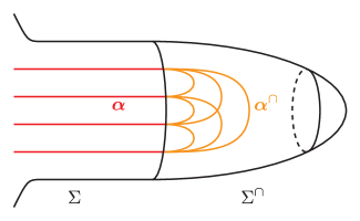
Figure 15. Capping off $\Sigma$. This figure is adapted from [LOT18, Figure 5.2].

First, we reduce to the case that all punctures are labeled by Reeb chords. Each boundary puncture labeled by a non-Reeby basic algebra element (of the form $U^{k}\iota_{j}$) increases the expected dimension by $1$, because it increases the dimension of $\mathfrak{M}$ by $1$ and otherwise does not affect the index, and also increases Formula (3.23) by $1$, because it increases $m$ by $1$. So, it suffices to consider the case that there are no punctures labeled $U^{k}\iota_{j}$. For punctures labeled $U^{k}\rho$, the integer $k$ does not affect the expected dimension or Formula (3.23). So, it suffices to assume all boundary punctures are labeled simply by Reeb chords.

Fix a curve $u\nobreak\mskip 2.0mu\mathpunct{}\nonscript\mkern-3.0mu{:}\penalty 300\mskip 6.0mu plus 1.0muS\to\Sigma\times[0,1]\times\mathbb{R}$ with the specified asymptotics. By (pre)gluing split curves to the boundary punctures, we can arrange that at each boundary puncture the curve $u$ is asymptotic to a Reeb chord of length $\leq 3$. Gluing each split curve increases both the expected dimension and $m$ by $1$, so it suffices to verify the result assuming each chord in $\vec{a}$ has length $\leq 3$. Similarly, one can replace a Reeb orbit with multiplicity $k>1$ with $k$ simple Reeb orbits by pregluing to the map $(z-1)\cdots(z-k)\nobreak\mskip 2.0mu\mathpunct{}\nonscript\mkern-3.0mu{:}\penalty 300\mskip 6.0mu plus 1.0mu\mathbb{C}\setminus\{1,\dots,k\}\to\mathbb{C}\setminus\{0\}$. This increases the expected dimension by $2(k-1)$, decreases $r$ in Formula (3.23) by $k-1$, and increases $w$ by $k-1$. So, we may assume $r=0$, that is, that every Reeb orbit is simple.

Now, glue the boundary of $\Sigma$ to a disk $\Sigma^{\cap}=\overline{\mathbb{H}}$ and glue the $\alpha$-arcs to the six arcs ${\boldsymbol{\alpha}}^{\cap}$ shown in Figure 15. Each of the Reeb chords in $u$ can be pre-glued to a holomorphic $1$-gon in $(\Sigma^{\cap},{\boldsymbol{\alpha}}^{\cap})$ and each Reeb orbit in $u$ can be pre-glued to a copy of $\Sigma^{\cap}$ itself to obtain a map $u^{\prime}\nobreak\mskip 2.0mu\mathpunct{}\nonscript\mkern-3.0mu{:}\penalty 300\mskip 6.0mu plus 1.0muS^{\prime}\to(\Sigma\cup\Sigma^{\cap})\times[0,1]\times\mathbb{R}$. From the closed case of the index formula [Lip06, Formula (6)], the expected dimension at $u^{\prime}$ is given by

$$\operatorname{ind}(u^{\prime})=g-\chi(S^{\prime})+2e(B^{\prime}).$$

We have $\chi(S^{\prime})=\chi(S)+w$ and $e(B^{\prime})=e(B)+m/2+w$. So,

$$\operatorname{ind}(u^{\prime})=g-\chi(S)-w+2e(B)+m+2w=g-\chi(S)+2e(B)+m+w.$$

On the other hand, each of the one-gons has index $1$ but the pre-gluing imposes a codimension-1 constraint, and each disk has index $2$ but gluing it to a Reeb orbit imposes a codimension-2 constraint. So, $\operatorname{ind}(u)=\operatorname{ind}(u^{\prime})$. This proves the result. ∎

Here is the analogue for boundary degenerations:

Proposition 3.24.

For a source $S^{\mspace{1.0mu}{\Box}}$ for a boundary degeneration, with the punctures other than $p_{\infty}$ labeled by a sequence of algebra elements $\vec{a}$, $w$ Reeb orbits with total ramification $r$, and covering $\Sigma$ with multiplicity $k$, and for any point $\mathbf{x}\in(\alpha_{1}^{a}\cup\alpha_{2}^{a}\cup\{p\})\times\alpha_{1}^{c}\times\cdots\times\alpha_{g-1}^{c}$, the expected dimension of the moduli space of holomorphic maps $\widetilde{\mathcal{N}}(\mathbf{x},S^{\mspace{1.0mu}{\Box}})$ is

(3.25) $$\operatorname{ind}(k,S^{\mspace{1.0mu}{\Box}},\vec{a};w,r)\coloneqq g-\chi(S)+2k(1-2g)+|\vec{a}|+\epsilon+w-r.$$

where $\epsilon=1$ if $p$ is a coordinate of $\mathbf{x}$ (i.e., the puncture $q_{\infty}$ is labeled by a Reeby element $U^{m}\rho$) and is $0$ otherwise.

(With regards to $\epsilon$, recall that the centered operations on $\mathcal{A}_{-}$ count simple boundary degenerations with index $2$.)

Proof.

We will assume that $p$ is not one of the coordinates of $\mathbf{x}$, though the other case is similar. As in the proof of Proposition 3.22, it suffices to assume that all of the punctures except $q_{\infty}$ are labeled simply by Reeb chords with $r=0$. We use a gluing argument, similar to the proof of Proposition 3.22. Fix a holomorphic curve $u\nobreak\mskip 2.0mu\mathpunct{}\nonscript\mkern-3.0mu{:}\penalty 300\mskip 6.0mu plus 1.0muS\to\Sigma\times\mathbb{H}$. Let $\overline{\mathbb{H}}$ denote the one-point compactification of $\mathbb{H}$. For each Reeb chord $\rho^{i}$ of $\Sigma$ preglue $u$ to one of the $1$-gons in Figure 15, as in the proof of Proposition 3.22, and for each Reeb orbit preglue $u$ to a $0$-gon. Here, the $1$-gons and $0$-gon are maps to $\Sigma^{\cap}\times\overline{\mathbb{H}}$ which map to $\overline{\mathbb{H}}$ by constant maps. In particular, the moduli space of $1$-gons has index $1$ and the moduli space of $0$-gons has index $2$, and pregluing imposes a $1$-dimensional (respectively $2$-dimensional) constraint for each $1$-gon (respectively $0$-gon). So, if we let $u^{\prime}\nobreak\mskip 2.0mu\mathpunct{}\nonscript\mkern-3.0mu{:}\penalty 300\mskip 6.0mu plus 1.0muS^{\prime}\to(\Sigma\cup\Sigma^{\cap})\times\overline{\mathbb{H}}$ denote the capped-off curve we have $\operatorname{ind}(u^{\prime})=\operatorname{ind}(u)+g+2r$: the $g$ comes from having replaced $\mathbb{H}$ by $\overline{\mathbb{H}}$ and, in the process, forgotten the codimension-$g$ constraint that $u$ passes through a specified point on each $\alpha$-curve at $\infty$. The index of the $\bar{\partial}$-operator at $u^{\prime}$ is given by $\operatorname{ind}(u^{\prime})=-\chi(S^{\prime})+2\mu$. These quantities satisfy

$$\chi(S^{\prime}) =\chi(S)+w$$

$$\mu =e(B)+|\vec{\rho}|/2+w+g+r.$$

(The $g$ comes from the Maslov index of the projection to $\overline{\mathbb{H}}$.) The Euler measure $e(B)$ is $k(1-2g)$. Combining these gives

$$\operatorname{ind}(u)=-\chi(S)-w+2e(B)+|\vec{\rho}|+2w+2g+r-g-2r=g-\chi(S)+2k(1-2g)+|\vec{\rho}|+w-r$$

as claimed. ∎

3.3.2. Embedded index formulas

Before stating the embedded index formulas we recall some notation.

Given a single Reeb chord $\rho$ starting at a point $s\in Z$ we define

(3.26) $$\iota(\rho)=-m(\boldsymbol{[}\rho\boldsymbol{]},s)$$

to be negative the average multiplicity of the support of $\rho$ near the point $s$. Explicitly, if $\rho$ has length $4k$ then $\iota(\rho)=-k$, while if $\rho$ has length $4k+\ell$, $1\leq\ell\leq 3$, then $\iota(\rho)=-k-1/2$. Given two chords $\rho,\rho^{\prime}$ we defined

(3.27) $$L(\rho,\rho^{\prime})=m(\boldsymbol{[}\rho^{\prime}\boldsymbol{]},\partial\boldsymbol{[}\rho\boldsymbol{]}),$$

the average multiplicity of the support of $\rho^{\prime}$ at the boundary of the support of $\rho$ [LOT18, Section 3.3.1]. For example, $L(\rho_{1},\rho_{2})=1/2=-L(\rho_{2},\rho_{1})$, $L(\rho_{1},\rho_{234})=0$, and $L(\rho_{1234}\rho^{\prime},\rho^{\prime\prime})=L(\rho^{\prime},\rho^{\prime\prime})$. In general, $L(\rho,\rho^{\prime})=-L(\rho^{\prime},\rho)$ (compare [LOT18, Lemma 3.35]).

Given a sequence $\vec{\rho}=(\rho^{1},\dots,\rho^{m})$ of Reeb chords, let

(3.28) $$\iota(\vec{\rho})=\sum_{i}\iota(\rho^{i})+\sum_{i<j}L(\rho^{i},\rho^{j})$$

(compare [LOT18, Formula (5.58)]).

Lemma 3.29.

If $\vec{\rho}=(\rho^{1},\dots,\rho^{m})$ is a sequence of Reeb chords so that the right idempotent of $\rho^{i}$ is equal to the left idempotent of $\rho^{i+1}$ for all $i$, then $\iota(\vec{\rho})$ is the Maslov component of

$$\operatorname{gr}^{\prime}(\rho^{1})\cdot\cdots\cdot\operatorname{gr}^{\prime}(\rho^{m}).$$

Proof.

Perform the product $\operatorname{gr}^{\prime}(\rho^{1})\cdot\cdots\cdot\operatorname{gr}^{\prime}(\rho^{m})$ so that it is right-associated (i.e., so that $\operatorname{gr}^{\prime}(\rho^{m-1})\operatorname{gr}^{\prime}(\rho^{m})$ is the first product, followed by $\operatorname{gr}^{\prime}(\rho^{m-2})(\operatorname{gr}^{\prime}(\rho^{m-1})\operatorname{gr}^{\prime}(\rho^{m}))$, and so on). The Maslov component of $\operatorname{gr}^{\prime}(\rho^{i})$ is, by definition, $\iota(\rho^{i})$. Let $\boldsymbol{[}\rho^{i}\boldsymbol{]}=(a,b,c,d)$ and $\boldsymbol{[}\rho^{i+1}\boldsymbol{]}+\cdots+\boldsymbol{[}\rho^{m}\boldsymbol{]}=(a^{\prime},b^{\prime},c^{\prime},d^{\prime})$. Then

$$\sum_{j\mid i<j}L(\rho^{i},\rho^{j}) =m\bigl{(}(a^{\prime},b^{\prime},c^{\prime},d^{\prime}),\partial(a,b,c,d)\bigr{)}$$

$$=\frac{1}{2}\bigl{(}(a-b)(a^{\prime}+b^{\prime})+(b-c)(b^{\prime}+c^{\prime})+(c-d)(c^{\prime}+d^{\prime})+(d-a)(d^{\prime}+a^{\prime})\bigr{)}$$

$$=\frac{1}{2}\left(\left|\begin{smallmatrix}a&b\\ a^{\prime}&b^{\prime}\end{smallmatrix}\right|+\left|\begin{smallmatrix}b&c\\ b^{\prime}&c^{\prime}\end{smallmatrix}\right|+\left|\begin{smallmatrix}c&d\\ c^{\prime}&d^{\prime}\end{smallmatrix}\right|+\left|\begin{smallmatrix}d&a\\ d^{\prime}&a^{\prime}\end{smallmatrix}\right|\right).$$

Comparing this to the formula for multiplication in $G^{\prime}$ gives the result. ∎

Next we state the embedded index formulas for holomorphic curves and boundary degenerations (the analogues of [LOT18, Proposition 5.62]), and a basic additivity property of these formulas. We turn to the proofs after we have given all the statements.

Recall that, given a domain $B$ and a tuple of points $\mathbf{x}$ in $\Sigma$, $n_{\mathbf{x}}(B)$ is the sum over the points $x_{i}$ in $\mathbf{x}$ of the average local multiplicity at $x_{i}$, and $e(B)$ is the Euler measure of $B$.

Proposition 3.30.

For an embedded holomorphic curve $u\nobreak\mskip 2.0mu\mathpunct{}\nonscript\mkern-3.0mu{:}\penalty 300\mskip 6.0mu plus 1.0muS\to\Sigma\times[0,1]\times\mathbb{R}$ in a homology class $B\in\pi_{2}(\mathbf{x},\mathbf{y})$ with sequence of basic algebra elements $\vec{a}$, underlying chord sequence $\vec{\rho}$, $w$ Reeb orbits, and total ramification $r$ at the Reeb orbits, we have

(3.31) $$\chi(S) =\chi_{{\mathrm{emb}}}(B,\vec{a},w,r)\coloneqq g+e(B)-n_{\mathbf{x}}(B)-n_{\mathbf{y}}(B)-\iota(\vec{\rho})+r$$

(3.32) $$\operatorname{ind}(u) =\operatorname{ind}(B,\vec{a},w,r)\coloneqq e(B)+n_{\mathbf{x}}(B)+n_{\mathbf{y}}(B)+|\vec{a}|+\iota(\vec{\rho})+w-2r.$$

Further, if $u$ has $d$ transverse double points (and is otherwise embedded) then $\chi(S)=\chi_{{\mathrm{emb}}}(B,\vec{\rho},w,r)+2d$ and $\operatorname{ind}(u)=\operatorname{ind}(B,\vec{\rho},w,r)-2d$.

That is, Formula (3.32) in the case $r=0$ gives the expected dimension of $\mathcal{M}^{B}(\mathbf{x},\mathbf{y};\vec{a};w)$. We will often write $\chi_{{\mathrm{emb}}}(B,\vec{a},w)$ and $\operatorname{ind}(B,\vec{a},w)$ for $\chi_{{\mathrm{emb}}}(B,\vec{a},w,0)$ and $\operatorname{ind}(B,\vec{a},w,0)$ (i.e., for curves where each Reeb orbit is simple).

Similar formulas to Proposition 3.30 compute the expected dimension of the space of embedded boundary degenerations. That is:

Proposition 3.33.

For a boundary degeneration as in Proposition 3.24, if the map to $\Sigma\times\mathbb{H}$ is an embedding and the projection to $\Sigma$ has degree $k$ then the Euler characteristic of $S^{\mspace{1.0mu}{\Box}}$ and the expected dimension of $\mathcal{N}(\mathbf{x};\vec{a};w,r)$ are given by

(3.34) $$\chi(S) =\chi_{{\mathrm{emb}}}(\vec{a},w,r)\coloneqq g+k(1-2g)-2kg-\iota(\vec{\rho})+r=g+k-4kg-\iota(\vec{\rho})+r$$

(3.35) $$\operatorname{ind}(u) =\operatorname{ind^{\square}}(\vec{a},w,r)\coloneqq k(1-2g)+2kg+|\vec{a}|+\epsilon+\iota(\vec{\rho})+w-2r$$

$$=k+|\vec{a}|+\epsilon+\iota(\vec{\rho})+w-2r$$

where $\vec{\rho}$ is the chord sequence underlying $\vec{a}$ and, as in Proposition 3.24, $\epsilon$ is $1$ if the asymptotic at $\infty$ is $U^{m}\rho$ and $0$ if the asymptotic at $\infty$ is $U^{m}\iota_{j}$.

Since we will most often be interested in the case $r=0$, let

$$\chi_{{\mathrm{emb}}}(\vec{a},w) =\chi_{{\mathrm{emb}}}(\vec{a},w,0) \operatorname{ind^{\square}}(\vec{a},w) =\operatorname{ind^{\square}}(\vec{a},w,0).$$

To know that the index formulas induce a well-behaved grading on the Floer complexes, we need to know they are additive:

Proposition 3.36.

Suppose $B\in\pi_{2}(\mathbf{w},\mathbf{x})$, $B^{\prime}\in\pi_{2}(\mathbf{x},\mathbf{y})$, $\vec{a}$ and $\vec{a}^{\prime}$ are sequences of Reeb chords compatible with $B$ and $B^{\prime}$, and $w$ and $w^{\prime}$ are non-negative integers. Let $(\vec{a},\vec{a}^{\prime})$ be the concatenation of the sequences $\vec{a}$ and $\vec{a}^{\prime}$. Then

$$\operatorname{ind}(B+B^{\prime},(\vec{a},\vec{a}^{\prime}),w+w^{\prime})=\operatorname{ind}(B,\vec{a},w)+\operatorname{ind}(B^{\prime},\vec{a}^{\prime},w^{\prime}).$$

To state the analogue for boundary degenerations, we need one more concept. Given a sequence of chords $\vec{\rho}$ and integers $w,r$, the domain multiplicity of $(\vec{\rho},w,r)$ is

(3.37) $$k=w+r+\frac{1}{4}\sum_{\rho^{i}\in\vec{\rho}}|\rho^{i}|.$$

Given a sequence of basic algebra elements $\vec{a}$, the domain multiplicity of $(\vec{a},w,r)$ is the domain multiplicity of $(\vec{\rho},w,r)$ where $\vec{\rho}$ is the underlying sequence of chords. If there is a boundary degeneration $u$ with Reeb chords $\vec{\rho}$, $w$ Reeb orbits and ramification $r$ at the Reeb orbits then the multiplicity of $u$ is $[\pi_{\Sigma}\circ u]=k[\Sigma]$, where $k$ is the domain multiplicity. In particular, the domain multiplicity is an integer. Additionally, the support $\boldsymbol{[}\vec{\rho}\boldsymbol{]}\in H_{1}(Z,\mathbf{a})$ of $\vec{\rho}$ is of the form $(\ell,\ell,\ell,\ell)$ (where $\ell=k-w-r$), that is, it is equal at $\rho_{1}$, $\rho_{2}$, $\rho_{3}$, and $\rho_{4}$. We call a sequence of chords $\vec{\rho}$ equidistributed if this latter condition holds, and call a sequence of basic algebra elements equidistributed if its underlying chord sequence is.

Lemma 3.38.

Let $B\in\pi_{2}(\mathbf{x},\mathbf{y})$, $\vec{a}=(a_{1},\dots,a_{n})$ and $\vec{a}^{\prime}=(a^{\prime}_{1},\dots,a^{\prime}_{m})$ be sequences of Reeb chords, and $w,w^{\prime},r,r^{\prime}\in\mathbb{Z}_{\geq 0}$. Assume that $\vec{a}^{\prime}$ is equidistributed and $k$ is the domain multiplicity of $(\vec{a}^{\prime},w^{\prime},r^{\prime})$. Fix $i$ and let

$$\vec{b}=(a_{1},\dots,a_{i},a^{\prime}_{1},\dots,a^{\prime}_{m},a_{i+1},\dots,a_{n})$$

Then

$$\operatorname{ind}(B+k[\Sigma],\vec{b},w+w^{\prime},r+r^{\prime})=\operatorname{ind}(B,\vec{a},w,r)+\operatorname{ind^{\square}}(\vec{a}^{\prime},w^{\prime},r^{\prime}).$$

(This corresponds to the case of a simple boundary degeneration.)

Similarly, if we let

$$\vec{b}^{\prime}=(a_{1},\dots,a_{i}a^{\prime}_{1},a^{\prime}_{2},\dots,a^{\prime}_{m},a_{i+1},\dots,a_{n})$$

or

$$\vec{b}^{\prime}=(a_{1},\dots,a_{i},a^{\prime}_{1},\dots,a^{\prime}_{m-1},a^{\prime}_{m}a_{i+1},\dots,a_{n})$$

then

$$\operatorname{ind}(B+k[\Sigma],\vec{b}^{\prime},w+w^{\prime},r+r^{\prime})=\operatorname{ind}(B,\vec{a},w,r)+\operatorname{ind^{\square}}(\vec{a}^{\prime},w^{\prime},r^{\prime})-1.$$

(This corresponds to the case of a composite boundary degeneration.)

The proofs of the embedded index formulas will be based on Sarkar’s index formula for polygons [Sar11], so we recall that next. Fix a (classical, not bordered) Heegaard multi-diagram $(\Sigma_{g},{\boldsymbol{\alpha}}^{1},\dots,{\boldsymbol{\alpha}}^{n})$, points $\mathbf{x}^{i,i+1}\in T_{{\boldsymbol{\alpha}}^{i}}\cap T_{{\boldsymbol{\alpha}}^{i+1}}\subset\operatorname{Sym}^{g}(\Sigma)$, and a point $\mathbf{x}^{n,1}\in T_{{\boldsymbol{\alpha}}^{n}}\cap T_{{\boldsymbol{\alpha}}^{1}}$. Assume that ${\boldsymbol{\alpha}}^{i}\pitchfork{\boldsymbol{\alpha}}^{j}$ for $i\neq j$. Given oriented arcs $A\subset{\boldsymbol{\alpha}}^{i}$ and $B\subset{\boldsymbol{\alpha}}^{j}$, $i\neq j$, define the jittered intersection number $A\cdot B$ of $A$ and $B$ as follows. If $A$ and $B$ intersect only at interior points then $A\cdot B$ is their intersection number in the usual sense. Otherwise, if, say, an endpoint of $A$ intersects $B$ then there are four directions one can push $A$ off ${\boldsymbol{\alpha}}^{i}$ slightly so that the pushoff is transverse to ${\boldsymbol{\alpha}}^{j}$ (and hence $B$); let $A\cdot B$ be the average of the four intersection numbers of these pushoffs with $B$. So, $A\cdot B\in\frac{1}{4}\mathbb{Z}$.

Given a homotopy class of $n$-gons $D\in\pi_{2}(\mathbf{x}^{1,2},\mathbf{x}^{2,3},\dots,\mathbf{x}^{n,1})$, Sarkar proves that the Maslov index of $D$ (expected dimension of the moduli space with a fixed complex structure on the source) is

(3.39) $$\mu(D)=e(D)+n_{\mathbf{x}^{1,2}}(D)+n_{\mathbf{x}^{n,1}}(D)-\left(\sum_{1<i<j\leq n}\partial^{{\boldsymbol{\alpha}}^{i}}(D)\cdot\partial^{{\boldsymbol{\alpha}}^{j}}(D)\right)-\frac{g(n-2)}{2}.$$

Here, $\partial^{{\boldsymbol{\alpha}}^{i}}(D)$ is the part of the cellular $1$-chain $\partial D$ lying in ${\boldsymbol{\alpha}}^{i}$ and $\cdot$ denotes the jittered intersection number. The $n$-gon maps on Heegaard Floer homology count holomorphic $n$-gons with Maslov index $3-n$. In the case of a bigon in $\pi_{2}(\mathbf{x},\mathbf{y})$, Formula (3.39) reduces to the familiar formula $e(D)+n_{\mathbf{x}}(D)+n_{\mathbf{y}}(D)$.

Proof of Propositions 3.30 and 3.33.

We will prove the formulas for the index at embedded holomorphic curves; the formulas for the Euler characteristic of the source then follow from Propositions 3.22 and 3.24.

It suffices to prove the result when $\vec{a}$ consists entirely of chords. Specifically, the proof we will give does not depend on the particular choice of almost complex structure. The $U$-powers labeling punctures only affect the choice of almost complex structure, as do punctures labeled $U^{n}\iota_{j}$ (except for adding $1$ to both the expected dimension and Formula (3.32)).

By additivity of the index under gluing, if $\rho^{i}=\rho^{\prime}\rho^{\prime\prime}$ then the expected dimension of the moduli space of curves asymptotic to $(\rho^{1},\dots,\rho^{i},\dots,\rho^{n})$ is one less than the expected dimension of the moduli space of curves asymptotic to $(\rho^{1},\dots,\rho^{\prime},\rho^{\prime\prime},\dots,\rho^{n})$: the two differ by gluing on a split curve. Replacing $(\rho^{1},\dots,\rho^{i},\dots,\rho^{n})$ by $(\rho^{1},\dots,\rho^{\prime},\rho^{\prime\prime},\dots,\rho^{n})$ also increases the right side of Equation (3.32): the only term that changes is $|\vec{\rho}|$. (The fact that $\iota$ does not change follows from Lemma 3.29.) So, it suffices to prove the result when all of the chords $\rho^{i}$ have length $1$. Similarly, we can assume that all of the Reeb orbits are simple.

After these simplifications, the index $\operatorname{ind}$ is essentially the same as the Maslov index in the symmetric product, under the tautological correspondence (Section 3.2.5). More precisely, because $\mu$ gives the expected dimension for polygons with a fixed conformal structure and $\operatorname{ind}$ allows the conformal structure to vary,

$$\operatorname{ind}(u)=\mu(B)+|\vec{\rho}|.$$

The next step is to apply Sarkar’s formula to compute $\mu(B)$. For definiteness, assume that a point of $\mathbf{x}$ lies on $\alpha_{1}^{a}$. Then (since all the $\rho^{i}$ have length $1$, which is odd), the polygon has boundary

$$(T_{\boldsymbol{\beta}},T_{{\boldsymbol{\alpha}},1},T_{{\boldsymbol{\alpha}},2},T_{{\boldsymbol{\alpha}},1},\dots,T_{{\boldsymbol{\alpha}},(1+|\vec{\rho}|)\bmod 2}).$$

In particular, the same $\alpha$-curves are repeated many times. To apply Sarkar’s formula, we must first choose perturbations of these $\alpha$-curves to make them transverse. How we do this perturbation affects $n_{\mathbf{x}}$, $n_{\mathbf{y}}$, and the $\partial^{{\boldsymbol{\alpha}}^{i}}(D)\cdot\partial^{{\boldsymbol{\alpha}}^{j}}(D)$ terms.

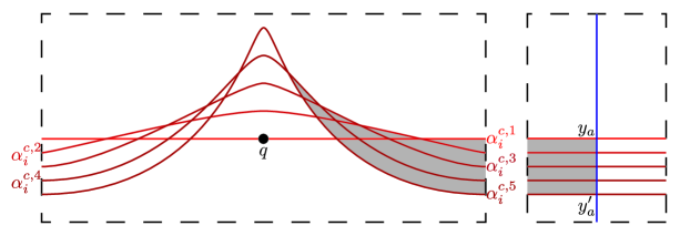
Figure 16. Perturbing $\alpha$-circles. The figure corresponds to the case $|\vec{\rho}|=4$. The original intersection point $y_{a}\in\alpha_{a}^{c}\cap\beta_{b}$, the corresponding point $y^{\prime}_{a}\in\alpha_{a}^{c,5}\cap\beta_{b}$, and the point $q$ are also indicated.

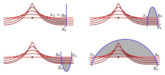
Figure 17. Multiplicities in the perturbed diagram. In the first case, $n_{\mathbf{x}}$ and $n_{\mathbf{y}}$ both increase by $1/4$. In the second, $n_{\mathbf{x}}$ increases by $1/2$ while $n_{\mathbf{y}}$ is unchanged. In the third, $n_{\mathbf{x}}$ is unchanged while $n_{\mathbf{y}}$ increases by $1/2$. In the fourth, $n_{\mathbf{x}}$ and $n_{\mathbf{y}}$ are both unchanged. In the first three cases, $\ell=0$ and the jittered intersection number is $-(4-2)/4+0=-1/2$, while in the last $\ell=1$ and the jittered intersection number is $-(4-2)/2+1/2=0$.

For each $\alpha$-circle $\alpha_{m}^{c}$, choose the perturbations $\alpha_{m}^{c,i}$ as shown in Figure 16, so that $\alpha_{m}^{c,i}$ and $\alpha_{m}^{c,j}$ are disjoint outside the figure for $i\neq j$ and the points $\mathbf{x}$ and $\mathbf{y}$ are outside the region where the perturbed circles intersect each other. Locally, the perturbed domain is obtained from the original domain of bigons by gluing on (adding) the shaded region in the figure. The Euler measure of the shaded region is $|\vec{\rho}|/4$ and the jittered intersection number is $-(|\vec{\rho}|-2)/4+\ell/2$, where $\ell$ is the multiplicity with which a point $q$ on $\alpha_{m}^{c}$ in the perturbation region occurs in $\partial^{\alpha}B$. The perturbation increases $n_{\mathbf{x}}+n_{\mathbf{y}}$ by $1/2-\ell/2$. (See Figure 17 for some examples.) So, the contribution to Formula (3.39) is $|\vec{\rho}|/2-1/2+\ell/2-\ell/2+1/2=|\vec{\rho}|/2$. There are $g-1$ such $\alpha$-circles, for a total contribution of

$$\frac{(g-1)|\vec{\rho}|}{2}.$$

We claim that for the $\alpha$-arcs we can apply Sarkar’s formula without perturbing. We prove this by induction on the number of $\alpha$-arcs not perturbed. Suppose the formula holds if the first $\ell$ copies of the $\alpha_{i}^{a}$ are not perturbed. There are two natural directions to push off the $(\ell+1)^{\text{st}}$ copy of an $\alpha$-arc. The Euler measure of the domain is the same whether the $\alpha$-arc is perturbed or not. By definition, the $n_{\mathbf{x}^{1,2}}$ and $n_{\mathbf{x}^{n,1}}$ terms and the $\partial^{{\boldsymbol{\alpha}}^{i}}\cdot\partial^{{\boldsymbol{\alpha}}^{j}}$-terms for the un-perturbed curve are the average of the terms for the two directions of perturbing (since both can be viewed as averages over pushing off the $\alpha$-curve in four directions). So, since the formula holds for either direction of perturbation, it also holds for the average of the two directions, i.e., for not perturbing at all.

For the un-perturbed $\alpha$-arcs, the big sum in Formula (3.39) contributes

$$-\frac{1}{4}|\vec{\rho}|+\sum_{i<j}L(\rho^{i},\rho^{j})=\frac{1}{2}\sum_{i}\iota(\rho^{i})+\sum_{i<j}L(\rho^{i},\rho^{j});$$

see Figure 18.

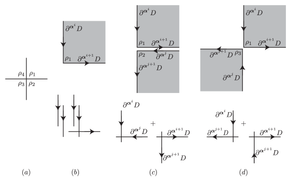
Figure 18. Jittered intersection numbers and chords. (a) The chords around the point $p=\alpha_{1}^{a}\cap\alpha_{2}^{a}$. (b) The contribution to the jittered intersection number $\partial^{{\boldsymbol{\alpha}}^{i}}D\cdot\partial^{{\boldsymbol{\alpha}}^{i+1}}D$ coming from the arcs into and out of $\rho_{1}$ is $1/4$. (c) The contribution from a chord $\rho_{1}$ followed later by a chord $\rho_{2}$ is $-1/2$, while the contribution from $\rho_{2}$ followed later by $\rho_{1}$ is $+1/2$. (d) The contribution from $\rho_{1}$ followed later by $\rho_{3}$ is $0$, since in this case the two nonzero terms cancel. The other combinations of length-1 chords are similar.

Finally, for Formula (3.39), each Reeb chord corresponds to a $\pi/2$-corner, so contributes $-1/4$ to the Euler measure. For Formula (3.32), each Reeb chord is viewed as having two $\pi/2$-corners, so contributes $-1/2$ to the Euler measure. Also, each orbit contributes $0$ to Formula (3.39) but $-1$ to Formula (3.32). So, the Euler measure term in Formula (3.39) is actually

$$e(B)+\frac{1}{4}|\vec{\rho}|+w.$$

Adding up these contributions, Formula (3.39) gives

$$\operatorname{ind}(B,\vec{\rho},w,0) =e(B)+\frac{1}{4}|\vec{\rho}|+w+n_{\mathbf{x}}(B)+n_{\mathbf{y}}(B)-\frac{1}{4}|\vec{\rho}|+\sum_{i<j}L(\rho^{i},\rho^{j})$$

$$\qquad\qquad\qquad\qquad+\frac{(g-1)|\vec{\rho}|}{2}-\frac{g|\vec{\rho}|}{2}+|\vec{\rho}|$$

$$=e(B)+w+n_{\mathbf{x}}(B)+n_{\mathbf{y}}(B)+\sum_{i<j}L(\rho^{i},\rho^{j})+\frac{|\rho|}{2}$$

$$=e(B)+2+n_{\mathbf{x}}(B)+n_{\mathbf{y}}(B)+|\vec{\rho}|+\sum_{i}\iota(\rho^{i})+\sum_{i<j}L(\rho^{i},\rho^{j})$$

$$=e(B)+n_{\mathbf{x}}(B)+n_{\mathbf{y}}(B)+|\vec{\rho}|+\iota(\vec{\rho})+w,$$

as desired. ∎

Proof of Proposition 3.36 and Lemma 3.38.

This is immediate from the fact that these index formulas agree with the Maslov index in the symmetric product and additivity of the Maslov index. ∎

Remark 3.40.

In the case of $\widehat{\mathit{HF}}$, instead of reducing to Sarkar’s formula we proved the embedded index formula (the analogue of Proposition 3.30) by studying how a holomorphic curve intersects its translates (similar to the computation in the closed case [Lip06]). That argument requires the almost complex structure be a product near the boundary of the strip, to avoid having intersection points disappear on the boundary, so does not apply immediately to the kinds of almost complex structures considered here. On the other hand, the argument relying on Sarkar’s formula would not apply directly to the higher genus boundary case of bordered Floer theory, since there is not a direct identification with Heegaard multi-diagrams in that case.

3.4. Pinched almost complex structures

So far, we have not explained the role of the pinching function (Definition 3.2). In this section, we will see one reason it is required. (The other is in Section 4.)

Lemma 3.41.

Given a sequence of basic algebra elements $\vec{a}$ and non-negative integers $w$ and $r$, for any $\epsilon$ sufficiently small (depending on $\vec{a}$, $w$, and the bordered Heegaard diagram), if $j$ is an $\epsilon$-pinched complex structure for which $\mathcal{N}(\mathbf{x},\vec{a};w,r)$ contains a non-constant curve, then

$$\operatorname{ind^{\square}}(\vec{a},w,r)\geq 2.$$

Further, if $\operatorname{ind^{\square}}(\vec{a},w,r)=2$ then no pair of consecutive elements of $\vec{a}$ are multipliable, i.e., have $a_{i}a_{i+1}\neq 0$. In particular, no element of $\vec{a}$ has the form $U^{n}\iota_{j}$.

Proof.

We start by reducing to the genus $1$ case, using the $\epsilon$-pinched condition. Fix a sequence $\epsilon_{i}\to 0$ and suppose the moduli spaces $\mathcal{N}(\mathbf{x};\vec{a};w,r)$ are non-empty with respect to a sequence of $\epsilon_{i}$-pinched almost complex structures. Choose a convergent subsequence of these complex structures. In the limit, we obtain a complex structure on the genus-1 surface containing $\alpha_{1}^{a}\cup\alpha_{2}^{a}$ so that the compactified moduli space $\overline{\mathcal{N}}{}(\mathbf{x};\vec{a};w,r)$ is non-empty for this complex structure. This moduli space consists of trees of holomorphic disks mapped to a genus-1 surface (because the map to $\mathbb{H}$ is a 1-fold branched cover); such holomorphic maps are determined by their combinatorics and branched points. In particular, it is easy to see that, in the genus $1$ case, whenever the compactified moduli space $\overline{\mathcal{N}}{}(\mathbf{x};\vec{a};w,r)$ is non-empty, the uncompactified space $\mathcal{N}(\mathbf{x};\vec{a};w,r)$ is also non-empty.

So, it suffices to prove the result in the case that $g=1$. Fix a boundary degeneration $u\nobreak\mskip 2.0mu\mathpunct{}\nonscript\mkern-3.0mu{:}\penalty 300\mskip 6.0mu plus 1.0muS\to\Sigma\times\mathbb{H}$. As observed above, since $\pi_{\mathbb{H}}\circ u$ is a 1-fold branched cover of $\mathbb{H}$, $S$ has genus $0$. So, $\chi(S)=1-w+r$. On the other hand, $\pi_{\Sigma}\circ u$ is a branched cover of degree $k>0$. So, if $\operatorname{br}$ denotes the ramification number of $\pi_{\Sigma}\circ u$ and the homology class of $\pi_{\Sigma}\circ u$ is $k[\Sigma]$ then by the Riemann-Hurwitz formula, $\chi(S)=-k+|\vec{\rho}|/2-\operatorname{br}$, where $\rho$ is the associated chord sequence. (Specifically, the Euler measures satisfy $e(S)=ke(\Sigma)-\operatorname{br}=-k-\operatorname{br}$ and the Euler characteristic of $S$ is $\chi(S)=e(S)+|\vec{\rho}|/2$: since when computing $e$ each puncture corresponds to an arc with two corners at its end, each puncture decreases $e(S)$ by $2/4$.) So,

$$w+|\vec{\rho}|/2-r=1+k+\operatorname{br}.$$

Hence, by Proposition 3.24, the index is given by

$$\operatorname{ind^{\square}}(\vec{a},w,r)\geq\operatorname{ind^{\square}}(\vec{\rho},w,r)=1-1+w-r-2k+|\vec{\rho}|+w-r=-2k+|\vec{\rho}|+2w-2r=2+2\operatorname{br}.$$

Thus, the index is at least $2$. Further, if the index is equal to $2$ then the first inequality is an equality so $|\vec{a}|=|\vec{\rho}|$, hence no element of $\vec{a}$ has the form $U^{n}\iota_{j}$. Finally, to see that no pair of consecutive chords in $\vec{\rho}$ are multipliable, note that if $\rho^{i}$ and $\rho^{i+1}$ are multipliable then there is a boundary branch point of $\pi_{\Sigma}\circ u$ between the corresponding punctures, so $\operatorname{br}\geq 1/2$ and hence the index is at least $3$. ∎

Since for any $C$ there are finitely many pairs of a sequence of basic algebra elements $\vec{a}$ and non-negative integer $w$ so that the energy satisfies $E(\vec{a},w)\leq C$, by Lemma 3.41, for each energy $C$ there is an $\eta(C)>0$ so that if $J$ is $\eta(C)$-pinched then the conclusion of Lemma 3.41 hold for any $(\vec{a},w,r)$ with energy $E(\vec{a},w)\leq C$. This is the condition we require for our pinching function:

Definition 3.42.

A pinching function $\eta$ is sufficient if for each positive integer $C$, for every $(\vec{a},w)$ with $E(\vec{a},w)\leq C$, Lemma 3.41 holds for $(\vec{a},w)$ with $\epsilon=\eta(C)$.

Corollary 3.43.

There exist sufficient pinching functions.

Proof.

This is immediate from Lemma 3.41. ∎

3.5. Transversality

We recall two results of Ozsváth-Szabó about the non-existence of sphere and disk bubbles. For both spheres in $\operatorname{Sym}^{g}(\Sigma)$ and disks in $\operatorname{Sym}^{g}(\Sigma)$ with boundary on some $T_{\alpha,i}$ or $T_{\beta}$, the homology class is a multiple of $\Sigma$. Positivity of domains implies that the moduli spaces in homology class $n[\Sigma]$ are empty unless $n>0$. The relevance of this to the moduli spaces under consideration is via the tautological correspondence from Section 3.2.5.

Lemma 3.44.

[OSz04, Lemma 3.13] Given any complex structure $i$ on $\Sigma$, the set of points in $\operatorname{Sym}^{g}(\Sigma)$ lying on holomorphic spheres has codimension $2$.

Corollary 3.45.

For a generic choice of complex structure $i$ on $\Sigma$ and any $\mathbb{R}$-invariant admissible almost complex structure $J$ sufficiently close to $i\times j_{\mathbb{D}}$, there are no holomorphic spheres through points in $(T_{\alpha,1}\cup T_{\alpha,2})\cap T_{\beta}$.

Proof.

This is immediate from the previous lemma and Gromov compactness. ∎

Lemma 3.46.

[OSz04, Theorem 3.15] If the moduli space of disks with boundary on $T_{\beta}$ (respectively $T_{\alpha,1}$, $T_{\alpha,2}$) through a given point $p\in T_{\beta}$ (respectively $p\in T_{\alpha,1}$, $p\in T_{\alpha,2}$) is transversely cut out, then the count of Maslov index $2$ disks through $p$ vanishes.

Next, we turn to the transversality we will need for boundary degenerations, continuing with the discussion from Section 3.2.4:

Definition 3.47.

The complex structure $j$ is called regular for energy $E_{0}$ boundary degenerations if for all $(\vec{a};w,r)$ with $\operatorname{ind^{\square}}(\vec{a};w,r)\leq 2$ and $E(\vec{a},w)\leq E_{0}$, the moduli space $\mathcal{N}(*;\vec{a};w,r)$ is smoothly cut out, and every generator $\mathbf{x}$ is a regular value of the evaluation map $\operatorname{ev}\nobreak\mskip 2.0mu\mathpunct{}\nonscript\mkern-3.0mu{:}\penalty 300\mskip 6.0mu plus 1.0mu\mathcal{N}(*;\vec{a};w,r)\to(\alpha_{1}^{a}\cup\alpha_{2}^{a})\times\alpha^{c}_{1}\times\dots\times\alpha^{c}_{g-1}$.

In particular, if $j$ is regular for energy $E_{0}$ boundary degenerations then for generic $\mathbf{x}$ and $E(\vec{a},w)\leq E_{0}$, the space $\mathcal{N}(\mathbf{x};\vec{a};w)$ is a smooth manifold of dimension $\operatorname{ind^{\square}}(\vec{a};w)-2$.

The proof of existence of regular $j$ is given in Theorem 4.3 below.

Next we discuss the dependence of the moduli space of boundary degenerations based at $\mathbf{x}$ on the point $\mathbf{x}$:

Lemma 3.48.

Suppose that $\operatorname{ind^{\square}}(\vec{a},w,r)=2$ and $j$ is regular for energy $E(\vec{a},w)$ boundary degenerations and is $\eta(E(\vec{a},w))$-pinched for some sufficient pinching function $\eta$. Then, the map

$$\operatorname{ev}\nobreak\mskip 2.0mu\mathpunct{}\nonscript\mkern-3.0mu{:}\penalty 300\mskip 6.0mu plus 1.0mu\mathcal{N}(*;\vec{a};w,r)\to(\alpha_{1}^{a}\cup\alpha_{2}^{a})\times\alpha^{c}_{1}\times\dots\times\alpha^{c}_{g-1}$$

is proper.

Proof.

The proof is similar to, but easier than, the proof of Theorem 1.12 in Section 3.7, but we will also give fewer details than in that proof, so the reader may find it easier to read that proof first.

Fix a sequence in $\mathcal{N}(*;\vec{a};w,r)$. Considering just the images in $\mathbb{H}$ of the punctures gives a sequence of algebra-type polygons. By compactness of $\mathfrak{M}$, by taking a subsequence we may assume this sequence of polygons converges in $\mathfrak{M}$, to some tree of disks (perhaps union some sphere bubbles). Then, applying Gromov compactness (or the version from symplectic field theory [BEH⁺03], if we think of the marked points of the disks as punctures), we may assume that the sequence of holomorphic curves itself converges. The limit is either an element of $\mathcal{N}(*;\vec{a};w,r)$ or a broken polygon (perhaps union some sphere bubbles). In the former case, the result is immediate from continuity of the evaluation map, so it remains to rule out the latter case. It follows from the second half of Lemma 3.41 (the statement about no consecutive pair of chords being multipliable) that any constant component mapped to $p$ (i.e., curve at $e\infty$) connects to at least two other components. So, there are at least two non-constant components. But this violates Lemma 3.41 and additivity of the index (Lemma 3.38). ∎

Lemmas 3.41 and 3.48 imply that the spaces $\mathcal{N}(\mathbf{x},\vec{a};w,r)$ for different regular values $\mathbf{x}$ of $\operatorname{ev}$ (intersecting the same $\alpha$-arc) are cobordant. So, we will often want to fix $\mathbf{x}$ but not include it in the notation. Let

$$\mathcal{N}([\alpha_{i}^{a}];\vec{a};w) =\mathcal{N}(\mathbf{x};\vec{a};w),$$

where $\alpha_{i}^{a}$ is the $\alpha$-arc containing a coordinate in $\mathbf{x}$. By Lemma 3.41, if $\operatorname{ind^{\square}}(\vec{a},w)=2$ and $\mathcal{N}([\alpha_{i}^{a}];\vec{a};w)\neq\emptyset$ then all of the $a_{i}$ are Reeby elements. Also, if $a_{1}=U^{\ell}\rho^{1}$ and $a_{n}=U^{m}\rho^{n}$, then necessarily $\alpha_{i}^{a}=[(\rho^{1})^{-}]=[(\rho^{n})^{+}]$, the $\alpha$-arc containing the initial endpoint of $\rho^{1}$ and the terminal endpoint of $\rho^{n}$.

Definition 3.49.

For $i=1,2$, let $\#\mathcal{N}([\alpha_{i}^{a}];\vec{a};w)$ be the number of points in $\mathcal{N}(\mathbf{x};\vec{a};w))$, for a generic choice of point $\mathbf{x}$ with a component in $\alpha_{i}^{a}$. (It follows from Lemma 3.48 that this number is independent of the choice of $\mathbf{x}$.)

In Section 4, we prove that the degrees appearing in Definition 3.49 are independent of the choice of $j$; indeed, according to Theorem 1.5 (also proved in that section), these are identified with terms in the operations on $\mathcal{A}_{-}$.

Returning to the main component, we have:

Proposition 3.50.

For any pinching function $\eta$, the set of coherent families of $\eta$-admissible almost complex structures so that the moduli spaces $\mathcal{M}^{B}(\mathbf{x},\mathbf{y};{S^{\mspace{1.0mu}\triangleright}})$ are all transversely cut out is co-meager. Similarly, the set of coherent families of $\eta$-admissible almost complex structures so that the moduli spaces of disks appearing in Lemma 3.46 are transversely cut out is also co-meager.

Proof.

This is an easy adaptation of the case for bordered $\widehat{\mathit{HF}}$ [LOT18], which in turn is an adaptation of the cylindrical case for Heegaard Floer homology [Lip06, Section 3] (which in turn is adapted from McDuff-Salamon [MS04]). (For the second statement in the proposition note that the domain of a Maslov index $2$ disk is a copy of $\Sigma$, so these disks are somewhere injective—in fact, injective at every interior point.) ∎

Finally, we collect all of the transversality conditions we will require for the modules $\mathit{CFA}^{-}$ and $\mathit{CFD}^{-}$ to be defined:

Definition 3.51.

Call an $\eta$-admissible family of almost complex structures $J$ tailored if the following conditions hold:

1. The pinching function $\eta$ is sufficient in the sense of Definition 3.42.

2. The moduli spaces $\mathcal{M}^{B}(\mathbf{x},\mathbf{y};{S^{\mspace{1.0mu}\triangleright}})$ are transversely cut out for all data $(B,{S^{\mspace{1.0mu}\triangleright}},\vec{a},w,r)$ such that $\operatorname{ind}(B,{S^{\mspace{1.0mu}\triangleright}},\vec{a},w,r)\leq 2$.

3. For each sequence of basic algebra elements $\vec{a}$, integer $w$, decorated source ${S^{\mspace{1.0mu}\triangleright}}$ compatible with $(\vec{a},w)$, and homology class $B$ so that $\operatorname{ind}(B,{S^{\mspace{1.0mu}\triangleright}},\vec{a};w,r)\leq 1$ and each $a_{i}\in\vec{a}$, the following holds. Let $q_{i}$ be the puncture of ${S^{\mspace{1.0mu}\triangleright}}$ corresponding to $a_{i}$.

   • If $a_{i}=U^{n}\iota_{j}$ then for each $u\in\mathcal{M}^{B}(\mathbf{x},\mathbf{y};{S^{\mspace{1.0mu}\triangleright}})$, the complex structure on $\Sigma$ corresponding to $q_{i}$ is regular for energy $E(a_{i})$ boundary degenerations, and $\mathbf{w}=\pi_{\Sigma}(u(q_{i}))$ is a regular value of each evaluation map $\operatorname{ev}\nobreak\mskip 2.0mu\mathpunct{}\nonscript\mkern-3.0mu{:}\penalty 300\mskip 6.0mu plus 1.0mu\mathcal{N}(*;\vec{a}^{\prime};w^{\prime},r^{\prime})\to(\alpha_{1}^{a}\cup\alpha_{2}^{a})\times\alpha_{1}^{c}\times\cdots\times\alpha_{g-1}^{c}$, for each sequence of basic algebra elements $a^{\prime}$ and integers $w^{\prime}$ and $r^{\prime}$ so that the moduli space has index $\leq 2$. So, the index $\leq 2$ moduli spaces $\mathcal{N}(\mathbf{w};S^{\mspace{1.0mu}{\Box}})$ are transversely cut out.

   • If $a_{i}=U^{n}\rho$ then for each $u\in\mathcal{M}^{B}(\mathbf{x},\mathbf{y};{S^{\mspace{1.0mu}\triangleright}})$, the complex structure on $\Sigma$ corresponding to $q_{i}$ is regular for energy $E(a_{i})$ boundary degenerations, and if we let $p\times\mathbf{w}=\pi_{\Sigma}(u(q_{i}))$, where $\mathbf{w}\in\alpha_{1}^{c}\times\cdots\times\alpha_{g-1}^{c}$, then the moduli spaces $\mathcal{N}(\rho^{i}\times\mathbf{w};S^{\mspace{1.0mu}{\Box}})$ with index $\leq 2$ are transversely cut out.

   (By Condition (TJ-2), there are finitely many holomorphic curves $u$ for each tuple of data $(\vec{a},w,{S^{\mspace{1.0mu}\triangleright}},B)$, so this amounts to countably many conditions overall. Also, the moduli spaces $\mathcal{N}$ here are computed with respect to the complex structure induced by $J$ at $q_{i}$.)

4. There is no $\operatorname{Sym}^{g}(j)$-holomorphic sphere in $\operatorname{Sym}^{g}(\Sigma)$ passing through any point in $(T_{\alpha,1}\cup T_{\alpha,2})\cap T_{\beta}$, for any complex structure $j$ appearing in $J_{\infty}$.

5. The moduli spaces of $J_{\infty}$-holomorphic disks with boundary on $T_{\beta}$ and index $\leq 2$ are transversely cut out, as are the moduli spaces of holomorphic disks with boundary on $T_{\alpha,1}$ and the moduli space of disks with boundary on $T_{\alpha,2}$.

Corollary 3.52.

Tailored families almost complex structures exist.

Proof.

Fix a sufficient pinching function (Condition (TJ-1)), which exists by Corollary 3.43. Conditions (TJ-4), (TJ-5), and the special case of (TJ-2) with no algebra punctures give restrictions on the $\mathbb{R}$-invariant almost complex structure $J_{\infty}$ from Condition (1). By Corollary 3.45 and Proposition 3.50, a generic almost complex structure close to a split one satisfies these conditions. So, start by fixing such a generic, $\mathbb{R}$-invariant almost complex structure $J_{\infty}$. Then, construct the admissible family of almost complex structures as in the proof of Lemma 3.7, agreeing with $J_{\infty}$ near $\pm\infty$, using Proposition 3.50 to guarantee the moduli spaces $\mathcal{M}$ are transversely cut out (Condition (TJ-2)). To ensure Condition (TJ-3), by Sard’s theorem, for generic points $\mathbf{w}\in\alpha_{1}^{c}\times\cdots\times\alpha_{g-1}^{c}$ and $\mathbf{w}^{\prime}\in(\alpha_{1}^{a}\cup\alpha_{2}^{a})\times\alpha_{1}^{c}\times\cdots\times\alpha_{g-1}^{c}$, the moduli spaces $\mathcal{N}(\rho\times\mathbf{w};S^{\mspace{1.0mu}{\Box}})$ and $\mathcal{N}(\mathbf{w}^{\prime};S^{\mspace{1.0mu}{\Box}})$ are smoothly cut out. For a generic choice of $J$, the moduli spaces $u\in\mathcal{M}^{B}(\mathbf{x},\mathbf{y};{S^{\mspace{1.0mu}\triangleright}})$ with $\operatorname{ind}(B,{S^{\mspace{1.0mu}\triangleright}},\vec{a};w,r)=1$ will only be asymptotic to such generic $(\rho,\mathbf{w})$, giving Condition (TJ-3). ∎

3.6. Gluing

In this section, we prove gluing theorems corresponding to the different cases in Theorem 1.12. In each case, to state the gluing theorem we need to define what it means for a family of unbroken holomorphic curves (as in Section 3.2.2) to converge to a broken holomorphic curve, since the gluing theorems assert that near a broken curve, the space of unbroken curves has a particular form (or, more precisely, a single end).

A two-story building is a pair

$$(u,u^{\prime})\in\mathcal{M}^{B}(\mathbf{x},\mathbf{x}^{\prime};a_{1},\dots,a_{j};w_{1})\times\mathcal{M}^{B^{\prime}}(\mathbf{x}^{\prime},\mathbf{y};a_{j+1},\dots,a_{n};w_{2}).$$

Convergence to a two-story building is the usual notion from symplectic field theory [BEH⁺03]: a sequence of holomorphic curves $u_{i}\in\mathcal{M}^{B_{1}+B_{2}}(\mathbf{x},\mathbf{y};a_{1},\dots,a_{n};w_{1}+w_{2})$ as in Definition 3.14 converges to a two-story building $(u^{1},u^{2})$ if, as in [LOT18, Definition 5.21], the maps $\pi_{\Sigma}\circ u_{i}$ and $\pi_{\mathbb{D}}\circ u_{i}$ converge to $(\pi_{\Sigma}\circ u^{1},\pi_{\Sigma}\circ u^{2})$ and $(\pi_{\mathbb{D}}\circ u^{1},\pi_{\mathbb{D}}\circ u^{2})$ in the sense of [BEH⁺03]. (Implicitly, we also are assuming that the polygons $P_{i}\in\mathfrak{M}$ underlying the $u_{i}$ converge to the broken polygon $(P,P^{\prime})$ corresponding to $(u,u^{\prime})$, so by the definition of a coherent family of almost complex structures, $J(P_{i})\to J((P_{1},P_{2}))$.)

Proposition 3.53.

Fix a tailored family of almost complex structures $J$, generators $\mathbf{x},\mathbf{x}^{\prime},\mathbf{y}$, homology classes $B_{1}\in\pi_{2}(\mathbf{x},\mathbf{x}^{\prime})$, $B_{2}\in\pi_{2}(\mathbf{x}^{\prime},\mathbf{y})$, non-negative integers $w_{1},w_{2}$, a sequence of basic algebra elements $\vec{a}=(a_{1},\dots,a_{n})$, and an integer $0\leq j\leq n$. Assume that $\operatorname{ind}(B_{1}+B_{2},\vec{a},w_{1}+w_{2})=2$. Near each two-story building $(u^{1},u^{2})\in\mathcal{M}^{B_{1}}(\mathbf{x},\mathbf{x}^{\prime};a_{1},\dots,a_{j};w_{1})\times\mathcal{M}^{B_{2}}(\mathbf{x}^{\prime},\mathbf{y};a_{j+1},\dots,a_{n};w_{2})$ the 1-manifold $\mathcal{M}^{B_{1}+B_{2}}(\mathbf{x},\mathbf{y};a_{1},\dots,a_{n};w_{1}+w_{2})$ is homeomorphic to $(0,\infty)$.

Proof.

This follows from the same argument as for bordered $\widehat{\mathit{HF}}$ [LOT18] (which in turn used the gluing lemma from [Lip06, Appendix A]). ∎

The definition of a sequence $u_{i}\in\mathcal{M}^{B}(\mathbf{x},\mathbf{y};a_{1},\dots,a_{n};w)$ approaching a collision end is also the same as in the case of bordered $\widehat{\mathit{HF}}$ [LOT18, Section 5.4], where the $u_{i}$ converge to a curve consisting of a main component and a split curve at $e\infty$. That is, we require that the sources of the $u_{i}$ converge to a nodal Riemann surface with two components, one of which has $w$ interior punctures and has boundary punctures corresponding to $\mathbf{x}$, $\mathbf{y}$, and the algebra elements $a_{1},\dots,a_{i}a_{i+1},\dots,a_{n}$, and the other has three boundary punctures corresponding to $a_{i}$, $a_{i+1}$, and $a_{i}a_{i+1}$ and no interior punctures. If the elements $a_{i}$ and $a_{i+1}$ are Reeby then this is the case of degenerating a split curve; if exactly one of $a_{i}$ is Reeby this is degenerating a pseudo split curve, and if neither is Reeby this is degenerating a fake split curve. For convergence to a split or pseudo split curve, we further require that the maps $\pi_{\Sigma}\circ u_{i}$ and $\pi_{\mathbb{D}}\circ u_{i}$ converge in the usual SFT sense [BEH⁺03] to the corresponding projections of a pair of curves $(u,u^{\prime})$, where $\pi_{\Sigma}\circ u^{\prime}$ is a split or pseudo split curve at $e\infty$. (Again, convergence of the sources implies that the underlying polygons in $\mathfrak{M}$ also converge, and hence so does the coherent family of almost complex structures.) The resulting curve $u\in\mathcal{M}^{B}(\mathbf{x},\mathbf{y};a_{1},\dots,a_{i}a_{i+1},\dots,a_{n};w)$ is the main component of the limit. For convergence to a fake split curve, the limit $\pi_{\Sigma}\circ u^{\prime}$ is a constant map to some point in the interior of $\Sigma$.

We give the gluing result for split curves here; gluing for pseudo split and fake split curves is Proposition 3.56.

Proposition 3.54.

Fix a tailored family of almost complex structures $J$, generators $\mathbf{x},\mathbf{y}$, a homology class $B\in\pi_{2}(\mathbf{x},\mathbf{y})$, algebra elements $\vec{a}$, and a non-negative integer $w$ so that $\operatorname{ind}(B,\vec{a},w)=2$. Near each split curve end, the moduli space $\mathcal{M}^{B}(\mathbf{x},\mathbf{y};\vec{a};w)$ has an odd number of ends.

Proof.

This follows from the same argument as the case of $\widehat{\mathit{HF}}$ [LOT18]. Note that it follows from the way the energy is defined at points in the boundary of $\mathfrak{M}$ (Definition 3.1) and the definition of a coherent family of almost complex structures (Definition 3.6) that the almost complex structure on the main component of the limit curve agrees with the almost complex structure used to construct $\mathcal{M}^{B}(\mathbf{x},\mathbf{y};a_{1},\dots,a_{i}a_{i+1},\dots,a_{n};w)$. ∎

The definition of orbit curve degenerations is similar to collision ends. A sequence $u_{i}\in\mathcal{M}^{B}(\mathbf{x},\mathbf{y};\vec{a};w)$, degenerates an orbit curve if the $u_{i}$ converge to a broken curve with two components, one an element of $\mathcal{M}^{B}(\mathbf{x},\mathbf{y};a^{1},\dots,\sigma,\dots,a^{n};w-1)$, where $\sigma$ is a Reeb chord of length $4$, and the other an orbit curve at $e\infty$.

Proposition 3.55.

Fix a tailored family of almost complex structures $J$, generators $\mathbf{x},\mathbf{y}$, a homology class $B\in\pi_{2}(\mathbf{x},\mathbf{y})$, basic algebra elements $a_{1},\dots,a_{n}$, and a positive integer $w$ so that $\operatorname{ind}(B,a_{1},\dots,a_{n},w)=2$. Near each orbit curve degeneration, the moduli space $\mathcal{M}(\mathbf{x},\mathbf{y};a_{1},\dots,a_{n};w)$ is homeomorphic to $(0,\infty)$.

Proof.

This follows from the same proof as, say, for join curves in the $\widehat{\mathit{HF}}$ case. Specifically, as long as both the moduli space of main components and the moduli space of orbit curves are transversely cut out, and their evaluation maps to $\mathbb{R}^{j}/\mathbb{R}$ are transverse, we can glue them [LOT18, Proposition 5.25]. In this case, $j=1$ (it is the number of chords where the gluing occurs), so the condition that the evaluation maps be transverse is vacuous. The moduli space of main components is transversely cut out by assumption. The moduli space of orbit curves is transversely cut out because the moduli space of constant maps from a disk to $[0,1]\times\mathbb{R}$ is transversely cut out, as is the moduli space of maps from the orbit curve component to $\mathbb{R}\times\partial\Sigma$. ∎

We have the following gluing result for pseudo split curves and fake split curves:

Proposition 3.56.

With notation as in Proposition 3.55, near each pseudo split curve degeneration or fake split curve degeneration, the moduli space $\mathcal{M}(\mathbf{x},\mathbf{y};\vec{a};w)$ is homeomorphic to $(0,\infty)$.

Proof.

The proof is essentially the same as the proof of Proposition 3.55. ∎

Next, we turn to gluing boundary degenerations. Simple boundary degenerations are straightforward. A sequence $u_{i}$ converges to a simple boundary degeneration end if the corresponding family of polygons $P_{i}\in\mathfrak{M}$ converges to a broken polygon where one component is a module component and the other is an algebra-type component, and over the algebra-type component the sequence $u_{i}$ converge to a simple boundary degeneration (Definition 3.19). (Here, convergence of the $u_{i}$ has a similar meaning to the previous cases, but note that the targets $\Sigma\times P_{i}$ are themselves splitting in the process; compare [BEH⁺03, Section 9.1].)

Proposition 3.57.

Fix a tailored family of almost complex structures $J$, generators $\mathbf{x},\mathbf{y}$, a homology class $B\in\pi_{2}(\mathbf{x},\mathbf{y})$, a sequence of basic algebra elements $\vec{a}$, and a positive integer $w$ so that $\operatorname{ind}(B,\vec{a},w)=2$. Near each simple boundary degeneration (with the specified total homology class and asymptotics), the moduli space $\mathcal{M}(\mathbf{x},\mathbf{y};\vec{a};w)$ has an odd number of ends.

Proof.

Let $P_{1}$ and $P_{2}$ be the two components of the limit polygon (in $\mathfrak{M}$) and let $u_{i}\nobreak\mskip 2.0mu\mathpunct{}\nonscript\mkern-3.0mu{:}\penalty 300\mskip 6.0mu plus 1.0muS_{i}\to\Sigma\times P_{i}$ be the holomorphic curve over $P_{i}$. View $\Sigma\times P_{i}$ as having a cylindrical end at the node where $P_{1}$ and $P_{2}$ meet. Then, the proposition is the usual kind of gluing in symplectic field theory (e.g., [Lip06, Proposition A.2]), except that, as usual for bordered Floer theory, this is a Morse-Bott problem, because of the $\mathbb{R}$-coordinate in $[0,1]\times\mathbb{R}\cong P_{i}$. So, we must verify that the evaluation maps to $\mathbb{R}$ from the moduli space near $u_{1}$ is transverse to evaluation map to from the moduli space near $u_{2}$; but since the almost complex structure on $P_{2}$ is $\mathbb{R}$-invariant, this is trivially satisfied. ∎

Convergence to composite boundary degeneration ends is similar, except that for a composite boundary degeneration there are three components: a module component $P_{1}$ connected to an algebra-type component $P_{2}$ with three boundary marked points (corresponding to the join curve) connected to another algebra-type component $P_{3}$ with $\geq 5$ boundary marked points. The gluing result for composite boundary degenerations, however, is not as straightforward: if we view the node between $P_{1}$ and $P_{2}$ (or between $P_{2}$ and $P_{3}$) as a cylindrical end, then the holomorphic curve approaches that end at the same time that it approaches the puncture of $\Sigma$. A product of two cylindrical ends is not a cylindrical end, so this does not fit into the usual framework for SFT gluing.

So, the proof of the gluing result for composite boundary degenerations will be somewhat indirect. Before giving it, we recall some convenient results from our monograph [LOT18, Section 5.5] that let us use basic properties of maps of stratified spaces to compute degrees.

We take a very weak notion of a stratified space: an $n$-dimensional stratified space is a topological space $X$ written as a union of disjoint subspaces $\{X_{i}\}_{i=0}^{n}$ so that each $X_{i}$ is a topological manifold of dimension $i$ and the closure of $X_{k}$ is contained in $\bigcup_{i\leq k}X_{i}$, together with a choice of smooth structure on each $X_{i}$. Given stratified spaces $X$ and $Y$, a stratified map $f\nobreak\mskip 2.0mu\mathpunct{}\nonscript\mkern-3.0mu{:}\penalty 300\mskip 6.0mu plus 1.0muX\to Y$ is a continuous map so that for each stratum $Y_{i}$, $f^{-1}(Y_{i})$ is a union of connected components of strata of $X$ and the restriction of $f$ to each $X_{j}\subset f^{-1}(Y_{i})$ is a smooth map $X_{j}\to Y_{i}$.

A map $f\nobreak\mskip 2.0mu\mathpunct{}\nonscript\mkern-3.0mu{:}\penalty 300\mskip 6.0mu plus 1.0muX\to Y$ of topological spaces is proper near $q\in Y$ if there is an open neighborhood $U\ni q$ so that $f|_{f^{-1}(U)}\nobreak\mskip 2.0mu\mathpunct{}\nonscript\mkern-3.0mu{:}\penalty 300\mskip 6.0mu plus 1.0muf^{-1}(U)\to U$ is proper. If $f\nobreak\mskip 2.0mu\mathpunct{}\nonscript\mkern-3.0mu{:}\penalty 300\mskip 6.0mu plus 1.0muX\to Y$ is a stratified map of $n$-dimensional stratified spaces which is proper near $q\in Y$, the local degree of $f$ near $q$ is the degree at any regular value of $f|_{X_{n}}\nobreak\mskip 2.0mu\mathpunct{}\nonscript\mkern-3.0mu{:}\penalty 300\mskip 6.0mu plus 1.0muX_{n}\to Y_{n}$ near $q$.

Let $\mathbb{R}_{+}^{m}=[0,\infty)^{m}$, viewed as an $m$-dimensional stratified space in the obvious way.

Lemma 3.58.

If $f\nobreak\mskip 2.0mu\mathpunct{}\nonscript\mkern-3.0mu{:}\penalty 300\mskip 6.0mu plus 1.0muX\to\mathbb{R}_{+}^{m}$ is a stratified map which is proper near $0$, and there is an $(m-1)$-dimensional face $\phi\subset\mathbb{R}_{+}^{m}$ whose preimage under $f$, denoted $X^{\phi}$, forms the boundary of the manifold with boundary $X_{m}\cup X^{\phi}$, then the local degree of $f$ near $0$ coincides with the local degree of $f$ restricted to $X^{\phi}$, mapping to a copy of $\mathbb{R}_{+}^{m-1}$.

Proof.

This is essentially [LOT18, Lemma 5.38]. ∎

Proposition 3.59.

Fix a tailored family of almost complex structures $J$, generators $\mathbf{x},\mathbf{y}$, a homology class $B\in\pi_{2}(\mathbf{x},\mathbf{y})$, a sequence of basic algebra elements $\vec{a}$, and a positive integer $w$ so that $\operatorname{ind}(B,\vec{a},w)=2$. Near each composite boundary degeneration (with the specified total homology class and asymptotics), the moduli space $\mathcal{M}(\mathbf{x},\mathbf{y};\vec{a};w)$ has an odd number of ends.

Proof.

Fix a composite boundary degeneration end

$$\bigl{(}u_{1}\nobreak\mskip 2.0mu\mathpunct{}\nonscript\mkern-3.0mu{:}\penalty 300\mskip 6.0mu plus 1.0muS_{1}\to\Sigma\times[0,1]\times\mathbb{R},\ u_{2}\nobreak\mskip 2.0mu\mathpunct{}\nonscript\mkern-3.0mu{:}\penalty 300\mskip 6.0mu plus 1.0muS_{2}\to\Sigma\times\mathbb{H},\ v\nobreak\mskip 2.0mu\mathpunct{}\nonscript\mkern-3.0mu{:}\penalty 300\mskip 6.0mu plus 1.0muT\to\mathbb{R}\times\partial\Sigma\times[0,1]\times\mathbb{R}\bigr{)},$$

where $v$ is the join component. (Here, $(u_{2},v)$ is a composite boundary degeneration from Definition 3.20.) For definiteness, assume we are considering Case (BDc-3)(a) of Definition 3.20 (the right extended case). Let $(a_{1},\dots,a_{i-1},b,a_{j+1},\dots,a_{n})$ be the algebra elements on $u_{1}$ and $(a_{i},\dots,a_{j-1},c)$ the algebra elements on $u_{2}$. So, $v$ is asymptotic to $(c,b)$ at $w\infty$ and $a_{j}$ at $e\infty$, and $a_{j}=cb$.

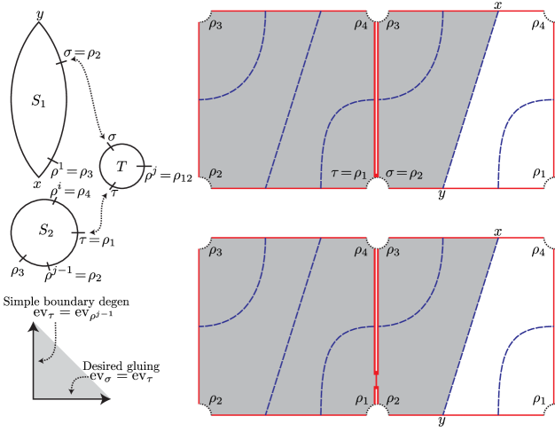
Figure 19. Gluing composite boundary degenerations. This is an example of the argument in Proposition 3.59. Near the composite boundary degeneration in the top row is a family of simple boundary degenerations. Gluing them gives a two-parameter family of curves, parameterized by the locations of the two boundary branch points in the lower-right figure. The desired gluings of the composite boundary degeneration are the boundary of this space where one cut has shrunk, i.e., $\operatorname{ev}_{\sigma}=\operatorname{ev}_{\tau}$.

Instead of gluing $u_{1}$, $u_{2}$, and $v$ together directly, we will consider gluing $u_{1}$ to a family of simple boundary degenerations near $T$ and see $(u_{1},u_{2},v)$ as an end of a family arising that way, via Lemma 3.58. The argument is illustrated in Figure 19.

After translating in $\mathbb{R}$, we can assume that $u_{1}$ is asymptotic to $\sigma$ at the point $(1,0)\in[0,1]\times\mathbb{R}$. Then, for small enough $\epsilon$, for each $t\in(0,\epsilon)$, by Lemma 3.48 and Proposition 4.5 there is a simple boundary degeneration $u_{t}$ through the points $(\pi_{\mathbb{D}}\circ u_{1})^{-1}(1,t)$ homotopic to $u_{2}$. By Proposition 3.57 we can glue $u_{1}$ to $u_{t}$. This gives a two-parameter family of curves $u_{s,t}$ where $s$ is the gluing parameter. The algebra asymptotics of $u_{s,t}$ are $(a_{1},\dots,a_{j-1},c,b,a_{j+1},\dots,a_{n})$.

Consider the compactification of the moduli space containing the $u_{s,t}$. We have two functions from this compactified moduli space to $\mathbb{R}_{+}$: the difference in $\mathbb{R}$-coordinates $\operatorname{ev}_{c}-\operatorname{ev}_{a_{j-1}}$ and the difference in $\mathbb{R}$-coordinates $\operatorname{ev}_{b}-\operatorname{ev}_{c}$. The product of these maps is a map to the first quadrant $\mathbb{R}_{+}^{2}$. By considering the possible limits, this map to $\mathbb{R}_{+}^{2}$ is proper near the origin. The subspace with $\operatorname{ev}_{c}-\operatorname{ev}_{a_{j-1}}=0$ corresponds to the simple boundary degenerations $(u_{1},u_{t})$, so maps by a degree $1$ map to the positive $y$-axis. So, by Lemma 3.58 the map to $\mathbb{R}_{+}^{2}$ is locally degree $1$ near the origin. Hence, the restriction to the subspace where $\operatorname{ev}_{b}-\operatorname{ev}_{c}=0$ is also degree $1$ near the origin; but points in this subspace are the desired gluing of the composite boundary degeneration. ∎

3.7. Compactness and the codimension-1 boundary

We now have all the tools needed to prove Theorem 1.12. Before doing so, we note that the counts used to define $\widehat{\mathit{CFA}}$ are finite:

Lemma 3.60.

Fix generators $\mathbf{x}$ and $\mathbf{y}$, $B\in\pi_{2}(\mathbf{x},\mathbf{y})$, a sequence of algebra elements $\vec{a}$, and an integer $w$, so that $\operatorname{ind}(B,\vec{a},w)=1$. Then, for any tailored family of almost complex structures $J$, the moduli space $\mathcal{M}^{B}(\mathbf{x},\mathbf{y};\vec{a};w)$ has finitely many elements.

Proof of Lemma 3.60 and Theorem 1.12.

Fix $\mathbf{x}$, $\mathbf{y}$, $B$, $\vec{a}$, and $w$ as in the statement of Lemma 3.60 so that $\operatorname{ind}(B,\vec{a},w)\leq 1$ for Lemma 3.60 and $2$ for Theorem 1.12 Fix also a decorated source ${S^{\mspace{1.0mu}\triangleright}}$ with corresponding sequence of algebra elements $\vec{a}$ and $w$ Reeb orbits, and such that $\chi(S)=\chi_{{\mathrm{emb}}}(B,\vec{a},w)$.

Step 1. The general structure of the limit. Consider a sequence of holomorphic polygons $u_{n}$, with respect to almost complex structures $J(P_{i})$ for some sequence of $P_{i}$. By compactness of $\mathfrak{M}$ (which is a quotient of the Deligne-Mumford moduli space), there is a subsequence so that the $P_{i}$ converge to some (possibly broken) polygon $P_{\infty}\in\mathfrak{M}$. Write the components of $P_{\infty}$ as $P_{\infty,1},\dots,P_{\infty,m}$. From the definition of a coherent family of admissible almost complex structures, the $J(P_{i})$ for that subsequence converge to $J(P_{\infty})$. The argument from ordinary bordered Floer homology [LOT18, Proposition 5.23], which boils down to applying symplectic field theory compactness first to the $\pi_{P}\circ u_{n}$, then to $\pi_{\Sigma}\circ u_{n}$ in a neighborhood of the puncture, and then to the $u_{n}$ on the complement of a smaller neighborhood, gives a convergent subsequence of the $u_{n}$. The limit has one component for each $P_{\infty,i}$ ($i=1,\dots,m$); these come in six kinds:

• Main components, which are maps to $\Sigma\times P_{\infty,i}$ where $P_{\infty,i}$ is a module component. In particular, part of the boundary of these components is mapped to ${\boldsymbol{\beta}}\times\{0\}\times\mathbb{R}$.

• Boundary degeneration components, which are maps to $\Sigma\times P_{\infty,i}$ where $P_{\infty,i}$ is an algebra polygon. In particular, all of the boundary of these components is mapped to ${\boldsymbol{\alpha}}\times\partial P_{\infty,i}$.

• $E\infty$ components, which are mapped to $(\mathbb{R}\times\partial\Sigma)\times P_{\infty,i}$.

• Fake $e\infty$ components, which are mapped to $\Sigma\times P_{\infty,i}$ where the map to $\Sigma$ is constant (which is necessarily to a point on $\alpha_{1}^{a}\cup\alpha_{2}^{a}$). (This happens, for instance, if a pair of boundary marked points labeled $U^{a}$ and $U^{b}$ collide; see the discussion of fake split curves in Section 3.2.3.) Below, we will abuse terminology and also refer to these as components at $e\infty$, because they play the same role in the argument.

• Disk bubbles, which are maps to $\Sigma\times P_{\infty,i}$ so that the map to $P_{\infty,i}$ is a constant map to the boundary while in $\Sigma$ all of the boundary of the component is mapped to one of $\alpha_{1}^{a}\cup{\boldsymbol{\alpha}}^{c}$, $\alpha_{2}^{a}\cup{\boldsymbol{\alpha}}^{c}$, or ${\boldsymbol{\beta}}$.

• Sphere bubbles, which have no boundary and are mapped to $P_{\infty,i}$ by a constant map.

These components are glued together by a gluing graph, whose vertices correspond to the components and whose edges indicate how the components intersect or, more accurately, are glued together in $u_{n_{i}}$ for $i\gg 0$. It follows from boundary monotonicity (or, essentially equivalently, from the symmetric product formulation in Section 3.2.5) that this gluing graph is, in fact, a tree (compare [LOT18, Lemma 5.57]). There are also some other degenerations which we can immediately see do not occur. Pairs of simple Reeb orbits colliding has codimension $2$ (see Formula 3.22 or 3.30). Formation of interior nodes (collapsing circles in the source $S$) also has codimension $2$: this increases $\chi$ by $2$, so decreases Formula 3.22 by $2$. Arcs in $S$ collapsing to form nodes without splitting at $\pm\infty$ or $e\infty$ or creating a boundary degeneration violates strong boundary monotonicity, as in the $\widehat{\mathit{HF}}$ case [LOT18, Lemma 5.50].

Step 2. Applying the index formula. Consider a broken holomorphic curve with a main component $u_{0}$ (which may be broken at $\pm\infty$), boundary degenerations $u_{1},\dots,u_{b}$, and $e\infty$ components $v_{1},\dots,v_{c}$, where $v_{1},\dots,v_{c}$ have a total of $m$ $w\infty$ algebra elements and $w^{\prime}$ $w\infty$ Reeb orbits, with total ramification $r$ (of the Reeb orbits). Recall that there are $k$ algebra elements and $w$ simple Reeb orbits at (far) east $\infty$. After gluing together these components, we have

$$\operatorname{ind}(B,{S^{\mspace{1.0mu}\triangleright}},\vec{a};w,0) =g-\chi(S)+2e(B)+k+w\leq 1\text{ or }2$$

$$\chi(S) =\chi(S_{0})+\cdots+\chi(S_{b})-bg$$

$$e(B) =e(B_{0})+e(B_{1})+\cdots+e(B_{b}).$$

Thus,

$$\operatorname{ind}(B_{0},{S_{0}^{\mspace{1.0mu}\triangleright}},\vec{a}_{0};w_{0},0)+\operatorname{ind}(B_{1},S^{\mspace{1.0mu}{\Box}}_{1},\vec{a}_{1};w_{1},0)+\cdots+\operatorname{ind}(B_{b},S^{\mspace{1.0mu}{\Box}}_{b},\vec{a}_{b};w_{b},0)\\ +k-m+w-w^{\prime}+r\leq 1\text{ or }2.$$

By Lemma 3.41, each $\operatorname{ind}(B_{i},S^{\mspace{1.0mu}{\Box}}_{i},\vec{a}_{i};w_{i},0)$, $i>0$, is at least $2$, and since the gluing graph is a tree, $k-m\geq-b$. Since Reeb orbits are never created (though they can collide or hit the boundary and turn into chords via orbit curves), $w-w^{\prime}\geq 0$ and, in fact, $w-w^{\prime}\geq r\geq 0$. Also, $\operatorname{ind}(B_{0},{S_{0}^{\mspace{1.0mu}\triangleright}},\vec{a}_{0};w_{0},0)\geq 0$. Thus, the left side is bounded below by $2b-b$, so $b\leq 1$ or $2$.

Step 3. Classifying the possibilities in the index $1$ case. In the index $1$ case, $b\leq 1$. If $b=1$ then we must have $\operatorname{ind}(B_{0},{S_{0}^{\mspace{1.0mu}\triangleright}},\vec{a}_{0};w_{0},0)=0$, so in fact $u_{0}$ is constant. Then, the curve consists of a single boundary degeneration, which has index at least $2$, a contradiction. If $b=0$ then $\operatorname{ind}(B_{0},{S_{0}^{\mspace{1.0mu}\triangleright}},\vec{a}_{0};w_{0},0)=1$ so $k-m=0$ and $w-w^{\prime}+r=0$. Thus, there are also no curves at $e\infty$ so the limit is an element of $\mathcal{M}^{B}(\mathbf{x},\mathbf{y};{S^{\mspace{1.0mu}\triangleright}})$, not a broken holomorphic curve. This proves Lemma 3.60.

Step 4. Classifying the possibilities in the index $2$ case. In the index $2$ case, the remaining possibilities are:

• $\operatorname{ind}(B_{0},{S_{0}^{\mspace{1.0mu}\triangleright}},\vec{a}_{0};w_{0},0)=2$, $b=0$, $k=m$, and $w=w^{\prime}$. In this case, there are no boundary degenerations or curves at $e\infty$. So, there are the following subcases:

  • A 2-story holomorphic building.

  • A constant map and a sphere bubble.

  • A constant map and a disk bubble.

  The latter two kinds of ends do not contribute to the count by properties (TJ-4) and (TJ-5) of the definition of a tailored family of almost complex structures, and Lemma 3.46.

• $\operatorname{ind}(B_{0},{S_{0}^{\mspace{1.0mu}\triangleright}},\vec{a}_{0};w_{0},0)=1$, $b=0$, $k=m+1$, and $w=w^{\prime}$. This corresponds to degenerating a split curve or a pseudo split curve at $e\infty$, or to a fake split curve; all of these cases are collision ends. (This uses the fact that if $b=0$ no component at $e\infty$ can have more than one $w\infty$ chord.)

• $\operatorname{ind}(B_{0},{S_{0}^{\mspace{1.0mu}\triangleright}},\vec{a}_{0};w_{0},0)=1$, $b=0$, $k=m$, and $w=w^{\prime}+1$. This corresponds to degenerating an orbit curve. (In particular, we must have $r=0$.)

• $\operatorname{ind}(B_{0},{S_{0}^{\mspace{1.0mu}\triangleright}},\vec{a}_{0};w_{0},0)=1$, $b=1$, $k=m-1$, and $w=w^{\prime}$. This corresponds to a composite boundary degeneration. (Again, this uses the fact that the gluing graph is a tree to rule out more complicated components at $e\infty$.)

• $\operatorname{ind}(B_{0},{S_{0}^{\mspace{1.0mu}\triangleright}},\vec{a}_{0};w_{0},0)=0$, $b=1$, $k=m$, and $w=w^{\prime}$. In this case, the main component is constant, so in particular has no algebra elements on it. Thus, since the gluing graph is a tree, there are no components at $e\infty$, either. Thus, this case corresponds to a simple boundary degeneration, connected to a constant main component.

• $\operatorname{ind}(B_{0},{S_{0}^{\mspace{1.0mu}\triangleright}},\vec{a}_{0};w_{0},0)=0$, $b=0$, $k=m$, and $w=w^{\prime}+2$ or $w=w^{\prime}+1$ and $r=1$. These cases are excluded by the same reasoning as the previous case.

• $\operatorname{ind}(B_{0},{S_{0}^{\mspace{1.0mu}\triangleright}},\vec{a}_{0};w_{0},0)=0$, $b=2$, $k=m-2$, and $w=w^{\prime}$. This is prohibited by the fact that the gluing graph is a tree.

So, we have shown that the degenerations which can contribute are of the types specified in the theorem. Conversely, Propositions 3.53, 3.54, 3.55, 3.56, 3.57, and 3.59 show that each of these degenerations does occur (with multiplicity one). ∎

4. The algebra of boundary degenerations

Let $\Sigma$ be a surface of genus $g$. For each energy $E$, fix a complex structure $j_{E}$ on $\Sigma$ which is regular for energy $E$ boundary degenerations, in the sense of Definition 3.47. The counts from Definition 3.49 can be organized into a weighted $A_{\infty}$-algebra, as follows.

Definition 4.1.

Let $\mathcal{A}=\mathcal{A}_{-}^{0,\mathrm{as}}$ be the associative algebra from Section 1.1.2. The multiplication is an operation $\mu_{2}^{0}\nobreak\mskip 2.0mu\mathpunct{}\nonscript\mkern-3.0mu{:}\penalty 300\mskip 6.0mu plus 1.0mu\mathcal{A}\otimes\mathcal{A}\to\mathcal{A}$. Define

$$\mu_{0}^{1}=\rho_{1234}+\rho_{2341}+\rho_{3412}+\rho_{4123}$$

and for $w>1$ let $\mu_{0}^{w}=0$. For non-negative integers $(w,n)$ with $n+2w>2$ and $n\geq 1$, let $\mu_{n}^{w}\nobreak\mskip 2.0mu\mathpunct{}\nonscript\mkern-3.0mu{:}\penalty 300\mskip 6.0mu plus 1.0mu\mathcal{A}[U]^{\otimes n}\to\mathcal{A}[U]$ be the map characterized by

(4.2) $$\begin{split}\mu_{n}^{w}(a_{1},\dots,a_{n})&=\#\mathcal{N}([\alpha_{i}^{a}];a_{1},\dots,a_{n};w)\iota_{i}U^{n_{z}+m}\\ &+\sum_{\begin{subarray}{c}a_{1}=\rho b\\ \operatorname{ind^{\square}}(b,a_{2},\dots,a_{n},w)=2\end{subarray}}\#\mathcal{N}([\alpha_{i}^{a}];b,a_{2},\dots,a_{n};w)\rho U^{n_{z}+m}\\ &+\sum_{\begin{subarray}{c}a_{n}=b\rho\\ \operatorname{ind^{\square}}(a_{1},\dots,a_{n-1},b,w)=2\end{subarray}}\#\mathcal{N}([\alpha_{i}^{a}];a_{1},a_{2},\dots,a_{n-1},b;w)\rho U^{n_{z}+m}\end{split}$$

where the first term only occurs if $\operatorname{ind^{\square}}(\vec{a},w)=2$, and the moduli spaces are defined by using $J_{E(a_{1},\dots,a_{n},w)}$ (cf. Formula (3.8)). In each case, the $\alpha$-arc $\alpha_{i}^{a}$ is determined by the sequence of algebra elements (which must be Reeby for the moduli space to be non-empty, by Lemma 3.41). The number $n_{z}$ is the degree with which the curve covers $z$, i.e., the degree of the map to $\Sigma$, and $m$ is the total $U$-power in $a_{1},\dots,a_{n}$.

We call $(\mathcal{A}[U],\{\mu_{n}^{w}\})$ the algebra associated to $\Sigma$ and $\{j_{E}\}$.

Our aim in this section is to prove the following precise form of Theorem 1.5:

Theorem 4.3.

For any energy $E$, there exists a choice of regular $j_{E}$ for energy $E$, in the sense of Definition 3.47. Moreover, for any such choices $j_{E}$, the operations $\mu^{w}_{n}$ in Definition 4.1 coincide with the weighted $A_{\infty}$-algebra associated to the torus, as defined in [LOT21].

In particular, Theorem 4.3 implies that the operations are $U$-equivariant, or equivalently the counts of the moduli spaces satisfy

(4.4) $$\#\mathcal{N}([\alpha_{i}^{a}];U^{i_{1}}\rho^{1},\dots,U^{i_{n}}\rho^{n};w)=\#\mathcal{N}([\alpha_{i}^{a}];\rho^{1},\dots,\rho^{n};w).$$

In Equation (4.2) of Definition 4.1, the last two sums on the right correspond to counting composite boundary degenerations, according to the following:

Proposition 4.5.

Fix a regular $j$, a non-negative integer $w$, a sequence basic algebra elements $\vec{a}=(a_{1},\dots,a_{n})$ so that $\operatorname{ind^{\square}}(\vec{a},w)=2$, and a factorization $a_{1}=bc$. For a generic tuple $\mathbf{w}=\{w_{i}\in\alpha_{i}^{c}\cap\beta_{\sigma(i)}\}$, the space of composite boundary degenerations $\#\mathcal{N}(b;a_{1},\dots,a_{n};w)$ asymptotic to $b\times\mathbf{w}$ is transversely cut out, and the count of simple boundary degenerations $\#\mathcal{N}([\alpha_{i}^{a}];c,a_{2},\dots,a_{n};w)$ agrees modulo 2 with the count of composite boundary degenerations $\#\mathcal{N}(b;a_{1},\dots,a_{n};w)$. (As usual, $\alpha_{i}^{a}$ is determined by the other data.)

A similar statement holds for boundary degenerations of the form $\mathcal{N}([\alpha_{i}^{a}];a_{1},\dots,a_{n-1},b;w)$ for any factorization $a_{n}=bc$.

Theorem 4.3 follows from the following assertions, verified below:

1. The holomorphic curve counts $\#\mathcal{N}([\alpha_{i}^{a}];\vec{a};w)$ are independent of the choice of regular $j$.

2. There are choices of $j$ that are regular.

3. The holomorphic curve counts are independent of the choice of genus $g$ or, equivalently, the choice of Heegaard surface $\Sigma$.

4. If $g=1$, the holomorphic curve counts agree with the coefficients in the weighted $A_{\infty}$ operations for the torus algebra $\mathcal{A}_{-}$ as defined combinatorially in our previous paper [LOT21].

Remark 4.6.

It follows that the operations $\mu^{w}_{n}$ endow $\mathcal{A}$ with the structure of a weighted $A_{\infty}$-algebra. This could be proved directly using the compactification of the spaces of pseudo-holomorphic curves, in the spirit of Section 5; but this is not necessary, in view of the identification from Step (a-4), since a combinatorial proof of the $A_{\infty}$-relations for the torus algebra is given in [LOT21, Theorem LABEL:TA:thm:AinftyAlgebra].

As a step towards establishing (a-1), we set up a suitable generalization of the complex structures used on $\Sigma\times\mathbb{H}$ and study boundary degenerations for this generalization. This is done in Section 4.1. We then verify (a-4) in Section 4.2. (This is almost immediate from the definition of $\mathcal{A}_{-}$.) The theorem then follows quickly from the stabilization invariance of boundary degeneration counts, which is proved in Section 4.3.

The $\beta$-circles on the bordered Heegaard diagram are irrelevant to the moduli spaces considered in this section. So, we will typically fix a partial Heegaard diagram $(\Sigma,{\boldsymbol{\alpha}})$ consisting of a compact, connected, oriented surface $\Sigma$ with some genus $g$ and one boundary component, $g-1$ circles $\alpha_{1}^{c},\dots,\alpha_{g-1}^{c}$, two arcs $\alpha_{1}^{a},\alpha_{2}^{a}$ with boundary on $\partial\Sigma$, and a basepoint $z\in\partial\Sigma$, so that the $\alpha$ arcs and circles are pairwise disjoint and linearly independent in $H_{1}(\Sigma,\partial\Sigma)$ and $z$ is just before one of the endpoints of $\alpha_{1}^{a}$ with respect to the orientation of $\partial\Sigma$. As usual, we will also use $\Sigma$ to denote $\Sigma\setminus\partial\Sigma$, which we view as a punctured Riemann surface, and $\alpha_{i}^{c}$ to denote the corresponding non-compact arc in this punctured surface. In particular, moduli spaces of holomorphic curves mean curves in this punctured Riemann surface, not the surface with boundary.

4.1. Generalized boundary degenerations

To establish (a-1), we need to generalize somewhat the almost complex structures we allow on $\Sigma\times\mathbb{H}$, beyond those considered in Section 3.2.4.

Definition 4.7.

An almost complex structure $J$ on $\Sigma\times\mathbb{H}$ is admissible to energy $E_{0}$ if it satisfies the following conditions:

1. The projection map $\pi_{\mathbb{H}}\nobreak\mskip 2.0mu\mathpunct{}\nonscript\mkern-3.0mu{:}\penalty 300\mskip 6.0mu plus 1.0mu\Sigma\times\mathbb{H}\to\mathbb{H}$ is $J$-holomorphic.

2. For each $(p,\zeta)\in\Sigma\times\mathbb{H}$, $J$ preserves the tangent space $T_{\zeta}\mathbb{H}\subset T_{(p,\zeta)}(\Sigma\times\mathbb{H})$.

3. The complex structure is split, as $j_{\Sigma}\times j_{\mathbb{D}}$, over a neighborhood of the puncture of $\Sigma$.

4. Each of the complex structures on $\Sigma\times\{\zeta\}$ induced by $J$ is $\eta(E_{0})$-pinched in the sense of Definition 3.3, for a sufficient pinching function $\eta$ (Definition 3.42).

Sufficiently pinched product complex structures on $\Sigma\times\mathbb{H}$ are admissible. For an admissible complex structure $J$, we can formulate the notion of boundary degenerations analogous to Definition 3.19, with the additional condition:

1. If $\vec{a}=(a_{1},\dots,a_{n})$ is the sequence of basic algebra elements $u$ is asymptotic to, then $u$ is asymptotic to $a_{1}$ at $(1,0)\in\partial\mathbb{H}$ and to $a_{2}$ at $(1,1)\in\partial\mathbb{H}$.

(If $J$ splits as a product $j_{\Sigma}\times j_{\mathbb{H}}$, this condition is equivalent to dividing out by the action of the (two-dimensional) group of conformal automorphisms of $\mathbb{H}$. For non-split $J$, the conformal group no longer acts holomorphically.) These more general boundary degenerations can be collected into moduli spaces, which we denote $\mathcal{N}(J;\mathbf{x};\vec{a};w)$, and then used to define operations $\mu_{n}^{w}$ associated to $\Sigma$ and $J$, immediately generalizing Definition 4.1. As in the split case, let

$$\mathcal{N}(J;*;\vec{a};w)=\bigcup_{\mathbf{x}}\mathcal{N}(J;\mathbf{x};\vec{a};w).$$

Also as in the split case, let

$$\mathcal{N}(J;[\alpha_{i}^{a}];\vec{a};w)$$

be the preimage of a regular value of the evaluation map from $\mathcal{N}(J;*;\vec{a};w)$ to $\alpha_{i}^{a}$ (where, as usual, $\alpha_{i}^{a}$ is the $\alpha$-arc containing the initial endpoint of $a_{1}$ and the terminal endpoint of $a_{n}$).

For admissible almost complex structures, we have the following transversality package, which is also the key step in proving that the count of $\mathcal{N}(J;[\alpha_{i}^{a}];\vec{a};w)$ is well-defined:

Theorem 4.8.

For a generic $J$ which is admissible to energy $E_{0}$, if $E(\vec{a},w)\leq E_{0}$ then the moduli spaces $\mathcal{N}(J;*;\vec{a};w)$ with

$$\operatorname{ind^{\square}}(\vec{a},w)\leq 2$$

are manifolds of dimension $\operatorname{ind^{\square}}(\vec{a},w)+g-2$. Further, any two such generic $J_{1}$ and $J_{2}$ can be connected by a path $\{J_{t}\}_{t\in[1,2]}$ so that the moduli spaces

$$\mathcal{N}(\{J_{t}\};*;\vec{a};w)\coloneqq\bigcup_{t\in[1,2]}\mathcal{N}(J_{t};*;\vec{a};w)$$

is a manifold-with-boundary, of dimension $\operatorname{ind^{\square}}(\vec{a},w)+g-1$.

We call almost complex structures as in the first part of Theorem 4.8 regular.

Proof.

The proof is similar to the proof of Proposition 3.50 and is left to the reader. ∎

Remark 4.9.

Although Theorem 4.8 establishes the existence of admissible almost complex structures $J$ that are regular, in a sense analogous to Definition 3.47, these $J$ need not be split. The fact that we can take $J$ to be split will be established in Section 4.3.

From Theorem 4.8, we conclude the following:

Proposition 4.10.

Consider a sequence of basic algebra elements $\vec{a}$ and an integer $w$ so that $\operatorname{ind^{\square}}(\vec{a},w)=2$. Then, for any regular $J$ the moduli space $\mathcal{N}(J;[\alpha_{i}^{a}];\vec{a};k)$ consists of finitely many points, and the modulo-2 count $\#(\mathcal{N}(J;[\alpha_{i}^{a}];\vec{a};w))$ is independent of the choice of regular, admissible (to energy $E(\vec{a},w)$) $J$.

Proof.

Both statements reduce to compactness results. For finiteness, by a similar argument to the proof of Lemma 3.48, the evaluation map $\operatorname{ev}\nobreak\mskip 2.0mu\mathpunct{}\nonscript\mkern-3.0mu{:}\penalty 300\mskip 6.0mu plus 1.0mu\mathcal{N}(J;*;\vec{a};k)\to\alpha_{i}^{a}$ is proper, and hence the preimage of any point, i.e., $\mathcal{N}(J;[\alpha_{i}^{a}];\vec{a};k)$, is compact. For the second statement, if $J_{1}$ and $J_{2}$ are both regular, we connect them by a regular path $\{J_{t}\}_{t\in[1,2]}$ in the sense of Theorem 4.8, so the resulting moduli space $\mathcal{N}(\{J_{t}\};*;\vec{a};w)$ is a manifold-with-boundary. By a similar argument to the proof of Lemma 3.48 (the key step in which is Lemma 3.41), the space $\mathcal{N}(\{J_{t}\};*;\vec{a};w)$ is compact. The evaluation map extends continuously to $\mathcal{N}(\{J_{t}\};*;\vec{a};w)$. Hence, its degree restricted to $t=1$ coincides with its degree restricted to $t=2$; i.e.,

$$\#\mathcal{N}(J_{1};[\alpha_{i}^{a}];\vec{a};w)=\#\mathcal{N}(J_{2};[\alpha_{i}^{a}];\vec{a};w),$$

as desired. ∎

Proposition 4.10 implies that the moduli spaces are $U$-equivariant, in the sense of Formula (4.4), since the $U$-powers in the algebra elements only affect the moduli spaces through which complex structures are considered. So, for the rest of the section, it will suffice to consider moduli spaces $\#\mathcal{N}(J;[\alpha_{i}^{a}];\rho^{1},\rho^{2},\dots,\rho^{n};w)$ where the asymptotics are Reeb chords.

4.2. The genus-one case

In [LOT21], we gave several definitions of a weighted $A_{\infty}$-algebra $\mathcal{A}_{-}(T^{2})$; we recall the one which is most directly connected with the pseudo-holomorphic curves. For this section, it suffices to consider only split complex structures on $\Sigma\times\mathbb{H}$, as in Section 3.2.4, not the more general admissible almost complex structures of Definition 4.7. (See also Proposition 4.11 below.)

As usual, equip the torus $T^{2}$ with two embedded curves $\alpha_{1}^{a}$ and $\alpha_{2}^{a}$ that intersect in a single, transverse intersection point $p$, i.e., the result of collapsing the dotted circle in the left or middle of Figure 1. The operations in the algebra count maps $f\nobreak\mskip 2.0mu\mathpunct{}\nonscript\mkern-3.0mu{:}\penalty 300\mskip 6.0mu plus 1.0mu\Delta\to T^{2}$ of the disk to the torus with the following properties:

• The boundary of the disk is mapped to $\alpha_{1}^{a}\cup\alpha_{2}^{a}$.

• The map $f$ is an immersion except for possible branching at points of $\partial\Delta$ that map to $p$.

In the operations, the weight $w$ counts the number of preimages of $p$ in the interior of $\Delta$, and the sequence of algebra elements corresponds to the corners around $p$, in the cyclic order they appear along $\partial\Delta$. Equivalently, the operations count tilings of the disk by squares marked as on the left of Figure 1, where the tiling is arranged so that exactly four tiles meet at each corner in the interior of $\Delta$.

Counts of such maps can be given an explicit, combinatorial description in terms of planar graphs, as in our previous paper [LOT21]. (See especially [LOT21, Section LABEL:TA:subsec:Immersions] for the correspondence between the two points of view.)

Proposition 4.11.

When $g=1$, any choice of complex structure $j$ on $\Sigma$ is regular, and the operations $\{\mu^{w}_{n}\nobreak\mskip 2.0mu\mathpunct{}\nonscript\mkern-3.0mu{:}\penalty 300\mskip 6.0mu plus 1.0mu\mathcal{A}^{\otimes n}\to\mathcal{A}[U]\}$ coincide with the weighted operations for $\mathcal{A}_{-}$. In particular, the operations $\mu^{w}_{n}$ make $\mathcal{A}[U]$ into a weighted algebra.

Proof.

Consider a boundary degeneration $u\nobreak\mskip 2.0mu\mathpunct{}\nonscript\mkern-3.0mu{:}\penalty 300\mskip 6.0mu plus 1.0muS\to\Sigma\times\mathbb{H}$. Since $g=1$, $\pi_{\mathbb{H}}\circ u$ is one-to-one, so $S$ is planar. The condition that $\operatorname{ind}(u)=2$ ensures that the branching of $f=\pi_{\Sigma}\circ u$ occurs at the punctures of $S$. Specifically, similar to the proof of Proposition 3.30, the Riemann-Hurwitz formula gives $1-w=\chi(S)=e(B)+|\vec{\rho}|/2-\operatorname{br}(u)$ where $B$ is the domain $\operatorname{br}(u)$ is the total ramification of $\pi_{\Sigma}\circ u$. If $B=k[\Sigma]$, this reduces to $1-w=-k+|\vec{\rho}|/2-\operatorname{br}(u)$. On the other hand, the index formula from Proposition (3.25) gives $2=1-\chi(S)-2k+|\vec{\rho}|+w$; since $\chi(S)=1-w$, this reduces to $2k+2=2w+|\vec{\rho}|$. Combining these two gives $\operatorname{br}(u)=0$.

The complex structure on $S$ is determined by the complex structure on $\Sigma$ and the branched cover $f$. This gives the one-to-one correspondence between the boundary degenerations counted in the $A_{\infty}$-algebra operations associated to the Heegaard surface with genus one (as in Definition 4.1) and the branched covers counted in the $A_{\infty}$-algebra operations in the torus algebra [LOT21].

Regularity of (any) $j$ follows, for instance, from the fact that the source curves are punctured disks and Hofer-Lizan-Sikorav’s automatic transversality argument [HLS97] (as in [LOT18, Proposition LABEL:LOT1:prop:east_transversality]). ∎

4.3. Stabilization invariance of boundary degeneration counts

The algebra associated to $\Sigma$ and $J$ was shown to be independent of $J$ in Proposition 4.10. In this section, we show that it is also independent of the Heegaard surface $\Sigma$. This is done by a familiar neck-stretching argument, analogous to the one from the cylindrical proof of stabilization invariance [Lip06, Section 12]. As in the forthcoming book on Heegaard Floer homology [OSS], we stabilize at two points rather than one, in the interest of technical simplicity; see Figure 20.

We will continue to work in the setting of admissible but not necessarily split almost complex structures, as in Definition 4.7. We require the almost complex structure to be split near the points where the stabilization occurs, in the following sense:

Definition 4.12.

Fix a finite set of points $\{p_{i}\}_{i=1}^{m}\subset\Sigma$. An admissible almost complex structure $J$ on $\Sigma\times\mathbb{H}$ is said to be product-like near $\{p_{i}\}_{i=1}^{m}$ if there is a neighborhood $D_{1}\amalg\dots\amalg D_{m}\subset\Sigma$ with $p_{i}\in D_{i}$, so that the restriction $J|_{(D_{1}\amalg\dots\amalg D_{m})\times\mathbb{H}}$ is split, as the product of a complex structure on $D_{i}$ and the standard complex structure on $\mathbb{H}$.

Definition 4.13.

Fix a partial Heegaard diagram $(\Sigma,{\boldsymbol{\alpha}})$ of genus $g$, points $z_{R}$ and $w_{R}$ in the interior of $\Sigma$, and an admissible almost complex structure which is product-like near $z_{R}$ and $w_{R}$. Fix also disjoint disk neighborhoods of $z_{R}$ and $w_{R}$ so that $J$ is split over these neighborhoods and a real parameter $T$. There is an associated almost complex structure $J(T)$ on the surface $\Sigma^{\prime}$ of genus $g+1$, obtained by attaching a cylinder with length $T$ to $\Sigma$ at the points $z_{R}$ and $w_{R}$, using the chosen disk neighborhoods. That is, if $D_{z}$ and $D_{w}$ are the chosen disks around $z_{R}$ and $w_{R}$, with some fixed identifications with the unit disk $D^{2}\subset\mathbb{C}$ (identifying $z_{R}$ and $w_{R}$ with the origin), then we build $(\Sigma^{\prime},J(T))$ by deleting the open disks of radius $1/2$ from $D_{z}$ and $D_{w}$ and gluing the complex cylinder $([0,\pi]\times[0,T/2])/(0,t)\sim(\pi,t)$ to the result by the canonical identifications. View $\Sigma^{\prime}$ as a partial Heegaard diagram via the $g+1$ curves from $\Sigma$, $\alpha_{1}^{a},\alpha_{2}^{a},\alpha_{1}^{c},\dots,\alpha_{g-1}^{c}$, and an additional circle $\alpha_{g}^{c}$ which contains one arc that runs through the attached cylinder as in Figure 20.

Note that the point $z_{R}$ in Definition 4.13 is different from the point $z$ in (or near) $\partial\Sigma$ in the definition of a Heegaard diagram.

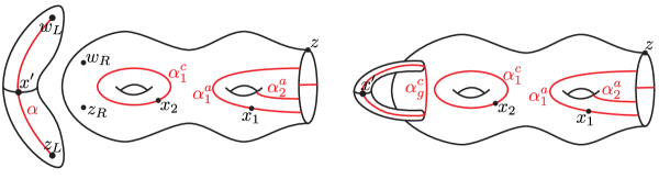
Figure 20. Stabilizing at two points. Left: the sphere $\mathbb{S}$ and the surface $\Sigma$. Right: the stabilized surface $\Sigma^{\prime}$, obtained by gluing $\Sigma$ and $\mathbb{S}$ at two points.

Fix a point $x^{\prime}\in\alpha_{g}$ which is at the center of the attached cylinder. Given $\mathbf{x}\in(\alpha^{a}_{1}\cup\alpha^{a}_{2})\times\alpha_{1}\times\dots\times\alpha_{g-1}$, there is an associated $\mathbf{x}^{\prime}\in(\alpha^{a}_{1}\cup\alpha^{a}_{2})\times\alpha_{1}\times\dots\times\alpha_{g-1}\times\alpha_{g}$ that agrees with $\mathbf{x}$ on the first $g$ factors, and whose component on $\alpha_{g}$ is $x^{\prime}$.

Let $\mathbb{S}$ denote the 2-sphere, and fix points $w_{L},z_{L}\in\mathbb{S}$ and an arc $\alpha\subset\mathbb{S}$ of a great circle connecting $w_{L}$ and $z_{L}$.

Definition 4.14.

Fix a point $x^{\prime}\in\alpha$. A stabilizing boundary degeneration at $x^{\prime}$ is a connected Riemann surface $S$ and a map $u\nobreak\mskip 2.0mu\mathpunct{}\nonscript\mkern-3.0mu{:}\penalty 300\mskip 6.0mu plus 1.0mu(S,\partial S)\to((\mathbb{S}\setminus\{z_{L},w_{L}\})\times\mathbb{H},\alpha\times\partial\mathbb{H})$ with the following properties:

• $S$ is equipped with a boundary puncture $q$ with the property that $u$ is asymptotic to $(x^{\prime},\infty)$ at $q$.

• $S$ is equipped with two more sets of interior punctures $\{w_{1},\dots,w_{k}\}$ and $\{z_{1},\dots,z_{k}\}$ so that $\pi_{\mathbb{S}}\circ u$ is asymptotic to the (simple) Reeb orbit around $z_{L}$ (respectively $w_{L}$) at $z_{i}$ (respectively $w_{i}$).

• The map $u$ is holomorphic, with respect to the split complex structure on $\mathbb{S}\times\mathbb{H}$ and some complex structure on $S$.

• The projection to $\mathbb{H}$, $\pi_{\mathbb{H}}\circ u$, has degree $1$. (In particular, $S$ is planar.)

Let $\mathcal{N}(x^{\prime};k)$ denote the moduli space of stabilizing boundary degenerations asymptotic to $x^{\prime}\in\alpha$.

The diagonal $\Delta\subset\operatorname{Sym}^{k}(\mathbb{H})$ consists of all elements $\mathbf{x}$ with a repeated entry. More generally, given a Cartesian product of symmetric products $(\operatorname{Sym}^{k}(\mathbb{H}))^{\times m}$, let $\Delta\subset(\operatorname{Sym}^{k}(\mathbb{H}))^{\times m}$ denote the diagonal consisting of those elements $\mathbf{x}_{1}\times\dots\times\mathbf{x}_{m}$ for which either some $\mathbf{x}_{i}$ has a repeated entry, or $\mathbf{x}_{i}\cap\mathbf{x}_{j}$ is nonempty, for some $i\neq j$. So, $\Delta$ is the preimage of the diagonal under the quotient map $(\operatorname{Sym}^{k}(\mathbb{H}))^{\times m}\to\operatorname{Sym}^{mk}(\mathbb{H})$.

There is an evaluation map $\operatorname{ev}\nobreak\mskip 2.0mu\mathpunct{}\nonscript\mkern-3.0mu{:}\penalty 300\mskip 6.0mu plus 1.0mu\mathcal{N}(x^{\prime};k)\to\operatorname{Sym}^{k}(\mathbb{H})\times\operatorname{Sym}^{k}(\mathbb{H})$ defined by

$$u\mapsto\Bigl{(}\bigl{\{}\pi_{\mathbb{H}}(u(z_{1})),\dots,\pi_{\mathbb{H}}(u(z_{k}))\bigr{\}},\bigl{\{}\pi_{\mathbb{H}}(u(w_{1})),\dots,\pi_{\mathbb{H}}(u(w_{k}))\bigr{\}}\Bigr{)}.$$

Lemma 4.15.

The evaluation map induces a proper map of degree $1$

$$\operatorname{ev}\nobreak\mskip 2.0mu\mathpunct{}\nonscript\mkern-3.0mu{:}\penalty 300\mskip 6.0mu plus 1.0mu\mathcal{N}(x^{\prime};k)\to\left(\operatorname{Sym}^{k}(\mathbb{H})\times\operatorname{Sym}^{k}(\mathbb{H})\right)\setminus\Delta.$$

In fact, the evaluation map is a diffeomorphism.

Proof.

We think of $\mathbb{S}$ as the one-point compactification of $\mathbb{C}$, so that $\alpha$ corresponds to $\mathbb{R}^{+}\cup\{\infty\}$, and $z_{L}$ and $w_{L}$ correspond to $0$ and $\infty$. (This uses the fact that $\alpha$ was an arc of a great circle.) Under this parameterization, the point $x^{\prime}$ corresponds to some real number $r>0$.

For notational simplicity, we also reparameterize the domain $\mathbb{H}$ by $\mathbb{H}^{+}=\{x+iy\mid y\geq 0\}$, so that the point at infinity in $\mathbb{H}$ corresponds to the origin $0\in\mathbb{H}^{+}$.

Curves in $\mathcal{N}(k,x^{\prime})$ correspond to holomorphic maps $f\colon\mathbb{H}^{+}\to\mathbb{C}$ satisfying:

• $f(\mathbb{R})\subset\mathbb{R}^{+}$; in fact, $f(\mathbb{R})$ is a closed interval in $\mathbb{R}^{+}$.

• $f(0)=r$.

• The poles and zeroes of $f$ do not occur on $\partial\mathbb{H}^{+}$.

• All of the poles and zeroes of $f$ are simple.

(The last condition corresponds to the condition that curves in $\mathcal{N}(k,x^{\prime})$ are required to be asymptotic to simple Reeb orbits.) After a Schwartz reflection, these in turn correspond to meromorphic (and hence rational) functions $F\colon\mathbb{C}\cup\{\infty\}\to\mathbb{C}\cup\{\infty\}$ with:

• $F(\mathbb{R})\subset\mathbb{R}^{+}$

• $F(0)=r$.

• There are no zeroes or poles of $F$ on $\mathbb{R}$.

• All of the zeros and poles of $F$ are simple.

Such functions are specified by their set of zeroes $Q\subset\mathbb{H}^{+}$ and poles $P\subset\mathbb{H}^{+}$ (all of which come in conjugate pairs, since they came from a Schwartz reflection), and a scaling parameter $\kappa$:

$$F(\zeta)=\kappa\left(\frac{\prod_{q\in Q}(\zeta-q)(\zeta-{\overline{q}})}{\prod_{p\in P}(\zeta-p)(\zeta-{\overline{p}})}\right);$$

where $\kappa$ is expressed in terms of $r$ (i.e. $x^{\prime}$) by

$$\kappa\cdot\left(\frac{\prod_{q\in Q}|q|}{\prod_{p\in P}|p|}\right)^{2}=r.$$

The image of the map $f$ under the evaluation map $\operatorname{ev}$ is the pair $(Q,P)$. Thus, $\operatorname{ev}$ induces a one-to-one correspondence. Since it is a continuous map between manifolds, it follows that $\operatorname{ev}$ is a homeomorphism.

To see that $\operatorname{ev}$ is a diffeomorphism, we argue as follows. The smooth structure on $\mathcal{N}(k,x^{\prime})$ agrees with the smooth structure induced on the rational functions in $\zeta\in\mathbb{C}$. Consider the map that associates to a rational function in $\zeta$ its (unordered) set of roots $Q$ and poles $P$. If none of those roots or poles is repeated, the Jacobian of the map is non-zero. ∎

Boundary degenerations in $\Sigma^{\prime}$ will be obtained by gluing boundary degenerations in $\Sigma$ to stabilizing boundary degenerations. To formulate this, we choose also two points $z_{R}$ and $w_{R}$ on $\Sigma$.

Proposition 4.16.

Fix an energy $E_{0}$. If $J$ is regular to energy $E_{0}$ and product-like near points $z^{\prime}_{R},w^{\prime}_{R}\in\Sigma$ and $z_{R}$ and $w_{R}$ are chosen generically in the neighborhoods of $z^{\prime}_{R}$ and $w^{\prime}_{R}$ where $J$ is split then for $T$ sufficiently large the associated complex structure $J(T)$ over $\Sigma^{\prime}$ is also regular to energy $E_{0}$. Moreover, for any $\vec{\rho}$ and $m$ with $E(\vec{\rho},m)\leq E_{0}$ and $\operatorname{ind^{\square}}(\vec{\rho},m)=2$,

$$\#\mathcal{N}(J;[\alpha_{i}];\rho^{1},\dots,\rho^{n};m)=\#\mathcal{N}(J(T);[\alpha_{i}];\rho^{1},\dots,\rho^{n};m).$$

Proof.

Since there are finitely many pairs $(\vec{\rho},m)$ with a given energy, it suffices to prove the result one tuple $(\vec{\rho},m)$ at a time. Fix a tuple of points $\mathbf{x}\in(\alpha_{1}^{a}\cup\alpha_{2}^{a})\times\alpha_{1}^{c}\times\dots\times\alpha_{g-1}^{c}$. Let $\{u_{T}\}$ be a sequence of curves in $\mathcal{N}(J(T);\mathbf{x}\times x_{0};\rho^{1},\dots,\rho^{n};m)$ with $T\to\infty$, with domain $k[\Sigma]$. By a compactness argument (similar to the proof of [LOT18, Proposition 5.24] or [LOT18, Proposition 9.6]), for a generic choice of $z_{R}$ and $w_{R}$, there is a subsequence of the $u_{T}$ which converges to a pair $(u_{L},v_{R})$ where:

• $u_{L}$ is a stabilizing boundary degeneration, in $\mathcal{N}(x^{\prime};k)$.

• $u_{R}\in\mathcal{N}(J;\mathbf{x};\rho^{1},\dots,\rho^{n};m)$.

• The $k$-tuple of points $(\pi_{\mathbb{H}}\circ u_{R})\bigl{(}(\pi_{\Sigma}\circ u_{R})^{-1}(z_{R})\bigr{)}$ agree with $\{(\pi_{\mathbb{H}}\circ u_{L})(\{w_{1},\dots,w_{k}\})$ and similarly the $k$-tuple of points $(\pi_{\mathbb{H}}\circ u_{R})\bigl{(}(\pi_{\Sigma}\circ u_{R})^{-1}(w_{R})\bigr{)}$ agree with $\{(\pi_{\mathbb{H}}\circ u_{L})(\{z_{1},\dots,z_{k}\})$.

In particular, the condition that $u_{L}$ has only simple Reeb orbits at $z_{L}$ is equivalent to the condition that $z_{R}$ is a regular value for $\pi_{\Sigma}\circ u_{R}$; by Sard’s theorem, generic $z_{R}$ and $w_{R}$ satisfy this condition. The fact that $u_{L}$ and $u_{R}$ meet only along orbits, not also Reeb chords, follows from elementary complex analysis: if they met along a Reeb chord, a maximum modulus theorem argument would imply that $\pi_{\mathbb{H}}\circ u_{R}$ is constant.

We claim that

$$\operatorname{ind}(u)=\operatorname{ind}(u_{T}).$$

Indeed, if we use a subscript $T$ to denote the terms in Formula (3.25) for $u_{T}$ then $g_{T}=g+1$ and $\chi_{T}=\chi+1-4k$, while the other terms are unchanged, giving the result. (Alternatively, the equality of indices also follows from Proposition 3.33.)

So, it follows from Lemma 3.41 that if $\operatorname{ind^{\square}}(\rho^{1},\dots,\rho^{n};m)\leq 1$ then the corresponding moduli space must be empty.

Assume next that $\operatorname{ind^{\square}}(\rho^{1},\dots,\rho^{n};m)=2$. It follows from standard gluing arguments (see the proof of [LOT18, Propositions 5.30 and 5.31] and the citations there) that for sufficiently large $T$, $\mathcal{N}(J(T),\mathbf{x}\times x_{0};\rho^{1},\dots,\rho^{n};m)$ is in the range of a gluing map from

$$\mathcal{N}(J;\mathbf{x};\rho^{1},\dots,\rho^{n};m)\times_{(\operatorname{Sym}^{k}(\mathbb{H})\times\operatorname{Sym}^{k}(\mathbb{H}))\setminus\Delta}\mathcal{N}(x^{\prime};k).$$

This uses the fact that the map $\mathcal{N}(J;\mathbf{x};\rho^{1},\dots,\rho^{n};m)\times\mathcal{N}(x^{\prime};k)\to\operatorname{Sym}^{m}(\mathbb{H})\times\operatorname{Sym}^{m}(\mathbb{H})$ in the definition of the fibered product is a submersion, which follows from Lemma 4.15. Further, since the map from the second factor is, in fact, a diffeomorphism, this fibered product is identified with its first factor. Thus, for $T$ large enough,

$$\mathcal{N}(J;\mathbf{x};\rho^{1},\dots,\rho^{n};m)\cong\mathcal{N}(J(T),\mathbf{x}\times x_{0};\rho^{1},\dots,\rho^{n};m),$$

as desired. ∎

Proof of Theorem 4.3.

This is an induction on the genus of $\Sigma$; the base case is Proposition 4.11, and the inductive step is provided by Proposition 4.16. ∎

Finally, we turn briefly to composite boundary, observing that the same argument shows that the counts of composite boundary degenerations are the same as the counts of simple ones (Proposition 4.5):

Proof of Proposition 4.5.

In the genus $1$ case, this follows from the description of boundary degenerations in Section 4.2: there is an obvious bijection between the two moduli spaces. (In the language of [LOT21], both correspond to the same tiling patterns.) The higher genus case then follows by the same degeneration argument that was used to prove Proposition 4.16. ∎

5. The module $\mathit{CFA}^{-}_{nu}$

In this section, we construct a version of the main invariant of 3-manifolds with torus boundary, the weighted $A_{\infty}$-module $\mathit{CFA}^{-}_{nu}(\mathcal{H})$, and prove it is independent of the choice of Heegaard diagram $\mathcal{H}$. The module $\mathit{CFA}^{-}_{nu}(\mathcal{H})$ has a mild algebraic defect: the actions on it are not $U$-equivariant. Remedying this defect requires one additional complication, which we discuss in Section 6. So, the ground ring for $\mathit{CFA}^{-}_{nu}(\mathcal{H})$ is ${\mathbb{F}_{2}}$, not ${\mathbb{F}_{2}}[U]$. On the other hand, if one is interested in studying ${\mathit{HF}}^{-}(Y)/(U^{n})$ for some $n$, the slightly simpler construction in this section suffices (for an appropriate choice of almost complex structures): one can arrange that the actions are $U$-equivariant up to any fixed order in $U$ (Remark 6.29). The grading on $\mathit{CFA}^{-}_{nu}$ is deferred to Section 7.

5.1. The definition of $\mathit{CFA}^{-}_{nu}$ as a weighted module

Fix a provincially admissible bordered Heegaard diagram $\mathcal{H}$.

The weighted $A_{\infty}$-module $\mathit{CFA}^{-}_{nu}(\mathcal{H})$ is the left ${\mathbb{F}_{2}}[U]$-module generated by $\mathfrak{S}(\mathcal{H})$, the set of generators for $\mathcal{H}$. The idempotents of $\mathcal{A}(\partial\mathcal{H})$ act on $\mathit{CFA}^{-}_{nu}(\mathcal{H})$ by $m_{2}^{0}(\mathbf{x},\iota_{i})=\mathbf{x}$ if $\mathbf{x}\cap\alpha_{i+1}^{a}\neq\emptyset$ and $m_{2}^{0}(\mathbf{x},\iota_{i})=0$ otherwise. (Recall that, for our conventions, $\iota_{0}$ corresponds to $\alpha_{1}^{a}$ and $\iota_{1}$ corresponds to $\alpha_{2}^{a}$.) We also define $m^{w}_{1+n}(\mathbf{x},a_{1},\dots,a_{n})=0$ for $n+2w>1$ if either $\iota_{i}\in\{a_{1},\dots,a_{n}\}$.

To define the rest of the weighted $A_{\infty}$-module structure, it suffices to specify the operation $m_{1+n}^{w}(\mathbf{x},a_{1},\dots,a_{n})$ for each $n$, $w$, and basic algebra sequence $(a_{1},\dots,a_{n})$, i.e., where each $a_{i}$ is of the form $U^{r_{i}}$ with $r_{i}\geq 1$ or $U^{r_{i}}\rho^{i}$ with $r_{i}\geq 0$ and $\rho^{i}$ some Reeb chord. Fix a tailored family of almost complex structures. Define

(5.1) $$m_{1+n}^{w}(\mathbf{x},a_{1},\dots,a_{n})=\sum_{\mathbf{y}\in\mathfrak{S}(\mathcal{H})}\sum_{\begin{subarray}{c}B\in\pi_{2}(\mathbf{x},\mathbf{y})\\ \operatorname{ind}(B;\rho_{1},\dots,\rho_{n};w)=1\end{subarray}}\#\mathcal{M}^{B}(\mathbf{x},\mathbf{y},a_{1},\dots,a_{n};w)U^{n_{z}(B)+\sum_{i=1}^{n}r_{i}}\mathbf{y}.$$

For this to make sense, we need the following:

Lemma 5.2.

Fix generators $\mathbf{x},\mathbf{y}\in\mathfrak{S}(\mathcal{H})$, basic algebra elements $a_{1},\dots,a_{n}$, and $w\in\mathbb{Z}$. Provincial admissibility of the bordered Heegaard diagram $\mathcal{H}$ implies that there are finitely many homology classes $B\in\pi_{2}(\mathbf{x},\mathbf{y})$ so that $\mathcal{M}^{B}(\mathbf{x},\mathbf{y};a_{1},\dots,a_{n};w)$ is non-empty. Further, given a tailored family of almost complex structures, if $\operatorname{ind}(B;a_{1},\dots,a_{n};w)=1$ then $\mathcal{M}^{B}(\mathbf{x},\mathbf{y};a_{1},\dots,a_{n};w)$ consists of finitely many points.

Proof.

This is a simple adaptation of the proof in the closed case [OSz04, Lemma 4.13] (see also [LOT18, Proposition 4.28]). If the moduli space is non-empty then the domain $B$ must have only non-negative coefficients. The sequence of chords $\rho^{i}$ corresponding to the $a_{i}$ and the integer $w$ determine the multiplicities of $B$ near $\partial\Sigma$. Consequently, any two such domains $B$ differ by a provincial periodic domain. Provincial admissibility implies that there is an area form on $\Sigma$ so that all provincial periodic domains have area $0$ [LOT18, Proposition 4.28]. In particular, all domains $B$ so that the moduli space is non-empty have the same area. There are only finitely many positive domains with a given area, so the result follows.

The finiteness statement is Lemma 3.60. ∎

Remark 5.3.

Since the basepoint $z$ is adjacent to the boundary, it follows that $m^{0}_{1}(\mathbf{x})$ is in the ${\mathbb{F}_{2}}$-span of ${\mathfrak{S}}(\mathcal{H})$; in particular, $H_{*}(\mathit{CFA}^{-}_{nu}(\mathcal{H}),m^{0}_{1})$ is a free (left) ${\mathbb{F}_{2}}[U]$-module.

As mentioned in the introduction, since $\pi_{2}(\mathbf{x},\mathbf{y})=\emptyset$ unless $\mathbf{x}$ and $\mathbf{y}$ represent the same $\operatorname{spin}^{c}$-structure (see Section 2), the module $\mathit{CFA}^{-}_{nu}(\mathcal{H})$ decomposes as a direct sum

$$\mathit{CFA}^{-}_{nu}(\mathcal{H})=\bigoplus_{\mathfrak{s}\in\operatorname{spin}^{c}(Y)}\mathit{CFA}^{-}_{nu}(\mathcal{H},\mathfrak{s}).$$

5.2. Proof of the structure equation

Recall that Theorem 1.11 states that $\mathit{CFA}^{-}_{nu}$ satisfies the weighted $A_{\infty}$-relations.

Proof of Theorem 1.11.

As usual, this follows by considering the ends of the $1$-dimensional moduli spaces, i.e., from Theorem 1.12. Consider the coefficient of $U^{m}\mathbf{y}$ in the weight $w$ $A_{\infty}$-relation with inputs $(\mathbf{x},a_{1},\cdots,a_{n})$. Since $\mathit{CFA}^{-}_{nu}$ is defined to be strictly unital, if any of the $a_{i}$ is an idempotent then verifying the weighted $A_{\infty}$-relation is straightforward, and is left to the reader. So, assume that all the $a_{i}$ are basic algebra elements. Then, this relation has the following kinds of terms:

1. Terms of the form $m_{1+n-j}^{w-w^{\prime}}\bigl{(}m_{1+j}^{w^{\prime}}(\mathbf{x},a_{1},\dots,a_{j}),a_{j+1},\dots,a_{n}\bigr{)}$. These are in bijection with terms of Type (e-1) in Theorem 1.12.

2. Terms of the form $m^{w}_{n}\bigl{(}\mathbf{x},a_{1},\dots,a_{j-1},\mu_{2}^{0}(a_{j},a_{j+1}),a_{j+2},\dots,a_{n}\bigr{)}$. These are in bijection with terms of Type (e-2) in Theorem 1.12.

3. Terms of the form $m_{2+n}^{w}\bigl{(}\mathbf{x},a_{1},\dots,a_{j},\mu_{0}^{1},a_{j+1},\dots,a_{n}\bigr{)}$. These are in bijection with terms of Type (e-3) in Theorem 1.12.

4. Terms of the form $m_{2+n-j}^{w-w^{\prime}}\Bigl{(}\mathbf{x},a_{1},\dots,a_{i},\mu_{j}^{w^{\prime}}\bigl{(}a_{i+1},\dots,a_{i+j}\bigr{)},a_{i+j+1},\dots,a_{n}\Bigr{)}$ where $j+2w^{\prime}>2$ and $j\geq 1$. There are two sub-cases:

   1. If $w-w^{\prime}=n-j=0$, these correspond to terms of Type (e-4) in Theorem 1.12.

   2. Otherwise, these correspond to terms of Type (e-5) in Theorem 1.12.

So, by Theorem 1.12, the coefficient of $U^{m}\mathbf{y}$ vanishes (modulo 2). ∎

5.3. Invariance under changes of almost complex structures and isotopies

In this section, we note invariance of $\mathit{CFA}^{-}_{nu}$ under isotopies and changes in the almost complex structure.

Proposition 5.4.

Fix a provincially admissible bordered Heegaard diagram $\mathcal{H}=(\Sigma,{\boldsymbol{\alpha}},{\boldsymbol{\beta}})$. If $J$ and $J^{\prime}$ are tailored families of almost complex structures then the modules $\mathit{CFA}^{-}_{nu}(\mathcal{H};J)$ and $\mathit{CFA}^{-}_{nu}(\mathcal{H};J^{\prime})$ computed with respect to $J$ and $J^{\prime}$ are $A_{\infty}$-homotopy equivalent.

Proof.

The proof is similar to the proof of the analogous result for $\widehat{\mathit{CFA}}$ [LOT18, Section 7.3.1] or ordinary Heegaard Floer homology [OSz04, Proposition 7.1], but with some superficial complications because we are considering families of almost complex structures.

Recall from Definition 3.1 that a bimodule component has two distinguished boundary punctures, labeled $\pm\infty$, and some other interior and boundary punctures labeled by energies. The $\pm\infty$ punctures divide the rest of the boundary into $\{0\}\times\mathbb{R}$ and $\{1\}\times\mathbb{R}$. A bimodule map component is defined similarly to a bimodule component, except with a third distinguished puncture, which we call $(1,0)$, along the edge $\{1\}\times\mathbb{R}$. There is a compactified moduli space $\mathfrak{BM}$ of bimodule map polygons, whose boundary points are trees with one vertex a bimodule map component and the other vertices bimodule components or algebra-type components. Given a point $P$ in the boundary of $\mathfrak{BM}$, each bimodule component of $P$ (if there are any) either comes above or below the bimodule map component. Call bimodule components top or bottom bimodule components in these two cases; see Figure 21.

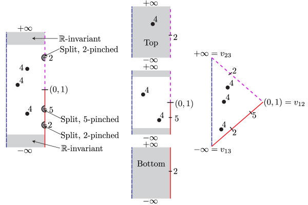
Figure 21. Bimodule map polygons. Left: a bimodule map component, drawn as $[0,1]\times\mathbb{R}$ with marked points, with some conditions on the almost complex structure marked. Center: a point in the boundary of $\mathfrak{BM}$, with a top bimodule component and a bottom bimodule component. Right: in Section 5.4, we will think of bimodule map polygons as triangles.

An interpolating tailored family of almost complex structures is a continuous family of almost complex structures $\widetilde{J}$ on $\Sigma\times P$ parameterized by $P\in\mathfrak{BM}$ so that

• Each $J(P)$ satisfies Conditions (J-1), (J-2), (J-3), (J-4)(J-4)(b), and (J-5) of the definition of an $\eta$-admissible almost complex structure (Definition 3.4), for some sufficient pinching function $\eta$, and preserves $\{x\}\times TP$ for each $x\in\Sigma$,

• $\widetilde{J}$ agrees with the $\mathbb{R}$-invariant almost complex structure $J^{\prime}_{\infty}$ specified by $J^{\prime}$ near $+\infty$ and with the $\mathbb{R}$-invariant almost complex structure $J_{\infty}$ specified by $J$ near $-\infty$,

• $\widetilde{J}$ agrees with $J^{\prime}$ over every top bimodule component, and with $J$ over every bottom bimodule component, and

• $\widetilde{J}$ satisfies the obvious analogue of the coherence condition (2) from Definition 3.6 over the bimodule map component, and

• $\widetilde{J}$ satisfies the obvious analogues of Conditions (TJ-1) (being sufficiently pinched), and (TJ-2) (the moduli spaces of main components being transversely cut out, up to index $1$), of a tailored family (Definition 3.51).

The proof that interpolating tailored families exist is similar to the proof of Corollary 3.52.

Given an interpolating tailored family $\widetilde{J}$, define moduli spaces $\mathcal{M}^{B}(\widetilde{J};\mathbf{x},\mathbf{y};\vec{a};w)$ as in Definition 3.14, but using $\widetilde{J}$. Note that, because of the extra puncture, these moduli spaces are one dimension larger than the moduli spaces $\mathcal{M}^{B}(\mathbf{x},\mathbf{y};\vec{a};w)$. Define $f^{w}_{1+n}\nobreak\mskip 2.0mu\mathpunct{}\nonscript\mkern-3.0mu{:}\penalty 300\mskip 6.0mu plus 1.0mu\mathit{CFA}^{-}_{nu}(\mathcal{H};J)\otimes\mathcal{A}_{-}^{\otimes n}\to\mathit{CFA}^{-}_{nu}(\mathcal{H};J^{\prime})$ by

$$f_{1+n}^{w}(\mathbf{x},a_{1},\dots,a_{n})=\sum_{\mathbf{y}\in\mathfrak{S}(\mathcal{H})}\sum_{\begin{subarray}{c}B\in\pi_{2}(\mathbf{x},\mathbf{y})\\ \operatorname{ind}(B;\vec{a};w)=0\end{subarray}}\#\mathcal{M}^{B}(\widetilde{J};\mathbf{x},\mathbf{y};\vec{a};w)U^{n_{z}(B)+m}\mathbf{y},$$

where $m$ is the sum of the $U$-powers in the elements of $\vec{a}$. The index-1 moduli spaces $\mathcal{M}^{B}(\widetilde{J};\mathbf{x},\mathbf{y};\vec{a};w)$ have ends corresponding to two-story buildings, collisions of levels, orbit curve degenerations, and composite boundary degenerations. (Simple boundary degenerations do not occur in index $1$ moduli spaces.) In the $(n+1)$-input, weight $w$ $A_{\infty}$-relation for $F=\{f_{1+m}^{v}\}$, these correspond to terms of the form

$$f_{1+m}^{v} (m_{1+n-m}^{w-v}(\mathbf{x},a_{1},\dots,a_{n-m}),a_{n-m+1},\dots,a_{n})\quad\text{and}$$

$$m_{1+m}^{v} (f_{1+n-m}^{w-v}(\mathbf{x},a_{1},\dots,a_{n-m}),a_{n-m+1},\dots,a_{n});$$

$$f_{n}^{w} (\mathbf{x},a_{1},\dots,a_{i}a_{i+1},\dots,a_{n});$$

$$f_{n+2}^{w-1} (\mathbf{x},a_{1},\dots,a_{i},\mu_{0}^{1},a_{i+1},\dots,a_{n});\quad\text{and}$$

$$f_{1+m}^{v} (\mathbf{x},a_{1},\dots,a_{i-1},\mu_{n-m+1}^{w-v}(a_{i},\dots,a_{i+n-m}),a_{i+n-m+1},\dots,a_{n})\quad\text{with $n-m+1>2$},$$

respectively. Compactness and gluing results for these index-1 moduli spaces follow as in Section 3.7. So, the number of ends is even, and the $f_{1+n}^{w}$ form a weighted $A_{\infty}$-module homomorphism.

Define a homomorphism $G=\{g_{1+n}^{w}\}$ from $\mathit{CFA}^{-}_{nu}(\mathcal{H};J^{\prime})$ to $\mathit{CFA}^{-}_{nu}(\mathcal{H};J)$ similarly, with the roles of $J$ and $J^{\prime}$ exchanged, using an interpolating tailored family of almost complex structures $\overline{J}$. Finally, to show that $G\circ F$ and $F\circ G$ are homotopic to the identity maps, consider a moduli space $\mathfrak{HM}$ bimodule homotopy polygons which have four distinguished marked points, two of which are in $\{1\}\times\mathbb{R}$, and corresponding families of almost complex structures on $\Sigma\times P$. One kind of boundary point of $\mathfrak{HM}$ occurs when the distance between the two distinguished points on $\{1\}\times\mathbb{R}$ goes to infinity; these ends are identified with pairs of bimodule map polygons, and correspond to $G\circ F$ (or $F\circ G$). Another end is where the two distinguished points on $\{1\}\times\mathbb{R}$ collide; identify these polygons with bimodule polygons by forgetting the extra pair of marked points. These ends then correspond to the identity map. Other ends of the space correspond to homotopy terms. ∎

Proposition 5.5.

If provincially admissible bordered Heegaard diagrams $\mathcal{H}=(\Sigma,{\boldsymbol{\alpha}},{\boldsymbol{\beta}})$ and $\mathcal{H}^{\prime}=(\Sigma,{\boldsymbol{\alpha}}^{\prime},{\boldsymbol{\beta}}^{\prime})$ differ by an isotopy of the $\alpha$- and $\beta$-curves then the modules $\mathit{CFA}^{-}_{nu}(\mathcal{H})$ and $\mathit{CFA}^{-}_{nu}(\mathcal{H}^{\prime})$ are $A_{\infty}$-homotopy equivalent.

Proof.

Again, the proof is similar to the case of $\widehat{\mathit{HF}}$, as well as to the proof of Proposition 5.4. It suffices to consider the case of a small Hamiltonian isotopy, where one defines chain maps by counting holomorphic curves as in the proof of Proposition 5.4, except now with varying boundary conditions instead of varying almost complex structures (compare, for example [Lip06, Section 9]). ∎

5.4. Handleslide invariance

The goal of this section is to prove:

Proposition 5.6.

Let $\mathcal{H}$ be a bordered Heegaard diagram, and $\mathcal{H}^{\prime}$ the result of performing a handleslide on $\mathcal{H}$, of one $\beta$-circle over another, one $\alpha$-circle over another, or an $\alpha$-arc over an $\alpha$-circle. Assume that both $\mathcal{H}$ and $\mathcal{H}^{\prime}$ are provincially admissible. Then $\mathit{CFA}^{-}_{nu}(\mathcal{H})\simeq\mathit{CFA}^{-}_{nu}(\mathcal{H}^{\prime})$.

The three cases in the proposition are similar, but there are some complications for $\alpha$-handleslides that do not occur for $\beta$-handleslides, and for $\alpha$-handleslides the case of sliding an arc over a circle is slightly more complicated than the case of sliding a circle. So, we will focus on that most complicated case and leave the others to the reader.

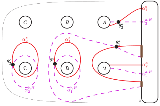
Figure 22. Handleslide curves. The two short Reeb chords connecting $\alpha_{1}^{a}$ and $\alpha_{1}^{a,H}$ are indicated by thick segments. This figure is adapted from [LOT18, Figure 6.3].

Write $\mathcal{H}=(\Sigma,{\boldsymbol{\alpha}},{\boldsymbol{\beta}})$ and $\mathcal{H}^{\prime}=(\Sigma,{\boldsymbol{\alpha}}^{H},{\boldsymbol{\beta}})$, where ${\boldsymbol{\alpha}}^{H}$ is obtained from ${\boldsymbol{\alpha}}$ by a handleslide. Like the case of $\widehat{\mathit{HF}}$, a quasi-isomorphism between $\mathit{CFA}^{-}_{nu}(\mathcal{H})$ and $\mathit{CFA}^{-}_{nu}(\mathcal{H}^{\prime})$ is constructed by counting pseudo-holomorphic triangles. We will consider the case of sliding $\alpha_{1}^{a}$ over $\alpha_{1}^{c}$; the case of sliding $\alpha_{2}^{a}$ over an $\alpha$-circle is identical. Choose the curves ${\boldsymbol{\alpha}}^{H}$ so that each circle $\alpha_{i}^{c,H}$ intersects $\alpha_{i}^{c}$ in two points and each $\alpha_{i}^{a,H}$ intersects $\alpha_{i}^{a}$ in one point, and all the $\alpha$-curves are disjoint other than this. Further require that there is a small triangle with boundary on $\partial\Sigma$, $\alpha_{1}^{a}$, and $\alpha_{1}^{a,H}$ (in that counter-clockwise order), and two small triangles with boundary on $\partial\Sigma$, $\alpha_{2}^{a}$, and $\alpha_{2}^{a,H}$. See Figure 22. For each $\alpha$-circle, there are two bigons with boundary on $(\alpha_{i}^{c},\alpha_{i}^{c,H})$ from one intersection point $\theta_{i}^{c}$ to the other point $\eta_{i}^{c}$. Let $\Theta_{1}$ (respectively $\Theta_{2}$) be the $g$-tuple of points in ${\boldsymbol{\alpha}}\cap{\boldsymbol{\alpha}}^{H}$ consisting of all the points $\theta_{i}^{c}$ and the unique point $\theta_{i}^{a}$ in $\alpha_{1}^{a}\cap\alpha_{1}^{a,H}$ (respectively $\alpha_{2}^{a}\cap\alpha_{2}^{a,H}$). (Roughly, the condition about the triangles with boundary on $\alpha_{i}^{a}$, $\alpha_{i}^{a,H}$, and $\partial\Sigma$ means that $\theta_{i}^{a}$ corresponds to the top-graded generator in a closed Heegaard diagram.)

We start by describing the families of almost complex structures we will use. Let $\mathfrak{BM}$ be the compactified moduli space of bimodule map polygons from the proof of Proposition 5.4. Let $\Delta$ be a disk with three boundary punctures. Label the edges of $\Delta$ as $e_{1},e_{2},e_{3}$ counter-clockwise, and let $v_{ij}$ be the puncture between $e_{i}$ and $e_{j}$. Given a bimodule map component, there is a unique biholomorphic identification of $P\setminus\{\infty,-\infty,(0,1)\}$ with $\Delta$. Fix tailored families of almost complex structures for $\mathcal{H}$ and $\mathcal{H}^{\prime}$. A tailored triangular family of almost complex structures is a family $J(P)$ of almost complex structures on $\Sigma\times P$ for $P\in\mathfrak{BM}$ such that:

1. Each $J(P)$ agrees with the $\mathbb{R}$-invariant almost complex structure for $\mathcal{H}$ in a neighborhood of $v_{13}$ and with the $\mathbb{R}$-invariant almost complex structure for $\mathcal{H}^{\prime}$ in a neighborhood of $v_{23}$.

2. The projection $\pi_{\Delta}$ is $J(P)$-holomorphic, and $J(P)$ preserves $\{x\}\times T\Delta$ for each $x\in\Sigma$.

3. $J$ is split near the puncture of $\Sigma$.

4. $J(P)$ is sufficiently pinched in the following sense. For each algebra puncture along $e_{1}$ (respectively $e_{2}$), each $J(P)$ is constant and sufficiently pinched for the diagram $\mathcal{H}$ (respectively $\mathcal{H}^{\prime}$) in an $\epsilon$-neighborhood of the puncture. (Here, the $\epsilon$-neighborhoods are with respect to a metric coming from identifying $\Delta$ with an unbounded, closed region in $\mathbb{C}$, e.g., $[-1,1]\times\mathbb{R}\cup\mathbb{R}_{>0}\times[-1,1]$.)

5. On the compactification of $\mathfrak{BM}$, for bimodule components at the bottom, $J(P)$ agrees with the chosen family for $\mathcal{H}$, and for bimodule components at the top $J(P)$ agrees with the chosen family for $\mathcal{H}^{\prime}$.

6. $\widetilde{J}$ satisfies the obvious analogue of the coherence condition from Definition 3.6 over the bimodule map component.

7. The moduli spaces considered below, including the boundary degenerations which occur in the proof of Proposition 5.6, are transversely cut out.

The proof that tailored triangular families exist is similar to the proof of Corollary 3.52. Note that the pinching conditions along $e_{1}$ and $e_{2}$ are different and incompatible; see Figure 23.

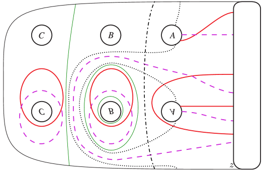
Figure 23. Pinching the almost complex structure for handleslides. The condition of being sufficiently $\epsilon$-pinched for ${\boldsymbol{\alpha}}$ requires pinching along the dot-dashed circle, near chords on $e_{1}$. The condition of being sufficiently pinched for ${\boldsymbol{\alpha}}^{H}$ requires pinching along the dotted circle, near chords on $e_{2}$. Note that these two pinchings cannot both be done at once, forcing the almost complex structure to be non-constant. For the proof of handleslide invariance we additionally pinch along the thin circles (denoted $C_{1}$, $C_{2}$, and $C_{3}$ in the proof of Lemma 5.9).

The chain homotopy equivalence

(5.7) $$f_{1+n}^{w}\nobreak\mskip 2.0mu\mathpunct{}\nonscript\mkern-3.0mu{:}\penalty 300\mskip 6.0mu plus 1.0mu\mathit{CFA}^{-}_{nu}(\mathcal{H})\otimes\mathcal{A}_{-}^{\otimes n}\to\mathit{CFA}^{-}_{nu}(\mathcal{H}^{\prime})$$

is defined by counting index-0 maps to $\Sigma\times\Delta$ with boundary on $({\boldsymbol{\alpha}}\times e_{1})\cup({\boldsymbol{\alpha}}^{H}\times e_{2})\cup({\boldsymbol{\beta}}\times e_{3})$, and asymptotic to $\Theta_{1}$ or $\Theta_{2}$ at $v_{12}$. (The analogue of $f$ was denoted $f^{{\boldsymbol{\alpha}},{\boldsymbol{\alpha}}^{H},{\boldsymbol{\beta}}}$ in [LOT18].) Let $\mathcal{M}^{B}(\mathbf{x},\mathbf{y},\Theta;\vec{a};w)$ denote the moduli spaces of such $J$-holomorphic curves, asymptotic to the sequence of basic algebra elements $\vec{a}$ along the edges $e_{1}\cup e_{2}$, and to $w$ orbits. Then

$$f_{1+n}^{w}(\mathbf{x},a_{1},\dots,a_{n})=\sum_{\mathbf{y},B}\#\mathcal{M}^{B}(\mathbf{x},\mathbf{y},\Theta;a_{1},\dots,a_{n};w)U^{n_{z}(B)+m}\mathbf{y}$$

where the sum is over homology classes $B$ of triangles so that the moduli space is $0$-dimensional, and $m$ is the number of factors of $U$ appearing in $a_{1},\dots,a_{n}$. This makes sense by analogues of Lemma 3.60 (so that every individual moduli space is compact) and Lemma 5.2 (so that the sum is finite).

In effect, we are using $\Theta_{i}$ as generators feeding into a triangle map. As in the closed case, to see that the induced map is a chain map (and, in our case, an $A_{\infty}$-homomorphism), one must check that $\Theta_{i}$ is a cycle in a suitable sense. In the closed case, this was the statement that finite energy flow lines out of $\Theta$ cancel in pairs. We formulate the analogous statement for the bordered case as follows.

Definition 5.8.

A generalized generator for the diagram $(\Sigma,{\boldsymbol{\alpha}}^{H},{\boldsymbol{\alpha}})$ consists of a $g$-tuple $\{x_{i}\}_{i=1}^{g}$, with $x_{i}\in\alpha^{c}_{i}\cap\alpha^{c,H}_{i}$ for $i=1,\dots,g-1$ and $x_{g}$ either the intersection point between $\alpha^{a}_{j}$ and $\alpha^{a,H}_{j}$ for $j\in 1,2$ or a Reeb chord with initial point on $\alpha^{a,H}_{j}$ and terminal point at $\alpha^{a}_{k}$.

Given generalized generators $\mathbf{x}$ and $\mathbf{y}$ for $(\Sigma,{\boldsymbol{\alpha}}^{H},{\boldsymbol{\alpha}})$, we will be interested in moduli spaces of embedded curves that connect then, labeled $\mathcal{M}^{B}(\mathbf{x},\mathbf{y};\vec{a},\vec{b};w)$. Here, $\vec{a}$ specifies the basic algebra elements for the $\alpha^{a,H}_{i}$ encountered over $\{1\}\times\mathbb{R}$; $\vec{b}$ specifies the basic algebra elements for $\alpha^{a}_{j}$ encountered over $\{0\}\times\mathbb{R}$; and $w$ specifies the number of Reeb orbits (all of which are required to be simple). To see that these moduli spaces are well behaved, recall that we require the almost complex structure to agree with the standard, split complex structure near the puncture in $\Sigma$. So, if we let $\overline{\Sigma}$ denote the result of filling in the puncture, by the removable singularities theorem any holomorphic curve in $\Sigma\times\Delta$ extends to a proper map to $\overline{\Sigma}\times\Delta$, where the generalized generators correspond to ordinary Heegaard Floer generators, and the usual Fredholm theory and compactness results for symplectic field theory apply. (If we do not fill in the puncture, the product of a neighborhood of the puncture with a neighborhood of $v_{23}$ is not a cylindrical end, but rather a product of two cylindrical ends and, as far as we know, the analytic underpinnings of pseudoholomorphic curves have not been developed in this setting.)

Lemma 5.9.

Fix $\ell\in\{1,2\}$. There exist tailored families of almost complex structures $J$ so that for any generalized generator $\mathbf{y}$, if $\mathcal{M}^{B}_{J}(\Theta_{\ell},\mathbf{y},\vec{a},\vec{b})$ is a non-empty, rigid moduli space then $n_{z}(B)=0$.

The complex structures used in the lemma are indicated in Figure 23. We postpone the proof of Lemma 5.9 to Section 5.4.1. Before that, we use it to deduce Proposition 5.6, and the following intermediate result:

Lemma 5.10.

For a family of almost complex structures as in Lemma 5.9, the map $f$ from Equation (5.7) is a homomorphism of weighted $A_{\infty}$ modules.

Proof.

A similar argument to the proof of Theorem 1.12 shows that the codimension-1 boundary of the space of holomorphic triangles has the following pieces:

1. Limits where the point in $\mathfrak{BM}$ consists of a pair of polygons, one a bimodule component containing $v_{13}$ and the other a bimodule map polygon component $v_{12}$ and $v_{23}$. These correspond to terms of the form

   $$f_{1+n}^{v}(m_{1+m}^{w}(\mathbf{x},a_{1},\dots,a_{m}),a_{m+1},\dots,a_{m+n}).$$

   (This includes the case that the component containing $v_{12}$ is a bigon.)

2. A pair of polygons, one a module map component containing $v_{12}$ and $v_{13}$ and the other a component containing $v_{23}$. These correspond to terms of the form

   $$m_{1+n}^{v}(f_{1+m}^{w}(\mathbf{x},a_{1},\dots,a_{m}),a_{m+1},\dots,a_{m+n}).$$

   (This includes the case that the component containing $v_{13}$ is a bigon.)

3. Limits where the point in $\mathfrak{BM}$ consists of a pair, or possibly a triple, of polygons, one a module map component containing all of $v_{12}$, $v_{23}$, and $v_{13}$ and a second one containing punctures and marked points on one of $e_{2}$ or $e_{3}$. In cases where the second component corresponds to a map to $e\infty$, there can be a third component that meets it, as with a composite boundary degeneration. These ends correspond to terms of the form

   $$f_{1+n}^{v}(\mathbf{x},a_{1},\dots,a_{i-1},\mu_{1+m}^{w}(a_{i},\dots,a_{i+m}),\dots,a_{m+n}).$$

   (This includes the case $m=-1$, which corresponds to an orbit curve end.)

4. Limits consisting of a module map component and a disk bubble with no interior or boundary punctures or marked points. There are algebraically zero ends of this form, because the count of disks with boundary on a single torus vanishes (Lemma 3.46) and standard gluing arguments.

5. Limits consisting of a module map component containing $v_{13}$ and $v_{23}$ and a polygon containing $v_{12}$.

(See Figure 24.)

Figure 24. Triangle degenerations. We have illustrated here four of the possible degenerations occurring for triangles in codimension one.

In more detail, the codimension one ends of the form (T-1) and (T-2) are analogous to the two-story buildings from Theorem 1.12. The fact that they each contribute with multiplicity $1$ follows from a straightforward adaptation of Proposition 3.53. Thus, the algebraic contributions of these ends to the one-dimensional moduli spaces are indeed

$$f_{1+n}^{v}(m_{1+m}^{w} (\mathbf{x},a_{1},\dots,a_{m}),a_{m+1},\dots,a_{m+n})$$ and

$$m_{1+n}^{v}(f_{1+m}^{w} (\mathbf{x},a_{1},\dots,a_{m}),a_{m+1},\dots,a_{m+n}),$$

as stated.

Type (T-3) ends can be classified: they can be collision ends (like Case (e-2) from Theorem 1.12), where one of the polygons is constant; they can correspond to an orbit curve degeneration (like Case (e-3)), where the degenerating polygon is a 1-gon containing an orbit; or they can contain a configuration like Case (e-5) consisting of a holomorphic triangle with a composite boundary degeneration at one Reeb chord along $e_{1}$ or $e_{2}$.

The fact that only these kinds of Type (T-3) ends contribute follows from index calculations and the fact the complex structure is sufficiently pinched, as in the proof of Theorem 1.12; and the fact that each of these ends counts with multiplicity $1$ uses a straightforward adaptation of the gluing methods used there (cf. Propositions 3.53, 3.54, 3.55, 3.56, 3.57, and 3.59). Thus, the contribution of these ends of Type (T-3) is indeed

$$f_{1+n}^{v}(\mathbf{x},a_{1},\dots,a_{i-1},\mu_{1+m}^{w}(a_{i},\dots,a_{i+m}),\dots,a_{m+n}).$$

(Collision ends correspond to the case of $\mu_{2}^{0}$, orbit curve ends to $\mu_{0}^{1}$, and the remaining ends to $\mu_{m}^{w}$ for $m+2w>0$.)

As mentioned above, ends of type (T-4) do not contribute to the count. It remains to consider ends of Type (T-5), to prove that all non-trivial such ends cancel in pairs.

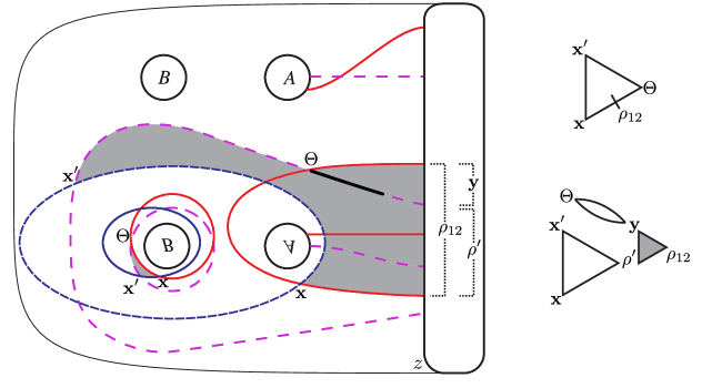
Figure 25. An end of type (T-5). On the left is a family of holomorphic triangles in the 1-dimensional moduli space $\mathcal{M}(\mathbf{x},\mathbf{x}^{\prime},\Theta;\rho_{12};)$, whose domain is shaded. As the thick cut approaches the boundary of $\Sigma$, a degeneration of Type (T-5) occurs. The components of the limit are indicated on the right; the shaded triangle is at $e\infty$.

The usual index considerations show that if the limit contains some component containing $v_{12}$, but not $v_{13}$ and $v_{23}$, then in fact that building consists of a rigid polygon containing $v_{13}$, $v_{23}$, and some chords and orbits, a rigid polygon containing $v_{12}$, in a $\mathcal{M}^{B}_{J_{\epsilon}}(\Theta_{\ell},\mathbf{y},\vec{a},\vec{b})$, for some sequence of chords $\vec{a}$ on ${\boldsymbol{\alpha}}$ and $\vec{b}$ on ${\boldsymbol{\alpha}}^{H}$ and some generalized generator $\mathbf{y}$, and perhaps a triangle at $e\infty$. (See Figure 25 for an example.) These moduli spaces could a priori contain quite complicated curves; for example, curves that cover the basepoint $z$. However, Lemma 5.9 ensures $n_{z}(B)=0$. Thus, these ends cancel in pairs exactly as they did in the $\widehat{\mathit{HF}}$ case [LOT18] (see for example [LOT18, Proposition 6.39]). ∎

Proof of Proposition 5.6.

The proof now follows using the same logic as in the case of bordered $\widehat{\mathit{HF}}$; [LOT18, Proposition 6.45] (which in turn is similar to the proof in the closed case [OSz04]), so we will be brief. Using $(\Sigma,{\boldsymbol{\alpha}}^{H},{\boldsymbol{\alpha}},{\boldsymbol{\beta}})$, we constructed a map by counting triangles $f\nobreak\mskip 2.0mu\mathpunct{}\nonscript\mkern-3.0mu{:}\penalty 300\mskip 6.0mu plus 1.0mu\mathit{CFA}^{-}_{nu}({\mathcal{H}}_{{\boldsymbol{\alpha}},{\boldsymbol{\beta}}})\to\mathit{CFA}^{-}_{nu}({\mathcal{H}}_{{\boldsymbol{\alpha}}^{H},{\boldsymbol{\beta}}})$, which we showed in Lemma 5.10 is a weighted $A_{\infty}$ homomorphism. Reverse the roles of ${\boldsymbol{\alpha}}^{H}$ and ${\boldsymbol{\alpha}}$ and displace the latter curves slightly to get a new set of curves ${\boldsymbol{\alpha}}^{\prime}$. Construct an analogous map $f^{\prime}\nobreak\mskip 2.0mu\mathpunct{}\nonscript\mkern-3.0mu{:}\penalty 300\mskip 6.0mu plus 1.0mu\mathit{CFA}^{-}_{nu}({\mathcal{H}}_{{\boldsymbol{\alpha}}^{H},{\boldsymbol{\beta}}})\to\mathit{CFA}^{-}_{nu}(\mathcal{H}_{{\boldsymbol{\alpha}}^{\prime},{\boldsymbol{\beta}}})$, which is a weighted homomorphism by the same reasoning. Counting quadrilaterals (compare [LOT18, Proposition 6.44]) now gives a weighted $A_{\infty}$-homotopy between the the composite

$$f^{\prime}\circ f\nobreak\mskip 2.0mu\mathpunct{}\nonscript\mkern-3.0mu{:}\penalty 300\mskip 6.0mu plus 1.0mu\mathit{CFA}^{-}_{nu}({\mathcal{H}}_{{\boldsymbol{\alpha}},{\boldsymbol{\beta}}})\to\mathit{CFA}^{-}_{nu}({\mathcal{H}}_{{\boldsymbol{\alpha}}^{\prime},{\boldsymbol{\beta}}})$$

and another triangle-counting map

$$\phi\nobreak\mskip 2.0mu\mathpunct{}\nonscript\mkern-3.0mu{:}\penalty 300\mskip 6.0mu plus 1.0mu\widehat{\mathit{CFA}}({\mathcal{H}}_{{\boldsymbol{\alpha}},{\boldsymbol{\beta}}})\to\widehat{\mathit{CFA}}({\mathcal{H}}_{{\boldsymbol{\alpha}}^{\prime},{\boldsymbol{\beta}}}),$$

associated to the triple $(\Sigma,{\boldsymbol{\alpha}},{\boldsymbol{\alpha}}^{\prime},{\boldsymbol{\beta}})$. (The fact that quadrilateral-counting furnishes a weighted $A_{\infty}$ chain homotopy uses an analogue of Lemma 5.9, which keeps algebra elements from escaping in ${\boldsymbol{\alpha}}^{H}$-${\boldsymbol{\alpha}}$ and ${\boldsymbol{\alpha}}^{H}$-${\boldsymbol{\alpha}}^{\prime}$ bigons.) We claim that the latter triangle-counting map $\phi$ is an isomorphism of weighted $A_{\infty}$ modules, which follows immediately once we show that $\phi^{0}_{1}\nobreak\mskip 2.0mu\mathpunct{}\nonscript\mkern-3.0mu{:}\penalty 300\mskip 6.0mu plus 1.0mu\mathit{CFA}^{-}_{nu}({\mathcal{H}}_{{\boldsymbol{\alpha}},{\boldsymbol{\beta}}})\to\mathit{CFA}^{-}_{nu}({\mathcal{H}}_{{\boldsymbol{\alpha}}^{\prime},{\boldsymbol{\beta}}})$ is an isomorphism of ${\mathbb{F}_{2}}[U]$-modules.

Setting $U=0$ in $\phi^{0}_{1}$, we obtain the isomorphism of $A_{\infty}$ modules $f^{{\boldsymbol{\alpha}},{\boldsymbol{\alpha}}^{\prime},{\boldsymbol{\beta}}}\nobreak\mskip 2.0mu\mathpunct{}\nonscript\mkern-3.0mu{:}\penalty 300\mskip 6.0mu plus 1.0mu\widehat{\mathit{CFA}}({\mathcal{H}}_{{\boldsymbol{\alpha}},{\boldsymbol{\beta}}})\to\widehat{\mathit{CFA}}({\mathcal{H}}_{{\boldsymbol{\alpha}}^{\prime},{\boldsymbol{\beta}}})$ from the $\widehat{\mathit{HF}}$ case [LOT18, Proof of Proposition 7.25], which we now denote $\widehat{\phi}^{0}_{1}$. Recall that our basepoints are on the boundary, so there is an isomorphism of chain complexes $\mathit{CFA}^{-}_{nu}({\mathcal{H}}_{{\boldsymbol{\alpha}},{\boldsymbol{\beta}}})\cong\widehat{\mathit{CFA}}({\mathcal{H}}_{{\boldsymbol{\alpha}},{\boldsymbol{\beta}}})\otimes_{{\mathbb{F}_{2}}}{\mathbb{F}_{2}}[U]$ and the map

$$\phi^{0}_{1}\nobreak\mskip 2.0mu\mathpunct{}\nonscript\mkern-3.0mu{:}\penalty 300\mskip 6.0mu plus 1.0mu\mathit{CFA}^{-}_{nu}({\mathcal{H}}_{{\boldsymbol{\alpha}},{\boldsymbol{\beta}}})\to\mathit{CFA}^{-}_{nu}({\mathcal{H}}_{{\boldsymbol{\alpha}}^{\prime},{\boldsymbol{\beta}}})$$

is induced from $\widehat{\phi}^{0}_{1}$ by a change of coefficients (i.e., tensoring with ${\mathbb{F}_{2}}[U]$). Since $\widehat{\phi}^{0}_{1}$ is an isomorphism of vector spaces [LOT18], it follows that $\phi^{0}_{1}$ is an isomorphism of ${\mathbb{F}_{2}}[U]$-modules. Hence, $f$ is a homotopy equivalence of weighted $A_{\infty}$-modules, as needed. ∎

5.4.1. Cancellation of flows out of $\Theta_{\ell}$

The aim of this section is to prove Lemma 5.9. To do this, we will find it convenient to consider first a diagram $\mathcal{H}^{0}$, whose Heegaard surface has genus one and one boundary component, equipped with two pairs of arcs ${\boldsymbol{\alpha}}^{\prime}=\{\alpha^{\prime}_{1},\alpha^{\prime}_{2}\}$ and ${\boldsymbol{\alpha}}=\{\alpha_{1},\alpha_{2}\}$. (We suppress the “a” superscript as there are no $\alpha$-circles.) Here, for $i=1,2$, $\alpha^{\prime}_{i}$ is a small isotopic translate of $\alpha_{i}$, translated against the boundary orientation, as shown in Figure 26.

Figure 26. The genus one diagram $\mathcal{H}^{0}$.

The Reeb chords $\rho_{i}$ connecting the endpoints in $\alpha_{1}\cup\alpha_{2}$ have analogous nearby copies, which we also denote $\rho_{i}$. For each $i=1,2$ there are two distinguished short chords from $\alpha^{\prime}_{i}$ to $\alpha_{i}$ which do not contain any points of $\partial\alpha^{\prime}_{j}$ or $\partial\alpha^{a}_{j}$ in their interior, and two distinguished small bigons $R^{a}_{i,1}$ and $R^{a}_{i,2}$ from $\theta_{i}^{a}$ to these four chords.

The natural analogues of generalized generators (Definition 5.8) are the intersection point $\theta_{1}^{a}$ of $\alpha_{1}$ with $\alpha_{1}^{\prime}$, the intersection point $\theta_{2}^{a}$ of $\alpha_{2}$ with $\alpha_{2}^{\prime}$, and any Reeb chord connecting some endpoint of $\alpha_{i}$ with $\alpha^{\prime}_{j}$.

We will be concerned with moduli spaces $\mathcal{M}^{B}(x,y;\vec{a},\vec{b};w)$, where $x\in\{\theta_{1}^{a},\theta_{2}^{a}\}$, $y$ is a generalized generator, $\vec{a}$ is a sequence of algebra elements whose Reeb chords connect endpoints of $\alpha_{1}\cup\alpha_{2}$, and $\vec{b}$ is a sequence of algebra elements whose Reeb chords connect endpoints of $\alpha_{1}^{\prime}\cup\alpha_{2}^{\prime}$. (The Reeb sequence $\vec{a}$ is listed in order of increasing $t$ parameter in $[0,1]\times\mathbb{R}$, while the sequence $\vec{b}$ is listed in decreasing $t$ parameter, as suggested by the boundary orientation on $[0,1]\times\mathbb{R}$.) Note that our curves have a degree $g=1$ projection to the bigon; in particular, the source curves all have genus $0$.

Example 5.11.

Consider the moduli space $\mathcal{M}^{B}(\theta_{1}^{a},\rho_{1}^{*};(\rho_{3},\rho_{23},\rho_{2}),(\rho_{41},\rho_{4});0)$, where $\rho_{1}^{*}$ is the generalized generator represented by the chord connecting $\alpha^{\prime}_{1}$ to $\alpha_{2}$ approximating $\rho_{1}$, and $B$ is the domain illustrated in Figure 27. This is a one-dimensional moduli space of disks (after dividing out by the usual $\mathbb{R}$ action) parameterized by a cut parameter at $\theta_{1}^{a}$.

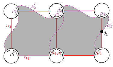
Figure 27. Disks out of $\theta_{1}^{a}$. The shaded domain $B$ can be represented by a one-dimensional (index two) moduli space of pseudo-holomorphic disks. Asymptotics are specified by $\mathcal{M}^{B}(\theta_{1}^{a},\rho_{1}^{*};\{\rho_{3},\rho_{23},\rho_{2}\},\{\rho_{41},\rho_{4}\})$.

Lemma 5.12.

Fix $\ell\in\{1,2\}$. Let $u$ be a non-constant holomorphic curve in some moduli space $\mathcal{M}^{B}(\theta_{\ell}^{a},y,\vec{a},\vec{b};w)$, and let $\operatorname{br}$ denote the number of branched points of the projection from $S$ to $[0,1]\times\mathbb{R}$. Suppose $m$ of the elements of $\vec{a}\cup\vec{b}$ are not Reeby (i.e., have the form $U^{i}\iota_{j}$). Then, $u$ lies in a moduli space with expected dimension given by

(5.13) $$\operatorname{ind}=1+2\operatorname{br}+m.$$

Proof.

The result is, effectively, about disks in the plane, and hence is standard [dSRS14]; nonetheless, we give a proof in the spirit of this present work, along the lines of the proof of Lemma 3.41. There are two slightly different cases, according to whether $y$ is an intersection point or a chord.

Each non-Reeby element adds one unconstrained marked point, hence increases the expected dimension by $1$. So, it suffices to prove the result when all of the chords are Reeby.

Assume first that it $y\in\{\theta_{1}^{a},\theta_{2}^{a}\}$. Analogous to the proof of Lemma 3.41, Proposition 3.22 gives

$$\operatorname{ind}(B,{S^{\mspace{1.0mu}\triangleright}},\vec{a},\vec{b},w,0)=1-\chi({S^{\mspace{1.0mu}\triangleright}})+2e(B)+|\vec{a}|+|\vec{b}|+w,$$

as in this case $g=1$; also, we are only considering the case of simple orbits, i.e., $r=0$, and drop $r$ from the notation. Let $k=n_{z}(B)$, so $e(B)=-k$. Since $\pi_{\mathbb{D}}\circ u$ is a $1$-fold cover, ${S^{\mspace{1.0mu}\triangleright}}$ has genus $0$, so

(5.14) $$\chi({S^{\mspace{1.0mu}\triangleright}})=1-w;$$

and we find that

(5.15) $$\operatorname{ind}(B,{S^{\mspace{1.0mu}\triangleright}},\vec{a},\vec{b},w,0)=1-(1-w)-2k+|\vec{a}|+|\vec{b}|+w=2w-2k+|\vec{a}|+|\vec{b}|.$$

We can compute $e({S^{\mspace{1.0mu}\triangleright}})$ either by projecting to the Heegaard surface, to find that

(5.16) $$e({S^{\mspace{1.0mu}\triangleright}})=-k-\operatorname{br};$$

or by comparing $e(S)$ with $\chi(S)$, via the formula

(5.17) $$e(S)=\chi(S)-|\vec{a}|/2-|\vec{b}|/2-1/2=1/2-w-|\vec{a}|/2-|\vec{b}|/2.$$

(The term $1/2$ comes from the two generators, each of which contributes $1/4$ to the Euler measure.) Equations (5.16) and (5.17) give

(5.18) $$-2k=2\operatorname{br}+1-2w-|\vec{a}|-|\vec{b}|.$$

Combining Equations (5.18) and (5.15) gives the result, Equation (5.13), in the case where $y$ is not a chord.

Next, consider the case that $y$ is a chord. In this case, $e(B)=-k+1/4$. The analogue of Proposition 3.22 is

(5.19) $$\operatorname{ind}(B,\theta_{1}^{a},y,{S^{\mspace{1.0mu}\triangleright}},\vec{a},\vec{b};w,0)=\frac{3}{2}-\chi({S^{\mspace{1.0mu}\triangleright}})+2e(B)+|\vec{a}|+|\vec{b}|+w.$$

(Note that in the reduction to the closed case, we must now glue one half-bigon, whose Euler measure is 1/4; i.e., following the proof of Proposition 3.22, we now glue a region $B^{\prime}$ with $e(B^{\prime})=e(B)+|\vec{a}|/2+|\vec{b}|/2+1/4$.) Equation (5.16) is replaced by

$$e({S^{\mspace{1.0mu}\triangleright}})=-k+1/4-\operatorname{br},$$

while Equation (5.17) remains unchanged. Equation (5.13) follows. ∎

Proposition 5.20.

Let $\ell\in\{1,2\}$. If $u$ is a pseudo-holomorphic curve in some rigid moduli space $\mathcal{M}^{B}(\theta_{\ell}^{a},y,\vec{a},\vec{b})$, then $u$ is one of the two small bigons from $\theta_{\ell}^{a}$ to the boundary. In particular the sequences $\vec{a}$ and $\vec{b}$ are empty, and $y$ is one of the two short Reeb chords connecting a point on the boundary of $\alpha_{1}$ to the corresponding point on the boundary of $\alpha^{\prime}_{1}$.

Proof.

By Lemma 5.12, our curve and all other curves in its moduli space have no branch points. Further, near the initial puncture, the curve is asymptotic to an arc connecting one of the two quadrants out of $\theta_{\ell}^{a}$ (since otherwise there is a curve in the same moduli space with a branch point). That quadrant is contained in one of the two distinguished small bigons $R^{a}_{1,j}$ out of $\theta_{1}^{a}$. In the rest of the proof we will show that the entire curve consists of that bigon. (This is clear, but we give a detailed argument.)

Let $U$ be a collar neighborhood of the boundary of the Heegaard surface, large enough to contain $R^{a}_{1,j}$. Equivalently, we can think of $U$ as a neighborhood of $p\in{\overline{\Sigma}}$. Foliate $U$ by concentric circles $\{C_{t}\}_{t\in(0,1]}$ around $p$, restricting to a foliation of $R^{a}_{1,j}$ by arcs. See Figure 28.

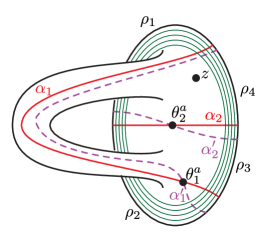
Figure 28. Foliation by circles. The foliation is indicated by the thin ellipses. The foliation continues until it covers $\theta_{1}^{a}$.

Take the preimage of this foliation to obtain a partial foliation on the source curve ${S^{\mspace{1.0mu}\triangleright}}$. (This foliation is defined only over $(\pi_{\Sigma}\circ u)^{-1}(U)$; as such, the foliation might not be defined near the $+\infty$ puncture of ${S^{\mspace{1.0mu}\triangleright}}$, provided that the latter is not labeled by a Reeb chord; but it is defined near all other punctures.) The asymptotics around each puncture ensure that the induced partial foliation is indeed a foliation around it by shrinking arcs. (See Figure 29.) The condition of no branching ensures that the foliation by concentric arcs around the initial vertex extends until the point where one of the concentric arcs hits another boundary puncture.

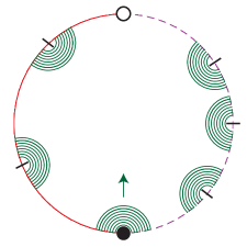
Figure 29. Induced foliation on the source. The initial puncture $(-\infty)$ is indicated by the black dot. The induced partial foliation is indicated by the thin arcs.

But these conditions exclude the existence of any boundary punctures other than the two at $\pm\infty$, which in turn ensures that $B=R^{a}_{1,j}$. ∎

With these preliminaries in place, we turn our attention to Lemma 5.9, which is proved by destabilizing to the genus $1$ case.

Proof of Lemma 5.9.

Fix a separating curve $C_{1}\subset\mathcal{H}$ so that the $\alpha_{i}^{a}$ and $\alpha_{i}^{a,H}$, $i=1,2$, and $\alpha_{1}^{c}$, and $\alpha_{1}^{c,H}$ are on one side of $C_{1}$, and the $\alpha_{j}^{c}$ and $\alpha_{j}^{c,H}$, $j=2,\dots,g-1$, are on the other side. Choose two more curves $C_{2}$, $C_{3}$ that together separate the $\alpha_{i}^{a}$ and $\alpha_{i}^{a,H}$ from $\alpha_{1}^{c}$ and $\alpha_{1}^{c,H}$. See Figure 23.

Let $J_{\epsilon}$ be a one-parameter family of tailored complex structures which are fixed outside a neighborhood of $C_{1}\cup C_{2}\cup C_{3}$ and so that a neighborhood of each $C_{i}$ is biholomorphic to $\{z\in\mathbb{C}\mid 1<|z|<1/\epsilon\}$. Taking Gromov limits of curves in $\mathcal{M}^{B}_{J_{\epsilon}}(\Theta_{\ell},\mathbf{y},\vec{a},\vec{b})$ as $\epsilon\to 0$ gives rise to a curve in $\mathcal{H}_{0}$. We will deduce topological properties of $B$ from the existence of these limits. For example, we will prove that if $\mathcal{M}^{B}_{J_{\epsilon}}(\Theta_{1},\mathbf{y},\vec{a},\vec{b})$ is a rigid moduli space which is non-empty for all sufficiently small $J_{\epsilon}$, then

(5.21) $$n_{z}(B)=0.$$

Figure 30. Regions in the handleslide diagram. The regions $R_{i,j}^{c}$ and $R_{i,j}^{1}$ are labeled. figure is also adapted from [LOT18, Figure 6.3].

In comparing the Heegaard diagram $\mathcal{H}$ with $\mathcal{H}_{0}$, note that $\mathcal{H}$ has $2g-2$ elementary domains not present in $\mathcal{H}_{0}$, corresponding to bigons connecting $\theta_{i}^{c}$ to $\eta_{i}^{c}$ with boundary on $\alpha_{i}^{c}\cup\alpha_{i}^{c,H}$. We label these domains $\{R^{c}_{i,1},R^{c}_{i,2}\}_{i=1,\dots,g-1}$; see Figure 30. Let $r^{c}_{i,j}$ denote the local multiplicity of $B$ at $R^{c}_{i,j}$ and let $k_{i,1}$ and $k_{i,2}$ denote the local multiplicities of $B$ at the other two regions adjacent to $\theta_{i}^{c}$. (Note that when $i\neq 1$, $k_{i,1}=k_{i,2}$, since the two regions are not separated by any $\alpha$ or $\alpha^{H}$ curve.) Let $J$ be the set of $i\in\{1,\dots,g-1\}$ for which $y_{i}\neq\theta^{c}_{i}$. For each $i\in\{1,\dots,g-1\}$, we have the relation

$$r^{c}_{i,1}+r^{c}_{i,2}=k_{i,1}+k_{i,2}+\begin{cases}1&{\text{if $i\in J$}}\\ 0&{\text{otherwise.}}\end{cases}$$

It follows that, if $K=\sum_{i=1}^{g-1}(k_{i,1}+k_{i,2})$ then

(5.22) $$\begin{split}e(B)&=e(B_{1})-K+{\textstyle\frac{1}{2}}|J|\\ n_{\Theta_{1}}(B)&=n_{\theta_{1}^{a}}(B_{1})+\frac{K}{2}+\frac{J}{4}\\ n_{\mathbf{y}}(B)&=n_{y}(B_{1})+\frac{K}{2}+\frac{J}{4}.\end{split}$$

The proof of the embedded index formula, Formula (3.32), using the tautological correspondence (Section 3.2.5) and Sarkar’s formula for the Maslov index of polygons in the symmetric product, applies equally well in this setting. So, by Formula (3.32),

(5.23) $$\operatorname{ind}(B,\Theta_{1},\mathbf{y},\vec{a},\vec{b},w,r)=\operatorname{ind}(B_{1},\theta_{1}^{a},y,\vec{a},\vec{b},w,r)+|J|.$$

Applying compactness to the sequence $u_{T}\in\widetilde{\mathcal{M}}^{B}_{J_{\epsilon}}(\Theta_{1},\mathbf{y},\vec{a},\vec{b})$ as $\epsilon\to 0$ gives rise to a holomorphic curve $u\in\widetilde{\mathcal{M}}^{B_{1}}(\theta_{1}^{a},y,\vec{a},\vec{b})$. (See also the proof of Lemma 3.41.) Since we assumed that $\operatorname{ind}(B,\Theta_{1},\mathbf{y},\vec{a},\vec{b},w,r)=1$, we can conclude from Lemma 5.12 that $|J|\leq 1$. If $|J|=1$, then $u$ is a constant curve, so $n_{z}(u)=0$. If $|J|=0$, then $u$ has index $1$, so Proposition 5.20 ensures that $n_{z}(B_{1})=0$. ∎

5.5. Stabilization invariance

Recall that by stabilizing a bordered Heegaard diagram $(\Sigma,{\boldsymbol{\alpha}},{\boldsymbol{\beta}})$ we mean taking the connected sum with the standard genus-one Heegaard diagram for $S^{3}$ at some point in the interior of $\Sigma\setminus({\boldsymbol{\alpha}}\cup{\boldsymbol{\beta}})$. (See [LOT18, Section 4.1] for more discussion.)

Proposition 5.24.

Let $\mathcal{H}=(\Sigma,{\boldsymbol{\alpha}},{\boldsymbol{\beta}})$ be a bordered Heegaard diagram and $\mathcal{H}^{\prime}=(\Sigma^{\prime},{\boldsymbol{\alpha}}^{\prime},{\boldsymbol{\beta}}^{\prime})$ the result of stabilizing $\mathcal{H}$. Then for appropriate choices of tailored almost complex structures for $\mathcal{H}$ and $\mathcal{H}^{\prime}$ there is an isomorphism of weighted $A_{\infty}$-modules $\mathit{CFA}^{-}_{nu}(\mathcal{H})\cong\mathit{CFA}^{-}_{nu}(\mathcal{H}^{\prime})$.

Proof.

This follows from the same argument as in Section 4.3 (which again is an extension of the usual proof of stabilization invariance for Heegaard Floer homology). The strategy is to show that for an appropriate choice of almost complex structures, the moduli spaces of holomorphic curves for $\mathcal{H}$ and $\mathcal{H}^{\prime}$ are identified. The almost complex structures for $\mathcal{H}^{\prime}$ are obtained by stretching the neck along a pair of curves. The amount of stretching required depends, at least in principle, on the moduli space being considered. So, the proof proceeds one energy level at a time, producing a complex structure $J_{E}$ for $\mathcal{H}$ and $J^{\prime}_{E}$ for $\mathcal{H}^{\prime}$ for which the rigid moduli spaces of energy $E$ holomorphic curves are identified, so that the $J_{E}$ and $J^{\prime}_{E}$ form tailored families.

Let $T\subset\Sigma^{\prime}$ be the new punctured torus, so $\Sigma^{\prime}\setminus T$ is identified with $\Sigma\setminus D^{2}$. Choose a tailored family of almost complex structures $J^{\prime}$ for $\mathcal{H}^{\prime}$ which is split over $T$. Let $\alpha_{g}^{c}\subset T$ be the new $\alpha$-circle and $\beta_{g+1}$ the new $\beta$-circle. Let $Z=Z_{1}\amalg Z_{2}\subset T$ be the boundary of a tubular neighborhood of $\alpha_{g}^{c}$, chosen so that each $Z_{i}$ intersects $\beta_{g+1}$ in a single point. We will stretch the neck along $Z_{1}$ and $Z_{2}$, after with $\Sigma^{\prime}$ degenerates into a copy of $\Sigma$ and a sphere $\mathbb{S}$. Let $z_{L}$, $w_{L}$ (respectively $z_{R}$, $w_{R}$) be the points in $\mathbb{S}$ (respectively $\Sigma$) corresponding to $Z_{1}$ and $Z_{2}$. Identify $\mathbb{S}$ with $\mathbb{C}\cup\{\infty\}$ so that $z_{L}$ corresponds to $0$ and $w_{L}$ corresponds to $\infty$. Using isotopy invariance, we may assume that $\alpha_{g}^{c}\cap\mathbb{S}$ is identified with the non-negative real axis $\mathbb{R}_{\geq 0}$ and $\beta_{g+1}$ is identified with the unit circle $S^{1}$. Also because of isotopy invariance, we will not distinguish between the copy of $\Sigma$ obtained by stretching the neck and the original copy in $\mathcal{H}$.

For a generic, sufficiently pinched choice of $J^{\prime}$, the family of almost complex structures $J$ in the limit is still tailored. (This uses the fact that the circle $Z$ is disjoint from the circle being pinched to make $J^{\prime}$ or $J$ sufficiently pinched.)

The proof is now inductive on the energy $E$. Assume that for all $\vec{a}$ and $w$ with $E(\vec{a},w)<E_{0}$ we have found a length $T$ so that the rigid moduli spaces with respect to $J_{T}$ and $J$ with asymptotics $(\vec{a},w)$ are identified. We will find a perhaps larger $T$ with this property for pairs $(\vec{a},w)$ with $E(\vec{a},w)=E_{0}$, and use this more stretched $J_{T}$ for energy $E_{0}$ moduli spaces (in our tailored family). There are finitely many $(\vec{a},w)$ with $E(\vec{a},w)=E_{0}$, and finitely many positive domains $B$ compatible with each $(\vec{a},w)$, so we may work one triple $(\vec{a},w,B)$, with $\operatorname{ind}(B,\vec{a},w)=1$, at a time. As we stretch the neck, a compactness argument (similar to the proof of [LOT18, Proposition 5.24] or [LOT18, Proposition 9.6]) implies that any sequence $\{u_{i}\}$ of $J_{T}$-holomorphic curves in the homology class $B$ with asymptotics $(\vec{a},w)$ has a subsequence which converges to a pair $(u_{L},u_{R})$ where

$$u_{L} \nobreak\mskip 2.0mu\mathpunct{}\nonscript\mkern-3.0mu{:}\penalty 300\mskip 6.0mu plus 1.0mu(S_{L},\partial S_{L})\to\bigl{(}(\mathbb{C}\cup\{\infty\})\times[0,1]\times\mathbb{R},\mathbb{R}_{\geq 0}\cup S^{1}\bigr{)}$$

$$u_{R} \nobreak\mskip 2.0mu\mathpunct{}\nonscript\mkern-3.0mu{:}\penalty 300\mskip 6.0mu plus 1.0mu(S_{R},\partial S_{R})\to\bigl{(}\Sigma\times[0,1]\times\mathbb{R},({\boldsymbol{\alpha}}\times\{1\}\times\mathbb{R})\cup({\boldsymbol{\beta}}\times\{0\}\times\mathbb{R})\bigr{)}.$$

(The curve $u_{L}$ is analogous to the stabilizing boundary degenerations of Definition 4.14.) Elementary complex analysis, considering $\pi_{\mathbb{D}}\circ u_{R}$, shows that in fact no component of $\partial S_{R}$ maps to $\alpha_{g}^{c}\cap\Sigma$. The pair $(u_{L},u_{R})$ also satisfies a matching condition: the multisets

$$A=(\pi_{\mathbb{D}}\circ u_{R})\bigl{(}(\pi_{\Sigma}\circ u_{R})^{-1}(z_{R})\bigr{)}\qquad\text{and}\qquad(\pi_{\mathbb{D}}\circ u_{L})\bigl{(}(\pi_{\mathbb{S}}\circ u_{L})^{-1}(z_{L})\bigr{)}$$

agree, as do the sets

$$B=(\pi_{\mathbb{D}}\circ u_{R})\bigl{(}(\pi_{\Sigma}\circ u_{R})^{-1}(w_{R})\bigr{)}\qquad\text{and}\qquad(\pi_{\mathbb{D}}\circ u_{L})\bigl{(}(\pi_{\mathbb{S}}\circ u_{L})^{-1}(w_{L})\bigr{)}.$$

In particular, the degree of $\pi_{\mathbb{S}}\circ u_{L}$ is the same as the multiplicity of the domain $B$ at $Z_{1}$ and $Z_{2}$.

It follows from the index formula (Proposition 3.30) that the index of the sequence converging to $(u_{L},u_{R})$ is the same as the index at $u_{R}$. In particular, since we are only interested in index-1 moduli spaces, $u_{R}$ is rigid. So, for a generic choice of almost complex structure, none of the points in $A$ or $B$ has multiplicity bigger than one, and $A\cap B=\emptyset$.

We claim that for each choice of $A$ and $B$, there is a unique curve $u_{L}$ satisfying the matching condition. The projection $\pi_{\mathbb{D}}\circ u_{L}$ is a degree-one branched cover, so an analytic isomorphism. So, the moduli space of maps $u_{L}$ is identified with the moduli space of maps from the strip to $\mathbb{S}$. Identify $[0,1]\times\mathbb{R}$ with the upper half-disk $\mathbb{D}^{+}=\{x+iy\in\mathbb{C}\mid x^{2}+y^{2}\leq 1,\ y\geq 0\}$ so that $\{1\}\times\mathbb{R}$ is identified with the real axis. This moduli space is the same as the space of holomorphic maps $\mathbb{D}^{+}\to\mathbb{C}$ sending the real axis to the positive real axis and the top semi-circle to $S^{1}$. By Schwartz reflecting (twice), this space is the same as the space of maps $f\nobreak\mskip 2.0mu\mathpunct{}\nonscript\mkern-3.0mu{:}\penalty 300\mskip 6.0mu plus 1.0mu\mathbb{C}P^{1}\to\mathbb{C}P^{1}$ with $f(S^{1})\subset S^{1}$ and $f(\mathbb{R})\subset\mathbb{R}_{>0}$. Up to an scaling by a complex number, such a function is determined by its zeroes and poles: given two entire functions $f,g$ with the same zeroes and poles, $f/g$ is an entire function with no zeroes (or poles), and hence is constant. The zeroes and poles satisfy the restrictions that zeroes (respectively poles) come in conjugate pairs (since $\mathbb{R}$ maps to $\mathbb{R}$) and zeroes correspond to poles under the map $z\mapsto 1/z$ (since $S^{1}$ maps to $S^{1}$). Thus, up to scaling, such a function is determined by its set of zeroes and poles inside $\mathbb{D}^{+}$. Again up to scaling, the condition that $f(\mathbb{R})\subset\mathbb{R}_{>0}$ (rather than just $\mathbb{R}$) is equivalent to $f$ having no zeroes or poles on $\mathbb{R}$. Finally, given a finite set $C\subset\mathbb{D}^{+}$, let $g_{C}$ be the Blaschke product

$$f_{C}(z)=\prod_{c\in C}\left(\frac{z-c}{1-\overline{c}z}\right).$$

Then given a set $Z$ of zeroes and $P$ of poles in the interior of $\mathbb{D}^{+}$ (with $Z\cap P=\emptyset$) the function $f_{Z}(z)/f_{P}(z)$ has the specified zeroes and poles. To summarize, given disjoint sets of zeroes and poles in the interior of $\mathbb{D}^{+}$, there is a unique function with these zeroes and poles.

Thus, for each curve $u_{R}$ there is a unique curve $u_{L}$ satisfying the matching condition. So, by a gluing argument, the space of holomorphic curves with respect to $J_{T}$ for $T$ sufficiently large is in bijection with the space of holomorphic curves $u_{R}$. Since the latter is exactly the space used to define the operations on $\mathit{CFA}^{-}_{nu}(\mathcal{H})$, and the former the operations on $\mathit{CFA}^{-}_{nu}(\mathcal{H}^{\prime})$, the result follows. ∎

5.6. The invariance theorem

We assemble these pieces to quickly deduce that $\mathit{CFA}^{-}_{nu}$ is well-defined; this is the analogue of Theorem 1.14 for $\mathit{CFA}^{-}_{nu}$:

Theorem 5.25.

Up homotopy equivalence (of weighted $A_{\infty}$-modules), $\mathit{CFA}^{-}_{nu}(\mathcal{H},\mathfrak{s})$ depends only on the bordered 3-manifold $(Y,\phi)$ specified by $\mathcal{H}$, and its underlying $\operatorname{spin}^{c}$ structure $\mathfrak{s}$.

Proof of Theorem 1.14.

Independence of the almost complex structure is Proposition 5.4. Next, any two bordered Heegaard diagrams representing the same bordered 3-manifold can be connected by a sequence of isotopies, handleslides over circles, and stabilizations [LOT18, Proposition 4.10], so this is immediate from Propositions, 5.5, 5.6, and 5.24. ∎

6. Grounding $U$

The aim of the present section is to modify the construction of $\mathit{CFA}^{-}_{nu}$ above to define a unital, weighted module $\mathit{CFA}^{-}(\mathcal{H})$ whose operations are $U$-equivariant (i.e., which is defined over the ground ring $\mathds{k}[U]=\mathds{k}\otimes{\mathbb{F}_{2}}[U]$).

We construct $\mathit{CFA}^{-}$ in three steps:

1. First, we define a larger weighted $A_{\infty}$-algebra $\mathcal{A}_{-}^{g}$, called the grounding algebra, equipped with a subalgebra $B\subset\mathcal{A}_{-}^{g}$ which is isomorphic, as a weighted $A_{\infty}$-algebra, to $\mathcal{A}_{-}$. (This isomorphism is not $U$-equivariant.) Thus, we can view $\mathit{CFA}^{-}_{nu}$ as a weighted $A_{\infty}$-module over $B$.

2. Next, we extend the actions on $\mathit{CFA}^{-}_{nu}$ in a $U$-equivariant way to all of $\mathcal{A}_{-}^{g}$, to construct a weighted module $\mathit{CFA}^{-}_{g}$ over $\mathcal{A}_{-}^{g}$.

3. There is a $U$-equivariant quasi-isomorphism $\mathcal{A}_{-}^{g}\simeq\mathcal{A}_{-}$. Restriction of scalars now allows us to turn any $\mathcal{A}_{-}^{g}$-module into a (quasi-isomorphic) $\mathcal{A}_{-}$-module. Applying this process to $\mathit{CFA}^{-}_{g}$ gives $\mathit{CFA}^{-}$.

6.1. The grounding algebra

Informally, $\mathcal{A}_{-}^{g}$ from Step (S-1) is obtained from $\mathcal{A}_{-}$ by adding elements $X$ and $e$, satisfying

$$d(X)=1+e\qquad{\text{and}}\qquad X^{2}=0,$$

and replacing the algebra operations that output $U^{n}$ (respectively $U^{n}\cdot\rho$) by operations that output $(Ue)^{n}$ (respectively $(Ue)^{n}\cdot\rho$).

More formally, the underlying algebra of $\mathcal{A}_{-}^{g}$ is obtained from the algebra underlying $\mathcal{A}_{-}^{0}$ by adjoining two commuting elements $e$ and $X$, subject to the relation $X^{2}=0$; i.e.,

$$A^{g}=\frac{{\mathbb{F}_{2}}[U,e,X]}{(X^{2})}\otimes_{\mathbb{F}_{2}}\mathcal{A}_{-}^{0,\mathrm{as}}.$$

Equip $A^{g}$ with the differential $\mu_{1}^{0}\nobreak\mskip 2.0mu\mathpunct{}\nonscript\mkern-3.0mu{:}\penalty 300\mskip 6.0mu plus 1.0muA^{g}\to A^{g}$ that vanishes on the subalgebra generated by $\mathcal{A}_{-}^{0,\mathrm{as}}$, $U$, and $e$, and that satisfies $\mu_{1}^{0}(X)=1+e$. Let $B\subset\mathcal{A}_{-}^{g}$ be the subalgebra generated by $U\cdot e$, $\rho_{1}$, $\rho_{2}$, $\rho_{3}$, and $\rho_{4}$.

There is an isomorphism of algebras $\phi\nobreak\mskip 2.0mu\mathpunct{}\nonscript\mkern-3.0mu{:}\penalty 300\mskip 6.0mu plus 1.0mu\mathcal{A}_{-}\to B$ characterized by the property that $\phi$ is the identity on $\mathcal{A}_{-}^{0,\mathrm{as}}$ and $\phi(U)=U\cdot e$. We can use this isomorphism to define weighted $A_{\infty}$ operations on $B$; explicitly, given a sequence $a_{1},\dots,a_{n}\in\mathcal{A}_{-}$, let

$$\mu^{w}_{n}(\phi(a_{1}),\dots,\phi(a_{n}))=\phi(\mu^{w}_{n}(a_{1},\dots,a_{n})).$$

We extend these operations to all of $\mathcal{A}_{-}^{g}$ as follows. The algebra $\mathcal{A}_{-}^{g}$ is generated by the subalgebra $B$, together with the elements $U$, $e$, and $X$. Extend the operations on $B$ to maps $\{\mu^{w}_{n}\nobreak\mskip 2.0mu\mathpunct{}\nonscript\mkern-3.0mu{:}\penalty 300\mskip 6.0mu plus 1.0mu(A^{g})^{\otimes n}\to A^{g}\}$ by the convention that all maps $\mu^{w}_{n}$ are equivariant under multiplication by $U$, $e$, and $X$. Since $\mu_{1}^{0}X=1+e$ is central, the resulting operations satisfies the weighted $A_{\infty}$ relations, giving $A^{g}$ the structure of weighted algebra $\mathcal{A}_{-}^{g}$, as desired. By construction $B\subset\mathcal{A}_{-}^{g}$ is a weighted $A_{\infty}$-subalgebra.

Example 6.1.

In $B\subset\mathcal{A}_{-}^{g}$, we have the operation

$$\mu^{0}_{4}(\rho_{4},\rho_{3},\rho_{2},\rho_{12})=\rho_{2}Ue.$$

This gives rise to further actions in $\mathcal{A}_{-}^{g}$, such as

$$\mu^{0}_{4}(\rho_{4},\rho_{3},X\cdot\rho_{2},e\cdot\rho_{12}) =X\rho_{2}Ue^{2}$$

$$\mu^{0}_{4}(\rho_{4},X\cdot\rho_{3},X\cdot\rho_{2},e\cdot\rho_{12}) =0.$$

The isomorphism $\phi\nobreak\mskip 2.0mu\mathpunct{}\nonscript\mkern-3.0mu{:}\penalty 300\mskip 6.0mu plus 1.0mu\mathcal{A}_{-}\to B$ allows us to view the module $\mathit{CFA}^{-}_{nu}$ as a weighted $A_{\infty}$-module over the $A_{\infty}$-subalgebra $B$, which we denote $\mathit{CFA}^{-}_{g}(\mathcal{H})|_{B}$. More formally:

Definition 6.2.

Given a provincially admissible bordered Heegaard diagram $\mathcal{H}$, the restricted module $\mathit{CFA}^{-}_{g}(\mathcal{H})|_{B}$ is defined as follows. As a left ${\mathbb{F}_{2}}[U]$-module it is freely generated by $\mathfrak{S}(\mathcal{H})$. The weight $w$ algebra operation on $\mathit{CFA}^{-}_{g}(\mathcal{H})|_{B}$ is specified on a generator $\mathbf{x}$ and a sequence of algebra elements $b_{1},\dots,b_{n-1}\in B$ as $m^{w}_{n}(\mathbf{x},\phi^{-1}(b_{1}),\dots,\phi^{-1}(b_{n-1}))$, where $m^{w}_{n}$ is the action on $\mathit{CFA}^{-}_{nu}$ defined in Section 5. That is, the action by $U^{n}e^{n}$ (respectively $U^{n}e^{n}\rho$) is identified with the action of $U^{n}$ (respectively $U^{n}\rho$) on $\mathit{CFA}^{-}_{nu}(\mathcal{H})$.

This completes Step (S-1) in our construction of $\mathit{CFA}^{-}$. Our next goal is to extend the restricted module $\mathit{CFA}^{-}_{g}(\mathcal{H})|_{B}$, defined over the weighted subalgebra $B\subset\mathcal{A}_{-}^{g}$, to one defined over all of $\mathcal{A}_{-}^{g}$. We do this in Section 6.4, after setting up some preliminaries about almost complex structures and moduli spaces.

Remark 6.3.

Unlike the operations on $\mathcal{A}_{-}^{g}$ itself, the action of $\mathcal{A}_{-}^{g}$ on $\mathit{CFA}^{-}_{g}$ constructed below is not $X$- or $e$-equivariant.

6.2. Families of complex structures

In Section 3.2.2, we introduced the notion of coherent families of $\eta$-admissible almost complex structures (Definition 3.6), which associate a complex structure on $P\times\Sigma$ to each conformal polygon $P$ with two special vertices labeled $\pm\infty$ and all other vertices (the “algebra vertices”) marked with integers, called their “energies”. Coherent families of almost complex structures satisfy constraints imposed by the energies and compatibility conditions as the underlying polygon degenerates. In Section 3.5, we introduced the notion of tailored families of almost complex structures (Definition 3.51), which are coherent families of $\eta$-admissible almost complex structures satisfying various further transversality conditions. The $A_{\infty}$ operations on the bordered modules were then defined by counting $J$-holomorphic curves over bimodule polygons in the sense of Definition 3.1, where the almost complex structures over the product of the bimodule polygon $P$ with the surface $\Sigma$ is endowed with a tailored family of almost complex structures. The energies of the punctures of the bimodule polygon, in turn, are specified by the pinching function associated to the sequence of algebra elements.

For the generalization to $\mathcal{A}_{-}^{g}$, the sequence of basic algebra elements and polygon $P$ no longer specifies a single almost complex structure (on $\Sigma\times P$): each copy of the new element $X$ corresponds to a 1-parameter family, as we explain next.

Definition 6.4.

A smeared bimodule polygon is a bimodule polygon $P$ as in Definition 3.1, except that now the sequence $\vec{E}=(E_{1},\dots E_{\ell})$, rather than being a sequence of integers, is a sequence of pairs of integers $E_{i}=(a_{i},b_{i})$ with $0\leq a_{i}\leq b_{i}$, called an energy range. Given a smeared bimodule polygon $P$, there is an associated hypercube $\mathbb{E}$, which is the product of intervals

$$\mathbb{E}=\prod_{i=1}^{k}[a_{i},b_{i}].$$

Let $\mathfrak{M}^{X}_{k,\ell,\vec{E}^{\prime},\vec{E},w}$ denote the moduli space of smeared bimodule polygons.

Smeared bimodule polygons where all the $a_{i}=b_{i}$ (i.e. the hypercube $\mathbb{E}$ is a point) and for which none of the $a_{i}=0$ correspond to bimodule polygons as in Definition 3.1.

Let $\mathfrak{M}^{X}$ denote the disjoint union of all the $\mathfrak{M}^{X}_{k,\ell,\vec{E}^{\prime},\vec{E},w}$. For fixed $\vec{E}$, let $\mathfrak{M}^{X}_{\vec{E}}\subset\mathfrak{M}^{X}$ denote the subset with given $\vec{E}$ (i.e. where $k$, $\vec{E}^{\prime}$, and $w$ are allowed to vary).

We adapt Definition 3.4. For our present purposes, a pinching function is a monotone-decreasing function $\eta\nobreak\mskip 2.0mu\mathpunct{}\nonscript\mkern-3.0mu{:}\penalty 300\mskip 6.0mu plus 1.0mu\mathbb{R}_{>0}\to\mathbb{R}_{>0}$.

Definition 6.5.

Fix $P\in\mathfrak{M}^{X}$. An almost complex structure $J$ on the $\Sigma$-fibers of $\Sigma\times P\times\mathbb{E}$ is called $\eta$-admissible if for each $\mathbf{e}\in\mathbb{E}$, the complex structure $J|_{\Sigma\times P\times\{\mathbf{e}\}}$ satisfies Properties (J-1)-(J-4) from Definition 3.4 and the following:

1. If $(a_{i},b_{i})$ is the energy range over the $i^{\text{th}}$ marked point of $P$, then $j_{i}$ is $\eta(a_{i})$-pinched. (Note that this vacuously holds when $a_{i}=0$.)

When the dimension of the hypercube $\mathbb{E}$ is zero, and none of the components of $\mathbb{E}$ is marked by $(0,0)$, Definition 6.5 reduces to Definition 3.4.

The space of $\eta$-admissible almost complex structures is a bundle over $\mathfrak{M}^{X}\times\mathbb{E}$. Following Definition 3.4, a coherent family of $\eta$-admissible almost complex structures is a continuous section of this bundle.

Fix a sequence of pairs of integers $\vec{E}=((a_{1},b_{1}),\dots,(a_{k},b_{k}))$, and let $\mathbb{E}$ be its associated hypercube. If $b_{j}>a_{j}$, let $\vec{E}_{j;0}=((a_{1}^{\prime},b_{1}^{\prime}),\dots,(a_{k}^{\prime},b_{k}^{\prime}))$ be the sequence specified by $(a_{i}^{\prime},b_{i}^{\prime})=(a_{i},b_{i})$ if $i\neq j$, and $(a_{j}^{\prime},b_{j}^{\prime})=(a_{j},a_{j})$; and $\vec{E}_{j;1}=((a_{1}^{\prime\prime},b_{1}^{\prime\prime}),\dots,(a_{k}^{\prime\prime},b_{k}^{\prime\prime}))$ specified similarly, except now $(a_{j}^{\prime\prime},b_{j}^{\prime\prime})=(b_{j},b_{j})$. Let $\mathbb{E}_{j,0}$ and $\mathbb{E}_{j,1}$ denote their corresponding hypercubes. Clearly, there are inclusion maps $\mathbb{E}_{j,0}\subset\mathbb{E}$ and $\mathbb{E}_{j,1}\subset\mathbb{E}$; and indeed

(6.6) $$\partial\thinspace\mathbb{E}=\bigcup_{\{j\mid b_{j}>a_{j}\}}\left(\mathbb{E}_{j,0}\cup\mathbb{E}_{j,1}\right).$$

Definition 6.7.

Fix a pinching function $\eta$. A coherent family of $\eta$-admissible almost complex structures associates to each sequence of pairs of integers $\vec{E}=(E_{1}^{\prime},\dots,E_{k}^{\prime})$ a continuous section $J_{\vec{E}}$ of the bundle of $\eta$-admissible almost complex structures over $\mathfrak{M}_{\vec{E}}\times\mathbb{E}$, satisfying the following compatibility conditions:

• If $P$ is in the boundary of $\mathfrak{M}$ and $P^{\prime}$ is a bimodule component of $P$, then the restriction of $J(P)$ to $P^{\prime}$ agrees with $J(P^{\prime})$.

• For $\delta\in\{0,1\}$ and $j$ so that $b_{j}>a_{j}$, the restrictions of $J$ to $\mathfrak{M}_{\vec{E}_{j,0}}\times\mathbb{E}_{j,0}\subset\mathfrak{M}_{\vec{E}}\times\mathbb{E}$ and $\mathfrak{M}_{\vec{E}_{j,1}}\times\mathbb{E}_{j,1}\subset\mathfrak{M}_{\vec{E}}\times\mathbb{E}$ agree with $J_{\vec{E}_{j,0}}$ and $J_{\vec{E}_{j,1}}$.

We would like to establish the analogue of Lemma 3.7, showing that admissible families $J$ exist.

For the purpose of the existence proof, it will be useful to slightly expand the notion of bimodule polygons (in the unsmeared case, Definition 3.1), to include marked points with energy constraint $0$. Specifically, such bimodule polygons are equipped with a function from the marked points (other than the two distinguished boundary points) to $\mathbb{Z}_{\geq 0}$. Points with energy $0$ are called inert. There is a corresponding generalization of the notion of $\eta$-admissible complex structure (compare Definition 3.4), which is a complex structure over $\Sigma\times P$ satisfying the conditions from that definition, with the understanding that Condition (J-4) applies only over the sequence $(1,t_{1}),\dots,(1,t_{n})$ for which the corresponding energies are non-zero. Thus, over the inert points there is no additional requirement on the almost-complex structure. Letting $\mathfrak{M}_{\geq 0}$ denote the space of such module polygons, there is a continuous forgetful map $\mathfrak{M}_{\geq 0}\to\mathfrak{M}$ which drops the inert points. Pulling back via this map induces a map from the $\eta$-admissible complex structures over $\mathfrak{M}$ to $\eta$-admissible complex structures over $\mathfrak{M}_{\geq 0}$.

Idempotents have energy zero; so, holomorphic curves over $\mathfrak{M}_{\geq 0}$ appear when considering algebra sequences $(a_{1},\dots,a_{j})$ where some of the $a_{i}$ are allowed to be idempotents. If $a_{i}$ is marked by an idempotent, the space $\widetilde{\mathcal{M}}^{B}(\mathbf{x},\mathbf{y};a_{1},\dots,a_{n};w)$ is rarely rigid. For example, suppose that $i>1$. There is a map

$$f\nobreak\mskip 2.0mu\mathpunct{}\nonscript\mkern-3.0mu{:}\penalty 300\mskip 6.0mu plus 1.0mu\widetilde{\mathcal{M}}^{B}(\mathbf{x},\mathbf{y};a_{1},\dots,a_{n};w)\to\mathbb{R}_{>0}$$

defined by $u\mapsto t\circ u(p_{i})-t\circ u(p_{i-1})$. By moving $p_{i}$ around, we see that $f$ has open image.

Lemma 6.8.

For any pinching function $\eta$, a coherent family $J$ of $\eta$-admissible almost complex structures exist.

Proof.

We will construct the $\eta$-admissible almost complex structures by induction on the dimension of the hypercube $\mathbb{E}$. When the dimension is zero, and $(0,0)$ is not an energy range for any of the points, Definition 6.5 reduces to Definition 3.4, so this base case follows from Lemma 3.7. When $(0,0)$ does appear as the energy range of some of the points in $\vec{E}$, the moduli space $\mathfrak{M}_{\vec{E}}$, is identified with a component of $\mathfrak{M}_{\geq 0}$, over which we can construct the complex structure by pulling back via the forgetful map $\mathfrak{M}_{\geq 0}\to\mathfrak{M}$ that forgets inert points.

For the inductive step, our goal is to construct an almost-complex structure over $\mathfrak{M}_{E}\times\mathbb{E}$. The complex structure over $\mathfrak{M}_{\vec{E}}\times\partial\mathbb{E}$ is constructed by the induction hypothesis and the observation that $\mathfrak{M}_{\vec{E}}\times(\partial\mathbb{E})$ can be expressed as a union of $\mathfrak{M}_{\widetilde{E}}\times\widetilde{\mathbb{E}}$ for the faces $\widetilde{\mathbb{E}}\subset\mathbb{E}$, (Equation (6.6)). Extend the complex structure over $(\partial\mathfrak{M}_{\vec{E}})\times\mathbb{E}$ by an internal induction on the dimension of $\mathfrak{M}_{\vec{E}}$, as in the proof of Lemma 3.7. This defines the family of almost complex structures over $\partial(\mathfrak{M}_{\vec{E}}\times\mathbb{E})$. Extend the family to a neighborhood of the boundary as in the proof of Lemma 3.7, via compatible choices of gluings (or strip-like ends). Finally, extend to all of $\mathfrak{M}_{\vec{E}}\times\mathbb{E}$ using contractibility of the space of $\eta$-admissible almost-complex structures. ∎

6.3. Moduli spaces

We are now ready to define the moduli spaces that we will use to construct $\mathit{CFA}^{-}_{g}$.

The following is a generalization of Definition 1.8 to $\mathcal{A}_{-}^{g}$.

Definition 6.9.

The basic algebra elements in $\mathcal{A}_{-}^{g}$ are elements of the form $e^{a}X^{b}\iota_{i}$ with $a\in\mathbb{Z}_{\geq 0}$, $b\in\{0,1\}$, and $\min(a,b)=1$; or $e^{a}X^{b}\rho$, where $\rho$ is a Reeb chord and $a\in\mathbb{Z}_{\geq 0}$, $b\in\{0,1\}$.

Note that we do not consider $U^{b}\iota_{i}$ a basic algebra element for $\mathcal{A}_{-}^{g}$, although it was for $\mathcal{A}_{-}$: the action we will define is $U$-equivariant and unital, so the action by sequences containing $U^{b}\iota_{i}$ is already determined (to be either the identity or $0$).

In Section 3, we defined an energy function for basic algebra elements in $\mathcal{A}_{-}$. The analogous definition for basic algebra elements in $\mathcal{A}_{-}^{g}$ is

(6.10) $$E(e^{a}X^{b}\rho)=4a+|\rho|$$

for $a\geq 0$ and $b\in\{0,1\}$. This determines a grading on $\mathcal{A}_{-}^{g}$, with the understanding that multiplication by $U$ leaves the grading unchanged. The grading extends to weighted sequences exactly as in Equation (3.8). (The energy from Section 3 changes by $4$ with multiplication by $U$; this is consistent with the present conventions since the element $U\in\mathcal{A}_{-}$ corresponds to the element $Ue$ in $B\subset\mathcal{A}_{-}^{g}$.)

In Section 3, the energies on the module polygons were specified by $E$ of the sequence. In the present extension, the function $E$ provides only a constraint on the energies. Specifically, if $(a_{1},\dots,a_{m})$ is a sequence of basic algebra elements in $\mathcal{A}_{-}^{g}$ and $w$ is a non-negative integer $w$, there is a corresponding component of $\mathfrak{M}^{X}$, denoted $\mathfrak{M}^{X}(a_{1},\dots,a_{m};w)$, which is the closure of the stratum with:

• $w$ interior marked points of weight $4$,

• no marked points on $\{0\}\times\mathbb{R}$,

• $m$ boundary marked points on $\{1\}\times\mathbb{R}$, corresponding to $a_{1},\dots,a_{m}$, and

• the energy range associated to the $i^{\text{th}}$ boundary marked point is $(E(a_{i}),E(a_{i})+1)$ if $a_{i}$ is divisible by $X$ and $(E(a_{i}),E(a_{i}))$ otherwise.

Given the sequence $(a_{1},\dots,a_{m})$, there is an associated hypercube $\mathbb{E}$, whose dimension coincides with the number of $a_{i}$ that are divisible by $X$. Given an $\eta$-admissible family $J$ of almost complex structures, let ${\mathcal{J}}(a_{1},\dots,a_{m};w)$ denote the restriction of $J$ to $\mathfrak{M}^{X}(a_{1},\dots,a_{m};w)\times\mathbb{E}$; in this way $J$ associates to $\mathbf{e}\in\mathbb{E}$ and $P\in\mathfrak{M}^{X}(a_{1},\dots,a_{m};w)$ an almost complex structure $J_{\mathbf{e}}$ over $\Sigma\times P$.

Adapting Definition 3.10, our source curves ${S^{\mspace{1.0mu}\triangleright}}$ have boundary punctures, one of which is labeled $+\infty$, another is labeled $-\infty$, and all others are labeled by basic algebra elements, now for $\mathcal{A}_{-}^{g}$. Adapting Definition 3.11, the sequence of basic algebra elements $(a_{1},\dots,a_{m})$ specifies the asymptotics of the curve, and a smooth map

(6.11) $$u\nobreak\mskip 2.0mu\mathpunct{}\nonscript\mkern-3.0mu{:}\penalty 300\mskip 6.0mu plus 1.0mu(S,\partial S)\to(\Sigma\times[0,1]\times\mathbb{R},{\boldsymbol{\alpha}}\times\{1\}\times\mathbb{R}\cup{\boldsymbol{\beta}}\times\{0\}\times\mathbb{R})$$

respects the source if the basic algebra elements (and $\mathbf{x}$ and $\mathbf{y}$) specify the asymptotics of the source at the punctures. (Note that these notions are independent of the factors of $e$, $X$, and $U$ that can appear in each basic algebra element; these factors only influence the moduli spaces through the complex structures which are considered.)

Definition 3.13 can be adapted as follows. Fix an $\eta$-admissible family $J$ of almost complex structures. Given a pair of generators $\mathbf{x},\mathbf{y}\in\mathfrak{S}(\mathcal{H})$, homology class $B\in\pi_{2}(\mathbf{x},\mathbf{y})$, and a decorated source ${S^{\mspace{1.0mu}\triangleright}}$, let $\widetilde{\mathcal{M}}^{B}(\mathbf{x},\mathbf{y};a_{1},\dots,a_{\ell};w;{S^{\mspace{1.0mu}\triangleright}})$ be the set of choices $\mathbf{e}\in\mathbb{E}$ and maps as in Formula 6.11 which are $(j,J_{\mathbf{e}})$-holomorphic for some complex structure $j$ on the source, with specified algebra sequence $\vec{a}$ and weight $w$. Recall that $J_{\mathbf{e}}$ is the complex structure on the product $\Sigma\times P$ specified by the point $\mathbf{e}\in\mathbb{E}$ and the $\eta$-admissible family of almost-complex structures. It is sometimes useful to think of $\mathbf{e}$ as determining a continuous function

$$\mathbf{e}\nobreak\mskip 2.0mu\mathpunct{}\nonscript\mkern-3.0mu{:}\penalty 300\mskip 6.0mu plus 1.0mu\widetilde{\mathcal{M}}^{B}(\mathbf{x},\mathbf{y};\vec{a};w;{S^{\mspace{1.0mu}\triangleright}})\to\mathbb{E}.$$

Let $d$ denote the number of algebra elements in the sequence $(a_{1},\dots a_{m})$ that are divisible by $X$; i.e., $d=\dim\mathbb{E}$. Following Proposition 3.22, the expected dimension of $\widetilde{\mathcal{M}}^{B}(\mathbf{x},\mathbf{y};\vec{a};w;{S^{\mspace{1.0mu}\triangleright}})$ is given by

(6.12) $$\operatorname{ind}(B,{S^{\mspace{1.0mu}\triangleright}};\vec{a};w,r)\coloneqq g-\chi({S^{\mspace{1.0mu}\triangleright}})+2e(B)+m+w+d-r,$$

where $\vec{a}=\vec{a}({S^{\mspace{1.0mu}\triangleright}})$, $m=|\vec{a}|$ denotes the number of algebra punctures of $S$, $w$ denotes the number of interior punctures of $S$, $r$ is the ramification index at the Reeb orbits, and $d$ is as above.

We call an $\eta$-admissible family of almost complex structures $J$ tailored for $\mathcal{A}_{-}^{g}$ if it is as in Definition 3.51, bearing in mind that now the index takes into account the number of smeared boundary punctures, and the moduli spaces $\widetilde{\mathcal{M}}^{B}(\mathbf{x},\mathbf{y};\vec{a};w;{S^{\mspace{1.0mu}\triangleright}})$ now have source curves marked by basic algebra elements in the larger algebra $\mathcal{A}_{-}^{g}$. (In particular, this makes use of a sufficient pinching function as in Definition 3.42.)

Proposition 3.50 has the following adaptation:

Proposition 6.13.

For any pinching function $\eta$, the set of coherent families of $\eta$-admissible almost complex structures $J$ so that the moduli spaces $\widetilde{\mathcal{M}}^{B}(\mathbf{x},\mathbf{y};\vec{a};w;{S^{\mspace{1.0mu}\triangleright}})$ are all transversely cut out is co-meager.

Proof.

This follows from the same standard transversality arguments as Proposition 3.50, and we refer the reader to the references there. ∎

We have the following analogue of Corollary 3.52:

Corollary 6.14.

Tailored families of almost complex structures for $\mathcal{A}_{-}^{g}$ exist.

Proof.

The proof is similar to the proof of Corollary 3.52. In particular, sphere bubbles carry index $2$, hence bubbling one off drops the expected dimension of the moduli space by $2$, so the only way these can occur is when they are glued to a trivial strip, in which case Corollary 3.45 applies (as long as the single $\mathbb{R}$-invariant almost complex structure we chose near $\pm\infty$ is close to being split). Proposition 3.50 (for disk bubbles with boundary on the $\beta$-circles) and Proposition 6.13 (for the main component) imply that for generic families, there are no disk bubbles and the main components are transversely cut out. The proof that moduli spaces of boundary degenerations are transversely cut out for generic choices of almost complex structures (Condition (TJ-3)) follows from the same argument as in Corollary 3.52. ∎

From now on, we will abuse terminology and refer to families which are tailored for $\mathcal{A}_{-}^{g}$ simply as tailored.

We have the following analogue of Theorem 1.12.

Theorem 6.15.

Fix a provincially admissible bordered Heegaard diagram $\mathcal{H}$ and a tailored family of almost complex structures $J$. Given a homology class $B$ and sequence $\vec{a}=(a_{1},\dots,a_{k})$ of basic algebra elements for $\mathcal{A}_{-}^{g}$ so that $\operatorname{ind}(B;a_{1},\dots,a_{k};w)=2$, the sum of the following kinds of ends is $0\pmod{2}$: ends as described in Theorem 1.12 (Types (e-1)-(e-5)), and new kinds of ends corresponding to the differential of $X$; i.e., ends of the form

$$\sum_{a_{i}=X\cdot b_{i}}\#\mathcal{M}^{B}(\mathbf{x},\mathbf{y};a_{1},\dots,a_{i-1},b_{i},a_{i+1},\dots,a_{n};w)$$

and

$$\sum_{a_{i}=X\cdot b_{i}}\#\mathcal{M}^{B}(\mathbf{x},\mathbf{y};a_{1},\dots,a_{i-1},e\cdot b_{i},a_{i+1},\dots,a_{n};w),$$

provided that $a_{i}=b_{i}\cdot X$. Here, in the special case that $a_{i}=X\iota_{j}$, we define

$$\#\mathcal{M}^{B}(\mathbf{x},\mathbf{y};a_{1},\dots,a_{i-1},\iota_{j},a_{i+1},\dots,a_{n};w)=\begin{cases}0&n>1\text{ or }w>0\\ 1&(n,w)=(1,0).\end{cases}$$

Proof.

This follows mostly as in Theorem 1.12, with two additional remarks, one regarding ends of Types (e-2), and another regarding the new types of ends, when the map

$$\mathbf{e}\nobreak\mskip 2.0mu\mathpunct{}\nonscript\mkern-3.0mu{:}\penalty 300\mskip 6.0mu plus 1.0mu\mathcal{M}^{B}(\mathbf{x},\mathbf{y};a_{1},\dots,a_{i-1},a_{i},a_{i+1},\dots,a_{n};w)\to\mathbb{E}$$

hits $\partial\mathbb{E}\subset\mathbb{E}$.

For collision levels (Type (e-2)), note that if both $a_{i}$ and $a_{i+1}$ are divisible by $X$, then the product $a_{i}a_{i+1}$ vanishes, so the statement of the theorem implies that such collision levels do not contribute to the count. This is true because before the collision, each of $a_{i}$ and $a_{i+1}$ contributes a dimension to $\mathbb{E}$, while after the collision the new vertex on the main component contributes only one dimension to $\mathbb{E}$. The dimension of the space $\mathfrak{M}$ also drops by one with the collision, so these kinds of collisions, in all, have codimension $2$.

The two new kinds of ends occur when the value of $\mathbf{e}$ approaches a point in $\partial\mathbb{E}\subset\mathbb{E}$; i.e., when the $i^{th}$ component of ${\mathbf{e}}$ corresponding to some algebra element $a_{i}=X\cdot b_{i}$ approaches $E(b_{i})$ or $E(b_{i})+1$. Finally, there are the special cases when $b_{i}=\iota_{j}$, i.e., $E(b_{i})=0$. Assuming $w>0$, $n>1$, or $B\neq 0$, the corresponding end of the moduli space is never rigid: there is no constraint at the corner corresponding to $b_{i}$. If $w=0$, $n=1$, and $B=0$ the moduli space consists of a single trivial strip. ∎

6.4. Grounding $\mathit{CFA}^{-}$

We now define $\mathit{CFA}^{-}_{g}$ over $\mathcal{A}_{-}^{g}$. The operations on $\mathit{CFA}^{-}_{g}(\mathcal{H})$ are defined to be unital and $U$-equivariant; so, to specify these operations, it remains to define $m_{n+1}^{w}(\mathbf{x},a_{1},\dots,a_{n})$ for each $n$, $w$, and sequence $(a_{1},\dots,a_{n})$ of basic algebra elements (Definition 6.9). Define

(6.16) $$m_{n+1}^{w}(\mathbf{x},a_{1},\dots,a_{n})=\sum_{\mathbf{y}\in\mathfrak{S}(\mathcal{H})}\sum_{\begin{subarray}{c}B\in\pi_{2}(\mathbf{x},\mathbf{y})\\ \operatorname{ind}(B;a_{1},\dots,a_{n};w)=1\end{subarray}}\#\mathcal{M}^{B}(\mathbf{x},\mathbf{y};a_{1},\dots,a_{n};w)U^{n_{z}(B)}\mathbf{y}.$$

The sums make sense, according to the following extension of Lemma 5.2

Lemma 6.17.

Fix generators $\mathbf{x},\mathbf{y}\in\mathfrak{S}(\mathcal{H})$, basic algebra elements $a_{1},\dots,a_{n}$, and $w\in\mathbb{Z}_{\geq 0}$. If the bordered Heegaard diagram $\mathcal{H}$ is provincially admissible then there are finitely many homology classes $B\in\pi_{2}(\mathbf{x},\mathbf{y})$ so that $\operatorname{ind}(B;a_{1},\dots,a_{n};w)=1$ and $\mathcal{M}^{B}(\mathbf{x},\mathbf{y};a_{1},\dots,a_{n};w)$ is non-empty.

Proof.

This follows from the same proof as Lemma 5.2. ∎

Theorem 6.18.

For any provincially admissible bordered Heegaard diagram and tailored family of almost complex structures, the operations $m_{1+k}^{w}$ satisfy the weighted $A_{\infty}$ relations, thus making $\mathit{CFA}^{-}_{g}$ into a weighted $A_{\infty}$-module over $\mathcal{A}_{-}^{g}$. Moreover, the restriction of $\mathit{CFA}^{-}_{g}$ to $B$ coincides with the restricted module from Definition 6.2.

Proof.

This is an immediate consequence of Theorem 6.15; compare the proof of Theorem 1.11. ∎

Theorem 6.18 completes Step (S-2) in the construction of $\mathit{CFA}^{-}$. To establish Step (S-3), we will use homological perturbation theory to induce a weighted $A_{\infty}$-algebra structure on $\mathcal{A}_{-}^{0,\mathrm{as}}[U]\subset\mathcal{A}_{-}^{g}$, and verify that in fact this induced structure is exactly $\mathcal{A}_{-}$. We then use restriction of scalars to turn $\mathit{CFA}^{-}_{g}(\mathcal{H})$ into a weighted $A_{\infty}$-module over $\mathcal{A}_{-}$; the result is $\mathit{CFA}^{-}(\mathcal{H})$. We start by formulating the Homological Perturbation Lemma in this context:

Lemma 6.19.

Let $A$ be a unital weighted $A_{\infty}$-algebra and $B$ be a chain complex, both over a ground ring $R$. Consider $R$-module maps

$$\leavevmode\hbox to92.77pt{\vbox to33.48pt{\text{[drawing]}}}, A B \scriptstyle\Pi \scriptstyle i \scriptstyle h A B \scriptstyle\Pi \scriptstyle i \scriptstyle h$$

and suppose that the following properties hold:

• Both the unit $\boldsymbol{1}\in A$ and the elements $\mu_{0}^{w}\in A$, for all $w>0$, are in the image of the map $i$.

• The map $h$ satisfies $h^{2}=0$, $\Pi\circ h=0$, and $h\circ i=0$.

• The maps $\Pi$ and $i$ are chain maps.

• The maps satisfy $\Pi\circ i=\mathbb{I}_{B}$ and $i\circ\Pi=\mathbb{I}_{A}+\partial h+h\partial$.

(Using the terminology from Section 7.10, this data forms a strong deformation retraction from $A$ to $B$.) Then, $B$ can be given the structure of a unital weighted $A_{\infty}$-algebra with $\mu_{1}^{0}$ the given differential on $B$ and the map $i$ can be extended to a homomorphism of weighted $A_{\infty}$-algebras $\{i^{w}_{n}\nobreak\mskip 2.0mu\mathpunct{}\nonscript\mkern-3.0mu{:}\penalty 300\mskip 6.0mu plus 1.0muB^{\otimes n}\to A\}_{w\geq 0,n\geq 1}$ so that $i^{0}_{1}=i$.

Further, if $h(\mu_{0}^{w})=0$ for all $w$ then the curvature terms $\mu_{0}^{w}$ on $B$ are equal to the projections $\Pi(\mu_{0}^{w})$ of the curvature terms on $A$.

Proof.

The unweighted case of this lemma is well known (see for example [Kad80, Theorem 1], [KS01, Section 6.4], or [Kel06, Theorem 2.3]). We outline the modifications needed for the weighted case.

Operations with weight $w\geq 0$ are specified by trees (which we refer to as “operation trees”) whose input edges are labeled by the inclusion map $i$, output edge is labeled by the projection map $\Pi$, edges between internal vertices are labeled by the homotopy operator $h$, and vertices are labeled by integer weights, so that the sum of these weights is $w$. The portion of the map $i^{w}_{n}$ with $(w,n)\neq(0,1)$ is specified by trees labeled similarly, except that now the output edge is labeled by $h$ rather than $\Pi$.

It is straightforward to verify that the resulting operations on $B$ satisfy the weighted $A_{\infty}$ relation. Strict unitality of $B$ (using the element whose image under $i$ is the unit in $A$) uses strict unitality of $A$ and the hypothesis that $h^{2}=0$. Specifically, strict unitality of $A$ implies that, on $B$, the $\mu^{w}_{n}$ operations with $(w,n)\neq(0,2)$ and where an input is $1$ vanish except in the special cases where the input $1$ is channeled into a $\mu^{0}_{2}$ operation. For these special trees, the contribution vanishes by the hypothesis that $h^{2}=\Pi\circ h=h\circ i=0$.

Finally, in the case that $h(\mu^{w}_{0})=0$, if an operation tree has some node with no inputs, then that tree consists of simply that node and an output edge labeled by $\Pi$. ∎

The algebra $\mathcal{A}_{-}^{g}$ inherits a grading from $\mathcal{A}_{-}$ (Sections 1.1.2 and 8) by declaring that $X$ has grading $\lambda^{1}$ and $e$ has grading $\lambda^{0}$.

In the next lemma, we will consider the inclusion of vector spaces $i\nobreak\mskip 2.0mu\mathpunct{}\nonscript\mkern-3.0mu{:}\penalty 300\mskip 6.0mu plus 1.0mu\mathcal{A}_{-}^{0,\mathrm{as}}[U]\to\mathcal{A}_{-}^{g}$ which surjects onto the subspace of $\mathcal{A}_{-}^{g}$ spanned by elements of the form $U^{n}\iota_{j}$ and $U^{n}\rho$ (with no factors of $e$ or $X$).

Lemma 6.20.

The inclusion map $i\nobreak\mskip 2.0mu\mathpunct{}\nonscript\mkern-3.0mu{:}\penalty 300\mskip 6.0mu plus 1.0mu\mathcal{A}_{-}^{0,\mathrm{as}}[U]\subset\mathcal{A}_{-}^{g}$ of chain complexes can be completed to a diagram as in Lemma 6.19 (with $B=\mathcal{A}_{-}^{0,\mathrm{as}}[U]$ and $A=\mathcal{A}_{-}^{g}$). The induced weighted $A_{\infty}$-algebra structure on $\mathcal{A}_{-}^{0,\mathrm{as}}[U]$ is $\mathcal{A}_{-}$.

Proof.

Let $\Pi\nobreak\mskip 2.0mu\mathpunct{}\nonscript\mkern-3.0mu{:}\penalty 300\mskip 6.0mu plus 1.0mu\mathcal{A}_{-}^{g}\to\mathcal{A}_{-}^{0,\mathrm{as}}[U]$ be the projection to $\mathcal{A}_{-}^{0,\mathrm{as}}[U]$ induced by the properties that $\Pi(e^{r})=1$, $\Pi(Xe^{r})=0$, for all $r\geq 0$, and $\Pi$ respects the multiplications $\mu_{2}^{0}$.

Consider the $\mathcal{A}_{-}^{0,\mathrm{as}}[U]$-equivariant map $h\nobreak\mskip 2.0mu\mathpunct{}\nonscript\mkern-3.0mu{:}\penalty 300\mskip 6.0mu plus 1.0mu\mathcal{A}_{-}^{g}\to\mathcal{A}_{-}^{g}$ characterized by the property that $h(Xe^{r})=0$ and $h(e^{n})=X(1+\dots+e^{n-1})$. It is easy to see that $\Pi\circ i=\mathbb{I}$, $h^{2}=0$, $\Pi\circ h=0$, and

$$\mathbb{I}+\partial\circ h+h\circ\partial=i\circ\Pi.$$

It follows that $i$ is a chain homotopy equivalence, so Lemma 6.19 gives $\mathcal{A}_{-}^{0,\mathrm{as}}[U]$ the structure of a weighted $A_{\infty}$-algebra. Note that in this application of the lemma, the operations are rather simple: the image of $h$ is divisible by $X$, all the operations on $\mathcal{A}_{-}^{g}$ are $X$-equivarant, $X^{2}=0$, and $\Pi$ vanishes on multiples of $X$. It follows that the morphism constructed by the lemma is given simply by

$$i^{w}_{n}(a_{1},\dots,a_{n})=h\circ\mu^{w}_{n}(i(a_{1}),\dots,i(a_{n})),$$

and the induced operations $\{\underline{\mu}^{w}_{n}\}$ on $B$ are given by

$$\mathbf{\mu}^{w}_{n}(a_{1},\dots,a_{n})=\Pi\circ\mu^{w}_{n}(a_{1},\dots,a_{n}).$$

So, this induced structure on $B$ coincides with $\mathcal{A}_{-}$. ∎

Example 6.21.

For example, observe that $\mu^{0}_{4}(\rho_{4},\rho_{3},\rho_{2},\rho_{1})=Ue\iota_{1}$ in $\mathcal{A}_{-}^{g}$. Since $\Pi(e)=1$, we conclude that $\mu^{0}_{4}(\rho_{4},\rho_{3},\rho_{2},\rho_{1})=U\iota_{1}$ for the weighted algebra structure on $\mathcal{A}_{-}^{0,\mathrm{as}}[U]$ induced by the inclusion $i$. Note also that $i^{0}_{4}(\rho_{4},\rho_{3},\rho_{2},\rho_{1})=UX\iota_{1}$.

Next, we would like to use restriction of scalars to pull $\mathit{CFA}^{-}_{g}(\mathcal{H})$ back to a module $\mathit{CFA}^{-}(\mathcal{H})$ over $\mathcal{A}_{-}$. To do this, we first need to define a restriction of scalars functor in this weighted context.

Given a weighted $A_{\infty}$-algebra ${\mathcal{A}}$ over $\mathds{k}$, we consider its bar complex $\mathcal{T}^{*}(A)=\bigoplus_{n\geq 0}A^{\otimes n}$ (where tensor products are taken over $\mathds{k}$), equipped with maps $\{\partial^{w}\nobreak\mskip 2.0mu\mathpunct{}\nonscript\mkern-3.0mu{:}\penalty 300\mskip 6.0mu plus 1.0mu\mathcal{T}^{*}(A)\to\mathcal{T}^{*}(A)\}$, $w\geq 0$, defined by

$$\partial^{0}(a_{1}\otimes\dots\otimes a_{n})=\sum_{s=1}^{n}\sum_{r=1}^{n+1-s}a_{1}\otimes\dots\otimes a_{r-1}\otimes\mu^{0}_{s}(a_{r}\otimes\dots\otimes a_{r+s-1})\otimes a_{r+s}\otimes\dots\otimes a_{n};$$

or, when $w>0$,

$$\partial^{w}(a_{1}\otimes\dots\otimes a_{n})=\sum_{s=0}^{n}\sum_{r=1}^{n+1-s}a_{1}\otimes\dots\otimes a_{r-1}\otimes\mu^{w}_{s}(a_{r}\otimes\dots\otimes a_{r+s-1})\otimes a_{r+s}\otimes\dots\otimes a_{n}.$$

(Note that for $w>0$, the terms in $\partial^{w}$ include the operations $\mu^{w}_{0}$.) The structure equations for a weighted algebra can be summarized by requiring that $\partial=\sum_{w\geq 0}t^{w}\partial^{w}$ is a differential.

A homomorphism $f\nobreak\mskip 2.0mu\mathpunct{}\nonscript\mkern-3.0mu{:}\penalty 300\mskip 6.0mu plus 1.0mu\mathcal{A}\to\mathcal{B}$ of weighted $A_{\infty}$ algebras is a set of maps $\{f^{w}_{n}\nobreak\mskip 2.0mu\mathpunct{}\nonscript\mkern-3.0mu{:}\penalty 300\mskip 6.0mu plus 1.0muA^{\otimes n}\to B\}_{\{n,w\in\mathbb{Z}^{\geq 0}\mid(n,w)\neq(0,0)\}}$, satisfying a suitable structure relation [LOT20, Definition LABEL:Abs:def:wAlg-homo]. We say that $f$ is unital if $f^{w}_{n}(a_{1},\dots,a_{n})=0$ if $a_{i}=\boldsymbol{1}_{A}$, unless $(n,w)=(1,0)$ in which case $f^{0}_{1}(\boldsymbol{1}_{A})=\boldsymbol{1}_{B}$; c.f. Section 1.2.2.

Given a homomorphism $f\nobreak\mskip 2.0mu\mathpunct{}\nonscript\mkern-3.0mu{:}\penalty 300\mskip 6.0mu plus 1.0mu\mathcal{A}\to\mathcal{B}$ of weighted $A_{\infty}$-algebras over $\mathds{k}$, with components $\{f^{w}_{n}\nobreak\mskip 2.0mu\mathpunct{}\nonscript\mkern-3.0mu{:}\penalty 300\mskip 6.0mu plus 1.0muA^{\otimes n}\to B\}_{n,w\in\mathbb{Z}\mid(n,w)\neq(0,0)}$ there are induced maps $\{F^{w}\nobreak\mskip 2.0mu\mathpunct{}\nonscript\mkern-3.0mu{:}\penalty 300\mskip 6.0mu plus 1.0mu\mathcal{T}^{*}(A)\to\mathcal{T}^{*}(B)\}_{w\geq 0}$ specified by

$$F^{w}(a_{1}\otimes\dots\otimes a_{n})\\ =\sum_{\begin{subarray}{c}n_{1}+\dots+n_{k}=n\\ w_{1}+\dots+w_{n}=w\\ (n_{i},w_{i})\neq(0,0)\end{subarray}}f^{w_{1}}_{n_{1}}(a_{1},\dots,a_{n_{1}})\otimes f_{n_{2}}^{w_{2}}(a_{n_{1}+1},\dots,a_{n_{1}+n_{2}})\otimes\dots\otimes f_{n_{k}}^{w_{k}}(a_{n-n_{k}+1},\dots,a_{n}).$$

Fix a weighted $A_{\infty}$-module $\mathfrak{M}=(M,\{m^{w}_{n}\nobreak\mskip 2.0mu\mathpunct{}\nonscript\mkern-3.0mu{:}\penalty 300\mskip 6.0mu plus 1.0muM\otimes B^{\otimes n-1}\to M\}_{n\geq 1,w\geq 0})$, and abbreviate $m^{w}=\sum m^{w}_{n}$, thought of as a map $m^{w}\nobreak\mskip 2.0mu\mathpunct{}\nonscript\mkern-3.0mu{:}\penalty 300\mskip 6.0mu plus 1.0muM\otimes\mathcal{T}^{*}(B)\to M$. We can endow $M$ with operations $\{{\underline{m}}^{w}_{n}\nobreak\mskip 2.0mu\mathpunct{}\nonscript\mkern-3.0mu{:}\penalty 300\mskip 6.0mu plus 1.0muM\otimes A^{\otimes(n-1)}\to M\}_{\text{\tiny$\begin{subarray}{l}\thinspace\thinspace w,n\geq 0\\ (w,n)\neq(0,0)\end{subarray}$}}$, specified by

(6.22) $$\underline{m}^{w}_{n}(x\otimes a_{1}\otimes\dots\otimes a_{n-1})=\sum_{w_{1}+w_{2}=w}m^{w_{1}}(x,F^{w_{2}}(a_{1}\otimes\dots\otimes a_{n-1})).$$

Lemma 6.23.

Fix weighted $A_{\infty}$ algebras $\mathcal{A}$ and $\mathcal{B}$, a weighted $A_{\infty}$ module $\mathfrak{M}$ over $\mathcal{B}$, a morphism of weighted $A_{\infty}$ algebras $f\nobreak\mskip 2.0mu\mathpunct{}\nonscript\mkern-3.0mu{:}\penalty 300\mskip 6.0mu plus 1.0mu\mathcal{A}\to\mathcal{B}$. The operations $\{{\underline{m}}^{w}_{n}\nobreak\mskip 2.0mu\mathpunct{}\nonscript\mkern-3.0mu{:}\penalty 300\mskip 6.0mu plus 1.0muM\otimes A^{\otimes(n-1)}\to M\}_{w\geq 0,n\geq 1}$ in Equation (6.22) endow $\mathfrak{M}$ with the structure of a weighted $A_{\infty}$-module over $\mathcal{A}$, which we denote $f^{*}(\mathfrak{M})$. Moreover, if $\phi\nobreak\mskip 2.0mu\mathpunct{}\nonscript\mkern-3.0mu{:}\penalty 300\mskip 6.0mu plus 1.0mu\mathfrak{M}\to\mathfrak{N}$ is a weighted $A_{\infty}$-homomorphism with components $\{\phi^{w}\nobreak\mskip 2.0mu\mathpunct{}\nonscript\mkern-3.0mu{:}\penalty 300\mskip 6.0mu plus 1.0muM\otimes\mathcal{T}^{*}(B)\to N\}_{w\geq 0}$, then there is an induced weighted $A_{\infty}$-homomorphism $f^{*}\phi\nobreak\mskip 2.0mu\mathpunct{}\nonscript\mkern-3.0mu{:}\penalty 300\mskip 6.0mu plus 1.0muf^{*}(\mathfrak{M})\to f^{*}(\mathfrak{N})$ with components $(f^{*}\phi)^{w}=\sum_{w_{1}+w_{2}=w}\phi^{w_{1}}\circ(\mathbb{I}_{M}\otimes F^{w_{2}})$. If $\phi,\psi\nobreak\mskip 2.0mu\mathpunct{}\nonscript\mkern-3.0mu{:}\penalty 300\mskip 6.0mu plus 1.0mu\mathfrak{M}\to\mathfrak{N}$ are chain homotopic weighted $A_{\infty}$-module homomorphisms, then so are $(f^{*}\phi)$ and $(f^{*}\psi)$.

The above statements also hold in the unital case: when $f$ and $\mathfrak{M}$ are unital, so is $f^{*}(\mathfrak{M})$; if $\phi\nobreak\mskip 2.0mu\mathpunct{}\nonscript\mkern-3.0mu{:}\penalty 300\mskip 6.0mu plus 1.0mu\mathfrak{M}\to\mathfrak{N}$ is also unital, so is $f^{*}(\phi)$; and if $\phi$ and $\psi$ are chain homotopic as unital morphisms, then so are $f^{*}(\phi)$ and $f^{*}(\psi)$.

Proof.

The fact that the operations $\underline{m}_{n}^{w}$ make $f^{*}(\mathfrak{M})$ into a weighted $A_{\infty}$-module is straightforward from the definitions. For the statements about functoriality, recall that the chain complex of weighted $A_{\infty}$-module morphisms from $\mathfrak{M}$ to $\mathfrak{N}$, denoted $\operatorname{Mor}_{\mathcal{B}}(\mathfrak{M},\mathfrak{N})$, is given by

$$\operatorname{Mor}_{\mathcal{B}}(\mathfrak{M},\mathfrak{N})=\prod_{w\geq 0}\operatorname{Hom}(M\otimes\mathcal{T}^{*}(B),N);$$

i.e., a morphism $\phi$ has components $\{\phi^{w}\nobreak\mskip 2.0mu\mathpunct{}\nonscript\mkern-3.0mu{:}\penalty 300\mskip 6.0mu plus 1.0muM\otimes\mathcal{T}^{*}(B)\to N\}_{w\geq 0}$ [LOT20, Section 4.5]. The differential of a morphism is the morphism with components $\{(d\phi)^{w}\nobreak\mskip 2.0mu\mathpunct{}\nonscript\mkern-3.0mu{:}\penalty 300\mskip 6.0mu plus 1.0muM\otimes\mathcal{T}^{*}(B)\to N\}_{w\geq 0}$ given by

$$(d\phi)^{w}=\sum_{w_{1}+w_{2}=w}m^{w_{1}}_{N}\circ(\phi^{w_{2}}\otimes\mathbb{I}_{\mathcal{T}^{*}(A)})\circ(\mathbb{I}_{M}\otimes\Delta)+\phi^{w_{1}}\circ(m^{w_{2}}_{M}\otimes\mathbb{I}_{\mathcal{T}^{*}(A)})\circ(\mathbb{I}_{M}\otimes\Delta)+\phi^{w_{1}}\circ(\mathbb{I}_{M}\otimes\partial^{w_{2}}),$$

where $\Delta\nobreak\mskip 2.0mu\mathpunct{}\nonscript\mkern-3.0mu{:}\penalty 300\mskip 6.0mu plus 1.0mu\mathcal{T}^{*}(A)\to\mathcal{T}^{*}(A)\otimes\mathcal{T}^{*}(A)$ is the sum of all ways of breaking the tensor product into two pieces (one of which is allowed to be empty). A weighted $A_{\infty}$-homomorphism is a cycle in the morphism space and two weighted $A_{\infty}$-homomorphisms are homotopic if and only if the corresponding cycles are homologous. So, the last two statements in the lemma follow from the easily established fact that the map

$$\operatorname{Mor}_{\mathcal{B}}(\mathfrak{M},\mathfrak{N})\to\operatorname{Mor}_{A}(f^{*}(M),f^{*}(N)),$$

defined by $\phi\mapsto f^{*}\phi$ (as in the statement of the lemma) is a chain map.

The statements about strict unitality are immediate from the construction. ∎

Definition 6.24.

Let $\mathit{CFA}^{-}(\mathcal{H})$ be the weighted $A_{\infty}$-module over $\mathcal{A}_{-}$ defined by $i^{*}(\mathit{CFA}^{-}_{g}(\mathcal{H}))$.

Theorem 6.25.

Assuming that the bordered Heegaard diagram $\mathcal{H}$ is provincially admissible and the family of almost complex structures $J$ is tailored the operations $m_{1+k}^{w}$ give $\mathit{CFA}^{-}(\mathcal{H})$ the structure of a unital, weighted $A_{\infty}$-module over $\mathcal{A}_{-}$.

Proof.

This follows immediately from Theorem 6.18 and Lemma 6.23. ∎

Example 6.26.

For example, for the induced module structure on $\mathit{CFA}^{-}(\mathcal{H})$, the operation ${\underline{m}}_{5}^{0}(\mathbf{x},\rho_{4},\rho_{3},\rho_{2},\rho_{1})$ is computed as a sum of two terms: $m_{5}^{0}(\mathbf{x},\rho_{4},\rho_{3},\rho_{2},\rho_{1})+Um_{2}^{0}(\mathbf{x},X\iota_{1})$ (cf. Example 6.21).

The invariance theorem for $\mathit{CFA}^{-}_{nu}$ can be extended to $\mathit{CFA}^{-}_{g}$, as follows:

Theorem 6.27.

Up homotopy equivalence (of weighted $A_{\infty}$-modules), $\mathit{CFA}^{-}_{g}(\mathcal{H},\mathfrak{s})$ depends only on the bordered 3-manifold $(Y,\phi)$ specified by $\mathcal{H}$, and its underlying $\operatorname{spin}^{c}$ structure $\mathfrak{s}$.

Proof.

The proof is similar to the proof of invariance for $\mathit{CFA}^{-}_{nu}$ given in Section 5 (Propositions 5.4, 5.5, 5.6, and 5.24) and is left to the reader. ∎

The results above immediately imply topological invariance of $\mathit{CFA}^{-}$:

Proof of Theorem 1.14.

This follows from Theorem 6.27 and Lemma 6.23. ∎

Finally, we note that $\mathit{CFA}^{-}$ and $\mathit{CFA}^{-}_{nu}$ are homotopy equivalent, non-$U$-equivariantly:

Proposition 6.28.

For any provincially admissible Heegaard diagram $\mathcal{H}$, there is a homotopy equivalence of weighted $A_{\infty}$-modules $\mathit{CFA}^{-}(\mathcal{H})\simeq\mathit{CFA}^{-}_{nu}(\mathcal{H})$ over $\mathcal{A}_{-}$, thought of as a weighted algebra over ${\mathbb{F}_{2}}$ (rather than ${\mathbb{F}_{2}}[U]$).

Proof.

There are two inclusions of $\mathcal{A}_{-}$ into $\mathcal{A}_{-}^{g}$: the inclusion $\phi$ as the sub-algebra $B$ from Section 6.1 and the inclusion as $\mathcal{A}_{-}^{0,\mathrm{as}}[U]$ from Section 6.4. As in the proof of Lemma 6.20, denote this second inclusion map by $i$. There is also a projection map $\Pi\nobreak\mskip 2.0mu\mathpunct{}\nonscript\mkern-3.0mu{:}\penalty 300\mskip 6.0mu plus 1.0mu\mathcal{A}_{-}^{g}\to\mathcal{A}_{-}$ from the proof of Lemma 6.20; note that while there we only use the fact that $\Pi$ is a chain map, it is true that the sequence of maps $\{\Pi^{w}_{n}\}$ specified by

$$\Pi^{w}_{k}=\begin{cases}\Pi&\text{if $(w,k)=(0,1)$}\\ 0&\text{otherwise}\end{cases}$$

is a homomorphism of weighted algebras. The maps $i$ and $\Pi$ are $U$-equivariant while $\phi$ is not. Also, $\Pi\circ i$ and $\Pi\circ\phi$ are both the identity map of $\mathcal{A}_{-}$.

By construction, for corresponding choices of tailored families of almost complex structures, $\mathit{CFA}^{-}_{nu}(\mathcal{H})\cong\phi^{*}\mathit{CFA}^{-}_{g}(\mathcal{H})$, and by definition, $\mathit{CFA}^{-}(\mathcal{H})=i^{*}\mathit{CFA}^{-}_{g}(\mathcal{H})$. We will show that for any weighted module $M$ over $\mathcal{A}_{-}^{g}$, $M\simeq(i\circ\Pi)^{*}M$. Assuming this, we have

$$\mathit{CFA}^{-}_{nu}(\mathcal{H})\cong\phi^{*}\mathit{CFA}^{-}_{g}(\mathcal{H})\simeq\phi^{*}(i\circ\Pi)^{*}\mathit{CFA}^{-}_{g}(\mathcal{H})\cong(\Pi\circ\phi)^{*}i^{*}\mathit{CFA}^{-}_{g}(\mathcal{H})=i^{*}\mathit{CFA}^{-}_{g}(\mathcal{H}),$$

since $\Pi\circ\phi=\mathbb{I}$, completing the proof.

To verify that $M\simeq(i\circ\Pi)^{*}M$, observe that since $i_{n}^{w}=0$ and $\Pi_{n}^{w}=0$ for $(n,w)\neq(1,0)$, the operations $\underline{m}_{n}^{w}$ on $(i\circ\Pi)^{*}M$ are given by

$$\underline{m}_{1+n}^{w}(x,a_{1},\dots,a_{n})=m_{1+n}^{w}(x,i(\Pi(a_{1})),\dots,i(\Pi(a_{n}))).$$

Also, since $i$ is the obvious inclusion, we will drop it from the notation.

Recall the homotopy $h$ from the proof of Lemma 6.20. Define a map $f\nobreak\mskip 2.0mu\mathpunct{}\nonscript\mkern-3.0mu{:}\penalty 300\mskip 6.0mu plus 1.0muM\to(i\circ\Pi)^{*}M$ by $f_{1}^{0}(x)=x$, $f_{1}^{w}=0$ for $w>0$, and

$$f_{1+n}^{w}(x,a_{1},\dots,a_{n})=\sum_{i=0}^{n}m_{1+n}^{w}(x,a_{1},\dots,a_{i-1},h(a_{i}),\Pi(a_{i+1}),\dots,\Pi(a_{n}))$$

for $n\geq 1$. Using the fact that the operations on $\mathcal{A}_{-}^{g}$ are equivariant with respect to multiplication by $e$ and $X$, it is easy to verify that

$$h(\mu_{n}^{w}(a_{1},\dots,a_{n})) =\sum_{i=1}^{n}\mu_{n}^{w}(a_{1},\dots,a_{i-1},h(a_{i}),\Pi(a_{i+1}),\dots,\Pi(a_{n}))$$

$$=\sum_{i=1}^{n}\mu_{n}^{w}(\Pi(a_{1}),\dots,\Pi(a_{i-1}),h(a_{i}),a_{i+1},\dots,a_{n})$$

from the first of which it in turn follows easily that $f$ is a weighted module homomorphism.

Define $g\nobreak\mskip 2.0mu\mathpunct{}\nonscript\mkern-3.0mu{:}\penalty 300\mskip 6.0mu plus 1.0mu(i\circ\Pi)^{*}M\to M$ by $g_{1}^{0}(x)=x$, $g_{1}^{w}=0$ for $w>0$, and

$$g_{1+n}^{w}(x,a_{1},\dots,a_{n})=\sum_{i=0}^{n}m_{1+n}^{w}(x,\Pi(a_{1}),\dots,\Pi(a_{i-1}),h(a_{i}),a_{i+1},\dots,a_{n}).$$

The same argument as above shows that $g$ is a weighted module homomorphism. Finally, there is a homotopy $k$ from $g\circ f$ to the identity map given by

$$k_{1+n}^{w}(x,a_{1},\dots,a_{n})\\ =\sum_{1\leq i\leq j\leq n}m_{1+n}^{w}(x,a_{1},\dots,a_{i-1},h(a_{i}),\Pi(a_{i+1}),\dots,\Pi(a_{j-1}),h(a_{j}),a_{j+1},\dots,a_{n})$$

and a homotopy $\ell$ from $f\circ g$ to the identity map given by

$$\ell_{1+n}^{w}(x,a_{1},\dots,a_{n})\\ =\sum_{1\leq i\leq j\leq n}m_{1+n}^{w}(x,\Pi(a_{1}),\dots,\Pi(a_{i-1}),h(a_{i}),a_{i+1},\dots,a_{j-1},h(a_{j}),\Pi(a_{j+1}),\dots,\Pi(a_{n})).$$

Again, verifying that these are homotopies is straightforward from the relation above. This concludes the proof. ∎

Remark 6.29.

A key complication in our construction of $\mathit{CFA}^{-}$ is the fact that the amount of pinching required to achieve regularity depends on the energy of the algebra sequence; this traces back to the fact that, in the statement of Lemma 3.41, the choice of $\epsilon$ comes after the sequence of algebra elements. So, to define $\mathit{CFA}^{-}_{g}$, we are forced to use families of almost complex structures parameterized by the moduli space of polygons (Definition 6.5). If we are only interested in the quotient module $\mathit{CFA}^{-}(Y,\mathfrak{s})/U^{n}$ for some fixed $n$, we could bypass $\mathcal{A}_{-}^{g}$ entirely and work with a single $\mathbb{R}$-invariant almost complex structure on $\Sigma\times[0,1]\times\mathbb{R}$ which is $\epsilon$-pinched for some $\epsilon$ sufficiently small that Lemma 3.41 holds for all moduli spaces crossing $z$ at most $n$ times.

7. The module $\mathit{CFD}^{-}$

As mentioned in the introduction, we define $\mathit{CFD}^{-}$ in terms of $\mathit{CFA}^{-}$ and the dualizing bimodule $\mathit{CFDD}^{-}(\mathbb{I})$. The basic properties of $\mathit{CFD}^{-}$ then follow from corresponding properties of $\mathit{CFA}^{-}$. We spell out this quick definition in Section 7.10, where we also discuss how $\mathit{CFD}^{-}$ extends $\widehat{\mathit{CFD}}$. Before that, in Section 7.1 we verify that $\mathit{CFDD}^{-}$ is, in fact, a type DD bimodule, and in Section 7.2 we discuss some boundedness conditions needed for the homological algebra.

7.1. The Koszul-dualizing module $\mathit{CFDD}^{-}(\mathbb{I})$

We begin by verifying that the type DD $(\mathcal{A}_{-}^{U=1},\mathcal{A}_{-})$-bimodule $\mathit{CFDD}^{-}(\mathbb{I})$ from Section 1.3.4 actually is a type DD bimodule, for any choice of weighted algebra diagonal. The proof makes use of the grading on $\mathit{CFDD}^{-}(\mathbb{I})$, and it turns out to be simpler to prove the result for a variant ${}_{U}\!\mathit{CFDD}^{-}(\mathbb{I})$ of $\mathit{CFDD}^{-}(\mathbb{I})$ and then deduce it for $\mathit{CFDD}^{-}(\mathbb{I})$. Specifically, the type DD bimodule ${}_{U}\!\mathit{CFDD}^{-}(\mathbb{I})$ is a bimodule over $(\mathcal{A}_{-},\mathcal{A}_{-})$ (rather than $(\mathcal{A}_{-}^{U=1},\mathcal{A}_{-})$). Denote the variable $U$ for the first copy of $\mathcal{A}_{-}$ by $U_{1}$ and the variable for the second by $U_{2}$. The variables $\mathcal{Y}_{1}$ and $\mathcal{Y}_{2}$ from the definition of a weighted algebra diagonal (Definition 1.17) act by $U_{1}$ and $U_{2}$, respectively. The bimodule ${}_{U}\!\mathit{CFDD}^{-}(\mathbb{I})$ has the same generators $\iota_{0}\otimes\iota_{0}$ and $\iota_{1}\otimes\iota_{1}$ as $\mathit{CFDD}^{-}(\mathbb{I})$ and differential given by the same formula

(7.1) $$\begin{split}\delta^{1}(\iota_{0}\otimes\iota_{0})&=(\rho_{1}\otimes\rho_{3}+\rho_{3}\otimes\rho_{1}+\rho_{123}\otimes\rho_{123}+\rho_{341}\otimes\rho_{341})\otimes(\iota_{1}\otimes\iota_{1})\\ \delta^{1}(\iota_{1}\otimes\iota_{1})&=(\rho_{2}\otimes\rho_{2}+\rho_{4}\otimes\rho_{4}+\rho_{234}\otimes\rho_{412}+\rho_{412}\otimes\rho_{234})\otimes(\iota_{0}\otimes\iota_{0}).\end{split}$$

So, $\mathit{CFDD}^{-}(\mathbb{I})$ is obtained from ${}_{U}\!\mathit{CFDD}^{-}(\mathbb{I})$ by setting $U_{1}=1$ and $U_{2}=U$. In particular, the structure equation for ${}_{U}\!\mathit{CFDD}^{-}(\mathbb{I})$ implies the structure equation for $\mathit{CFDD}^{-}(\mathbb{I})$.

Before giving the proof of the structure equation, we discuss the gradings on ${}_{U}\!\mathit{CFDD}^{-}(\mathbb{I})$ and $\mathit{CFDD}^{-}(\mathbb{I})$.

Let $G^{\prime}$ be the big grading group for $\mathcal{A}_{-}$, from Section 2.3 (or [LOT21, Section LABEL:TA:sec:grading]). Let $r^{\prime}$ be the anti-automorphism of $G^{\prime}$ defined by

$$r^{\prime}(m;a,b,c,d)=(m;-c,-b,-a,-d).$$

Since $\operatorname{gr}^{\prime}(U)=(-1;1,1,1,1)$, the algebra $\mathcal{A}_{-}^{U=1}$ is graded by $G^{\prime}/(-1;1,1,1,1)$.

The bimodule ${}_{U}\!\mathit{CFDD}^{-}(\mathbb{I})$ is graded by $G^{\prime}$ as a $G^{\prime}\times_{\mathbb{Z}}G^{\prime}$-set, with action

$$(g,h)\cdot\langle x\rangle=\langle hxr^{\prime}(g)\rangle.$$

(Here, we are using angle brackets to distinguish elements of $G^{\prime}$ viewed as a $G^{\prime}\times_{\mathbb{Z}}G^{\prime}$-set from elements of $G^{\prime}$ viewed as a group.) The generators $\iota_{i}\otimes\iota_{i}$ both have grading $\langle 0;0,0,0,0\rangle$. In particular, $\operatorname{gr}^{\prime}(U_{1}\otimes\iota)=\langle-1;-1,-1,-1,-1\rangle$ while $\operatorname{gr}^{\prime}(\iota\otimes U_{2})=\operatorname{gr}^{\prime}(U)=\langle-1;1,1,1,1\rangle$. Recall from Section 2.2 that each weighted algebra has a weight grading $\lambda_{w}$. For the first copy of $\mathcal{A}_{-}$, the weight grading is $\lambda_{w,1}=(1;-1,-1,-1,-1)$, while for the second it is $\lambda_{w,2}=(1;1,1,1,1)$.

Lemma 7.2.

The bimodules ${}_{U}\!\mathit{CFDD}^{-}(\mathbb{I})$ and $\mathit{CFDD}^{-}(\mathbb{I})$ satisfy the type DD structure equation.

In particular, the proof will show that the type DD structure equation involves only finitely many terms. (A different proof of this fact is in Section 7.2.)

Proof.

Abbreviate an element $(\xi\otimes\eta)\otimes(\iota_{i}\otimes\iota_{i})$ of (the modulification of) ${}_{U}\!\mathit{CFDD}^{-}(\mathbb{I})$ as just $\xi\otimes\eta$, so $\operatorname{gr}^{\prime}(\xi\otimes\eta)=\langle\operatorname{gr}^{\prime}(\eta)r^{\prime}(\operatorname{gr}^{\prime}(\xi))\rangle$.

Every term in $\delta^{1}(\iota_{i}\otimes\iota_{i})$ has grading $\langle\lambda^{-1}\rangle=\langle-1;0,0,0,0\rangle$ while every term in the type DD structure relation has grading $\langle\lambda^{-2}\rangle$. To see what the possible elements $\xi\otimes\eta$ of grading $\langle\lambda^{-2}\rangle$ are, write $\xi=U_{1}^{j_{1}}\rho_{a}$ and $\eta=U_{2}^{j_{2}}\rho_{b}$, and write $\rho_{a}=\rho^{\prime}_{a}\rho^{\prime\prime}_{a}$ and $\rho_{b}=\rho^{\prime}_{b}\rho^{\prime\prime}_{b}$, where $\rho^{\prime\prime}_{a}$ and $\rho^{\prime\prime}_{b}$ have length $4k_{1}$ and $4k_{2}$, respectively, and $\rho^{\prime}_{a}$ and $\rho^{\prime}_{b}$ have length $\leq 3$.

The component of $\operatorname{gr}^{\prime}(\eta)r^{\prime}(\operatorname{gr}^{\prime}(\xi))$ in $H_{1}(Z,{\mathbf{a}})$ must be $0$, which means that

(7.3) $$(j_{1}+k_{1})[Z]+[\rho^{\prime}_{a}]=(j_{2}+k_{2})[Z]+[\rho^{\prime}_{b}],$$

where $[\rho]\in H_{1}(Z,{\mathbf{a}})=\mathbb{Z}^{4}$ is the $\operatorname{spin}^{c}$ component of the grading (the last four entries) and $[Z]=(1,1,1,1)$ is the homology class represented by the circle $Z$ itself. In particular, $\rho^{\prime}_{a}$ and $\rho^{\prime}_{b}$ are either both trivial or both nontrivial and, moreover, $\operatorname{gr}^{\prime}(\rho^{\prime}_{a})$ and $\operatorname{gr}^{\prime}(\rho^{\prime}_{b})$ commute. So, the homological (first) component of $\operatorname{gr}^{\prime}(\eta)r^{\prime}(\operatorname{gr}^{\prime}(\xi))$ is

$$m=-j_{1}-k_{1}-j_{2}-k_{2}+m^{\prime}_{a}+m^{\prime}_{b}$$

where $m^{\prime}_{a}$ and $m^{\prime}_{b}$ are the homological components of $\rho^{\prime}_{a}$ and $\rho^{\prime}_{b}$ (which are $0$ for trivial chords and $-1/2$ otherwise). Thus, $m$ is even if and only if $\rho^{\prime}_{a}$ and $\rho^{\prime}_{b}$ are both trivial. So, for $m$ to be $-2$, $j_{1}+k_{1}+j_{2}+k_{2}=2$ and thus, from Equation (7.3), $j_{1}+k_{1}=j_{2}+k_{2}=-1$. Hence, we have the following possible terms, and the result of cyclically permuting the indices in them:

$$\rho_{1234}\otimes U_{2},\quad U_{1}\otimes\rho_{1234},\quad\rho_{1234}\otimes\rho_{1234},\quad\rho_{1234}\otimes\rho_{3412},\quad U_{1}\otimes U_{2}.$$

(The cyclic permutation rotates the indices in opposite directions on the left and right.)

The only ways these terms arise are:

• $\rho_{1234}\otimes U_{2}$. Since any operation $\mu_{n}^{w}$ except $\mu_{2}^{0}$ and $\mu_{0}^{1}$ lands in $U\mathcal{A}_{-}$, the output $\rho_{1234}$ must come from $\mu_{2}^{0}$-operations or a single $\mu_{0}^{1}$-operation. So, the only contributions of this form are obtained by applying a binary tree of $\mu_{2}^{0}$s on the left and a single $\mu_{4}^{0}$ on the right, to the type $DD$ module’s outputs $(\rho_{1}\otimes\rho_{3}),(\rho_{2}\otimes\rho_{2}),(\rho_{3}\otimes\rho_{1}),(\rho_{4}\otimes\rho_{4})$, or the operation $\mu^{1}_{0}\otimes U_{2}$.

• $U_{1}\otimes\rho_{1234}$. This is symmetric to the previous case.

• $\rho_{1234}\otimes\rho_{1234}$. By a similar argument to the previous cases, these come from the operations $\mu_{2}^{0}$ on the two sides applied to $(\rho_{123}\otimes\rho_{123}),(\rho_{4}\otimes\rho_{4})$ and from the operation $\mu_{0}^{1}\otimes\mu_{0}^{1}$. The terms $\rho_{2341}\otimes\rho_{4123}$, $\rho_{3412}\otimes\rho_{3412}$, and $\rho_{4123}\otimes\rho_{2341}$ are similar.

• $\rho_{1234}\otimes\rho_{3412}$. These come from the operations $\mu_{2}^{0}$ on the two sides applied to $(\rho_{1}\otimes\rho_{3}),(\rho_{234}\otimes\rho_{412})$ and from the operation $\mu_{0}^{1}\otimes\mu_{0}^{1}$. The terms $\rho_{2341}\otimes\rho_{2341}$, $\rho_{3412}\otimes\rho_{1234}$, and $\rho_{4123}\otimes\rho_{4123}$ are similar.

• $U_{1}\otimes U_{2}$. It is straightforward to see that such a term cannot arise from actions on the type $DD$ outputs.

So, in each case, the terms cancel in pairs.

As noted earlier, the result for $\mathit{CFDD}^{-}(\mathbb{I})$ follows by setting $U_{1}=1$. ∎

While ${}_{U}\!\mathit{CFDD}^{-}(\mathbb{I})$ is graded by $G^{\prime}$, setting $U_{1}=1$ forces the grading to be by the smaller set $S^{\prime}_{\textit{DD}}=G^{\prime}/(r^{\prime}(\operatorname{gr}^{\prime}(U)))=G^{\prime}/(1;1,1,1,1)$. Conveniently, this quotient is compatible with the projection map $\pi\nobreak\mskip 2.0mu\mathpunct{}\nonscript\mkern-3.0mu{:}\penalty 300\mskip 6.0mu plus 1.0muG^{\prime}\to G$ recalled in Section 8.2, so we may also take $\mathit{CFDD}^{-}(\mathbb{I})$ to be graded by $G$. See Section 8 for further discussion.

7.2. Boundedness

We digress to discuss boundedness hypotheses for $\mathcal{A}_{-}$, $\mathit{CFA}^{-}$, and $\mathit{CFDD}^{-}(\mathbb{I})$: we need these in order for the box products involved in the definition of $\mathit{CFD}^{-}$ and the pairing theorem to make sense (and be well-behaved).

There is a filtration—in fact, grading—on $\mathbfcal{A}_{-}$ by the length of an element, where each $\rho_{i}$ has length $1$ and $U$ has length $4$. The operations $\mu_{n}^{w}$ respect this filtration, in the sense that

(7.4) $$\mu_{n}^{w}\nobreak\mskip 2.0mu\mathpunct{}\nonscript\mkern-3.0mu{:}\penalty 300\mskip 6.0mu plus 1.0mu\mathcal{F}^{m_{1}}A\otimes\cdots\otimes\mathcal{F}^{m_{n}}A\to\mathcal{F}^{m_{1}+\cdots+m_{n}+4w}A.$$

We will take this property as our definition of a filtered weighted $A_{\infty}$-algebra, except that the $4$ may be replaced by any positive number.

Let $\mathbfcal{A}_{-}$ denote the completion of $\mathcal{A}_{-}$ with respect to the length filtration, and $\mathbf{CFA}^{-}$ the completion of $\mathit{CFA}^{-}$ with respect to the $U$-power filtration, i.e., $\mathbf{CFA}^{-}=\mathit{CFA}^{-}\otimes_{{\mathbb{F}_{2}}[U]}{\mathbb{F}_{2}}[[U]]$. In particular, $\mathbfcal{A}_{-}$ is an algebra over ${\mathbb{F}_{2}}[[U]]$.

Recall that a weighted $A_{\infty}$-algebra $\mathcal{A}=(A,\{\mu_{n}^{w}\})$ is bonsai if for any stably weighted tree $T$ with $n$ inputs and dimension $\dim(T)$ sufficiently large, the corresponding operation $\mu(T)\nobreak\mskip 2.0mu\mathpunct{}\nonscript\mkern-3.0mu{:}\penalty 300\mskip 6.0mu plus 1.0muA^{\otimes n}\to A$ vanishes [LOT20, Definition LABEL:Abs:def:w-bonsai]. A weighted algebra $\mathcal{A}$ with a descending filtration $\mathcal{F}^{0}A\supset\mathcal{F}^{1}A\supset\cdots$ is filtered bonsai if $A$ is complete with respect to this filtration and each quotient $A/\mathcal{F}^{m}A$ is bonsai [LOT20, Section LABEL:Abs:sec:boundedness]. In particular, $\mathbfcal{A}_{-}$ is filtered bonsai (compare [LOT21, Proposition LABEL:TA:lem:Bonsai]).

To make sense of the structure relation for a type $D$ (or DD) bimodule, it suffices to know that the algebra is filtered bonsai, as is the case for $\mathbfcal{A}_{-}$.

The two versions of the pairing theorem involve $\bigl{(}\mathit{CFA}^{-}_{U=1}(Y_{1})\otimes\mathit{CFA}^{-}(Y_{2})\bigr{)}\boxtimes\mathit{CFDD}^{-}(\mathbb{I})$ and its reparenthesization $\mathit{CFA}^{-}(Y_{2})\boxtimes\bigl{(}\mathit{CFA}^{-}_{U=1}(Y_{1})\boxtimes\mathit{CFDD}^{-}(\mathbb{I})\bigr{)}$. To make sense of these, we need some further conditions and results.

In our previous paper, we gave a boundedness condition for type $D$ structures [LOT20, Definition LABEL:Abs:def:wD-bounded], but this condition only makes sense when the charge (which for the present paper is $1$) is nontrivial. An alternate condition that is relevant for $\mathit{CFDD}^{-}(\mathbb{I})$ is the following. Fix weighted algebras $\mathscr{A}$ and $\mathscr{B}$ over ${\mathbb{F}_{2}}[\mathcal{Y}_{1}]$ and ${\mathbb{F}_{2}}[\mathcal{Y}_{2}]$ and a filtration $\mathcal{F}$ on $\mathscr{B}$ with respect to which $\mathscr{B}$ is complete. Call a type DD bimodule $(P,\delta^{1})$ over $\mathscr{A}$ and $\mathscr{B}$ right-filtered short if the variable $\mathcal{Y}_{2}$ lies in $\mathcal{F}^{1}B$ and the image of $\delta^{1}$ lies in $(A\otimes\mathcal{F}^{1}B)\otimes P$. Similarly, call a type $D$ structure $(P,\delta^{1})$ over $\mathscr{B}$ filtered short if the image of $\delta^{1}$ lies in $(\mathds{k}\oplus\mathcal{F}^{1}B)\otimes P$.

Recall that $\mathit{CFDD}^{-}(\mathbb{I})$ (Section 1.3.4) is a type DD $(\mathcal{A}_{-}^{U=1},\mathcal{A}_{-})$-bimodule, i.e., a type $D$ structure over $(\mathcal{A}_{-}^{U=1})\otimes\mathcal{A}_{-}$. Abusing notation, let $(\mathcal{A}_{-}^{U=1})\otimes\mathbfcal{A}_{-}$ denote the completion of $(\mathcal{A}_{-}^{U=1})\otimes\mathcal{A}_{-}$ with respect to the length filtration on the second copy of $\mathcal{A}_{-}$. Then, $(\mathcal{A}_{-}^{U=1})\otimes\mathbfcal{A}_{-}$ is filtered bonsai and $\mathit{CFDD}^{-}(\mathbb{I})$ is right-filtered short.

The definitions of bonsai and filtered bonsai for a weighted $A_{\infty}$-module are exactly analogous to the definitions for a weighted algebra (see, e.g., [LOT20, Definition LABEL:Abs:def:filtered-bonsai]). Recall that a Heegaard diagrams is admissible (respectively provincially admissible) if every periodic domain (respectively provincial periodic domain) has both positive and negative coefficients. We have:

Lemma 7.5.

If $\mathcal{H}$ is admissible then $\mathbf{CFA}^{-}(\mathcal{H})$ is a well-defined module over $\mathbfcal{A}_{-}$ and, in fact, is filtered bonsai.

Proof.

To verify that $\mathbf{CFA}^{-}(\mathcal{H})$ is both well-defined and filtered bonsai, it suffices to show that for any integer $n$ there is a bound on $w+\sum|\rho^{i}|$ so that there is a non-zero operation on $\mathit{CFA}^{-}(\mathcal{H})$ of the form

(7.6) $$m_{1+k}^{w}(\mathbf{x},\rho^{1},\dots,\rho^{k})=U^{n}\mathbf{y}.$$

Fix an area form on $\Sigma$ so that any element of $\pi_{2}(\mathbf{x},\mathbf{x})$ has area $A(P)=n_{z}(P)$; this is possible by admissibility of $\mathcal{H}$ [LOT18, Lemma 4.26]. Suppose there are infinitely many non-zero operations as in Formula (7.6). Since there are finitely many intersection points, infinitely many of these operations have the same starting generator $\mathbf{x}$ and ending generator $\mathbf{y}$. The domains of these operation differ by periodic domains (because each domain has $n_{z}=n$), and hence have the same area; but there are only finitely many positive domains with any given area. ∎

Proposition 7.7.

Let $\mathcal{A}$ and $\mathcal{B}$ be weighted algebras over ${\mathbb{F}_{2}}[\mathcal{Y}_{1}]$ and ${\mathbb{F}_{2}}[\mathcal{Y}_{2}]$ so that $\mathcal{B}$ is filtered and complete with respect to the filtration and $\mathcal{Y}_{2}\in\mathcal{F}^{1}B$. Let $\mathfrak{M}$ be a filtered $\mathcal{A}$-module, $\mathfrak{N}$ a $\mathcal{B}$-module, and $P$ a type DD $(\mathcal{A},\mathcal{B})$ bimodule. Assume that $\mathfrak{N}$ is filtered bonsai and $P$ is right-filtered short. Fix any weighted module diagonal $\mathbf{m}$ and weighted module diagonal primitive $\mathbf{p}$. Then:

1. The box product $(\mathfrak{M}\otimes_{\mathbf{m}}\mathfrak{N})\boxtimes P$ is a well-defined chain complex.

2. If $\mathbf{m}^{\prime}$ is another module diagonal and $\mathfrak{M}^{\prime}$ and $\mathfrak{N}^{\prime}$ are modules with $\mathfrak{N}^{\prime}$ filtered bonsai, $\mathfrak{N}^{\prime}\simeq\mathfrak{N}$ by a filtered bonsai homotopy equivalence, and $\mathfrak{M}^{\prime}\simeq\mathfrak{M}$, then $(\mathfrak{M}\otimes_{\mathbf{m}}\mathfrak{N})\boxtimes P\simeq(\mathfrak{M}^{\prime}\otimes_{\mathbf{m}^{\prime}}\mathfrak{N}^{\prime})\boxtimes P$.

3. The box product $\mathfrak{M}\boxtimes_{\mathbf{p}}P$ is a well-defined type $D$ structure, and is filtered short.

4. If $\mathbf{p}^{\prime}$ is another module diagonal primitive and $M^{\prime}$ is a modules with $\mathfrak{M}^{\prime}\simeq\mathfrak{M}$ then $\mathfrak{M}\boxtimes_{\mathbf{p}}P\simeq\mathfrak{M}^{\prime}\boxtimes_{\mathbf{p}^{\prime}}P$.

5. There is a homotopy equivalence of chain complexes $(\mathfrak{M}\otimes_{\mathbf{m}}\mathfrak{N})\boxtimes P\simeq\mathfrak{N}\boxtimes(\mathfrak{M}\boxtimes_{\mathbf{p}}P)$.

Proof.

The proof involves checking that the boundedness hypotheses in the statement of the proposition are sufficient for each expression in the proofs of [LOT20, Theorem LABEL:Abs:thm:wTripleTensorProduct, Proposition LABEL:Abs:prop:one-sided-DT-works and Corollary LABEL:Abs:cor:w-DT-preserve-hequiv] to make sense. This is left to the reader. ∎

Corollary 7.8.

Fix bordered Heegaard diagrams $\mathcal{H}_{1}$ and $\mathcal{H}_{2}$ representing $Y_{1}$ and $Y_{2}$, respectively, so that $\mathcal{H}_{1}$ is provincially admissible and $\mathcal{H}_{2}$ is admissible. Then, the tensor products $\bigl{(}\mathit{CFA}^{-}_{U=1}(\mathcal{H}_{1})\otimes\mathbf{CFA}^{-}(\mathcal{H}_{2})\bigr{)}\boxtimes\mathit{CFDD}^{-}(\mathbb{I})$ and $\mathit{CFA}^{-}_{U=1}(\mathcal{H}_{1})\boxtimes\mathit{CFDD}^{-}(\mathbb{I})$ are well-defined and independent of the choices of Heegaard diagrams $\mathcal{H}_{i}$, almost complex structures, module diagonal, and module diagonal primitive. Further,

$$\bigl{(}\mathit{CFA}^{-}_{U=1}(\mathcal{H}_{1})\otimes\mathbf{CFA}^{-}(\mathcal{H}_{2})\bigr{)}\boxtimes\mathit{CFDD}^{-}(\mathbb{I})\simeq\mathbf{CFA}^{-}(\mathcal{H}_{2})\boxtimes\bigl{(}\mathit{CFA}^{-}_{U=1}(\mathcal{H}_{1})\boxtimes\mathit{CFDD}^{-}(\mathbb{I})\bigr{)}.$$

Proof.

This is immediate from Lemma 7.5, Proposition 7.7, and invariance of $\mathit{CFA}^{-}(\mathcal{H})$ (Theorem 1.14). ∎

Remark 7.9.

Recall that our definition of admissibility for bordered Heegaard diagrams corresponds to weak admissibility for all $\operatorname{spin}^{c}$-structures in the closed case. In particular, if $\mathcal{H}_{1}$ is provincially admissible and $\mathcal{H}_{2}$ is admissible then the closed Heegaard diagram $\mathcal{H}_{1}\cup\mathcal{H}_{2}$ is weakly admissible for all $\operatorname{spin}^{c}$-structures. So, the $U$-completed complex $\mathbf{CF}^{-}(\mathcal{H}_{1}\cup\mathcal{H}_{2})$ is defined, but the uncompleted complex $\mathit{CF}^{-}(\mathcal{H}_{1}\cup\mathcal{H}_{2})$ typically is not.

7.3. Definition and first properties of $\mathit{CFD}^{-}$

Definition 7.10.

Given a provincially admissible bordered Heegaard diagram $\mathcal{H}$ with torus boundary define $\mathit{CFD}^{-}(\mathcal{H})$ to be the type $D$ structure

$$\mathit{CFD}^{-}(\mathcal{H})=\mathit{CFA}^{-}_{U=1}(\mathcal{H})\boxtimes\mathit{CFDD}^{-}(\mathbb{I})$$

over $\mathbfcal{A}_{-}$. Given a bordered $3$-manifold $Y$ with torus boundary, let $\mathcal{H}$ be any provincially admissible bordered Heegaard diagram representing $Y$ and define $\mathit{CFD}^{-}(Y)=\mathit{CFD}^{-}(\mathcal{H})$.

Proof of Theorem 1.35.

This is a restatement of part of Corollary 7.8. ∎

Remark 7.11.

We have not shown that $\mathit{CFD}^{-}(\mathcal{H})$ is independent of the choice of algebra diagonal. Doing so requires some further homological algebra—a relationship between module diagonal primitives with respect to different algebra diagonals—which we leave to future work.

In practice, one can often deduce $\mathit{CFD}^{-}$ from $\widehat{\mathit{CFD}}$, via the following principle, which is illustrated in Section 9:

Proposition 7.12.

Fix a bordered manifold $Y$ with torus boundary. Let $P$ be a type $D$ structure over $\mathcal{A}(T^{2})$ which is homotopy equivalent to $\widehat{\mathit{CFD}}(Y)$. Assume that $P$ is reduced, that is, that the image of the differential $\delta^{1}$ lies in the augmentation ideal (has no terms of the form $1\otimes x$). Then, $P$ can be extended to a model for $\mathit{CFD}^{-}(Y)$ in the following sense: there are operations $D_{\rho}\nobreak\mskip 2.0mu\mathpunct{}\nonscript\mkern-3.0mu{:}\penalty 300\mskip 6.0mu plus 1.0muP\to P$, associated to the Reeb chords $\rho$ in $\mathcal{A}_{-}$, so that:

• The differential on $P$ is given by

  $$\delta^{1}=\rho_{1}\otimes D_{\rho_{1}}+\rho_{2}\otimes D_{\rho_{2}}+\rho_{3}\otimes D_{\rho_{3}}+\rho_{12}\otimes D_{\rho_{12}}+\rho_{23}\otimes D_{\rho_{23}}+\rho_{123}\otimes D_{\rho_{123}}$$

• If we define $Q$ to be the type $D$ structure over $\mathcal{A}_{-}$ with the same underlying vector space as $P$ and differential given by

  $$\delta^{1}=\sum_{\text{chords $\rho$ in $\mathcal{A}_{-}$}}\rho\otimes D_{\rho}$$

  then $P$ is homotopy equivalent to $\mathit{CFD}^{-}(Y)$.

One step in the proof of Proposition 7.12 is a version of the Homological Perturbation Lemma for weighted $A_{\infty}$-modules:

Lemma 7.13.

Let $\mathfrak{M}=(M,\{m_{n}^{w}\})$ be a weighted module over a weighted algebra $\mathcal{A}$ and $N$ a chain complex homotopy equivalent to $(M,m_{1}^{0})$. Then, the differential on $N$ can be extended to a weighted module structure $\mathfrak{N}$ on $N$ which is homotopy equivalent to $\mathfrak{M}$ as a weighted module over $\mathcal{A}$.

Proof.

The proof is obtained from the unweighted case by summing over the weights.

Given (possibly ungraded) chain complexes $(C,\partial_{C})$ and $(D,\partial_{D})$, a deformation retraction from $C$ to $D$ consists of chain maps $f\nobreak\mskip 2.0mu\mathpunct{}\nonscript\mkern-3.0mu{:}\penalty 300\mskip 6.0mu plus 1.0muC\to D$ and $g\nobreak\mskip 2.0mu\mathpunct{}\nonscript\mkern-3.0mu{:}\penalty 300\mskip 6.0mu plus 1.0muD\to C$ and a chain homotopy $T\nobreak\mskip 2.0mu\mathpunct{}\nonscript\mkern-3.0mu{:}\penalty 300\mskip 6.0mu plus 1.0muC\to C$ so that $f\circ g=\mathbb{I}_{D}$ and $\mathbb{I}_{C}+g\circ f=\partial_{C}\circ T+T\circ\partial_{C}$. A strong deformation retraction is a deformation retraction so that $T\circ g=0$, $f\circ T=0$, and $T\circ T=0$. Lambe and Stasheff [LS87, Section 2.1] give magic formulas for turning any deformation retraction into a strong deformation retraction: replace $T$ by $T^{\prime\prime}$ where

$$T^{\prime} =(\mathbb{I}_{C}+g\circ f)\circ T\circ(\mathbb{I}+g\circ f)$$

$$T^{\prime\prime} =T^{\prime}\circ\partial_{C}\circ T^{\prime}.$$

(In verifying these formulas, it is helpful to notice that $(g\circ f+\mathbb{I}_{C})^{2}=(g\circ f+\mathbb{I}_{C})$.)

Any chain homotopy equivalence can be turned into a zig-zag of deformation retractions, by taking mapping cylinders. Specifically, given a homotopy equivalence consisting of chain maps $f\nobreak\mskip 2.0mu\mathpunct{}\nonscript\mkern-3.0mu{:}\penalty 300\mskip 6.0mu plus 1.0muC\to D$ and $g\nobreak\mskip 2.0mu\mathpunct{}\nonscript\mkern-3.0mu{:}\penalty 300\mskip 6.0mu plus 1.0muD\to C$ and homotopies $T\nobreak\mskip 2.0mu\mathpunct{}\nonscript\mkern-3.0mu{:}\penalty 300\mskip 6.0mu plus 1.0muC\to C$ and $U\nobreak\mskip 2.0mu\mathpunct{}\nonscript\mkern-3.0mu{:}\penalty 300\mskip 6.0mu plus 1.0muD\to D$, the mapping cylinder of $f$ is $C\oplus C[1]\oplus D$ with differential

$$\begin{bmatrix}\partial_{C}&\mathbb{I}&0\\ 0&\partial_{C}&0\\ 0&f&\partial_{D}\end{bmatrix}.$$

This cylinder retracts to $D$ via the obvious inclusion, the projection $\begin{bmatrix}f&0&\mathbb{I}\end{bmatrix}$ and the homotopy

$$\begin{bmatrix}0&T&g\\ \mathbb{I}&0&0\\ 0&0&0\end{bmatrix}.$$

The cylinder retracts to $C$ via the inclusion as the first summand, the projection $\begin{bmatrix}\mathbb{I}&T&g\end{bmatrix}$ and the homotopy

$$\begin{bmatrix}0&0&0\\ 0&T&g\\ fT+Uf&0&U\end{bmatrix}.$$

So, to prove the lemma, it suffices to prove two special cases:

1. The case that $(M,m_{1}^{0})$ is a strong deformation retraction of $(N,\partial)$.

2. The case that $(N,\partial)$ is a strong deformation retraction of $(M,m_{1}^{0})$.

In the first case, define the operations $n_{1+k}^{w}$ on $N$ by

$$n_{1+k}^{w}(x,a_{1},\dots,a_{k})=f(m_{1+k}^{w}(g(x),a_{1},\dots,a_{k})).$$

It is immediate that these satisfy the weighted $A_{\infty}$-relations. Promote $f$ and $g$ to maps of weighted modules by setting $f_{1}^{0}=f$, $f_{k}^{w}=0$ for $k+2w>1$, $g_{1}^{0}=g$, and $g_{k}^{w}=0$ for $k+2w>1$. Again, the weighted $A_{\infty}$ relations for these maps are immediate. Finally, promote the homotopy $U$ from $f\circ g$ to the identity to a weighted homotopy in the same way.

The second case is more interesting. Given maps $\alpha\nobreak\mskip 2.0mu\mathpunct{}\nonscript\mkern-3.0mu{:}\penalty 300\mskip 6.0mu plus 1.0muW\otimes V^{\otimes a}\to X$ and $\beta\nobreak\mskip 2.0mu\mathpunct{}\nonscript\mkern-3.0mu{:}\penalty 300\mskip 6.0mu plus 1.0muX\otimes V^{\otimes b}\to Y$ let

$$\beta\circ_{1}\alpha=\beta\circ(\alpha\otimes\mathbb{I}_{V^{\otimes b}})\nobreak\mskip 2.0mu\mathpunct{}\nonscript\mkern-3.0mu{:}\penalty 300\mskip 6.0mu plus 1.0muW\otimes V^{a+b}\to Y.$$

Let $f\nobreak\mskip 2.0mu\mathpunct{}\nonscript\mkern-3.0mu{:}\penalty 300\mskip 6.0mu plus 1.0muM\to N$, $g\nobreak\mskip 2.0mu\mathpunct{}\nonscript\mkern-3.0mu{:}\penalty 300\mskip 6.0mu plus 1.0muN\to M$, and $T\nobreak\mskip 2.0mu\mathpunct{}\nonscript\mkern-3.0mu{:}\penalty 300\mskip 6.0mu plus 1.0muM\to M$ denote the strong deformation retract from $M$ to $N$. Define the operations on $N$ by

$$n_{1+k}^{w}=\sum_{\begin{subarray}{c}i_{1}+\cdots+i_{\ell}=k\\ w_{1}+\cdots+w_{\ell}=w\end{subarray}}f\circ_{1}m_{i_{\ell}}^{w_{\ell}}\circ_{1}T\circ_{1}m_{i_{\ell-1}}^{w_{\ell-1}}\circ_{1}\cdots\circ_{1}T\circ_{1}m_{i_{1}}^{w_{1}}\circ_{1}g$$

for $k+w>0$ and declaring that $n_{1}^{0}$ is the given differential. In this sum (and later ones), each $m_{i_{j}}^{w_{j}}$ has $i_{j}+2w_{j}\geq 2$. (Compare, for instance, [LOT14, Lemma 9.6].) The special case $\ell=1$ is allowed in this sum; that term is $f\circ m_{1+k}^{w}\circ g$.

Promote $f$ to a weighted module map by declaring that $f_{1}^{0}$ is the given map $f$ and for $k+w>0$,

$$f_{1+k}^{w}=\sum_{\begin{subarray}{c}i_{1}+\cdots+i_{\ell}=k\\ w_{1}+\cdots+w_{\ell}=w\end{subarray}}f\circ_{1}m_{i_{\ell}}^{w_{\ell}}\circ_{1}T\circ_{1}\cdots\circ_{1}m_{i_{1}}^{w_{1}}\circ_{1}T.$$

Promote $g$ to a weighted module map similarly, via the formula

$$g_{1+k}^{w}=\sum_{\begin{subarray}{c}i_{1}+\cdots+i_{\ell}=k\\ w_{1}+\cdots+w_{\ell}=w\end{subarray}}T\circ_{1}m_{i_{\ell}}^{w_{\ell}}\circ_{1}\cdots\circ_{1}T\circ_{1}m_{i_{1}}^{w_{1}}\circ_{1}g.$$

Promote $T$ to a homotopy of weighted module maps similarly, via the formula

$$T_{1+k}^{w}=\sum_{\begin{subarray}{c}i_{1}+\cdots+i_{\ell}=k\\ w_{1}+\cdots+w_{\ell}=w\end{subarray}}T\circ_{1}m_{i_{\ell}}^{w_{\ell}}\circ_{1}\cdots\circ_{1}T\circ_{1}m_{i_{1}}^{w_{1}}\circ_{1}T.$$

Verifying that the $f_{k}^{w}$, $g_{k}^{w}$, and $T_{k}^{w}$ satisfy the required structure relations is left to the reader; note that the fact that $T^{2}=0$ and $f\circ g=\mathbb{I}$ imply that $\{f_{k}^{w}\}\circ\{g_{k}^{w}\}=\mathbb{I}$. ∎

Another step in the proof of Proposition 7.12 is to show that we can push weighted $A_{\infty}$-module structures through certain isomorphisms (which is obvious until one writes a proof):

Lemma 7.14.

Fix a weighted $A_{\infty}$-module $\mathfrak{M}$ over $\mathcal{A}_{-}$, and let $\widehat{M}=M/UM$, viewed as an $A_{\infty}$-module over $\mathcal{A}(T^{2})$ (the $\widehat{\mathit{HF}}$ version of the bordered algebra, from [LOT18]). Let $\widehat{N}$ be another $A_{\infty}$-module over $\mathcal{A}(T^{2})$, and $\widehat{F}=\{\widehat{f}_{1+n}\}\nobreak\mskip 2.0mu\mathpunct{}\nonscript\mkern-3.0mu{:}\penalty 300\mskip 6.0mu plus 1.0mu\widehat{M}\to\widehat{N}$ and $\widehat{G}=\{\widehat{g}_{1+n}\}\nobreak\mskip 2.0mu\mathpunct{}\nonscript\mkern-3.0mu{:}\penalty 300\mskip 6.0mu plus 1.0mu\widehat{N}\to\widehat{M}$ be inverse isomorphisms of $A_{\infty}$-modules over $\mathcal{A}(T^{2})$. Let $N=\widehat{N}\otimes_{{\mathbb{F}_{2}}}{\mathbb{F}_{2}}[U]$, with its induced module structure over $\mathcal{A}(T^{2})$. Then, the operations on $N$ extend to a weighted $A_{\infty}$-module structure $\mathfrak{N}$ over $\mathcal{A}_{-}$ isomorphic to $M$.

Proof.

Extend the isomorphisms $\widehat{F}$ and $\widehat{G}$ to weighted maps $F\nobreak\mskip 2.0mu\mathpunct{}\nonscript\mkern-3.0mu{:}\penalty 300\mskip 6.0mu plus 1.0mu\mathfrak{M}\to\mathfrak{N}$ and $G\nobreak\mskip 2.0mu\mathpunct{}\nonscript\mkern-3.0mu{:}\penalty 300\mskip 6.0mu plus 1.0mu\mathfrak{N}\to\mathfrak{M}$ defined by $f_{1+n}^{w}=0$ and $g_{1+n}^{w}=0$ for $w>0$, linearity over $\mathbb{F}_{2}[U]$, and the formulas

$$f_{1+n}^{0}(x,a_{1},\dots,a_{n}) =\widehat{f}_{1+n}(x,\Pi(a_{1}),\dots,\Pi(a_{n}))$$

$$g_{1+n}^{0}(x,a_{1},\dots,a_{n}) =\widehat{g}_{1+n}(x,\Pi(a_{1}),\dots,\Pi(a_{n}))$$

where $\Pi\nobreak\mskip 2.0mu\mathpunct{}\nonscript\mkern-3.0mu{:}\penalty 300\mskip 6.0mu plus 1.0mu\mathcal{A}_{-}\to\mathcal{A}(T^{2})\otimes{\mathbb{F}_{2}}[U]$ is the quotient map by the ideal generated by $\rho_{4}$. (Note that this is not an $A_{\infty}$-ideal, since $\mu_{4}^{0}(\rho_{4},\rho_{3},\rho_{2},\rho_{1})=U\iota_{1}$.)

The operations on $\mathfrak{N}$ are defined by

(7.15) $$m_{1+n}^{w}(x,a_{1},\dots,a_{n})=\sum_{p+q+r=n}f_{1+p}^{0}(m_{1+q}^{w}(g_{1+r}^{0}(x,a_{1},\dots,a_{r}),a_{r+1},\dots,a_{r+q}),a_{r+q+1},\dots,a_{n})\\ +\sum_{\begin{subarray}{c}p+q+r=n\\ q+1\leq i\leq n-r\end{subarray}}f_{1+p}^{0}(g_{1+q}^{0}(x,a_{1},\dots,a_{q}),a_{q+1},\dots,a_{i-1},\mu_{r+1}^{w}(a_{i},\dots,a_{i+r}),a_{i+r+1},\dots,a_{n}),$$

where the $m_{1+q}^{w}$ on the right is the operation on $\mathfrak{M}$. In the graphical notation of our previous paper [LOT20], these operations are

$$\vbox{\hbox{$\leavevmode\hbox to59.3pt{\vbox to120.48pt{\text{[drawing]}}}$}}+\vbox{\hbox{$\leavevmode\hbox to72.12pt{\vbox to120.48pt{\text{[drawing]}}}.$}} g^{0}_{\bullet} m^{\bullet}_{\bullet} f^{0}_{\bullet} \Delta g^{0}_{\bullet} f^{0}_{\bullet} \Delta \mu_{\bullet}^{\bullet} g^{0}_{\bullet} m^{\bullet}_{\bullet} f^{0}_{\bullet} \Delta g^{0}_{\bullet} f^{0}_{\bullet} \Delta \mu_{\bullet}^{\bullet}$$

The fact that $\widehat{F}$ and $\widehat{G}$ are inverse isomorphisms (between $\widehat{M}$ and $\widehat{N}$) implies that the second sum in Equation (7.15) is equal to

$$\sum_{\begin{subarray}{c}p+q+r=n\\ 1\leq i\leq q\end{subarray}}f^{0}_{1+p}(g^{0}_{1+q}(x,a_{1},\dots,a_{i-1},\mu_{r+1}^{w}(a_{i},\dots,a_{i+r}),a_{i+r+1},\dots,a_{q+r}),a_{q+r+1},\dots,a_{n}),$$

where the sum over $r$ starts from $r=-1$; or, in graphical notation,

$$\vbox{\hbox{$\leavevmode\hbox to72.12pt{\vbox to120.48pt{\text{[drawing]}}}$}}+\vbox{\hbox{$\leavevmode\hbox to72.12pt{\vbox to120.48pt{\text{[drawing]}}}$}}=0. g^{0}_{\bullet} f^{0}_{\bullet} \Delta \mu_{\bullet}^{\bullet} g^{0}_{\bullet} f^{0}_{\bullet} \Delta \mu_{\bullet}^{\bullet} g^{0}_{\bullet} f^{0}_{\bullet} \Delta \mu_{\bullet}^{\bullet} g^{0}_{\bullet} f^{0}_{\bullet} \Delta \mu_{\bullet}^{\bullet}$$

Using this, verifying the structure relations is an exercise. ∎

Proof of Proposition 7.12.

By Lemma 7.13, there is a weighted module $\mathfrak{M}$ so that the image of $m_{1}^{0}$ lies in $U\cdot M$ and a homotopy equivalence $\mathit{CFA}^{-}(Y)\simeq\mathfrak{M}$. Consequently (by [LOT20, Lemma LABEL:Abs:lem:w-DT-bifunc]) $\mathit{CFD}^{-}(Y)\simeq\mathfrak{M}\boxtimes\mathit{CFDD}^{-}(\mathbb{I})$. Let $\widehat{M}=M/UM$ viewed as a module over $\mathcal{A}(T^{2})$ as in Lemma 7.14. The homotopy equivalence $\mathit{CFA}^{-}(Y)\simeq\mathfrak{M}$ induces a homotopy equivalence $\widehat{\mathit{CFA}}(Y)\simeq\widehat{M}$, and hence $\widehat{\mathit{CFD}}(Y)\simeq\widehat{M}\boxtimes\widehat{\mathit{CFDD}}(\mathbb{I})$.

Hedden-Levine show that, given a reduced type $D$ structure $P$ over $\mathcal{A}(T^{2})$ there is an $A_{\infty}$-module $\widehat{N}$ over $\mathcal{A}(T^{2})$ so that $P\cong\widehat{N}\boxtimes\widehat{\mathit{CFDD}}(\mathbb{I})$, and the differential $m_{1}$ on $\widehat{N}$ vanishes. Taking $P=\widehat{M}\boxtimes\widehat{\mathit{CFDD}}(\mathbb{I})$, since tensoring with $\widehat{\mathit{CFDD}}(\mathbb{I})$ is an equivalence of categories, $\widehat{N}\simeq\widehat{\mathit{CFA}}(Y)$. Thus, $\widehat{N}\simeq\widehat{M}$, but since the differential on both vanishes, in fact $\widehat{N}\cong\widehat{M}$, as $A_{\infty}$-modules over $\mathcal{A}(T^{2})$. Thus, by Lemma 7.14, $\widehat{N}$ can be extended to a weighted $A_{\infty}$-module $\mathfrak{N}$ over $\mathcal{A}_{-}$ isomorphic to $\mathfrak{M}$.

We claim that $\mathfrak{N}\boxtimes\mathit{CFDD}^{-}(\mathbb{I})$ is the desired type $D$ structure. Since $\mathfrak{N}$ extends $\widehat{N}$ and $\widehat{N}\boxtimes\widehat{\mathit{CFDD}}(\mathbb{I})\cong P$, $N\boxtimes\mathit{CFDD}^{-}(\mathbb{I})$ extends $P$. Further, $\mathfrak{N}\boxtimes\mathit{CFDD}^{-}(\mathbb{I})\cong M\boxtimes\mathit{CFDD}^{-}(\mathbb{I})\simeq\mathit{CFA}^{-}(Y)\boxtimes\mathit{CFDD}^{-}(\mathbb{I})=\mathit{CFD}^{-}(Y)$, as claimed. ∎

Given a knot $K$ in $S^{3}$, we showed previously that $\widehat{\mathit{CFD}}(S^{3}\setminus\operatorname{nbd}(K))$ is determined by the knot Floer complex of $K$ [LOT18, Chapter 11]. A key step in the proof was a structure relation for the generalized coefficient maps [LOT18, Proposition 11.30]. Specifically:

$$D\circ D_{0123}+D_{3}\circ D_{012}+D_{23}\circ D_{01}+D_{123}\circ D_{0}+D_{0123}\circ D=\mathbb{I}$$

and similarly for any cyclic permutation of the indices $\{0,1,2,3\}$. We note that the structure equation for $\mathit{CFD}^{-}$ implies these relations:

Proposition 7.16.

[LOT18, Proposition 11.30] The generalized coefficient maps $D_{I}$ satisfy the structure relations above.

Proof.

The map $D_{I}$ is the coefficient of $\rho_{I}$ in the differential $\delta^{1}$ on $\mathit{CFD}^{-}(Y)$, so the equation shown is the coefficient of $\rho_{0123}$ in the weighted type $D$ structure equation (and the three equations obtained by cyclically permuting the indices are the coefficients of $\rho_{1230}$, $\rho_{2301}$, and $\rho_{3012}$). The identity map on the right comes from the operation $\mu_{0}^{1}$ that appears in the structure relation. ∎

8. Gradings

In this section we discuss the gradings on the bordered algebras. This is a straightforward extension of the $\widehat{\mathit{HF}}$ case [LOT18, Chapter 10], as the grading on the algebra was [LOT21, Section 4]. Generalities on gradings were already discussed in Section 2.2. Sections 8.1, 8.2, and 8.3 recall the big, intermediate, and small grading groups from our previous paper [LOT21] and construct the gradings on $\mathit{CFA}^{-}$ and $\mathit{CFD}^{-}$ by them. Section 8.4 states a graded version of the pairing theorem.

8.1. Gradings by the big grading group

Fix a bordered Heegaard diagram $\mathcal{H}$. We will define a $G^{\prime}$-set $S^{\prime}_{A}(\mathcal{H})$ and a grading on $\mathit{CFA}^{-}(\mathcal{H})$ by $S^{\prime}_{A}(\mathcal{H})$, where $G^{\prime}$ is the grading group from Section 2.3. The grading set $S^{\prime}_{A}(\mathcal{H})$ is a disjoint union over $\operatorname{spin}^{c}$-structures, $S^{\prime}_{A}(\mathcal{H})=\coprod_{\mathfrak{s}\in\operatorname{spin}^{c}(Y)}S^{\prime}_{A}(\mathcal{H},\mathfrak{s})$, and we will work one $\operatorname{spin}^{c}$-structure at a time. Fix a generator $\mathbf{x}_{0}$ with $\mathfrak{s}(\mathbf{x})=\mathfrak{s}$. (If no such generator exists, the module $\mathit{CFA}^{-}(\mathcal{H})$ is trivial, so there is nothing to grade, but if one wants to construct the grading set anyway perform an isotopy to create such a generator.) Associated to each domain $B\in\pi_{2}(\mathbf{x},\mathbf{y})$ are the multiplicities $\partial^{\partial}(B)\in H_{1}(Z,{\boldsymbol{\alpha}}\cap Z)=\mathbb{Z}^{4}$. Let

$$g^{\prime}(B)=(-e(B)-n_{\mathbf{x}}(B)-n_{\mathbf{y}}(B);\partial^{\partial}(B))$$

(compare [LOT18, Formula (10.2)] and Formula (3.32)). Let $[\Sigma]$ be the domain with multiplicity $1$ everywhere.

Lemma 8.1.

For any domain $B$, $g^{\prime}(B)\in G^{\prime}$. Further, $g^{\prime}(B+[\Sigma])=\operatorname{gr}^{\prime}(U)\cdot g^{\prime}(B)$.

Proof.

The first statement follows from the second and the corresponding fact in the $\widehat{\mathit{HF}}$ case [LOT18, Lemma 10.3]. For the second statement, it is obvious that the $\operatorname{spin}^{c}$-components agree. For the Maslov components, observe that $e(B+[\Sigma])=e(B)-2g+1$, $n_{\mathbf{x}}(B+[\Sigma])=n_{\mathbf{x}}(B)+g$, and $n_{\mathbf{y}}(B+[\Sigma])=n_{\mathbf{y}}(B)+g$. ∎

Now, define the type $A$ grading set to be the quotient of the grading group by the gradings of the periodic domains:

$$S^{\prime}_{A}(\mathcal{H},\mathfrak{s})=P^{\prime}(\mathbf{x}_{0})\backslash G^{\prime}\quad\text{where}\quad P^{\prime}(\mathbf{x}_{0})=\langle g^{\prime}(B)\mid B\in\pi_{2}(\mathbf{x}_{0},\mathbf{x}_{0}),\ n_{z}(B)=0\rangle,$$

Given a generator $\mathbf{x}$ with $\mathfrak{s}(\mathbf{x})=\mathfrak{s}$, fix $B_{x}\in\pi_{2}(\mathbf{x}_{0},\mathbf{x})$ with $n_{z}(B_{x})=0$ and define

$$\operatorname{gr}^{\prime}(\mathbf{x})=P^{\prime}(\mathbf{x}_{0})g^{\prime}(B_{x})$$

(compare [LOT18, Definition 10.11]).

Proposition 8.2.

The function $\operatorname{gr}^{\prime}$ is independent of the choice of domains $B_{x}$ and defines a grading on $\mathit{CFA}^{-}(\mathcal{H},\mathfrak{s})$ by $S^{\prime}_{A}(\mathcal{H},\mathfrak{s})$.

Proof.

From [LOT18, Lemma 10.4] (and an easy extension to cover cases with $n_{z}\neq 0$), given $B_{1}\in\pi_{2}(\mathbf{w},\mathbf{x})$ and $B_{2}\in\pi_{2}(\mathbf{x},\mathbf{y})$,

$$g^{\prime}(B_{1}*B_{2})=g^{\prime}(B_{1})*g^{\prime}(B_{2}).$$

So, given another domain $B^{\prime}_{x}\in\pi_{2}(\mathbf{x}_{0},\mathbf{x})$ with $n_{z}(B^{\prime}_{x})=0$, $B_{x}*(B^{\prime}_{x})^{-1}\in\pi_{2}(\mathbf{x}_{0},\mathbf{x}_{0})$ and hence

$$g^{\prime}(B_{x})=g^{\prime}(B_{x}*(B^{\prime}_{x})^{-1})g^{\prime}(B^{\prime}_{x})$$

so these descend to the same element of $S^{\prime}_{A}(\mathcal{H},\mathfrak{s})$.

It remains to verify that if $U^{\ell}\mathbf{y}$ occurs as a term in $m_{1+n}^{k}(\mathbf{x},\rho^{1},\dots,\rho^{n})$ then

$$\operatorname{gr}^{\prime}(U)^{\ell}\operatorname{gr}^{\prime}(\mathbf{y})=\operatorname{gr}^{\prime}(\mathbf{x})\lambda_{d}^{n-1}\lambda_{w}^{k}\operatorname{gr}^{\prime}(\rho^{1})\cdots\operatorname{gr}^{\prime}(\rho^{n}).$$

(Recall that $\lambda_{d}=(1;0,0,0,0)$ and $\lambda_{2}=(1;1,1,1,1)$.) By construction, there is a domain $B\in\pi_{2}(\mathbf{x},\mathbf{y})$ so that $\operatorname{ind}(B,\rho^{1},\dots,\rho^{n},w)=1$. From the first part of the proof, we may assume that $B_{y}*\ell[\Sigma]=B_{x}*B$ (since $n_{z}(B)=\ell$). Then, $\operatorname{gr}^{\prime}(U)^{\ell}\operatorname{gr}^{\prime}(\mathbf{y})=\operatorname{gr}^{\prime}(\mathbf{x})g^{\prime}(B)$ so it suffices to show that $g^{\prime}(B)=\lambda_{d}^{n-1}\lambda_{w}^{k}\operatorname{gr}^{\prime}(\rho^{1})\cdots\operatorname{gr}^{\prime}(\rho^{n})$. It is immediate from the definitions that the $\operatorname{spin}^{c}$-components of the two sides agree. Considering the Maslov components, by Proposition 3.30,

$$1=e(B)+n_{\mathbf{x}}(B)+n_{\mathbf{y}}(B)+n+\iota(\vec{\rho})+k$$

so the Maslov component of $g^{\prime}(B)$ is given by

$$-e(B)-n_{\mathbf{x}}(B)-n_{\mathbf{y}}(B)=n-1+\iota(\vec{\rho})+k.$$

By Lemma 3.29, the Maslov component of $\operatorname{gr}^{\prime}(\rho^{1})\cdots\operatorname{gr}^{\prime}(\rho^{n})$ is $\iota(\vec{\rho})$. The Maslov component of $\lambda_{w}^{k}$ is $k$ and the Maslov component of $\lambda_{d}^{n-1}$ is $n-1$, as desired. ∎

Lemma 8.3.

Let $\mathbf{x}_{0}$ and $\mathbf{x}_{0}^{\prime}$ be base generators representing $\mathfrak{s}$, and let $S^{\prime}_{A}(\mathcal{H},\mathfrak{s},\mathbf{x}_{0})$ and $S^{\prime}_{A}(\mathcal{H},\mathfrak{s},\mathbf{x}^{\prime}_{0})$ be the corresponding $G^{\prime}$-sets. Then there is an isomorphism $S^{\prime}_{A}(\mathcal{H},\mathfrak{s},\mathbf{x}_{0})\to S^{\prime}_{A}(\mathcal{H},\mathfrak{s},\mathbf{x}^{\prime}_{0})$ of $G^{\prime}$-sets so that the diagram

commutes.

Proof.

This follows from the same proof as in the case of $\widehat{\mathit{HF}}$ [LOT18, Theorem 10.18], and is left to the reader. ∎

We turn next to the grading on $\mathit{CFD}^{-}(\mathcal{H})=\mathit{CFA}^{-}_{U=1}(\mathcal{H})\boxtimes\mathit{CFDD}^{-}(\mathbb{I})$. Recall that $\mathit{CFDD}^{-}(\mathbb{I})$ is a bimodule over $\mathcal{A}_{-}^{U=1}$ and $\mathcal{A}_{-}$. The algebra $\mathcal{A}_{-}^{U=1}$ inherits a grading by $G^{\prime}/(-1;1,1,1,1)$, with weight grading $\lambda^{\prime}_{w}=(1;1,1,1,1)=(\lambda^{\prime}_{d})^{2}$. The type DD structure $\mathit{CFDD}^{-}(\mathbb{I})$ has a grading by the left $\bigl{(}G^{\prime}/(-1;1,1,1,1)\bigr{)}\times_{\mathbb{Z}}G^{\prime}$-set

$$S^{\prime}_{\textit{DD}}=G^{\prime}/r^{\prime}(\operatorname{gr}^{\prime}(U))=G^{\prime}/(-1;-1,-1,-1,-1)$$

as at the end of Section 7.1. Here, the variables $\mathcal{Y}_{1}$ and $\mathcal{Y}_{2}$ in the definition of a weighted diagonal act by $1$ and $U$, respectively, which have gradings $(0;0,0,0,0)=(\lambda^{\prime}_{d})^{-2}\lambda^{\prime}_{w}$ and $(-1;1,1,1,1)=\lambda_{d}^{-2}\lambda_{w}$, as required (see Section 2.2). Thus, $\mathit{CFD}^{-}(\mathcal{H})$ inherits a grading by

$$S^{\prime}_{D}(\mathcal{H},\mathfrak{s}) =\bigl{(}S^{\prime}_{A}(\mathcal{H},\mathfrak{s})/(-1;1,1,1,1)\bigr{)}\times_{G^{\prime}/(-1;1,1,1,1)}S^{\prime}_{\textit{DD}}$$

$$\cong G^{\prime}/\bigl{\langle}(1;1,1,1,1),\ r^{\prime}(g^{\prime}(B))\mid B\in\pi_{2}(\mathbf{x}_{0},\mathbf{x}_{0}),\ n_{z}(B)=0\bigr{\rangle}.$$

Note that in $S^{\prime}_{\textit{DD}}$ the element $1\otimes U$ has grading

$$(-1;1,1,1,1)=(-2;0,0,0,0)$$

so the action of $U$ on $\mathit{CFD}^{-}(\mathcal{H})$ shifts the grading by $\lambda^{-2}$; this is analogous to the fact that $U$ has Maslov grading $-2$ in ${\mathit{CF}}^{-}$.

8.2. Projection to the intermediate grading group

We discuss two ways to reduce the $G^{\prime}$-gradings to gradings by smaller groups. The first is analogous to the construction used in [LOT18, Chapter 11]. Let

$$G=\biggl{\{}(m;a,b)\in({\textstyle\frac{1}{2}}\mathbb{Z})^{3}\biggm{|}a+b\in\mathbb{Z},m+\frac{(2a+1)(a+b+1)+1}{2}\in\mathbb{Z}\biggr{\}}$$

(cf. [LOT21, Section 4.2]). We call $G$ the intermediate grading group. There is a homomorphism $\pi\nobreak\mskip 2.0mu\mathpunct{}\nonscript\mkern-3.0mu{:}\penalty 300\mskip 6.0mu plus 1.0muG^{\prime}\to G$ defined by

$$\pi(j;a,b,c,d)=\left(j-d;\frac{a+b-c-d}{2},\frac{-a+b+c-d}{2}\right).$$

Given a homogeneous algebra element $a$, let $\operatorname{gr}(a)=\pi(\operatorname{gr}^{\prime}(a))$. Since $\pi$ is a homomorphism and $\operatorname{gr}^{\prime}$ defines a grading on $\mathcal{A}_{-}$, $\operatorname{gr}$ also defines a grading on $\mathcal{A}_{-}$. For this grading, the central elements are $\lambda_{d}=(-1;0,0)$ and $\lambda_{w}=\pi(1;1,1,1,1)=(0;0,0)$. As usual, we will often abbreviate $\lambda_{d}$ as just $\lambda$.

Because we will use them in Section 9, we record the intermediate gradings of certain algebra elements explicitly; from these, it is easy to obtain the grading of any algebra element:

(8.4) $$\begin{aligned} \operatorname{gr}(\rho_{1})&=(-{\textstyle\frac{1}{2}};{\textstyle\frac{1}{2}},-{\textstyle\frac{1}{2}})&\operatorname{gr}(\rho_{12})&=(-{\textstyle\frac{1}{2}};1,0)&\operatorname{gr}(\rho_{123})&=(-{\textstyle\frac{1}{2}};{\textstyle\frac{1}{2}},{\textstyle\frac{1}{2}})\\ \operatorname{gr}(\rho_{2})&=(-{\textstyle\frac{1}{2}};{\textstyle\frac{1}{2}},{\textstyle\frac{1}{2}})&\operatorname{gr}(\rho_{23})&=(-{\textstyle\frac{1}{2}};0,1)&\operatorname{gr}(\rho_{234})&=(-\textstyle\frac{3}{2};-{\textstyle\frac{1}{2}},{\textstyle\frac{1}{2}})\\ \operatorname{gr}(\rho_{3})&=(-{\textstyle\frac{1}{2}};-{\textstyle\frac{1}{2}},{\textstyle\frac{1}{2}})&\operatorname{gr}(\rho_{34})&=(-\textstyle\frac{3}{2};-1,0)&\operatorname{gr}(\rho_{341})&=(-\textstyle\frac{3}{2};-{\textstyle\frac{1}{2}},-{\textstyle\frac{1}{2}})\\ \operatorname{gr}(\rho_{4})&=(-\textstyle\frac{3}{2};-{\textstyle\frac{1}{2}},-{\textstyle\frac{1}{2}})\quad&\operatorname{gr}(\rho_{41})&=(-\textstyle\frac{3}{2};0,-1)\quad&\operatorname{gr}(\rho_{412})&=(-\textstyle\frac{3}{2};{\textstyle\frac{1}{2}},-{\textstyle\frac{1}{2}})\end{aligned}$$

$$\operatorname{gr}(\rho_{1234})=\operatorname{gr}(\rho_{2341})=\operatorname{gr}(\rho_{3412})=\operatorname{gr}(\rho_{4123})=\operatorname{gr}(U)=(-2;0,0).$$

(A version of this table is in [LOT21, Section 4.2].) The $G^{\prime}$-set gradings on $\mathit{CFA}^{-}$ and $\mathit{CFD}^{-}$ induce $G$-set gradings. Specifically, the homomorphism $\pi$ makes $G$ into a left $G^{\prime}$-set (via $g^{\prime}\cdot g=\pi(g^{\prime})g$ for $g^{\prime}\in G^{\prime}$ and $g\in G$). So, we can set

(8.5) $$S_{A}(\mathcal{H},\mathfrak{s})=S^{\prime}_{A}(\mathcal{H},\mathfrak{s})\times_{G^{\prime}}G,$$

as a right $G$-set. More explicitly,

(8.6) $$S_{A}(\mathcal{H},\mathfrak{s})=\langle\pi(g^{\prime}(B))\mid B\in\pi_{2}(\mathbf{x}_{0},\mathbf{x}_{0}),\ n_{z}(B)=0\rangle\backslash G.$$

With respect to the identification (8.5), the grading of an element $\mathbf{x}\in\widehat{\mathit{CFA}}(\mathcal{H},\mathfrak{s})$ is given by $\operatorname{gr}(x)=\operatorname{gr}^{\prime}(\mathbf{x})\times(0;0,0)$; with respect to the more concrete identification (8.6), the grading of $\mathbf{x}$ is simply $\operatorname{gr}(x)=\pi(\operatorname{gr}^{\prime}(\mathbf{x}))$.

Similarly, to define $S_{D}(\mathcal{H},\mathfrak{s})$ we can view $G$ as having a right action by $G^{\prime}$ via $\pi$ and let

$$S_{A}(\mathcal{H},\mathfrak{s})=G\times_{G^{\prime}}S^{\prime}_{A}(\mathcal{H},\mathfrak{s})$$

as a left $G$-set. The grading on $\mathit{CFD}^{-}$ is then defined similarly to the grading on $\mathit{CFA}^{-}$.

8.3. Refinement to the small grading group

Recall that the small grading group $G(\mathbb{T})$ is the central extension

$$0\to\mathbb{Z}\to G(\mathbb{T})\to H_{1}(T^{2})\to 0$$

with commutation relation $gh=\lambda^{2[g]\cdot[h]}hg$ where $\cdot$ denotes the intersection pairing on $H_{1}(T^{2})$. Explicitly, we can describe $G(\mathbb{T})$ as elements $(m;a,b)\in{\textstyle\frac{1}{2}}\mathbb{Z}\times\mathbb{Z}^{2}$ with $m+\frac{a+b}{2}\in\mathbb{Z}$ and multiplication as above.

The group $G(\mathbb{T})$ is identified with the subgroup of $G^{\prime}$ consisting of tuples $(m;a,b,c,d)$ where $b=a+c$ and $d=0$; the subquotient of $G^{\prime}$ consisting of elements with $a+c=b+d$ modulo $\langle(1;1,1,1,1)\rangle$; and the subgroup of $G$ of tuples $(m;a,b)$ where $a,b\in\mathbb{Z}$ [LOT21, Lemma LABEL:TA:lem:G-is-subgroup]. We will mainly use the first of these identifications. The map from $G(\mathbb{T})$ to this subgroup is $(m;a,b)\mapsto(m;a,a+b,b,0)$.

As in the $\widehat{\mathit{HF}}$ case [LOT18], to define a grading on the algebra and modules by $G(\mathbb{T})$ we use grading refinement data. Specifically, choose a base idempotent, which we take to be $\iota_{0}$. Choose also an element $\psi_{1}=(m_{1};a_{1},b_{1},c_{1},d_{1})\in G^{\prime}$ so that $a_{1}-b_{1}+c_{1}-d_{1}=1$. (That is, $\psi_{1}$ connects $\iota_{0}$ to $\iota_{1}$ in a suitable sense.) For example, $\psi_{1}=\operatorname{gr}^{\prime}(\rho_{1})=(-1/2;1,0,0,0)$ works. Define $\psi_{0}$ to be the identity element in $G^{\prime}$.

Let $\overline{\pi}{}\nobreak\mskip 2.0mu\mathpunct{}\nonscript\mkern-3.0mu{:}\penalty 300\mskip 6.0mu plus 1.0muG^{\prime}\to G^{\prime}/\langle(1;1,1,1,1)\rangle$ be the quotient map. (It can be convenient to identify $G^{\prime}/\langle(1;1,1,1,1)\rangle$ with the subgroup of $G^{\prime}$ where $d=0$.) Then, the $G(\mathbb{T})$-grading on $\mathcal{A}_{-}$ is given by

$$\operatorname{gr}_{\psi}(a)=\overline{\pi}{}(\psi_{i}\operatorname{gr}^{\prime}(a)\psi_{j}^{-1})\qquad\qquad\text{if }\iota_{i}a\iota_{j}=a.$$

If we let $\overline{\psi}{}_{i}=\overline{\pi}{}(\psi_{i})$, then we can rewrite this as

$$\operatorname{gr}_{\psi}(a)=\overline{\psi}{}_{i}\overline{\pi}{}(\operatorname{gr}^{\prime}(a))\overline{\psi}{}_{j}^{-1}.$$

The distinguished central elements are $\lambda_{w}=0$ and $\lambda_{d}=\lambda$. We record the refined gradings of some elements of the algebra (see also [LOT21, Section LABEL:TA:sec:gr-refine]):

$$\operatorname{gr}_{\psi}(\rho_{1}) =(0;0,0) \operatorname{gr}_{\psi}(\rho_{123}) =(1/2;0,1) \operatorname{gr}_{\psi}(U) =(-2;0,0).$$

$$\operatorname{gr}_{\psi}(\rho_{2}) =(-1/2;1,0) \operatorname{gr}_{\psi}(\rho_{234}) =(-2;0,0)$$

$$\operatorname{gr}_{\psi}(\rho_{3}) =(0;-1,1) \operatorname{gr}_{\psi}(\rho_{341}) =(-3/2;-1,0)$$

$$\operatorname{gr}_{\psi}(\rho_{4}) =(-5/2;0,-1) \operatorname{gr}_{\psi}(\rho_{412}) =(-2;1,-1)$$

The refined grading on $\mathit{CFA}^{-}(\mathcal{H})$ is now defined just as in the $\widehat{\mathit{HF}}$ case. Given $B\in\pi_{2}(\mathbf{x},\mathbf{y})$ where $\mathbf{x}\iota_{i}=\mathbf{x}$ and $\mathbf{y}\iota_{j}=\mathbf{y}$ define

$$g(B)=\overline{\pi}{}(\psi_{i}g^{\prime}(B)\psi_{j}^{-1}).$$

Fix a base generator $\mathbf{x}_{0}$ representing the $\operatorname{spin}^{c}$-structure $\mathfrak{s}$ and let

$$\widehat{S}_{A}(\mathcal{H},\mathfrak{s})=\langle g(B)\mid B\in\pi_{2}(\mathbf{x}_{0},\mathbf{x}_{0}),\ n_{z}(B)=0\rangle\backslash G(\mathbb{T}).$$

Define $\operatorname{gr}(\mathbf{x})=g(B)\in\widehat{S}_{A}(\mathcal{H},\mathfrak{s})$ for any $B\in\pi_{2}(\mathbf{x}_{0},\mathbf{x})$.

Lemma 8.7.

The $G(\mathbb{T})$-set $\widehat{S}_{A}(\mathcal{H},\mathfrak{s})$ and function $\operatorname{gr}$ define a grading on $\mathit{CFA}^{-}(\mathcal{H})$.

Proof.

This is routine, and is left to the reader. ∎

The grading on $\mathit{CFD}^{-}(\mathcal{H})$ can be obtained from the grading on $\mathit{CFA}^{-}(\mathcal{H})$ using the same strategy as at the end of Section 8.1. To make this work, for the copy of $G(\mathbb{T})$ corresponding to $\mathcal{A}_{-}^{U=1}$ we use different grading refinement data and view it as a subquotient of $G^{\prime}$ in a different way. Specifically, if $\psi_{i}=(m;a,b,c,d)$ then let $\phi_{i}=(-m;c,b,a,d)=r^{\prime}(\psi_{i}^{-1})$. So, for our particular choice, $\phi_{0}=(0;0,0,0,0)$ and $\phi_{1}=(1/2;0,0,1,0)$. Use $\phi$ as grading refinement data and view $G(\mathbb{T})$ as the subgroup $\{(m;a,a+b,b,0)\}$ of $G^{\prime}/\langle(-1;1,1,1,1)$. This gives gradings

$$\operatorname{gr}_{\phi}(\rho_{1}) =(-1;1,-1) \operatorname{gr}_{\phi}(\rho_{123}) =(-3/2;1,0) \operatorname{gr}_{\phi}(U) =(0;0,0).$$

$$\operatorname{gr}_{\phi}(\rho_{2}) =(-1/2;0,1) \operatorname{gr}_{\phi}(\rho_{234}) =(1;-1,1)$$

$$\operatorname{gr}_{\phi}(\rho_{3}) =(-1;0,0) \operatorname{gr}_{\phi}(\rho_{341}) =(1/2;0,-1)$$

$$\operatorname{gr}_{\phi}(\rho_{4}) =(3/2;-1,0) \operatorname{gr}_{\phi}(\rho_{412}) =(1;0,0)$$

There is an anti-automorphism $r$ of $G(\mathbb{T})$ defined by $r(m;a,b)=(m;-b,-a)$. View $G(\mathbb{T})$ as a set with two left actions by $G(\mathbb{T})$ where the first action is the obvious one and the second is given by $g\cdot x=xr(g)$, i.e., is the obvious right action re-interpreted as a left action via the anti-automorphism $r$. The bimodule $\mathit{CFDD}^{-}(\mathbb{I})$ is graded by this set, where the grading group of the action by $\mathcal{A}_{-}$ uses the grading refinement data $\psi_{i}$ and quotient map $\pi$ (corresponding to quotienting by $(1;1,1,1,1)$) and the grading group of the action by $\mathcal{A}_{-}^{U=1}$ uses the grading refinement data $\phi_{i}$ and the projection corresponding to quotienting by $(-1;1,1,1,1)$. Give both generators of $\mathit{CFDD}^{-}(\mathbb{I})$ grading $(0;0,0)$. Then, every term in $\delta^{1}$ on $\mathit{CFDD}^{-}(\mathbb{I})$ has grading $(-1;0,0)$. (For the specific grading refinement data above, this is a simple, direct check, while in general, assuming $\phi_{i}=r^{\prime}(\psi_{i}^{-1})$, it is easy to see that the grading refinement data drops out and the formula reduces to $\operatorname{gr}^{\prime}(\rho)r^{\prime}(\operatorname{gr}^{\prime}(\sigma))=(-1;0,0,0,0)$ whenever $\rho\otimes\sigma$ occurs in the differential on $\mathit{CFDD}^{-}(\mathbb{I})$.) So, if we grade $\mathit{CFA}^{-}_{U=1}$ by $G(\mathbb{T})$ using the grading refinement data $\phi_{i}$ and the quotient by $(-1;1,1,1,1)$ then the box tensor product induces a grading on $\mathit{CFD}^{-}(\mathbb{I})$, as desired.

Let $\widehat{S}_{D}(\mathcal{H},\mathfrak{s})$ denote the refined grading set for $\mathit{CFD}^{-}(\mathcal{H},\mathfrak{s})$. Let $\widehat{S}_{A}(\mathcal{H})=\coprod_{\mathfrak{s}}\widehat{S}_{A}(\mathcal{H},\mathfrak{s})$ and $\widehat{S}_{D}(\mathcal{H})=\coprod_{\mathfrak{s}}\widehat{S}_{D}(\mathcal{H},\mathfrak{s})$.

The refined grading group is the same as the (genus $1$ case of the) small grading group for the $\widehat{\mathit{HF}}$-case [LOT18]. Further, the refined gradings we have constructed agree with the gradings in the $\widehat{\mathit{HF}}$-case:

Lemma 8.8.

The refined grading sets $\widehat{S}_{A}(\mathcal{H})$ and $\widehat{S}_{D}(\mathcal{H})$ agree with the refined grading sets in the $\widehat{\mathit{HF}}$-case [LOT18, Section 10.5], and the induced gradings on the $U=0$-specializations of $\mathit{CFA}^{-}(\mathcal{H})$ and $\mathit{CFD}^{-}(\mathcal{H})$ agree with the gradings on $\widehat{\mathit{CFA}}(\mathcal{H})$ and $\widehat{\mathit{CFD}}(\mathcal{H})$.

Proof.

For $\mathit{CFA}$, this is immediate from the definitions; for $\mathit{CFD}$ it follows from the graded pairing theorem for bimodules in the $\widehat{\mathit{HF}}$-case [LOT15, Section 7.1.1]. ∎

8.4. Graded pairing theorems

Suppose we have bordered $3$-manifolds $Y_{1}$ and $Y_{2}$ with boundary $T^{2}$. Given grading refinement data as in Section 8.3, there are associated $G(\mathbb{T})$-sets $\widehat{S}_{A}(Y_{1})$ and $\widehat{S}_{D}(Y_{2})$. There is also a grading $\mathbb{Z}$-set $S(Y)$ for the closed $3$-manifold $Y=Y_{1}\cup_{T^{2}}Y_{2}$. The $\mathbb{Z}$-orbits in $S(Y)$ correspond to $\operatorname{spin}^{c}$-structures on $Y$. The $\mathbb{Z}$-orbit corresponding to $\mathfrak{s}(\mathbf{x})$ is $\mathbb{Z}/\operatorname{div}(c_{1}(\mathfrak{s}))$, though the identification depends on a choice (e.g., of a base generator).

By Lemma 8.8, the grading sets $\widehat{S}_{A}(Y)$ and $\widehat{S}_{D}(Y)$ agree with the grading sets in the $\widehat{\mathit{HF}}$-case. The graded pairing theorem in that case [LOT18, Theorem 10.43] says that there is a (canonical, and easy to construct) isomorphism of $\mathbb{Z}$-sets

$$S(Y)\cong\widehat{S}_{A}(Y_{1})\times_{G(\mathbb{T})}\widehat{S}_{D}(Y_{2})$$

which is covered by a chain homotopy equivalence

$$\widehat{\mathit{CF}}(Y)\simeq\widehat{\mathit{CFA}}(Y_{1})\boxtimes\widehat{\mathit{CFD}}(Y_{2}).$$

In the sequel we will prove the analogous result in the ${\mathit{HF}}^{-}$-case:

Theorem 8.9.

[LOT] For any choice of grading refinement data $\psi$ for $\mathcal{A}_{-}$ (Section 8.3), the homotopy equivalence in the pairing theorem, Theorem 1.36, respects the grading on the two sides by $S(Y)\cong\widehat{S}_{A}(Y_{1})\times_{G(\mathbb{T})}\widehat{S}_{D}(Y_{2})$.

One can also extract the gradings on the tensor product using the intermediate or big grading groups, as we did (for the large grading group) in a previous paper [LOT14]. (See also [LOT18, Remark 10.44].) Before giving the theorem we discuss the general setting.

Suppose we are given a (grading) group $G$, and two subgroups $P_{1}$ and $P_{2}$, determining left and right $G$-sets $S_{1}=P_{1}\backslash G$ and $S_{2}=G/P_{2}$, respectively. Given a larger group $H$ containing $G$ as a normal subgroup, the double coset spaces $P_{1}\backslash G/P_{2}=S_{1}\times_{G}S_{2}$ and $P_{1}\backslash H/P_{2}$ are related as follows:

Proposition 8.10.

For $H$ a group, $G\subset H$ a normal subgroup, and $P_{1},P_{2}\subset G$ a pair of subgroups of $G$, the double coset space

$$P_{1}\backslash H/P_{2}$$

has a natural map to the quotient group $H/G$, so that the subset of $P_{1}\backslash H/P_{2}$ mapping to the identity in $H/G$ is in bijection with $P_{1}\backslash G/P_{2}$. The bijection preserves the action by the center of $G$ on both sets.

Proof.

For $h\in H$, we map $P_{1}hP_{2}\in P_{1}\backslash H/P_{2}$ to $hG\in H/G$; this is well-defined since $P_{1},P_{2}\subset G$ and $G$ is normal (so $P_{1}h\subset Gh=hG$).

Those double cosets $P_{1}hP_{2}$ mapping to the identity in $H/G$ are those with $h\in G$. (This does not depend on the double coset representative $h$.) In this case, $P_{1}hP_{2}\subset G\subset H$, i.e., the double coset in $H$ is the same set as the double coset in $G$. The statement about the action of the center is immediate. ∎

Here is the other version of the graded pairing theorem.

Theorem 8.11.

[LOT] Given bordered $3$-manifolds $Y_{1}$ and $Y_{2}$ with torus boundary, for any generator $\mathbf{x}_{1}\otimes\mathbf{x}_{2}\in\mathit{CFA}^{-}(Y_{1})\boxtimes\mathit{CFD}^{-}(Y_{2})$ the grading of $\mathbf{x}_{1}\otimes\mathbf{x}_{2}$ in $S^{\prime}_{A}(Y_{1})\times_{G^{\prime}}S^{\prime}_{D}(Y_{2})$ lies over the identity in $G^{\prime}/G(\mathbb{T})$, and the chain homotopy equivalence

$$\mathit{CFA}^{-}(Y_{1})\boxtimes\mathit{CFD}^{-}(Y_{2})\simeq\mathbf{CF}^{-}(Y_{1}\cup_{T^{2}}Y_{2})$$

respects the induced grading by $\widehat{S}_{A}(Y_{1})\times_{G(\mathbb{T})}\widehat{S}_{D}(Y_{2})\cong S(Y_{1}\cup_{T^{2}}Y_{2})$.

In practice, one uses Theorem 8.11 as follows. One computes the $G^{\prime}$-set gradings on $\mathit{CFA}^{-}(Y_{1})$ and $\mathit{CFD}^{-}(Y_{2})$. Then, for any pair of generators $\mathbf{x}_{1}\otimes\mathbf{x}_{2}$ and $\mathbf{y}_{1}\otimes\mathbf{y}_{2}$ for $\mathbf{CF}^{-}(Y_{1}\cup_{T^{2}}Y_{2})$, $\mathbf{x}_{1}\otimes\mathbf{x}_{2}$ and $\mathbf{y}_{1}\otimes\mathbf{y}_{2}$ represent the same $\operatorname{spin}^{c}$-structure if and only if $\operatorname{gr}^{\prime}(\mathbf{x}_{1})\times\operatorname{gr}^{\prime}(\mathbf{x}_{2})$ and $\operatorname{gr}^{\prime}(\mathbf{y}_{1})\times\operatorname{gr}^{\prime}(\mathbf{y}_{2})$ lie in the same $\mathbb{Z}$-set, in which case their difference in $\mathbb{Z}$ is their relative grading. (If the $\operatorname{spin}^{c}$-structure is not torsion, the relative grading is only well-defined up to the divisibility of the first Chern class, as usual.) That is, practical computations work exactly as in the $\widehat{\mathit{HF}}$-case.

Remark 8.12.

The extra double cosets in $P_{1}\backslash H/P_{2}$ (corresponding to non-identity elements of $H/G$) might have different behavior than the original ones. Consider the inclusion $G(\mathbb{T})\subset G$ and $P_{1}=P_{2}=P=\langle(0;1,0)\rangle$, with the double coset spaces as $\mathbb{Z}$-sets from the central action of $\lambda$. (This is relevant for computing $\widehat{\mathit{HF}}(S^{1}\times S^{2})$ by pairing two solid tori.) Then the $\mathbb{Z}$ orbit of $P(0;0,n)P$ is isomorphic to $\mathbb{Z}/2n$. (This is easily verified by conjugating $(0;0,n)$ by $(0;1,0)$.) On the other hand, in $P\backslash G/P$, the $\mathbb{Z}$ orbit of $P({\textstyle\frac{1}{2}};{\textstyle\frac{1}{2}},n+{\textstyle\frac{1}{2}})P$ is isomorphic to $\mathbb{Z}/(2n+1)$.

9. Knot complements in $S^{3}$

Recall that, given a knot in $S^{3}$, there is a formula computing $\widehat{\mathit{CFD}}(S^{3}\setminus\operatorname{nbd}(K))$ (for any integer framing) from $\mathit{CFK}^{-}(S^{3},K)$ [LOT18, Theorem 11.27]. In this section, we show that, in many cases, one can deduce $\mathit{CFD}^{-}(S^{3}\setminus\operatorname{nbd}(K))$ from $\widehat{\mathit{CFD}}(S^{3}\setminus\operatorname{nbd}(K))$. We then use these computations to give an example of using $\mathit{CFD}^{-}$ to compute ${\mathit{HF}}^{-}$ of a Dehn surgeries and $\mathit{CFK}^{-}$ of a cable, assuming the pairing theorem (deferred to [LOT]).

9.1. Constructing $\mathit{CFD}^{-}$ from $\mathit{CFK}$: examples

We start with two of the examples studied in the $\widehat{\mathit{HF}}$ case [LOT18, Figure 11.5]. First, consider the left-handed $(3,4)$ torus knot, $T_{-3,4}$. Its knot Floer complex has five generators $x_{1},\dots,x_{5}$ with Alexander gradings

$$A(x_{1})=3\qquad A(x_{2})=2\qquad A(x_{3})=0\qquad A(x_{4})=-2\qquad A(x_{5})=-3$$

and differentials

$$\partial(x_{1}) =x_{2} \partial(x_{3}) =U^{2}x_{2}+x_{4}$$

$$\partial(x_{5}) =Ux_{4} \partial(x_{2}) =\partial(x_{4})=0.$$

As is customary, we encode this graphically as

       or       

where a length $n$ vertical arrow from $x$ to $y$ indicates that $y$ is a term in $\partial(x)$ and $A(x)-A(y)=n$, and a length $n$ horizontal arrow from $x$ to $y$ indicates that $U^{n}y$ is a term in $\partial(x)$ and $A(x)-A(y)=-n$. All arrows in the diagram have length $1$ or $2$.

Figure 31. The complex $\widehat{\mathit{CFD}}(S^{3}\setminus T_{-3,4},-6)$. The generators $x_{i}$ satisfy $\iota_{0}x_{i}=x_{i}$, the generators $y_{i}$ satisfy $\iota_{1}y_{i}=y_{i}$, and an arrow from $x$ to $y$ labeled by an algebra element $a$ indicates that $a\otimes y$ is a term in $\delta^{1}(x)$. This computation is from [LOT18].

The type $D$ module associated to the complement of this knot, with framing $-6$, $\widehat{\mathit{CFD}}(S^{3}\setminus T_{-3,4},-6)$, is homotopy equivalent to the complex shown in Figure 31 [LOT18, Figure 11.5]. By Proposition 7.12, $\mathit{CFD}^{-}(S^{3}\setminus T_{-3,4},-6)$ can be obtained from this complex by adding terms to the differential corresponding to algebra elements $U^{n}\rho$ where either $n>0$ or where $\rho$ contains $\rho_{4}$ (i.e., $\rho=\rho^{\prime}\rho_{4}\rho^{\prime\prime}$ for some $\rho^{\prime}$ and $\rho^{\prime\prime}$), or both. The result must be a type $D$ structure over the weighted algebra $\mathcal{A}_{-}$. In particular, for any generator $x$, there is a term

$$\mu^{1}_{0}\otimes x=(\rho_{1234}+\rho_{2341}+\rho_{3412}+\rho_{4123})\otimes x$$

in the structure equation. (For any given $x$ only two of these terms are non-zero, because of the idempotents.) To cancel these terms in the structure relation, many other terms are forced in $\delta^{1}$. For instance, the only way to cancel the term $\rho_{1234}$ from $x_{1}$ to itself is for there to be a differential from $y_{1}$ to $x_{1}$ with algebra element $\rho_{234}$. The only way to cancel the term $\rho_{3412}$ from $x_{1}$ to itself is for there to be a differential from $x_{1}$ to $x_{5}$ with algebra element $\rho_{34}$. Continuing with this logic gives the complex $\mathit{CFD}^{-}(S^{3}\setminus T_{-3,4},-6)$ shown in Figure 32.

Figure 32. The complex $\mathit{CFD}^{-}(S^{3}\setminus T_{-3,4},-6)$ (left) and the relative gradings on it (right). On the right, the relative $\operatorname{spin}^{c}$-gradings $(a,b)$ are shown, with $a$ horizontal and $b$ vertical. The gray squares are $1\times 1$, and the first and last dots in the chain both correspond to the same generator.

It remains to see there are no other terms in $\delta^{1}$. For this, we use the relative gradings. We will use the intermediate grading (from Section 8.2). The intermediate grading of an algebra element is a triple $(m;a,b)$. We first compute the relative $\operatorname{spin}^{c}$ gradings (the pairs $(a,b)$), by starting at the top-left generator and following the arrows. So, for instance, if $\delta^{1}(x)=\rho_{1}\otimes y$ then $\operatorname{gr}(y)=(-1/2;-1/2,1/2)\operatorname{gr}(x)$. The resulting relative intermediate $\operatorname{spin}^{c}$ gradings $(a,b)$ are also shown in Figure 32. The grading ambiguity (periodic domain) corresponds to the loop, so has $\operatorname{spin}^{c}$-grading $(-1,6)$.

Since every element of the form $U^{m}\rho_{I}$ has intermediate grading $(m;a,b)$ with $|a|+|b|\in\{0,1\}$ (see Formula (8.4)), any additional differential must go between two generators which lie at points $(x,y)$ and $(z,w)$ satisfying $(x,y)-(z,w)=n\cdot(-1,6)+(\epsilon_{1},\epsilon_{2})$ where $|\epsilon_{1}|+|\epsilon_{2}|\leq 1$. So, inspecting the grading diagram in Figure 32, the only possible additional terms are from a generator to itself, or between generators where there is already an arrow in the complex in Figure 32. Additional differentials $\delta^{1}(x)=U^{m}\rho_{I}\otimes y$ where the total length $|U^{m}\rho_{I}|>3$ are now ruled out by considering the Maslov component of the gradings. Additional differentials with algebra element in $\mathcal{A}(T^{2})$ were already ruled out, by Proposition 7.12. This leaves chords with length $\leq 3$ containing $\rho_{4}$. In each case, the grading would have to be the same as the grading of the term which actually does occur; so, for instance, if the occurring term is $\rho_{4}$ then the new term would have to have grading $(-3/2;-1/2,-1/2)$ hence be either $\rho_{4}$ (excluded, by the structure equation) or $\rho_{341}$ (excluded by idempotents). In fact, inspecting the gradings in Section 8.2, the only pairs of chords of length $\leq 3$ with the same gradings have different left (and right) idempotents, so if one occurs the other does not. This completes the proof that Figure 32 gives the correct complex.

A similar strategy works for more complicated knots. For instance, consider the $(-2,1)$ cable of the left handed trefoil, which Hedden [Hed05] showed has knot Floer complex

(9.1) $$\leavevmode\hbox to68.57pt{\vbox to68.02pt{\text{[drawing]}}}. \bullet \bullet \bullet \bullet \bullet \bullet \bullet \bullet \bullet \bullet \bullet \bullet \bullet \bullet$$

(Again, all arrows have length $1$ or $2$. We verify this computation using techniques from this paper in Section 9.3.) The complex $\widehat{\mathit{CFD}}(S^{3}\setminus K)$ with framing $-4$ is shown in Figure 33 [LOT18, Figure 11.5].

Figure 33. The complex $\widehat{\mathit{CFD}}(S^{3}\setminus K,-4)$ where $K$ is the (-2,1)-cable of the left-handed trefoil. Conventions are as in Figure 31. This computation is from [LOT18].

Figure 34. The complex $\mathit{CFD}^{-}(S^{3}\setminus K,-4)$ where $K$ is the (-2,1)-cable of the left-handed trefoil, and relative gradings on it. Conventions are as in Figure 32.

The complex $\mathit{CFD}^{-}(S^{3}\setminus K)$ with framing $-4$ is shown in Figure 34. The proof is similar to the previous example. The type $D$ structure relation and Proposition 7.12 force the indicated terms to occur. For instance, the term $U\otimes y_{2}$ in $\delta^{1}(y_{5})$ is needed to cancel the sequence of differentials

$$y_{5}\stackrel{{\scriptstyle\rho_{412}}}{{\longrightarrow}}x_{4}\stackrel{{\scriptstyle\rho_{1}}}{{\longrightarrow}}y_{4}\stackrel{{\scriptstyle\rho_{4}}}{{\longrightarrow}}x_{3}\stackrel{{\scriptstyle\rho_{3}}}{{\longrightarrow}}y_{3}$$

combined with the $A_{\infty}$ operation $\mu_{4}^{0}(\rho_{412},\rho_{1},\rho_{4},\rho_{3})=U\rho_{41}$.

To see that there are no other terms, we again appeal to the relative gradings. If we declare that $x_{1}$ has intermediate grading $(0;0,0)$ then the gradings of the other generators are given by

$x_{1}$	$x_{2}$	$x_{3}$	$x_{4}$	$x_{5}$	$x_{6}$	$x_{7}$
$(0;0,0)$	$(1/2;0,1)$	$(1/2;0,3)$	$(0;0,2)$	$(-1/2;0,1)$	$(3/2;0,3)$	$(2;0,4)$

$y_{1}$	$y_{2}$	$y_{3}$	$y_{4}$
$(-1/2;-1/2,1/2)$	$(3/2;1/2,3/2)$	$(3/2;1/2,5/2)$	$(-3/2;-1/2,5/2)$
$y_{5}$	$y_{6}$	$y_{7}$	$y_{8}$
$(1/2;1/2,3/2)$	$(-3/2,-1/2,3/2)$	$(-1/2;-1/2,5/2)$	$(7/2;1/2,7/2)$

The $\operatorname{spin}^{c}$-gradings are shown in Figure 34. The grading ambiguity is $(-5/2;-1,4)$.

The relative Maslov grading implies that there are no other differentials between generators already connected by a differential, except perhaps a term like $\delta^{1}(y_{5})=\rho_{4123}y_{2}$ between generators connected by a differential with coefficient $U$ (or the analogue for $\rho_{41}U$ and $\rho_{23}U$). The relative $\operatorname{spin}^{c}$-grading implies that the only possible additional differentials are between terms like $x_{1}$ and $x_{2}$ or $y_{5}$ and $y_{6}$ or $x_{4}$ and $y_{3}$ whose $\operatorname{spin}^{c}$-grading difference has length $1$ in the Manhattan metric. Algebra elements with $\operatorname{spin}^{c}$-grading $(0,1)$ have left and right idempotent $\iota_{2}$, so cannot be coefficients of differentials from $x_{i}$ to $x_{j}$. Similarly, algebra elements with $\operatorname{spin}^{c}$-grading $(1,0)$ cannot be coefficients of differentials from $y_{i}$ to $y_{j}$. Computing the $\operatorname{spin}^{c}$-gradings in the remaining cases and comparing them with the gradings of the algebra elements from Section 8.2 (and keeping in mind the idempotents), the other possibilities are:

• A term $\rho_{2}\otimes x_{4}$ in $\delta^{1}(y_{3})$ or a term $\rho_{123}\otimes y_{6}$ in $\delta^{1}(x_{4})$. These are prohibited by Proposition 7.12.

• A term $\rho_{4}\otimes x_{4}$ in $\delta^{1}(y_{6})$. This violates the structure equation (from $y_{6}$ to $\rho_{41}\otimes y_{4}$).

• A term $\rho_{341}\otimes y_{3}$ in $\delta^{1}(x_{4})$.

• The terms mentioned above obtained by replacing a copy of $U$ by a length-4 chord.

(This analysis can easily be—and in fact has been—checked by computer.) These last two cases are not independent. By the structure equation, the term $\rho_{341}\otimes y_{3}$ occurs in $\delta^{1}(x_{4})$ if and only if $\rho_{4123}\otimes y_{2}$ occurs in $\delta^{1}(y_{5})$. These terms can be gauged away by the change of basis replacing $x_{4}$ by $x_{4}+\rho_{3}\otimes y_{2}$. Similarly, for the remaining terms:

Terms that occur together	Gauge away via
$x_{5}\mapsto\rho_{3412}\otimes x_{2}$, $y_{5}\mapsto\rho_{2341}\otimes y_{2}$	$y^{\prime}_{5}=y_{5}+\rho_{2}\otimes x_{2}$
$x_{5}\mapsto\rho_{1234}\otimes x_{2}$, $y_{6}\mapsto\rho_{234123}\otimes y_{1}$	$y^{\prime}_{6}=y_{6}+\rho_{234}\otimes x_{2}$
$x_{3}\mapsto\rho_{3412}\otimes x_{6}$, $y_{3}\mapsto\rho_{412341}\otimes y_{8}$	$y_{3}^{\prime}=y_{3}+\rho_{412}\otimes x_{6}$
$x_{3}\mapsto\rho_{1234}\otimes x_{6}$, $y_{4}\mapsto\rho_{4123}\otimes y_{7}$	$y^{\prime}_{4}=y_{4}+\rho_{4}\otimes x_{6}$

Finally, the term $\rho_{2341}\otimes y_{7}$ in $\delta^{1}(y_{4})$ violates the structure equation, so does not occur. This completes the verification of Figure 34.

Figure 35. A $1\times 2$ rectangle and the associated type $D$ structure. Left: a possible summand of a knot Floer complex, a $1\times 2$ rectangle. Center: the associated module $\mathit{CFD}^{-}$. Right: the relative $\operatorname{spin}^{c}$-gradings. Conventions are as in Figures 31 and 32.

Another interesting example comes from a $1\times 2$ rectangle shown in Figure 35. (This is not the knot Floer complex of a knot, but is a summand of the knot Floer complex of some knots.) The gradings are given by

$x_{1}$	$x_{2}$	$x_{3}$	$x_{4}$
$(0;0,0)$	$(-1/2;0,-1)$	$(3/2;0,1)$	$(2;0,2)$

$y_{1}$	$y_{2}$	$y_{3}$
$(-1/2;1/2,-1/2)$	$(-1/2;-1/2,-1/2)$	$(1/2;-1/2,1/2)$
$y_{4}$	$y_{5}$	$y_{6}$
$(5/2;1/2,3/2)$	$(1/2;-1/2,3/2)$	$(-1/2;-1/2,1/2)$

The grading ambiguity here is $(0;0,0)$. The relative $\operatorname{spin}^{c}$ gradings are drawn in Figure 35.

As usual, the type $D$ structure relation forces the differentials shown. In particular, the term $U\otimes y_{3}$ in $\delta^{1}(y_{6})$ is forced by the higher product $\mu_{4}(\rho_{3},\rho_{2},\rho_{1},\rho_{41})=U\rho_{1}$. The relative gradings imply that the only other possible differentials are between $x_{2}$ and $x_{1}$, $x_{1}$ and $x_{3}$, or $x_{3}$ and $x_{4}$, all of which are prohibited by the fact that there is no algebra element with idempotent $\iota_{1}$ and intermediate grading $(*;0,\pm 1)$; between $y_{1}$ and $y_{6}$ or $y_{4}$ and $y_{5}$, which are similarly prohibited by the idempotents; or between $y_{2}$ and $y_{6}$, $y_{3}$ and $y_{5}$, $x_{1}$ and $y_{2}$, or $x_{3}$ and $y_{5}$. Taking these in turn, if $\delta^{1}(y_{2})=a\otimes y_{6}$ then $\operatorname{gr}(a)=(-1/2;-1,0)$, and no algebra element has this grading. If $\delta^{1}(y_{6})=a\otimes y_{2}$ then $\operatorname{gr}(a)=(-3/2;0,1)$ and again no algebra element has this grading. Similarly, $\delta^{1}(y_{3})=a\otimes y_{5}$ implies $\operatorname{gr}(a)=(-1/2;0,-1)$ and $\delta^{1}(y_{5})=a\otimes y_{3}$ implies $\operatorname{gr}(a)=(-3/2;0,1)$, and there are no algebra elements in these gradings. If $\delta^{1}(x_{1})=a\otimes y_{2}$ then $\operatorname{gr}(a)=(-1/2;1/2,1/2)$ so $a=\rho_{2}$ or $\rho_{123}$, which are prohibited by Proposition 7.12. If $\delta^{1}(y_{2})=a\otimes x_{1}$ then $\operatorname{gr}(a)=(-3/2;-1/2,-1/2)$ so $a=\rho_{4}$, which is ruled out by the structure equation, or $\rho_{341}$, which is prohibited by the idempotents. If $\delta^{1}(x_{3})=a\otimes y_{5}$ then $\operatorname{gr}(a)=(-1/2;1/2,-1/2)$ so $a=\rho_{1}$ which is prohibited by Proposition 7.12. If $\delta^{1}(y_{5})=a\otimes x_{3}$ then $\operatorname{gr}(a)=(-3/2;-1/2,1/2)$ so $a=\rho_{234}$ which is ruled out by the structure equation. So, we have found all the terms.

It is also interesting to consider larger rectangles or pieces of them; for instance, a length-$2$ horizontal arrow followed by a length-$2$ vertical arrow gives a complex $\mathit{CFD}^{-}$ in which a $\mu_{6}^{0}$-operation on the algebra contributes to the structure relation.

The module $\mathit{CFD}^{-}$ may be much simpler with some framings than others. For instance, recall $\mathit{CFD}^{-}$ for the complement of the $(3,4)$ torus knot with framing $-6$, from Figure 32. Let us consider the same knot but with framing $-1$. Its module and relative $\operatorname{spin}^{c}$ grading graph are given in Figure 36.

Figure 36. The complex $\mathit{CFD}^{-}(S^{3}\setminus T_{-3,4},-1)$ (left) and the relative gradings on it (right). Conventions are as in Figure 32.

The grading ambiguity is $(6;1,1)$. To see these are all the terms, computer computation shows that the only possible differentials respecting the relative gradings and idempotents are:

$$\delta^{1}(x_{1}) =(\rho_{1}+\boldsymbol{U^{3}\rho_{3}})\otimes y_{1}+\rho_{341}\otimes y_{11}$$

$$\delta^{1}(x_{2}) =\rho_{123}\otimes y_{1}+\rho_{341}\otimes y_{2}+\rho_{3}\otimes y_{11}$$

$$\delta^{1}(x_{3}) =(\rho_{3}+\rho_{1})\otimes y_{3}+(\rho_{1}+\rho_{3})\otimes y_{4}$$

$$\delta^{1}(x_{4}) =\rho_{123}\otimes y_{5}+\rho_{341}\otimes y_{6}+\rho_{1}\otimes y_{7}$$

$$\delta^{1}(x_{5}) =(\rho_{3}+\boldsymbol{U^{3}\rho_{1}})\otimes y_{6}+\rho_{123}\otimes y_{7}$$

$$\delta^{1}(y_{1}) =\rho_{234}\otimes x_{1}+\rho_{4}\otimes x_{2}$$

$$\delta^{1}(y_{2}) =\rho_{2}\otimes x_{2}+\rho_{41}\otimes y_{3}+\boldsymbol{\rho_{41}}\otimes y_{4}$$

$$\delta^{1}(y_{3}) =\rho_{23}\otimes y_{2}+(\rho_{412}+\boldsymbol{\rho_{234}})\otimes x_{3}+\boldsymbol{\rho_{41}}\otimes y_{5}$$

$$\delta^{1}(y_{4}) =\rho_{23}\otimes y_{2}+(\rho_{234}+\rho_{412})\otimes x_{3}+\rho_{41}\otimes y_{5}$$

$$\delta^{1}(y_{5}) =\rho_{23}\otimes y_{3}+\rho_{23}\otimes y_{4}+\rho_{4}\otimes x_{4}$$

$$\delta^{1}(y_{6}) =\rho_{2}\otimes x_{4}+\rho_{412}\otimes x_{5}$$

$$\delta^{1}(y_{7}) =(\boldsymbol{\rho_{234}}+\boldsymbol{U^{2}\rho_{412}})\otimes x_{4}+\rho_{4}\otimes x_{5}+\rho_{23}\otimes y_{8}$$

$$\delta^{1}(y_{8}) =U^{1}\rho_{2}\otimes x_{3}+U^{1}\otimes y_{5}+\rho_{41}\otimes y_{7}+\rho_{23}\otimes y_{9}$$

$$\delta^{1}(y_{9}) =U^{1}\otimes y_{3}+U^{1}\otimes y_{4}+\rho_{41}\otimes y_{8}+\rho_{23}\otimes y_{10}$$

$$\delta^{1}(y_{10}) =U^{1}\otimes y_{2}+U^{1}\rho_{4}\otimes x_{3}+\rho_{41}\otimes y_{9}+\rho_{23}\otimes y_{11}$$

$$\delta^{1}(y_{11}) =\rho_{2}\otimes x_{1}+(\boldsymbol{U^{2}\rho_{234}}+\boldsymbol{\rho_{412}})\otimes x_{2}+\rho_{41}\otimes y_{10}.$$

Here, any factor of $U$ can also be replaced by a length-4 chord, so for instance $U^{3}\rho_{3}$ also includes the possibilities of $U^{2}\rho_{34123}$, $U\rho_{341234123}$, and $\rho_{3412341234123}$. Terms which do not appear in Figure 36 and which are not excluded by $\widehat{\mathit{CFD}}$ and Proposition 7.12 are in bold; these are the terms we still must rule out. Additionally, any of the terms $U$ appearing in Figure 36 could also be replaced by a length-4 chord (e.g., the term $U\rho_{2}\otimes x_{3}$ in $\delta^{1}(y_{8})$ could be replaced by $\rho_{23412}\otimes x_{3}$), and we must rule out these terms as well.

We work roughly in order of increasing length. If the term $\rho_{41}\otimes y_{4}$ occurs in $\delta^{1}(y_{2})$ then the structure equation implies that the term $\rho_{234}\otimes x_{3}$ must occur in $\delta^{1}(y_{3})$ but then $\rho_{2341}\otimes y_{4}$ occurs in the structure equation with input $y_{3}$, a contradiction. So, neither of these terms occurs. Then, a term $\rho_{41}\otimes y_{5}$ in $\delta^{1}(y_{3})$ violates the structure equation (with output $\rho_{4123}\otimes y_{4}$). Adding the pair of terms $\delta^{1}(y_{7})=\rho_{234}\otimes x_{4}$ and $\delta^{1}(y_{8})=\rho_{4123}\otimes y_{5}$ does not violate the structure equation, but these can be gauged away by replacing $y_{7}$ by $y_{7}+\rho_{23}\otimes y_{5}$. A term $\delta^{1}(y_{8})=\rho_{2341}\otimes y_{5}$ forces a term $\delta^{1}(y_{9})=\rho_{4123}y_{4}$, and this pair can be gauged away by replacing $y_{8}$ by $y_{8}+\rho_{23}\otimes y_{4}$. A term $\rho_{2341}\otimes y_{4}$ in $\delta^{1}(y_{9})$ forces a term $\rho_{41234}\otimes x_{3}$ in $\delta^{1}(y_{10})$, and this pair can be gauged away by replacing $y_{9}$ by $y_{9}+\rho_{234}\otimes x_{3}$.

Perhaps it is worth pausing to summarize where we are. The remaining terms to be ruled out are: $U^{3}\rho_{3}\otimes y_{1}$ and its cousins in $\delta^{1}(x_{1})$; $(U^{2}\rho_{234}+\rho_{412})\otimes x_{2}$ in $\delta^{1}(y_{11})$; $(\rho_{2341}+\rho_{4123})\otimes y_{2}$ in $\delta^{1}(y_{10})$; $(\rho_{2341}+\rho_{4123})\otimes y_{3}$ in $\delta^{1}(y_{9})$; $\rho_{23412}\otimes x_{3}$ in $\delta^{1}(y_{8})$; $U^{2}\rho_{412}\otimes x_{4}$ and cousins in $\delta^{1}(y_{7})$; and $U^{3}\rho_{1}\otimes y_{6}$ and cousins in $\delta^{1}(y_{7})$. All of these except the ones involving $U^{3}$, $U^{2}$, and their cousins can be gauged away by a similar process to the previous paragraph starting, say, by observing that a term $\rho_{412}\otimes x_{2}$ in $\delta^{1}(y_{11})$ forces a term $\rho_{2341}\otimes y_{2}$ in $\delta^{1}(y_{10})$, which can be gauged away by replacing $y_{11}$ with $y_{11}+\rho_{41}\otimes y_{2}$.

A term $U^{3}\rho_{3}\otimes y_{1}$ in $\delta^{1}(x_{1})$ or a term $U^{3}\rho_{1}\otimes y_{6}$ in $\delta^{1}(x_{5})$ violates the structure equation. The pair $U^{2}\rho_{34123}\otimes y_{1}$ in $\delta^{1}(x_{1})$ and $U^{2}\rho_{234}$ in $\delta^{1}(y_{11})$ (which must occur together) can be gauged away by replacing $y_{11}$ by $y_{11}+U^{2}\rho_{23}\otimes y_{1}$. The pair $U\rho_{341234123}\otimes y_{1}$ in $\delta^{1}(x_{1})$ and $U\rho_{2341234}$ in $\delta^{1}(y_{11})$ (which must occur together) can be gauged away by replacing $y_{11}$ by $y_{11}+U\rho_{234123}\otimes y_{1}$. The pair $\rho_{3412341234123}\otimes y_{1}$ in $\delta^{1}(x_{1})$ and $\rho_{23412341234}$ in $\delta^{1}(y_{11})$ (which must occur together) can be gauged away by replacing $y_{11}$ by $y_{11}+\rho_{2341234123}\otimes y_{1}$. The story for the terms in $\delta^{1}(y_{7})$ and $\delta^{1}(x_{5})$ is similar, and is left to the reader. This completes the verification of Figure 36.

Figure 37. The complex $\mathit{CFD}^{-}(S^{3}\setminus T_{-2,3},-1)$. As usual, the complex is on the left and the grading graph is on the right.

We end the section with a simpler example: the $(-1)$-framed left-handed trefoil. The module $\mathit{CFD}^{-}(S^{3}\setminus T_{-2,3},-1)$ is shown in Figure 37. The gradings of the generators are given by

$x_{1}$	$x_{2}$	$x_{3}$
$(0;0,0)$	$(1/2;0,1)$	$(1;0,2)$
$y_{1}$	$y_{2}$	$y_{3}$
$(-1/2;-1/2,1/2)$	$(3/2;1/2,3/2)$	$(-1/2;-1/2,3/2)$

and the grading ambiguity is $(-2;-1,1)$.

The possible differentials consistent with the gradings are:

$$\delta^{1}(x_{1}) =(\rho_{1}+U\rho_{3})\otimes y_{1}+\rho_{341}\otimes y_{3}$$

$$\delta^{1}(y_{1}) =\rho_{234}\otimes x_{1}+\rho_{4}\otimes x_{2}$$

$$\delta^{1}(x_{2}) =\rho_{123}\otimes y_{1}+\rho_{341}\otimes y_{2}+\boldsymbol{(\rho_{1}+\rho_{3})}\otimes y_{3}$$

$$\delta^{1}(y_{2}) =\rho_{2}\otimes x_{2}+\rho_{412}\otimes x_{3}$$

$$\delta^{1}(x_{3}) =(\rho_{3}+U\rho_{1})\otimes y_{2}+\rho_{123}\otimes y_{3}$$

$$\delta^{1}(y_{3}) =\rho_{2}\otimes x_{1}+\boldsymbol{(\rho_{234}+\rho_{412})}\otimes x_{2}+\rho_{4}\otimes x_{3}.$$

All the terms not in bold are forced by the structure equation. (The terms with coefficients $U\rho_{3}$ and $U\rho_{2}$ are forced by the $\mu_{4}$ on the algebra, from $y_{3}$ to $y_{1}$ and from $y_{3}$ to $y_{2}$, respectively.) As usual, we will rule out the terms in bold. The bold terms with coefficient $\rho_{1}$ or $\rho_{3}$ are ruled out by Proposition 7.12. The other two bold terms are ruled out by the structure equation. (In fact, the first two bold terms are also ruled out by the structure equation.)

9.2. The type $A$ module for a solid torus

For genus $1$ Heegaard diagrams, it is straightforward to compute the module $\mathit{CFA}^{-}$ to any finite order in $U$. In this section, we give the first few operations on $\mathit{CFA}^{-}$ for two examples, which we will use in Section 9.3 for a surgery computation and a cabling computation.

Figure 38. The $0$-framed solid torus and the $(2,1)$-cable.

A bordered Heegaard diagram for a $0$-framed solid torus $\mathcal{H}_{0}$ is shown in Figure 38. As an ${\mathbb{F}_{2}}[U]$-module, $\mathit{CFA}^{-}(\mathcal{H}_{0})={\mathbb{F}_{2}}[U]\langle a\rangle$ is a free, rank one module. Since this diagram has genus $1$, holomorphic curves correspond to immersions of disks in the diagram. Here are the operations $m_{n}^{k}$ for $n\leq 6$, as well as some of the operations $m_{8}^{0}$:

$$m_{3}^{0}(a,\rho_{2},\rho_{1}) =a m_{3}^{0}(a,\rho_{4},\rho_{3}) =Ua$$

$$m_{4}^{0}(a,\rho_{2},\rho_{12},\rho_{1}) =a m_{4}^{0}(a,\rho_{4},\rho_{34},\rho_{3}) =U^{2}a$$

$$m_{5}^{0}(a,\rho_{2},\rho_{12},\rho_{12},\rho_{1}) =a m_{5}^{0}(a,\rho_{4},\rho_{34},\rho_{34},\rho_{3}) =U^{3}a$$

$$m_{5}^{0}(a,\rho_{23},\rho_{2},\rho_{1},\rho_{41}) =Ua m_{5}^{0}(a,\rho_{41},\rho_{4},\rho_{3},\rho_{23}) =U^{2}a$$

$$m_{6}^{0}(a,\rho_{2},\rho_{12},\rho_{12},\rho_{12},\rho_{1}) =a m_{6}^{0}(a,\rho_{4},\rho_{34},\rho_{34},\rho_{34},\rho_{3}) =U^{4}a$$

$$m_{6}^{0}(a,\rho_{23},\rho_{2},\rho_{1},\rho_{412},\rho_{1}) =Ua m_{6}^{0}(a,\rho_{2},\rho_{123},\rho_{2},\rho_{1},\rho_{41}) =Ua$$

$$m_{6}^{0}(a,\rho_{41},\rho_{4},\rho_{3},\rho_{234},\rho_{3}) =U^{3}a m_{6}^{0}(a,\rho_{4},\rho_{341},\rho_{4},\rho_{3},\rho_{341}) =U^{3}a$$

$$m_{6}^{1}(a,\rho_{23},\rho_{2},\rho_{12},\rho_{1},\rho_{41}) =U^{2}a m_{6}^{1}(a,\rho_{41},\rho_{4},\rho_{34},\rho_{3},\rho_{23}) =U^{4}a$$

$$m_{8}^{0}(a,\rho_{23},\rho_{2},\rho_{12},\rho_{1},\rho_{4},\rho_{3412},\rho_{1}) =U^{2}a m_{8}^{0}(a,\rho_{23},\rho_{2},\rho_{1},\rho_{4123},\rho_{2},\rho_{1},\rho_{41}) =U^{2}a$$

$$m_{8}^{0}(a,\rho_{2},\rho_{1234},\rho_{3},\rho_{2},\rho_{12},\rho_{1},\rho_{41}) =U^{2}a m_{8}^{0}(a,\rho_{4},\rho_{3412},\rho_{1},\rho_{4},\rho_{34},\rho_{3},\rho_{23}) =U^{4}a$$

$$m_{8}^{0}(a,\rho_{41},\rho_{4},\rho_{34},\rho_{3},\rho_{2},\rho_{1234},\rho_{3}) =U^{4}a m_{8}^{0}(a,\rho_{41},\rho_{4},\rho_{3},\rho_{2341},\rho_{4},\rho_{3},\rho_{23}) =U^{4}a.$$

It seems these operations can be encoded simply via an extension of a construction of Hedden-Levine [HL16, Section 2.3]. Given an operation $m_{1+m}^{v}(x_{1},\rho^{1},\dots,\rho^{m})=U^{k}x_{2}$ and an operation $m_{1+n}^{w}(x_{2},\rho^{m+1},\dots,\rho^{m+n})=U^{\ell}x_{3}$, if $\rho^{m}\rho^{m+1}\neq 0$ there is an induced operation

$$m_{m+n}^{v+w}(x_{1},\rho^{1},\dots,\rho^{m}\rho^{m+1},\dots,\rho^{m+n})=U^{k+\ell}x_{3}.$$

This operation corresponds to gluing the edge of the first disk between $x_{2}$ and $\rho^{m}$ to the edge of the second disk between $x_{2}$ and $\rho^{m+1}$. (Recall that we are discussing a genus-1 Heegaard diagram, so curve counts are combinatorial.) For example, taking both of the input operations to be the operation $m_{3}^{0}(a,\rho_{2},\rho_{1})=a$ above gives the new operation $m_{4}^{0}(a,\rho_{2},\rho_{12},\rho_{1})=a$.

For $\mathit{CFA}^{-}$, there are two more ways to obtain new operations from old. First, given an operation $m_{1+n}^{w}(x,\rho^{1},\dots,\rho^{n})=U^{k}y$ and an integer $j$ so that $\rho^{j}\rho^{j+1}=0$, there is a new operation

$$m_{3+n}^{w}(x,\rho^{1},\dots,\rho^{j-1},\rho^{j}\rho_{i},\rho_{i-1},\rho_{i-2},\rho_{i-3}\rho^{j+1},\rho^{j+2},\dots,\rho^{n})=U^{k+1}y.$$

Here, $\rho_{i}$ is the unique length-1 chord so that $\rho^{j}\rho_{i}\neq 0$ (and also $\rho_{i-3}\rho^{j+1}$). This corresponds to gluing a copy of the whole torus, cut open along the $\alpha$-arcs, to the disk inducing the operation, along the edge between $\rho^{j}$ and $\rho^{j+1}$. For example, the operation $m_{3}^{0}(a,\rho_{4},\rho_{3})=Ua$ induces a new operation $m_{5}^{0}(a,\rho_{41},\rho_{4},\rho_{3},\rho_{23})=U^{2}a$ this way.

Second, given an operation $m_{1+n}^{w}(x,\rho^{1},\dots,\rho^{n})=U^{k}y$ and an integer $1<j<n$ so that $\rho^{j}$ has length $4$, there is a new operation

$$m_{n-1}^{w+1}(x,\rho^{1},\dots,\rho^{j-2},\rho^{j-1}\rho^{j+1},\rho^{j+2},\dots,\rho^{n})=U^{k}y.$$

This corresponds to gluing the edges on either side of the chord $\rho^{j}$ together. For example, the operation

$$m_{8}^{0}(a,\rho_{2},\rho_{1234},\rho_{3},\rho_{2},\rho_{12},\rho_{1},\rho_{41})=U^{2}a$$

induces an operation

$$m_{6}^{1}(a,\rho_{23},\rho_{2},\rho_{12},\rho_{1},\rho_{41})=U^{2}a.$$

The same operation can be induced in more than one way: this $m_{6}^{1}$ is also induced by $m_{8}^{0}(a,\rho_{23},\rho_{2},\rho_{12},\rho_{1},\rho_{4},\rho_{3412},\rho_{1})$ and $m_{8}^{0}(a,\rho_{23},\rho_{2},\rho_{1},\rho_{4123},\rho_{2},\rho_{1},\rho_{41})$.

In particular, this suggests encoding $\mathit{CFA}^{-}(\mathcal{H}_{0})$ with the directed graph

$$\leavevmode\hbox to87.95pt{\vbox to28.5pt{\text{[drawing]}}}. \circ \scriptstyle U\rho_{4}\otimes\rho_{3} \scriptstyle\rho_{2}\otimes\rho_{1} \circ \scriptstyle U\rho_{4}\otimes\rho_{3} \scriptstyle\rho_{2}\otimes\rho_{1}$$

All the operations we have written down are obtained from this graph by repeatedly performing the three constructions above. We do not prove this description of $\mathit{CFA}^{-}$ here, though in this case and the next one, one could likely prove the graph does, in fact, give $\mathit{CFA}^{-}$ by elementary combinatorics, similar to the description of the operations on $\mathcal{A}_{-}(T^{2})$ via tiling patterns in our previous paper [LOT21, Section 3].

Turning next to the cabling operation, consider the second bordered Heegaard diagram in Figure 38, which we will denote $\mathcal{C}_{2}$. This bordered Heegaard diagram has an extra basepoint, $w$. We use $U$ to track the number of times a holomorphic curve crosses $w$ and introduce a new variable $V$ to track the number of times a curve crosses $z$. The resulting module $\mathit{CFA}^{-}_{U,V}(\mathcal{C}_{2})$ is then a module not over $\mathcal{A}_{-}$ but rather over $\mathcal{A}_{-}^{U,V}=\mathcal{A}_{-}\otimes_{{\mathbb{F}_{2}}[U]}{\mathbb{F}_{2}}[U,V]$, where the operations are obtained from the operations on $\mathcal{A}_{-}$ by replacing every instance of the variable $U$ by the product $UV$.

Again, $\mathcal{C}_{2}$ has genus $2$, so computing the operations to any finite order is combinatorial. The operations which output terms $U^{i}V^{j}r$ where $i+j\leq 3$ are:

$$\boldsymbol{m^{0}_{1}(b)} =Uc \boldsymbol{m^{0}_{2}(x,\rho_{1})} =c$$

$$\boldsymbol{m^{0}_{2}(b,\rho_{4})} =Vx m^{0}_{2}(b,\rho_{41}) =Vc$$

$$\boldsymbol{m^{0}_{3}(x,\rho_{3},\rho_{2})} =U^{2}x m^{0}_{4}(x,\rho_{3},\rho_{2},\rho_{1}) =Ub$$

$$\boldsymbol{m^{0}_{4}(c,\rho_{4},\rho_{3},\rho_{2})} =UVx m^{0}_{5}(c,\rho_{2},\rho_{1},\rho_{4},\rho_{3}) =Vb$$

$$m^{0}_{5}(x,\rho_{12},\rho_{1},\rho_{4},\rho_{3}) =Vb m^{0}_{5}(c,\rho_{2},\rho_{1},\rho_{4},\rho_{34}) =V^{2}x$$

$$\boldsymbol{m^{0}_{5}(c,\rho_{2},\rho_{1},\rho_{4},\rho_{341})} =V^{2}c m^{0}_{5}(b,\rho_{412},\rho_{1},\rho_{4},\rho_{3}) =V^{2}b$$

$$m^{0}_{5}(x,\rho_{3},\rho_{23},\rho_{2},\rho_{1}) =U^{3}b m^{0}_{5}(b,\rho_{412},\rho_{1},\rho_{4},\rho_{34}) =V^{3}x$$

$$m^{0}_{5}(b,\rho_{412},\rho_{1},\rho_{4},\rho_{341}) =V^{3}c m^{0}_{5}(x,\rho_{12},\rho_{1},\rho_{4},\rho_{34}) =V^{2}x$$

$$m^{0}_{5}(x,\rho_{12},\rho_{1},\rho_{4},\rho_{341}) =V^{2}c m^{0}_{6}(x,\rho_{34},\rho_{3},\rho_{2},\rho_{12},\rho_{1}) =U^{2}Vb$$

$$m^{0}_{6}(x,\rho_{3},\rho_{23},\rho_{2},\rho_{1},\rho_{41}) =U^{2}Vb m^{0}_{7}(c,\rho_{23},\rho_{2},\rho_{1},\rho_{41},\rho_{4},\rho_{3}) =UV^{2}b$$

$$m^{0}_{7}(c,\rho_{2},\rho_{12},\rho_{1},\rho_{4},\rho_{34},\rho_{3}) =UV^{2}b m^{0}_{7}(c,\rho_{2},\rho_{1},\rho_{41},\rho_{4},\rho_{3},\rho_{23}) =UV^{2}b$$

$$m^{0}_{7}(x,\rho_{123},\rho_{2},\rho_{1},\rho_{41},\rho_{4},\rho_{3}) =UV^{2}b m^{0}_{7}(x,\rho_{12},\rho_{12},\rho_{1},\rho_{4},\rho_{34},\rho_{3}) =UV^{2}b$$

$$m^{0}_{7}(x,\rho_{12},\rho_{1},\rho_{41},\rho_{4},\rho_{3},\rho_{23}) =UV^{2}b m^{0}_{8}(c,\rho_{2},\rho_{1},\rho_{4},\rho_{3412},\rho_{1},\rho_{4},\rho_{3}) =V^{3}b$$

$$m^{0}_{8}(x,\rho_{12},\rho_{1},\rho_{4},\rho_{3412},\rho_{1},\rho_{4},\rho_{3}) =V^{3}b m_{6}^{1}(c,\rho_{2},\rho_{1},\rho_{41},\rho_{4},\rho_{3}) =V^{3}b$$

$$m_{6}^{1}(x,\rho_{12},\rho_{1},\rho_{41},\rho_{4},\rho_{3}) =V^{3}b$$

The terms in bold are used in the cable computation in Section 9.3, but have no special meaning here.

In terms of the operation $*$ introduced above, this module appears to be determined by the following graph:

$$\leavevmode\hbox to185.71pt{\vbox to126.1pt{\text{[drawing]}}}. x c b \scriptstyle\rho_{1} \scriptstyle UV\rho_{4}\otimes\rho_{3}\otimes\rho_{2} \scriptstyle U^{2}\rho_{3}\otimes\rho_{2} \scriptstyle U \scriptstyle V\rho_{2}\otimes\rho_{1}\otimes\rho_{4}\otimes\rho_{3} \scriptstyle U\rho_{3}\otimes\rho_{2}\otimes\rho_{1} \scriptstyle V\rho_{4} x c b \scriptstyle\rho_{1} \scriptstyle UV\rho_{4}\otimes\rho_{3}\otimes\rho_{2} \scriptstyle U^{2}\rho_{3}\otimes\rho_{2} \scriptstyle U \scriptstyle V\rho_{2}\otimes\rho_{1}\otimes\rho_{4}\otimes\rho_{3} \scriptstyle U\rho_{3}\otimes\rho_{2}\otimes\rho_{1} \scriptstyle V\rho_{4}$$

Again, we will not prove this graph determines the module $\mathit{CFA}^{-}$.

9.3. Surgeries and satellites: examples

9.3.1. A surgery computation

Assuming the pairing theorem, we can tensor the complex $\mathit{CFD}^{-}(S^{3}\setminus T_{-3,4},-1)$ from Figure 36 with $\mathit{CFA}^{-}(\mathcal{H}_{0})$ from Section 9.2 to obtain $\mathbf{CF}^{-}$ of $-1$ surgery on the left-handed $(3,4)$ torus knot. The result is shown in Figure 39.

Figure 39. Negative 1 surgery on the left-handed (3,4) torus knot. This is the tensor product $\mathbf{CFA}^{-}(\mathcal{H}_{0})\boxtimes\mathit{CFD}^{-}(S^{3}\setminus T_{-3,4},-1)$ of the complexes from Figure 36 and Section 9.2. Generators $y_{i}$ stand for $a\otimes y_{i}$.

Some of these operations are interesting. The black arrows come from the differentials in Figure 36 labeled by $U$. The dashed arrows come from $m_{3}^{0}$ operations on $\mathit{CFA}^{-}(\mathcal{H}_{0})$. The dotted arrows come from the higher operations

$$m_{4}^{0}(x,\rho_{41},\rho_{4},\rho_{3},\rho_{23}) =Ux$$

$$m_{4}^{0}(x,\rho_{23},\rho_{2},\rho_{1},\rho_{41}) =Ux.$$

on $\mathit{CFA}^{-}(\mathcal{H}_{0})$.

To see there are no other operations we use the relative gradings. By the pairing theorem, the Maslov component gives a relative $\mathbb{Z}$-grading on the complex. From Figure 36, it is easy to compute these relative Maslov gradings; up to a shift, they are:

Generator	Grading	Generator	Grading
$y_{1}$	0	$y_{11}$	1
$y_{2}$	6	$y_{10}$	5
$y_{3}$	8	$y_{9}$	7
$y_{4}$	8	$y_{8}$	7
$y_{5}$	8	$y_{7}$	5
$y_{6}$	6

Consequently, the highest $U$-power that can occur in a differential on the tensor product is $U^{4}$. Thus, the $A_{\infty}$ operations on $\mathit{CFA}^{-}(\mathcal{H}_{0})$ that can contribute can only use $\rho_{4}$ at most four times (including weights). Also, the complex $\mathit{CFD}^{-}(S^{3}\setminus T_{-3,4},-1)$ has no pairs of consecutive arrows labeled $\rho_{2},\rho_{1}$. So, there are only finitely many operations on $\mathit{CFA}^{-}(\mathcal{H}_{0})$ which could contribute; it would be straightforward for a computer to enumerate them and check if they contribute in the tensor product. (One could avoid the ad hoc discussion of arrows labeled $\rho_{2},\rho_{1}$ by appealing to the other components of the relative grading.)

Figure 40. Domains of some holomorphic curves. Left: a long rectangle. Center: a domain with chord sequence $\rho_{23},\rho_{23},\rho_{2},\rho_{123},\rho_{2},\rho_{1},\rho_{41},\rho_{4},\rho_{341},\rho_{412},\rho_{1}$ which, in particular, contains $\rho_{2},\rho_{1}$. Right: a domain with no consecutive $\rho_{2},\rho_{1}$ pair.

Rather than doing this, we rule out additional terms with coefficient $U^{n}$, $n\leq 4$, by a short, ad hoc argument. Consider an operation $m_{1+n}^{k}(a,\rho^{1},\dots,\rho^{n})=U^{m}a$ on $\mathit{CFA}^{-}(\mathcal{H}_{0})$ which contributes in the tensor product. From the discussion above, the source of the holomorphic curve representing the operation is built from some long horizontal strip, with chord sequence either $\rho_{2},\rho_{12},\dots,\rho_{12},\rho_{1}$ or $\rho_{4},\rho_{23},\dots,\rho_{23},\rho_{4}$, by attaching up to four copies of the rectangle (with chords $\rho_{4},\rho_{3},\rho_{2},\rho_{1}$). See Figure 40.

There are no arrows in Figure 36 labeled by $\rho_{12}$ or $\rho_{34}$, so the glued-up domain cannot have any such chords. (In particular, this limits the length of the horizontal strip to at most 9, since it has at most 4 rectangles glued to it.) Consider the case that the horizontal strip has a chord sequence of the form $\rho_{2},\rho_{12},\dots,\rho_{12},\rho_{1}$; the other case is similar but slightly easier (because copies of $\rho_{4}$ contribute $U$). The only sequences of arrows in Figure 36 containing $\rho_{2},\rho_{1}$ as consecutive terms are

$$\cdots,\rho_{23},\rho_{2},\rho_{1},\rho_{4},\rho_{341},\dots$$

and

$$\cdots,\rho_{23},U\rho_{2},\rho_{1},\rho_{41},\rho_{4},\rho_{341},\dots.$$

It is impossible to glue together at most four rectangles and a strip to obtain a chord sequence $\rho_{2},\rho_{1},\rho_{4},\rho_{341}$ or a chord sequence $\cdots,\rho_{23},\rho_{2},\rho_{1}$ or $\cdots,\rho_{23},\rho_{2},\rho_{1},\rho_{4}$ (that ends at $\rho_{1}$ or $\rho_{4}$, respectively). So, the only way for the first sequence to contribute is $m_{3}^{0}(a,\rho_{2},\rho_{1})=a$, which we have already counted. Similarly, for the second term, if gluing together a strip and some rectangles gives a chord sequence containing $\rho_{2},\rho_{1},\rho_{41},\rho_{4}$ then it must have two rectangles glued together vertically, with the top edge of the top rectangle not glued to anything, and the preceding term in the chord sequence then has length at least $3$, so is not $\rho_{23}$. Finally, if there is no consecutive pair $\rho_{2},\rho_{1}$ then the domain has chords $\rho_{12}$ on its boundary, which we already excluded.

The fact that this tensor product computes $\mathbf{CF}^{-}$ uses the fact that the complex $\mathit{CFD}^{-}(S^{3}\setminus T_{-3,4},-1)$ is filtered bounded with respect to a filtration that takes into account the multiplicity at $\rho_{4}$, and $\mathbf{CFA}^{-}(\mathcal{H}_{0})$ is filtered bonsai with respect to this filtration.

It is interesting to compare this answer with the integer surgery formula [OSz08].

9.3.2. A cabling computation

We conclude by computing the complex $\mathit{CFK}^{-}$ for the $(-2,1)$-cable of the left-handed trefoil, giving another derivation of Formula (9.1). Note that the $(-2,1)$-cable of the $\infty$-framed trefoil is the same as the $(2,1)$-cable of the $-1$-framed trefoil. So, we can obtain the desired complex by tensoring the module $\mathit{CFD}^{-}(S^{3}\setminus T_{-2,3},-1)$ from Section 9.1 with the module $\mathit{CFA}^{-}_{U,V}(\mathcal{C}_{2})$ from Section 9.2. More precisely, we must first extend scalars for $\mathit{CFD}^{-}(S^{3}\setminus T_{-2,3},-1)$ from $\mathcal{A}_{-}$ to $\mathcal{A}_{-}^{U,V}$; this means that instead of the terms $U\rho_{3}\otimes y_{1}$ in $\delta^{1}(x_{1})$ and $U\rho_{1}\otimes y_{2}$ in $\delta^{1}(x_{3})$ we have terms $UV\rho_{3}\otimes y_{1}$ and $UV\rho_{1}\otimes y_{2}$. The module $\mathbf{CFA}^{-}(\mathcal{C}_{2})$ is filtered bonsai (with respect to the filtration by total $U$ plus $V$ power), so the tensor product in question is well-defined (over $\mathbb{F}_{2}[[U,V]]$).

The resulting complex is shown in Figure 41. The differentials come from the operations on $\mathbf{CFA}^{-}(\mathcal{C}_{2})$ in Section 9.2 displayed in bold. Note that the differential from $x\otimes x_{3}$ to $c\otimes y_{2}$ has coefficient $UV$ because of the way we extended scalars on $\mathit{CFD}^{-}(S^{3}\setminus T_{-2,3},-1)$ from $\mathbb{F}_{2}[[U]]$ to $\mathbb{F}_{2}[[U,V]]$: this came from the differential $x_{3}\to V\rho_{1}\otimes y_{2}$ on $\mathit{CFD}^{-}(S^{3}\setminus T_{-2,3},-1)$.

To see that there are no other differentials, note that the differential preserves the $U$-grading (i.e., the Maslov index minus twice $n_{w}$) and the $V$-grading (the Maslov index minus twice $n_{z}$). So, any other term would output $U^{i}V^{j}$ with $i+j\leq 3$; but all such operations on $\mathbf{CFA}^{-}(\mathcal{C}_{2})$ are listed in Section 9.2.

Figure 41. Computation of the $(-2,1)$-cable of the left-handed trefoil. We have dropped tensor product symbols from the notation so, for instance, $xx_{1}$ means $x\otimes x_{1}$.

References

- [BEH+03] Frédéric Bourgeois, Yakov Eliashberg, Helmut Hofer, Kris Wysocki, and Eduard Zehnder, Compactness results in symplectic field theory, Geom. Topol. 7 (2003), 799–888, arXiv:math.SG/0308183.
- [CGHY] Vincent Colin, Paolo Ghiggini, Ko Honda, and Yuan Yau, Embedded contact homology and open book decompositions, arXiv:1008.2734.
- [dSRS14] Vin de Silva, Joel W. Robbin, and Dietmar A. Salamon, Combinatorial Floer homology, Mem. Amer. Math. Soc. 230 (2014), no. 1080, v+114.
- [FOOO09] Kenji Fukaya, Yong-Geun Oh, Hiroshi Ohta, and Kaoru Ono, Lagrangian intersection Floer theory: anomaly and obstruction. Part I, AMS/IP Studies in Advanced Mathematics, vol. 46, American Mathematical Society, Providence, RI; International Press, Somerville, MA, 2009.
- [Han23] Jonathan Hanselman, Knot Floer homology as immersed curves, 2023, arXiv:2305.16271.
- [Hed05] Matthew Hedden, On knot Floer homology and cabling, Ph.D. thesis, Columbia University, 2005.
- [HL16] Matthew Hedden and Adam Simon Levine, Splicing knot complements and bordered Floer homology, J. Reine Angew. Math. 720 (2016), 129–154, arXiv:1210.7055.
- [HLS97] Helmut Hofer, Véronique Lizan, and Jean-Claude Sikorav, On genericity for holomorphic curves in four-dimensional almost-complex manifolds, J. Geom. Anal. 7 (1997), no. 1, 149–159.
- [HRW16] Jonathan Hanselman, Jacob Rasmussen, and Liam Watson, Bordered Floer homology for manifolds with torus boundary via immersed curves, 2016, arXiv:1604.03466.
- [Kad80] T. V. Kadeišvili, On the theory of homology of fiber spaces, Uspekhi Mat. Nauk 35 (1980), no. 3(213), 183–188, International Topology Conference (Moscow State Univ., Moscow, 1979).
- [Kel06] Bernhard Keller, -infinity algebras, modules and functor categories, Trends in representation theory of algebras and related topics, Contemp. Math., vol. 406, Amer. Math. Soc., Providence, RI, 2006, pp. 67–93.
- [KS01] Maxim Kontsevich and Yan Soibelman, Homological mirror symmetry and torus fibrations, Symplectic geometry and mirror symmetry (Seoul, 2000), World Sci. Publ., River Edge, NJ, 2001, pp. 203–263.
- [Lip06] Robert Lipshitz, A cylindrical reformulation of Heegaard Floer homology, Geom. Topol. 10 (2006), 955–1097, arXiv:math.SG/0502404.
- [LOT] Robert Lipshitz, Peter S. Ozsváth, and Dylan P. Thurston, Pairing theorems for bordered with torus boundary, In preparation.
- [LOT14] by same author, Computing by factoring mapping classes, Geom. Topol. 18 (2014), no. 5, 2547–2681, arXiv:1010.2550.
- [LOT15] by same author, Bimodules in bordered Heegaard Floer homology, Geom. Topol. 19 (2015), no. 2, 525–724, arXiv:1003.0598.
- [LOT18] by same author, Bordered Heegaard Floer homology, Mem. Amer. Math. Soc. 254 (2018), no. 1216, viii+279, arXiv:0810.0687.
- [LOT20] by same author, Diagonals and -infinity tensor products, 2020, arXiv:2009.05222.
- [LOT21] by same author, A bordered algebra for the torus, 2021, arXiv:2108.12488.
- [LS87] Larry Lambe and Jim Stasheff, Applications of perturbation theory to iterated fibrations, Manuscripta Math. 58 (1987), no. 3, 363–376.
- [MO10] Ciprian Manolescu and Peter Ozsváth, Heegaard Floer homology and integer surgeries on links, 2010, arXiv:1011.1317.
- [MS04] Dusa McDuff and Dietmar Salamon, -holomorphic curves and symplectic topology, American Mathematical Society Colloquium Publications, vol. 52, American Mathematical Society, Providence, RI, 2004.
- [OSS] P. S. Ozsváth, A. Stipsicz, and Z. Szabó, Heegaard Floer homology, In preparation.
- [OSz04] Peter S. Ozsváth and Zoltán Szabó, Holomorphic disks and topological invariants for closed three-manifolds, Ann. of Math. (2) 159 (2004), no. 3, 1027–1158, arXiv:math.SG/0101206.
- [OSz06] by same author, Holomorphic triangles and invariants for smooth four-manifolds, Adv. Math. 202 (2006), no. 2, 326–400, arXiv:math.SG/0110169.
- [OSz08] by same author, Knot Floer homology and integer surgeries, Algebr. Geom. Topol. 8 (2008), no. 1, 101–153.
- [OSz11] by same author, Knot Floer homology and rational surgeries, Algebr. Geom. Topol. 11 (2011), no. 1, 1–68.
- [OZ11] Yong-Geun Oh and Ke Zhu, Floer trajectories with immersed nodes and scale-dependent gluing, J. Symplectic Geom. 9 (2011), no. 4, 483–636.
- [Sar11] Sucharit Sarkar, Maslov index formulas for Whitney -gons, J. Symplectic Geom. 9 (2011), no. 2, 251–270.
- [Sei08] Paul Seidel, Fukaya categories and Picard-Lefschetz theory, Zurich Lectures in Advanced Mathematics, European Mathematical Society (EMS), Zürich, 2008.
- [SU04] Samson Saneblidze and Ronald Umble, Diagonals on the permutahedra, multiplihedra and associahedra, Homology Homotopy Appl. 6 (2004), no. 1, 363–411, arXiv:math.AT/0209109.
- [Zema] Ian Zemke, Bordered manifolds with torus boundary and the link surgery formula, arXiv:2109.11520.
- [Zemb] by same author, The equivalence of lattice and Heegaard Floer homology, arXiv:2111.14962.