Black Holes in Massive Dynamical Chern-Simons gravity: scalar hair and quasibound states at decoupling

Abstract

Black holes have a unique sensitivity to the presence of ultralight matter fields or modifications of the underlying theory of gravity. In the present paper we combine both features by studying an ultralight, dynamical scalar field that is nonminimally coupled to the gravitational Chern-Simons term. In particular, we numerically simulate the evolution of such a scalar field around a rotating black hole in the decoupling approximation and find a new kind of massive scalar hair anchored around the black hole. In the proximity of the black hole, the scalar exhibits the typical dipolar structure of hairy solutions in (massless) dynamical Chern-Simons gravity. At larger distances, the field transitions to an oscillating scalar cloud that is induced by the mass term. Finally, we complement the time-domain results with a spectral analysis of the scalar field characteristic frequencies.

I Introduction

Although possibly being one of the most exotic predictions of General Relativity (GR), a black hole (BH) is an object with a mathematically simple structure. Famous uniqueness theorems [1, 2, 3, 4, 5] state that a BH in GR is completely determined by the Kerr-Newman metric and that it is parameterized by only three numbers: its mass, angular momentum and electromagnetic charge. For BHs in GR, coupled to ordinary matter, no other charges (or “hair”) are allowed [6, 7, 8, 9], and it is hypothesized that astrophysical BHs are uniquely described by the Kerr metric. We are now in a unique position to test this Kerr hypothesis with astrophysical observations of BHs such as the shadow of supermassive BHs by the Event Horizon Telescope (EHT) collaboration [10, 11, 12], stellar-mass binary black hole (BBH) mergers by the LIGO-Virgo-KAGRA (LVK) collaboration [13, 14, 15], or X-ray emission from accretion disks around BHs [16]. Moreover, BHs provide a new channel to probe for fundamental fields predicted in beyond Standard Model particle physics or modified theories of gravity, whose presence would disprove the Kerr hypothesis. That is, we can use astrophysical BHs as cosmic particle detectors to search for ultralight bosonic fields [17, 18, 19, 20, 21, 22] or for scalar fields nonminimally coupled to gravity [23, 24, 25, 26, 27, 28, 29, 30, 31].

In this paper we take a step further: we study an ultralight scalar field that is nonminimally coupled to gravity. We investigate its phenomenology and assess if one can probe for such a field in a “BH laboratory.” Before discussing our setup, we briefly summarize the phenomenology of the two main “ingredients,” namely the scalar’s mass term and its nonminimal coupling to gravity.

Let us start with the first: ultralight scalar fields around BHs in GR. Here, the scalar can form a long-lived quasibound state (QBS) in the BH’s vicinity, if the field’s Compton wavelength is comparable to the BH’s radius [32]. These QBSs, or “scalar clouds,” can be formed via the superradiant instability around rotating BHs [33, 34, 35, 36, 37, 32, 38, 39, 40, 41, 20, 42, 43], via accretion [44, 45, 46, 47, 48, 49, 50, 51], or via synchronization of the scalar cloud with the rotating BH through a process that is qualitatively similar to the tidal lock of the Earth-Moon system [52, 53, 54, 55, 56, 57].

Scalar clouds around BHs can be sufficiently long-lived to become observable through their interaction with single or binary BHs. Potentially observable signatures include (i) a characteristic, near-monochromatic gravitational wave (GW) signal [46, 58, 22, 59, 60]; (ii) gaps in the mass-spin distribution of astrophysical BHs [17, 19, 20, 61], (iii) modifications of the BH shadow [62, 63, 64, 65] (iv) modifications to the GWs emitted during the coalescence of comparable-mass BBHs [66, 67, 68, 69], their ringdown [70] or by extreme-mass ratio inspirals [71, 72, 73, 74, 75]; (v) effects on the evolution of binary pulsars [76, 77].

Let us now turn to the second ingredient in our study: scalar fields nonminimally coupled to gravity. Such a coupling typically yields BHs that possess scalar hair or that can spontaneously scalarize; see Refs. [25, 78, 79, 80, 81, 82, 83, 30] for reviews. Well-studied models are scalar Gauss-Bonnet (sGB) gravity [84], dynamical Chern-Simons (dCS) gravity [85, 86] or axi-dilaton gravity [87, 88].

Here, we focus on dCS gravity [85, 86] which extends the Einstein-Hilbert action with a gravitational Chern-Simons term given by the Pontryagin density coupled to a dynamical pseudoscalar. It is motivated by theoretical arguments from particle physics [89], string theory [90, 87, 91], loop quantum gravity [92, 93, 94, 95] and the effective field theory (EFT) of inflation [96, 97, 98, 99, 100].

In axi-symmetric BH spacetimes, the Pontryagin density is nontrivial and thus, it sources the pseudoscalar field that gives rise to BH hair [101, 102, 103]. Such hairy BH solutions have been obtained analytically in the slow-rotation and small-coupling limits [86, 104, 105, 106, 107], numerically in the small-coupling limit for arbitrary spins [108, 109, 110], and in a nonperturbative approach [111].

In a BBH coalescence, the pseudoscalar BH hair generates additional scalar radiation that dissipates energy and hence, modifies the binary’s dynamics and GW emission. The dCS corrections to the dynamics of coalescing BBHs and their GW radiation have been modeled by a combination of post-Newtonian techniques for the inspiral [112, 113, 114, 115], numerical relativity simulations (order-by-order in the dCS coupling) for the merger [116, 117, 118, 119, 120, 121], and BH perturbation theory for the ringdown [122, 123, 124, 125, 126, 127, 128].

It has been proposed that compact objects and GW data from BBH coalescences may constrain the dCS coupling [129, 130, 23, 24, 131, 132, 133, 131, 113, 114, 115, 134]. Indeed, some of the GW events detected by the LVK collaboration have already been used to place observational bounds on the dCS coupling [135, 134]. The most stringent bounds to date [136], however, come from a combination of the GW170817 event observed by the LVK collaboration [137] and NICER data [138, 139].

The dCS pseudoscalar can acquire a small mass through nonperturbative effects that break the shift-symmetry of the standard dCS model [140]. This mechanism is similar to the one that yields a mass in nongravitational axion EFTs [141, 142] or the string axiverse [143]. Our previous discussion suggests that new phenomena arise in BH spacetimes, and there are first studies in this direction [124, 144, 145, 146, 147]. Computations of linear perturbations of the metric and a massive scalar field on a Schwarzschild background show that BHs in dCS gravity also support long-lived massive modes [124, 144]. The spectrum of a massive scalar field around a slowly rotating BH in dCS gravity was computed in Ref. [147].

In this paper, we study the scalar’s time evolution in massive dCS gravity that combines the two features discussed above. In particular, one may expect a superposition of the dCS hair and the massive QBS as sketched in Fig. 1. We combine the effect of (i) a massive scalar cloud described by an oscillating QBS in the equatorial plane (blue cloud in Fig. 1), with (ii) the dipolar dCS hair that is sourced by the Pontryagin density and that is aligned with the BH’s spin axis (red cloud in Fig. 1). We simulate the scalar’s growth in massive dCS gravity, identify its final state, and characterize its spectrum by conducting a series of numerical relativity simulations for different initial states and mass parameters.

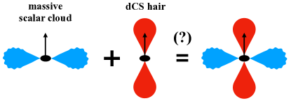
Figure 1: Sketch of a scalar field in massive dCS gravity around a rotating BH. The BH’s axis of rotation is indicated by the arrow. The blue clouds depict the QBS of a massive scalar field that is dominated by an oscillating $l=m=1$ dipole where the wavy outline indicates the QBS’s oscillations. The red clouds represent the dCS hair sourced by the Pontragin density and dominated by the $l=1,m=0$ dipole.

For this study, we have developed the Canuda-dCS code module [148] for Canuda, our open-source numerical relativity code for fundamental physics [149, 150]. Specifically, we implemented the dCS field equations for a massive scalar field in the decoupling approximation, in which the background is determined by GR and the backreaction of the scalar onto the metric is neglected.

In this paper we report a series of results to address three questions:

1. How does the nonminimal coupling to curvature affect the (equatorial) massive scalar cloud?

2. How does the mass term affect the dCS hair?

3. What is the scalar’s characteristic frequency spectrum in massive dCS gravity?

The bulk of the results are presented in Sec. IV, but let us give you a sneak preview here:

1. We find that the evolution of the massive scalar cloud in the equatorial plane (with the leading contribution being the $l=m=1$ multipole; see blue cloud in Fig. 1) appears unaffected by the nonminimal coupling to the Pontryagin density far from the BH, i.e., it is indistinguishable from its GR counterpart (within numerical error). See Sec. IV.1.

2. We find that the dCS hair sourced by the Pontryagin density grows (with the leading contribution being the $l=1,m=0$ dipole; see red cloud in Fig. 1), and it oscillates with a frequency determined by the mass. Its amplitude, suppressed by the mass, is smaller than in the massless dCS case. See Sec. IV.2.

3. We reconstruct the power spectrum of the scalar multipoles by computing the discrete Fourier transform of our data. Within the resolution allowed by our simulations and within the decoupling approximation, we observe that the characteristic frequencies of the QBSs are compatible with known results in GR. See Sec. IV.3.

Our time evolutions monitor the growth of the massive, oscillating dCS hair and suggest a new, oscillating steady-state solution as end-state. A detailed analysis of this QBS solution and its stability is subject to future work.

The paper is organized as follows: In Sec. II we present the action and field equations of massive dCS gravity, the scalar’s time evolution equations and initial conditions, and the background spacetime. In Sec. III we discuss our numerical relativity framework, introduce our open-source Canuda-dCS code  [148], and describe the series of simulations that we conducted. In Sec. IV we present our results addressing questions $1.$-$3.$ posed above. We conclude in Sec. V. Snapshots of some of our simulations are displayed in App. D, and animations of our simulations are available on our Canuda youtube channel [151].

In this paper, we use natural units $G=c=\hbar=1$ and adopt the mostly-plus signature convention for the metric, $(-,+,+,+)$.

II Setting the stage

II.1 Action and field equations

We consider dCS gravity in which a dynamical pseudoscalar field $\Theta$ is nonminimally coupled to gravity. The action is given by [85, 86]

$$S =\int d^{4}x\frac{\sqrt{-g}}{16\pi}\left[R+\frac{\alpha_{\rm CS}}{4}f(\Theta)\,^{*}RR-\frac{1}{2}(\nabla\Theta)^{2}-V(\Theta)\right]\,,$$ (1)

where $\alpha_{\rm CS}$ is a coupling constant with dimension $[\alpha_{\rm CS}]=[L]^{2}$, $V({\rm\Theta})$ is the field’s potential, and $f(\Theta)$ is a general function that couples $\Theta$ to the Pontryagin density

$$\,^{\ast}\!RR= \,{}^{\ast}\!R^{abcd}R_{bacd}=-\frac{1}{2}\tensor{\epsilon}{{}^{c}{}^{d}_{e}{}_{f}}R^{abef}R_{abcd}\,.$$ (2)

Here, $R_{abcd}$ and $\,{}^{\ast}\!R^{abcd}=\frac{1}{2}\tensor{\epsilon}{{}^{c}{}^{d}_{e}{}_{f}}R^{abef}$ are the Riemann and dual Riemann tensors associated to the metric $g_{ab}$. Note that the Pontryagin density transforms as a pseudoscalar under parity transformations, i.e., it is parity-odd. Consequently, the field $\Theta$ also transforms as a pseudoscalar field under parity transformations such that the Lagrangian in Eq. (1) is parity-even. That is, the field $\Theta$ is an axionlike particle and in the following we refer to it as “axion” or “dCS axion.”

We extend the original dCS action [86] to allow for a general coupling function $f({\rm\Theta})$ and a general potential $V({\rm\Theta})$; see Eq. (1). The function $f(\Theta)$ selects different parity-violating theories of gravity. For example, nondynamical Chern-Simons theory corresponds to $f=\rm{const}$, while the traditional dCS model corresponds to $f(\Theta)\sim\Theta$ and vanishing potential $V(\Theta)=0$ [86] .

In the present work we consider massive dCS gravity, determined by

$$f(\Theta)=\Theta\,,\quad V(\Theta)=\frac{\mu^{2}}{2}\Theta^{2}\,,$$ (3)

where $\mu$ is the mass-energy of the scalar field. We focus on fields that are light enough to form long-lived QBSs around astrophysical BHs [32, 17, 20]. We expect such a scenario when the Compton wavelength of the field is comparable to the BH’s radius. This corresponds to $2\mu M\sim 1$ in natural units or, equivalently, $\mu\simeq 10^{-10}(M_{\odot}/M)$ eV.

In the following we make our model selection given by Eq. (3) explicit, and refer to App. C for the general expressions as implemented in our Canuda-dCS code. Then, varying the action in Eq. (1) with respect to the metric and the scalar field, we obtain the field equations

$$\left(\Box-\mu^{2}\right)\Theta+\frac{\alpha_{\rm CS}}{4}\,^{\ast}\!RR=0\,,$$ (4a)

$$G_{ab}-\frac{1}{2}T^{\Theta}_{ab}+\alpha_{\rm CS}~{}\mathcal{C}_{ab}=0\,,$$ (4b)

where $G_{ab}=R_{ab}-\frac{1}{2}g_{ab}R$ is the Einstein tensor, and $T^{\Theta}_{ab}$ indicates the canonical scalar field stress tensor

$$T^{\Theta}_{ab}=\nabla_{a}\Theta\nabla_{b}\Theta-\frac{1}{2}g_{ab}\left((\nabla\Theta)^{2}+\mu^{2}\Theta^{2}\right)\,.$$ (5)

The extension of Einstein’s equations is captured by the C-tensor

$$\mathcal{C}^{ab}\equiv\mathcal{E}_{c}\,\tensor{\epsilon}{{}^{c}{}^{d}{}^{e}{}^{(}{}^{a}}\nabla_{e}\tensor{R}{{}^{b}{}^{)}_{d}}+\mathcal{F}_{cd}\,^{*}R^{d(ab)c}$$ (6)

where the auxiliary tensors $\mathcal{E}_{c}$ and $\mathcal{F}_{cd}$ are defined as

$$\mathcal{E}_{a} =\nabla_{a}\Theta\,,\quad{\textrm{and}}\quad\mathcal{F}_{ab}=\nabla_{a}\nabla_{b}\Theta\,.$$ (7)

For completeness, we also list the effective energy-momentum tensor. Using the convention $G_{ab}=\frac{1}{2}T^{\rm{eff}}_{ab}$ and comparing to Eq. (4b), we find

$$T^{\rm{eff}}_{ab}=T^{\Theta}_{ab}-2\alpha_{\rm CS}\mathcal{C}_{ab}\,,$$ (8)

where $T^{\Theta}_{ab}$ and $\mathcal{C}_{ab}$ are given in Eqs. (5) and (6).

Here, we work in the decoupling approximation, i.e., we study the evolution of the massive dCS field in a background spacetime determined by Einstein’s equations in vacuum. We apply the decoupling approximation to the field Eqs. (4), and rescale $\Theta\rightarrow(\alpha_{\rm CS}/M^{2})\,\Theta$ to obtain 

$$\Box\Theta-\mu^{2}\Theta+\frac{\hat{\alpha}M^{2}}{4}\,^{\ast}\!RR=0\,,$$ (9a)

$$G_{ab}=0\,.$$ (9b)

In Eq. (9a) we introduce the dimensionless parameter $\hat{\alpha}$ that allows us to switch the coupling to the Pontryagin density on ($\hat{\alpha}=1$) and off ($\hat{\alpha}=0$). This switch parameter enables us to compare against the evolution of a massive scalar field in GR.

II.2 Spacetime split and background metric

To conduct the numerical simulations of the scalar field, we rewrite Eqs. (9) as a time evolution problem. We obtain the 3+1 formulation by foliating the spacetime $\left(\mathcal{M},g_{ab}\right)$ into a set of spatial hypersurfaces $\left(\Sigma_{t},\gamma_{ij}\right)$ with induced metric $\gamma_{ij}$. Each hypersurface $\Sigma_{t}$ is labelled by the time parameter $t$ and the $3$-metric is given by $\gamma_{ab}=g_{ab}+n_{a}n_{b}$ where $n^{a}$ is the timelike unit vector normal to the hypersurface, $\gamma^{a}{}_{b}n^{b}=0$, with normalization $n^{a}n_{a}=-1$. Furthermore, the spatial metric defines a projection operator

$$\gamma^{a}{}_{b}= \delta^{a}{}_{b}+n^{a}n_{b}\,.$$ (10)

The line element takes the form

$$\textrm{d}s^{2}= g_{ab}\textrm{d}x^{a}\textrm{d}x^{b}$$ (11)

$$= -\left(\alpha^{2}-\beta^{k}\beta_{k}\right)\textrm{d}t^{2}+2\gamma_{ij}\beta^{i}\textrm{d}t\textrm{d}x^{j}+\gamma_{ij}\textrm{d}x^{i}\textrm{d}x^{j}\,.$$

where $\alpha$ and $\beta^{i}$ are, respectively, the lapse function and shift vector. We denote the covariant derivative and Ricci tensor associated to the 3-metric $\gamma_{ij}$ as $D_{i}$ and $R_{ij}$. The extrinsic curvature $K_{ab}$ describes how a hypersurface is embedded in the spacetime manifold and is defined as

$$K_{ab}= -\gamma^{c}{}_{a}\gamma^{d}{}_{b}\nabla_{c}n_{d}=-\frac{1}{2}\mathcal{L}_{n}\gamma_{ab}\,,$$ (12)

where $\mathcal{L}_{n}$ is the Lie derivative along $n^{a}$.

In this paper, we evolve the scalar field on a fixed, stationary background described by the Kerr metric in quasi-isotropic coordinates [153, 149], which we briefly summarize here. We start from the Kerr metric in Boyer-Lindquist (BL) coordinates $(t,r_{\rm{BL}},\theta,\phi)$,

$$\textrm{d}s^{2}= -\left(1-\frac{2Mr_{\rm{BL}}}{\Sigma}\right)\textrm{d}t^{2}-\frac{4aMr_{\rm{BL}}\sin^{2}\theta}{\Sigma}\textrm{d}t\textrm{d}\phi$$

$$+\frac{\Sigma}{\Delta}\textrm{d}r_{\rm{BL}}^{2}+\Sigma\textrm{d}\theta^{2}+\frac{\mathcal{A}}{\Sigma}\sin^{2}\theta\textrm{d}\phi^{2}$$ (13)

with

$$\Delta =(r_{\rm{BL}}-r_{\rm{BL,+}})(r_{\rm{BL}}-r_{\rm{BL,-}})$$ (14a)

$$\Sigma =r_{\rm{BL}}^{2}+a^{2}\cos^{2}\theta$$ (14b)

$$\mathcal{A} =(r_{\rm{BL}}^{2}+a^{2})^{2}-\Delta a^{2}\sin^{2}\theta$$ (14c)

$$r_{\rm{BL,\pm}} =M\pm\sqrt{M^{2}-a^{2}}\,,$$ (14d)

where $r_{\rm{BL}}$ is the BL radial coordinate, $r_{\rm{BL,\pm}}$ are the inner and outer horizons in BL coordinates, $M$ is the BH mass and $a/M$ its dimensionless spin. We introduce the quasi-isotropic radial coordinate $r\in(0,\infty)$. as [153, 149],

$$~{}r_{\rm{BL}}=r\left(1+\frac{r_{\rm{BL,+}}}{4r}\right)^{2}\,.$$ (15)

The outer horizon in these coordinates sits at $r_{+}=r_{\rm{BL,+}}/4$, while the inner horizon and the region inside are not covered.

We apply the coordinate transformation, Eq. (15), to Eq. (II.2). We write the resulting metric in the 3+1 form of Eq. (11), where the gauge functions and 3-metric are

$$\gamma_{ij}= {\textrm{Diag}}\left[\frac{(4r+r_{\rm{BL,+}})^{2}\Sigma}{16r^{3}(r_{\rm{BL}}-r_{\rm{BL,-}})},\Sigma,\frac{\mathcal{A}}{\Sigma}\sin^{2}\theta\right]\,,$$ (16a)

$$\alpha= \pm\sqrt{\frac{\Delta\Sigma}{\mathcal{A}}}\,,\quad\beta^{i}=\left(0,0,-\frac{2aMr_{\rm{BL}}}{\mathcal{A}}\right)\,.$$ (16b)

The extrinsic curvature’s nonvanishing components are

$$K_{r\phi}= \alpha\frac{aMr_{\rm{BL}}^{\prime}\sin^{2}\theta}{\Delta\Sigma^{2}}[2r_{\rm{BL}}^{2}(r_{\rm{BL}}^{2}+a^{2})+\Sigma(r_{\rm{BL}}^{2}-a^{2})]\,,$$

$$K_{\theta\phi}= -2\alpha\frac{a^{3}Mr_{\rm{BL}}\sin^{3}\theta}{\Sigma^{2}}\,,$$ (17)

where $r_{\rm{BL}}^{\prime}=\partial_{r}r_{\rm{BL}}$. We apply a final coordinate transformation from the quasi-isotropic spherical coordinates $Y^{a}=(r,\theta,\phi)$ to Cartesian coordinates $X^{i}=(x,y,z)$ via

$$x=r\cos\phi\sin\theta\,,\quad y=r\sin\phi\sin\theta\,,\quad z=r\cos\theta\,.$$ (18)

The spatial metric in Cartesian coordinates then reads

$$~{}\gamma_{ij}\textrm{d}X^{i}\textrm{d}X^{j}= \psi_{0}^{4}\left[\eta_{ij}\textrm{d}X^{i}\textrm{d}X^{j}+G(x\textrm{d}x+y\textrm{d}y+z\textrm{d}z)^{2}\right.$$

$$\left.+a^{2}H(x\textrm{d}y-y\textrm{d}x)^{2}\right]\,,$$ (19)

where $\eta_{ij}$ is the flat spatial metric and we introduced

$$\psi_{0}^{4}=\frac{\Sigma}{r^{2}}\,,\quad G=\frac{r_{\rm{BL}}}{r^{2}(r_{\rm{BL}}-r_{\rm{BL,-}})}\,,\quad H=\frac{\Sigma+2Mr_{\rm{BL}}}{r^{2}\Sigma^{2}}\,.$$ (20)

We obtain the extrinsic curvature and shift vector in Cartesian coordinates via the coordinate transformation

$$K_{ij}= J_{i}{}^{a}J_{j}{}^{b}K_{ab}\,,\quad\beta_{i}=J_{i}{}^{a}\beta_{a}\,.$$ (21)

where $J_{i}{}^{a}=\partial Y^{a}/\partial X^{i}$ is the Jacobian.

II.3 Time evolution formulation at decoupling

To derive the axion evolution equations (as a set of first order in time differential equations) we introduce the momentum of the scalar field as

$$K_{\rm\Theta}= -\mathcal{L}_{n}\Theta\,.$$ (22)

Inserting Eq. (22) into the field equation, Eq. (9a), and rewriting it in terms of the 3+1 variables, $(\gamma_{ij},K_{ij},\alpha,\beta^{i})$, we obtain the evolution equations

$$\textrm{d}_{\rm t}\Theta= -\alpha K_{\rm\Theta}\,,$$ (23a)

$$\textrm{d}_{\rm t}K_{\rm\Theta}= -\alpha D^{i}D_{i}\Theta-D^{i}\alpha D_{i}\Theta$$

$$+\alpha\left(KK_{\rm\Theta}+\mu^{2}\Theta-\frac{\hat{\alpha}M^{2}}{4}\,^{\ast}\!RR\right)\,.$$ (23b)

where $\textrm{d}_{\rm t}=\left(\partial_{t}-\mathcal{L}_{\beta}\right)$, and $\mathcal{L}_{\beta}$ is the Lie derivative along the shift vector. In the decoupling limit, the scalar is sourced by the Pontryagin density in Eq. (2), evaluated on the GR background

$$\,^{\ast}\!RR=\,^{*}W_{abcd}W^{bacd}=-16E^{ij}B_{ij}\,,$$ (24)

where ${}^{\ast}W_{abcd}=\frac{1}{2}\epsilon_{cd}{}^{ef}W_{abef}$ is the dual Weyl tensor and we introduce its gravito-electric, $E_{ij}=\gamma^{a}{}_{i}\gamma^{b}{}_{j}n^{c}n^{d}W_{acbd}$, and gravito-magnetic, $B_{ij}=\gamma^{a}{}_{i}\gamma^{b}{}_{j}n^{c}n^{d}\,{}^{\ast}W_{acbd}$, components. We compute the gravito-electric and gravito-magnetic components of the Weyl tensor in terms of the 3+1 variables, given by

$$E_{ij}= R^{\rm tf}_{ij}+\frac{1}{3}A_{ij}K-A_{i}{}^{k}A_{jk}+\frac{1}{3}\gamma_{ij}A_{kl}A^{kl}\,,$$ (25a)

$$B_{ij}= -\epsilon_{(i|}{}^{kl}D_{l}A_{|j)k}\,,$$ (25b)

where $R^{\rm tf}_{ij}$ is the trace-free part of the spatial Ricci tensor associated to $\gamma_{ij}$, $K=\gamma^{ij}K_{ij}$ is the trace of the extrinsic curvature, and $A_{ij}=K_{ij}-\frac{1}{3}\gamma_{ij}K$ is its trace-free part. The explicit 3+1 form of the scalar’s effective energy-momentum tensor in Eq. (8) is given in App. C.

We re-write the evolution equations, Eqs. (23), in terms of the Baumgarte-Shapiro-Shibata-Nakamura (BSSN) variables for the metric given by

$$W= \gamma^{-\frac{1}{6}}\,,\quad\tilde{\gamma}_{ij}=W^{2}\gamma_{ij}\,,$$ (26a)

$$K= \gamma^{ij}K_{ij}\,,\quad\tilde{A}_{ij}=W^{2}\left(K_{ij}-\frac{1}{3}\gamma_{ij}K\right)\,,$$ (26b)

$$\tilde{\Gamma}^{i}= \tilde{\gamma}^{kl}\tilde{\Gamma}^{i}{}_{kl}\,.$$ (26c)

The resulting evolution equations are given by

$$\textrm{d}_{\rm t}\Theta= -\alpha K_{\rm\Theta}\,,$$ (27a)

$$\textrm{d}_{\rm t}K_{\rm\Theta}= -W^{2}\tilde{D}^{i}\alpha\tilde{D}_{i}\Theta-\alpha\left(W^{2}\tilde{D}^{i}\tilde{D}_{i}\Theta-W\tilde{D}^{i}\Theta\tilde{D}_{i}W\right.$$

$$\left.-KK_{\rm\Theta}-\mu^{2}\Theta+\frac{\hat{\alpha}M^{2}}{4}\,^{\ast}\!RR\right)\,$$ (27b)

where we raise indices with the conformal metric $\tilde{\gamma}^{ij}$. The Pontryagin density becomes

$$\,^{\ast}\!RR= -16\tilde{\gamma}^{ia}\tilde{\gamma}^{jb}\tilde{E}_{ab}\tilde{B}_{ij}$$ (28)

where the gravito-electric and gravito-magnetic components of the Weyl tensor in BSSN variables $\tilde{E}_{ij}$ and $\tilde{B}_{ij}$ are given by Eqs. (62) in App. C.

II.4 Scalar field initial data

In our numerical simulations we perform a series of runs with different types of initial data for the scalar field. This includes a trivial field, a Gaussian type perturbation, the solution for the massless dCS axion, and the QBS solution for massive fields in GR.

Initial data 1 (ID1): Zero scalar field. The simplest initial data that we consider is the trivial one, in which we set both the scalar field and its momentum to zero,

$$\Theta(t=0)=0=K_{\Theta}(t=0)\,.$$ (29)

Although this data is not a solution of the field equation, Eq. (9a), (except for a Schwarzschild BH), it allows us to follow the formation of the massive dCS hair around a Kerr BH until it forms a steady-state configuration.

Initial data 2 (ID2): Gaussian. A second choice of initial data for the scalar field $\Theta$ is that of a Gaussian shell centered around $r_{0}$ given by

$$\Theta(t=0)=A\,\exp\left\{-\frac{(r-r_{0})^{2}}{\sigma^{2}}\right\}\Sigma_{lm}(\theta,\phi),$$ (30)

where $A$ is the amplitude, $\sigma$ is the width, and $\Sigma_{lm}$ is a superposition of spherical harmonics. In the present paper, we typically choose $\Sigma_{11}=Y_{1-1}-Y_{11}$. We also set a vanishing scalar momentum, $K_{\rm\Theta}(t=0)=0$. For our choice of angular profile, this solution is exact

$$K_{\rm\Theta}(t=0)= -\frac{1}{\alpha}\left(\partial_{t}-\beta^{a}\partial_{a}\right)\Theta|_{t=0}=\frac{\beta^{\phi}}{\alpha}\partial_{\phi}\Theta|_{t=0}=0\,,$$ (31)

as follows from the metric in Eq. (16), the definition from Eq. (22), and the profile from Eq. (30) with $\Sigma_{lm}=\Sigma_{11}$.

Initial data 3 (ID3): dCS hair. As a third choice of initial data, we implement the small-spin, small-coupling perturbative solution for the BH hair in (massless) dCS gravity [106, 154, 88]

$$\Theta= \hat{\alpha}\frac{a}{M}\left(\frac{5M^{2}}{8r_{\rm{BL}}^{2}}+\frac{5M^{3}}{4r_{\rm{BL}}^{3}}+\frac{9M^{4}}{4r_{\rm{BL}}^{4}}\right)\cos\theta$$ (32)

$$-\hat{\alpha}\frac{a^{3}}{M^{3}}\left[\left(\frac{M^{2}}{16r_{\rm{BL}}^{2}}+\frac{M^{3}}{8r_{\rm{BL}}^{3}}+\frac{3M^{4}}{20r_{\rm{BL}}^{4}}+\frac{M^{5}}{10r_{\rm{BL}}^{5}}\right)\cos\theta\right.$$

$$\left.+\left(\frac{3M^{4}}{4r_{\rm{BL}}^{4}}+\frac{3M^{5}}{r_{\rm{BL}}^{5}}+\frac{25M^{6}}{3r_{\rm{BL}}^{6}}\right)\cos^{3}\theta\right]+\mathcal{O}\left(\left(\frac{a}{M}\right)^{5}\right)\,,$$

where $a/M$ is the dimensionless BH spin and $M$ is the BH mass. We note that this solution is accurate to first-order in the dCS coupling and accurate to third-order in the spin. Similar to the construction of ID2, we can set

$$K_{\rm\Theta}(t=0)=\frac{\beta^{\phi}}{\alpha}\partial_{\phi}\Theta|_{t=0}=0\,.$$ (33)

Initial data 4 (ID4): Quasibound state. Finally, we implement initial data given by a monochromatic QBS for massive scalar fields in GR, following Ref. [32]. We take a mode ansatz for the scalar field,

$$\Theta_{lm}=\exp(-i\omega t)\exp(im\phi)\mathcal{S}_{lm}(\theta)\mathcal{R}_{lm}(r_{\rm{BL}})\,,$$ (34)

where $\omega=\bar{\omega}+\imath\bar{\nu}$ is the complex frequency, $\mathcal{S}_{lm}(\theta)$ are the $s=0$ spheroidal harmonics [155], $\mathcal{R}_{lm}(r_{\rm{BL}})$ is the radial profile, and $r_{\rm{BL}}$ is the BL radial coordinate that is related to the numerical radial coordinate via Eq. (15). We compute the spheroidal harmonics using the continued fraction method with a three-term recurrence relation and implement Eqs. (2.2) – (2.9) of Ref. [155].

To compute the radial function $\mathcal{R}_{lm}$ we implement the scheme laid out in Ref. [32]. Because we are interested in QBS solutions, we set boundary conditions that are ingoing at the horizon and vanish at infinity. This behaviour is incorporated in the ansatz for the radial function

$$\mathcal{R}_{lm}(r_{\rm{BL}}) =\Delta_{+}^{-i\eta}\Delta_{-}^{i\eta+\chi-1}e^{q\,r_{\rm{BL}}}\sum_{n=0}^{\infty}a_{n}\left(\frac{\Delta_{+}}{\Delta_{-}}\right)^{n}\,,$$ (35)

where

$$\Delta_{+} =r_{\rm{BL}}-r_{\rm{BL,+}}\,,\quad\Delta_{-}=r_{\rm{BL}}-r_{\rm{BL,-}}\,,$$ (36a)

$$\eta =\frac{2r_{\rm{BL,+}}(\omega-\omega_{\rm{c}})}{r_{\rm{BL,+}}-r_{\rm{BL,-}}}\,,\quad\chi=\frac{\mu^{2}-2\omega^{2}}{q}\,,$$ (36b)

$$q =\pm\sqrt{\mu^{2}-\omega^{2}}\,,$$ (36c)

and $\omega_{\rm{c}}=m\Omega_{\rm{H}}=m\frac{a}{2Mr_{\rm{BL,+}}}$ is the critical frequency for superradiance. The coefficients $a_{n}$ in Eq. (35) are solved for numerically by adopting Leaver’s continued fraction method [156] and using a three-term recurrence relation; see Eqs. (35) – (45) of Ref. [32].

Finally, the initial scalar field is $\Theta_{lm}(t=0)=\exp(im\phi)\mathcal{S}_{lm}(\theta)\mathcal{R}_{lm}(r_{\rm{BL}})$ with the spheroidal harmonics and radial function solved for numerically as described above. As a simplifying assumption to compute the scalar’s initial momentum, we set the initial gauge functions to $\alpha=1$, $\beta^{i}=0$, and obtain

$$K_{\rm\Theta}{}_{,lm}(t=0) =i\omega\Theta_{lm}(t=0)\,.$$ (37)

III Numerical relativity framework

In this section, we describe the numerical relativity framework and the simulations that we have performed.

III.1 Code description

To perform our numerical experiments, we employ the Einstein Toolkit [157, 158, 159], an open-source numerical relativity code for computational astrophysics, with our open-source Canuda code [150, 46, 149, 136] for fundamental physics. The Einstein Toolkit is based on the Cactus computational toolkit [160, 161], and the Carpet driver [162, 163] to provide boxes-in-boxes adaptive mesh refinement (AMR) and MPI parallelization.

Here, we focus on a stationary BH background given by the Kerr metric in quasi-isotropic coordinates as described in Sec. II.2. The metric is implemented in the KerrQuasiIsotropic thorn (as code modules in the Einstein Toolkit are called) of Canuda.

To simulate the massive dCS field, we implement the new arrangement Canuda-dCS [148]. The latter is a collection of thorns that provide the scalar field initial data and the implementation of the scalar’s time evolution equations. Since the scalar field initial data types ID1 – ID3 in Sec. II.4 are analytical, we simply assign the indicated function values in quasi-isotropic coordinates; see Eq. (15). For the QBS initial data (ID4 in Sec. II.40, we implement Leaver’s continued fraction method to solve for the spheroidal harmonics and the radial function.

We implement the scalar field evolution equations in terms of the BSSN metric variables, Eqs. (26), and solve them using the methods of lines. Spatial derivatives are realized by fourth-order finite differences, and we use a fourth-order Runge-Kutta scheme for the time integration. Fifth order Kreiss-Oliger dissipation is employed as provided by the Einstein Toolkit to reduce the high-frequency, numerical noise produced by the refinement boundaries. At the outer boundary we apply radiative boundary conditions via the NewRad thorn [164].

To analyze our data, we compute the $(l,m)$ multipoles of $\Theta$ using the Multipole thorn. In particular, the field $\Theta$ is interpolated onto spheres of fixed extraction radii $r_{\rm{ex}}$ and projected onto $s=0$ spherical harmonics $Y_{lm}(\theta,\phi)$,

$$\Theta_{lm}(t,r_{\rm{ex}})= \int\textrm{d}\Omega\,\Theta(t,r_{\rm{ex}},\theta,\phi)Y^{\ast}_{lm}(\theta,\phi)\,.$$ (38)

We visualize our numerical data with PyCactus or PostCactus [165], a set of tools for post-processing data generated with the Einstein Toolkit.

III.2 Simulations

We perform a series of simulations to study the evolution of a massive scalar field, nonminimally coupled to gravity through the Pontryagin density to address the questions posed in Sec. I. We list our simulations in Table 1, where we indicate the name of the runs, the axion’s dimensionless mass parameter $\mu M$, the dimensionless BH spin $a/M$, and the type of initial data “ID.” We also indicate the switch parameter $\hat{\alpha}$, where $\hat{\alpha}=0$ and $\hat{\alpha}=1$ refer to evolutions in GR and dCS gravity, respectively.

Run	$\mu M$	$a/M$	$\hat{\alpha}$	ID
a01_SF11_mu$00$	$0.0$	$0.1$	$1$	ID2
a01_SF11_mu$01$	$0.1$	$0.1$	$1$	ID2
a01_SF11_mu$03$	$0.3$	$0.1$	$1$	ID2
a01_SF11_mu$10$	$1.0$	$0.1$	$1$	ID2
a07_SF11_mu$00$	$0.0$	$0.7$	$1$	ID2
a07_SF11_mu$01$	$0.1$	$0.7$	$1$	ID2
a07_SF11_mu$0187$	$0.187$	$0.7$	$1$	ID2
a07_SF11_mu$10$	$1.0$	$0.7$	$1$	ID2
a099_SF11_mu$00$	$0.0$	$0.99$	$\{0,1\}$	ID2
a099_SF11_mu$01$	$0.1$	$0.99$	$1$	ID2
a099_SF0_mu$042$	$0.42$	$0.99$	$1$	ID1
a099_SF11_mu$042$	$0.42$	$0.99$	$\{0,1\}$	ID2
a099_dCSHair_SF11_mu$042$	$0.42$	$0.99$	$1$	ID2 + ID3
a099_dCSHair_mu$042$	$0.42$	$0.99$	$1$	ID3
a099_SF_QBS_mu$042$	$0.42$	$0.99$	$\{0,1\}$	ID4
a099_SF11_mu$10$	$1.0$	$0.99$	$1$	ID2

Table 1: Summary of simulations of a scalar field with dimensionless mass parameter $\mu M$ around a Kerr BH with dimensionless spin $a/M$. We set $\hat{\alpha}=1$ ($\hat{\alpha}=0$) for simulations in dCS gravity (GR). We indicate the choice of initial data, ID, as described in Sec. II.4.

In the majority of our simulations, we set $\hat{\alpha}=1$ and initialize the massive scalar field as a Gaussian, ID2 in Sec. II.4, with angular distribution $\Sigma_{lm}=\Sigma_{11}$, width $\sigma=1M$, amplitude $A=1$ and centered around $r_{0}=6M$; see Eq. (30). Note that in the absence of the coupling to the Pontryagin density, the $l=m=1$ scalar multipole is the fastest growing superradiant mode. In the majority of our simulations we set $\Theta_{10}(t=0)=0$ to follow the growth of this mode that, in the absence of the mass term, would be the leading contribution to the dCS hair.

To check the robustness of our results, we perform a set of complementary simulations with different scalar field initial data in the background of a BH with spin $a/M=0.99$. In particular, we compare our results against a scalar field initialized as a QBS in the $l=m=1$ multipole with $\mu M=0.42$, ID4 in Sec. II.4, both in GR and in dCS gravity. We also initialize the $l=1,m=0$ scalar multipole as the massless dCS hair given in Eq. (32). This choice of initial data allows us to explore the evolution of the dCS hair in the presence of a mass term.

Our simulations are performed on three-dimensional Cartesian grids with the outer boundary located at $256M$. We use the boxes-in-boxes AMR grid structure provided by Carpet [162, 163] with seven refinement levels. The level’s “radii” (half of the boxes’ lengths) are given by $\{256,128,32,6,3,1.5,0.75\}$. On the outermost domain we set the grid spacing to $\textrm{d}x=1M$, which results in a spacing of $\textrm{d}x/2^{\rm{RL}-1}=\textrm{d}x/2^{6}=1/64M$ on the innermost level that contains the BH. We set the time step to $\textrm{d}t=0.25\textrm{d}x$ on each refinement level such that the Courant-Friedrichs-Lewy condition is satisfied.

To assess the numerical error of our simulations, we perform a convergence analysis of the scalar’s $l=1,m=0$ and $l=m=1$ multipoles for Run a099_SF11_mu042 in Table 1. For this purpose, we simulate a099_SF11_mu042 with the additional coarse resolution $\textrm{d}x_{c}=1.1M$ and the high resolution $\textrm{d}x_{h}=0.9M$. The default choice for our simulations, $\textrm{d}x=1.0M$, corresponds to the medium resolution run. At intermediate times of $t\sim 500M$, we find a relative error of $\Delta\Theta_{10}/\Theta_{10,h}\lesssim 10\%$ for the $l=1,m=0$ mode and $\Delta\Theta_{11}/\Theta_{11,h}\lesssim 0.2\%$ for the $l=m=1$ mode. At late times of $t\sim 1000M$, we find a relative error of $\Delta\Theta_{10}/\Theta_{10,h}\lesssim 12\%$ for the $l=1,m=0$ mode and $\Delta\Theta_{11}/\Theta_{11,h}\lesssim 0.1\%$ for the $l=m=1$ mode. The difference of the relative numerical error for the different multipoles can be understood by the absolute value of $\Theta_{10}$ being about one order of magnitude smaller than that of $\Theta_{11}$, while $\Delta\Theta$ between the coarse and high resolutions are comparable. Details of the convergence study are presented in App. B.1 and illustrated in Fig. 18.

IV Results

In this section, we present the results of our simulations of the massive dCS field, $\Theta$, that we evolve in the background of a Kerr BH. They aid us in addressing the questions posed in the introduction, namely (i) How does the nonminimal coupling to curvature affect the (equatorial) massive scalar cloud? (ii) How does the mass term affect the dCS hair? (iii) What is the scalar’s characteristic frequency spectrum in massive dCS gravity?

We illustrate our setup in the sketch shown in Fig. 1. Here, the blue cloud represents the oscillatory, massive scalar cloud dominated by a $l=m=1$ mode, and the red cloud represents the static dCS hair dominated by a $l=1,m=0$ mode. For small spins these modes essentially decouple, as we demonstrate in App. A. Therefore, we first study the impact of the coupling to the Pontryagin density on the $l=m=1$ mode in Sec. IV.1, then we study the impact of the mass term on the $l=1,m=0$ mode in Sec. IV.2, and finally we present a spectral analysis of the massive dCS field in Sec. IV.3.

Figs. 2 and 3 give an overview of our results, where we show the time evolution of the $\Theta_{10}$ (left panels) and $\Theta_{11}$ (right panels) multipoles in massive dCS gravity. In Fig. 2 we initialize the field as a $l=m=1$ Gaussian, see Eq. (30). We consider a series of mass parameters $\mu M$ for the scalar field and three different spins $a/M=0.1$ (top), $a/M=0.7$ (middle), and $a/M=0.99$ (bottom) for the BH in the background. In Fig. 3 we initialize the scalar field as a QBS with $\mu M=0.42$, and we concentrate on a BH with dimensionless spin $a/M=0.99$. Independently of the initial data type, BH spin and mass parameter, the time evolution of the massive mode, $\Theta_{11}$, appears largely unaffected by the coupling to the Pontryagin density as is discussed in Sec. IV.1. In Sec. IV.2, we demonstrate that the mass term modifies the evolution of the dCS hair, $\Theta_{10}$. In Figs. 7 and 10 we present snapshots of the massive dCS scalar with $\mu M=0.42$ and $a/M=0.99$ in the $xy$ and the $xz$ planes, taken at $t=250M$. These are compared, respectively, against GR ($\hat{\alpha}=0$) and massless dCS gravity ($\hat{\alpha}=1$ and $\mu M=0$). In Figs. 8 and  11 we provide a close-up view on the scalar’s structure near the BH. Full 2D animations of the scalar field evolution are available on the Canuda code’s youtube channel  [151].

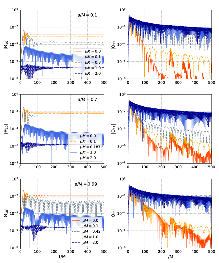
Figure 2: Evolution of the $l=1,m=0$ (left) and $l=m=1$ (right) multipoles of the massive dCS field $\Theta$, measured at $r_{\rm{ex}}=10$M, in the background of a rotating BH with dimensionless spin $a/M=0.1$ (top), $a/M=0.7$ (middle) and $a/M=0.99$ (bottom). The field is initialized as a Gaussian with $\Sigma_{lm}=\Sigma_{11}$ in Eq. (30). We vary the field’s mass parameter $\mu M$ as listed in the legends. The $l=1,m=0$ multipole (left panel) approaches the dCS solution for $\mu M=0.0$. For $\mu M\neq 0$, the dCS hair is suppressed, and for a range of small mass parameters, the dCS hair exhibits an oscillatory behaviour. The $l=m=1$ mode (right panel) exhibits the quasinormal ringdown for $\mu M=0$, intermediate or late-time massive power-law tails for small or large $\mu M$, or a QBS for intermediate $\mu M$.

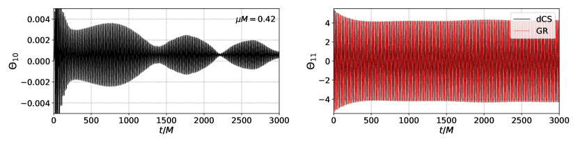
Figure 3: Same as Fig. 2 but for the field $\Theta$ initialized as the massive, $l=m=1$ QBS, ID4 in Sec. II.4 with $\mu M=0.42$ around a BH with $a/M=0.99$. We show the $l=1,m=0$ (left) and the $l=m=1$ (right) multipole, extracted at $r_{\rm{ex}}=10M$. We compare the dCS field (black solid lines) to the evolution in GR (red dashed line). The $l=m=1$ mode (right panel) remains a nearly constant-in-time QBS, and the dCS and GR case appear indistinguishable. Instead, the $l=1,m=0$ dCS hair (left panel) oscillates with a frequency induced by the massive $\Theta_{11}$ mode.

IV.1 Effect of the Pontryagin density on the evolution of a massive quasibound state

In this section we focus on the $\Theta_{11}$ multipole and investigate how its evolution is affected by the coupling to the Pontryagin density. To explore this effect, we initialize the $\Theta_{11}$ mode either as a Gaussian with $\Sigma_{11}$ in Eq. (30) or as a QBS, see Eq. (34), while we set $\Theta_{10}(t=0)=0$. The main results are shown in the right panels of Fig. 2, where we present the time evolution of $\Theta_{11}$ for a variety of mass parameters $\mu M$ and for BH spins $a/M=0.1$ (top), $a/M=0.7$ (middle), and $a/M=0.99$ (bottom). We see that the massless field (solid red lines) decays exponentially in time consistent with a quasinormal ringdown. Instead, the field with a small mass $\mu M=0.1$ (dashed-dot orange lines) exhibits a short ringdown phase followed by an oscillatory power-law tail consistent with an intermediate time massive tail [166]. For intermediate masses, $\mu M=0.187,0.3,0.42$ (dashed gray lines), the field appears to transition to a long-lived QBS, consistent with the solutions of Ref. [32] and the simulations in Ref. [39]. Finally, fields with a larger masses, $\mu M=1.0$ (solid blue) and $\mu M=2.0$ (dash-dotted dark blue), oscillate with a frequency $\bar{\omega}\sim\mu$ and decay with a universal power-law tail that is consistent with the very late-time tail of massive fields [167, 168].

This qualitative behaviour is compatible with that of massive scalar fields evolving around Kerr BHs in GR. This begs the questions: Are the decay rates for the ringdown, the QBS, and the late time tails modified by the coupling to the Pontryagin density? Does the Pontryagin density modify the scalar’s profile near the BH where the curvature is largest? To answer the first question we compare the evolution of the $l=m=1$ QBS in GR and in dCS gravity in Fig. 3 and present fits of the ringdown and tails, respectively, in Figs. 4 - 6. To address the second question, we inspect the two-dimensional snapshots in Fig. 8 showing the scalar field profile near the BH.

Let us start by analyzing the QBS. For this purpose, we initialize the field $\Theta$ as a QBS with $l=m=1$, mass parameter $\mu M=0.42$, and oscillation frequency $M\bar{\omega}=0.409$ in the background of a Kerr BH of spin $a/M=0.99$ using the solution of Ref. [32]; see ID4 in Sec. II.4. The $\Theta_{10}$ multipole is initialized as zero, but it assumes nonzero values during the evolution because it is sourced by the Pontryagin density; see left panel of Fig. 3.

We evolve two cases for this QBS and show its $l=m=1$ multipole measured at $r_{\rm{ex}}=10$M in the right panel of Fig. 3. In the first case, we set $\hat{\alpha}=0$, such that the field’s equation of motion (9a) reduces to the Klein-Gordon equation in GR (red dashed line in Fig. 3). In the second case, we set $\hat{\alpha}=1$ in Eq. (9a), such that the massive field is also sourced by the Pontryagin density (black solid line in Fig. 3). Note, that we are not attempting to follow the evolution of the superradiant instability as the timescales for massive scalars are prohibitively long for $3+1$ simulations (with the shortest e-folding timescale being $\tau\sim 10^{7}$M [32]). Instead, our goal is to compare the evolution in the presence and absence of the Pontryagin term. Both curves exhibit an oscillatory signal which, after a short transition period, remains almost constant in time. More importantly, both curves appear indistinguishable. Indeed, a quantitative analysis shows that the curves differ by $|\Theta_{11,{\rm{GR}}}-\Theta_{11,{\rm{dCS}}}|/\Theta_{11,{\rm{GR}}}\sim 4\times 10^{-15}$, consistent with round off error. In summary, in the wave-zone, the QBS of a massive dCS field around a highly spinning Kerr BH is the same as that of a massive scalar in GR, within numerical error.

We next analyze the quasinormal ringdown or massive power-law tail of massive dCS fields around a BH with dimensionless spin $a/M=0.1$ in Fig. 4, $a/M=0.7$ in Fig. 5, and $a/M=0.99$ in Fig. 6. We display the numerical data of $\Theta_{11}$ (black solid lines) and a fit to its functional behaviour (red dashed lines). In these figures, we present results for fields with $\mu M=0.0$ (left panels), $\mu M=0.1$ (middle panels) and $\mu M=1.0$ (right panels).

The massless field (left panels of Figs. 4– 6) exhibits a quasinormal ringdown pattern $\propto\exp(-\imath\,\omega t)=\exp(-\imath\bar{\omega}t)\exp(\bar{\nu}t)$ where $\bar{\omega}$ is the mode’s oscillation frequency and $\bar{\nu}$ indicates its decay (or growth) rate. For the BH with spin $a/M=0.1$ our numerical data gives $M\omega=0.29-\imath\,9.75\times 10^{-2}$, and for a BH with $a/M=0.7$ we find $M\omega=0.395-\imath\,8.88\times 10^{-2}$. Both results are in good agreement, within $4.2\%$, with frequency-domain computations in GR [169, 170, 171]. We note that the slight modulation of $\Theta_{11}$ around the BH with $a/M=0.7$, seen in the left panel of Fig. 5, is likely due the superposition with an overtone close to the fundamental mode. For the highly spinning BH with $a/M=0.99$, we find $M\omega=0.49-\imath\,3.95\times 10^{-2}$, which agrees with the frequency-domain result in GR within $7.6\%$ [170]. This is compatible with the numerical error around highly spinning BHs; see, e.g., Ref. [39] and App. B.1.

The scalar with $\mu M=0.1$, shown in the middle panels of Figs. 4– 6, exhibits a quasinormal ringdown followed by an oscillatory power-law tail. We fit the latter with the functional behaviour $\Theta_{11}\propto t^{-(l+3/2)}\sin(\mu t)=t^{-5/2}\sin(0.1t)$ which is consistent with the intermediate time massive tails in GR [166]. Here, “Intermediate time” refers to the time interval $1<t/M<1/(\mu M)^{3}=1000$. Again, we find no measurable deviation from the GR value even around the highly rotating BH.

For a larger mass, $\mu M=1.0$, shown in the right panels of Figs. 4– 6, we find an oscillating power-law decay $\propto t^{-p}\sin(\mu t)$ with $p=0.910$ for $a/M=0.1$, $p=0.920$ for $a/M=0.7$, and $p=0.925$ for $a/M=0.99$. This is within $\sim 10\%$ of the universal, very late-time power-law tail of $p=5/6$ known for massive fields in GR [168, 167, 172, 173, 174]. We note that we find comparable results for a mass parameter $\mu M=2.0$ (not displayed here).

To aid our analysis, we present 2D snapshots of the scalar field with $\mu M=0.42$ evolved around a BH with spin $a/M=0.99$ at time $t=250M$. Fig. 7 shows a color map of the scalar’s amplitude in the equatorial plane (left panel) and in the $xz$ plane (right panel) on the entire numerical domain. Fig. 8 zooms in close to the BH. The left half of each panel shows the massive scalar field in GR (i.e., with $\hat{\alpha}=0$), while the right half shows the massive field in dCS gravity (i.e., with $\hat{\alpha}=1$).

Comparing the two cases, we see that the scalar cloud’s profile in the equatorial plane is essentially unaffected by the nonminimal coupling to gravity via the Pontryagin density both in the far region (see Fig. 7) and near the BH (see Fig. 8). One is brought to similar conclusions about the far-region when considering the snapshots in the $xz$ plane: the oscillatory pattern of the nonminimally coupled massive scalar field matches that of the minimally coupled one at large distances. This pattern changes close to the BH as can be seen in the right panel of Fig. 8. Here, the spacetime curvature and, hence, the Pontryagin density is largest and it sources an axi-symmetric, dipolar scalar structure along the $z$-axis. This dipole connects smoothly to the oscillation pattern at distances larger than $\sim 1/(\mu M)^{2}$. Note, that in the absence of the mass-term this dipole would correspond to the dCS hair given in Eq. (32). We also note, that such a $l=1,m=0$ structure is absent if there is no coupling to the Pontryagin density; see left half of the right panel in Fig. 8.

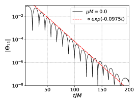
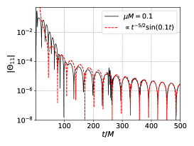
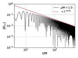
Figure 4: Evolution of the $\Theta_{11}$ mode, measured at $r_{\rm{ex}}=10$M, with $\mu M=0.0$ (left), $\mu M=0.1$ (middle), $\mu M=1.0$ (right) around a BH with spin $a/M=0.1$. We show our numerical data (solid black lines) and compare it to the analytic solutions computed in GR (dashed red lines). Left: The massless field follows a quasinormal ringdown with decay rate $M\bar{\nu}=-9.75\times 10^{-2}$. Middle: The field with $\mu M=0.1$ exhibits a short ringdown followed by an oscillating, intermediate-time power-law tail with frequency $\bar{\omega}\sim\mu$. Right: The field decays at a rate consistent with the very-late time power-law tail $\sim t^{-5/6}$.

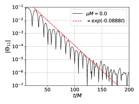
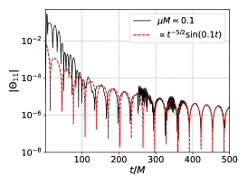
Figure 5: Same as Fig. 4 but for a BH with dimensionless spin $a/M=0.7$.

Figure 6: Same as Fig. 4 but for a BH with dimensionless spin $a/M=0.99$.

In summary, the evolution of the massive $l=m=1$ dipole around rotating BHs in dCS gravity appears consistent with that of massive fields in GR at sufficiently large distances. It only differs near the BH along the axis of rotation, where $m=0$ scalar multipoles are sourced by the Pontryagin density. We have demonstrated that this result is robust against different choices of initial data for $\Theta_{10}$ and $\Theta_{11}$, and that it holds also for highly spinning BHs. The simulations indicate that, at late times, the scalar field approaches an oscillating, quasistationary dipole configuration.

Figure 7: 2D snapshots of the massive scalar field $\Theta$ at $t=250M$. The field with $\mu M=0.42$ is evolved around a BH with $a/M=0.99$. We show the field in the equatorial plane (left panel) and in the $xz$ plane (right panel). The latter also indicates the BH’s rotation axis with a magenta arrow. We compare the evolution of a massive scalar field in GR ($\hat{\alpha}=0$, left halves) and in dCS gravity ($\hat{\alpha}=1$, right halves). At large distances, the scalars’ profiles appear almost identical.

Figure 8: Same as Fig. 7, but zoomed in near the BH. There is no visible evidence of the Pontryagin density affecting the scalar cloud in the $xy$ plane (left panel). In the $xz$ plane (right panel), however, we see that the Pontryagin density sources the $l=1,m=0$ scalar multipole, absent in GR, that exhibits the same features as the massless dCS hair near the BH and then transitions to an oscillating QBS configuration at large distances.

IV.2 Effect of the mass term on the evolution of the dynamical Chern-Simons hair

In this section we analyze how the growth and evolution of the dCS hair is affected by the mass term. Therefore, we evolve the massive dCS field around a single rotating BH according to Eqs. (27). We typically initialize $\Theta_{10}=0$ and $\Theta_{11}$ as a Gaussian or as a QBS.

In the left panels of Fig. 2 we present the time evolution of $\Theta_{10}$, measured at $r_{\rm{ex}}=10M$, for a variety of the axion’s mass parameter $\mu M$ and for BH spins $a/M=0.1$ (top), $a/M=0.7$ (middle), and $a/M=0.99$ (bottom). The massless field (solid red lines) grows over $t\sim 100$M until it reaches a constant value that corresponds to the dCS hair at this extraction radius; see Eq. (32). The hair’s final magnitude $|\Theta_{10}|$ increases with increasing BH spin, in agreement with the solutions of Ref. [109].

As the mass parameter $\mu M$ of the scalar field increases, the magnitude of the dCS hair, $\Theta_{10}$, decreases. Specifically, for small masses $\mu M=0.1$ (dashed-dotted orange lines), the dCS hair approaches a constant magnitude that is smaller than in the massless case. For intermediate masses, $\mu M\sim 0.3\ldots 0.4$ (dashed gray lines), the dCS hair reaches a smaller magnitude and, more importantly, it oscillates. The oscillation frequencies of the $\Theta_{10}$ and $\Theta_{11}$ modes are determined by the mass parameter. They are consistent with the QBS frequencies in GR [34, 32, 175], that are given by

$$\omega_{lmn}\simeq\mu\left(1-\frac{(\mu M)^{2}}{2(l+n+1)^{2}}\right)\,,$$ (39)

in the limit $\mu M\ll 1$. We refer to Sec. IV.3 for the detailed spectral analysis. This response of the $\Theta_{10}$ mode is present for both Gaussian and QBS initial data of $\Theta_{11}$; compare the left panels of Figs. 2 and 3. As the field’s mass parameter exceeds $\mu M\gtrsim 1.0$, the magnitude of $\Theta_{10}$ is reduced or entirely suppressed, as illustrated in the left panel of Fig. 2 for $\mu M=1.0,2.0$.

To understand this behaviour, we plot the late-time profile of the field $\Theta$, evolved around a BH with spin $a/M=0.99$ for different $\mu M$, along the BH’s rotation axis in Fig. 9. For a massless field (solid red line), this late-time solution is the dCS hair sourced by the Pontryagin density. For comparison we also display the $\sim 1/z^{2}$ fall-off (dash-dotted black line) found for analytical solutions in the small-spin approximation [105], and we find excellent agreement. For a massive scalar field with a small mass $\mu M=0.1$ (dashed orange line), we find that it behaves like the massless case until about $z\sim 100M$ from the BH. At larger distances from the BH the field oscillates. Both the location and the frequency of this oscillation is determined by the mass parameter. The position of this transition appears consistent with the peak of the QBS found in GR for small mass parameters given by [17, 176, 20]

$$r_{\rm{QBS,max}}\sim\frac{l(l+1)}{(\mu M)^{2}}M\,.$$ (40)

For a field with $l=1$ and $\mu M=0.1,0.42,1.0$ this corresponds to $r_{\rm{QBS,max}}\sim 200M,11.3M,2M$. We find consistent results for the dCS field with mass $\mu M=0.42$ (dotted light blue line in Fig. 9): it follows a $\sim 1/z^{2}$ fall-off close to the BH and begins to oscillate around $z\sim 10M$ where its frequency determined by $\mu M$ at larger distances. For comparison we also show the late-time profile of a field with $\mu M=0.42$ evolved in GR (solid blue line), and demonstrate that, along the z-axis, it remains several orders of magnitude smaller than its counterpart in dCS gravity. We interpret this as a further indication that the oscillation of the dCS hair is indeed induced by the mass term.

This behaviour becomes even clearer in the 2D snapshots in Figs. 10 and 11 where we display the amplitude of the scalar field at $t=250M$ on the entire numerical domain and close to the BH, respectively. Specifically, we display $\Theta$, evolved around a BH with spin $a/M=0.99$, in the equatorial plane (left panels) and the $xz$ plane (right panels). We compare the massive dCS field with $\mu M=0.42$ (right halves of each panel) against the massless dCS field (left halves of each panel). In the massless case, the initial $l=m=1$ perturbation propagates outwards so that the field vanishes in the equatorial plane (see left half of left panel) and only the $l=1$, $m=0$ dCS hair that is sourced by the Pontryagin density remains (see left half of right panel). This is to be expected because the Pontryagin density vanishes in the equatorial plane due to the axisymmetry of the background. The massive case, displayed in the right halves of Figs. 10 and 11, exhibits two distinct features: (i) it also has a dipolar structure close to the BH, but with a smaller magnitude than in the massless case (see right panel in Fig. 11), and (ii) it has an oscillatory pattern at large distances, both in the equatorial and in the $xz$ plane, due to the mass term.

Figure 9: Profile of the massive dCS field $\Theta$ with mass parameters $\mu M=0.0$ (solid red line), $\mu M=0.1$ (dashed yellow line), $\mu M=0.42$ (dotted blue line) along the rotation axis, evolved around a BH with $a/M=0.99$ at $t=500$M. For comparison, we display the expected fall-off of the dCS hair with vanishing mass (dash-dotted black line) and the profile of a scalar field with $\mu M=0.42$ in GR (solid dark blue line).

Figure 10: 2D snapshots of the dCS field $\Theta$, initialized as a $l=m=1$ Gaussian and evolved around a BH with $a/M=0.99$, at $t=250M$. We show the field in the equatorial plane (left panel) and in the $xz$ plane (right panel), where the magenta arrow indicates the BH’s rotation axis. We compare the evolution of a massless dCS field ($\mu M=0.0$, left halves) and that of a massive dCS field with $\mu M=0.42$ (right halves). Left panel: the massless field (left half) decays as the $l=m=1$ perturbation is propagating off the grid. The massive field (right half) develops an oscillating scalar cloud. Right panel: the massless field (left half) develops the dCS hair, i.e., a $l=1$, $m=0$ dipolar configuration. The massive field (right half), exhibits a suppressed dipolar configuration close to the BH that is smoothly connected to an oscillating cloud at large distances.

Figure 11: Same as Fig. 10 but zoomed in near the BH. Left panel: dCS field in the $xy$ plane. The massless field (left half) has decayed, while the field with $\mu M=0.42$ (right half) has formed an oscillating scalar cloud. Right panel: dCS field in the $xz$ plane. The massless field (left half) develops the axi-symmetricdCS hair. The massive dCS field develops a similar dipolar structure with a smaller amplitude that smoothly transitions to the oscillating cloud induced by the mass term.

For the results presented thus far, we only initialized the $l=m=1$ multipole of the field $\Theta$. Hence, our findings refer to the growth of the $l=1$, $m=0$ scalar mode. How robust are our results against different types of initial data? What would be the fate of the dCS hair if it was already present in the initial data? And, reversely, does the formation of the oscillating dCS dipole require the presence of the massive $l=m=1$ mode?

We present answers to these questions in Fig. 12, where we compare the evolution of $|\Theta_{10}|$ of a field with $\mu M=0.42$ around a BH with $a/M=0.99$ for different initial data: (i) a Gaussian shell with $\Sigma_{11}$ in Eq. (30), and $\Theta_{10}(t=0)=0$ (solid blue line), (ii) a $\Sigma_{11}$ Gaussian shell and $\Theta_{10}$ given by the dCS hair in Eq. (32) (solid pink line), (iii) $\Theta_{11}(t=0)=0$and $\Theta_{10}$ given by the dCS hair in Eq. (32) (dotted green line), and (iv) $\Theta(t=0)=0$(dash-dotted orange line). For comparison we also show the evolution of a massless field with ID2 ($\Sigma_{11}$ in Eq. (30)) and $\Theta_{10}=0$ (solid black line). The initially hairy, massive field (solid pink line) decays and approaches the magnitude of the initially hairless, massive field (solid blue line). That is, the transformation of the time-independent hairy solution in massless dCS gravity into an oscillating dipole with a lower amplitude appears to be a robust feature in massive dCS gravity and independent of the initial data choice for the $l=1,m=0$ multipole. Similarly, we do not find any difference in the evolution of $\Theta_{10}$ for different initial data of the $l=m=1$ mode. Compare, e.g., the field initialized as zero (dash-dotted orange line) with the one initialized as a $\Sigma_{11}$ Gaussian shell (solid blue line).

In summary, we investigated the effect of a mass term on the formation and evolution of the dCS hair. We have identified a new, oscillating hairy solution in massive dCS gravity consisting of an axi-symmetric dipole near the BH that smoothly transitions to an oscillating dipole at large distances. This transition and the oscillation frequency are determined by the field’s mass parameter. We verified that the formation of an oscillating dipole in massive dCS gravity is a robust feature independent of the initial data.

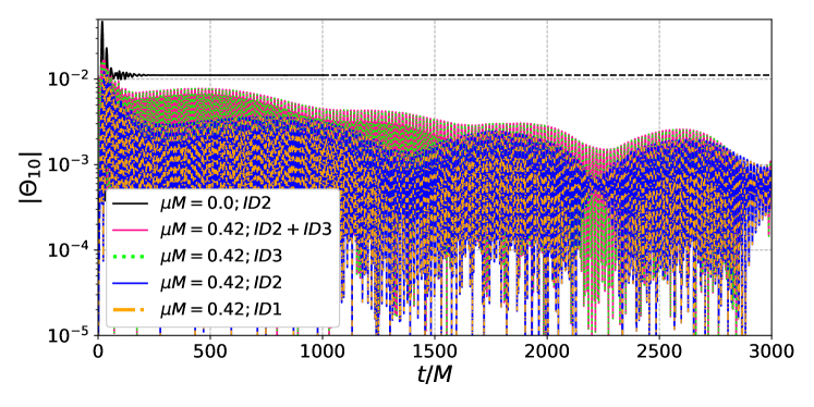
Figure 12: Evolution of the $l=1,m=0$ mode of a field with $\mu M=0.42$ evolving in the background of a BH with $a/M=0.99$ in dCS gravity ($\hat{\alpha}~{}=1$). The field is initialized as an $l=m=1$ Gaussian, ID2 with $\Sigma_{11}$ in Eq. (30) (solid blue line), or as an $l=m=1$ Gaussian plus the dCS hair, ID2+ID3 (solid pink). We compare the former with a simulation where the field is initially zero, ID1, (orange dash-dotted line) and the latter with a simulation where the field is initialized as the dCS hair, ID3, indicating $\Theta_{11}=0$ (dotted green). We find that the dCS, $\Theta_{10}$, multipole does not differ between these two comparisons, indicating that our results for the growth and evolution of $\Theta_{10}$ are independent of our choice of initial data for the massive, $\Theta_{11}$, multipole. As an additional comparison, we show the evolution of a massless field with $l=m=1$ Gaussian initial data (solid black line). We ran the massless simulation until $t=1000$M and indicate its extrapolated value (dashed black line).

IV.3 Characteristic spectra in massive dCS gravity

In this section we determine the frequency spectra of the $l=1,m=0,1$ multipoles of the dCS axion. To do so, we perform a spectral analysis of our data.

First, we obtain the time series data of the scalar field’s multipoles, $\Theta_{lm}(t,r_{\rm{ex}})$, by interpolating the field $\Theta$ onto spheres of constant extraction radii $r_{\rm{ex}}$ and projecting it onto $s=0$ spherical harmonics. We then apply a window function (typically, a Blackman-Harris window [177]) to the time series data to mitigate the effects of the initial transient, and compute the Fourier amplitude

$$\tilde{\Theta}_{lm}(\omega_{i})=\frac{1}{N}\sum_{j=0}^{N-1}\Theta_{lm}(t_{j})e^{-i\omega_{i}t_{j}}\,,$$ (41)

via a Fast Fourier Transform algorithm. Finally, we compute the power spectrum, $P_{lm}(\omega)=|\tilde{\Theta}_{lm}(\omega)|^{2}$, of the $(l,\,m)$-mode. A monochromatic signal, $\Theta_{lm}\sim\exp\left(-i\bar{\omega}t+\bar{\nu}t\right)$, with characteristic frequency $\bar{\omega}$ and growth or decay rate $\bar{\nu}$, corresponds to a power spectrum consisting of a peak described by a three-parameter Lorentzian (or Breit-Wigner) function

$$\Lambda(\omega;\bar{I},\bar{\omega},\bar{\nu})=\bar{I}\frac{\bar{\nu}^{2}}{\left((\omega-\bar{\omega})^{2}+\bar{\nu}^{2}\right)}\,.$$ (42)

The peak height is set by $\bar{I}$, while its position and width are determined by $\bar{\omega}$ and $\bar{\nu}$, respectively.

Ideally, we would like the time series extracted from our numerical simulations to be monochromatic signals with characteristic frequency $\bar{\omega}=\omega_{lmn}$, where $l$ and $m$ are the harmonic mode indices and $n$ is the overtone number. In practise, however, the extracted signals are projected only into $(lm)$ multipoles, so they still are a superposition of the fundamental ($n=0$) and overtone modes. Depending on their relative amplitude, the superposition of fundamental and overtone modes can give rise to strong modulations of the signal and beating patterns [39]. To overcome this complication we fix the extraction radius $r_{\rm{ex}}$ to a location where the overtone mode nearly vanishes. In Fig. 13 we present the profiles of the fundamental and first overtone modes of the initial scalar field, determined by a QBS with $l=m=1$ and mass parameter $\mu M=0.42$ around a BH with spin $a/M=0.99$. In this case, the overtone mode has a node at $r_{\rm{ex}}\simeq 20$M. Thus, the signal at this location is dominated by the fundamental mode and, hence, nearly monochromatic. Therefore, we choose the waveform extracted at $r_{\rm{ex}}=20$M for the spectral analysis. To measure the first overtone frequencies we additionally extract data at $r_{\rm{ex}}\simeq 50M$, where the fundamental mode is subdominant; c.f. Fig. 13.

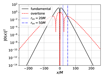
Figure 13: Initial profiles of massive scalar field $\Theta$ along the x-axis with mass $\mu M=0.42$ evolving in the background of a BH with spin $a/M=0.99$ in dCS gravity ($\hat{\alpha}=1$). We initialize the scalar field as a QBS, ID4 in Sec. II.4, with fundamental frequency $M\bar{\omega}=0.409$ (solid black) and overtone frequency $M\bar{\omega}=0.415$ (dashed red). For the spectal analysis, we extract the multipoles $\Theta_{10}$ and $\Theta_{11}$ at $r_{\rm{ex}}=20$M (dotted blue) and $r_{\rm{ex}}=50$M (dash-dotted blue).

We measure the three parameters, $(\bar{I},\bar{\omega},\bar{\nu})$, via a nonlinear regression using Eq. (42) as fitting function. This method produces reliable estimates, within $0.5\%$, of the characteristic frequency, $\omega_{lmn}$, but is greatly limited in correctly measuring the growth rate. In particular, for long-lived modes which grow or decay on timescales larger than what can be evolved in $3+1$ simulations (with reasonable computational resources), the width of the peaks is dominated by windowing effects and insufficient frequency resolution. Longer time series and different techniques, such as those employed in [38, 178] are required for more accurate estimates of the growth rates.

We present the results of the spectral analysis in Figs. 14, 15 and 16. We concentrate on the simulations with parameters $a/M=0.99$ and $\mu M=0.42$. We compute the spectra for the simulations with Gaussian initial data with $\Sigma_{lm}=\Sigma_{11}$ (ID2 in Sec. II.4), and for QBS initial data (ID4 in Sec. II.4) shown in Fig. 13.

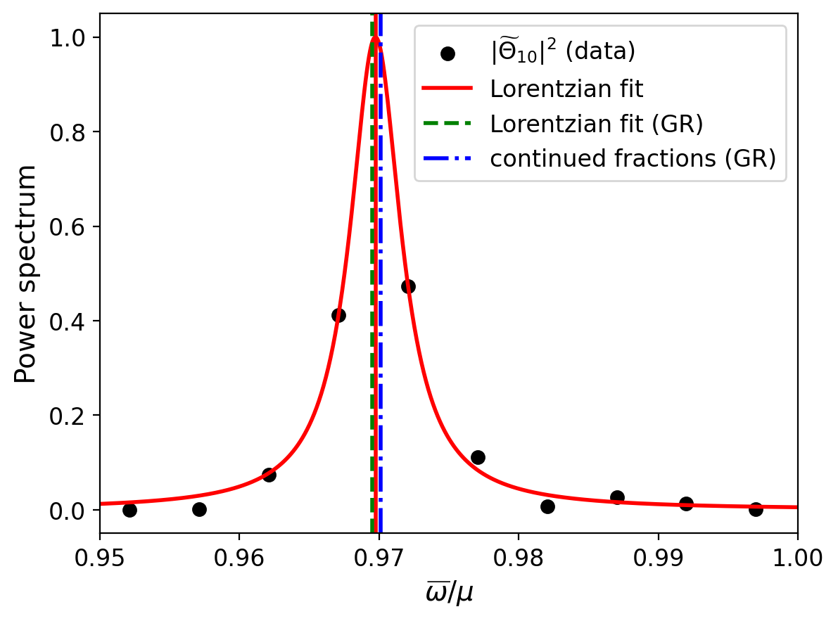
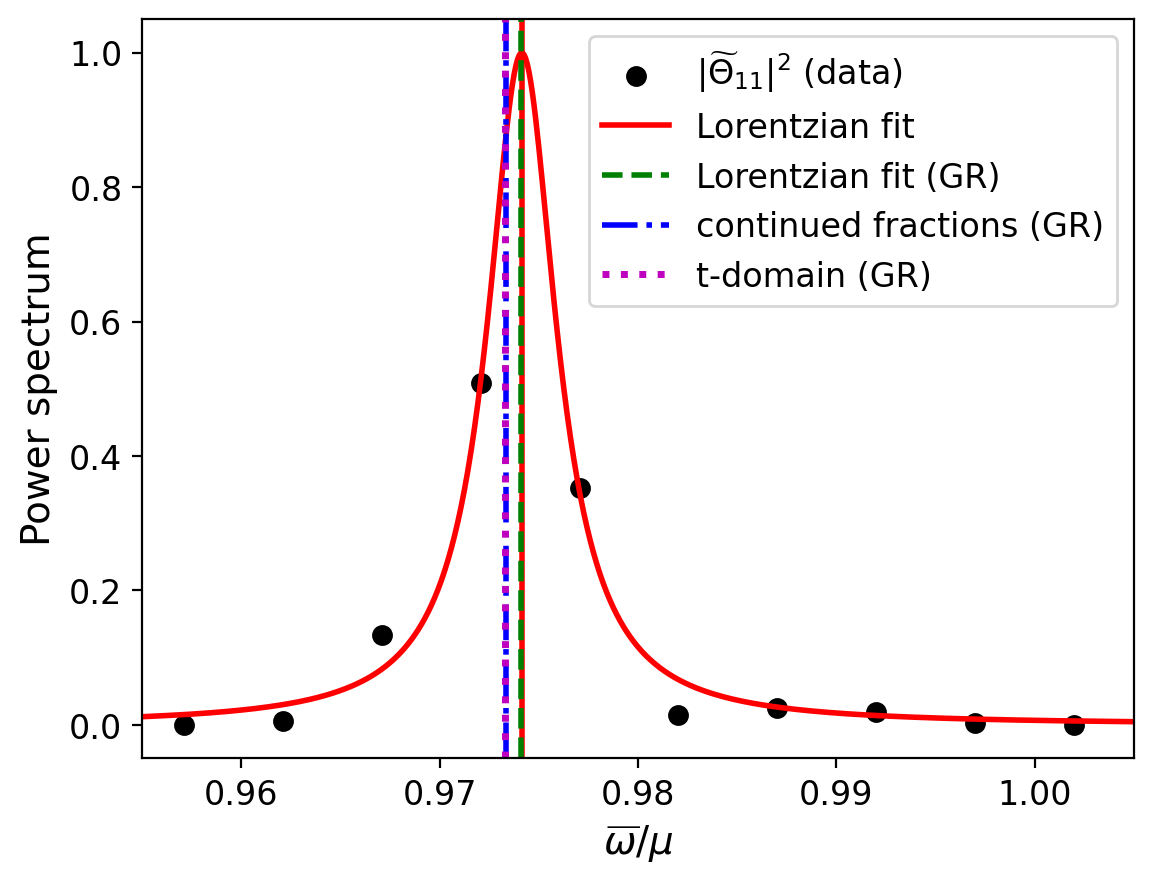
Figure 14: Power spectra reconstructed from simulations with Gaussian initial data (ID2 in Sec. II.4) and parameters $a/M=0.99$, $\mu M=0.42$, normalized by the maximum value. We indicate the numerical data (black dots), extracted at $r_{\rm{ex}}=20M$, and the Lorentzian fit to our data points (solid red line) obtained in massive dCS gravity. For comparison we also show the peak of a Lorentzian fit for the equivalent GR simulation (dashed green line) and the frequency obtained with the continued fraction method in GR [32] (dot-dashed blue line). Top panel: data and fits for the $(l,\,m,\,n)=(1,0,0)$ multipole. The fit of the data gives a peak frequency of $\bar{\omega}/\mu=0.970\pm 0.005$. Bottom panel: data and fits for the $(l,\,m,\,n)=(1,1,0)$ multipole. The fit of the data gives a peak frequency of $\bar{\omega}/\mu=0.974\pm 0.005$.

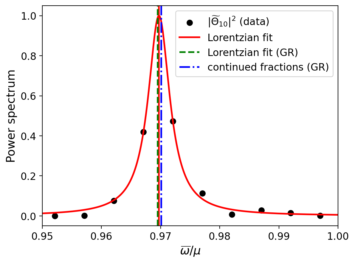
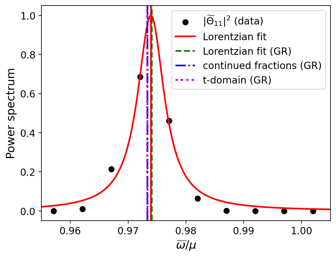
Figure 15: Same as Fig. 14 but for QBS initial data (ID4 in Sec. II.4) Top panel: data and fits for the $(l,\,m,\,n)=(1,0,0)$ multipole, and the frequency estimated from the fit is $\bar{\omega}/\mu=0.969\pm 0.005$. Bottom panel: data and fits for the $(l,\,m,\,n)=(1,1,0)$ multipole, and the frequency estimated from the fit is $\bar{\omega}/\mu=0.974\pm 0.005$.

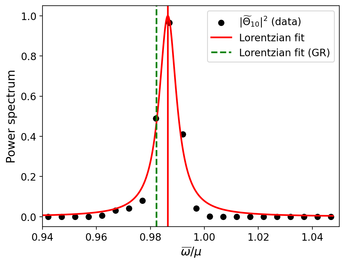
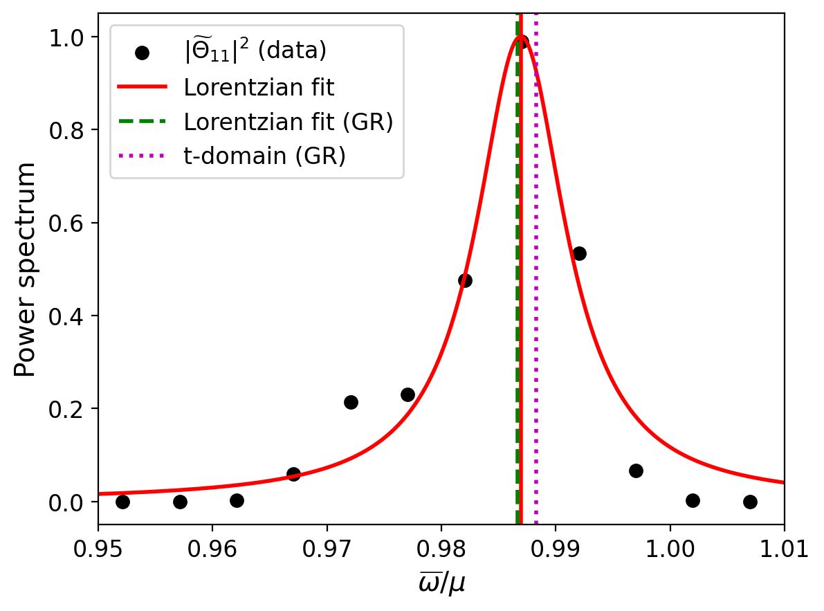
Figure 16: Same as Fig. 14 but for data extracted at $r_{\rm{ex}}=50M$, where the first overtone dominates over the fundamental $l=1$ mode. Top panel: data and fits for the $(l,\,m,\,n)=(1,0,1)$ multipole, and the frequency estimated from the fit is $\bar{\omega}/\mu=0.986\pm 0.005$. Bottom panel: data and fits for the $(l,\,m,\,n)=(1,1,1)$ multipole, and the frequency estimated from the fit is $\bar{\omega}/\mu=0.987\pm 0.005$. The power spectrum also contains the fundamental mode (see shoulder to the left of the fitted peak), but it is subdominant with respect to the $n=1$ overtone.

Fig. 14 presents the power spectra of the $l=1,m=0,n=0$ (left panel) and of the $l=m=1,n=0$ (right panel) multipoles for the simulation with Gaussian initial data, extracted at $r_{\rm{ex}}=20$M, after an evolution time of $t=3000$M. We measure the characteristic frequency of the $l=1,m=0,n=0$ mode to be $\bar{\omega}/\mu\simeq 0.970\pm 0.005$, and that of the $l=m=1,n=0$ mode to be $\bar{\omega}/\mu\simeq 0.974\pm 0.005$. We took the frequency resolution of our discrete Fourier series as a conservative estimator of the uncertainty; see App. B.2 for a detailed discussion.

We compare these estimates, obtained from the peak in the Lorentzian fit (solid red line), against the QBS frequency of a massive scalar field in GR. We obtain the latter in three different ways: (i) by fitting the data from a 3+1 simulation in which we turn off the dCS coupling, $\hat{\alpha}=0$, (dashed green line); (ii) by computing the frequency via the continued fraction method [32] (dot-dashed blue line); (iii) by fitting data from an effective, 1+1 evolution in the time domain [38] for the $l=m=1$ mode (right panels; purple dotted line). For both harmonic modes, we see no statistical evidence of a deviation from the characteristic frequencies of a minimally-coupled massive scalar field around a Kerr BH (i.e. $\hat{\alpha}=0$). This conclusion is robust against different initial data: we obtain compatible frequency measurements for QBS initial data, as can be see from Fig. 15.

We also extracted signals at $r_{\rm{ex}}=50M$, where the $n=1$ overtone becomes larger than the fundamental mode $n=0$. In Fig. 16 we show the peaks corresponding to modes $\left(l,m,n\right)=\left(1,0,1\right)$ and $\left(l,m,n\right)=\left(1,1,1\right)$, respectively. Concerning the scalar’s $l=1,m=0$ multipole, we observe a larger discrepancy with respect to the reference measure with $\hat{\alpha}=0$ that is, nonetheless, compatible with a statistical fluctuation. We find that results are overall consistent with GR, within $0.5\%$.

To summarize, we observe that the spectrum of characteristic oscillations of the massive dCS field is determined by the mass of the field. Thus, it appears indistinguishable from the QBS spectrum of a massive scalar field around a Kerr BH in GR at sufficiently large distances. This conclusion is consistent with the results of Macedo [144] for QBSs of a massive dCS field around nonrotating BHs. Because the 3+1 time domain approach does not allow for sufficiently long evolutions (at a resonable computational cost) to accurately measure to growth or decay rate of the scalar modes, we postpone the computation of this quantity in massive dCS gravity to future work using different techniques.

V Summary and conclusions

In this paper we study the phenomenology of a scalar field in massive dCS gravity, and its evolution around rotating BHs. This line of research broadens our understanding on how BH observations may be used to probe for physics beyond the standard model.

Here, we focus on “new physics” in the shape of fundamental scalar fields that can leave potentially observable footprints in the phenomenology of BHs. In particular, working in the decoupling approximation we find new, oscillating scalar configurations around rotating BHs that may give rise to new BH solutions if the backreaction of the scalar onto the metric is taken into account. Our results have a twofold interpretation: On the one hand, we may interpret the scalar field as new solutions to dCS modified gravity if a mass-term is generated by nonperturbative effects. On the other hand, we may interpret the scalar field as an axionlike particle – a popular dark matter candidate – sensitive to parity violation in the gravity sector. Thus, our results aid ongoing efforts to devise new observational tests of gravity or probes for ultralight particles that pose a class of dark matter models.

This project has been guided by three questions stated in the introduction, Sec. I, and we use the same structure to summarize our results here.

Massive scalar fields can form QBSs, or scalar clouds, around rotating BHs in GR that are predominantly determined by the $\Theta_{11}$ multipole. How does the nonminimal coupling to curvature affect such a massive scalar cloud? To address this question, we analyze the evolution of the $\Theta_{11}$ mode in massive dCS gravity for a range of mass parameters and BH spins. We observe that the QBS frequencies and, when excited, their massive power-law tails are consistent with those of massive scalar fields in GR. In addition, we compare the structure of the scalar cloud in the equatorial plane in massive dCS gravity against that found in GR. We observe no difference between the two, so we conclude that, to leading order, the coupling to the Pontryagin density has essentially no effect on the $l=m=1$ QBS. Thus, ultralight scalars representing, e.g., wavelike dark matter candidates appear insensitive to this type of parity-violating corrections to GR far from BHs. This may come as no surprise because the Pontryagin density primarily sources the $l=1,m=0$ dipole of the dCS axion.

This leads us to the second question: How does the mass term affect the dCS hair? To address this question we compare the evolution of the $\Theta_{10}$ mode in massless and in massive dCS gravity. In both cases, the Pontryagin density causes the formation of a (quasi)stationary scalar dipole close to the BH, that is absent in GR. We observe that the mass term suppresses the amplitude of the dCS hair. What is the origin of this suppression? We can exclude mode mixing between the $l=1,m=0$ and $l=m=1$ multipoles because of the symmetries of the background spacetime. In particular, modes with different azimuthal numbers $m$ decouple around the Kerr metric. It is also not due to the Pontryagin density, which inherits the axisymmetry of the background spacetime and only sources $m=0$ multipoles. Instead, we interpret the reduction of the axion’s amplitude as a Yukawa suppression due to the field’s mass.

We also observe that the mass term imprints an oscillatory pattern on the dCS hair, $\Theta_{10}$, far away from the BH as illustrated in Fig. 17. The transition from the quasistationary to an oscillating configuration occurs at $r/M\sim(\mu M)^{-2}$. The oscillation frequency of the massive dCS hair is determined by its mass parameter. Consequently, BH hair in dCS gravity would be sensitive to the presence of a mass term in the field’s potential.

Figure 17: Updated sketch (see Fig. 1) of the oscillating massive dCS hair sourced by a rotating BH. The blue clouds correspond to the QBSs in the equatorial plane and $(r/M)_{max}\sim(\mu M)^{-2}$ indicates their maximum. The red gradient along the axis of rotation indicates the oscillatory pattern of the axion that is due to the formation of a QBS peaking roughly at $r\simeq r_{max}$.

This leads us to the last question: What is the scalar’s characteristic frequency spectrum in massive dCS gravity? We analyze the frequency spectrum of the $l=1,m=0$ and the $l=m=1$ scalar multipoles in massive dCS gravity. We find that both are determined essentially by the scalar’s mass parameter.

In conclusion, we find that rotating BHs in massive dCS gravity give rise to new configurations of the dCS axion that connects an axi-symmetric dipole close to the BH with an oscillating axion “cloud” at large distances. We sketch this new configuration in Fig. 17.

Based on our results, we speculate that massive dCS gravity admits new BH solutions with an oscillating steady-state axion hair at the onset of superradiance, similar to new hairy solutions in GR [54]. Such a study would require to solve the massive dCS equations in full or perturbatively to higher order in the metric, and it is beyond the scope of the present paper.

Furthermore, while we observe the onset of massive QBSs in dCS gravity, they appear to evolve on similar timescales as scalar QBSs in GR. This makes numerical simulations in $3+1$ dimensions not well suited to conduct a detailed analysis of their evolution. Thus, we leave the hunt for superradiant instabilities in massive dCS gravity to future work using different techniques.

In conclusion, this work is the first in a series to explore the properties of BHs in the presence of axionlike particles, representing a large class of dark matter candidates, when parity is violated in the gravity sector.

Appendix A Harmonic decomposition of the Pontryagin density

In this appendix we complement our numerical results by seeking analytic insight into the effects of the nonminimal coupling to gravity onto the $(lm)$ multipoles of the massive dCS field. Therefore, we project the Pontryagin density (that sources the dCS field) onto a basis of spherical harmonic functions, $Y_{lm}(\theta,\phi)$. Working in BL coordinates, $(t,r_{\rm{BL}},\theta,\phi)$, the projection is given by

$$\,^{\ast}\!RR= \sum_{l,m}\mathcal{P}_{lm}(r_{\rm{BL}})Y_{lm}(\theta,\phi)\,,$$ (43)

$$\mathcal{P}_{lm}:= \int Y^{*}_{lm}(\theta,\phi)(\,^{\ast}\!RR)d(\cos\theta)d\phi\,,$$ (44)

where the spherical harmonics are normalized such that

$$\int Y^{*}_{lm}(\theta,\phi)Y_{kn}(\theta,\phi)d(\cos\theta)d\phi=\delta_{lk}\delta_{mn}\,.$$ (45)

In the current project, we concentrate on Kerr BHs as our background spacetime. Therefore, we focus on writing the Pontryagin density as a superposition of spherical harmonics evaluated on a Kerr background. In BL coordinates, the Kerr metric is given by Eq. (II.2) and the Pontryagin density reads

$$\,^{\ast}\!RR= 96M^{2}\frac{3r_{\rm{BL}}^{5}a\cos\theta-10r_{\rm{BL}}^{3}a^{3}\cos^{3}\theta+3r_{\rm{BL}}a^{5}\cos^{5}\theta}{\Sigma^{6}}\,,$$ (46)

where the metric function $\Sigma$ is given in Eq. (14). Note, that the Pontryagin density inherits the axisymmetry of the background spacetime and, therefore, it has no dependence on the azimuthal angle $\phi$. Consequently, the only nonvanishing spherical harmonic components, $\mathcal{P}_{lm}$, are those with $m=0$. Moreover, the parity symmetry properties of the Pontryagin density imply that it is composed of a combination of odd $l$ modes. Taking the above considerations into account, we can decompose the Pontryagin density as

$$\,^{\ast}\!RR= \sum_{j=0}^{\infty}p_{j}(r_{\rm{BL}})Y_{(2j+1)0}(\theta,\phi)\,,$$ (47)

with the projection coefficients

$$p_{j}:= 2\pi\int_{-1}^{+1}Y^{*}_{(2j+1),0}(\,^{\ast}\!RR)d(\cos\theta)\,.$$ (48)

As a result, one can conclude that the nonminimal coupling to the Pontryagin density behaves as a source term only for the scalar field multipoles with $m=0$ and odd $l$, and it does not introduce any new mode-mixing at the level of the scalar field equation.

Appendix B Error estimates

In this appendix we quantify the discretization error of our numerical simulations through a convergence analysis and the statistical error of the frequency estimates.

B.1 Convergence tests

To assess the numerical discretization error, we perform a convergence analysis of the run a099_SF11_mu042 in Table 1. This run is representative of the most demanding setups as it evolves a scalar field with mass parameter $\mu M=0.42$ in the background of a Kerr BH with spin $a/M=0.99$. The grid setup is identical to the simulations outlined in Sec. III.2, but we vary the grid spacing $\textrm{d}x_{h}/M=0.9$ (high resolution), $\textrm{d}x_{m}/M=1.0$ (medium resolution; standard choice for our simulations) and $\textrm{d}x_{l}/M=1.1$ (low resolution); see Table 2. In Table 2 we also list the resolution $h=\textrm{d}x/2^{6}$ on the innermost refinement level that encompasses the BH.

We compare the $l=1,m=0$ and $l=m=1$ multipoles of the massive dCS scalar extracted at $r_{\rm{ex}}=10M$ for the high, medium, and low resolution runs. We observe that all runs perfectly align, i.e., they are consistent across the different resolutions.

In Fig. 18 we show the convergence plot for the $l=1,m=0$ (left) and $l=m=1$ (right) multipoles of the massive dCS field. Specifically, we show the difference between the low and medium resolution waveform (solid black line), and the medium and high resolution run (dashed red line). The latter difference has been rescaled by the factor $Q_{3}=1.221$ indicating third order convergence. This is consistent with our numerical code that employs a fourth order finite difference and time integration scheme, supplemented with second order interpolation at refinement boundaries.

From the convergence analysis we can now estimate the numerical error. In particular, for the $l=1,m=0$ multipole we find $\Delta\Theta_{10}/\Theta_{10,h}\lesssim 12\%$ at late times $t\sim 1,000M$. For the $l=m=1$ multipole we find $\Delta\Theta_{11}/\Theta_{11,h}\lesssim 0.15\%$ at late times $t\sim 1,000M$.

Run	$\textrm{d}x/M$	$h/M$
a099_SF11_mu042_low	$1.1$	$1.719\times 10^{-2}$
a099_SF11_mu042_med	$1.0$	$1.563\times 10^{-2}$
a099_SF11_mu042_high	$0.9$	$1.406\times 10^{-2}$

Table 2: List of runs for the convergence tests evolving the massive dCS field with $\mu M=0.42$ around a BH with spin $a/M=0.99$. The field initially has a Gaussian profile with $\Sigma_{11}$ (ID2). We denote the resolution $\textrm{d}x/M$ on the outermost refinement level and the resolution $h=\textrm{d}x/2^{n-1}$ (with $n=7$) on the innermost refinement level.

Figure 18: Convergence plot of the $l=1,m=0$ (left) and $l=m=1$ (right) multipoles of the massive dCS field (with $\mu M=0.42$ around a BH with $a/M=0.99$). We compare the difference between the low and medium resolution run (solid black line), and the medium and high resolution run (dashed red line). The latter is rescaled by the factor $Q_{3}=1.221$ indicating third order convergence.

B.2 Frequency error estimate

To obtain the frequency estimates we perform a Fourier transformation of the numerical time series data that lasts for about $T\sim 3\times 10^{3}M$ and has a finite resolution. This gives rise to an error due to the frequency resolution that we estimate to $\sigma_{\hat{\omega}}=\Delta\hat{\omega}=\Delta\omega/\mu=2\pi/(T\mu)\simeq 0.005$ (or equivalently, $\sim 0.5\%$).

Additionally, we estimate the statistical error. Therefore, we perform a more sophisticated analysis by propagating the numerical error of the time series data through the Discrete Fourier Transform and the Breit-Wigner fitting procedure. To estimate the uncertainty in the extracted multipole $\Theta_{lm}(t;r=r_{\rm ext})$ we use the conservative estimator given by the maximum amplitude error (excluding the initial transient) taken from the convergence tests, $\sigma_{\Theta}={\rm max}\{\Delta\Theta_{lm}\}\lesssim 3\times 10^{-3}$; see Appendix B.1. Taken this conservative error in the multipole amplitude, assuming that it remains approximately constant in time and treating it as uncorrelated, the propogated error in the frequency power spectrum is given by

$$\sigma_{\rm\tilde{P}}=\frac{2\sqrt{\tilde{P}}}{\sqrt{N}}\sigma_{\Theta}\,.$$ (49)

Applying a nonlinear least square regression algorithm yields the statistical error on the fitted frequency. It is $\sigma_{\hat{\omega}}\simeq 2\times 10^{-4}$ ($0.02\%$) for the $l=m=1$ multipole frequency, and $\sigma_{\hat{\omega}}\simeq 4\times 10^{-4}$ ($0.04\%$) for the $l=1$, $m=0$ multipole. Taking both contributions together, we estimate the error in the frequency to be $\sigma_{\hat{\omega}}\lesssim 5.4\times 10^{-3}$.

Appendix C General dCS gravity at decoupling

For completeness, we derive the equations of motion and the evolution equations (at decoupling) of dCS gravity with a general coupling function $f(\Theta)$ between the dCS axion and the Pontryagin density. We vary the action, given in Eq. (1), with respect to the metric and the pseudoscalar field and obtain

$$\Box\Theta-V^{\prime}({\rm\Theta})+\frac{\alpha_{\rm CS}}{4}f^{\prime}({\rm\Theta})\,^{\ast}\!RR=0\,,$$ (50a)

$$G_{ab}-\frac{1}{2}T^{\Theta}_{ab}+\alpha_{\rm CS}~{}\mathcal{C}_{ab}=0\,,$$ (50b)

where $G_{ab}=R_{ab}-\frac{1}{2}g_{ab}R$ is the Einstein tensor, and $T^{\Theta}_{ab}$ is the canonical scalar field energy-momentum tensor

$$T^{\Theta}_{ab}=\nabla_{a}\Theta\nabla_{b}\Theta-g_{ab}\left(\frac{1}{2}(\nabla\Theta)^{2}+V({\rm\Theta})\right)\,.$$ (51)

The C-tensor captures the modification of Einstein’s equations and it is given by

$$\mathcal{C}^{ab}\equiv\mathcal{E}_{c}\,\tensor{\epsilon}{{}^{c}{}^{d}{}^{e}{}^{(}{}^{a}}\nabla_{e}\tensor{R}{{}^{b}{}^{)}_{d}}+\mathcal{F}_{cd}\,^{*}R^{d(ab)c}$$ (52)

where the auxiliary tensors $\mathcal{E}_{a}$ and $\mathcal{F}_{ab}$ are defined as

$$\mathcal{E}_{a}\equiv f^{\prime}({\rm\Theta})\nabla_{a}\Theta\,,$$ (53a)

$$\mathcal{F}_{ab}\equiv f^{\prime}({\rm\Theta})\nabla_{a}\nabla_{b}\Theta+f^{\prime\prime}({\rm\Theta})\nabla_{a}\Theta\nabla_{b}\Theta\,.$$ (53b)

As described in Sec. II.1, we work in the decoupling approximation around vacuum GR. That is, we study the evolution of the massive dCS field in a background spacetime that is determined by Einstein’s equations in vacuum. With these assumptions the Ricci tensor and its derivative vanish, $R_{ab}=0=\nabla^{e}R_{ab}$. Consequently the first term in Eq. (52) vanishes. Then we can write the C-tensor in terms of the dual Weyl tensor as,

$$\mathcal{C}^{ab}_{\text{vac;GR}}=\mathcal{F}_{cd}\,^{*}W^{d(ab)c}\,.$$ (54)

Following the same steps as in Section II.1, we apply the decoupling approximation to the field equations (50), rescale $\Theta\rightarrow(\alpha_{\rm CS}/M^{2})\Theta$ and perform the $3+1$ decomposition to find

$$\textrm{d}_{\rm t}\Theta= -\alpha K_{\rm\Theta}\,$$ (55a)

$$\textrm{d}_{t}K_{\rm\Theta}= -\alpha D^{i}D_{i}\Theta-D^{i}\alpha D_{i}\Theta$$ (55b)

$$+\alpha\left(KK_{\rm\Theta}+V^{\prime}(\Theta)-\frac{\hat{\alpha}M^{2}}{4}f^{\prime}({\rm\Theta})\,^{\ast}\!RR\right)\,$$

where $\textrm{d}_{\rm t}=\left(\partial_{t}-\mathcal{L}_{\beta}\right)$ with $\mathcal{L}_{\beta}$ being the Lie derivative along the shift vector, and we introduce the dimensionless parameter $\hat{\alpha}$ that allows us to switch the coupling to the Pontryagin density on ($\hat{\alpha}=1$) and off ($\hat{\alpha}=0$). This enables us to compare against the evolution of a massive scalar field in GR.

In the decoupling limit, the Pontryagin density is evaluated on the GR background. It is convenient to write the Pontryagin density in terms of the gravito-electric, $E_{ij}$, and gravito-magnetic, $B_{ij}$, components of the Weyl tensor given by Eqs. (25a) and (25b). Then, the Pontryagin density is

$$\,{}^{\ast}\!RR=\,^{*}W_{abcd}W^{bacd}=-16E^{ij}B_{ij}\,.$$ (56)

To estimate the effect that the dCS field and its nonminimal coupling would have onto the metric, if back-reacted onto the spacetime, we introduce the effective energy-momentum tensor

$$T^{\rm eff}_{ab}:=T^{\rm\Theta}_{ab}-2\hat{\alpha}M^{2}\mathcal{C}^{\textrm{vac;GR}}_{ab}\,.$$ (57)

In $3+1$ form, the energy-momentum tensor can be decomposed into the energy density, $\rho^{\rm eff}:=n^{a}n^{b}T_{ab}^{\rm eff}$, the energy flux, $j_{i}^{\rm eff}:=-\gamma_{i}^{a}n^{b}T_{ab}^{\rm eff}$, and the spatial stress tensor, $S^{\rm eff}_{ij}:=\gamma_{i}^{a}\gamma_{j}^{b}T_{ab}^{\rm eff}$. They are given by

$$\rho^{\rm eff}= \frac{1}{2}\left(K_{\Theta}^{2}+2V({\rm\Theta})+D_{i}\Theta D^{i}\Theta\right)+2\hat{\alpha}M^{2}\left(B^{ij}\mathcal{F}_{ij}\right)\,,$$ (58a)

$$j_{i}^{\rm eff}= K_{\Theta}D_{i}\Theta+2\hat{\alpha}M^{2}(B_{ij}\mathcal{F}^{j}-\epsilon_{ijk}E^{jl}\mathcal{F}_{l}{}^{k})\,,$$ (58b)

$$S_{ij}^{\rm eff}= D_{i}\Theta D_{j}\Theta+\frac{1}{2}\gamma_{ij}(K_{\Theta}^{2}-D_{k}\Theta D^{k}\Theta-2V({\rm\Theta}))$$

$$+2\hat{\alpha}M^{2}\left(2\epsilon_{(i|kl}E_{|j)}{}^{l}\mathcal{F}^{k}-2B_{(i}{}^{k}\mathcal{F}_{j)k}+\gamma_{ij}B^{kl}\mathcal{F}_{kl}\right.$$

$$\left.+B_{ij}(\mathcal{F}_{nn}+{\rm tr}\mathcal{F})\right)\,.$$ (58c)

Here, we introduced the decomposition of the auxiliary tensor as $\mathcal{F}_{nn}=\mathcal{F}_{ab}n^{a}n^{b}$, $\mathcal{F}_{i}=-\gamma^{a}{}_{i}n^{b}\mathcal{F}_{ab}$ and $\mathcal{F}_{ij}=\gamma^{a}{}_{i}\gamma^{b}{}_{j}\mathcal{F}_{ab}$, and its trace ${\rm tr}\mathcal{F}=\gamma^{ij}\mathcal{F}_{ij}$. They are explicitly given by

$$\mathcal{F}_{nn}= \left(D_{k}D^{k}\Theta-KK_{\Theta}-V^{\prime}({\rm\Theta})\right)f^{\prime}({\rm\Theta})$$

$$+\frac{\hat{\alpha}M^{2}}{4}\,^{\ast}\!RRf^{\prime}({\rm\Theta})^{2}+K_{\Theta}^{2}f^{\prime\prime}({\rm\Theta})\,,$$ (59a)

$$\mathcal{F}_{i}= (D_{i}K_{\Theta}-K_{ij}D^{j}\Theta)f^{\prime}({\rm\Theta})+K_{\Theta}D_{i}f^{\prime\prime}({\rm\Theta})\,,$$ (59b)

$$\mathcal{F}_{ij}= (D_{i}D_{j}\Theta-K_{ij}K_{\Theta})f^{\prime}({\rm\Theta})+D_{i}\Theta D_{j}\Theta f^{\prime\prime}({\rm\Theta})\,.$$ (59c)

In the expression for $\mathcal{F}_{nn}$ we substituted the time derivate of $K_{\rm\Theta}$ with its evolution equation, Eq. (55b).

For completeness, we also provide the BSSN formulation of the dCS scalar’s evolution equation and the energy density, flux and stress tensor to be used in an implementation of the general dCS equations. In fact, these are the equations implemented in Canuda-dCS. The BSSN variables are given in Eqs. (26). Note that, in the following, we introduce the tilde over variables to indicate that they are expressed in terms of the BSSN variables. The evolution equations, Eqs. (55), become

$$\textrm{d}_{\rm t}\Theta= -\alpha K_{\rm\Theta}\,,$$ (60a)

$$\textrm{d}_{\rm t}K_{\rm\Theta}= -W^{2}\tilde{D}^{i}\alpha\tilde{D}_{i}\Theta-\alpha\left(W^{2}\tilde{D}^{i}\tilde{D}_{i}\Theta-W\tilde{D}^{i}\Theta\tilde{D}_{i}W\right.$$

$$\left.-KK_{\rm\Theta}-V^{\prime}({\rm\Theta})+\frac{\hat{\alpha}M^{2}}{4}\,^{\ast}\!RRf^{\prime}({\rm\Theta})\right)\,,$$ (60b)

and indices are raised with the conformal metric $\tilde{\gamma}_{ij}$. In BSSN variables, the Pontryagin density $\,{}^{\ast}\!RR$ is given by

$$\,{}^{\ast}\!RR= -16\tilde{\gamma}^{ia}\tilde{\gamma}^{jb}\tilde{E}_{ab}\tilde{B}_{ij}$$ (61)

with

$$\tilde{E}_{ij}= W^{2}E_{ij}$$ (62a)

$$= W^{2}R^{\rm tf}_{ij}+\frac{1}{3}\tilde{A}_{ij}K-\tilde{A}_{i}{}^{k}\tilde{A}_{jk}+\frac{1}{3}\tilde{\gamma}_{ij}\tilde{A}_{kl}\tilde{A}^{kl}\,,$$

$$\tilde{B}_{ij}= W^{2}B_{ij}$$ (62b)

$$= -W\tilde{\epsilon}_{(i|}{}^{kl}\tilde{D}_{l}\tilde{A}_{|j)k}-\tilde{\epsilon}_{(i|}{}^{kl}\tilde{A}_{|j)l}\tilde{D}_{k}W\,.$$

Note that we insert the BSSN variables into our expressions for $B_{ij}$ and $E_{ij}$, and then rescale them by $W^{2}$ for convenience.

Similarly, we substitute the BSSN variables into the energy density, flux and spatial stress tensor (58) to find

$$\rho^{\rm eff}= \frac{1}{2}\left(K_{\Theta}^{2}+2V({\rm\Theta})+W^{2}(\tilde{D}_{i}\Theta)(\tilde{D}^{i}\Theta)\right)$$

$$+2\hat{\alpha}M^{2}(\tilde{B}^{ij}\mathcal{\tilde{F}}_{ij})\,,$$ (63a)

$$j_{i}^{\rm eff}= K_{\Theta}\tilde{D}_{i}\Theta+2\hat{\alpha}M^{2}\left(\tilde{B}_{ij}{\tilde{\mathcal{F}}^{j}}-\frac{1}{W}\tilde{\epsilon}_{ijk}\tilde{E}^{jl}\mathcal{\tilde{F}}_{l}{}^{k}\right)\,,$$ (63b)

$$S_{ij}^{\rm eff}= \tilde{D}_{i}\Theta\tilde{D}_{j}\Theta+\frac{1}{2W^{2}}\tilde{\gamma}_{ij}(K_{\Theta}^{2}-W^{2}\tilde{D}_{k}\Theta\tilde{D}^{k}\Theta-2V({\rm\Theta}))$$

$$+\frac{2\hat{\alpha}M^{2}}{W^{2}}\left(2W\tilde{\epsilon}_{(i|kl}\tilde{E}_{|j)}{}^{l}{\tilde{\mathcal{F}}^{k}}-2\tilde{B}_{(i}{}^{k}\mathcal{\tilde{F}}_{j)k}\right.$$

$$\left.+\tilde{\gamma}_{ij}\tilde{B}^{kl}\mathcal{\tilde{F}}_{kl}+\tilde{B}_{ij}(\mathcal{F}_{nn}+{\rm tr}\mathcal{F})\right)\,.$$ (63c)

The auxiliary tensors become

$$\mathcal{F}_{nn}= f^{\prime}({\rm\Theta})\Bigl{(}-KK_{\Theta}+W^{2}\tilde{D}_{k}\tilde{D}^{k}\Theta-W\tilde{D}_{k}\Theta\tilde{D}^{k}W$$

$$-V^{\prime}({\rm\Theta})\Bigr{)}+\frac{\hat{\alpha}M^{2}}{4}\,^{\ast}\!RRf^{\prime}({\rm\Theta})^{2}+{K_{\Theta}}^{2}f^{\prime\prime}({\rm\Theta})\,,$$ (64a)

$$\mathcal{F}_{i}= (\tilde{D}_{i}K_{\Theta})f^{\prime}({\rm\Theta})-(\tilde{A}_{ij}+\frac{1}{3}K\tilde{\gamma}_{ij})(\tilde{D}^{j}\Theta)f^{\prime}({\rm\Theta})$$

$$+K_{\Theta}(\tilde{D}_{i}\Theta)f^{\prime\prime}({\rm\Theta})\,,$$ (64b)

$$\mathcal{\tilde{F}}_{ij}= W^{2}\mathcal{F}_{ij}$$

$$= -(\tilde{A}_{ij}+\frac{1}{3}K\tilde{\gamma}_{ij})K_{\Theta}f^{\prime}({\rm\Theta})+W^{2}(D_{i}D_{j}\Theta)f^{\prime}({\rm\Theta})$$

$$+W^{2}(\tilde{D}_{i}\Theta)(\tilde{D}_{j}\Theta)f^{\prime\prime}({\rm\Theta})\,,$$ (64c)

where we have rescaled $\mathcal{F}_{ij}$ by $W^{2}$ for convenience and introduced the rescaled quantity $\mathcal{F}^{i}=W^{2}\tilde{\mathcal{F}}^{i}$ . Finally, the trace of the spatial projection is given by ${\rm tr}\mathcal{F}=\gamma^{ij}\mathcal{F}_{ij}=\tilde{\gamma}^{ij}\mathcal{\tilde{F}}_{ij}$ and

$$D_{i}D_{j}\Theta = \frac{\tilde{D}_{k}\Theta}{W}\left({\tilde{\gamma}^{k}}_{i}(\tilde{D}_{j}W)+{\tilde{\gamma}^{k}}_{j}(\tilde{D}_{i}W)-\tilde{\gamma}_{ij}(\tilde{D}^{k}W)\right)$$ (65)

$$+\tilde{D}_{i}\tilde{D}_{j}\Theta\,.$$

Appendix D Snapshots of numerical simulations

In this section we present 2D snapshots of our simulations to depict the growth of the scalar field around a BH with spin $a/M=0.99$ at times $t/M=\{0,100,200\}$; see Figs. 19,  20, 21 and  22. These snapshots are complementary to those shown in Sec. IV (namely Figs. 7, 8, 10, 11) that displayed the late-time evolution of the field. In each figure we present a set of frames with subpanels. The frames on the left-hand side show the amplitude of the scalar in the equatorial (i.e., x-y) plane while the frames on the right-hand side correspond to the x-z plane (along the rotation axis).

In Figs. 19 and 20, we present the snapshots of a massive scalar field with $\mu M=0.42$ evolving around a BH with spin $a/M=0.99$ to demonstrate how the initial configuration slowly grows into the oscillating scalar cloud presented in Fig. 7. The frames are in the order described above. The left panel of each frame corresponds to a massive scalar field minimally coupled to gravity, i.e., in GR. The right panel of each frame depicts the massive dCS scalar. At large scales, one can hardly observe any difference between the two simulations. On the other hand, the close-up in Fig. 20 shows how an axis-symmetric dipole forms early on in massive dCS. The growth of this dipole is absent in GR and qualitatively resembles the dipolar scalar hair that BHs grow in massless dCS. Thus, we conclude that the dipole configuration is due to the nonminimal coupling between the massive scalar and gravity via the Pontryagin density. The latter sources the axis-symmetric scalar modes close to the BH, where the curvature is strongest.

In Figs. 21 and  22, we compare snapshots of a massless (left panels in each frame) and a massive (right panels in each frame) dCS field. In the massless case, we observe how the initial Gaussian perturbation with an $l=m=1$ profile propagates outwards while a static, axi-symmetric dipole hair is formed. In the massive case, instead, the mass term traps scalar multipoles with $\bar{\omega}\lesssim\mu$ in the vicinity of the BH, and thus induces the formation of an oscillating scalar cloud that connects smoothly to the inner dipole.

The full animations made with these snapshots can be found at [151].

Figure 19: GR vs massive dCS. Snapshots of massive scalar field $\Theta$ with $\mu M=0.42$ coupled to a BH with $a/M=0.99$ in the $xy$ plane (left) and $xz$ plane (right) where z is the axis of rotation.

Figure 20: GR vs massive dCS  – closeup. Snapshots of massive scalar field $\Theta$ with $\mu M=0.42$ coupled to a BH with $a/M=0.99$ in the $xy$ plane (left) and $xz$ plane (right) where z is the axis of rotation.

Figure 21: dCS vs massive dCS. Snapshots of massive scalar field $\Theta$ with $\mu M=0.42$ coupled to a BH with $a/M=0.99$ in the $xy$ plane (left) and $xz$ plane (right) where z is the axis of rotation.

Figure 22: dCS vs massive dCS  – closeup. Snapshots of massive scalar field $\Theta$ with $\mu M=0.42$ coupled to a BH with $a/M=0.99$ in the $xy$ plane (left) and $xz$ plane (right) where z is the axis of rotation.

References

- Israel [1967] W. Israel, Phys. Rev. 164, 1776 (1967).
- Israel [1968] W. Israel, Commun. Math. Phys. 8, 245 (1968).
- Carter [1971] B. Carter, Phys. Rev. Lett. 26, 331 (1971).
- Wald [1971] R. M. Wald, Phys. Rev. Lett. 26, 1653 (1971).
- Robinson [1975] D. C. Robinson, Phys. Rev. Lett. 34, 905 (1975).
- Bekenstein [1972a] J. D. Bekenstein, Phys. Rev. D 5, 1239 (1972a).
- Bekenstein [1972b] J. D. Bekenstein, Phys. Rev. D 5, 2403 (1972b).
- Pena and Sudarsky [1997] I. Pena and D. Sudarsky, Class. Quant. Grav. 14, 3131 (1997).
- Sotiriou and Faraoni [2012] T. P. Sotiriou and V. Faraoni, Phys. Rev. Lett. 108, 081103 (2012), arXiv:1109.6324 [gr-qc] .
- Akiyama et al. [2019] K. Akiyama et al. (Event Horizon Telescope), Astrophys. J. Lett. 875, L1 (2019), arXiv:1906.11238 [astro-ph.GA] .
- Akiyama et al. [2022a] K. Akiyama et al. (Event Horizon Telescope), Astrophys. J. Lett. 930, L12 (2022a).
- Akiyama et al. [2022b] K. Akiyama et al. (Event Horizon Telescope), Astrophys. J. Lett. 930, L17 (2022b).
- Abbott et al. [2016] B. P. Abbott et al. (LIGO Scientific, Virgo), Phys. Rev. Lett. 116, 061102 (2016), arXiv:1602.03837 [gr-qc] .
- Abbott et al. [2021a] R. Abbott et al. (LIGO Scientific, VIRGO, KAGRA), GWTC-3: Compact Binary Coalescences Observed by LIGO and Virgo During the Second Part of the Third Observing Run (2021a), arXiv:2111.03606 [gr-qc] .
- Abbott et al. [2021b] R. Abbott et al. (LIGO Scientific, VIRGO, KAGRA), Tests of General Relativity with GWTC-3 (2021b), arXiv:2112.06861 [gr-qc] .
- Bambi et al. [2017] C. Bambi, A. Cardenas-Avendano, T. Dauser, J. A. Garcia, and S. Nampalliwar, Astrophys. J. 842, 76 (2017), arXiv:1607.00596 [gr-qc] .
- Arvanitaki and Dubovsky [2011] A. Arvanitaki and S. Dubovsky, Phys. Rev. D 83, 044026 (2011), arXiv:1004.3558 [hep-th] .
- Kodama and Yoshino [2012] H. Kodama and H. Yoshino, Int. J. Mod. Phys. Conf. Ser. 7, 84 (2012), arXiv:1108.1365 [hep-th] .
- Brito et al. [2015a] R. Brito, V. Cardoso, and P. Pani, Class. Quant. Grav. 32, 134001 (2015a), arXiv:1411.0686 [gr-qc] .
- Brito et al. [2015b] R. Brito, V. Cardoso, and P. Pani, Lect. Notes Phys. 906, pp.1 (2015b), arXiv:1501.06570 [gr-qc] .
- Hui et al. [2017] L. Hui, J. P. Ostriker, S. Tremaine, and E. Witten, Phys. Rev. D 95, 043541 (2017), arXiv:1610.08297 [astro-ph.CO] .
- Arvanitaki et al. [2017] A. Arvanitaki, M. Baryakhtar, S. Dimopoulos, S. Dubovsky, and R. Lasenby, Phys. Rev. D 95, 043001 (2017), arXiv:1604.03958 [hep-ph] .
- Yunes and Siemens [2013] N. Yunes and X. Siemens, Living Rev. Rel. 16, 9 (2013), arXiv:1304.3473 [gr-qc] .
- Berti et al. [2015] E. Berti et al., Class. Quant. Grav. 32, 243001 (2015), arXiv:1501.07274 [gr-qc] .
- Sotiriou [2015] T. P. Sotiriou, Class. Quant. Grav. 32, 214002 (2015), arXiv:1505.00248 [gr-qc] .
- Barack et al. [2019] L. Barack et al., Class. Quant. Grav. 36, 143001 (2019), arXiv:1806.05195 [gr-qc] .
- Sathyaprakash et al. [2019] B. S. Sathyaprakash et al., Extreme Gravity and Fundamental Physics (2019), arXiv:1903.09221 [astro-ph.HE] .
- Barausse et al. [2020] E. Barausse et al., Gen. Rel. Grav. 52, 81 (2020), arXiv:2001.09793 [gr-qc] .
- Kalogera et al. [2021] V. Kalogera et al., The Next Generation Global Gravitational Wave Observatory: The Science Book (2021), arXiv:2111.06990 [gr-qc] .
- Doneva et al. [2022] D. D. Doneva, F. M. Ramazanoğlu, H. O. Silva, T. P. Sotiriou, and S. S. Yazadjiev, Scalarization (2022), arXiv:2211.01766 [gr-qc] .
- Arun et al. [2022] K. G. Arun et al. (LISA), Living Rev. Rel. 25, 4 (2022), arXiv:2205.01597 [gr-qc] .
- Dolan [2007] S. R. Dolan, Phys. Rev. D 76, 084001 (2007), arXiv:0705.2880 [gr-qc] .
- Damour et al. [1976] T. Damour, N. Deruelle, and R. Ruffini, Lett. Nuovo Cim. 15, 257 (1976).
- Detweiler [1980] S. L. Detweiler, Phys. Rev. D 22, 2323 (1980).
- Zouros and Eardley [1979] T. J. M. Zouros and D. M. Eardley, Annals Phys. 118, 139 (1979).
- Press and Teukolsky [1972] W. H. Press and S. A. Teukolsky, Nature 238, 211 (1972).
- Cardoso et al. [2004] V. Cardoso, O. J. C. Dias, J. P. S. Lemos, and S. Yoshida, Phys. Rev. D 70, 044039 (2004), [Erratum: Phys.Rev.D 70, 049903 (2004)], arXiv:hep-th/0404096 .
- Dolan [2013] S. R. Dolan, Phys. Rev. D 87, 124026 (2013), arXiv:1212.1477 [gr-qc] .
- Witek et al. [2013] H. Witek, V. Cardoso, A. Ishibashi, and U. Sperhake, Phys. Rev. D 87, 043513 (2013), arXiv:1212.0551 [gr-qc] .
- Yoshino and Kodama [2012] H. Yoshino and H. Kodama, Prog. Theor. Phys. 128, 153 (2012), arXiv:1203.5070 [gr-qc] .
- Shlapentokh-Rothman [2014] Y. Shlapentokh-Rothman, Commun. Math. Phys. 329, 859 (2014), arXiv:1302.3448 [gr-qc] .
- Hui et al. [2023] L. Hui, Y. T. A. Law, L. Santoni, G. Sun, G. M. Tomaselli, and E. Trincherini, Phys. Rev. D 107, 104018 (2023), arXiv:2208.06408 [gr-qc] .
- Branco et al. [2023] N. P. Branco, R. Z. Ferreira, and J. a. G. Rosa, JCAP 04, 003, arXiv:2301.01780 [hep-ph] .
- Barranco et al. [2011] J. Barranco, A. Bernal, J. C. Degollado, A. Diez-Tejedor, M. Megevand, M. Alcubierre, D. Nunez, and O. Sarbach, Phys. Rev. D 84, 083008 (2011), arXiv:1108.0931 [gr-qc] .
- Barranco et al. [2012] J. Barranco, A. Bernal, J. C. Degollado, A. Diez-Tejedor, M. Megevand, M. Alcubierre, D. Nunez, and O. Sarbach, Phys. Rev. Lett. 109, 081102 (2012), arXiv:1207.2153 [gr-qc] .
- Okawa et al. [2014] H. Okawa, H. Witek, and V. Cardoso, Phys. Rev. D 89, 104032 (2014), arXiv:1401.1548 [gr-qc] .
- Sanchis-Gual et al. [2016] N. Sanchis-Gual, J. C. Degollado, P. Izquierdo, J. A. Font, and P. J. Montero, Phys. Rev. D 94, 043004 (2016), arXiv:1606.05146 [gr-qc] .
- Clough et al. [2019] K. Clough, P. G. Ferreira, and M. Lagos, Phys. Rev. D 100, 063014 (2019), arXiv:1904.12783 [gr-qc] .
- Hui et al. [2019] L. Hui, D. Kabat, X. Li, L. Santoni, and S. S. C. Wong, JCAP 06, 038, arXiv:1904.12803 [gr-qc] .
- Bamber et al. [2021] J. Bamber, K. Clough, P. G. Ferreira, L. Hui, and M. Lagos, Phys. Rev. D 103, 044059 (2021), arXiv:2011.07870 [gr-qc] .
- Traykova et al. [2021] D. Traykova, K. Clough, T. Helfer, E. Berti, P. G. Ferreira, and L. Hui, Phys. Rev. D 104, 103014 (2021), arXiv:2106.08280 [gr-qc] .
- Cardoso et al. [2011] V. Cardoso, S. Chakrabarti, P. Pani, E. Berti, and L. Gualtieri, Phys. Rev. Lett. 107, 241101 (2011), arXiv:1109.6021 [gr-qc] .
- Hod [2013a] S. Hod, Eur. Phys. J. C 73, 2378 (2013a), arXiv:1311.5298 [gr-qc] .
- Herdeiro and Radu [2014] C. A. R. Herdeiro and E. Radu, Phys. Rev. Lett. 112, 221101 (2014), arXiv:1403.2757 [gr-qc] .
- Benone et al. [2014] C. L. Benone, L. C. B. Crispino, C. Herdeiro, and E. Radu, Phys. Rev. D 90, 104024 (2014), arXiv:1409.1593 [gr-qc] .
- Herdeiro and Radu [2015a] C. Herdeiro and E. Radu, Class. Quant. Grav. 32, 144001 (2015a), arXiv:1501.04319 [gr-qc] .
- Chodosh and Shlapentokh-Rothman [2017] O. Chodosh and Y. Shlapentokh-Rothman, Commun. Math. Phys. 356, 1155 (2017), arXiv:1510.08025 [gr-qc] .
- Degollado and Herdeiro [2014] J. C. Degollado and C. A. R. Herdeiro, Phys. Rev. D 90, 065019 (2014), arXiv:1408.2589 [gr-qc] .
- Brito et al. [2017a] R. Brito, S. Ghosh, E. Barausse, E. Berti, V. Cardoso, I. Dvorkin, A. Klein, and P. Pani, Phys. Rev. Lett. 119, 131101 (2017a), arXiv:1706.05097 [gr-qc] .
- Brito et al. [2017b] R. Brito, S. Ghosh, E. Barausse, E. Berti, V. Cardoso, I. Dvorkin, A. Klein, and P. Pani, Phys. Rev. D 96, 064050 (2017b), arXiv:1706.06311 [gr-qc] .
- Ficarra et al. [2019] G. Ficarra, P. Pani, and H. Witek, Phys. Rev. D 99, 104019 (2019), arXiv:1812.02758 [gr-qc] .
- Cunha et al. [2015] P. V. P. Cunha, C. A. R. Herdeiro, E. Radu, and H. F. Runarsson, Phys. Rev. Lett. 115, 211102 (2015), arXiv:1509.00021 [gr-qc] .
- Cunha et al. [2019] P. V. P. Cunha, C. A. R. Herdeiro, and E. Radu, Universe 5, 220 (2019), arXiv:1909.08039 [gr-qc] .
- Creci et al. [2020] G. Creci, S. Vandoren, and H. Witek, Phys. Rev. D 101, 124051 (2020), arXiv:2004.05178 [gr-qc] .
- Roy et al. [2022] R. Roy, S. Vagnozzi, and L. Visinelli, Phys. Rev. D 105, 083002 (2022), arXiv:2112.06932 [astro-ph.HE] .
- Berti et al. [2019] E. Berti, R. Brito, C. F. B. Macedo, G. Raposo, and J. L. Rosa, Phys. Rev. D 99, 104039 (2019), arXiv:1904.03131 [gr-qc] .
- Zhang and Yang [2020] J. Zhang and H. Yang, Phys. Rev. D 101, 043020 (2020), arXiv:1907.13582 [gr-qc] .
- Ikeda et al. [2021] T. Ikeda, L. Bernard, V. Cardoso, and M. Zilhão, Phys. Rev. D 103, 024020 (2021), arXiv:2010.00008 [gr-qc] .
- Bamber et al. [2023] J. Bamber, J. C. Aurrekoetxea, K. Clough, and P. G. Ferreira, Phys. Rev. D 107, 024035 (2023), arXiv:2210.09254 [gr-qc] .
- Choudhary et al. [2021] S. Choudhary, N. Sanchis-Gual, A. Gupta, J. C. Degollado, S. Bose, and J. A. Font, Phys. Rev. D 103, 044032 (2021), arXiv:2010.00935 [gr-qc] .
- Hannuksela et al. [2019] O. A. Hannuksela, K. W. K. Wong, R. Brito, E. Berti, and T. G. F. Li, Nature Astron. 3, 447 (2019), arXiv:1804.09659 [astro-ph.HE] .
- Baumann et al. [2019a] D. Baumann, H. S. Chia, and R. A. Porto, Phys. Rev. D 99, 044001 (2019a), arXiv:1804.03208 [gr-qc] .
- Baumann et al. [2020] D. Baumann, H. S. Chia, R. A. Porto, and J. Stout, Phys. Rev. D 101, 083019 (2020), arXiv:1912.04932 [gr-qc] .
- Barsanti et al. [2022] S. Barsanti, A. Maselli, T. P. Sotiriou, and L. Gualtieri, Detecting massive scalar fields with Extreme Mass-Ratio Inspirals (2022), arXiv:2212.03888 [gr-qc] .
- Takahashi et al. [2023] T. Takahashi, H. Omiya, and T. Tanaka, Evolution of binary systems accompanying axion clouds in extreme mass ratio inspirals (2023), arXiv:2301.13213 [gr-qc] .
- Blas et al. [2017] D. Blas, D. L. Nacir, and S. Sibiryakov, Phys. Rev. Lett. 118, 261102 (2017), arXiv:1612.06789 [hep-ph] .
- Blas et al. [2020] D. Blas, D. López Nacir, and S. Sibiryakov, Phys. Rev. D 101, 063016 (2020), arXiv:1910.08544 [gr-qc] .
- Herdeiro and Radu [2015b] C. A. R. Herdeiro and E. Radu, Int. J. Mod. Phys. D 24, 1542014 (2015b), arXiv:1504.08209 [gr-qc] .
- Blázquez-Salcedo et al. [2016] J. L. Blázquez-Salcedo et al., IAU Symp. 324, 265 (2016), arXiv:1610.09214 [gr-qc] .
- Silva et al. [2018] H. O. Silva, J. Sakstein, L. Gualtieri, T. P. Sotiriou, and E. Berti, Phys. Rev. Lett. 120, 131104 (2018), arXiv:1711.02080 [gr-qc] .
- Doneva and Yazadjiev [2018] D. D. Doneva and S. S. Yazadjiev, Phys. Rev. Lett. 120, 131103 (2018), arXiv:1711.01187 [gr-qc] .
- Dima et al. [2020] A. Dima, E. Barausse, N. Franchini, and T. P. Sotiriou, Phys. Rev. Lett. 125, 231101 (2020), arXiv:2006.03095 [gr-qc] .
- Hegade K R et al. [2022a] A. Hegade K R, E. R. Most, J. Noronha, H. Witek, and N. Yunes, Phys. Rev. D 105, 064041 (2022a), arXiv:2201.05178 [gr-qc] .
- Kanti et al. [1996] P. Kanti, N. E. Mavromatos, J. Rizos, K. Tamvakis, and E. Winstanley, Phys. Rev. D 54, 5049 (1996), arXiv:hep-th/9511071 .
- Jackiw and Pi [2003] R. Jackiw and S. Y. Pi, Phys. Rev. D 68, 104012 (2003), arXiv:gr-qc/0308071 .
- Alexander and Yunes [2009] S. Alexander and N. Yunes, Phys. Rept. 480, 1 (2009), arXiv:0907.2562 [hep-th] .
- Kanti and Tamvakis [1995] P. Kanti and K. Tamvakis, Phys. Rev. D 52, 3506 (1995), arXiv:hep-th/9504031 .
- Cano and Ruipérez [2022] P. A. Cano and A. Ruipérez, Phys. Rev. D 105, 044022 (2022), arXiv:2111.04750 [hep-th] .
- Alvarez-Gaume and Witten [1984] L. Alvarez-Gaume and E. Witten, Nucl. Phys. B 234, 269 (1984).
- Green and Schwarz [1984] M. B. Green and J. H. Schwarz, Phys. Lett. B 149, 117 (1984).
- Polchinski [2007] J. Polchinski, String theory. Vol. 2: Superstring theory and beyond, Cambridge Monographs on Mathematical Physics (Cambridge University Press, 2007).
- Taveras and Yunes [2008] V. Taveras and N. Yunes, Phys. Rev. D 78, 064070 (2008), arXiv:0807.2652 [gr-qc] .
- Mercuri [2009a] S. Mercuri, A Possible topological interpretation of the Barbero–Immirzi parameter (2009a), arXiv:0903.2270 [gr-qc] .
- Mercuri [2009b] S. Mercuri, Phys. Rev. Lett. 103, 081302 (2009b), arXiv:0902.2764 [gr-qc] .
- Mercuri and Taveras [2009] S. Mercuri and V. Taveras, Phys. Rev. D 80, 104007 (2009), arXiv:0903.4407 [gr-qc] .
- Lue et al. [1999] A. Lue, L.-M. Wang, and M. Kamionkowski, Phys. Rev. Lett. 83, 1506 (1999), arXiv:astro-ph/9812088 .
- Choi et al. [2000] K. Choi, J.-c. Hwang, and K. W. Hwang, Phys. Rev. D 61, 084026 (2000), arXiv:hep-ph/9907244 .
- Weinberg [2008] S. Weinberg, Phys. Rev. D 77, 123541 (2008), arXiv:0804.4291 [hep-th] .
- Alexander et al. [2006] S. H.-S. Alexander, M. E. Peskin, and M. M. Sheikh-Jabbari, Phys. Rev. Lett. 96, 081301 (2006), arXiv:hep-th/0403069 .
- Alexander and Gates [2006] S. H. S. Alexander and S. J. Gates, Jr., JCAP 06, 018, arXiv:hep-th/0409014 .
- Grumiller and Yunes [2008] D. Grumiller and N. Yunes, Phys. Rev. D 77, 044015 (2008), arXiv:0711.1868 [gr-qc] .
- Shiromizu and Tanabe [2013] T. Shiromizu and K. Tanabe, Phys. Rev. D 87, 081504 (2013), arXiv:1303.6056 [gr-qc] .
- Hegade K R et al. [2022b] A. Hegade K R, E. R. Most, J. Noronha, H. Witek, and N. Yunes, How Do Axisymmetric Black Holes Grow Monopole and Dipole Hair? (2022b), arXiv:2212.02039 [gr-qc] .
- Konno et al. [2009] K. Konno, T. Matsuyama, and S. Tanda, Prog. Theor. Phys. 122, 561 (2009), arXiv:0902.4767 [gr-qc] .
- Yunes and Pretorius [2009] N. Yunes and F. Pretorius, Phys. Rev. D 79, 084043 (2009), arXiv:0902.4669 [gr-qc] .
- Yagi et al. [2012a] K. Yagi, N. Yunes, and T. Tanaka, Phys. Rev. D 86, 044037 (2012a), [Erratum: Phys.Rev.D 89, 049902 (2014)], arXiv:1206.6130 [gr-qc] .
- Cárdenas-Avendaño et al. [2018] A. Cárdenas-Avendaño, A. F. Gutierrez, L. A. Pachón, and N. Yunes, Class. Quant. Grav. 35, 165010 (2018), arXiv:1804.04002 [gr-qc] .
- Konno and Takahashi [2014] K. Konno and R. Takahashi, Phys. Rev. D 90, 064011 (2014), arXiv:1406.0957 [gr-qc] .
- Stein [2014] L. C. Stein, Phys. Rev. D 90, 044061 (2014), arXiv:1407.2350 [gr-qc] .
- McNees et al. [2016] R. McNees, L. C. Stein, and N. Yunes, Class. Quant. Grav. 33, 235013 (2016), arXiv:1512.05453 [gr-qc] .
- Delsate et al. [2018] T. Delsate, C. Herdeiro, and E. Radu, Phys. Lett. B 787, 8 (2018), arXiv:1806.06700 [gr-qc] .
- Yagi et al. [2012b] K. Yagi, L. C. Stein, N. Yunes, and T. Tanaka, Phys. Rev. D 85, 064022 (2012b), [Erratum: Phys.Rev.D 93, 029902 (2016)], arXiv:1110.5950 [gr-qc] .
- Loutrel et al. [2019] N. Loutrel, T. Tanaka, and N. Yunes, Class. Quant. Grav. 36, 10LT02 (2019), arXiv:1806.07425 [gr-qc] .
- Loutrel et al. [2018] N. Loutrel, T. Tanaka, and N. Yunes, Phys. Rev. D 98, 064020 (2018), arXiv:1806.07431 [gr-qc] .
- Loutrel and Yunes [2022] N. Loutrel and N. Yunes, Phys. Rev. D 106, 064009 (2022), arXiv:2205.02675 [gr-qc] .
- Delsate et al. [2015] T. Delsate, D. Hilditch, and H. Witek, Phys. Rev. D 91, 024027 (2015), arXiv:1407.6727 [gr-qc] .
- Okounkova et al. [2017] M. Okounkova, L. C. Stein, M. A. Scheel, and D. A. Hemberger, Phys. Rev. D 96, 044020 (2017), arXiv:1705.07924 [gr-qc] .
- Okounkova et al. [2019a] M. Okounkova, M. A. Scheel, and S. A. Teukolsky, Class. Quant. Grav. 36, 054001 (2019a), arXiv:1810.05306 [gr-qc] .
- Okounkova et al. [2019b] M. Okounkova, M. A. Scheel, and S. A. Teukolsky, Phys. Rev. D 99, 044019 (2019b), arXiv:1811.10713 [gr-qc] .
- Okounkova et al. [2019c] M. Okounkova, L. C. Stein, M. A. Scheel, and S. A. Teukolsky, Phys. Rev. D 100, 104026 (2019c), arXiv:1906.08789 [gr-qc] .
- Okounkova et al. [2020] M. Okounkova, L. C. Stein, J. Moxon, M. A. Scheel, and S. A. Teukolsky, Phys. Rev. D 101, 104016 (2020), arXiv:1911.02588 [gr-qc] .
- Yunes and Sopuerta [2008] N. Yunes and C. F. Sopuerta, Phys. Rev. D 77, 064007 (2008), arXiv:0712.1028 [gr-qc] .
- Cardoso and Gualtieri [2009] V. Cardoso and L. Gualtieri, Phys. Rev. D 80, 064008 (2009), [Erratum: Phys.Rev.D 81, 089903 (2010)], arXiv:0907.5008 [gr-qc] .
- Molina et al. [2010] C. Molina, P. Pani, V. Cardoso, and L. Gualtieri, Phys. Rev. D 81, 124021 (2010), arXiv:1004.4007 [gr-qc] .
- Kimura [2018] M. Kimura, Phys. Rev. D 98, 024048 (2018), arXiv:1807.05029 [gr-qc] .
- Owen et al. [2021] C. B. Owen, N. Yunes, and H. Witek, Phys. Rev. D 103, 124057 (2021), arXiv:2103.15891 [gr-qc] .
- Wagle et al. [2022] P. Wagle, N. Yunes, and H. O. Silva, Phys. Rev. D 105, 124003 (2022), arXiv:2103.09913 [gr-qc] .
- Li et al. [2022] D. Li, P. Wagle, Y. Chen, and N. Yunes, Perturbations of spinning black holes beyond General Relativity: Modified Teukolsky equation (2022), arXiv:2206.10652 [gr-qc] .
- Ali-Haimoud and Chen [2011] Y. Ali-Haimoud and Y. Chen, Phys. Rev. D 84, 124033 (2011), arXiv:1110.5329 [astro-ph.HE] .
- Nakamura et al. [2019] Y. Nakamura, D. Kikuchi, K. Yamada, H. Asada, and N. Yunes, Class. Quant. Grav. 36, 105006 (2019), arXiv:1810.13313 [gr-qc] .
- Alexander and Yunes [2018] S. H. Alexander and N. Yunes, Phys. Rev. D 97, 064033 (2018), arXiv:1712.01853 [gr-qc] .
- Nair et al. [2019] R. Nair, S. Perkins, H. O. Silva, and N. Yunes, Phys. Rev. Lett. 123, 191101 (2019), arXiv:1905.00870 [gr-qc] .
- Perkins et al. [2021] S. E. Perkins, R. Nair, H. O. Silva, and N. Yunes, Phys. Rev. D 104, 024060 (2021), arXiv:2104.11189 [gr-qc] .
- Okounkova et al. [2023] M. Okounkova, M. Isi, K. Chatziioannou, and W. M. Farr, Phys. Rev. D 107, 024046 (2023), arXiv:2208.02805 [gr-qc] .
- Silva et al. [2023] H. O. Silva, A. Ghosh, and A. Buonanno, Phys. Rev. D 107, 044030 (2023), arXiv:2205.05132 [gr-qc] .
- Silva et al. [2021] H. O. Silva, A. M. Holgado, A. Cárdenas-Avendaño, and N. Yunes, Phys. Rev. Lett. 126, 181101 (2021), arXiv:2004.01253 [gr-qc] .
- Abbott et al. [2017] B. P. Abbott et al. (LIGO Scientific, Virgo), Phys. Rev. Lett. 119, 161101 (2017), arXiv:1710.05832 [gr-qc] .
- Riley et al. [2019] T. E. Riley et al., Astrophys. J. Lett. 887, L21 (2019), arXiv:1912.05702 [astro-ph.HE] .
- Miller et al. [2019] M. C. Miller et al., Astrophys. J. Lett. 887, L24 (2019), arXiv:1912.05705 [astro-ph.HE] .
- Jenks et al. [2023] L. Jenks, S. Alexander, G. Gabadadze, and N. Yunes, (2023), in prep.
- Kallosh et al. [1995] R. Kallosh, A. D. Linde, D. A. Linde, and L. Susskind, Phys. Rev. D 52, 912 (1995), arXiv:hep-th/9502069 .
- Alonso and Urbano [2019] R. Alonso and A. Urbano, JHEP 02, 136, arXiv:1706.07415 [hep-ph] .
- Arvanitaki et al. [2010] A. Arvanitaki, S. Dimopoulos, S. Dubovsky, N. Kaloper, and J. March-Russell, Phys. Rev. D 81, 123530 (2010), arXiv:0905.4720 [hep-th] .
- Macedo [2018] C. F. B. Macedo, Phys. Rev. D 98, 084054 (2018), arXiv:1809.08691 [gr-qc] .
- Doneva and Yazadjiev [2021] D. D. Doneva and S. S. Yazadjiev, Phys. Rev. D 103, 083007 (2021), arXiv:2102.03940 [gr-qc] .
- Zhang [2021] S.-J. Zhang, Eur. Phys. J. C 81, 441 (2021), arXiv:2102.10479 [gr-qc] .
- Alexander et al. [2023] S. Alexander, G. Gabadadze, L. Jenks, and N. Yunes, Phys. Rev. D 107, 084016 (2023), arXiv:2201.02220 [gr-qc] .
- [148] C. Richards, A. Dima, and H. Witek, Canuda-dCS, available at https://bitbucket.org/canuda/canuda_dcs/src/master/.
- Witek et al. [2019] H. Witek, L. Gualtieri, P. Pani, and T. P. Sotiriou, Phys. Rev. D 99, 064035 (2019), arXiv:1810.05177 [gr-qc] .
- Witek et al. [2023] H. Witek, M. Zilhao, G. Bozzola, C.-H. Cheng, A. Dima, M. Elley, G. Ficarra, T. Ikeda, R. Luna, C. Richards, N. Sanchis-Gual, and H. Silva, Canuda: a public numerical relativity library to probe fundamental physics (2023), https://doi.org/10.5281/zenodo.7791842.
- [151] Massive dCS gravity - YouTube playlist, available at https://www.youtube.com/playlist?list=PLApVHrn0WrLZu0xgtyjBFs0PMJ5Ujp01W.
- Gao et al. [2019] Y.-X. Gao, Y. Huang, and D.-J. Liu, Phys. Rev. D 99, 044020 (2019), arXiv:1808.01433 [gr-qc] .
- Liu et al. [2009] Y. T. Liu, Z. B. Etienne, and S. L. Shapiro, Phys. Rev. D 80, 121503 (2009), arXiv:1001.4077 [gr-qc] .
- Cano and Ruipérez [2019] P. A. Cano and A. Ruipérez, JHEP 05, 189, [Erratum: JHEP 03, 187 (2020)], arXiv:1901.01315 [gr-qc] .
- Berti et al. [2006] E. Berti, V. Cardoso, and M. Casals, Phys. Rev. D 73, 024013 (2006), [Erratum: Phys.Rev.D 73, 109902 (2006)], arXiv:gr-qc/0511111 .
- Leaver [1986] E. W. Leaver, Phys. Rev. D 34, 384 (1986).
- Löffler et al. [2012] F. Löffler et al., Class. Quant. Grav. 29, 115001 (2012), arXiv:1111.3344 [gr-qc] .
- Zilhão and Löffler [2013] M. Zilhão and F. Löffler, Int. J. Mod. Phys. A 28, 1340014 (2013), arXiv:1305.5299 [gr-qc] .
- Haas et al. [2022] R. Haas, C.-H. Cheng, P. Diener, Z. Etienne, G. Ficarra, T. Ikeda, H. Kalyanaraman, N. Kuo, L. Leung, C. Tian, B.-J. J. Tsao, A. Wen, M. Alcubierre, D. Alic, G. Allen, M. Ansorg, F. G. L. Armengol, M. Babiuc-Hamilton, L. Baiotti, W. Benger, E. Bentivegna, S. Bernuzzi, T. Bode, G. Bozzola, S. R. Brandt, B. Brendal, B. Bruegmann, M. Campanelli, F. Cipolletta, G. Corvino, S. Cupp, R. D. Pietri, H. Dimmelmeier, R. Dooley, N. Dorband, M. Elley, Y. E. Khamra, J. Faber, T. Font, J. Frieben, B. Giacomazzo, T. Goodale, C. Gundlach, I. Hawke, S. Hawley, I. Hinder, E. A. Huerta, S. Husa, S. Iyer, L. Ji, D. Johnson, A. V. Joshi, W. Kastaun, T. Kellermann, A. Knapp, M. Koppitz, P. Laguna, G. Lanferman, F. Löffler, H. Macpherson, J. Masso, L. Menger, A. Merzky, J. M. Miller, M. Miller, P. Moesta, P. Montero, B. Mundim, P. Nelson, A. Nerozzi, S. C. Noble, C. Ott, R. Paruchuri, D. Pollney, D. Radice, T. Radke, C. Reisswig, L. Rezzolla, D. Rideout, M. Ripeanu, L. Sala, J. A. Schewtschenko, E. Schnetter, B. Schutz, E. Seidel, E. Seidel, J. Shalf, K. Sible, U. Sperhake, N. Stergioulas, W.-M. Suen, B. Szilagyi, R. Takahashi, M. Thomas, J. Thornburg, M. Tobias, A. Tonita, P. Walker, M.-B. Wan, B. Wardell, L. Werneck, H. Witek, M. Zilhão, B. Zink, and Y. Zlochower, The Einstein Toolkit (2022), to find out more, visit http://einsteintoolkit.org.
- [160] Cactus developers, Cactus Computational Toolkit.
- Goodale et al. [2003] T. Goodale, G. Allen, G. Lanfermann, J. Massó, T. Radke, E. Seidel, and J. Shalf, in Vector and Parallel Processing – VECPAR’2002, 5th International Conference, Lecture Notes in Computer Science (Springer, Berlin, 2003).
- Schnetter et al. [2004] E. Schnetter, S. H. Hawley, and I. Hawke, Class. Quantum Grav. 21, 1465 (2004), arXiv:gr-qc/0310042 .
- [163] Carpet developers, Carpet: Adaptive mesh refinement for the Cactus framework.
- Alcubierre et al. [2003] M. Alcubierre, B. Bruegmann, P. Diener, M. Koppitz, D. Pollney, E. Seidel, and R. Takahashi, Phys. Rev. D 67, 084023 (2003), arXiv:gr-qc/0206072 .
- Kastaun [2021] W. Kastaun, PyCactus: Post-processing tools for Cactus computational toolkit simulation data, Astrophysics Source Code Library, record ascl:2107.017 (2021).
- Hod and Piran [1998] S. Hod and T. Piran, Phys. Rev. D 58, 044018 (1998), arXiv:gr-qc/9801059 .
- Koyama and Tomimatsu [2002] H. Koyama and A. Tomimatsu, Phys. Rev. D 65, 084031 (2002), arXiv:gr-qc/0112075 .
- Koyama and Tomimatsu [2001] H. Koyama and A. Tomimatsu, Phys. Rev. D 64, 044014 (2001), arXiv:gr-qc/0103086 .
- Berti et al. [2009] E. Berti, V. Cardoso, and A. O. Starinets, Class. Quant. Grav. 26, 163001 (2009), arXiv:0905.2975 [gr-qc] .
- Berti [2022] E. Berti, https://pages.jh.edu/eberti2/ringdown/ (2022).
- Berti [2004] E. Berti, Conf. Proc. C 0405132, 145 (2004), arXiv:gr-qc/0411025 .
- Burko and Khanna [2004] L. M. Burko and G. Khanna, Phys. Rev. D 70, 044018 (2004), arXiv:gr-qc/0403018 .
- Konoplya et al. [2007] R. A. Konoplya, A. Zhidenko, and C. Molina, Phys. Rev. D 75, 084004 (2007), arXiv:gr-qc/0602047 .
- Hod [2013b] S. Hod, Class. Quant. Grav. 30, 237002 (2013b), arXiv:1402.4819 [gr-qc] .
- Baumann et al. [2019b] D. Baumann, H. S. Chia, J. Stout, and L. ter Haar, JCAP 12, 006, arXiv:1908.10370 [gr-qc] .
- Yoshino and Kodama [2014] H. Yoshino and H. Kodama, PTEP 2014, 043E02 (2014), arXiv:1312.2326 [gr-qc] .
- Harris [1978] F. Harris, Proceedings of the IEEE 66, 51 (1978).
- Dima and Barausse [2020] A. Dima and E. Barausse, Class. Quant. Grav. 37, 175006 (2020), arXiv:2001.11484 [gr-qc] .
- [179] J. M. Martín-García, xact: Efficient tensor computer algebra for the wolfram language, xAct Package, (2002 – 2022)http://xact.es/index.html.
- Brizuela et al. [2009] D. Brizuela, J. M. Martin-Garcia, and G. A. Mena Marugan, Gen. Rel. Grav. 41, 2415 (2009), arXiv:0807.0824 [gr-qc] .