Search for the critical point of strongly-interacting matter in ⁴⁰Ar + ⁴⁵Sc collisions at 150A GeV/c using scaled factorial moments of protons CERN-EP-2023-082 The critical point of dense, strongly interacting matter is searched for at the CERN SPS in ⁴⁰Ar + ⁴⁵Sc collisions at 150A GeV/c. The dependence of second-order scaled factorial moments of proton multiplicity distribution on the number of subdivisions of transverse momentum space is measured. The intermittency analysis is performed using both transverse momentum and cumulative transverse momentum. For the first time, statistically independent data sets are used for each subdivision number. The obtained results do not indicate any statistically significant intermittency pattern. An upper limit on the fraction of critical proton pairs and the power of the correlation function is obtained based on a comparison with the Power-law Model developed for this purpose.

1 Introduction

The experimental results are presented on intermittency analysis using second-order scaled factorial moments of mid-rapidity protons produced in central ⁴⁰Ar + ⁴⁵Sc collisions at 150A GeV/c beam momentum ($\sqrt{s_{\mathrm{NN}}}$ = 16.84 GeV). The measurements were performed by the multi-purpose NA61/SHINE [1] apparatus at the CERN Super Proton Synchrotron (SPS). They are part of the strong interactions program of NA61/SHINE devoted to the study of the properties of strongly interacting matter such as onset of deconfinement and critical end point (CP). Within this program, a two-dimensional scan in collision energy and size of colliding nuclei was conducted [2].

In the proximity of CP, the fluctuations of the order parameter are self-similar [3], belonging to the 3D-Ising universality class, and can be detected in transverse momentum space within the framework of intermittency analysis of proton density fluctuations by use of scaled factorial moments. This analysis was performed in intervals of transverse momentum and cumulative transverse momentum distributions. For the first time, statistically independent data sets were used to obtain results for different number of intervals (at the cost of reducing event statistics).

The paper is organized as follows. Section 2 introduces quantities exploited for the CP search using the intermittency analysis. In Sec. 3, the characteristics of the NA61/SHINE detector, relevant for the current study, are briefly presented. The details of data selection and the analysis procedure are presented in Sec. 4. Results obtained are shown in Sec. 5 and compared with several models in Sec. 6. A summary in Sec. 7 closes the paper.

Throughout this paper, the rapidity, $y=\text{arctanh}\left(\beta_{L}\right)$, is calculated in the collision center-of-mass frame by shifting rapidity in laboratory frame by rapidity of the center-of-mass, assuming proton mass. $\beta_{L}=p_{L}/E$ is the longitudinal (z) component of the velocity, while $p_{L}$ and $E$ are particle longitudinal momentum and energy in the collision center-of-mass frame. The transverse component of the momentum is denoted as $p_{T}=\sqrt{p_{x}^{2}+p_{y}^{2}}$, where $p_{x}$ and $p_{y}$ are its horizontal and vertical components. The azimuthal angle $\phi$ is the angle between the transverse momentum vector and the horizontal (x) axis. Total momentum in the laboratory frame is denoted as $p_{\text{lab}}$. The collision energy per nucleon pair in the center-of-mass frame is denoted as $\sqrt{s_{\mathrm{NN}}}$.

The ⁴⁰Ar + ⁴⁵Sc collisions are selected by requiring a low value of the energy measured by the forward calorimeter, Projectile Spectator Detector (PSD). This is the energy emitted into the region populated mostly by projectile spectators. These collisions are referred to as PSD-central collisions and a selection of collisions based on the PSD energy is called a PSD-centrality selection.

2 Scaled factorial moments

2.1 Critical point and intermittency in heavy-ion collisions

A second-order phase transition leads to the divergence of the correlation length ($\xi$). The infinite system becomes scale-invariant with the particle density-density correlation function exhibiting power-law scaling, which induces intermittent behavior of particle multiplicity fluctuations [4].

The maximum CP signal is expected when the freeze-out occurs close to the CP. On the other hand, the energy density at the freeze-out is lower than at the early stage of the collision. Thus, the critical point should be experimentally searched for in nuclear collisions at energies higher than that of the onset of deconfinement – the beginning of quark-gluon plasma creation. According to the NA49 results [5, 6], this general condition limits the critical point search to the collision energies higher than $\sqrt{s_{\mathrm{NN}}}\approx 7$ GeV.

The intermittent multiplicity fluctuations [7] were discussed as the signal of CP by Satz [8], Antoniou et al. [9] and Bialas, Hwa [10]. This initiated experimental studies of the structure of the phase transition region via analyses of particle multiplicity fluctuations using scaled factorial moments [11]. Later, additional measures of fluctuations were also proposed as probes of the critical behavior  [12, 13]. The NA61/SHINE experiment has performed a systematic scan in collision energy and system size. The new measurements may answer the question about the nature of the transition region and, in particular, whether or not the critical point of strongly interacting matter exists.

The scaled factorial moments $F_{r}(M)$ [7] of order $r$ are defined as:

$$F_{r}(M)=\frac{\bigg{<}{\displaystyle{\frac{1}{M^{D}}\sum_{i=1}^{M^{D}}}n_{i}\;...\;(n_{i}-r+1)}\bigg{>}}{\bigg{<}{\displaystyle{\frac{1}{M^{D}}\sum_{i=1}^{M^{D}}}n_{i}}\bigg{>}^{r}}\>,$$ (1)

where $M$ is the number of subdivision intervals in each of the $D$ dimensions of the selected range $\Delta$, $n_{i}$ is the particle multiplicity in a given subinterval and angle brackets denote averaging over the analyzed events. In the presented analysis, $\Delta$ is divided into two-dimensional ($D=2$) cells in $p_{x}$ and $p_{y}$.

In case the mean particle multiplicity, $n_{i}$, is proportional to the subdivision interval size and for a poissonian multiplicity distribution, $F_{r}(M)$ is equal to 1 for all values of $r$ and $M^{D}$. This condition is satisfied in the configuration space, where the particle density is uniform throughout the gas volume. The momentum distribution is, in general non-uniform and thus in the momentum space, it is more convenient to use the so-called cumulative variables [14] which, for very small cell size, leave a power-law unaffected and at the same time lead to uniformly distributed particle density. By construction, particle density in the cumulative variables is uniformly distributed.

If the system at freeze-out is close to the CP, its properties are expected to be very different from those of an ideal gas. Such a system is a simple fractal and $F_{r}(M)$ follows a power-law dependence:

$$F_{r}(M)=F_{r}(\Delta)\cdot(M^{D})^{\phi_{r}}\leavevmode\nobreak\ .$$ (2)

Moreover, the exponent (intermittency index) $\phi_{r}$ obeys the relation:

$$\phi_{r}=(r-1)\cdot(d_{r}/D)\>,$$ (3)

where the anomalous fractal dimension $d_{r}$ is independent of $r$ [10]. Such behavior is the analogue of the phenomenon of critical opalescence in conventional matter [3]. Importantly the critical properties given by Eqs. 2 and 3 are approximately preserved for very small cell size (large $M$) under transformation to the cumulative variables [14, 15].

The ideal CP signal, Eqs. 2 and 3, derived for the infinite system in equilibrium may be distorted by numerous experimental effects present in high-energy collisions. This includes finite size and evolution time of the system, other dynamical correlations between particles, limited acceptance and resolution of measurements. Moreover, to experimentally search for CP in high-energy collisions, the momentum-space region’s dimension, interval size and location must be chosen. Note that unbiased results can be obtained only by analyzing variables and dimensions in which the singular behavior appears [16, 17, 18]. Any other procedure is likely to distort the critical-fluctuation signal.

Another question is the selection of particle type used in the experimental search for CP. The QCD-inspired considerations [19, 20] suggest that the order parameter of the phase transition is the chiral condensate. Suppose a carrier of the critical properties of the chiral condensate is the isoscalar $\sigma$-field. In that case, the critical behavior can be observed either directly from its decay products ($\pi^{+}\pi^{-}$ pairs) [21] or by measuring the fluctuations of the number of protons. The former requires precise reconstruction of pion pairs. In this case, $d=\phi_{2}=2/3$ [21] is expected. The latter is based on the assumption that the critical fluctuations are transferred to the net-baryon density, which mixes with the chiral condensate [22, 23, 20, 24, 25, 26, 27]. Thus, the net-baryon density may serve as an order parameter of the phase transition. Such fluctuations are expected to be present in the net-proton number and the proton and anti-proton numbers, separately [28]. For protons, $d=\phi_{2}=5/6$ [3] is expected.

2.2 Cumulative transformation

Scaled factorial moments are sensitive to the shape of the single-particle momentum distribution. This dependence may bias the signal of critical fluctuations. To remove it, one has two possibilities. First, to construct a mixed events data set, where each event is constructed using particles from different experimental events thereby removing all possible dynamical correlations. Then the quantity:

$$\Delta F_{2}(M)=F_{2}^{\text{data}}(M)-F_{2}^{\text{mixed}}(M)$$ (4)

is calculated. It was shown [11] that this procedure removes (approximately) the dependence of $\Delta F_{2}(M)$ on the shape of single-particle distribution.

The second possibility is to use cumulative transformation [14], which for a one-dimensional single-particle distribution $f(x)$ reads:

$$Q_{x}=\int\limits_{a}^{x}f(x)dx\Bigg{/}\int\limits_{a}^{b}f(x)dx\leavevmode\nobreak\ ,$$ (5)

where $a$ and $b$ are lower and upper limits of the variable $x$. For a two-dimensional distribution $f(x,y)$ and a given $x$ the transformation reads

$$Q_{y}(x)=\int\limits_{a}^{y}f(x,y)dy\Bigg{/}\int\limits_{a}^{b}f(x,y)dy.$$ (6)

The cumulative transformation transforms any single-particle distribution into a uniform one ranging from 0 to 1, and therefore it removes the dependence on the shape of the single-particle distribution for uncorrelated particles. At the same time, it has been verified that the transformation preserves the critical behavior [15] given by Eq. 2, at least for the second-order scaled factorial moments.

An example of the transformation of transverse momentum components $p_{x}$ and $p_{y}$ for protons produced in 5% most central ⁴⁰Ar + ⁴⁵Sc collisions at 150A GeV/c (see next sections for details) is shown in Fig. 1.

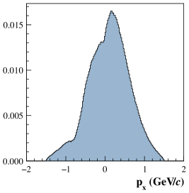
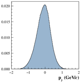
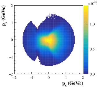
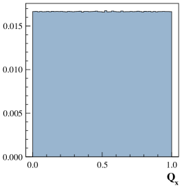
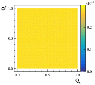
Figure 1: Example of the effect of the cumulative transformation of transverse momentum components, $p_{x}$ and $p_{y}$ of proton candidates selected for intermittency analysis of the NA61/SHINE ⁴⁰Ar + ⁴⁵Sc at 150A GeV/c data. Distributions before (top) and after (bottom) the transformation.

Both methods are approximate. Subtracting moments for mixed data set may introduce negative $\Delta F_{2}(M)$ values [11] and using cumulative quantities mixes the scales of the momentum differences and therefore may distort eventual power-law behavior.

3 The NA61/SHINE detector

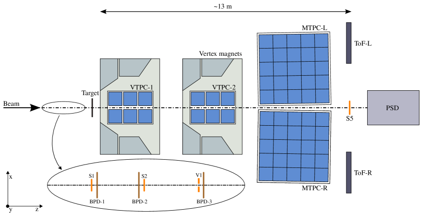
Figure 2: The schematic layout of the NA61/SHINE experiment at the CERN SPS  [1] showing the components used for the ⁴⁰Ar + ⁴⁵Sc energy scan (horizontal cut, not to scale). The detector configuration upstream of the target is shown in the inset. Alignment of the chosen coordinate system is shown on the plot; its origin (x=y=z=0) lies in the middle of VTPC-2, on the beam axis. The nominal beam direction is along the z-axis. Target is placed at z $\approx-580$ cm. The magnetic field bends charged particle trajectories in the x–z (horizontal) plane. The drift direction in the TPCs is along the (vertical) y-axis.

The NA61/SHINE detector (see Fig. 2) is a large-acceptance hadron spectrometer situated in the North Area H2 beam-line of the CERN SPS [1]. The main components of the detection system used in the analysis are four large-volume Time Projection Chambers (TPC). Two of them, called Vertex TPCs (VTPC-1/2), are located downstream of the target inside superconducting magnets with maximum combined bending power of 9 Tm, which was set for the data collection at 150A GeV/c. The main TPCs (MTPC-L/R) and two walls of pixel Time-of-Flight (ToF-L/R) detectors are placed symmetrically on either side of the beamline downstream of the magnets. The TPCs are filled with Ar:CO₂ gas mixtures in proportions 90:10 for the VTPCs and 95:5 for the MTPCs. The Projectile Spectator Detector (PSD), a zero-degree hadronic calorimeter, is positioned 16.7 m downstream of the MTPCs, centered in the transverse plane on the deflected position of the beam. It consists of 44 modules that cover a transverse area of almost 2.5 m². The central part of the PSD consists of 16 small modules with transverse dimensions of 10 x 10 cm² and its outer part consists of 28 large 20 x 20 cm² modules. Moreover, a brass cylinder of 10 cm length and 5 cm diameter (degrader) was placed in front of the center of the PSD in order to reduce electronic saturation effects and shower leakage from the downstream side caused by the Ar beam and its heavy fragments.

Primary beams of fully ionized ⁴⁰Ar nuclei were extracted from the SPS accelerator at 150A GeV/c beam momentum. Two scintillation counters, S1 and S2, provide beam definition, together with a veto counter V1 with a 1 cm diameter hole, which defines the beam before the target. The S1 counter also provides the timing reference (start time for all counters). Beam particles are selected by the trigger system requiring the coincidence $\textrm{T1}=\textrm{S1}\wedge\textrm{S2}\wedge\overline{\textrm{V1}}$. Individual beam particle trajectories are precisely measured by the three beam position detectors (BPDs) placed upstream of the target [1]. Collimators in the beam line were adjusted to obtain beam rates of $\approx 10^{4}$/s during the $\approx$ 10 s spill and a super-cycle time of 32.4 s.

The target was a stack of 2.5 x 2.5 cm² area and 1 mm thick ⁴⁵Sc plates of 6 mm total thickness placed $\approx$ 80 cm upstream of VTPC-1. Impurities due to other isotopes and elements were measured to be 0.3% [29]. No correction was applied for this negligible contamination.

Interactions in the target are selected with the trigger system by requiring an incoming ⁴⁰Ar ion and a signal below that of beam ions from S5, a small 2 cm diameter scintillation counter placed on the beam trajectory behind the MTPCs. This minimum bias trigger is based on the breakup of the beam ion due to interactions in and downstream of the target. In addition, central collisions were selected by requiring an energy signal below a set threshold from the 16 central modules of the PSD, which measure mainly the energy carried by projectile spectators. The cut was set to retain only the events with the $\approx$ 30% smallest energies in the PSD. The event trigger condition thus was $\textrm{T2}=\textrm{T1}\wedge\overline{\textrm{S5}}\wedge\overline{\textrm{PSD}}$. The statistics of recorded events at 150A GeV/c are summarized in Table 1.

Table 1: Basic beam properties and number of events recorded and used in the analysis of ⁴⁰Ar + ⁴⁵Sc interactions at incident momentum of 150A GeV/c.

$p_{beam}$ (GeV/c)	$\sqrt{s_{\mathrm{NN}}}$ (GeV)	Recorded central triggers	Number of selected events
150A	16.84	$1.7\cdot 10^{6}$	$1.1\cdot 10^{6}$

4 Analysis

The goal of the analysis was to search for the critical point of the strongly interacting matter by measuring the second-order scaled factorial moments for a selection of protons produced in central ⁴⁰Ar + ⁴⁵Sc interactions at 150A GeV/c, using statistically independent points and cumulative variables.

4.1 Event selection

NA61/SHINE detector recorded over 1.7 million collisions using 150A GeV/c ⁴⁰Ar beam impinging on a stationary ⁴⁵Sc target. However, not all of those events contain well-reconstructed central Ar+Sc interactions. Therefore the following criteria were used to select data for further analysis.

1. no off-time beam particle detected within a time window of $\pm 4\mu$s around the trigger particle,

2. no interaction-event trigger detected within a time window of $\pm 25\mu$s around the trigger particle,

3. beam particle detected in at least two planes out of four of BPD-1 and BPD-2 and in both planes of BPD-3,

4. T2 trigger (set to select central and semi-central collisions),

5. a high-precision interaction vertex with z position (fitted using the beam trajectory and TPC tracks) no further than 10 cm away from the center of the Sc target (the cut removes less than 0.4% of T2 trigger ($E_{PSD}$) selected interactions),

6. energy in small PSD modules should be less than 2800 GeV,

7. energy in large PSD modules should be in the range between 800 GeV and 5000 GeV,

8. if the number of tracks in the vertex fit is less than 50, then the ratio of tracks in fit to all tracks must be at least 0.25.

After applying the selection criteria, about 1.1 million events remain for further analysis.

4.2 Centrality selection

The analysis was performed in several centrality intervals (0-5%, 5-10%, 10-15%, 15-20% and 0-20%). Centrality is determined using the energy deposited in the PSD forward calorimeter, $E_{PSD}$ (see Ref. [30] for details). Figure 3 shows the proton candidate multiplicity distributions for each of the studied centrality classes and the distributions of the number of accepted proton candidates for different selections of energy deposited in PSD.

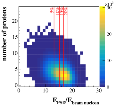
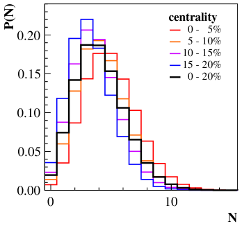
Figure 3: Left: Distribution of selected events in the number of accepted proton candidates and the energy registered by the Particle Spectator Detector with PSD-energy values for centrality selection marked as red vertical lines. Right: Multiplicity distributions of proton candidates for different centrality selections (for all events selected for the analysis and after all track cuts described in Sec. 4.3).

Table 2 presents number of events in each of the chosen centrality intervals selected for the analysis.

Table 2: Number of events selected for the analysis.

data set	number of events in centrality intervals
	0 – 5%	5 – 10%	10 – 15%	15 – 20%	0 – 20%
experimental data	237k	235k	236k	216k	924k
Epos1.99	323k	323k	323k	324k	1293k

4.3 Single-track selection

To select tracks of primary charged hadrons and to reduce the contamination by particles from secondary interactions, weak decays and off-time interactions, the following track selection criteria were applied:

1. track momentum fit including the interaction vertex should have converged,

2. total number of reconstructed points on the track should be greater than 30,

3. sum of the number of reconstructed points in VTPC-1 and VTPC-2 should be greater than 15,

4. the ratio of the number of reconstructed points to the potential (maximum possible) number of reconstructed points should be greater than 0.5 and less than 1.1,

5. number of points used to calculate energy loss ($\textrm{d}E\!/\!\textrm{d}x$) should be greater than 30,

6. the distance between the track extrapolated to the interaction plane and the vertex (track impact parameter) should be smaller than 4 cm in the horizontal (bending) plane and 2 cm in the vertical (drift) plane.

As the analysis concerns mid-rapidity protons, only particles with center-of-mass rapidity (assuming proton mass) greater than -0.75 and less than 0.75 were considered.

Only particles with transverse momentum components, $p_{x}$ and $p_{y}$, absolute values less than 1.5 GeV/c were accepted for the analysis.

4.3.1 Proton selection

To identify proton candidates, positively charged particles were selected. Their ionization energy loss in TPCs is taken to be greater than 0.5 and less than the proton Bethe-Bloch value increased by the 15% difference between the values for kaons and protons while the momentum is in the relativistic-rise region (from 4 to 125 GeV/c). The $\textrm{d}E\!/\!\textrm{d}x$ distribution for selected positive particles is shown in Fig. 4. The selected region is marked with a red line.

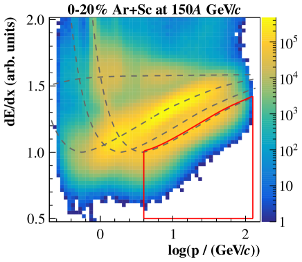
Figure 4: Energy loss vs total momentum of positively charged particles measured with the NA61/SHINE Time Projection Chambers in the selected ⁴⁰Ar + ⁴⁵Sc events at 150A GeV/c. Dashed lines represent the nominal Bethe-Bloch values. The graphical cut to select proton candidates is marked with a red line.

The selection was found to select, on average, approximately 60% of protons and leave, on average, less than 4% of kaon contamination. The corresponding random proton losses do not bias the final results in case of independent production of protons in the transverse momentum space. The results for correlated protons will be biased by the selection (see Sec. 5 for an example), thus the random proton selection should be considered when calculating model predictions.

4.4 Acceptance maps

4.4.1 Single-particle acceptance map

A three-dimensional (in $p_{x}$, $p_{y}$ and center-of-mass rapidity) acceptance map [31] was created to describe the momentum region selected for this analysis. The map was created by comparing the number of Monte Carlo-generated mid-rapidity protons before and after detector simulation and reconstruction. Only particles from the regions with at least 70% reconstructed tracks are analyzed. The single-particle acceptance maps should be used for calculating model predictions.

4.4.2 Two-particle acceptance map

Time Projection Chambers (the main tracking devices of NA61/SHINE) are not capable of distinguishing tracks that are too close to each other in space. At a small distance, their clusters overlap, and signals are merged.

The mixed data set is constructed by randomly swapping particles from different events so that each particle in each mixed event comes from different recorded events.

For each pair of particles in both recorded and mixed events, a Two-Track Distance (TTD) is calculated. It is an average distance of their tracks in $p_{x}$-$p_{y}$ plane at eight different $z$ planes (-506, -255, -201, -171, -125, 125, 352 and 742 cm). Figure 5 presents TTD distributions for both data sets (left) and their ratio (right). The TPC’s limitation to recognizing close tracks is clearly visible for TTD < 2 cm.

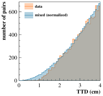
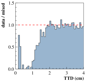
Figure 5: Distributions of Two-Track Distance for experimental and mixed data (left) and their ratio (right).

Calculating TTD requires knowledge of the NA61/SHINE detector geometry and magnetic field. Hence it is restricted to the Collaboration members. Therefore, a momentum-based Two-Track Distance (mTTD) cut was introduced to allow for a meaningful comparison with models.

The magnetic field bends the trajectory of charged particles in the x-z plane. Thus, it is most convenient to express the momentum of each positive particle in both recorded and mixed data sets in the following coordinates:

$$s_{x} =p_{x}/p_{xz},$$

$$s_{y} =p_{y}/p_{xz},$$

$$\rho =1/p_{xz},$$

where $p_{xz}=\sqrt{p_{x}^{2}+p_{z}^{2}}$. For each pair of positively charged particles, a difference in these coordinates is calculated as

$$\Delta s_{x} =s_{x,2}-s_{x,1},$$

$$\Delta s_{y} =s_{y,2}-s_{y,1},$$

$$\Delta\rho =\rho_{2}-\rho_{1}.$$

The distribution of particle pairs’ momentum difference for pairs with TTD < 2 cm is parametrized with ellipses in the new coordinates. Such elliptic cuts are applied to recorded and mixed events. Their distributions and their ratio are shown in Fig. 6.

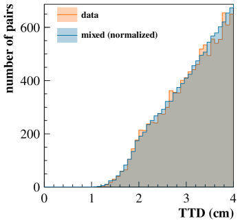
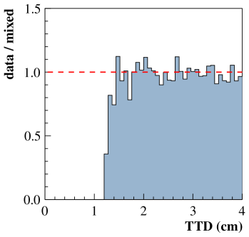
Figure 6: Distributions of Two-Track Distance for experimental and mixed data (left) and their ratio (right) after applying the momentum-based Two-Track Distance cut.

The mTTD cut defines the two-particle acceptance used in the analyses. The explicit formulas with numerical values of parameters are:

$$\left(\frac{\Delta\rho}{0.0105}\right)^{2}+\left(\frac{\Delta s_{y}}{0.0018}\right)^{2} \leq 1,$$

$$\left(\frac{\Delta s_{x}}{0.0080}\right)^{2}+\left(\frac{\Delta s_{y}}{0.0018}\right)^{2} \leq 1,$$

$$\left(\frac{\Delta\rho\cos(\text{51}^{\circ})-\Delta s_{x}\sin(\text{51}^{\circ})}{0.0200}\right)^{2}+\left(\frac{\Delta\rho\sin(\text{51}^{\circ})+\Delta s_{x}\cos(\text{51}^{\circ})}{0.0023}\right)^{2} \leq 1.$$

Particle pairs with momenta inside all the ellipses are rejected. The two-particle acceptance maps should be used for calculating model predictions.

4.5 Statistically-independent data points

The intermittency analysis yields the dependence of scaled factorial moments on the number of subdivisions of transverse momentum and cumulative transverse momentum intervals. In the past, the same data set was used for the analysis performed for different subdivision numbers. This resulted in statistically-correlated data points uncertainties, therefore the full covariance matrix is required for proper statistical treatment of the results. The latter may be numerically not trivial [32]. Here, for the first time, statistically-independent data subsets were used to obtain results for each subdivision number. In this case, the results for different subdivision numbers are statistically independent. Only diagonal elements of the covariance matrix are non-zero, and thus the complete relevant information needed to interpret the results is easy to present graphically and use in the statistical tests. However, the procedure significantly decreases the number of events used to calculate each data point increasing statistical uncertainties and therefore forcing to reduce the number of the data points to 10.

Number of events used in each subset was selected to obtain similar magnitudes of the statistical uncertainties of results for different subsets. Table 3 presents the fractions of all available events used to calculate each of the 10 points.

Table 3: Fraction of the total number of analyzed events for each centrality interval used to calculate second-order scaled factorial moments for the chosen number of cumulative momentum cells.

number of cells $M^{2}$	$1^{2}$	$50^{2}$	$70^{2}$	$86^{2}$	$100^{2}$	$111^{2}$	$122^{2}$	$132^{2}$	$141^{2}$	$150^{2}$
fraction of all events (%)	0.5	3.0	5.0	7.0	9.0	11.0	13.0	15.5	17.0	19.0

4.6 Uncertainties and biases

The standard expression for the scaled factorial moments, Eq. 1 can be rewritten as

$$F_{2}(M)=2M^{2}\frac{\langle N_{2}(M)\rangle}{\langle N\rangle^{2}},$$ (7)

where $N_{2}(M)$ denotes the total number of particle pairs in all of the $M^{2}$ bins in an event. Then the statistical uncertainties can be calculated using the standard error propagation:

$$\frac{\sigma_{F_{2}}}{|F_{2}|}=\sqrt{\frac{(\sigma_{N_{2}})^{2}}{\langle N_{2}\rangle^{2}}+4\frac{(\sigma_{N})^{2}}{\langle N\rangle^{2}}-4\frac{(\sigma_{N_{2}N})^{2}}{\langle N\rangle\langle N_{2}\rangle}}.$$ (8)

The left plot in Fig. 7 shows $F_{2}(M)$ results for the mixed data set (see Sec. 5 for details). As expected, the $F_{2}$ values are independent of $M^{2}$. Deviation of the points from the value for the first point (marked with the dashed line) is approximately $\chi^{2}\kern-3.00003pt/\kern-1.00006pt\text{ndf}$ = 7.7/9, which validates the values of statistical uncertainties.

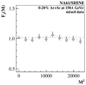
Figure 7: Results on the dependence of the scaled factorial moment of proton multiplicity distribution on the number of subdivisions in cumulative transverse momentum space for mixed events (left) as well as events generated with Epos1.99 model before and after reconstruction (right).

Final results presented in Sec. 5 are not corrected for possible biases. Systematic uncertainty was estimated by comparing results for pure Epos1.99 and Epos1.99 subjected to the detector simulation, reconstruction and data-like analysis as shown in Fig. 7 (right). Their differences are significantly smaller than statistical uncertainties ($\chi^{2}\kern-3.00003pt/\kern-1.00006pt\text{ndf}$ = 9.7/9) of the experimental data and increase with $M^{2}$ up to the order of 0.1 at large $M^{2}$ values. Note that protons generated by Epos1.99 do not show significant correlation in the transverse momentum space, see Sec. 6. In this case, the momentum resolution does not affect the results significantly.

In the case of the critical correlations, the impact of the momentum resolution may be significant, see Ref. [33] and Sec. 6 for detail. Thus a comparison with models including short-range correlations in the transverse momentum space requires smearing of their momenta according to the the experimental resolution, which can be approximately parametrized as:

$$\begin{split}p_{x}^{\text{smeared}}&=p_{x}^{\text{original}}+\delta p,\\ p_{y}^{\text{smeared}}&=p_{y}^{\text{original}}+\delta p,\end{split}$$ (9)

where $\delta p$ is randomly drawn from a Gaussian distribution with $\sigma=3$ MeV/c.

Uncertainties on final results presented in Sec. 5 correspond to statistical uncertainties.

5 Results

This section presents results on second-order scaled factorial moments (Eq. 1) of $\approx 60\%$ randomly selected protons (losses due to proton misidentification) with momentum smeared due to reconstruction resolution (Eq. 9) produced within the acceptance maps defined in Sec. 4.4 by strong and electromagnetic processes in 0-5%, 5-10%, 10-15%, 15-20% and 0-20% most central ⁴⁰Ar + ⁴⁵Sc collisions at 150A GeV/c. The results are shown as a function of the number of subdivisions in transverse momentum space – the so-called intermittency analysis. The analysis was performed for cumulative and original transverse momentum components. Independent data sets were used to calculate results for each subdivision.

Uncertainties correspond to statistical ones. Biases estimated using the Epos1.99 [34] model (see Sec. 6) are significantly smaller than statistical uncertainties of the experimental data.

5.1 Subdivisions in cumulative transverse momentum space

Figures 8 and 9 present the dependence of the factorial moment on the number of subdivisions in cumulative-transverse momentum space for the maximum subdivision number of $M^{2}=150^{2}$ and $M^{2}=32^{2}$, respectively. The latter, coarse subdivision, was introduced to limit the effect of experimental momentum resolution; see Ref. [33] and below for details. The experimental results are shown for five different selections of events with respect to centrality. As a reference, the corresponding results for mixed events are also shown. The mixed data set is constructed by randomly swapping particles from different events such that each particle in a mixed event comes from different recorded events. Note that by construction, the multiplicity distribution of protons in mixed events for $M^{2}=1^{2}$ is equal to the corresponding distribution for the data. In the mixed events, protons are uncorrelated in the transverse momentum space. Therefore for them, the scaled factorial moment is independent of $M^{2}$, $F_{2}(M)=F_{2}(1^{2})$. The experimental results do not show any significant dependence on $M^{2}$. The obtained values are consistent with the value of the first data point (dashed line) with $\chi^{2}\kern-3.00003pt/\kern-1.00006pt\text{ndf}$ = 8.7/9 on average for the fine binning (Fig. 8) and $\chi^{2}\kern-3.00003pt/\kern-1.00006pt\text{ndf}$ = 11.4/9 for the coarse binning (Fig. 9). There is no indication of the critical fluctuations for selected protons.

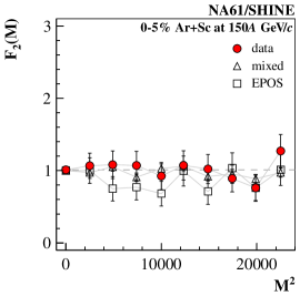
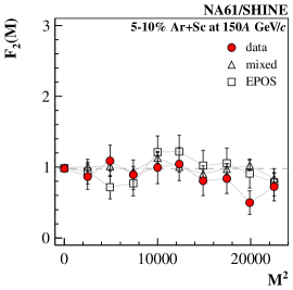
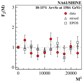
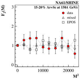
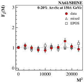
Figure 8: Results on the dependence of the scaled factorial moment of proton multiplicity distribution on the number of subdivisions in cumulative transverse momentum space $M^{2}$ for $1^{2}\leq M^{2}\leq 150^{2}$. Closed circles indicate the experimental data. For comparison, corresponding results for mixed events (open triangles) and the Epos1.99 model (open squares) are also shown. Results for five centrality selections of events are presented in different panels. Only statistical uncertainties are indicated.

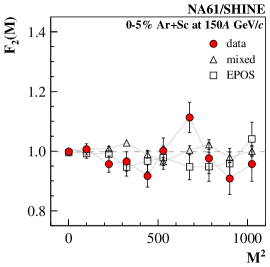
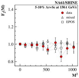
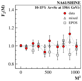
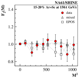
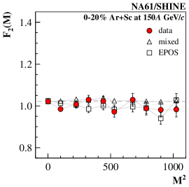
Figure 9: Results on the dependence of the scaled factorial moment of proton multiplicity distribution on the number of subdivisions in cumulative transverse momentum space $M^{2}$ for $1^{2}\leq M^{2}\leq 32^{2}$. Closed circles indicate the experimental data. For comparison, corresponding results for mixed events (open triangles) and the Epos1.99 model (open squares) are also shown. Results for five centrality selections of events are presented in different panels. Only statistical uncertainties are indicated.

5.2 Subdivisions in transverse momentum space

Figure 10 presents the results which correspond to the results shown in Fig. 8, but subdivisions are done in the original transverse momentum space. By construction, $F_{2}(1^{2})$ values are equal for subdivisions in cumulative transverse momentum space and transverse momentum space. But for the latter, $F_{2}(M)$ strongly depends on $M^{2}$. This dependence is primarily due to non-uniform shape of the single-particle transverse momentum distributions, see Sec. 2.2. It can be accounted for by comparing the results for the experimental data with the corresponding results obtained for the mixed events. There is no significant difference between the two, which confirms the previous conclusion of no indication of significant critical fluctuations.

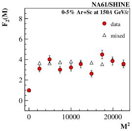
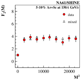
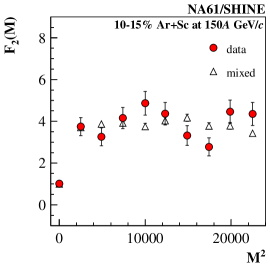
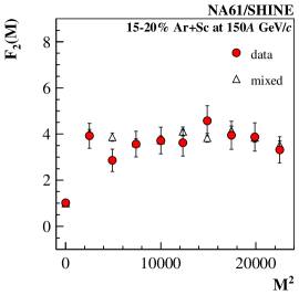
Figure 10: Results on the dependence of the scaled factorial moment of proton multiplicity distribution on the number of subdivisions in transverse momentum space $M^{2}$ for $1^{2}\leq M^{2}\leq 150^{2}$. Closed circles indicate the experimental data. For comparison, corresponding results for mixed events (open triangles) are also shown. Results for five centrality selections of events are presented in different panels. Only statistical uncertainties are indicated.

6 Comparison with models

This section presents a comparison of the experimental results with two models. The first one, Epos1.99 [34], takes into account numerous sources of particle correlations, in particular, conservation laws and resonance decays, but without critical fluctuations. The second one, the Power-law Model [35], produces particles correlated by the power law together with fully uncorrelated particles.

6.1 Epos

For comparison, almost $20\cdot 10^{6}$ minimum bias ⁴⁰Ar + ⁴⁵Sc events have been generated with Epos1.99. Signals from the NA61/SHINE detector were simulated with Geant3 software, and the recorded events were reconstructed using the standard NA61/SHINE procedure. Number of analyzed events is shown in Table 2.

To calculate model predictions (pure Epos), all generated central events were analyzed. Protons and proton pairs within the single-particle and two-particle acceptance maps were selected. Moreover, 60% of accepted protons were randomly selected for the analysis to take into account the effect of the proton misidentification.

Results for the reconstructed Epos events were obtained as follows. The model events were required to have the reconstructed primary vertex. Selected protons and proton pairs (matching to the generated particles was used for identification) were subject to the same cuts as used for the experimental data analysis, see Sec. 4.

The results for the pure and the reconstructed Epos events are compared in Fig. 11. They agree for both fine and coarse subdivisions. As the statistics of the Epos events is several times higher than of the data, one concludes that for the Epos-like physics, the biases of the experimental data are significantly smaller than the statistical uncertainties of the data.

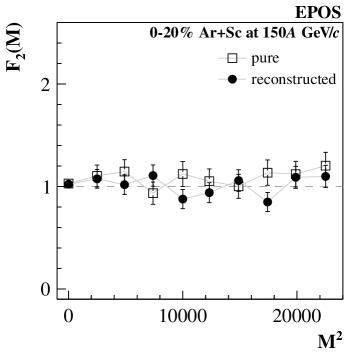
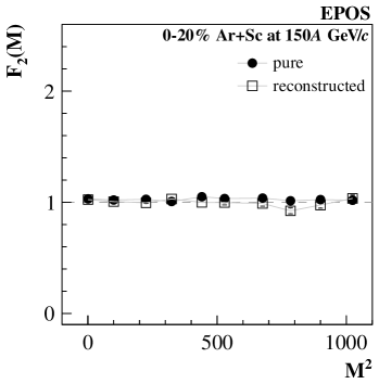
Figure 11: Results on the dependence of the scaled factorial moment of proton multiplicity distribution on the number of subdivisions in cumulative transverse momentum space for events generated with Epos1.99 for fine $M^{2}=1^{2}...150^{2}$ (left) and coarse, $M^{2}=1^{2}...32^{2}$ (right) subdivisions.

Finally, the experimental results are compared with the pure Epos predictions in Figs. 8, 9 and 10. No significant differences are found.

6.2 Power-law Model

Inspired by expectations of the power-law correlations between particles near the critical point, the Power-law Model was developed [35] to compare with the experimental result. It generates momenta of uncorrelated and correlated protons with a given single-particle transverse momentum distribution in events with a given multiplicity distribution. The model has two controllable parameters:

1. fraction of correlated particles,

2. strength of the correlation (the power-law exponent).

The transverse momentum of particles is drawn from the input transverse momentum distribution. Correlated-particle pairs’ transverse momentum difference follows a power-law distribution:

$$\rho(|\Delta\overrightarrow{p_{T}}|)\sim|\Delta\overrightarrow{p_{T}}|^{-\phi_{2}},$$ (10)

where the exponent $\phi_{2}<1$. Azimuthal-angle distribution is assumed to be uniform. The momentum component along the beamline, $p_{z}$, is calculated assuming a uniform rapidity distribution from $-0.75$ to $0.75$ and proton mass.

Many high-statistics data sets with multiplicity distributions identical to the experimental data and similar inclusive transverse momentum distributions have been produced using the model. Each data set has a different fraction of correlated particles (varying from 0 to 2%) and a different power-law exponent (varying from 0.00 to 0.95). The following effects have been included:

1. Gaussian smearing of momentum components to mimic reconstruction resolution of the momentum, (see Eq. 9),

2. random exchange of 40% of correlated particles with uncorrelated ones to simulate 60% acceptance of protons (preserves the desired multiplicity distribution, but requires generating more correlated pairs at the beginning),

3. two-particle acceptance map, see Sec. 4.4,

4. single-particle acceptance map, see Sec. 4.4.

The influence of each of the above effects separately and all of them applied together on $F_{2}(M)$ is shown in Fig. 12 for an example model parameters, and fine and coarse subdivisions.

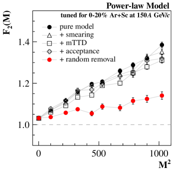
Figure 12: Dependence of the scaled factorial moment on the number of subdivisions in the cumulative transverse momentum for the Power-law Model with power-law exponent set to 0.80 and fraction of correlated particles to 3%. Each line presents a result with a different effect included separately, and the red circles all of them together. The results for the fine and coarse subdivisions are shown in the left and right panels, respectively.

Next, all generated data sets with all the above effects included have been analyzed the same way as the experimental data. Obtained $F_{2}(M)$ results have been compared with the corresponding experimental results and $\chi^{2}$ and a p-value were calculated. For the calculation, statistical uncertainties from the model with similar statistics to the data were used. Examples of such comparison are presented in Fig. 13.

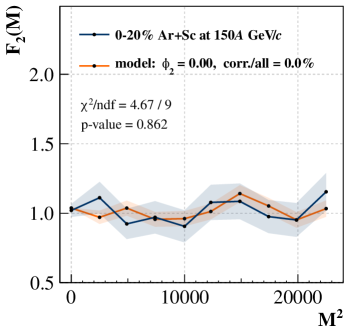
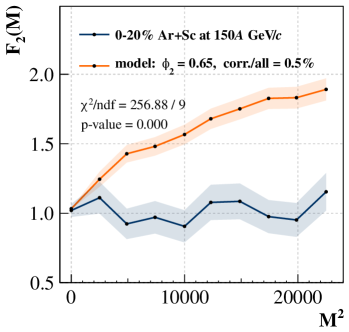
Figure 13: Examples of comparison of results for two Power-law Model data sets with the experimental data. The left panel includes model predictions assuming only uncorrelated protons, whereas the right one shows predictions for 0.5% of correlated protons with power-law exponent $\phi_{2}=0.65$.

Figure 14 shows obtained p-values as a function of the fraction of correlated protons and the power-law exponent.

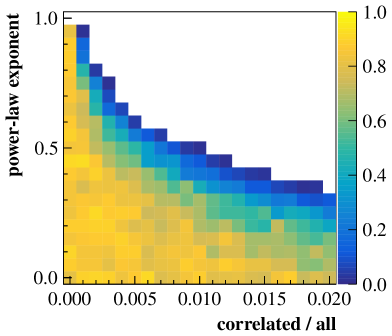
Figure 14: Exclusion plot, the p-values, for the Power-law Model parameters – the fraction of correlated protons and the power-law exponent. The white areas correspond to p-values less than 1%. The exclusion plot for the fine subdivisions.

White areas correspond to a p-value of less than 1% and may be considered excluded (for this particular model). Results for the coarse subdivision have low statistical uncertainties, thus small deviations from the behavior expected for uncorrelated particle production due to non-critical correlations (conservation laws, resonance decays, quantum statistics, …), as well as possible experimental biases may lead to significant decrease of the p-values.

The intermittency index $\phi_{2}$ for an infinite system at the QCD critical point is expected to be $\phi_{2}$ = 5/6, assuming that the latter belongs to the 3-D Ising universality class. If this value is set as the power-law exponent of the Power-law Model with coarse subdivisions (Fig. 14), the NA61/SHINE data on central ⁴⁰Ar + ⁴⁵Sc collisions at 150A GeV/c exclude fractions of correlated protons larger than about 0.1%.

7 Summary

This paper reports on the search for the critical point of strongly interacting matter in central ⁴⁰Ar + ⁴⁵Sc collisions at 150A GeV/c. Results on second-order scaled factorial moments of proton multiplicity distribution at mid-rapidity are presented. Protons produced in strong and electromagnetic processes in ⁴⁰Ar + ⁴⁵Sc interactions and selected by the single- and two-particle acceptance maps, as well as the identification cuts are used.

The scaled factorial moments are shown as a function of the number of subdivisions of transverse momentum space – the so-called intermittency analysis. The analysis was performed for cumulative and non-cumulative transverse momentum components. Independent data sets were used to calculate results for each subdivision. Influence of several experimental effects was discussed and quantified. The results show no significant intermittency signal.

The experimental data are consistent with the mixed events and the Epos model predictions. An upper limit on the fraction of critical proton pairs and the power of the correlation function was obtained based on a comparison with the Power-law Model.

The intermittency analysis of other reactions recorded within the NA61/SHINE program on strong interactions is well advanced and the new final results should be expected soon.

The NA61/SHINE Collaboration

H. Adhikary¹⁴, P. Adrich¹⁶, K.K. Allison²⁷, N. Amin⁵, E.V. Andronov²³, T. Antićić³, I.-C. Arsene¹³, M. Bajda¹⁷, Y. Balkova¹⁹, M. Baszczyk¹⁸, D. Battaglia²⁶, A. Bazgir¹⁴, S. Bhosale¹⁵, M. Bielewicz¹⁶, A. Blondel⁴, M. Bogomilov², Y. Bondar¹⁴, N. Bostan²⁶, A. Brandin²³, W. Bryliński²², J. Brzychczyk¹⁷, M. Buryakov²³, A.F. Camino²⁹, P. Christakoglou⁷, M. Ćirković²⁴, M. Csanád⁹, J. Cybowska²², T. Czopowicz¹⁴, C. Dalmazzone⁴, N. Davis¹⁵, F. Diakonos⁷, A. Dmitriev²³, P. von Doetinchem²⁸, W. Dominik²⁰, P. Dorosz¹⁸, J. Dumarchez⁴, R. Engel⁵, G.A. Feofilov²³, L. Fields²⁶, Z. Fodor^8,21, M. Friend¹⁰, M. Gaździcki^14,6, O. Golosov²³, V. Golovatyuk²³, M. Golubeva²³, K. Grebieszkow²², F. Guber²³, S.N. Igolkin²³, S. Ilieva², A. Ivashkin²³, A. Izvestnyy²³, K. Kadija³, A. Kapoyannis⁷, N. Kargin²³, N. Karpushkin²³, E. Kashirin²³, M. Kiełbowicz¹⁵, V.A. Kireyeu²³, H. Kitagawa¹¹, R. Kolesnikov²³, D. Kolev², Y. Koshio¹¹, V.N. Kovalenko²³, S. Kowalski¹⁹, B. Kozłowski²², A. Krasnoperov²³, W. Kucewicz¹⁸, M. Kuchowicz²¹, M. Kuich²⁰, A. Kurepin²³, A. László⁸, M. Lewicki²¹, G. Lykasov²³, V.V. Lyubushkin²³, M. Maćkowiak-Pawłowska²², Z. Majka¹⁷, A. Makhnev²³, B. Maksiak¹⁶, A.I. Malakhov²³, A. Marcinek¹⁵, A.D. Marino²⁷, H.-J. Mathes⁵, T. Matulewicz²⁰, V. Matveev²³, G.L. Melkumov²³, A. Merzlaya¹³, Ł. Mik¹⁸, A. Morawiec¹⁷, S. Morozov²³, Y. Nagai⁹, T. Nakadaira¹⁰, M. Naskręt²¹, S. Nishimori¹⁰, V. Ozvenchuk¹⁵, A.D. Panagiotou⁷, O. Panova¹⁴, V. Paolone²⁹, O. Petukhov²³, I. Pidhurskyi^14,6, R. Płaneta¹⁷, P. Podlaski²⁰, B.A. Popov^23,4, B. Pórfy^8,9, M. Posiadała-Zezula²⁰, D.S. Prokhorova²³, D. Pszczel¹⁶, S. Puławski¹⁹, J. Puzović^24†, R. Renfordt¹⁹, L. Ren²⁷, V.Z. Reyna Ortiz¹⁴, D. Röhrich¹², E. Rondio¹⁶, M. Roth⁵, Ł. Rozpłochowski¹⁵, B.T. Rumberger²⁷, M. Rumyantsev²³, A. Rustamov^1,6, M. Rybczynski¹⁴, A. Rybicki¹⁵, K. Sakashita¹⁰, K. Schmidt¹⁹, A.Yu. Seryakov²³, P. Seyboth¹⁴, U.A. Shah¹⁴, Y. Shiraishi¹¹, A. Shukla²⁸, M. Słodkowski²², P. Staszel¹⁷, G. Stefanek¹⁴, J. Stepaniak¹⁶, M. Strikhanov²³, H. Ströbele⁶, T. Šuša³, L. Swiderski¹⁶, J. Szewiński¹⁶, R. Szukiewicz²¹, A. Taranenko²³, A. Tefelska²², D. Tefelski²², V. Tereshchenko²³, A. Toia⁶, R. Tsenov², L. Turko²¹, T.S. Tveter¹³, M. Unger⁵, M. Urbaniak¹⁹, F.F. Valiev²³, M. Vassiliou⁷, D. Veberič⁵, V.V. Vechernin²³, V. Volkov²³, A. Wickremasinghe²⁵, K. Wójcik¹⁹, O. Wyszyński¹⁴, A. Zaitsev²³, E.D. Zimmerman²⁷, A. Zviagina²³, and R. Zwaska^25
 
† deceased

¹ National Nuclear Research Center, Baku, Azerbaijan
² Faculty of Physics, University of Sofia, Sofia, Bulgaria
³ Ruđer Bošković Institute, Zagreb, Croatia
⁴ LPNHE, University of Paris VI and VII, Paris, France
⁵ Karlsruhe Institute of Technology, Karlsruhe, Germany
⁶ University of Frankfurt, Frankfurt, Germany
⁷ University of Athens, Athens, Greece
⁸ Wigner Research Centre for Physics, Budapest, Hungary
⁹ Eötvös Loránd University, Budapest, Hungary
¹⁰ Institute for Particle and Nuclear Studies, Tsukuba, Japan
¹¹ Okayama University, Japan
¹² University of Bergen, Bergen, Norway
¹³ University of Oslo, Oslo, Norway
¹⁴ Jan Kochanowski University, Kielce, Poland
¹⁵ Institute of Nuclear Physics, Polish Academy of Sciences, Cracow, Poland
¹⁶ National Centre for Nuclear Research, Warsaw, Poland
¹⁷ Jagiellonian University, Cracow, Poland
¹⁸ AGH - University of Science and Technology, Cracow, Poland
¹⁹ University of Silesia, Katowice, Poland
²⁰ University of Warsaw, Warsaw, Poland
²¹ University of Wrocław, Wrocław, Poland
²² Warsaw University of Technology, Warsaw, Poland
²³ Affiliated with an institution covered by a cooperation agreement with CERN
²⁴ University of Belgrade, Belgrade, Serbia
²⁵ Fermilab, Batavia, USA
²⁶ University of Notre Dame, Notre Dame, USA
²⁷ University of Colorado, Boulder, USA
²⁸ University of Hawaii at Manoa, Honolulu, USA
²⁹ University of Pittsburgh, Pittsburgh, USA

References

- [1] N. Abgrall et al., [NA61/SHINE Collab.] JINST 9 (2014) P06005, arXiv:1401.4699 [physics.ins-det].
- [2] A. Aduszkiewicz, [NA61/SHINE Collab.], “Report from the NA61/SHINE experiment at the CERN SPS,” Tech. Rep. CERN-SPSC-2018-029. SPSC-SR-239, CERN, Geneva, Oct, 2018. https://cds.cern.ch/record/2642286.
- [3] N. G. Antoniou, F. K. Diakonos, A. S. Kapoyannis, and K. S. Kousouris Phys. Rev. Lett. 97 (2006) 032002, arXiv:hep-ph/0602051 [hep-ph].
- [4] J. Wosiek Acta Phys. Polon. B19 (1988) 863–866.
- [5] S. Afanasiev et al., [NA49 Collab.] Phys. Rev. C66 (2002) 054902.
- [6] C. Alt et al., [NA49 Collab.] Phys. Rev. C77 (2008) 024903.
- [7] A. Bialas and R. B. Peschanski Nucl. Phys. B273 (1986) 703–718.
- [8] H. Satz Nucl. Phys. B326 (1989) 613–618.
- [9] N. G. Antoniou, E. N. Argyres, C. G. Papadopoulos, A. P. Contogouris, and S. D. P. Vlassopulos Phys. Lett. B245 (1990) 619–623.
- [10] A. Bialas and R. Hwa Phys. Lett. B253 (1991) 436–438.
- [11] T. Anticic et al., [NA49 Collab.] Eur. Phys. J. C 75 no. 12, (2015) 587, arXiv:1208.5292 [nucl-ex].
- [12] M. A. Stephanov, K. Rajagopal, and E. V. Shuryak Phys. Rev. Lett. 81 (1998) 4816–4819, arXiv:hep-ph/9806219 [hep-ph].
- [13] M. A. Stephanov, K. Rajagopal, and E. V. Shuryak Phys. Rev. D60 (1999) 114028, arXiv:hep-ph/9903292 [hep-ph].
- [14] A. Bialas and M. Gazdzicki Phys. Lett. B 252 (1990) 483–486.
- [15] S. Samanta, T. Czopowicz, and M. Gazdzicki Nucl. Phys. A 1015 (2021) 122299, arXiv:2105.00344 [nucl-th].
- [16] A. Bialas and J. Seixas Phys. Lett. B250 (1990) 161–163.
- [17] W. Ochs and J. Wosiek Phys. Lett. B214 (1988) 617–620.
- [18] W. Ochs Phys. Lett. B247 (1990) 101–106.
- [19] N. Antoniou, Y. Contoyiannis, F. Diakonos, A. Karanikas, and C. Ktorides Nucl. Phys. A693 (2001) 799–824, arXiv:hep-ph/0012164 [hep-ph].
- [20] M. A. Stephanov Prog. Theor. Phys. Suppl. 153 (2004) 139–156, arXiv:hep-ph/0402115 [hep-ph]. [Int. J. Mod. Phys.A20,4387(2005)].
- [21] N. Antoniou, Y. Contoyiannis, F. Diakonos, and G. Mavromanolakis Nucl. Phys. A761 (2005) 149–161, arXiv:hep-ph/0505185 [hep-ph].
- [22] K. Fukushima and T. Hatsuda Rept. Prog. Phys. 74 (2011) 014001, arXiv:1005.4814 [hep-ph].
- [23] Y. Hatta and T. Ikeda Phys. Rev. D67 (2003) 014028, arXiv:hep-ph/0210284 [hep-ph].
- [24] N. Antoniou, F. Diakonos, and A. Kapoyannis Phys. Rev. C81 (2010) 011901, arXiv:0809.0685 [hep-ph].
- [25] F. Karsch and K. Redlich Phys. Lett. B695 (2011) 136–142, arXiv:1007.2581 [hep-ph].
- [26] V. Skokov, B. Friman, and K. Redlich Phys. Rev. C83 (2011) 054904, arXiv:1008.4570 [hep-ph].
- [27] K. Morita, V. Skokov, B. Friman, and K. Redlich Eur. Phys. J. C74 (2014) 2706, arXiv:1211.4703 [hep-ph].
- [28] Y. Hatta and M. A. Stephanov Phys. Rev. Lett. 91 (2003) 102003, arXiv:hep-ph/0302002 [hep-ph]. [Erratum: Phys. Rev. Lett.91,129901(2003)].
- [29] D. Banas, A. Kubala-Kukus, M. Rybczynski, I. Stabrawa, and G. Stefanek Eur. Phys. J. Plus 134 no. 1, (2019) 44, arXiv:1808.10377 [nucl-ex].
- [30] A. Acharya et al., [NA61/SHINE Collab.] Eur. Phys. J. C 80 no. 10, (2020) 961, arXiv:2008.06277 [nucl-ex]. [Erratum: Eur.Phys.J.C 81, 144 (2021)].
- [31] NA61/SHINE acceptance map available at https://edms.cern.ch/document/2778197.
- [32] B. Wosiek Acta Phys. Polon. B 21 (1990) 1021–1030.
- [33] S. Samanta, T. Czopowicz, and M. Gazdzicki J. Phys. G 48 no. 10, (2021) 105106, arXiv:2105.01763 [nucl-th].
- [34] K. Werner Nucl. Phys. Proc. Suppl. 175-176 (2008) 81–87.
- [35] T. Czopowicz, in preparation.