Theory of Periodically Time-Variant Linear Systems

Abstract

In this work we provide a mathematical framework to describe the periodically time variant (PTV) linear systems. We study their frequency-domain features to estimate the output bandwidth, a necessary value to obtain a suitable digital representation of such systems. In addition, we derive several interesting properties enabling useful equivalences to represent, simulate and compensate PTVs.

I Definition

A time-variant (TV) linear system is defined by an impulse response that depends on time. In general, a TV linear system of $N$ inputs and $M$ outputs can be written as [1, 2]

$$y_{i}(t)=\sum_{j=1}^{N}\int h_{ij}(t,\tau)x_{j}(t-\tau)\,d\tau\quad\forall i\in\{1,2,...,M\},$$ (1)

being $x_{j}(t)$ and $y_{i}(t)$ the continuous-time system inputs and outputs, respectively, and $h_{ij}(t,\tau)$ the impulse responses. A periodically time-variant (PTV) linear system is a TV system whose impulse responses present a periodic behavior in the time variable, i.e.,

$$h_{ij}(t+T_{h},\tau)=h_{ij}(t,\tau).$$ (2)

being $T_{h}$ the PTV period. Figure 1 shows the schematic representation of the PTV $h$, described by Eqs. 1 and 2. We introduce the variable temporal phase $z_{h}$, defined as $z_{h}(t)=\mathrm{mod}(t,T_{h})$, being mod the modulo operation. The temporal phase allows for the definition of the PTV from simplified impulse responses,

$$y_{i}(t)=\sum_{j=1}^{N}\int h_{ij}(z_{h}(t),\tau)x_{j}(t-\tau)\,d\tau\quad\forall i\in\{1,2,...,M\},$$ (3)

as the first argument of $h_{ij}$ is restricted to values between $0$ and $T_{h}$.

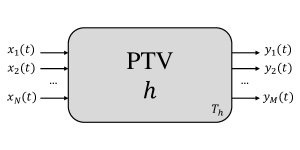
Figure 1: Representation of a generic PTV linear system, relating $N$ continuous-time inputs $x_{j}(t)$ with $M$ continuous-time outputs $y_{i}(t)$. While $h$ is the name of the PTV, $T_{h}$ stands for its period.

A clear example of PTV system is the ideal cyclical multiplexer $N:1$, shown in Fig. 2(a), a device that periodically alternates its single output between its $N$ inputs. As shown in Fig. 2(b), it can be modeled as a single-output PTV, of period $T_{h}$, given by

$$y(t)=\sum_{j=1}^{N}\int h_{j}(z_{h}(t),\tau)x_{j}(t-\tau)\,d\tau,$$ (4)

where the impulse responses are

$$h_{j}(z,\tau)=\left\{\begin{array}[]{l}\delta(\tau),\\ 0,\end{array}\right.\quad\begin{array}[]{c}(j-1)T_{h}/N\leq z<jT_{h}/N\\ \mathrm{otherwise,}\end{array}$$ (5)

being $\delta(.)$ the Dirac delta function. Another common example is the multiplier with a local oscillator input, displayed in Fig. 2(c). Although the output can be easily written as $y(t)=x(t)\mathrm{sin}(\omega_{0}t)$, we can take it to the PTV form, as shown in Fig. 2(d), by writing

$$y(t)=\int h(z_{h}(t),\tau)x(t-\tau)\,d\tau,$$ (6)

with

$$h(z,\tau)=\delta(\tau)\mathrm{sin}(\omega_{0}z)$$ (7)

and $T_{h}=2\pi/\omega_{0}$.

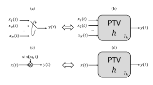
Figure 2: Examples of common PTVs: a) cyclical multiplexer $N:1$. b) equivalent $N:1$ PTV model. c) local oscillator multiplier. d) equivalent PTV model.

II Combination of PTVs

In this section we study the interaction between PTVs and time-invariant linear systems.

II-A Parallel PTVs

We consider the two PTV systems $h$ and $g$, shown in Fig. 3(a), described by the set of equations

$$y^{(h)}_{i}(t)=\sum_{j=1}^{N_{h}}\int h_{ij}(z_{h}(t),\tau)x^{(h)}_{j}(t-\tau)\,d\tau,$$ (8)

with $i\in\{1,2,...,M_{h}\}$, and

$$y^{(g)}_{i}(t)=\sum_{j=1}^{N_{g}}\int g_{ij}(z_{g}(t),\tau)x^{(g)}_{j}(t-\tau)\,d\tau,$$ (9)

with $i\in\{1,2,...,M_{g}\}$, respectively. We define a new time-variant system, $s$, whose inputs/outputs are given by

$$x_{j}(t)=\left\{\begin{array}[]{l}x^{(h)}_{j}(t),\\ x^{(g)}_{j-N_{h}},\end{array}\right.\quad\begin{array}[]{c}j\in\{1,2,..,N_{h}\}\\ j\in\{N_{h}+1,N_{h}+2,..,N_{h}+N_{g}\},\end{array}$$ (10)

and

$$y_{i}(t)=\left\{\begin{array}[]{l}y^{(h)}_{i}(t),\\ y^{(g)}_{i-M_{h}},\end{array}\right.\quad\begin{array}[]{c}i\in\{1,2,..,M_{h}\}\\ i\in\{M_{h}+1,M_{h}+2,..,M_{h}+M_{g}\}.\end{array}$$ (11)

The system $s$ is then described by the linear relationship

$$y_{i}(t)=\sum_{j=1}^{N_{s}}\int s_{ij}(t,\tau)x_{j}(t-\tau)\,d\tau\quad\forall i\in\{1,2,...,M_{s}\},$$ (12)

where $N_{s}=N_{h}+N_{g}$, $M_{s}=M_{h}+M_{g}$, and

$$s_{ij}(t,\tau)=\left\{\begin{array}[]{l}h_{ij}(z_{h}(t),\tau),\\ \qquad i\in\{1,2,...,M_{h}\}\land j\in\{1,2,...,N_{h}\}\\ g_{(i-M_{h})(j-N_{h})}(z_{g}(t),\tau),\\ \qquad i\in\{M_{h}+1,M_{h}+2,...,M_{s}\}\land\\ \qquad j\in\{N_{h}+1,N_{h}+2,...,N_{s}\}\\ 0,\quad\mathrm{otherwise.}\end{array}\right.$$ (13)

If two integers, $k_{h}$ and $k_{g}$, can be found to satisfy $k_{h}T_{h}=k_{g}T_{g}$, the system $s$ is also a PTV. The period of $s$ is given by

$$T_{s}=k_{h}T_{h}=k_{g}T_{g},$$ (14)

being $k_{h}$ and $k_{g}$ the minimum integers satisfying the equality. In other words, if $T_{s}$ exists, can be obtained as the least common multiple (lcm) of the periods $T_{h}$ and $T_{g}$. Note that $T_{s}$ exists only if $T_{h}/T_{g}$ is a rational number. The PTV behavior of $s$ can be easily proven with Eq. 13, obtaining

$$s_{ij}(t+T_{s},\tau)=s_{ij}(t,\tau)=s_{ij}(z_{s}(t),\tau).$$ (15)

Figure 3(b) shows the equivalent PTV system $s$ resulting from the parallel topology of $h$ and $g$.

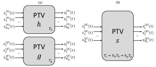
Figure 3: Parallel configuration of PTVs: a) the systems $h$ and $g$ are PTVs of period $T_{h}$ and $T_{g}$, respectively. b) equivalent PTV model $s$ of period $T_{s}$, the least common multiplier of $T_{h}$ and $T_{g}$.

II-B Series PTVs

In the series configuration of the PTVs $h$ and $g$, shown in Fig. 4(a), the $L$ outputs of system $h$ are the inputs of the system $g$. By combining the input-output equations of both systems,

$$r_{l}(t)=\sum_{j=1}^{N}\int h_{ij}(z_{h}(t),\tau)x_{j}(t-\tau)\,d\tau\quad\forall l\in\{1,2,...,L\}$$ (16)

and

$$y_{i}(t)=\sum_{l=1}^{L}\int g_{il}(z_{g}(t),\tau)r_{l}(t-\tau)\,d\tau\quad\forall i\in\{1,2,...,M\},$$ (17)

we obtain an equivalent TV linear system $s$, given by

$$y_{i}(t)=\sum_{j=1}^{N}\int s_{ij}(t,\tau)x_{j}(t-\tau)\,d\tau\quad\forall i\in\{1,2,...,M\},$$ (18)

where

$$s_{ij}(t,\tau)=\\ \sum_{l=1}^{L}\int g_{il}(\mathrm{mod}(t,T_{g}),\mu)h_{lj}(\mathrm{mod}(t-\mu,T_{h}),\tau-\mu)\,d\mu.$$ (19)

As in the case of the parallel configuration, if the lcm of both periods can be found, $s$ is proven to be a PTV system satisfying Eqs. 14 and 15. Figure 4(b) displays the equivalent PTV system of the series PTVs.

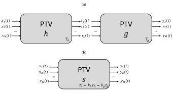
Figure 4: Series configuration of PTVs: a) the systems $h$ and $g$ are PTVs of period $T_{h}$ and $T_{g}$, respectively. b) equivalent PTV model $s$ of period $T_{s}$, the least common multiplier of $T_{h}$ and $T_{g}$.

II-C Combination with time-invariant linear systems

A time-invariant linear system can be expressed as a PTV with an arbitrary period. For instance, the linear system $L$, described by

$$y_{i}(t)=\sum_{j=1}^{N}\int L_{ij}(\tau)x_{j}(t-\tau)\,d\tau\quad\forall i\in\{1,2,...,M\},$$ (20)

can be also defined as the PTV system $h$, given by Eq. 3, where

$$h_{ij}(z_{h}(t),\tau)=L_{ij}(\tau).$$ (21)

As $h$ does not depend on $z_{h}(t)$, the period $T_{h}$ can be arbitrarily set. Consequently, combination of time-invariant linear systems with PTVs can be reduced to a unique PTV system by following the rules of parallel and series configuration introduced before.

As a simple example, we study the system shown in Fig. 5(a): a linear combination of two local oscillator multiplier lines. The blocks $A$ and $B$ represent time-invariant linear systems. In Fig. 5(b) we show the representation of all the circuit components as PTV systems. The local oscillator multipliers are converted to the systems $a$ and $b$ by following Eqs. 6 and 7, and their periods are defined as $T_{h}=2\pi/\omega_{0}$ and $T_{g}=4\pi/3\omega_{0}$, respectively. Systems $A$ and $B$ are regarded as the PTV systems $a$ and $b$ by using Eq. 21. Their periods are conveniently set to $T_{h}$ and $T_{g}$, respectively. Also, the split and sum points are regarded as 1:2 and 2:1 PTVs, respectively, both with period $T_{h}$. In the next step, shown in Fig. 5(c), we reduce the series PTVs $h$($g$) and $a$($b$) to the single PTVs $\hat{h}$($\hat{g}$). Then, as shown in Fig. 5(d), the parallel configuration of $\hat{h}$ and $\hat{g}$ is reduced to the PTV $\hat{s}$. The period $T_{s}$ can be easily calculated by expressing the period ratio as a fraction:

$$\frac{T_{h}}{T_{g}}=\frac{3}{2}\quad\Leftrightarrow\quad 2T_{h}=3T_{g}.$$ (22)

By comparing Eq. 22 with Eq. 14, we obtain $T_{s}=4\pi/\omega_{0}$. Finally, in Fig. 5(e), we reduce the serie of $c$-$\hat{s}$-$d$ in the 1:1 PTV $s$, whose period can be easily proven to be $T_{s}$.

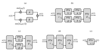
Figure 5: Example of PTV reduction: a) circuit combining PTVs (local oscillator multipliers) with time-invariant linear systems ($A$ and $B$). b) each component of the circuit is expressed in its PTV form. c) the series PTV $h$-$a$ and $g$-$b$ are reduced to the single PTV form. d) parallel reduction of the system $\hat{h}||\hat{g}$. e) final equivalent PTV system of the circuit.

III Output Bandwidth

Unlike the time-invariant linear systems, the output bandwidth of a PTV is not necessarily equal to the input bandwidth. A clear example is provided by the case shown in Fig. 2(c), where the local oscillator multiplier increases the signal bandwidth due to the frequency translation process. In this section we derive a simple formula to calculate the output bandwidth.

At the first place, we note that the frequency-domain representation of the PTV described by the impulse responses $h_{ij}(z,\tau)$ is given by the two-dimensional functions

$$\tilde{h}_{ij}(k,f)=\int_{0}^{T_{h}}\int_{-\infty}^{\infty}h_{ij}(z,\tau)e^{-\text{j}2\pi\left(kz/T_{h}+f\tau\right)}\,d\tau\,dz,$$ (23)

where $k\in\mathbb{Z}$ and $f\in\mathbb{R}$. This definition represents an hybrid transformation combining the Fourier transform on $\tau$ with the Fourier series on $z$, due to the periodic behavior of $h_{ij}$ on the last variable. The inverse of Eq. 23 leads to the definition of two bandwidths for the PTV $h$: the variation bandwidth $A_{h}$, corresponding to the discrete variable $k$, and the linear bandwidth $B_{h}$, corresponding to the continuous variable $f$, as the minimum values satisfying

$$h_{ij}(z,\tau)=\sum_{k=-A_{h}}^{A_{h}}\int_{-B_{h}}^{B_{h}}\tilde{h}_{ij}(k,f)e^{\text{j}2\pi\left(kz/T_{h}+f\tau\right)}\,d\tau$$ (24)

$\forall i,j$. While the linear bandwidth has a simple interpretation as the bandwidth of time-invariant linear systems, the variation bandwidth is a particular property of the PTVs, associated to the maximum variation speed of the impulse-response with respect to the temporal variable.

By using the definition of Eq. 23 and the inverse Fourier transform of $x_{i}$,

$$x_{i}(t)=\int_{-B_{x}}^{B_{x}}\tilde{x}_{i}(f)e^{\text{j}2\pi ft}\,df,$$ (25)

where $\tilde{x}_{i}$ and $B_{x}$ are the Fourier transform and the bandwidth of $x_{i}$, respectively, in Eq. 1 we obtain

$$y_{i}(t)=\sum_{j=1}^{N}\sum_{k=-A_{h}}^{A_{h}}\int_{-B_{x}}^{B_{x}}\int_{-B_{h}}^{B_{h}}\int\\ \tilde{h}_{ij}(k,f)\tilde{x}_{j}(f^{\prime})e^{\text{j}2\pi\left(kt/T_{h}+f\tau+f^{\prime}(t-\tau)\right)}\,d\tau\,df\,df^{\prime}.$$ (26)

By making the change of variable $f^{\prime}=\mu-k/T_{h}$ we have

$$y_{i}(t)=\sum_{k=-A_{h}}^{A_{h}}\int_{-B_{x}+k/T_{h}}^{B_{x}+k/T_{h}}\tilde{y}_{i}(k,\mu)e^{\text{j}2\pi\mu t}\,d\mu,$$ (27)

where

$$\tilde{y}_{i}(k,\mu)=\\ \sum_{j=1}^{N}\int_{-B_{h}}^{B_{h}}\int\tilde{h}_{ij}(k,f)\tilde{x}_{j}(\mu-k/T_{h})e^{\text{j}2\pi\left(f-\mu+k/T_{h}\right)\tau}\,d\tau\,df.$$ (28)

Although Eq. 27 is not an usual inverse Fourier transform, like Eq. 25, it allows for the calculation of the output bandwidth $B_{y}$, as the maximum-frequency component of $y_{i}(t)$ is clearly

$$B_{y}=B_{x}+\frac{A_{h}}{T_{h}}.$$ (29)

IV Discrete-time representation of PTVs

By knowing the output bandwidth of a PTV, we are able to perform a discrete-time representation of the system. We have to choose a sampling period $T_{\mathrm{s}}$ satisfying the Nyquist condition, i.e.

$$T_{\mathrm{s}}\leq\frac{1}{2B_{y}},$$ (30)

and then to define the discrete-time signals as

$$a[n]=a(nT_{\mathrm{s}}),$$ (31)

where $n\in\mathbb{Z}$ and $a$ stands for any input-output signal. An useful operation is the inverse of the sampling process of Eq. 31, given by

$$a(t)=\sum_{n=-\infty}^{\infty}a[n]\mathrm{sinc}\left(\frac{t}{T_{\mathrm{s}}}-n\right),$$ (32)

where $\mathrm{sinc}(x)=\mathrm{sin}(\pi x)/(\pi x)$ $\forall x\neq 0$ and $\mathrm{sinc}(0)=1$.

By using Eqs. 31 and 32 in the definition of PTV (Eq. 3), we obtain

$$y_{i}[n]=\sum_{j=1}^{N}\sum_{m=-\infty}^{\infty}H_{ij}[n,m]x_{j}[n-m],$$ (33)

where

$$H_{ij}[n,m]=\int h_{ij}(\mathrm{mod}(nT_{\mathrm{s}},T_{h}),\tau)\mathrm{sinc}\left(m-\frac{\tau}{T_{\mathrm{s}}}\right)\,d\tau.$$ (34)

Equation 33 is the definition of a discrete-time TV system, as the impulse responses $H_{ij}$ do not only depend on the input sampling index $m$ but also of the output sampling index $n$. In addition, if the sampling period is set to be a divisor of the PTV period, i.e.

$$T_{h}=K_{H}T_{\mathrm{s}}\quad K_{H}\in\mathbb{Z},$$ (35)

Eq. 33 becomes the definition of a discrete-time periodically time-variant (DTPTV) linear system, that reads

$$y_{i}[n]=\sum_{j=1}^{N}\sum_{m=-\infty}^{\infty}H_{ij}[z_{H}[n],m]x_{j}[n-m],$$ (36)

with $z_{H}[n]=\mathrm{mod}(n,K_{H})$ and being $K_{H}$ the discrete period of the system $H$. Figure 6 shows the schematic representation of a DTPTV system. Equation 36 allows for the numerical simulation of PTV system and enables the demonstration of two interesting properties, as shown in next section.

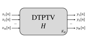
Figure 6: Representation of a generic DTPTV linear system, relating $N$ discrete-time inputs $x_{j}[n]$ with $M$ discrete-time outputs $y_{i}[n]$. While $H$ is the name of the DTPTV, $K_{H}$ stands for its discrete period.

V Inverse of PTVs

We use the discrete-time representation to prove that that the inverse of a PTV linear system, if it exists, is another PTV of the same dimension.

V-A SISO PTV

The single-input single-output PTV (SISO PTV), shown in Fig. 7(a), can be expressed in its discrete-time form as

$$y[n]=\sum_{m=-\infty}^{\infty}H[z_{H}[n],m]x[n-m]=\\ \sum_{m=-\infty}^{\infty}H[z_{H}[n],n-m]x[n].$$ (37)

An useful alternative representation of this system is given by expressing the input/output signals as vector signals of dimension $K_{H}$,

$$\left\{\begin{array}[]{l}x_{j}[r]=x[rK_{H}+j]\\ y_{i}[k]=y[kK_{H}+i],\end{array}\right.$$ (38)

where $i,j\in\{0,1,...,K_{H}-1\}$. By using the vector-signal representation of the input in Eq. 37 we obtain

$$y[n]=\sum_{j=0}^{K_{H}-1}\sum_{r=-\infty}^{\infty}H[z_{H}[n],n-rK_{H}-j]x_{j}[r].$$ (39)

Finally, by using the vector-signal representation of the output in Eq. 39 we have

$$y_{i}[k]=\sum_{j=0}^{K_{H}-1}\sum_{r=-\infty}^{\infty}\bar{H}_{i,j}[k-r]x_{j}[r],$$ (40)

where $\bar{H}$ is a $K_{H}\times K_{H}$ matrix given by

$$\bar{H}_{i,j}[n]=H[i,nK_{H}+i-j].$$ (41)

Equation 40 denotes an interesting equivalence between a SISO PTV and a time-invariant multiple-input multiple-output (MIMO) linear system, shown in Fig. 7(b). Inversely, any MIMO linear system written in the form of Eq. 40 can be represented as a SISO PTV, by defining the periodic impulse-responses as

$$H[h,m]=\bar{H}_{h,\mathrm{mod}(m,K_{H})}\left[\frac{m-\mathrm{mod}(m,K_{H})}{K_{H}}\right],$$ (42)

and the higher-rate input-output signals as

$$\left\{\begin{array}[]{l}x[n]=x_{\mathrm{mod}(n,K_{H})}\left[(n-\mathrm{mod}(n,K_{H}))/K_{H}\right]\\ y[n]=y_{\mathrm{mod}(n,K_{H})}\left[(n-\mathrm{mod}(n,K_{H}))/K_{H}\right].\end{array}\right.$$ (43)

The equivalence shown in Fig. 7 allows the simple calculation of the DTPTV inverse $H^{-1}$, as the inverse of a time-invariant MIMO $K_{H}\times K_{H}$ is another MIMO of the same dimension. Basically, the matrix representation of that inverse must satisfy

$$\sum_{j=0}^{K_{H}-1}\sum_{m=-\infty}^{\infty}\bar{H}^{(-1)}_{ij}[n]\bar{H}_{jk}[n-m]=\delta_{ik}\delta_{n0},$$ (44)

where $\delta$ stands for the Kronecker delta. In addition, by using Eqs. 42 and 43, we can write $\bar{H}^{(-1)}$ as a discrete-time SISO PTV. In conclusion, the inverse of a SISO PTV is another SISO PTV of the same period. This conclusion is also valid for continuous-time PTV systems.

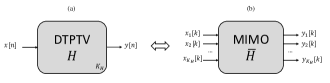
Figure 7: Equivalence between a SISO PTV and a time-invariant MIMO linear system. a) discrete-time of a SISO PTV. b) equivalent MIMO $K_{H}\times K_{H}$, obtained by considering vector signals.

V-B Square PTV

The square PTV, shown in Fig. 8(a), is defined as the PTV system whose number of inputs and number of outputs are equal ($M=N$ in definition of Eq. 3). The discrete-time representation of such system is given by

$$y_{i}[n]=\sum_{j=1}^{N}\sum_{m=-\infty}^{\infty}H_{i,j}[\mathrm{mod}(n,K_{H}),m]x_{j}[n-m],$$ (45)

where $i\in\{1,2,..,N\}$. We define a higher-rate signal to serialize the output of the system, that reads

$$y[k]=y_{i}[n],\quad\left\{\begin{array}[]{l}i=\mathrm{mod}(k,N)+1\\ n=\frac{k-\mathrm{mod}(k,N)}{N}.\end{array}\right.$$ (46)

In a similar way, we define the serialized input

$$x[k-r]=x_{j}[n-m],\quad\left\{\begin{array}[]{l}j=\mathrm{mod}(k-r,N)+1\\ m=\frac{r-\mathrm{mod}(r,N)}{N}.\end{array}\right.$$ (47)

By replacing Eqs. 46 and 47 into Eq. 45, we obtain the TV linear system

$$y[k]=\sum_{r=-\infty}^{\infty}\hat{H}[k,r]x[k-r],$$ (48)

where

$$\hat{H}[k,r]=H_{\mathrm{mod}(k,N)+1,\mathrm{mod}(k-r,N)+1}\left[\mathrm{mod}\left(\frac{k-\mathrm{mod}(k,N)}{N},K_{H}\right),\frac{r-\mathrm{mod}(r,N)}{N}\right].$$ (49)

From the definition of Eq. 49, it is easy to prove that this system is a DTPTV, since

$$\hat{H}[k+NK_{H},r]=\hat{H}[k,r].$$ (50)

Consequently, we can rewrite Eq. 48 as

$$y[k]=\sum_{r=-\infty}^{\infty}\hat{H}[z_{\hat{H}}[n],r]x[k-r],$$ (51)

where $z_{\hat{H}}[n]=\mathrm{mod}(n,K_{\hat{H}})$, being $K_{\hat{H}}=NK_{H}$.

This result means that any square DTPTV can be modeled as a higher-rate SISO DTPTV, as shown in Fig. 8(b), with a discrete period $N$ times larger. Inversely, we can prove that any SISO DTPTV $\hat{H}$, of period $K_{\hat{H}}$, can be represented as a lower-rate square DTPTV $H$ of period $K_{H}=K_{\hat{H}}/N$ by defining the parallel inputs/outputs

$$\left\{\begin{array}[]{l}x_{i}[n]=x[nN+i-1]\\ y_{i}[n]=y[nN+i-1]\end{array}\right.$$ (52)

and the periodic impulse-responses

$$H_{i,j}[n,m]=\hat{H}[nN+i-1,mN+j-1].$$ (53)

Thus, by using the equivalence of Fig. 8, we can prove that the inverse of a square DTPTV is another DTPTV, analogously to the inverse of a SISO DTPTV. Again, this conclusion is valid for continuous-time systems.

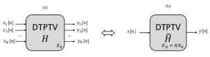
Figure 8: Equivalence between a square PTV and a SISO PTV. a) discrete-time of a square PTV. b) equivalent SISO DTPTV, with $N$ times large discrete period, obtained by considering serializing signals.

VI Conclusions

Starting from a mathematical definition of the periodically time-variant linear systems, we derived simple rules to reduce a circuit, combining different PTVs with time-invariant linear systems, to a single PTV system. By using a frequency-domain analysis of that definition, we obtained a simple formula for the output bandwidth of a PTV, enabling a suitable discrete-time representation of such systems. In addition, we also found interesting equivalences for the DTPTV systems, allowing for the derivation of a meaningful conclusion: the inverse of a square PTV is another square PTV of the same dimension.

References

- [1] Claasen, T. A. C. M. and W. Mecklenbrauker, On stationary linear time-varying systems, IEEE transactions on circuits and systems 29.3:169-184, 1982.
- [2] Middleton, Richard H. and Graham C. Goodwin, Adaptive control of time-varying linear systems, IEEE Transactions on Automatic Control 33.2:150-155, 1988.