Configurable Spatial-Temporal Hierarchical Analysis for Flexible Video Anomaly Detection

Abstract

Video anomaly detection (VAD) is a vital task with great practical applications in industrial surveillance, security system, and traffic control. Unlike previous unsupervised VAD methods that adopt a fixed structure to learn normality without considering different detection demands, we design a spatial-temporal hierarchical architecture (STHA) as a configurable architecture to flexibly detect different degrees of anomaly. The comprehensive structure of the STHA is delineated into a tripartite hierarchy, encompassing the following tiers: the stream level, the stack level, and the block level. Specifically, we design several auto-encoder-based blocks that possess varying capacities for extracting normal patterns. Then, we stack blocks according to the complexity degrees with both intra-stack and inter-stack residual links to learn hierarchical normality gradually. Considering the multisource knowledge of videos, we also model the spatial normality of video frames and temporal normality of RGB difference by designing two parallel streams consisting of stacks. Thus, STHA can provide various representation learning abilities by expanding or contracting hierarchically to detect anomalies of different degrees. Since the anomaly set is complicated and unbounded, our STHA can adjust its detection ability to adapt to the human detection demands and the complexity degree of anomaly that happened in the history of a scene. We conduct experiments on three benchmarks and perform extensive analysis, and the results demonstrate that our method performs comparablely to the state-of-the-art methods. In addition, we design a toy dataset to prove that our model can better balance the learning ability to adapt to different detection demands.

I Introduction

Video anomaly detection (VAD) is urgently needed to free manual inspection and save human resources in various emerging fields, such as traffic control, security systems, and industrial automation [1]. However, just like other outlier detection tasks, acquiring abnormal data is far more difficult than normal data. Moreover, the objective of VAD is to detect any anomaly in the real world rather than in an anomaly set preset manually, which means that we should formulate VAD as a one-class classification task [2, 3]. A well-applied solution is to determine a proper way to measure the deviations between normal and abnormal events. However, the low frequency of anomalies leads to the imbalance of normal and abnormal samples. Thus, the conventional supervised learning methods seem inappropriate [4]. With the swift development of unsupervised machine learning techniques, we can utilize proxy tasks to learn the normal patterns and detect anomaly. The key to unsupervised VAD is to learn the latent representation of the normal data distribution. Due to the significant fitting ability of deep neural networks, some deep learning-based methods are introduced to model data distribution from a vast amount of data for VAD. Among them, deep auto-encoders have been explored and show a pretty good performance. Such methods [5, 6, 7, 8] usually utilize reconstruction or prediction as proxy tasks to learn the representation of normality, which explores the corresponding loss to reveal the deviations of samples from the learned normal patterns.

Previous methods often propose a fixed structure without considering configurability [9]. Although several hand-crafted features have been proposed [10], they still lack the configurable ability to extract normal patterns to realize flexible detections. Especially, the complexity degree of anomaly and the detection demand vary from scene to scene. For example, cars can be considered abnormal objects on the sidewalk but normal ones on the driveway. The same structure means a single and restricted learning and generative ability of the model, which can not address this problem. How to make the structure of tackling VAD configurable is worth studying. Even though we can redesign these methods to adapt to different new scenes and detection demands, the detailed intra-model modifying process is quite time-consuming and complicated, like redesigning the number of convolutional layers, channels, normal patterns, and so on. Thus, we design the configurable spatial-temporal hierarchical architecture (STHA) to tackle this problem. STHA can provide various learning abilities by expanding and contracting in both vertical and horizontal directions to satisfy flexible detection demands, which will be discussed in detail in Section III.

The pattern boundary between normality and anomaly is ambiguous in flexible detection demands [11], indicating that we should balance the representation learning and generating abilities of STHA. We analyze the cause of the problem and try to solve it from the following perspectives with two concerns. (1) The representation learning ability of the auto-encoder is powerful enough to memorize the normal patterns and then reconstruct normal samples from the learned representation well. (2) The generating ability of the auto-encoder should not be too powerful to reconstruct or predict the abnormal samples well. In other words, the auto-encoder can not have the ability to imagine abnormal samples that have never been seen in the training phase. Auto-encoder and its variants are indeed powerful generative models with great imaginations used in different fields, including VAD. For instance, many methods adopt the variational auto-encoder [12, 5], denoising auto-encoder [13], and memory-augmented auto-encoder [14] to tackle VAD. Previous methods often focus on the first perspective by boosting the learning ability of the auto-encoder. In our study, we conduct experiments to prove that controlling learning and generating abilities are also meaningful.

In this paper, STHA aims to analyze anomaly hierarchically and be extendable towards making its detection goal configurable. Firstly, we design appearance and motion streams to extract the knowledge of video frames and RGB differences, respectively. Recently, multisource knowledge of VAD has been explored [15, 16]. Thus, our model can fully explore the multisource knowledge of appearance and motion information. Secondly, STHA can realize anomaly detection more accurately. On the one hand, the previous block can remove the portion of inputs that it can learn well, making the learning process of downstream blocks easier. On the other hand, a downstream block can learn a deeper representation than its previous block, which means the anomaly detected by a downstream block is more complex than its previous one. Especially, we design a feature siamese network in the block to help the reading process to better retrieve normal patterns and enhance accuracy. Thirdly, STHA can alter the tolerance degree by expanding or contracting to satisfy different detection demands. Under some conditions, we need to adjust the tolerance of anomaly in a scene. For example, a bicycle was previously forbidden to appear, but now it is allowed as long as it runs normally. Nevertheless, events like exceeding the speed limit or not driving in the specified lane are still forbidden. We can contract STHA to make adjustments without redesigning the architecture. To prove the adaptability to the detection demand of our STHA, we propose a toy dataset based on the UCSD Ped2 dataset and compare our model with state-of-the-art methods.

The contributions of this paper are as follows:

• We propose a spatial-temporal hierarchical architecture for unsupervised video anomaly detection. We formulate the memory-augmented auto-encoders as blocks and design a feature siamese network to retrieve normal patterns. We further stack these blocks to provide different learning abilities.

• The proposed STHA is configurable to adapt to various detection demands by easily expanding and contracting. We introduce a toy dataset with different tolerance degrees to prove its adaptability, which can perform a hierarchical analysis with configurable detections.

• Experimental results illustrate that our proposed STHA achieves comparable performance to the state-of-the-art methods on three benchmark datasets, indicating the proposed architecture’s effectiveness.

The rest of this paper is organized as follows. Section II introduces related work. Section III describes our proposed method, architecture, and key components in detail. Section IV describes the experiments and results. Finally, Section V summarizes and concludes.

II Related Work

The development of unsupervised VAD is becoming more and more structured. It is noted that there is rich multisource knowledge in the field of VAD. Significantly, spatial-temporal learning is now a hot topic that has been proven effective for VAD, which makes diverse methods try to explore better structures to extract different sources of knowledge along with a better way to fuse them. Thus, many methods introduced two-stream-based structures to better realize information complementarity. However, to the best of our knowledge, existing unsupervised VAD methods are not configurable enough.

II-A Spatial-Temporal Learning for VAD

Video anomaly detection is an emerging trend in studying. Since Popoola et al. [17] first introduced the reconstruction error as a loss function for visual tasks, various reconstruction-based approaches have been proposed for video anomaly detection, such as unsupervised VAD. Lu et al. [18] introduced the convolutional auto-encoder (ConvAE) to capture the spatial information of the video frames across the spatial locations. However, the approach is based on sparse coding and bag-of-words techniques to realize fast detection, which complicates the experimental settings and training process.

Hasan et al. [19] emphasized the importance of learning the temporal normality and that we should extract the temporal information of videos as sequences of frames. For temporal information significantly helps to improve the performance of VAD, plenty of methods try to explore the temporal regularities contained in the video sequences. For instance, Chong et al. [20] proposed a convolutional long short-term memory (CLSTM) based method to further enhance the preservation of temporal regularities in the training phase. The work in [21] continued the previous thinking and replaced the auto-encoders with other generative models, like energy-based models, to reconstruct patches of video frames.

Since Liu et al. [22] proposed adopting prediction as the proxy task, prediction-based methods’ performances are commonly better than reconstruction-based methods. Vu et al. [23] improved the performance of unsupervised VAD by introducing conditional generative adversarial network (GAN), which boosted the emergence of more methods that combines with GAN. Hao et al. [6] have introduced a novel approach called the spatiotemporal consistency-enhanced network (STCEN) to detect and highlight the anomalous patterns in data. STCEN addresses this problem by utilizing both spatial and temporal information in the data. Zaheer et al. [2] proposed a new approach called unsupervised Generative Cooperative Learning (GCL) to improve the performance of video anomaly detection. This method leverages the infrequent occurrence of anomalies to establish cross-supervision between a generator and a discriminator in an unsupervised setting.

II-B Two-stream Methods for VAD

Simonyan et al. [24] proposed two-stream based methods to model segments of videos and consecutive optical flow frames in the field of action recognition. Specifically, the method adopted pre-trained networks to form two streams. Network configurations in this work were set to meet different demands of two streams, such as the number of channels in the convolution layers and so on. Yan et al. [16] aimed to learn the probability distribution of appearance and motion streams by adopting recurrent variational autoencoders. It came to a conclusion that two kinds of information of appearance and motion streams are indeed mutually complementary.

For example, Liu et al. [25] first introduced margin learning techniques to learn the distributions of normality by alleviating the impact caused by the imbalanced data. Unlike other methods, the two streams of this work were to model normal and abnormal videos, respectively. Nguyen et al. [26] proposed to link the object appearances in the common frames with its motions by utilizing deep convolutional neural networks. It aimed to correlate the normal motion characteristics to appearance structures. In the testing phase, the unlearned correlations of appearance and motion were therefore detected as anomalies.

Xu et al. [13] first adopted two stacked denoising auto-encoders to learn the appearance and motion representations from video frames and corresponding optical flows between consecutive frames. Then the method further adopted a third denoising auto-encoder to learn the joint representation of spatial-temporal information. By exploring the relationship between appearance and motion representation, it aims to find a way to recruit the reciprocal forces of two types of representation. At last, it fed the appearance, motion, and joint representation into three one-class support vector machines (SVMs) as downstream classifiers. It also fused the outputs of three SVMs to complete the detection. Enlighted by the method, more two-stream based approaches are introduced and modified to address VAD by exploring the consistency of motion and appearance. Cai et al. [4] proposed an appearance-motion memory consistency network to model the correlations of two streams. This work proved that memory modules combined with two-stream structures could significantly improve the memorizing and predicting abilities of networks in the high dimensional spaces.

III Methods

III-A Overall Architecture

To use symbols correctly and clearly in the following paragraphs, we first introduce the data organization in this work. We adopt a sliding window to capture sequences of $K$ consecutive frames from video frames $\bm{X}_{n}^{f}\in\mathbb{R}^{H\times W}$ and denote each sequence as a sample, represented as $\bm{x}_{t}^{f}=\left\{\bm{X}_{n}^{f}\right\}_{n=1}^{K}$, where $H$ and $W$ are the height and width of a frame, respectively. Thus, we can further denote a video as $\mathcal{V}=\left\{\bm{x}_{t}^{f}\right\}_{t=1}^{N-K+1}$, where $N$ is the frame length of a video and $t$ is the index of the sample. For RGB difference $\bm{X}_{n}^{d}\in\mathbb{R}^{H\times W}$, we formulate the dataset just like video frames. Samples are denoted as $\bm{x}_{t}^{d}=\left\{\bm{X}_{n}^{d}\right\}_{n=1}^{\tilde{K}}$. Each sample contains $\tilde{K}$ consecutive RGB difference frames. The RGB difference dataset is denoted as $\mathcal{D}=\left\{\bm{x}_{t}^{d}\right\}_{t=1}^{\tilde{N}-\tilde{K}+1}$. We denote the input of a stream and the $l$-th block as $\bm{x}_{t}$ and $\bm{x}_{t,l}$, respectively. The input of the first block $\bm{x}_{t,1}$ is exactly the stream input $\bm{x}_{t}$. Furthermore, $\hat{\bm{x}}_{t,l}$ and $\hat{\bm{Y}}_{t,l}$ are the reconstructed input and block prediction of the $l$-th block.

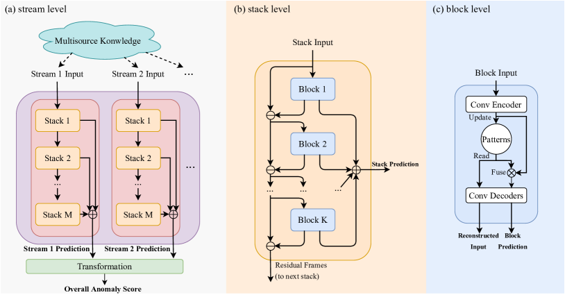
Figure 1: Illustration of the proposed spatial-temporal hierarchical analysis (STHA). After the analysis of the input of a block $\bm{x}_{t,l}$, it outputs the residual results as the input of the next block $\bm{x}_{t,l+1}$ through decomposing residual connections. The rest of the stacks and blocks carry out the same operations sequentially. The predictions of blocks $\hat{\bm{Y}}_{t,l}$ are first integrated into a stack prediction $\hat{\bm{Y}}_{t,i}$ at the stack level through the integrating residual connections. Then the stack predictions $\hat{\bm{Y}}_{t,i}$ are added as a stream prediction $\hat{\bm{Y}}_{t}$. These stream predictions are finally fused to obtain the overall anomaly score through a transformation.

As shown in Fig. 1, our proposed STHA can be delineated into a tripartite hierarchy: the stream, stack, and block levels. The block is considered the basic component. STHA utilizes the double-nested residual connections (DNRC) to combine blocks into a stack. Blocks in a stack share the same structure. Then the stream is composed of multiple stacks using DNRC. The DNRC helps the architecture to be deeper and more hierarchical. Firstly, a block adds its input $\bm{x}_{t,l}$ to its reconstructed input $\hat{\bm{x}}_{t,l}$ as the residual result $\bm{x}_{t,l+1}$, which is fed into the next block [27]. We call this operation decomposing residual connections. The following equation can describe it:

$$\bm{x}_{t,l+1}=\bm{x}_{t,l}-\hat{\bm{x}}_{t,l}.$$ (1)

In this work, the purpose of decomposing residual connections lies in that the previous block can remove the portion of inputs that it can learn well, making the learning process of downstream blocks easier. Moreover, a downstream block can learn deeper representation than its previous block, enabling it to detect some more complex anomaly. Thus, the normal patterns can be learned better by decomposing them into different levels. Secondly, all block predictions $\hat{\bm{Y}}_{t,l}$ in one stack are added to be the stack prediction $\hat{\bm{Y}}_{t,i}$. All stack predictions $\hat{\bm{Y}}_{t,i}$ in one stream are further added to be the stream prediction $\hat{\bm{Y}}_{t}$. We call this operation integrating residual connections. It can be described by the following equations:

$$\hat{\bm{Y}}_{t}=\sum_{i}\hat{\bm{Y}}_{t,i},$$ (2)

$$\hat{\bm{Y}}_{t,i}=\sum_{l}\hat{\bm{Y}}_{t,l}.$$ (3)

Combining the decomposing and integrating residual connections, namely the DNRC, the extracted information can flow and be aggregated hierarchically.

Typically, a single simple model can only learn a simple distribution, which could result in some complex anomalies being missed in the detection. However, a single complex model is likely to learn a too complex distribution, which could result in samples slightly different from the training set being mistaken as anomalies for overfitting. The performance of such models is highly dependent on the hand-crafted structures. Our proposed STHA can significantly ameliorate this issue by making full use of organizing multiple blocks hierarchically. The reason for designing the stack level lies in that a set of blocks, namely one stack, can only represent fixed extracted information. We need to apply several sets of blocks to make human interpretable detections in different detection demands. We often expand or contract several consecutive blocks to alter the learning ability. Thus, we combine these blocks into stacks to assemble different learning abilities and further expand and contract at the stack level. STHA can be altered according to the tolerance degree by masking stacks. Each stream processes one kind of knowledge individually to output the stream prediction. We attempt to exploit the multisource knowledge extracted from different streams implicitly. We apply a transformation to fuse the information and enhance the performance of VAD.

III-B Architecture of Blocks

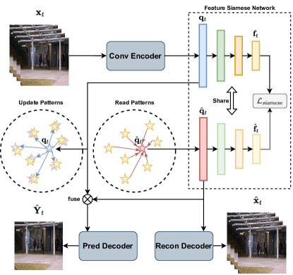
Figure 2: Overview of the architecture of a block. The convolutional encoder, predicting decoder, and reconstructing decoder are abbreviated as conv encoder, pred decoder, and recon decoder in the figure. The encoder inputs $\bm{x}_{t,l}$ and outputs the query set $\bm{q}_{t}\in\mathbb{R}^{M\times C}$. In the reading phase, we calculate the attention scores $a_{t}^{m,n}$ between queries and all normal patterns to obtain $\hat{\bm{q}}_{t}$. The reconstructing decoder inputs the reconstructed query set $\bm{q}_{t}$ and outputs the reconstructed inputs. The predicting decoder inputs the fusion of $\bm{q}_{t}$ and $\hat{\bm{q}}_{t}$ to generate the block prediction.

As shown in Fig. 2, our block is primarily comprised of five constituent components: the convolutional encoder, predicting decoder, reconstructing decoder, feature siamese network, and normal patterns. The encoder and decoders are uniquely designed based on the U-Net architecture [28]. The U-Net architecture is commonly employed for extracting latent representations from the input via dimension reduction, as well as for reconstructing the input from the latent representations through dimension increase.

Firstly, the block outputs both the block prediction and reconstructed inputs. The block prediction is integrated at the stack level as a crucial element to aid in VAD. The reconstructed inputs represent the information that the current block has learned and are utilized for calculating the residual frames at the inter-block level. The residual frames are the remaining portions that previous blocks have not learned well and can help to guide the downstream blocks to learn deeper representations. Thus, we design two parallel decoders to reconstruct the input frames and predict the future frame from the same latent representations extracted by the encoder. We only need to utilize the block prediction to calculate losses and train our model. The reason is that the residual frames of each block are computed using the reconstructed input of the preceding block’s reconstructing decoder, enabling effective training of the reconstructing decoder network. To ensure that the reconstructed inputs represent the current block’s learned portion better, we abandon the skip connection for the reconstructing decoder while maintaining it for the predicting decoder. The reconstructing decoder is prohibited from learning to copy the inputs through skip connections.

Secondly, we design a feature siamese network to make the extracted query set $\bm{q}_{t}$ of normal samples easier to reconstruct using the learned patterns. The siamese network is a one-shot learning structure for evaluating the similarity of the two inputs, which is widely used in computer visions [29, 30]. For our method adopts the prediction task as the proxy task to learn the normal patterns, we need to ensure that the learned patterns accurately represent the normality and that the reconstructed query has only normal characteristics. Specifically, normal patterns are intended to accurately reconstruct queries from normal samples while producing poor reconstructions for queries from abnormal samples. Since the training set is comprised of normal samples, we are unable to identify whether the queries from abnormal samples are poorly reconstructed in the training phase. So, we need to control the generalization ability of patterns. It is noted that the extracted queries of normal samples can not be hard for normal patterns to reconstruct. In this case, the patterns will intend to become powerful in generalizing and result in successfully predicting abnormal samples. We need to ensure that the extracted queries are easy for normal patterns to reconstruct so that the patterns can focus more on preserving normal representations rather than becoming stronger to generalize. The feature siamese network imposes restrictions to explore patterns that facilitate easier reconstruction of the query in the feasible solution domain.

The encoder inputs $\bm{x}_{t,l}$ and outputs the query set $\bm{q}_{t}\in\mathbb{R}^{M\times C}$, where $M$ is the number of queries and $C$ is the number of channels. We denote $\bm{q}_{t}^{m}\in\mathbb{R}^{C}$ as individual queries in the query set, where $m=1,\ldots,M$. Firstly, we utilize the query set to read the normal patterns and reconstruct $\hat{\bm{q}}_{t}$. We feed $\bm{q}_{t}$ and $\hat{\bm{q}}_{t}$ into the feature siamese network to calculate their similarity as a portion of training loss. Then we update the normal patterns to memorize latent representations of normality. The reconstructing decoder inputs the reconstructed query set $\bm{q}_{t}$ and outputs the reconstructed inputs. The predicting decoder inputs the fusion of $\bm{q}_{t}$ and $\hat{\bm{q}}_{t}$ to generate the block prediction.

The normal patterns consist of $N$ latent vectors that implicitly represent the normality distribution. We denote the vectors as $\bm{k}_{t}^{n}\in\mathbb{R}^{C}$, where $n=1,\ldots,N$. In the reading phase, we first compute the attention scores between $\bm{q}_{t}^{m}$ and all normal patterns as follows:

$$a_{t}^{m,n}=\frac{\frac{1}{1+\left\|\left(\bm{q}_{t}^{m}\right)^{\mathrm{T}}\bm{k}_{t}^{n}\right\|}}{\sum\limits_{i=1}^{N}\frac{1}{1+\left\|\left(\bm{q}_{t}^{m}\right)^{\mathrm{T}}\bm{k}_{t}^{i}\right\|}}.$$ (4)

We apply the t-distributed-based normalization to make it more sparse when reading normal patterns. It can make the attention scores between dissimilar $\bm{q}_{t}^{m}$ and $\bm{k}_{t}^{n}$ smaller without affecting the attention scores between similar ones being large. For each query $\bm{q}_{t}^{m}$, we apply a weighted average of all patterns $\bm{k}_{t}^{n}$ with corresponding attention scores $a_{t}^{m,n}$ to reconstruct $\hat{\bm{q}}_{t}$ as follows:

$$\hat{\bm{q}}_{t}^{m}=\sum_{i}^{N}a_{t}^{m,i}\cdot\bm{k}_{t}^{i}.$$ (5)

Then we apply the same operations to all queries and obtain the corresponding reconstructed queries $\quad\hat{\bm{q}}_{t}=\left\{\hat{\bm{q}}_{t}^{1},\ldots,\hat{\bm{q}}_{t}^{N}\right\}$.

In the updating phase, we first compute the attention scores between $\bm{k}_{t}^{n}$ and all queries as follows:

$$b_{t}^{m,n}=\frac{\frac{1}{1+\left\|\left(\bm{q}_{t}^{m}\right)^{\mathrm{T}}\bm{k}_{t}^{n}\right\|}}{\sum\limits_{j=1}^{M}\frac{1}{1+\left\|\left(\bm{q}_{t}^{j}\right)^{\mathrm{T}}\bm{k}_{t}^{n}\right\|}}.$$ (6)

For each pattern $\bm{k}_{t}^{n}$, we apply a weighted average of all queries with corresponding attention scores $b_{t}^{m,n}$ to update $\bm{k}_{t+1}^{n}$ as follows:

$$\bm{k}_{t+1}^{n}=\sigma\left(\bm{k}_{t}^{n}+\sum_{j}^{M}b_{t}^{j,n}\cdot\bm{q}_{t}^{j}\right),$$ (7)

where $\sigma$ is the logistic sigmoid function.

III-C Training Loss and Abnormality Score

Since adopting predicting future frames as the proxy task to detect the anomaly, we design several appropriate losses to train our model better. Generally, we use the prediction, pattern diversity, and feature siamese losses to formulate the overall loss as follows:

$$\mathcal{L}=\mathcal{L}_{pred}+\lambda_{d}\mathcal{L}_{diversity}+\lambda_{s}\mathcal{L}_{siamese},$$ (8)

where $\mathcal{L}_{pred}$, $\mathcal{L}_{diversity}$, and $\mathcal{L}_{siamese}$ are the prediction, pattern diversity, and the feature siamese losses, respectively. The hyperparameters $\lambda_{d}$ and $\lambda_{s}$ are used to balance different losses. Video frames and RGB difference are both suitable for measuring the intensity difference. Thus, we calculate the L2 distance between the predicted frame $\hat{\bm{Y}}_{t}$ and ground truth $\bm{Y}_{t}$ to obtain the prediction loss as follows:

$$\mathcal{L}_{pred}=\sum_{t}^{T}\left\|\hat{\bm{Y}}_{t}-\bm{Y}_{t}\right\|_{2},$$ (9)

where $T$ represents the number of samples.

Normal patterns of different blocks should be diverse to learn hierarchical levels of normality. To restrict blocks to learn distinct latent representations, we design the pattern diversity loss as follows:

$$\mathcal{L}_{diversity}=\frac{1}{N^{\prime}}\sum_{\bm{k}_{t}^{n^{\prime}}\in\bm{U}_{ab}}\sum_{\bm{k}_{t}^{i}\in\bm{U}_{ob}}\left\|\bm{k}_{t}^{n^{\prime}}-\bm{k}_{t}^{i}\right\|_{2},$$ (10)

where $\bm{U}_{ob}$ represents the set of all patterns not in the same block, $N^{\prime}$ represents the total number of all patterns, and $\bm{U}_{ab}$ represents the set of patterns in all blocks. The pattern diversity loss ensures that different blocks can learn and store distinct normality.

The siamese networks share the same parameters. As a one-shot learning method, the feature siamese network inputs the $\bm{q}_{t}$ and $\hat{\bm{q}}_{t}$ simultaneously. Then it computes the cosine similarity of embeddings $\bm{f}_{t}$ and $\hat{\bm{f}}_{t}$, and obtain the similarity score as follows:

$$\bm{f}_{t} =f\left(\bm{q}_{t}\right),$$ (11)

$$\hat{\bm{f}}_{t} =f\left(\hat{\bm{q}}_{t}\right),$$ (12)

$$\mathcal{S}_{cosine} =\frac{\bm{f}_{t}\cdot\hat{\bm{f}}_{t}}{\left\|\bm{f}_{t}\right\|\|\hat{\bm{f}}_{t}\|},$$ (13)

where $f(\cdot)$ denotes the embedding function of siamese networks.

If the similarity score is high, it represents that $\bm{q}_{t}$ can be easily reconstructed by normal patterns to be $\hat{\bm{q}}_{t}$. Thus, the feature siamese loss is defined as follows:

$$\mathcal{L}_{siamese}=-\mathcal{S}_{cosine}.$$ (14)

In the training phase, we manage to train our model to make the extracted queries of anomaly unable to be reconstructed well by normal patterns. In the testing phase, we need to exploit it to measure the deviation between the testing sample and learned normality. We compute the PSNR between the prediction and its ground truth as follows:

$$\mathcal{S}_{ano}=g\left(10\log_{10}\frac{P\cdot\max\left(\hat{\bm{Y}}_{t}\right)}{\left\|\hat{\bm{Y}}_{t}-\bm{Y}_{t}\right\|_{2}^{2}}\right),$$ (15)

where $P$ denotes the number of pixels in the video frame or RGB difference, and $g(\cdot)$ denotes the normalization function.

IV Results

IV-A Comparison with State-of-the-art Methods

TABLE I: Comparison of implementation details of STHA experiments on three benchmarks. Notes: Block-s, Block-m, Block-l, and Total Patterns in the top row represent the number of them in different models.

Dataset	Block-s	Block-m	Block-l	Total Patterns
UCSD Ped2	2	0	0	100
CUHK Avenue	1	2	0	150
ShanghaiTech	0	1	2	250

To prove the predicting accuracy of our proposed STHA, we conduct experiments with the frame-level area under the curve (AUC) as our evaluation metric on three benchmarks: the UCSD Ped2 [31], CUHK Avenue [18], and ShanghaiTech [21] datasets. Besides, the UCSD Ped1 dataset is used to select the hyperparameters. We design three types of blocks called Block-s, Block-m, and Block-l, respectively. The Block-s is the smallest block with 6 hidden layers and 50 patterns. The Block-m is the medium block with 12 hidden layers and 50 patterns. The Block-l is the largest block with 18 hidden layers and 100 patterns. As stated in Section 1, expanding and contracting at the stack level are designed to satisfy different detection demands. For the demand here is determined to detect any anomaly in a scene, we design the models of three benchmarks to have only one stack but different blocks. The STHA settings for three benchmarks are shown in Table I.

We set the training batch size to 8. We also use the Adam optimizer with an initial learning rate of 0.0001. The ReLU and sigmoid activations help the gradients flow better. We utilized the grid search on UCSD Ped1 to determine the hyperparameters: $\lambda_{d}=0.13$ and $\lambda_{s}=0.28$.

TABLE II: Results of frame-level AUC comparisons on three benchmarks. Notes: Bolded numbers indicate the best performance.

Type & Structure		Methods	UCSD Ped2	CUHK Avenue	ShanghaiTech
Traditional manual feature-based		MPPCA [32]	69.3	-	-
		MPPC+SFA [32]	61.3	-	-
		MDT [33]	82.9	-	-
Deep learning-based	Single-stream	ConvLSTM-AE [34]	88.1%	77.0%	-
		AE-Conv3D [35]	91.2%	77.1%	-
		Stacked RNN [36]	92.2%	81.7%	68.0%
		AnomalyNet [37]	94.9%	86.1%	-
		Autoregressive [38]	95.4%	-	72.5%
		MemAE [14]	94.1%	83.3%	71.2%
		DDGAN [39]	94.9%	85.6%	73.7%
		STCEN [6]	96.9%	86.6%	73.8%
	Multi-stream	AMDN [13]	90.8%	-	-
		AbnormalGAN [20]	93.5%	-	-
		FFP [22]	95.4%	85.1%	72.8%
		LIF [40]	96.5%	86.0%	73.3%
		AMMC-Net [4]	96.6%	86.6%	73.7%
		STC-Net [41]	96.7%	87.8%	73.1%
		Chang et al. [7]	96.7%	87.1%	73.7%
		BiP [42]	97.4%	86.7%	73.6%
		STHA (ours)	98.0%	88.9%	74.0%

As shown in Table II, we compare our proposed STHA with previous methods on three benchmarks. For STHA can provide various representation learning abilities by expanding or contracting hierarchically, it performs comparably with the state-of-the-art methods on three benchmarks. Compared with the previous methods, our STHA method is 0.6%, 1.1%, and 0.2% higher than SOTAs on UCSD ped2, CUHK Avenue, and ShanghaiTech datasets, respectively. The results show that our STHA method can better exploit the normality hierarchically. The same structure of previous methods leads to a restricted learning ability of the model. The adjustments of their learning abilities are often complex. The detailed intra-model modifying process is quite trifling, and the results vary greatly due to different network designs. However, STHA is more stable and able to adapt to different detection demands by simply expanding or contracting.

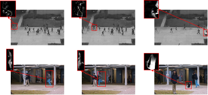
Figure 3: Illustration of the visual difference of the predicted frames and ground truth. The red window indicates anomalies.

Fig. 3 shows the visual difference between the predicted frames and ground truth of abnormal events, where the red window indicates anomalies. For STHA adopts the prediction task as its proxy task, making the predicted results of abnormal samples significantly differ from the ground truth. Fig. 3 first shows that our STHA can realize effective VAD by analyzing the difference between predicted results and ground truth when abnormal events happen as the foundation. It further reveals that the learning and generative ability of the detecting model should be controlled to avoid missing the anomaly caused by the powerful generative ability of the model. Our STHA can better model the normality and make the predicted results different from the ground truth of anomalies by utilizing the learned patterns.

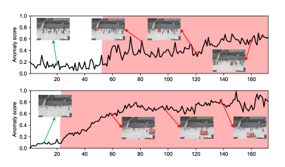
Figure 4: Illustration of temporal localization results of the detection.

Fig. 4 further shows the temporal results of the detection, where the red areas indicate abnormal. The experiments are conducted on the UCSD Ped2 dataset. The anomaly score can quickly and accurately reveal the occurrence of anomalous events, demonstrating the ability and significant potential of the proposed STHA model. Furthermore, the rapid and precise changes in the anomaly score provide valuable insights into the temporal dynamics of abnormal events, enabling efficient detection and diagnosis of such events.

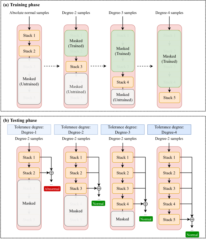
Figure 5: Flexible detections of STHA of different anomaly degree demands. We show the training (a) and testing (b) settings of STHA performing flexible detections under different circumstances of tolerance degrees.

IV-B Experiments of Flexible Detections

TABLE III: Performance on the toy dataset in three differenet tolerance degrees.

Tolerance Degree	Satck-1	Satck-2	Satck-3	Performance
Degree-1	✓			98.0%
Degree-2	✓	✓		98.2%
Degree-3	✓		✓	97.9%

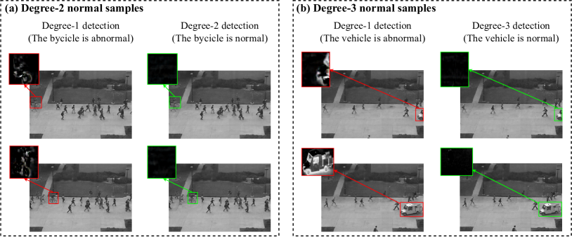
Figure 6: Visualization results of flexible detections. We show the detection results of Degree-2 (a) and Degree-3 (b) normal samples in different detection demands.

The definition of anomaly is ambiguous and varies under different circumstances. Sometimes, we demand to control and change the tolerance when detecting the anomaly. For example, the traffic rules of some lanes are flexible due to the morning and evening rush hours. To this end, we can utilize STHA to tackle this problem without designing several different models to adapt to different detection demands. We define the anomaly that needed to be flexibly detected as the flexible anomaly and manually set the tolerance degree of the flexible anomaly. As shown in Fig. 5 (a), STHA leverages its structural advantages to learn and detect hierarchically. In the training phase, we first mask the downstream stacks (stack 3 to 5 in Fig. 5 (a)) of STHA and feed the absolute normal samples to train the remaining stacks (stack 1 and stack 2 in Fig. 5 (a)). Thus, the trained stacks can detect any anomaly and represent the lowest tolerance degree: Degree-1. Then, we mask the trained stacks and unmask the downstream stack (stack 3 in Fig. 5 (a)). We input the training samples of the higher tolerance degree (Degree-2 samples in Fig. 5 (a)) to train stack 3. Thus, stack 3 learns and stores the normality of Degree-2 samples. We further unmask more downstream stacks and feed them training samples of higher tolerance to enable STHA to detect the anomaly of more tolerance degrees flexibly. As shown in Fig. 5 (b), we can set the tolerance degree to Degree-1. In this case, the STHA only activates stack 1 and stack 2. For stack 1 and stack 2 only store the normality of the absolute normal samples, Degree-2 samples are detected as anomalies in the demand for the lowest tolerance degree. While we set the tolerance degree to be Degree-2, the STHA activates stack1 to stack 3. For stack 3 stores the normality of Degree-2 samples, they are detected as normal samples.

To prove the flexibility of our STHA, we design a toy dataset based on the UCSD ped2 dataset. The anomaly of the UCSD ped2 dataset is mainly composed of the emergence of bikes and vehicles. Thus, we set three tolerance degrees: Degree-1, Degree-2, and Degree-3. Degree-1 is the lowest degree. In this case, we do not allow bikes and vehicles to appear. Degree-2 allows the bikes to appear while the vehicles are prohibited. Degree-3 further allows vehicles to appear, but bikes are not allowed to appear. We reorgnize the UCSD ped2 dataset following the next steps. Firstly, we sample some video frames that have bikes and add them into the training set as the Degree-2 normal samples. Secondly, we sample some video frames that have vehicles and add them into the training set as the Degree-3 normal samples. On the top of the trained model for the UCSD ped2, we add two downstream stacks and define the three stacks as Stack-1 to 3 from top to bottom. Thirdly, as stated in the Section 3, we mask other stacks and input the Degree-2 normal samples to train Stack-2. Similarly, we train Stack-3 with Degree-3 normal samples. In the training phase, samples that have bikes are considered abnormal in Degree-1 and Degree-3 but normal in Degree-2. Samples that have vehicles are considered abnormal in Degree-1 and Degree-2 but normal in Degree-3. Samples that have both bikes and vehicles are always considered abnormal. The performances of three degrees are shown in Table III.

Table III indicates that STHA can hierarchically store the normality of different levels in different stacks without redesigning or training a new model from scratch. STHA first learns the normal patterns of samples with no bikes or vehicles. Then the added downstream stacks further learn the patterns of bikes and vehicles, allowing STHA to realize flexible detections. Thus, STHA can provide various representation learning abilities by expanding or contracting hierarchically to detect anomalies of different degrees. As shown in Fig. 6, the visualization results prove the effectiveness of flexible detections. Degree-2 normal samples should be detected as abnormal and normal in the demand of Degree-1 and Degree-2, respectively. Thus, we conduct Degree-1 and Degree-2 detections on the Degree-2 normal samples as shown in Fig. 6 (a). Similarly, we also conduct Degree-1 and Degree-3 detections on the Degree-3 normal samples as shown in Fig. 6 (b). The red windows indicate the samples being detected as abnormal, while the green windows indicate normal, verifying configurable representation learning abilities and the capacity of accurate flexible detections.

IV-C Ablation Study

TABLE IV: Results of ablation study.

Model	Feature siamese network	Normal patterns	$\mathcal{L}_{diversity}$	Performance
1		✓	✓	96.30%
2	✓		✓	95.20%
3	✓	✓		95.90%
4	✓	✓	✓	98.00%

Table IV shows the results of the ablation analysis on key components and the loss of STHA. We conduct experiments on the UCSD ped2 dataset without feature siamese network, normal patterns, and $\mathcal{L}_{diversity}$ to verify their importance. The performance of Model 1 indicates that it will lose the partial capacity for better modeling the normal patterns without feature siamese network, meaning the performance drops by $1.7\%$. The performance of Model 2 without normal patterns drops by $2.8\%$. This is because it is so generative that it can reconstruct some abnormal samples and miss detecting some anomalies, proving that normal patterns are key modules of controlling the generative ability of the model. Model 3 without $\mathcal{L}_{diversity}$ will make normal patterns of different stacks close to each other and lead to suboptimal results, which means the performance drops by $2.1\%$.

V Conclusion

In this paper, we propose a configurable architecture called STHA to realize flexible video anomaly detection by modeling the normality hierarchically. To control the generalizing ability of basic blocks, we propose the feature siamese network to help normal patterns focus more on preserving normal representations rather than becoming stronger to generalize. To integrate hierarchical information and provide various learning abilities, we design the STHA to be structurally configurable by utilizing the double-nested residual connections to organize the blocks sequentially. Further, we explore the multisource knowledge by designing two parallel streams consisting of stacks. Thus, STHA is configurable enough to provide various representation learning abilities by expanding or contracting hierarchically and performs comparably with the SOTAs on three benchmarks. Unlike some methods that have fixed model structures, our STHA can easily alter to satisfy different detection demands in a modular manner. To prove the flexible detection ability of STHA, we design a toy dataset and conduct experiments on it. The experimental results show that our proposed STHA can realize accurate VAD in different anomaly degrees without redesigning or training the model from scratch.

References

- [1] Y. Liu, D. Yang, Y. Wang, J. Liu, and L. Song, “Generalized video anomaly event detection: Systematic taxonomy and comparison of deep models,” arXiv preprint arXiv:2302.05087, 2023.
- [2] M. Z. Zaheer, A. Mahmood, M. H. Khan, M. Segu, F. Yu, and S.-I. Lee, “Generative cooperative learning for unsupervised video anomaly detection,” in IEEE Conference on Computer Vision and Pattern Recognition, 2022, pp. 14 744–14 754.
- [3] X. Zhang, J. Fang, B. Yang, S. Chen, and B. Li, “Hybrid attention and motion constraint for anomaly detection in crowded scenes,” IEEE Transactions on Circuits and Systems for Video Technology, vol. 33, no. 5, pp. 2259–2274, 2022.
- [4] R. Cai, H. Zhang, W. Liu, S. Gao, and Z. Hao, “Appearance-motion memory consistency network for video anomaly detection,” in Proceedings of the AAAI Conference on Artificial Intelligence, 2021, pp. 938–946.
- [5] G. Slavic, D. Campo, M. Baydoun, P. Marin, D. Martín, L. Marcenaro, and C. S. Regazzoni, “Anomaly detection in video data based on probabilistic latent space models,” in IEEE Conference on Evolving and Adaptive Intelligent Systems, 2020, pp. 1–8.
- [6] Y. Hao, J. Li, N. Wang, X. Wang, and X. Gao, “Spatiotemporal consistency-enhanced network for video anomaly detection,” Pattern Recognition, vol. 121, p. 108232, 2022.
- [7] Y. Chang, Z. Tu, W. Xie, B. Luo, S. Zhang, H. Sui, and J. Yuan, “Video anomaly detection with spatio-temporal dissociation,” Pattern Recognition, vol. 122, p. 108213, 2022.
- [8] P. Xing and Z. Li, “Visual anomaly detection via partition memory bank module and error estimation,” IEEE Transactions on Circuits and Systems for Video Technology, 2023.
- [9] Y. Liu, J. Liu, M. Zhao, D. Yang, X. Zhu, and L. Song, “Learning appearance-motion normality for video anomaly detection,” in IEEE International Conference on Multimedia and Expo, 2022, pp. 1–6.
- [10] K. Deepak, G. Srivathsan, S. Roshan, and S. Chandrakala, “Deep multi-view representation learning for video anomaly detection using spatiotemporal autoencoders,” Circuits, Systems, and Signal Processing, vol. 40, pp. 1333–1349, 2021.
- [11] M. Z. Zaheer, J. Lee, M. Astrid, and S. Lee, “Old is gold: Redefining the adversarially learned one-class classifier training paradigm,” in IEEE Conference on Computer Vision and Pattern Recognition, 2020, pp. 14 171–14 181.
- [12] Y. Fan, G. Wen, D. Li, S. Qiu, M. D. Levine, and F. Xiao, “Video anomaly detection and localization via gaussian mixture fully convolutional variational autoencoder,” Computer Vision and Image Understanding, vol. 195, p. 102920, 2020.
- [13] D. Xu, Y. Yan, E. Ricci, and N. Sebe, “Detecting anomalous events in videos by learning deep representations of appearance and motion,” Computer Vision and Image Understanding, vol. 156, pp. 117–127, 2017.
- [14] D. Gong, L. Liu, V. Le, B. Saha, M. R. Mansour, S. Venkatesh, and A. v. d. Hengel, “Memorizing normality to detect anomaly: Memory-augmented deep autoencoder for unsupervised anomaly detection,” in IEEE Conference on Computer Vision and Pattern Recognition, 2019, pp. 1705–1714.
- [15] N. Li and F. Chang, “Video anomaly detection and localization via multivariate gaussian fully convolution adversarial autoencoder,” Neurocomputing, vol. 369, pp. 92–105, 2019.
- [16] S. Yan, J. S. Smith, W. Lu, and B. Zhang, “Abnormal event detection from videos using a two-stream recurrent variational autoencoder,” IEEE Transactions on Cognitive and Developmental Systems, vol. 12, no. 1, pp. 30–42, 2018.
- [17] O. P. Popoola and K. Wang, “Video-based abnormal human behavior recognition—a review,” IEEE Transactions on Systems, Man, and Cybernetics, Part C (Applications and Reviews), vol. 42, no. 6, pp. 865–878, 2012.
- [18] C. Lu, J. Shi, and J. Jia, “Abnormal event detection at 150 FPS in MATLAB,” in IEEE International Conference on Computer Vision, 2013, pp. 2720–2727.
- [19] M. Hasan, J. Choi, J. Neumann, A. K. Roy-Chowdhury, and L. S. Davis, “Learning temporal regularity in video sequences,” in IEEE Conference on Computer Vision and Pattern Recognition, 2016, pp. 733–742.
- [20] M. Ravanbakhsh, M. Nabi, E. Sangineto, L. Marcenaro, C. Regazzoni, and N. Sebe, “Abnormal event detection in videos using generative adversarial nets,” in IEEE International Conference on Image Processing, 2017, pp. 1577–1581.
- [21] H. Vu, D. Phung, T. D. Nguyen, A. Trevors, and S. Venkatesh, “Energy-based models for video anomaly detection,” arXiv preprint arXiv:1708.05211, 2017.
- [22] W. Liu, W. Luo, D. Lian, and S. Gao, “Future frame prediction for anomaly detection–a new baseline,” in IEEE Conference on Computer Vision and Pattern Recognition, 2018, pp. 6536–6545.
- [23] H. Vu, T. D. Nguyen, T. Le, W. Luo, and D. Q. Phung, “Robust anomaly detection in videos using multilevel representations,” in Proceedings of the AAAI Conference on Artificial Intelligence, 2019, pp. 5216–5223.
- [24] A. Sarabu and A. K. Santra, “Distinct two-stream convolutional networks for human action recognition in videos using segment-based temporal modeling,” Data, vol. 5, no. 4, p. 104, 2020.
- [25] W. Liu, W. Luo, Z. Li, P. Zhao, and S. Gao, “Margin learning embedded prediction for video anomaly detection with A few anomalies,” in International Joint Conference on Artificial Intelligence, 2019, pp. 3023–3030.
- [26] T. Nguyen and J. Meunier, “Anomaly detection in video sequence with appearance-motion correspondence,” in IEEE International Conference on Computer Vision, 2019, pp. 1273–1283.
- [27] K. He, X. Zhang, S. Ren, and J. Sun, “Deep residual learning for image recognition,” in IEEE Conference on Computer Vision and Pattern Recognition, 2016, pp. 770–778.
- [28] O. Ronneberger, P. Fischer, and T. Brox, “U-net: Convolutional networks for biomedical image segmentation,” in Medical Image Computing and Computer-Assisted Intervention. Springer, 2015, pp. 234–241.
- [29] S. Zagoruyko and N. Komodakis, “Learning to compare image patches via convolutional neural networks,” in IEEE Conference on Computer Vision and Pattern Recognition, 2015, pp. 4353–4361.
- [30] L. Bertinetto, J. Valmadre, J. F. Henriques, A. Vedaldi, and P. H. Torr, “Fully-convolutional siamese networks for object tracking,” in European Conference on Computer Vision, 2016, pp. 850–865.
- [31] M. Sabokrou, M. Fathy, M. Hosseini, and R. Klette, “Real-time anomaly detection and localization in crowded scenes,” in IEEE Conference on Computer Vision and Pattern Recognition, 2015, pp. 56–62.
- [32] J. Kim and K. Grauman, “Observe locally, infer globally: a space-time mrf for detecting abnormal activities with incremental updates,” in IEEE Conference on Computer Vision and Pattern Recognition, 2009, pp. 2921–2928.
- [33] W. Li, V. Mahadevan, and N. Vasconcelos, “Anomaly detection and localization in crowded scenes,” IEEE Transactions on Pattern Analysis and Machine Intelligence, vol. 36, no. 1, pp. 18–32, 2013.
- [34] W. Luo, W. Liu, and S. Gao, “Remembering history with convolutional lstm for anomaly detection,” in IEEE International Conference on Multimedia and Expo, 2017, pp. 439–444.
- [35] Y. Zhao, B. Deng, C. Shen, Y. Liu, H. Lu, and X.-S. Hua, “Spatio-temporal autoencoder for video anomaly detection,” in ACM International Conference on Multimedia, 2017, pp. 1933–1941.
- [36] W. Luo, W. Liu, and S. Gao, “A revisit of sparse coding based anomaly detection in stacked rnn framework,” in IEEE International Conference on Computer Vision, 2017, pp. 341–349.
- [37] J. T. Zhou, J. Du, H. Zhu, X. Peng, Y. Liu, and R. S. M. Goh, “Anomalynet: An anomaly detection network for video surveillance,” IEEE Transactions on Information Forensics and Security, vol. 14, no. 10, pp. 2537–2550, 2019.
- [38] D. Abati, A. Porrello, S. Calderara, and R. Cucchiara, “Latent space autoregression for novelty detection,” in IEEE Conference on Computer Vision and Pattern Recognition, 2019, pp. 481–490.
- [39] Y. Tang, L. Zhao, S. Zhang, C. Gong, G. Li, and J. Yang, “Integrating prediction and reconstruction for anomaly detection,” Pattern Recognition Letters, vol. 129, pp. 123–130, 2020.
- [40] Y. Chang, Z. Tu, W. Xie, and J. Yuan, “Clustering driven deep autoencoder for video anomaly detection,” in European Conference on Computer Vision. Springer, 2020, pp. 329–345.
- [41] M. Zhao, Y. Liu, J. Liu, and X. Zeng, “Exploiting spatial-temporal correlations for video anomaly detection,” in International Conference on Pattern Recognition, 2022, pp. 1727–1733.
- [42] C. Chen, Y. Xie, S. Lin, A. Yao, G. Jiang, W. Zhang, Y. Qu, R. Qiao, B. Ren, and L. Ma, “Comprehensive regularization in a bi-directional predictive network for video anomaly detection,” in Proceedings of the AAAI Conference on Artificial Intelligencee, 2022, pp. 230–238.