Mortgage Securitization Dynamics in the Aftermath of Natural Disasters: A Reply

Abstract

Climate change poses new risks for real estate assets. Given that the majority of home buyers use a loan to pay for their homes and the majority of these loans are purchased by the Government Sponsored Enterprises (GSEs), it is important to understand how rising natural disaster risk affects the mortgage finance market. The climate securitization hypothesis (CSH) posits that, in the aftermath of natural disasters, lenders strategically react to the GSEs conforming loan securitization rules that create incentives that foster both moral hazard and adverse selection effects. The climate risks bundled into GSE mortgage-backed securities emerge because of the complex securitization chain that creates weak monitoring and screening incentives. We survey the recent theoretical literature and empirical literature exploring screening incentive effects. Using regression discontinuity methods, we test key hypotheses presented in the securitization literature with a focus on securitization dynamics immediately after major hurricanes. Our evidence supports the CSH. We address the data construction issues posed by LaCour-Little et. al. and show that their concerns do not affect our main results. Under the current “rules of the game,” climate risks exacerbates the established lemons problem commonly found in loan securitization markets.

1 Introduction: The Climate Securitization Hypothesis (CSH)

Climate change poses new risks for real estate assets. When a major natural disaster, such as Hurricane Ian in 2022, strikes an area, there is considerable uncertainty about how the dynamic of the local real estate market is and will be affected. The demand to live in the area could decline as home buyer expectations about short run and long run local quality of life changes [keys2020neglected]. The disaster causes physical damage to homes and infrastructure. Local businesses may close. The pace of Federal disaster transfers is unknown. Unprepared home owners may be caught in a cash crunch that limits their ability to repay their debts.

A new and expanding literature provides convincing evidence of the impact of natural disasters on delinquencies, defaults, foreclosures, and prepayments [ratcliffe2020bad, issler2021housing, holtermans2022climate, biswas2023california, ho2023we]. The seminal foreclosure externality literature [gerardi2015foreclosure] has documented evidence of the association between neighbor foreclosures and reductions in home prices. Given that a natural disaster creates spatially clustered damage to homes, the foreclosure effect has the potential to create a type of “domino effect” such that an increased count of affected home owners may be at risk of defaulting on mortgage payments. Lenders have strong incentives to be aware of these potential short run risks they face in terms of being repaid for their residential real estate loans.

The Climate Securitization Hypothesis states that, for lenders, the value of the securitization option increases in the face of rising climate risk. The CSH empirically translates into the causal impact of climate risk on lenders’ strategic decision to sell a larger share of their mortgages to securitizers. A seminal literature [keys2010did] has established that securitization may foster both adverse selection and moral hazard effects. This hypothesis suggests that mortgages flow from lenders to securitizers, and that lenders face a portfolio problem of keeping loans within the portfolio or selling them without significant shifts in prices; this is consistent with the new finance literature focusing on portfolio allocation problems rather than shifts in prices [koijen2019demand, alekseev2022quantity].

The aftermath of major natural disasters provides new information about the location, severity, and trends of future climate risk. When faced with such new news, lenders have many margins of adjustment. First, they can originate and hold the mortgages on their balance sheets, potentially adjusting the amortization structure of the mortgages (ARM vs. FRM, IO, negative amortiziation, fully amortizing, balloon payment). Second, they can originate and sell the mortgages to private-label securitizers. Third, lenders can originate loans guaranteed by the Federal Housing Administration, or other federal agencies, in turn guaranteed by Ginnie Mae in pools. Fourth, in the face of climate risk, lenders can originate loans and sell the loans to Fannie Mae and Freddie Mac when they satisfy the criteria for mortgage securitization. At 6.5 trillion dollars, the total volume of outstanding loans in Fannie Mae and Freddie Mac pools represents the largest volume compared to Ginnie Mae loans (2.3 trillion dollars), private-label mortgage backed securities (400 billion dollars), unsecuritized first-liens (1.1 trillion dollars).

ouazad2022mortgage focuses on the identification of the value of the GSE securitization option for lenders. It does so in the aftermath of the 15 billion-dollar disasters with the largest estimated damages, for conventional mortgages backed by owner-occupied single-family housing units.

Estimating the causal impact of climate risk on the value of the securitization option is challenging. The fundamental identification problem is the lack of observability of counterfactuals: for a given mortgage exposed to climate risk, the ‘counterfactual mortgage’ that differs only in its exposure to risk, is not observed. The baseline correlation between securitization and climate risk is also not helpful in the identification of the causal impact of climate risk, as securitized loans differ from mortgages held on the balance sheet in dimensions such as the creditworthiness of borrowers and the characteristics of the collateral.

There is a long tradition in economics of using policy rules’ discontinuities to identify causal impacts. The rules of the Government Sponsored Enterprises provide such a policy instrument: there is a sharp discontinuity in the ability to securitize when loan amounts cross the conforming loan limit. In the aftermath of natural disasters, focusing on the dynamic of the discontinuity in approvals, originations, and securitizations at the conforming loan limit provides an identification strategy in the spirit of the credibility revolution of economics [angrist2010credibility]. Policy rules such as the conforming loan limit provide us with an opportunity to observe the strategic decision of lenders to originate conforming loans (with loan amounts below such conforming loan limit) vs. originate jumbo loans (with loan amounts above such limit); thus heading towards the identification of the discrete choice problem that lenders face. The Climate Securitization Hypothesis should thus be particularly testable at this sharp discontinuity in the ability to securitize conforming loans. ouazad2022mortgage combines this regression discontinuity with a difference-in-differences approach controlling for fixed effects for 5-digit ZIP codes, years, years$\times$conforming segment, disaster – thus combining two popular identification strategies with well-defined methodologies.

The CSH is tested using publicly-available mortgage-level data from the Home Mortgage Disclosure Act for the Atlantic states combined with NOAA’s measures of hurricanes wind speeds, USGS’s Digital Elevation Model and National Land Cover data. This test relies on freely available data, fostering a public debate and a possible investigation of heterogeneous treatment effects.

This paper and ouazad2022mortgage report three main results establishing the empirical importance of the CSH. First, there is a substantial increase in the discontinuity in the rates of approval, origination, and GSE securitization conditional on origination at the conforming loan limit, in the 4 years following a top 15 billion-dollar disaster. Second, the discontinuity in approval and origination rates increases significantly in years 1 to 3, before tapering off as the volume of loans increases. Third, the discontinuity in GSE securitization probabilities picks up in years 3 and 4, as the lenders return to their approval standards pre-hurricane while increasing the share of their mortgages that they sell to Fannie Mae and Freddie Mac.

Recently lacour2022adverse have issued a critique focused on data construction issues. In this reply, we provide an in-depth analysis of their study and find that very serious fundamental mistakes in the analysis render their results uninterpretable. We also study the scientific basis for each of their claims. We find that our results are robust to addressing their concerns.

We also use this opportunity to revisit our core question using a regression discontinuity design (RDD) estimator that has three key advantages. First, this RDD estimator provides a detailed and visual description of the treatment effect of billion-dollar disasters on discontinuities. It explains where the effects of this paper and ouazad2022mortgage are coming from: they are driven by economically and statistically significant discontinuities exactly at the conforming loan limit. Second, using the latest regression discontinuity approach allows us to estimate the effects for a large range of bandwidths. We find that effects are robust to bandwidths from 2% to 20% around the conforming loan limits, with significance levels from 95% to 99%. Third, the effects are located in a narrow 2-3% bandwidth in year $t+1$ (approval and origination rates) and in year $t+1$ and year $t+2$ (securitization rates), but are broader and affect the entire window in years $t+2$ to $t+3$ (approval and origination rates) and in years $t+3$ to $t+4$ (securitization rates).

Such evidence for the climate securitization hypothesis invites us to simulate mortgage and housing markets without the GSEs given the identification of the Roy model of originating and holding vs. originating and securitizing. We are not the first to simulate such counterfactual scenario [elenev2016phasing] and/or to simulate changes in the ‘rules of the game’ of the agency securitization market [richardson2017gses].

This paper proceeds as follows. Section 2 presents the current evidence for the Climate Securitization Hypothesis in the United States, with four different identification strategies in four different contexts. Section 3 analyzes the lacour2022adverse critique, an independent construction of the data and econometric specifications. It finds very serious mistakes in the construction of the data, rendering the estimates uninterpretable. Section 3.2 discusses the point that loan amounts are rounded and the fix suggested of rounding conforming limits up. We find that lacour2022adverse approach yields a systematically upward biased and imprecise count of conforming loans. Section 3.5 shows that the small number of high-cost counties, and their location in the mid-west and the West coast makes it unlikely that this affects results. Section 4 tests the Climate Securitization Hypothesis, replicates ouazad2022mortgage, and provides a granular, non-parametric, point by point description of where the effects come from. The treatment effects display sharp discontinuities in approval, origination, securitization at the limit. Section 5 presents the key policy trade-off that the Federal Housing Finance Agency faces: flexible guarantee fees pricing climate risk without causing bluelining; such bluelining, reminiscent of the redlining, may cause declines in homeownership rates, affordability, and overall welfare of incumbent residents. Section 6 concludes and provides a forward-looking research agenda for research in the asset pricing and portfolio allocation in the face of physical climate risk.

2 Evidence for the Climate Securitization Hypothesis

Suppose that lenders could not sell any loans from their portfolios. In this case, lenders would have strong incentives to devote effort screening loans in terms of the risks posed by the borrower and the location. If borrowers prone to engage in strategic default tend to purchase homes in risky locations, then lenders would adjust their loan terms to reflect this distribution of differentiated risks. If lenders can sell loans and if buyers and sellers in the loan market have symmetric information then the logic of hedonic differentiated product markets predicts that an assignment problem would arise as heterogeneous loan sellers and buyers would pair off. Lenders would specialize in issuing loans with specific risk exposure profiles and loan buyers with a taste for higher risk/higher return assets would purchase these. The climate securitization hypothesis, in the context of Fannie Mae and Freddie Mac, posits that the GSEs’ loan purchasing rules introduce both moral hazard effects and adverse selection effects. This bears a resemblance to the literature on rules in the health insurance market.

ouazad2022mortgage estimates the impact of the exposure of billion-dollar natural disasters on the approval, origination, and securitization rates for mortgage in the conforming segment – where loans can be sold to the Government Sponsored Enterprises Fannie Mae and Freddie Mac – relative to mortgages in the jumbo segment, where loans are either held on the balance sheet or privately securitized in Private Label Mortgage-Backed Securities. The paper finds that, in the aftermath of such natural disaster, there is a significant increase in the probability of approval, origination and securitization in the conforming segment while there is a decline of such probabilities in the jumbo segment.

sastry2021bears demonstrates how mortgage lenders transfer flood risk to the government and under-insured households by taking advantage of strict flood insurance coverage limits and staggered flood map updates. The paper shows that lenders’ risk management proceeds by equalizing delinquency rates inside and outside of flood zones. This is achieved through a combination of insurance requirements and credit rationing, which results in a shift in the types of mortgages offered in flood zones towards borrowers who are wealthier and have higher credit quality.

Figure 3 of the December 2022 version of the paper presents empirical support for the climate securitization hypothesis, as the adjustment of leverage (LTV at origination) only occurs at a statistically significant level when a mortgage is either privately securitized (other than through the Government Sponsored Enterprises) or held on the balance sheet.

nguyen2022climate finds that, on average, lenders charge higher interest rates for mortgages in areas projected at risk of sea level rise. The effects are driven by long-term loans. The paper explores whether such a sea level rise (SLR) premium depends on a loan’s eligibility to be securitized by Fannie Mae or Freddie Mac. As the pricing of securitization in guarantee fees (g-fees) by Fannie Mae and Freddie Mac depends on a Loan Level Performance Adjustment (LLPA) matrix that is independent of SLR or other forms of climate risk, the SLR premium is likely to be smaller for loans eligible for securitization to the agencies. The paper finds evidence consistent with the Climate Securitization Hypothesis as the SLR premium is significantly (economically and statistically) higher for jumbo mortgages that are not eligible for securitization by the agencies (Table VIII, page 1538).

bakkensen2023leveraging presents both a theoretical model and an empirical analysis of the choice of debt when agents have beliefs over the future evolution of risk in a specific area. The model suggests that pessimistic agents take on more leveraged loans when the collateral is risky. This is consistent with the evidence in hertzberg2016adverse suggesting a positive correlation between the leverage and the pessimistic beliefs of the agents. In bakkensen2023leveraging, this leverage also manifests in longer maturity loans. The paper provides empirical evidence for the climate securitization hypothesis. First, the authors find robust evidence of higher leverage in places affected by Sea Level Rise risk. Second, this effect (SLR exposure interacted with climate belief) is stronger for the conforming loan segment – which banks can securitize loans and sell to the GSEs – than for the nonconforming loan segment. This latter point is consistent with the Climate Securitization Hypothesis.

3 The LaCour-Little et al. (2022) Critique

lacour2022adverse suggests that lenders do not systematically increase the approval, origination and securitization rates of conforming loans relative to jumbo loans in the aftermath of natural disasters. As such they argue that there is insufficient evidence rejecting the null hypothesis that lenders have the same lending standards before and after a natural disaster. The authors’ argument is based on a reexamination of ouazad2022mortgage, which found that approval, origination and securitization rates increase in the conforming segment relative to the jumbo segment. lacour2022adverse make two claims. First, that as loan amounts in thousands in the publicly-available mortgage data are rounded to the nearest integer, the conforming loan limits need to be rounded up. Second, that, in high cost counties, the geographic variation in the conforming loan limit affects the statistical test of the hypothesis.

This paper examines this alternative evidence thanks to the replication files provided by the authors of lacour2022adverse. Close inspection of these data suggests significant errors in basic data construction of the lacour2022adverse, such as incorrectly coded treatment years, missing hurricanes, and an incorrect event-study design. Such errors could have been averted with simple descriptive statistics, which are absent from the paper. This paper also replicates ouazad2022mortgage findings, and conducts additional robustness checks to show the sensitivity of statistical tests of the climate securization hypothesis to choices such as the regression discontinuity bandwidth.

3.1 Significant Errors in Data Construction in LaCour-Little et al. (2022): The Miscoding of Hurricane Treatment Years

Data for lacour2022adverse was accessed in March 2023 and stored at the link in this footnote. We find that the event study has incorrectly coded hurricane years for a significant share of the observations. This is presented on Table 1, which suggests that the problem is broadly affecting all hurricanes of the sample. For hurricane Frances, which occured between Aug 24, 2004 – Sep 10, 2004, in time t+1, 32% of the observations are coded as treated in 2005 or in 2016. lacour2022adverse has no observation for hurricane Charley (2004) and hurricane Dennis (2005), while ouazad2022mortgage has 7,108 observations for these hurricanes. For hurricane Jeanne (2004), 33% of the observations are coded as treated in 2005 and 2016. For hurricane Katrina (2005), treatment years are coded as 2004, 2005, 2008, 2012. lacour2022adverse has a very small number of observations for Hurricanes Rita, Dolly, and Ike.

This miscoding of treatment years in the “as_of_year” variable has direct impacts on the estimation as this variable “as_of_year” is used in two positions of the core regression of “run_regressions.R”: as a fixed effect, that controls for, for instance, the impact of the great financial crisis on origination, approval, securitization rates; and as an interaction term to capture how the level of discontinuity at the conforming loan limit varies across years.

This miscoding is also not driven by a desire to code years differently for hurricanes happening later in the year: the publicly-available Home Mortgage Disclosure Act data over this time does not include variables for the month of origination. Many miscoded years are many years before or after the actual year of the hurricane.

Perhaps even more concerning is the correlation between this miscoding of treatment years and the conforming / jumbo loan status of a mortgage application. Figure 1 suggests that the miscoding peaks at the conforming loan limit, especially pronounced for Hurricane Katrina (2005). There the share with the wrong treatment year peaks at 35% of the observation at the limit, and then drops to almost 0 right above the limit.

We provide a formal test that this miscoding of treatment errors peaks at the limit, using a regression discontinuity design. Table 2 presents the results of such RD design where the dependent variable is 1 when the treatment year is incorrect. For instance, hurricane Katrina’s observations coded for any year other than 2005. Column 1 is the simple regression with the “Below the Conforming Loan Limit” dummy variable as the sole explanatory variable. Columns 2,3,4 use a polynomial of the log distance of the loan amount to the conforming loan limit. Standard errors are double clustered at the ZIP and year levels, as in cameron2008bootstrap. In all 4 columns, there is a bunching of the coding errors at the limit, significant at 5%. It is intriguing that apparently random coding errors could be so related to the main focus of the analysis, the conforming loan limit.

We note that there is no evidence of willful manipulation of the data to switch observations from the conforming to the jumbo segment. Yet we also remark that lacour2022adverse updated their archive in April 2023 to remove the main CSV data file – thus forcing researchers to launch their code before being able to inspect the evidence. We accessed their archive before such removal, and also remark that the code is identical in the previous archive and the current one. The only difference is the removal of the CSV file. In contrast, the main data frame for ouazad2022mortgage has been available throughout on the RFS Dataverse since 2021 and will remain so. In addition, the code for this current paper is available at https://github.com/aouazad/Mortgage-Securitization-Natural-Disasters-Reply.git.

Table 1: Errors in LaCour-Little et al. (2022) – Miscoding of Hurricane Treatment Years

This table presents the analysis of the file “originated_05_CT_treatment.csv” provided by the LaCour-Little coauthorship team. This file is used in the main regression of their paper, titled “run_regressions.R.” The replication package of these authors was accessed in April 2023 and is stored for your convenience at http://www.ouazad.com/papers/lacour_little_data_archive.zip.

		Time After Treatment
Hurricane	Year of Treatment in LaCour-Little et al.	t+1	t+2	t+3	t+4
Frances (2004)	2004	1288	837	698	463
	2005	620	537	338	212
	2016	13	14	13	19
Charley (2004)	No Observation in lacour2022adverse
Ivan (2004)	2004	239	145	165	148
	2005	1		1	2
Jeanne (2004)	2004	653	433	398	220
	2005	314	290	143	104
	2016	13	14	13	19
Dennis (2005)	No Observation in lacour2022adverse
Wilma (2005)	2004	991	620	537	338
	2005	2468	2199	1322	643
Katrina (2005)	2004	2	1		1
	2005	862	841	554	286
	2008	77	99	92	100
	2012	281	238	303	341
Rita (2005)	2005	5	3	2	5
	2008	5	1	2
Ophelia (2005)	2005	121	120	179	99
Gustav (2008)	2005	86	73	85	77
	2008	86	108	98	109
	2012	138	89	131	151
Ike (2008)	2005	5	3	2	5
	2008	38	32	28	46
Dolly (2008)	2008	2	2
Irene (2011)	2005	12	5	15	15
	2011	20	66	59	83
	2012	32	31	36	42
Sandy (2012)	2011	14	32	31	36
	2012	1254	980	1180	1476
Isaac (2012)	2005	144	136	157	147
	2008	76	96	91	99
	2012	281	238	303	343
Matthew (2016)	2004	13	10	6	13
	2016	740	900	819	1428

Figure 1: Errors in LaCour-Little et al. (2022) – Miscoding of Treatment Year by Distance to the Conforming Loan Limit

These figures plot, for each hurricane, the share of mortgages with the wrong treatment year in LaCour-Little et al. (2022). For instance, Table 1 shows that 29.5% of the observations for hurricane Katrina have treatment years in 2004, 2008, and 2012. These graphs below plot such share at each distance of the conforming loan limit. They suggest that misclassification tends to peak right before the conforming loan limit, and then drop.

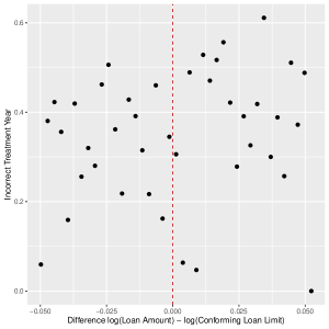
(a) Hurricane Frances (2004)

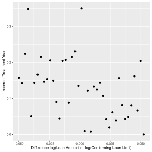
(b) Hurricane Katrina (2005)

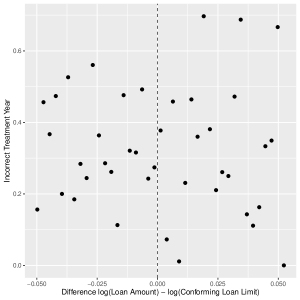
(c) Hurricane Isaac (2012)

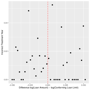
(d) Hurricane Matthew (2016)

Table 2: Errors in LaCour-Little et al. (2022) – A Formal Test of the Peak of Hurricane Treatment Year Errors at the Conforming Loan Limit

This table presents a formal test that the miscoding of treatment years peaks at the conforming loan limit in the data of lacour2022adverse. We perform a regression discontinuity design estimation at the conforming loan limit. The dependent variable is 1 if the year of treatment was miscoded. For instance, as Table 1 shows, observations for many hurricanes in lacour2022adverse are mistakenly coded in a different year. Many Katrina observations are treated in 2004, 2008, and 2012. In this case, the dependent variable is 1. The right-hand side of each regression has the discontinuity and a polynomial of order 1 (column 2), 2 (column 3), 3 (column 4) in the log difference of the loan amount with the conforming loan limit. Standard errors are double-clustered at the ZIP and year level. The number of observations is the number of treated observations at any point between $t-4$ and $t+4$ in lacour2022adverse.

Dependent Variable:	1 if Incorrect Treatment Year
Model:	(1)	(2)	(3)	(4)
Variables
(Intercept)	0.0741∗∗∗	0.0507∗	0.0391	0.0298
	(0.0255)	(0.0277)	(0.0231)	(0.0272)
Below Conforming Limit	0.0541∗∗∗	0.0847∗∗∗	0.0999∗∗∗	0.1121∗∗∗
	(0.0184)	(0.0283)	(0.0268)	(0.0322)
$\Delta\log(\textrm{Loan Amount})$		7.980∗∗	9.818∗∗∗	11.29∗∗∗
		(3.373)	(3.229)	(3.866)
$\Delta\log(\textrm{Loan Amount})^{2}$			4.686∗∗	5.353∗∗
			(1.796)	(1.956)
$\Delta\log(\textrm{Loan Amount})^{3}$				-3.504
				(2.195)
Fit statistics
Observations	173,870	173,870	173,870	173,870
R2	0.00518	0.00710	0.00812	0.00870
Adjusted R2	0.00517	0.00709	0.00810	0.00867
Clustered (ZCTA5 & as_of_year) standard-errors in parentheses
Signif. Codes: ***: 0.01, **: 0.05, *: 0.1

The replication package of these authors was accessed in March 2023 and is stored for your convenience at http://www.ouazad.com/papers/lacour_little_data_archive.zip.

There are other important errors in the paper. A major issue is the incorrect event study design. As the data set has a flat longitudinal structure, this subjects the analysis to the classic issue of the staggered difference-in-differences problem. We display in the table below the sum of the indicator variables for $Time=-4$ to $Time=+4$. In ouazad2022mortgage, this sum is always equal to 1 in the treatment group. Surprisingly, in the lacour2022adverse, this sum can be 0, 2, or 3. This is not due to the reference dummy variable since $\mathbf{1}(Time=0)$ and $\mathbf{1}(Time=-1)$ are included in the sum. Therefore we are observing two major anomalies in the analysis: first, that there are observations with multiple time dummy variables equal to 1 at the same time. 653 mortgages have $\mathbf{1}(Time=+1)$ and $\mathbf{1}(Time=+2)$ equal to 1 at the same time. 568 mortgages have $\mathbf{1}(Time=+2)$ and $\mathbf{1}(Time=+3)$ equal to 1 at the same time. Perhaps even more surprising is that a large chunk of treated observations ($Treatment=1$) may have no dummy at all equal to 1 at any point from $Time=-4$ to $Time=+4$ , i.e. $\sum_{k}\mathbf{1}(Time_{it}=k)=0$. This suggests that the regression’s reference point is incorrectly specified, since the control group will include observations in the pre- and post-treatment periods.

Table 3: Errors in LaCour-Little et al. (2022) – Missing Time Indicator Variables

This table presents, for the treatment group only, the sum of the indicator variables for the number of years relative to the hurricane. In a well-designed event study, each treated observation should have only one time dummy variable equal to 1. Except for the reference time period (e.g. $-1$). In contrast, in LaCour-Little (2022), more than 93,000 observations are in the treatment but have no corresponding time dummy. And more than 6,200 observations have multiple time dummies equal to 1 at the same time. There is no dummy variable for times before $-4$ and no dummy variable for times after $+4$.

	$\sum_{k=-4}^{k=+4}\mathbf{1}(Time_{it}=k)$
	0	1	2	3
Number of Treated Observations	93,231	35,885	6,057	161

Finally, although the sample is extended to 2020, it does not include any billion-dollar hurricane for that time period such as hurricane Harvey (2017). This means that treated observations may be part of the control group.

The evidence presented in this section suggests that lacour2022adverse exhibits major flaws that render the results uninterpretable.

3.2 Rounding of Loan Amounts in Home Mortgage Disclosure Act Data

The previous section has displayed major errors in the empirical work of lacour2022adverse. There are interesting points worthy of further investigation in lacour2022adverse. The first one is that the rounding of loan amounts in HMDA affects the estimation and the fix suggested by lacour2022adverse. The second point is that high cost counties’ conforming loan limits play a significant role in the estimation. We investigate both of these points in turn to see if they affect evidence on the Climate Securitization Hypothesis.

Intuition and Descriptive Statistics

In Home Mortgage Disclosure Act data, loan amounts are reported by rounding loan amounts to the nearest thousand. For instance, on page 12 of the 2013 “Guide to HMDA Reporting, Getting It Right!”:

Loan amount. Report the dollar amount granted or requested in thousands. For example, if the dollar amount was $95,000, enter 95; if it was $1,500,000, enter 1500. Round to the nearest thousand; round $500 up to the next thousand. For example, if the loan was for $152,500, enter 153. But if the loan was for $152,499, enter 152.

Figure 3, case #1, shows what this implies for the difference between actual loan amounts and observed loan amounts when zooming in on, for instance the range of loan amounts between $424,000 and $425,000. This range is relevant for Clay County, Florida, which had a conforming loan limit of $424,100. Loan amounts between 424 and 424.5 (not included) are reported as 424, and loan amounts between 424.5 (included) and 425 are reported as 425. The conforming loan limit is the vertical green dotted line. In this case, only loans between 424 and 424.1 can be conforming loans, but when rounding, all loans between 424 and 424.5 (not included) are reported as conforming. This overestimates the number of conforming loans.

Case #2 suggests that the rounding can also lead to an underestimation of the number of conforming loans. In the case of Collier Count, Florida, the limit is 450.8. Loans between 450 and 450.5 (not included) are counted as conforming, while the true count is larger, as it should include 450 to 450.8. On balance thus, the approach employed in Ouazad and Kahn (2022) leads to symmetric noise. In practice also, the $\pm 10\%$ or $\pm 5\%$ around loan amounts is substantially wider than $1000, ranging from 381 to 467, leading to fewer rounding issues than Figure 3 would suggest.

lacour2022adverse argues that:

“The correct comparison would round the conventional (sic) loan limit in the second term above to the nearest $1000, so that the variable "diff_log_loan_amount" becomes zero and the loan is correctly classified as being at or below the FHA conventional limit.” (page 34 of the October 31, 2022 version, accessed in January 2023, emphasis is ours).

We show below that this approach is incorrect as the share of conforming loans systematically upward biased. In both cases #1 and #2 of Figure 3, the lacour2022adverse approach would count all loans between 424 and 425 (case #1) and between 450 and 451 (case #2). This uses the red dotted line in both graphs. While it generates bunching graphs with no overlapping point (and thus “seem cleaner”) it leads to high and systematic levels of misclassification.

The econometric exercise performed below estimates the properties of the discontinuity estimator implied by Ouazad and Kahn’s (2022) approach with those estimators implied by the lacour2022adverse approach. The exercises suggests that LLPW estimators exhibit larger variances, less precision, higher absolute biases, and slower speeds of convergence to their asymptotic value.

A third approach, not suggested in lacour2022adverse, is to round the conforming loan limit in the same way as for HMDA loan amounts, to the nearest integer. It is easy to see that it also does not address this issue as it leads to greater over- or underestimation of the share of conforming loans. Overall, the approach of ouazad2022mortgage leads to the smallest bias and variance across the three approaches.

3.3 The Rounding of Loan Amounts: Simple Notations and the Economics of Rounding

We can deepen our understanding of the impact of the rounding of loan amounts by (a) understanding under what restrictive set of assumptions the lacour2022adverse approach is correct (always bunching) and (b) by performing an econometric analysis of the estimators using both the lacour2022adverse approach and the ouazad2022mortgage approach. Such econometric analysis will measure the bias and the precision of the estimators.

The true amount of loan $i$ denoted $L_{i}^{*}$ is a latent (unobserved) variable in HMDA, unless one relies on private data sets such as those sold by Corelogic. The observed loan amount $L_{i}$ is the true loan amount $L_{i}^{*}$ rounded to the nearest integer. This can be denoted as $L_{i}=\lfloor L_{i}^{*}\rceil$.

Let’s then denote by $\overline{L}^{*}$ the conforming loan limit in the county of loan $i$. A necessary (but not sufficient) condition for a loan to be conforming is that the true loan amount $L_{i}^{*}\leq\overline{L}^{*}$. We denote this binary variable by $C_{i}^{*}=\mathbf{1}(L_{i}^{*}\leq\overline{L}^{*})$ the classification of loan $i$. One can see that comparing the reported HMDA loan amount $L_{i}$ to the exact conforming loan limit $\overline{L}^{*}$ may lead to an imperfect classification. We denote a HMDA-based classification as$C_{i}^{H}=\mathbf{1}(L_{i}\leq\overline{L}^{*})$. Thus at this stage we have two binary indicator variables: $C_{i}^{*}\in\{0,1\}$ for the true classification (conforming is 1), and $C_{i}^{H}\in\{0,1\}$ for the HMDA-based classification.

Using data where numbers are not rounded is an obvious albeit non-free solution. Using expensive data hinders the public debate over the climate securitization hypothesis.

lacour2022adverse suggests rounding the limit up. This leads to a third classification, denoted $C_{i}^{LL}=\mathbf{1}(L_{i}\leq\lfloor\overline{L}^{*}\rceil)$. It is easy to see that across all classifications $C_{i}^{*}$ (the true one), $C_{i}^{H}$ (the one inferred from HMDA), $C_{i}^{LL}$ (the LaCour-Little), the LaCour-Little approach generates the highest share of conforming loans:

$$C_{i}^{LL}\geq\max\{C_{i}^{*},C_{i}^{H}\}$$ (1)

This is visible on Figure 3. Meanwhile, the HMDA-based classification $C_{i}^{H}$ can either be higher or lower than the true classification $C_{i}^{*}$:

$$\text{There are mortgages $i$ and $j$ such that }C_{i}^{H}\geq C_{i}^{*},\quad\text{and}\quad C_{j}^{*}\geq C_{j}^{H}$$ (2)

This is a first hint that the measure $C_{i}$ will be less biased than the LaCour-Little approach.

The gap between the HMDA-based classification $C_{i}^{H}$ and the LaCour-Little specification $C_{i}^{LL}$ depends on the share of mortgages in the jumbo segment. Perhaps surprisingly, the LaCour-Little approach $C_{i}^{LL}$ is equal to the true classification $C_{i}^{*}$ only when all mortgages are always bunched in the conforming segment, i.e. when there is no jumbo loan in the window. This is unlikely to be true.

The main reason that the is that there are sizeable jumbo applications and originations around the conforming loan limit even for narrow windows. The volume of jumbo mortgage applications and originations does not decline as the window narrows. This is likely due to a few factors. First, the agencies retreated from the mortgage market in 2004-2008, in the wake of the accounting irregularities; this matches the expansion of the private-label mortgage market. Second, a significant share of borrowers choose to borrow using jumbo loans due to either the characteristics of their house or their FICO or LTV.

Table 4: The Share of Jumbo Loans Remains Substantial Even Close to the Conforming Loan Limit

This table presents the share (column 2) of loans with loan amounts above the conforming loan limit, for each size of the window around the conforming loan limit. This suggests that the method suggested by lacour2022adverse, of rounding up the conforming loan limit, would misclassify approximately 27 to 30% of mortgages as conforming when they are jumbo. The window size is the $\max\log(\textrm{Loan Amount})-\log(\textrm{Conforming Limit})$.

(1)	(2)
Window Size	Share of Jumbo Loans $\in[0,1]$
$\pm 1\%$	0.297
$\pm 2\%$	0.289
$\pm 3\%$	0.283
$\pm 4\%$	0.290
$\pm 5\%$	0.277
$\pm 10\%$	0.283
$\pm 15\%$	0.278
$\pm 20\%$	0.278

3.4 Mismeasurement of Bunching in the Cross-Section using LaCour-Little et al.’s (2022) Rounding

lacour2022adverse suggests that conforming loan limits should be rounded up, “The correct comparison would round the conventional (sic) loan limit in the second term above to the nearest $1000.” We examine the econometric properties of such an approach below and suggest that this alternative approached yields biased and imprecise estimators.

Econometric Framework and Monte Carlo Tests in the Cross-Sectional Bunching Case

We conduct Monte-Carlo tests to assess the econometric properties of discontinuity estimators when using either the true measure, the Ouazad and Kahn (2022) approach, and the lacour2022adverse approach. We do so by following standard econometric practice. We postulate a true model and estimate the parameters using either of the imperfect classification methods $C_{i}^{H}$ (Ouazad and Kahn (2022)) or $C_{i}^{LL}$ (lacour2022adverse).

The true model here is one where the probability of approval $P(\text{Approval}_{i}=1)$ is discontinuous at the true conforming loan limit. This is modelled as a logit:

$$P(\text{Approval}_{i}=1)=P(\text{Approval}_{i}^{*}\geq 0)=P(\alpha^{*}+\beta^{*}C_{i}^{*}-\varepsilon\geq 0)$$ (3)

The true model depends on the true classification $C_{i}^{*}$. Of course, in econometric practice, the probability of approval depends on a host of covariates such as the creditworthiness of the borrower, the location and characteristics of the house, the characteristics of the lender. The insights of our approach extend to this more general class of econometric models.

Bunching at the conforming loan limit can be estimated in multiple ways. A popular approach is to consider an OLS regression. Another approach, which we leave to the reader for further analysis, is a logit regression. As logit regressions entail other issues such as incidental parameter problems [chamberlain1980analysis, lancaster2000incidental] when including fixed effects in a more comprehensive regression. We thus focus on the least squares approach.

The data is generated according to 3. The regression is:

$$\text{Approval}_{i}=\hat{\alpha}^{s}+\hat{\beta}^{s}C_{i}^{s}+\epsilon_{i}^{s},$$

where $s\in\{*,H,LL\}$ is the choice of the classification of the loan: using the true discontinuity, using the HMDA discontinuity, and using the conforming loan limit. $\hat{\beta}^{*}$ is the OLS estimate based on the true discontinuity. We compare $\hat{\beta}^{H}$ and $\hat{\beta}^{LL}$ to $\hat{\beta}^{*}$.

Results for the Static Bunching Case

We consider a case with $N=1,000$ observations, true values $\alpha=0.2$ and $\beta=0.1$, and $S=10,000$ simulations. Each approval decision is 1 with probability $F(\alpha^{*}+\beta^{*}C_{i}^{*})$, where $F$ is the cdf of the logit.

The first visible statistic is that across the two methods, the LaCour-Little approach is that which misclassifies loans more extensively. In the Monte Carlo samples, misclassifications are as follows:

County	Share Misclassified HMDA	Share Misclassified LLPW
Clay County, Florida	0.006	0.014
Collier County, Florida	0.010	0.010

This table suggests that in the case of Clay County the share of misclassified loans (1.4%) with the lacour2022adverse approach is more than double (0.6%) that of the HMDA approach of ouazad2022mortgage. In the case of Collier county, the share misclassified is the same in both the HMDA approach and the LLPW overestimate the share of conforming loans. Overall, using HMDA loan amounts provides a lower share of misclassifications.

We then turn to the regression results. Figure 3 presents the distribution of the difference between the estimator $\hat{\beta}^{H}$ obtained using the HDMA loan amounts as in ouazad2022mortgage and the estimator $\hat{\beta}^{*}$ on true data with no misclassification. This is the blue line. The distribution of the difference $\hat{\beta}^{LL}-\hat{\beta}^{*}$ is the orange line. As the graph makes clear in both case 1 (subfigure (a), Clay County, FL) and in case 2 (subfigure (c), Collier County, FL), the lacour2022adverse is exhibits higher standard deviation, while ouazad2022mortgage approach yields only a minor increase in standard deviation compared to the estimator using the true classification. Subfigures (b) and (d) present the distribution of the absolute difference $|\hat{\beta}^{s}-\hat{\beta}^{*}|$ for $s=H$ and for $s=LL$. In both cases, the absolute bias is higher in the lacour2022adverse than with ouazad2022mortgage approach.

Figure 4 shows that the estimator based on lacour2022adverse performs worse regardless of sample size. Subfigure (a) displays the absolute deviation $|\hat{\beta}^{s}-\hat{\beta}^{*}|$ from the true value for sample sizes ranging from 50 to 2000. The absolute deviation is substantially higher at all $N$s. Subfigure (b) shows that the estimator is also less precise. The standard deviation of lacour2022adverse estimator is higher at all $N$s.

Conclusion

HMDA loan amounts are rounded to the nearest integer. Conforming loan limits are typically at an exact multiple of thousands of dollars. With HMDA, the approach of ouazad2022mortgage yields the smallest share of misclassifications, a lower absolute deviation, and is more precise. While using private data with exact loan amounts (e.g. Corelogic data) would address this issue, this is not what lacour2022adverse suggest, and their approach yields biased and imprecise estimators.

3.5 Point #2: The Role of High Cost Counties’ Specific Conforming Loan Limits

The Geographic Distribution of High-Cost Counties

Conforming loan limits vary by county and by year, as noted by ouazad2022mortgage. In any given year, roughly 100 to 200 counties (out of 3,143) are deemed “high-cost counties.” Figure 6 presents a map of conforming loan limit $ by county, and delineates the boundaries of states of the Atlantic coast and the Gulf of Mexico. These are the states most exposed to hurricanes and are thus the focus of any analysis of the impact of hurricanes on mortgage securitization. Figure 6 suggests that most coastal counties are not high cost counties. Many high cost counties are in the San Francisco Bay Area, the Los Angeles area, and the Seattle area. A notable exception is the New York City area, which both experienced Hurricane Sandy in 2012 and is a high-cost area. Yet, there is no difference between ouazad2022mortgage and lacour2022adverse conforming loan limits in the New York metropolitan area. This is a first intuitive indication that the quantitative importance of lacour2022adverse point may be small. The next section investigates this point.

4 Testing the Climate Securitization Hypothesis:
Securitization Dynamics in the Aftermath of Natural Disasters

We reestimate ouazad2022mortgage baseline specification using the limits provided by lacour2022adverse. The results are presented on Figure 7 for all three outcome variables, approval, origination, and securitization conditional on approval. They are similar to the original findings in ouazad2022mortgage Figure 8. Tables 5 to 7 provide further statistical tests for each bandwidth. The null hypothesis here is that the lending standards in the conforming segment are not differentially changing after a billion-dollar disaster relative to the overall market. A rejection of the null hypothesis with a positive and statistically significant estimate for approval or origination rates suggests that lending standards are becoming more lenient in the conforming segment as compared to the jumbo segment. This is what Figure 7 suggests: approval probabilities increase gradually all the way to $+6$ percentage points in year 3 (subfigure (a)), the origination probabilities increase all the way to $+5$ percentage points in year 3 (subfigure (c)), and the probability of securitization conditional on origination increases by approximately 12 percentage points in year 4 (subfigure (e)). The bars indicate the double-clustered standard errors at the ZIP and year levels.

The timing is also similar to ouazad2022mortgage: in the first 3 years following a natural disaster, approval, origination rates increase significantly and then taper off. In the third and fourth year, securitization rates $P(\text{Securitized}|\text{Originated})$ increase in turn, suggesting that lenders are changing their securitization practices in the conforming segment conditional on origination. For each figure, the right-hand column is for the impact on the mortgage market regardless of the conforming segment. There there is a systematic decline in approval, origination, and securitization rates: approval rates decline by up to 7 percentage points (subfigure (b)), origination rates by 7 percentage points as well (subfigure (d)), and securitization rates by up to 10 percentage points (subfigure (f)), indicating that the origination and securitization activity in the jumbo segment tapers off significantly after a natural disaster. This is likely due to both the difficulty of securitizing jumbo loans in the private label market and the reluctance of lenders to originate and hold.

Hence what likely explains the difference between lacour2022adverse and ouazad2022mortgage is the significant errors of lacour2022adverse documented in Section 3.1 and the incorrect rounding of conforming loan limits.

Inspecting the Mechanism: Treatment Effects at Each Distance of the Conforming Loan Limit

What drives the results of both ouazad2022mortgage and this paper? Is the effect driven by treatment effects far away from the conforming loan limit, or by sharp discontinuities exactly at the limit? The approach described in this section provides appealing and intuitive graphical approaches to an understanding of the main treatment effects, presented Figures 8–10. Open source code is available at the link on the cover page.

To understand the method, consider a distance $\delta\in[-0.10,+0.10]$ to the conforming loan limit. We would like to estimate the impact $\text{TE}(\delta)$ of a billion dollar event on approval probabilities exactly at $\delta$. We also would like to control for year, ZIP, and disaster confounders, as in the main regression. This is performed by estimating the coefficients $\xi_{t}$ for $t=-4,-3,-2,0,1,2,3,4$ that minimize:

$$\min \sum_{it}\left(\text{Approval}_{it}-\sum_{t=-4}^{+4}\xi_{t}(\delta)\cdot\text{Treated}_{j(i)}\times\textrm{Time}_{t=y-y_{0}(d)}\right.$$

$$\qquad\qquad\qquad\qquad-\textrm{Year}_{y(t,d)}-\text{Disaster}_{d}-\text{ZIP}_{j(i)}\Biggr{)}^{2}K\left(\frac{\Delta\text{Loan Amount}_{it}-\delta}{h}\right)$$ (4)

while weighting observations by their distance $\Delta\text{Loan Amount}_{it}-\delta$. Hence when $\delta=-0.10$, the coefficients $\xi_{t}(\delta)$ measure the treatment effect for loan amounts 10% below the conforming loan limit. When $\delta=+0.10$, the coefficients $\xi_{t}(\delta)$ measure the treatment effect for loan amounts 10% above the conforming loan limit. $K$ is a Gaussian kernel and we use the bandwidth $h=1\%$. Robustness to bandwidth choice is presented on Tables 5–7. When considering $\delta<0$, the treatment effects are estimated using observations in the conforming segment. When $\delta>0$ the treatment effects are estimated using observations in the jumbo segment.

An advantage of this approach is it flexibility and its visual representation. A drawback may be the difficulty of obtaining standard errors; this is addressed in the next subsection where discontinuities at the conforming loan limit are formally tested using double clustering at the Year and ZIP levels.

Figure 9 presents the estimation results for the approval rate, using 40 distances, and a bandwidth of 1%. Subfigure (a) is for the treatment effects at time $t=+1$, (b) for time $t=+2$, (c) for time $t=+3$, (d) for time $t=+4$. The graph suggest that most of the treatment effects occur at the conforming loan limit. In time $t=+1$, the approval rate declines for jumbo loans in the two bins at the immediate right of the limit, while the treatment effects in the jumbo segment for loan amounts from 2.5 to 10% above the limit are similar to treatment effects in the conforming segment. In time $t=+2$, the situation changes drastically: the treatment effects drop sharply for almost all loan amounts in the jumbo segment, and the discontinuity (drop) in approval rates is visible at the conforming loan limit. A similar scenario appears in time $t=+3$ (subfigure (c)). In time $t=+4$, we should not expect a discontinuity in approval rates, as documented earlier and consistent with the baseline findings of both this paper (Figure 7) and ouazad2022mortgage Figure 8.

Figure 8 presents the estimation results when the outcome variable is the origination rate of mortgage applications. Mortgages are originated when they are approved by the lender and accepted by the borrower. The picture is qualitatively similar to those for the approval rate (Figure 9), suggesting that it is not borrowers’ behavior that is driving results, but rather lenders.

Figure 8 presents the estimation results when the outcome variable is the securitization rate of mortgage originations. We should expect these results to be different from those of the origination and approval rates, given that the securitization probabilities conditional on origination picks up in years +3 and +4. In practice, we observe that there are discontinuities in the impact of billion dollar disasters on securitization probabilities in each time period $t=+1$ to $t=+4$. The discontinuity in the treatment effect become large: over +10 percentage points in time $t=+3$, over +16 percentage points in time $t=+4$. The next subsection provides a formal significance test of these discontinuities controlling for the year, ZIP, disaster confounders, and the interaction of year, ZIP, disaster f.e.s with the discontinuity as in ouazad2022mortgage.

Regression Discontinuity Bandwidth and Estimation Results

The previous section 4 suggested that a significant part of the mechanism underlying the securitization hypothesis is at the limit or in a window around the limit. This suggests the use of the regression discontinuity framework, for which an extensive literature provides methodological guidance, including imbens2008regression and cattaneo2022regression. The approach here performs such regression discontinuity while keeping the same of controls and fixed effects that are present in the baseline specification ouazad2022mortgage: year, ZIP, disaster, year$\times$Below the conforming loan limit.

The regression discontinuity estimator of the impact of a billion dollar event is estimated as in cattaneo2022regression. We set $\delta=0$ (at the limit) in specification 4 and start by estimating the treatment effects exactly on the left side of the conforming loan limit:

$$\min \sum_{it}\left(\text{Approval}_{it}-\sum_{t=-4}^{+4}\xi_{t}(\delta)\cdot\text{Treated}_{j(i)}\times\textrm{Time}_{t=y-y_{0}(d)}\right.$$

$$\qquad\qquad\qquad\qquad-\textrm{Year}_{y(t,d)}-\text{Disaster}_{d}-\text{ZIP}_{j(i)}\Biggr{)}^{2}K\left(\frac{\Delta\text{Loan Amount}_{it}}{h}\right),$$ (5)

for $\Delta\text{Loan Amount}_{it}<0$ (conforming segment). This yields estimates of treatment effects $\xi_{t}(\delta=0^{-})$. We do the same estimation, but setting $\delta=0$ and considering only mortgages of the jumbo segment. This yields estimates of treatment effects $\xi_{t}(\delta=0^{+})$. As in cattaneo2022regression, the impact of a billion-dollar disaster on the discontinuity in approval rates at the conforming loan limit is:

$$\tau_{RD}=\xi_{t}(\delta=0^{-})-\xi_{t}(\delta=0^{+})$$ (6)

The innovation here is that we estimate the impact of billion dollar disasters on the regression discontinuity controlling for the Year fixed effects, the Disaster specific fixed effects, the ZIP code fixed effects. Since the fixed effects are different on each side of the conforming loan limit, this also controls for year $\times$ below limit, $ZIP$ $\times$below limit and disaster $\times$ below limit confounders.

This RD design of cattaneo2022regression is straightforward to implement. It corresponds to the regression:

$$Outcome_{it} =\alpha\cdot\text{Below\,Conforming\,Limit}_{ijy(t,d)}+\gamma\text{Below\,Conforming\,Limit}_{ijy(t,d)}\times\text{Treated}_{j(i)}$$

$$\quad\quad+\sum_{t=-T}^{+T}\xi_{t}\cdot\text{Treated}_{j(i)}\times\text{Time}{}_{t=y-y_{0}(d)}$$

$$\quad\quad+\sum_{t=-T}^{+T}\tau_{t}\cdot\text{Below\,Conforming\,Limit}_{ijy(t,d)}\times\text{Treated}_{j(i)}\times\text{Time}{}_{t}$$

$$\quad\quad+\sum_{y=1995}^{2016}\zeta_{y}\cdot\text{Below\,Conforming\,Limit}_{ijy(t,d)}\times\text{Year}{}_{y(t)}$$

$$\quad\quad+\sum_{d}\chi_{d}\cdot\text{Below\,Conforming\,Limit}_{ijy(t,d)}\times\text{Disaster}_{d}$$

$$\quad\quad+\sum_{j}z_{j}\cdot\text{Below\,Conforming\,Limit}_{ijy(t,d)}\times\text{ZIP}_{j(i)}$$

$$\quad\quad+\text{Year}{}_{y(t,d)}+\text{Disaster}{}_{d}+\text{ZIP}{}_{j(i)}+\varepsilon_{it},$$ (7)

weighted by the distance of each loan to the conforming loan limit $K\Biggl{(}\frac{\Delta\textrm{Loan Amount}_{it}}{h}\Biggr{)}$. The parameters of interest are the treatment effects $\tau_{t}$ for $t=1,2,3,4$. They measure the discontinuity in treatment effects at the conforming loan limit.

We use a Gaussian kernel for $K(\cdot)$, popular in a number of seminal papers such as dinardo1996labor, connor2012efficient, duclos2004polarization, barone2008garch. This fixed effect panel regression is similar to the main specification of ouazad2022mortgage, where observations are weighted by the values $K_{i}=K\left(\frac{\log L_{i}-\log\overline{L}^{*}}{h}\right)$ and the bandwidth $h$ varies between 1% and 20%. The standard errors are double-clustered by ZIP and year.

Tables 5–7 present the results. For each table, the upper panel is for bandwidths $h$ of 1% to 4%, in increments of 1 ppt. The lower panel is for bandwidths $h$ of 5, 10, 15, 20%. Table 5 is for the approval rate, Table 6 is for the origination rate, Table 7 for the securitization rate in the universe of originated mortgages.

Each table reports both the impacts for the mortgage market ($\text{Treated}_{j(i)}\times\text{Time}{}_{t=y-y_{0}(d)}$ indicator variables) and for the conforming market ($\text{Below\,Conforming\,Limit}_{ijy(t,d)}\times\text{Treated}_{j(i)}\times\text{Time}{}_{t}$ indicator variables).

Results suggest that the bandwidth of 1% to 3% maximizes the mean squared error for the approval and origination outcome variables respectively. Results suggest that billion dollar disasters increase the discontinuity in approval probabilities by up to 6.48% (**), increase the discontinuity in origination probabilities by 6.08% (**), and the discontinuity in securitization probabilities by up to 17.7% (***). The timing of the effects also matches the timings of the main regression: an increase in approval and origination rates, followed by an increase in securitization rates. The code is available at https://www.ouazad.com/paper/code_2023_05.zip.

5 Policy Trade-Offs: Market Pricing of Climate Risk and Bluelining

5.1 Flexible Market-Based Guarantee Fees

When lenders securitize their mortgages by selling them to the Government Sponsored Enterprises Fannie Mae and Freddie Mac, they transfer the risk of delinquency and default in exchange for the payment of a guarantee fee. These guarantee fees are presented in a Loan Level Performance Adjustment matrix, as a number of basis points of the balance of the loan. Guarantee fee reports of the Federal Housing Finance Agency (FHFA) suggest that g-fees are independent of climate risk.

Under the Climate Securitization Hypothesis, lenders may take advantage of securitization whenever either their estimates of losses for a specific mortgage are higher than g-fees, when lenders are risk averse – and thus their risk neutral probability of losses is higher than the g-fees –, or when private label securitization offers a greater income than government securitization. This may happen as (1) g-fees do not depend on climate risk including forecasts of drought, wildfires, hurricane storm surges, riverine flooding and (2) lenders may develop expertise, human capital, and data science to assess climate risk at a granular level.

Guarantee fees are not set by a competitive process of auctions or the meeting of bid and ask on a market as in duffie2005over. Rather, guarantee fees are set by the Federal Housing Finance Agency as the outcome of an administrative and political process. deritis2014general outlines three rules for setting g-fees at an appropriate level: (1) ensuring an appropriate level of capital, and layton2023 suggests that the average g-fee has been between 0.45 and 0.49% since 2014, lower than the level that allow Fannie Mae and Freddie Mac to reach its capital standard. (2) g-fees with acceptable redistributive properties, such as lower g-fees for lower income households; this paper suggests that g-fees may be adjusted to be a function of both climate risk and other parameters such as FICO, LTV, DTI. The pass-through of such g-fees into mortgage interest rates would incentivize adaptation efforts [kahn2021adapting] in the form of greater screening  and greater self-protection [ehrlich1972market]. (3) g-fees should be set taking into account the elasticity of the supply of loans to the agencies; yet, recent increases in the market share of GSE loans combined with the decline in both unsecuritized first liens and private-label MBSs suggest that the supply of loans has low elasticity w.r.t. to the g-fees at their current level.

Figure 2: Loan Level Price Adjustment matrix on May 5th, 2023

This table presents the guarantee fees (g-fees) charged by Fannie Mae for the securitization of purchase money loans. Additional g-fees may be charged for condos, ARMs, investment properties, second homes, high balance loans, and high DTI ratios above 40%.

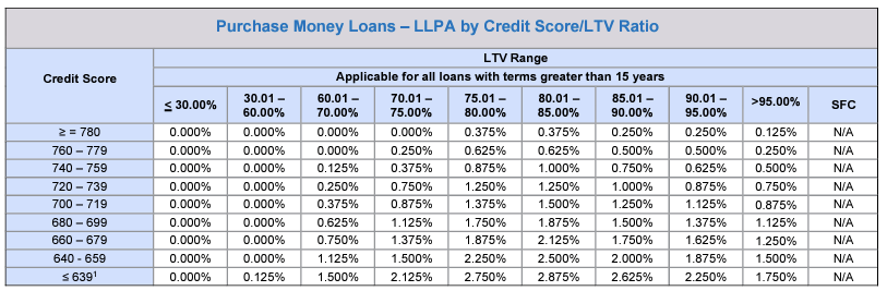
Source: https://singlefamily.fanniemae.com/media/9391/display .

Aside from guarantee fees, the impact of climate risk on the agencies may be mitigated by (1) flood insurance policies, (2) private mortgage insurance, (3) credit risk transfers such as Connecticut Avenue Securities. We examine these in turn.

The 10-K filing of Fannie Mae for the fiscal year ended December 31, 2022 suggests that flood insurance policies covering homes under the National Flood Insurance Program may have a limited impact on credit losses.

Only a small portion of loans in our guaranty book of business as of December 31, 2022 was located in a Special Flood Hazard Area, for which we require flood insurance: 3.3% of loans in our single-family guaranty book of business and 6.8% of loans in our multifamily guaranty book of business. We believe that only a small portion of borrowers in most places outside of a Special Flood Hazard Area obtain flood insurance. The risk of significant flooding in places outside of a Special Flood Hazard Area (that is, in places where we do not require flood insurance) is expected to increase in the coming years as a result of climate change.

cohen2021storm suggests that natural disasters such as hurricane Sandy provide new news about the location of flood risk beyond the boundaries of the Special Flood Hazard Areas.

Private Mortgage Insurance covers mortgages with loan-to-value (LTV) ratios above 80%. The minimum balance covered for fixed-rate mortgages with a 30-year maturity is 6% for mortgages with an LTV between 80 and 85%, 12% for mortgages between 85 and 90%, and between 16 and 35% for mortgages with LTVs above 90%. deritis2014general suggests that on average PMI covers 27.5% of the balance. bhutta2022moral studies the PMI market and suggests that there is little variation in premia across places or across private mortgage insurers, and thus competition in this market is primarily in volume rather than pricing. Hence PMI pricing incentives are not correlated with climate risk. Finally, 2022 10-K filings suggest that “Although our primary mortgage insurer counterparties currently approved to write new business must meet risk-based asset requirements, there is still a risk that these counterparties may fail to fulfill their obligations to pay our claims under insurance policies.” Hence the impact of climate risk on the agencies’ net income and capital depends on the magnitude of the impact of climate risk on delinquencies and defaults.

The third and most recent approach to hedging credit losses is the Credit Risk Transfer program. gete2022climate collect CRT yield data and study the response of such yields to differential exposure to hurricanes Irma and Harvey. These CRT yields have the potential of providing market-implied g-fees, and the authors suggest that they would be 10% higher than the current g-fees in counties most exposed to hurricanes and 35% lower in inland counties. Translated into the current LLPA matrix of Figure 2, this suggests that this would be between a 3.75 and 28.75 basis point increase in counties exposed to hurricanes; and a decline between 13 basis points and 100 basis points in inland counties. This paper thus suggests the possibility of adding a third dimension to the LLPA matrix, which would provide both redistribution away from coastal areas and incentives for households to locate in safer areas.

5.2 A Challenging Trade-Off Between Redlining and the Price Signal of Higher Flood Risk

While the efficiency of the mortgage and securitization markets would suggest flexible market-based g-fees, one concern is that such pricing would entail a new form of redlining, the bluelining of hurricane-exposed areas. aaronson2021effects finds substantial welfare consequences of redlining beyond interest rates and the approval rates of mortgage applications: lower homeownership rates, house values, and higher segregation. Thus a key question raised by bluelining is the trade-off between the signal of increased flood risk, which incentivizes moving out of harm’s way vs. the lasting impacts on affordability and homeownership. Such policy trade-off is at the frontier of policy and research discussions.

A key empirical question is whether those areas most at risk of flooding are also areas with lower income households and minority households. Figure 11 presents the descriptive (correlational) relationship between Census demographics and First Street Foundation’s flood risk factor at the Zip level. In these figures we consider four simple metrics: the share white, the median household income, the share on cash public assistance or food stamps/SNAP, and the rent as share of household income. These descriptive plots are not causal, and they also do not control for state or MSA fixed effects, thus the sorting within states and within metropolitan areas may differ from the US-wide sorting depicted in the chart.

The Figure portrays a nuanced set of facts. First, areas at risk of flooding according to First Street have lower median household income. Second, these areas tend to have higher shares of whites. Third, these households spend more on rent as a fraction of household income, and they are also more likely to be on cash public assistance, food stamps or SNAP. This suggests that a geographic pricing of g-fees may have distributional consequences that differ markedly from the historical legacy of FHA or HOLC redlining: households at risk of flooding are more likely to be lower income white households.

6 Conclusion: Adaptation to Climate Risk and the Securitization Market

The Climate Securitization Hypothesis posits that natural disasters increase the probability that lenders originate loans sold to government sponsored securitizers. An emerging natural disaster literature explores how shocks affects many aspects of the real economy [boustan2020effect]. In the real economy, margins of adjustment include migration [deryugina2018economic, smith2022adjusting], home price declines [ortega2018rising, cohen2021storm], and public finance dynamics [healy2009myopic, jerch2023local]. In the financial sector, as investment and consumption are typically leveraged [geanakoplos2010leverage] , margins of adjustment in response to climate risk exposure include the LTV ratios [sastry2021bears, bakkensen2023leveraging], interest rates and yields [goldsmith2022sea, nguyen2022climate], approval rates, amortization structures of loans. In the financial sector, risk is hedged using risk transfers [gete2022climate] and derivative products [ouazad2022investors]. In financial markets, natural disasters may also affect market microstructure and liquidity [rehse2019effects].

A consistent finding in this empirical literature is that natural disasters induce shifts in investment, consumption, and leverage as both households and investors reoptimize in the aftermath of these events. Such natural disasters increase uncertainty [baker2020using]. Natural disasters may also introduce ambiguity about the distribution of future probability distributions, making assets exposed to such ambiguous risks less valuable.

In the aftermath of a natural disaster, physical assets in the affected area can become less valuable and cash flows may decline. In the mortgage market, evidence suggests a higher probability of loan delinquency and default risk in the aftermath of such shocks [ratcliffe2020bad, issler2021housing, holtermans2022climate, biswas2023california, ho2023we, ouazaddiscussion]. Hikes in insurance premia and losses of earning opportunities [indaco2021hurricanes] may cause cash flow shocks that are one of the triggers (one of the double hurdles) of mortgage delinquencies [ganong2023borrowers]. The increased probability of delinquency and foreclosure may be higher if the spatial correlation of the shock is such that many neighboring home owners are simultaneously considering defaulting on their loans, causing foreclosure externalities [gerardi2015foreclosure].

Under the current rules, bank and non-bank lenders in exposed areas have increased incentives to “originate and distribute” loans. This is the Climate Securitization Hypothesis. The securitization option is particularly valuable when losses are either correlated in the lender’s portfolio or if such losses are correlated with the lender’s net income. During a time of more intense natural disasters, this issue takes on a greater importance. If lenders are aware that they can securitize such loans, this weakens their screening incentives and households’ incentive to invest in self-protection.

lacour2022adverse acknowledge this microeconomic logic but claim that the empirical approach does not provide evidence supporting the CSH. In this paper, we have examined their claims and have focused on both the statistical validity and the economic content of their statistical criticisms. In our re-examinination of the evidence, we have made three main points: first, the construction errors of the event study in lacour2022adverse are very serious and render their results uninterpretable. Hurricane years are miscoded. Recent literature provides guidance on the appropriate construction of difference-in-difference event studies [callaway2021difference]. Second, lenders have incentives to originate conforming and jumbo loans even at small distances of the loan amounts to the conforming loan limit, suggesting that not all mortgages in the vicinity of the limit should be classified as conforming. Third, careful and granular analysis of the discontinuities in approval, origination and securitization probabilities suggests that lenders are significantly more likely to originate conforming loans than jumbo loans in the aftermath of a natural disaster. This identification strategy by regression discontinuity design (RDD) at the conforming loan limit identifies the option value of securitization, i.e. the impact of the securitization option on the net income of mortgage originations for lenders.

Our re-examination of the evidence provides confidence in the recent sample evidence supporting the CSH. As future disasters take place, we conjecture that nimble financial markets will play a key role in the climate change adaptation process. Financial engineering helps in the diversification of risk and in designing new assets that complete markets.

First, financial markets will improve the design of pools that either diversify climate risk or provide selected exposure to climate risk factors. Climate risk will change the design of Agency and Private Label Mortgage-Backed Securities. They may also affect the design of To Be Announced (TBA) markets [vickery2013tba] for agency Mortgage-Backed Securities as those currently do not feature climate risk among the observable set of characteristics of traded pools.

Second, financial markets can complete the market with securities that provide cash flows contingent on the realization of risk. This includes catastrophe bonds, insurance linked securities, and weather derivatives.

Figure 3: Rounding and Loan Amounts: Why LaCour-Little et al.’s (2022) Approach Systematically Biases the Counts of Conforming Loans in Two Cases

These figures are an illustration of the rounding of loan amounts to the nearest integer. The true loan amount $L^{*}$ is on the horizontal axis. $L$, the observed loan amount is on the vertical axis. $\overline{L}^{*}$ the true conforming loan limit, is the green line. The conforming loan limit rounded up as in lacour2022adverse is the red line. The lacour2022adverse approach yields a systematic overestimation of the number of conforming loans. In contrast, the approach of ouazad2022mortgage yields either an overestimation (case 1) or an underestimation (case 2) of the number of conforming loans.

(a) Case #1: Clay County, Florida, Limit $424,100

(b) Case #2: Collier County, Florida, Limit $450,800

Figure 4: Bias and Imprecision of the LaCour-Little et al. (2022) rounding approach with Cross-Sectional Bunching Estimators – Bias and Standard Deviation vs Number of Observations

The top panel present the evolution of the absolute deviation $|\hat{\beta}^{s}-\hat{\beta}^{*}|$ with respect to the number of observations in the window around the conforming loan limit, in the Monte Carlo Simulation. The orange line is using the lacour2022adverse approach. The blue line uses ouazad2022mortgage approach. The bottom panel presents the standard deviation $SD(\hat{\beta}^{s})$ of the estimators. Same color code. lacour2022adverse yields higher absolute deviations and higher variances for all sample sizes.

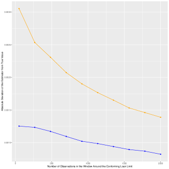
(a) Absolute Deviation of the Cross-Sectional Bunching Estimators from the True Value

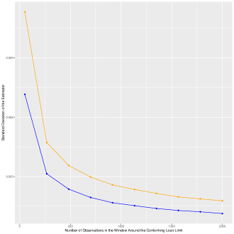
(b) Standard Deviation of the Cross-Sectional Bunching Estimators

The parameters of the Monte Carlo simulations are $N\in[50,2000]$, $\alpha=0.2$, $\beta=0.1$.

Figure 5: Rounding and Loan Amounts: A Monte-Carlo Analysis of Variance and Bias

These figures present the distribution of the difference between the cross-sectional bunching estimator $\hat{\beta}^{s}$ with misclassification and the estimator $\hat{\beta}^{*}$ on the true data. We consider two possible misclassifications: $s=H$ when using the classification of conforming loans using the observed HMDA loan amount and the actual conforming loan limit, as in ouazad2022mortgage; $s=LL$ when the using the LaCour-Little classification based on rounding the conforming loan limit to the highest integer. The LaCour-Little approach leads to higher variance and higher absolute bias.

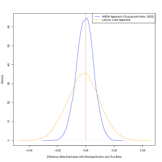
(a) Case #1, Clay County, FL, Distribution of $\hat{\beta}^{s}-\hat{\beta}^{*}$

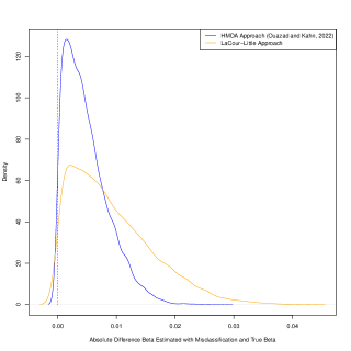
(b) Case #1, Clay County, FL, Distribution of $|\hat{\beta}^{s}-\hat{\beta}^{*}|$

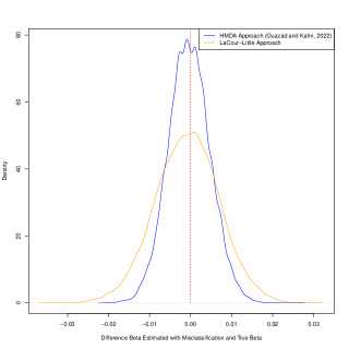
(c) Case #2, Collier County, FL, Distribution of $\hat{\beta}^{s}-\hat{\beta}^{*}$

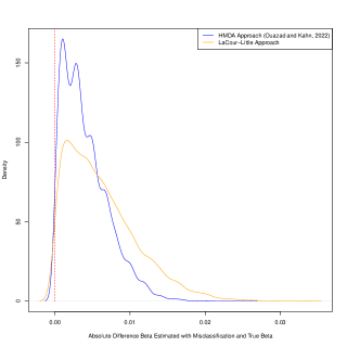
(d) Case #2, Collier County, FL, Distribution of $|\hat{\beta}^{s}-\hat{\beta}^{*}|$

The parameters of the Monte Carlo simulations are $N=1,000$, $\alpha=0.2$, $\beta=0.1$.

Figure 6: Geographic Distribution of Conforming Loan Limits and High Cost Counties

This map presents the county-level conforming loan limit in 2016 (insights are similar when mapping other years post HERA). The white dotted line are the boundaries of the Atlantic states and states of the Gulf of Mexico, where most hurricanes occur and is the focus of ouazad2022mortgage. Most high-cost counties are outside the area of the Atlantic states and the Gulf of Mexico, with the exception of the New York-Newark-Jersey City, NY-NJ-PA metro area. Yet there both lacour2022adverse and ouazad2022mortgage find significant impacts of hurricane exposure on origination probabilities in the conforming segment.

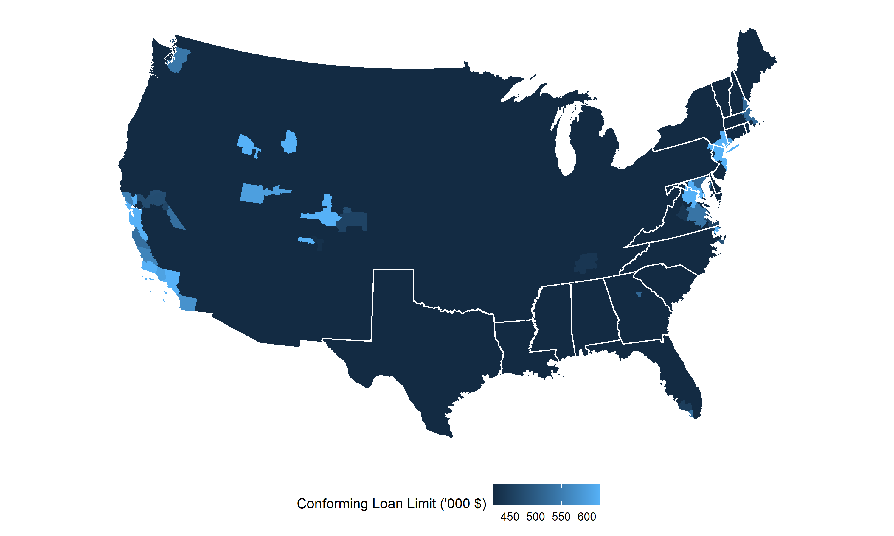
Sources: County shapefile (2014) from the US Census Bureau, conforming loan limits as in lacour2022adverse.

Figure 7: Treatment Effects – Replication of Ouazad and Kahn (2022) with Limits Provided by LaCour-Little (2022)

These four graphics present the impact of a billion-dollar event on the approval, origination rates and securitization conditional on origination for mortgage applications (Section 4). The left column present the impact on conforming loans only (the coefficients of the Below Limit $\times$ Treated $\times$ Time $k$). The right column presents the impact for the entire mortgage market in the window around the conforming loan limit. Confidence intervals at 95% obtained by double-clustering standard errors at ZIP and year levels. These results are similar to ouazad2022mortgage Figure 8 and the source code is available at this link.

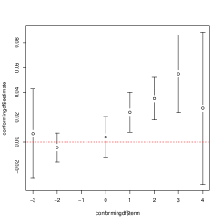
(a) Approval Probabilities, Conforming Market

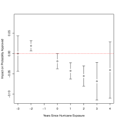
(b) Approval Probabilities, Overall Market

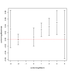
(c) Origination Probabilities, Conforming Market

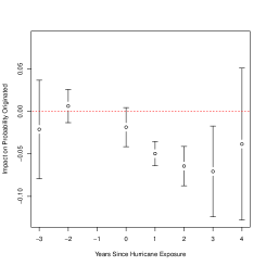
(d) Origination Probabilities, Overall Market

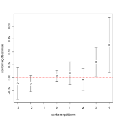
(e) P(Securitization$|$Origination), Conforming Market

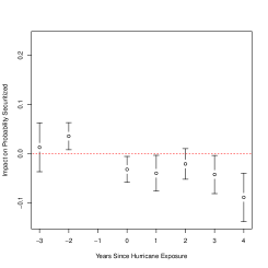
(f) P(Securitization$|$Origination), Overall Market

Open source code available at this link.

Figure 8: Inspecting the Mechanism: Treatment Effect by Distance to the Conforming Loan Limit

The graphs below inspect the mechanism driving the results presented in Figure 7 using local polynomial regressions. Each point in Subfigure (a), (b), (c), (d) is a separate estimation of the impact of a billion dollar disaster on origination rates. For each point, we weigh observations according to the distance to the conforming loan limit.

$$\text{Originated}_{it}=\sum_{t=-4}^{+4}\xi_{t}\cdot\text{Treated}_{j(i)}\times\textrm{Time}_{t=y-y_{0}(d)}+\textrm{Year}_{y(t,d)}+\text{Disaster}_{d}+\text{ZIP}_{j(i)}+\varepsilon_{it}$$

The weights are the kernel $K((\Delta\log\text{Loan\,Amount}-\text{Distance\,to\,Conforming\,Loan\,Limit})/h)$, where each of the 40 regressions uses a different Distance to the Conforming Loan Limit $\in[-0.10,0.10]$. These regressions display flexible results free of assumptions on rounding or on the choice of the window. Figures suggest that (a) the discontinuity at the limit is key to the results, (b) the discontinuity is sharp in time $t=1,2,3$, and smoother in $t=4$. Tests of statistical significance are performed on Table 6.

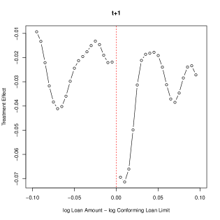
(a) Originated, time $t+1$

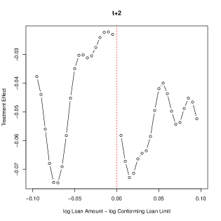
(b) Originated, time $t+2$

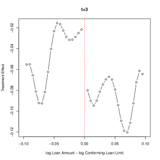
(c) Originated, time $t+3$

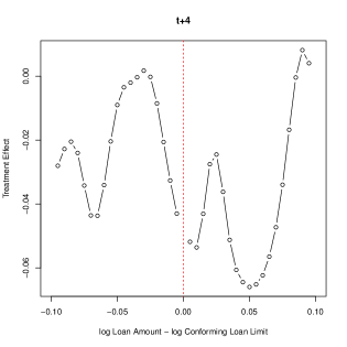
(d) Originated, time $t+4$

Open source code available at this link.

Figure 9: Inspecting the Mechanism: Treatment Effect by Distance to the Conforming Loan Limit

The graphs below inspect the mechanism driving the results presented in Figure 7 using local polynomial regressions. Each point in Subfigure (a), (b), (c), (d) is a separate estimation of the impact of a billion dollar disaster on approval rates. For each point, we weigh observations according to the distance to the conforming loan limit.

$$\text{Approval}_{it}=\sum_{t=-4}^{+4}\xi_{t}\cdot\text{Treated}_{j(i)}\times\textrm{Time}_{t=y-y_{0}(d)}+\textrm{Year}_{y(t,d)}+\text{Disaster}_{d}+\text{ZIP}_{j(i)}+\varepsilon_{it}$$

The weights are the kernel $K((\Delta\log\text{Loan\,Amount}-\text{Distance\,to\,Conforming\,Loan\,Limit})/h)$, where each of the 40 regressions uses a different Distance to the Conforming Loan Limit $\in[-0.10,0.10]$ and the bandwidth $h=1\%$. These regressions display flexible results free of assumptions on rounding or on the choice of the window. Figures suggest that (a) the discontinuity at the limit is key to the results, (b) the discontinuity is sharp in time $t=1,2,3$, and smoother in $t=4$. Tests of statistical significance are performed on Table 5.

(a) Approved, time $t+1$

(b) Approved, time $t+2$

(c) Approved, time $t+3$

(d) Approved, time $t+4$

Open source code available at this link.

Figure 10: What Drives Results? Inspecting the Mechanism: Treatment Effect by Distance to the Conforming Loan Limit

The graphs below inspect the mechanism driving the results presented in Figure 7 using local polynomial regressions. Each point in Subfigure (a), (b), (c), (d) is a separate estimation of the impact of a billion dollar disaster on GSE securitization rates for the sample of originated mortgages. For each point, we weigh observations according to the distance to the conforming loan limit.

$$\text{Securitized Conditional on Origination}_{it}=\sum_{t=-4}^{+4}\xi_{t}\cdot\text{Treated}_{j(i)}\times\textrm{Time}_{t=y-y_{0}(d)}+\textrm{Year}_{y(t,d)}+\text{Disaster}_{d}+\text{ZIP}_{j(i)}+\varepsilon_{it}$$

The weights are the kernel $K((\log\text{Loan\,Amount}-\text{Distance\,to\,Conforming\,Loan\,Limit})/h)$, where each of the 40 regressions uses a different Distance to the Conforming Loan Limit $\in[-0.10,0.10]$. These regressions display flexible results free of assumptions on rounding or on the choice of the window. Figures suggest that (a) the discontinuity at the limit is key to the results, (b) the discontinuity is sharp and growing in every time period $t=1\dots 4$. Tests of statistical significance are performed on Table 7.

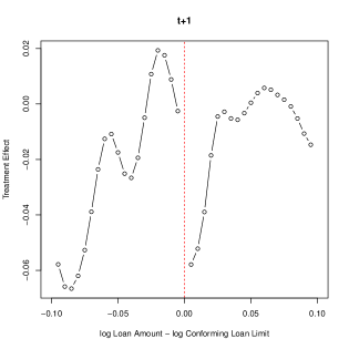
(a) Securitized Conditional on Originated, time $t+1$

(b) Securitized Conditional on Originated, time $t+2$

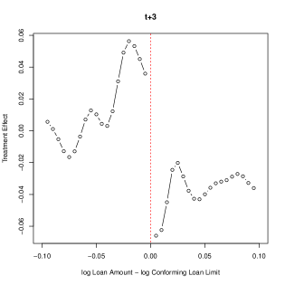
(c) Securitized Conditional on Originated, time $t+3$

(d) Securitized Conditional on Originated, time $t+4$

Open source code available at this link.

Figure 11: Would a Geographic Pricing of G-Fees Imply Redlining? First Street Risk Factor and Zip-Level Demographics

These four figures display census demographics at the ZIP level against the average ZIP-level First Street Flood Risk Score. Demographics from the 2020 Census accessed through the National Historical Geographic Information System of the University of Minnesota. Each code indicates the corresponding Census table. Each plot is binned using 40 quantiles of the risk score.

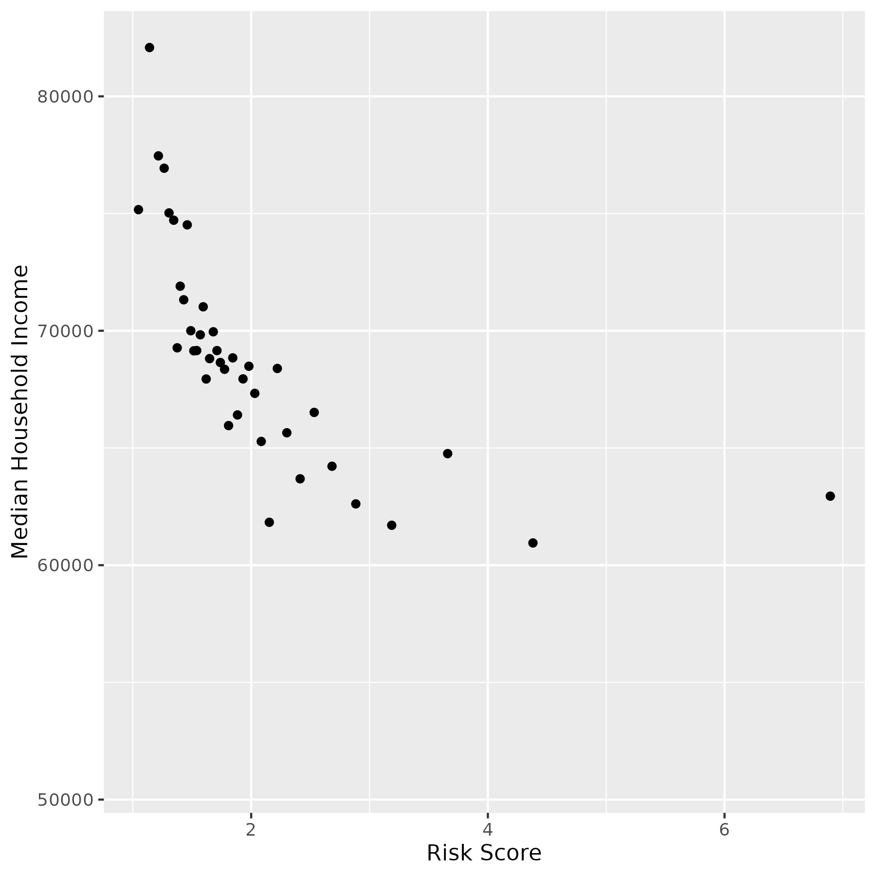
(a) Household Income (AMR8E001)

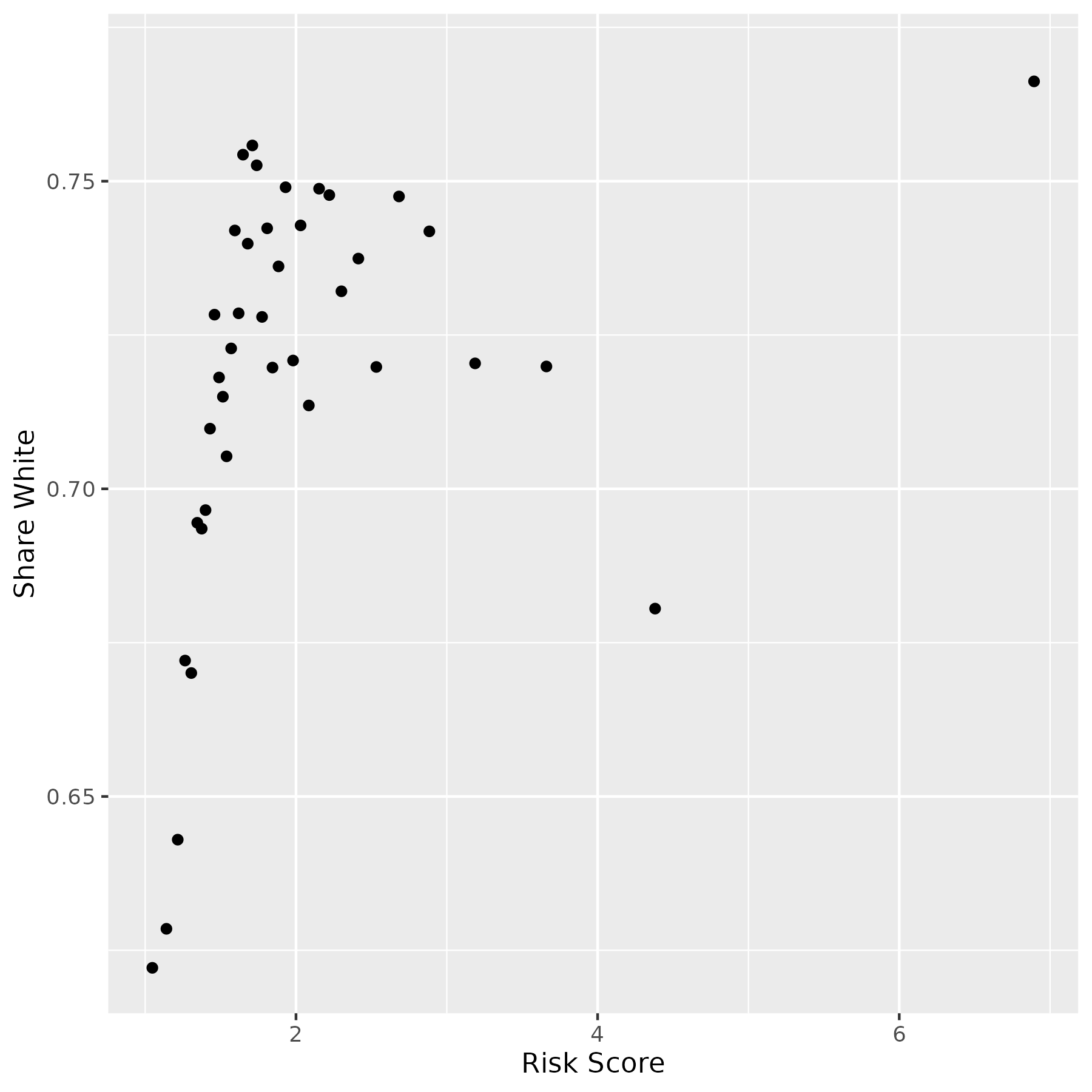
(b) Share White (B02001)

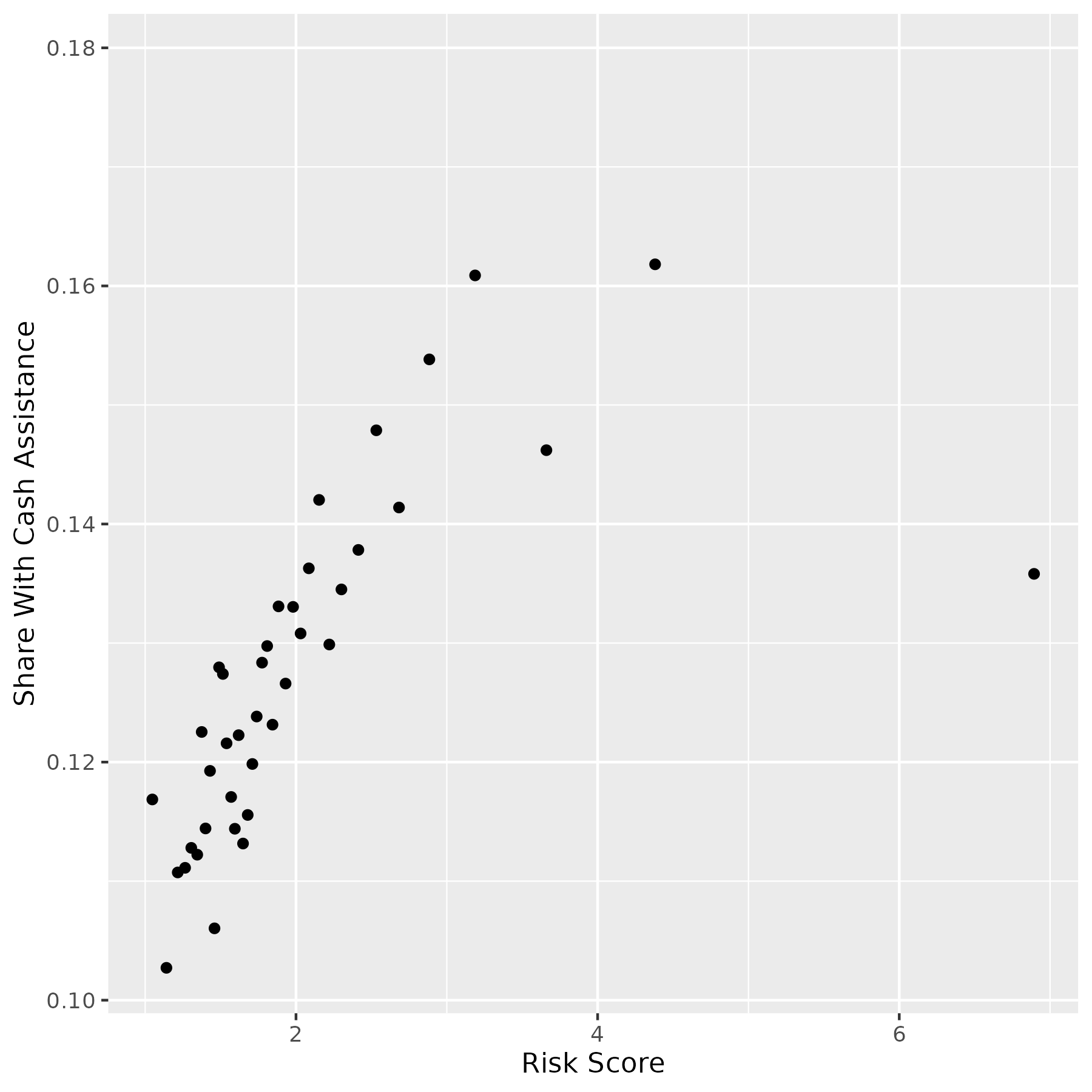
(c) Share on Cash Public Assistance or Food Stamps/SNAP (B19058)

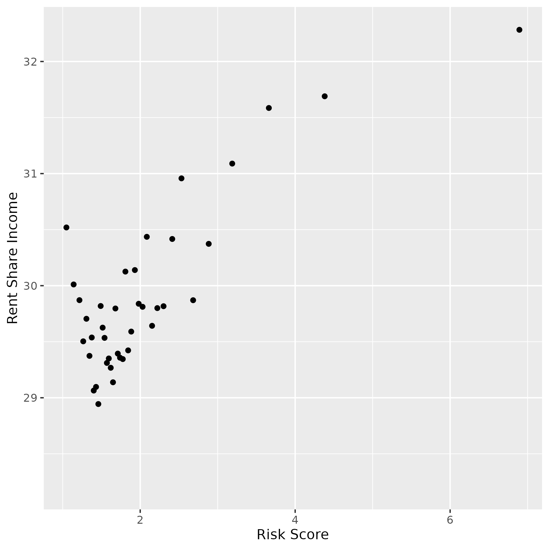
(d) Rent as Share of Household Income (B25071)

Table 5: Regression Discontinuity Estimate of the Impact of Billion-Dollar Disasters on Approval Probabilities

Dependent Variable:	Approved = 0,1
Bandwidth:	$\pm 1\%$	$\pm 2\%$	$\pm 3\%$	$\pm 4\%$
Treated $\times$ Time 0	-0.0195∗∗	-0.0213∗∗	-0.0209∗	-0.0198∗
	(0.0084)	(0.0098)	(0.0102)	(0.0101)
Treated $\times$ Time +1	-0.0507∗∗∗	-0.0486∗∗∗	-0.0455∗∗∗	-0.0432∗∗∗
	(0.0111)	(0.0105)	(0.0109)	(0.0111)
Treated $\times$ Time +2	-0.0598∗∗	-0.0596∗∗∗	-0.0575∗∗∗	-0.0548∗∗∗
	(0.0220)	(0.0156)	(0.0141)	(0.0136)
Treated $\times$ Time +3	-0.0755∗∗	-0.0719∗∗	-0.0717∗∗∗	-0.0731∗∗∗
	(0.0300)	(0.0245)	(0.0232)	(0.0225)
Treated $\times$ Time +4	-0.0565	-0.0478	-0.0457	-0.0451
	(0.0461)	(0.0383)	(0.0337)	(0.0303)
Treated $\times$ Time 0 $\times$ Below Limit	-0.0037	0.0011	0.0027	0.0028
	(0.0141)	(0.0115)	(0.0101)	(0.0096)
Treated $\times$ Time 1 $\times$ Below Limit	0.0383∗∗	0.0348∗∗∗	0.0300∗∗∗	0.0268∗∗∗
	(0.0149)	(0.0080)	(0.0061)	(0.0067)
Treated $\times$ Time 2 $\times$ Below Limit	0.0526∗	0.0501∗∗∗	0.0425∗∗∗	0.0360∗∗∗
	(0.0275)	(0.0162)	(0.0117)	(0.0100)
Treated $\times$ Time 3 $\times$ Below Limit	0.0648∗∗	0.0609∗∗∗	0.0583∗∗∗	0.0570∗∗∗
	(0.0270)	(0.0188)	(0.0160)	(0.0146)
Treated $\times$ Time 4 $\times$ Below Limit	0.0208	0.0264	0.0284	0.0291
	(0.0430)	(0.0351)	(0.0297)	(0.0259)
Year $\times$ Below Limit	Yes	Yes	Yes	Yes
Zip $\times$ Below Limit	Yes	Yes	Yes	Yes
Disaster $\times$ Below Limit	Yes	Yes	Yes	Yes
Observations	2,572,574	2,572,574	2,572,574	2,572,574
R2	0.07088	0.07076	0.06983	0.06887
Dependent Variable:	Approved = 0,1
Bandwidth:	$\pm 5\%$	$\pm 10\%$	$\pm 15\%$	$\pm 20\%$
Treated $\times$ Time 0	-0.0182∗	-0.0127	-0.0115	-0.0111
	(0.0097)	(0.0075)	(0.0067)	(0.0064)
Treated $\times$ Time +1	-0.0408∗∗∗	-0.0316∗∗∗	-0.0287∗∗∗	-0.0277∗∗∗
	(0.0107)	(0.0086)	(0.0080)	(0.0078)
Treated $\times$ Time +2	-0.0524∗∗∗	-0.0450∗∗∗	-0.0428∗∗∗	-0.0420∗∗∗
	(0.0131)	(0.0127)	(0.0133)	(0.0135)
Treated $\times$ Time +3	-0.0737∗∗∗	-0.0740∗∗∗	-0.0743∗∗∗	-0.0745∗∗∗
	(0.0218)	(0.0215)	(0.0218)	(0.0220)
Treated $\times$ Time +4	-0.0442	-0.0396	-0.0384	-0.0381
	(0.0281)	(0.0252)	(0.0249)	(0.0249)
Treated $\times$ Time 0 $\times$ Below Limit	0.0022	-0.0019	-0.0036	-0.0042
	(0.0089)	(0.0062)	(0.0054)	(0.0051)
Treated $\times$ Time 1 $\times$ Below Limit	0.0242∗∗∗	0.0140∗∗	0.0103∗	0.0088
	(0.0066)	(0.0056)	(0.0055)	(0.0056)
Treated $\times$ Time 2 $\times$ Below Limit	0.0310∗∗∗	0.0176∗∗∗	0.0134∗∗∗	0.0118∗∗
	(0.0087)	(0.0047)	(0.0045)	(0.0048)
Treated $\times$ Time 3 $\times$ Below Limit	0.0553∗∗∗	0.0465∗∗∗	0.0428∗∗∗	0.0413∗∗∗
	(0.0136)	(0.0105)	(0.0094)	(0.0090)
Treated $\times$ Time 4 $\times$ Below Limit	0.0289	0.0256	0.0241	0.0236
	(0.0234)	(0.0194)	(0.0186)	(0.0183)
Year $\times$ Below Limit	Yes	Yes	Yes	Yes
Zip $\times$ Below Limit	Yes	Yes	Yes	Yes
Disaster $\times$ Below Limit	Yes	Yes	Yes	Yes
Observations	2,572,574	2,572,574	2,572,574	2,572,574
R2	0.06790	0.06482	0.06413	0.06398
Clustered (ZCTA5CE10 & year) standard-errors in parentheses
Signif. Codes: ***: 0.01, **: 0.05, *: 0.1

Table 6: Regression Discontinuity Estimate of the Impact of Billion-Dollar Disasters on Origination Probabilities

Dependent Variable:	Originated = 0,1
Bandwidth:	$\pm 1\%$	$\pm 2\%$	$\pm 3\%$	$\pm 4\%$
Treated $\times$ Time 0	-0.0153	-0.0204	-0.0211	-0.0202
	(0.0146)	(0.0136)	(0.0128)	(0.0124)
Treated $\times$ Time +1	-0.0655∗∗∗	-0.0627∗∗∗	-0.0568∗∗∗	-0.0527∗∗∗
	(0.0155)	(0.0114)	(0.0094)	(0.0091)
Treated $\times$ Time +2	-0.0491	-0.0649∗∗∗	-0.0665∗∗∗	-0.0653∗∗∗
	(0.0336)	(0.0176)	(0.0135)	(0.0131)
Treated $\times$ Time +3	-0.0700∗∗	-0.0848∗∗	-0.0869∗∗	-0.0891∗∗∗
	(0.0328)	(0.0325)	(0.0311)	(0.0301)
Treated $\times$ Time +4	-0.0431	-0.0455	-0.0477	-0.0488
	(0.0532)	(0.0491)	(0.0436)	(0.0385)
Treated $\times$ Time 0 $\times$ Below Limit	-0.0135	-0.0021	0.0027	0.0039
	(0.0258)	(0.0215)	(0.0177)	(0.0155)
Treated $\times$ Time 1 $\times$ Below Limit	0.0457	0.0427∗∗	0.0356∗∗	0.0304∗∗
	(0.0261)	(0.0177)	(0.0125)	(0.0106)
Treated $\times$ Time 2 $\times$ Below Limit	0.0246	0.0408	0.0393∗∗	0.0349∗∗
	(0.0434)	(0.0244)	(0.0171)	(0.0143)
Treated $\times$ Time 3 $\times$ Below Limit	0.0501	0.0607∗∗	0.0608∗∗	0.0604∗∗∗
	(0.0320)	(0.0262)	(0.0218)	(0.0194)
Treated $\times$ Time 4 $\times$ Below Limit	-0.0083	0.0060	0.0140	0.0177
	(0.0508)	(0.0432)	(0.0355)	(0.0290)
Year $\times$ Below Limit	Yes	Yes	Yes	Yes
Zip $\times$ Below Limit	Yes	Yes	Yes	Yes
Disaster $\times$ Below Limit	Yes	Yes	Yes	Yes
Observations	2,572,574	2,572,574	2,572,574	2,572,574
R2	0.06821	0.06919	0.06900	0.06849
Dependent Variable:	Originated = 0,1
Bandwidth:	$\pm 5\%$	$\pm 10\%$	$\pm 15\%$	$\pm 20\%$
Variables
Treated $\times$ Time 0	-0.0186	-0.0114	-0.0089	-0.0079
	(0.0120)	(0.0087)	(0.0072)	(0.0066)
Treated $\times$ Time +1	-0.0495∗∗∗	-0.0382∗∗∗	-0.0341∗∗∗	-0.0325∗∗∗
	(0.0088)	(0.0073)	(0.0070)	(0.0070)
Treated $\times$ Time +2	-0.0641∗∗∗	-0.0611∗∗∗	-0.0601∗∗∗	-0.0598∗∗∗
	(0.0131)	(0.0138)	(0.0146)	(0.0149)
Treated $\times$ Time +3	-0.0901∗∗∗	-0.0903∗∗∗	-0.0907∗∗∗	-0.0909∗∗∗
	(0.0292)	(0.0282)	(0.0283)	(0.0284)
Treated $\times$ Time +4	-0.0480	-0.0396	-0.0362	-0.0350
	(0.0348)	(0.0281)	(0.0268)	(0.0264)
Treated $\times$ Time 0 $\times$ Below Limit	0.0036	-0.0022	-0.0052	-0.0065
	(0.0140)	(0.0091)	(0.0077)	(0.0073)
Treated $\times$ Time 1 $\times$ Below Limit	0.0267∗∗	0.0143	0.0095	0.0075
	(0.0100)	(0.0085)	(0.0086)	(0.0088)
Treated $\times$ Time 2 $\times$ Below Limit	0.0312∗∗	0.0230∗∗	0.0207∗∗	0.0199∗∗
	(0.0132)	(0.0097)	(0.0090)	(0.0091)
Treated $\times$ Time 3 $\times$ Below Limit	0.0586∗∗∗	0.0483∗∗∗	0.0446∗∗	0.0432∗∗
	(0.0177)	(0.0151)	(0.0152)	(0.0154)
Treated $\times$ Time 4 $\times$ Below Limit	0.0184	0.0115	0.0069	0.0048
	(0.0244)	(0.0156)	(0.0140)	(0.0136)
Year $\times$ Below Limit	Yes	Yes	Yes	Yes
Zip $\times$ Below Limit	Yes	Yes	Yes	Yes
Disaster $\times$ Below Limit	Yes	Yes	Yes	Yes
Observations	2,572,574	2,572,574	2,572,574	2,572,574
R2	0.06785	0.06584	0.06548	0.06545
Clustered (ZCTA5CE10 & year) standard-errors in parentheses
Signif. Codes: ***: 0.01, **: 0.05, *: 0.1

Table 7: Regression Discontinuity Estimate of the Impact of Billion-Dollar Disasters on Securitization Probabilities, Conditional on Origination

Dependent Variable:	Securitized = 0,1
Bandwidth:	$\pm 1\%$	$\pm 2\%$	$\pm 3\%$	$\pm 4\%$
Treated $\times$ Time 0	-0.0183	-0.0253	-0.0290∗	-0.0296∗
	(0.0150)	(0.0149)	(0.0146)	(0.0141)
Treated $\times$ Time +1	-0.0604∗∗∗	-0.0594∗∗∗	-0.0560∗∗	-0.0506∗∗
	(0.0176)	(0.0191)	(0.0198)	(0.0197)
Treated $\times$ Time +2	-0.0572∗∗∗	-0.0483∗	-0.0436∗	-0.0384
	(0.0180)	(0.0228)	(0.0232)	(0.0227)
Treated $\times$ Time +3	-0.0594∗	-0.0671∗∗	-0.0661∗∗	-0.0627∗∗
	(0.0307)	(0.0287)	(0.0281)	(0.0277)
Treated $\times$ Time +4	-0.1310∗∗∗	-0.1272∗∗∗	-0.1199∗∗∗	-0.1116∗∗∗
	(0.0438)	(0.0316)	(0.0285)	(0.0269)
Treated $\times$ Time 0 $\times$ Below Limit	0.0083	0.0193	0.0208	0.0193
	(0.0292)	(0.0232)	(0.0183)	(0.0155)
Treated $\times$ Time 1 $\times$ Below Limit	0.0466	0.0567∗	0.0496	0.0398
	(0.0314)	(0.0309)	(0.0299)	(0.0288)
Treated $\times$ Time 2 $\times$ Below Limit	0.0342	0.0290	0.0202	0.0118
	(0.0234)	(0.0259)	(0.0268)	(0.0269)
Treated $\times$ Time 3 $\times$ Below Limit	0.0872∗∗	0.1042∗∗∗	0.1002∗∗∗	0.0933∗∗∗
	(0.0372)	(0.0262)	(0.0249)	(0.0246)
Treated $\times$ Time 4 $\times$ Below Limit	0.1663∗∗∗	0.1773∗∗∗	0.1688∗∗∗	0.1583∗∗∗
	(0.0440)	(0.0413)	(0.0418)	(0.0432)
Year $\times$ Below Limit	Yes	Yes	Yes	Yes
Zip $\times$ Below Limit	Yes	Yes	Yes	Yes
Disaster $\times$ Below Limit	Yes	Yes	Yes	Yes
Observations	2,049,035	2,049,035	2,049,035	2,049,035
R2	0.06641	0.07239	0.07727	0.08178
Dependent Variable:	Securitized = 0,1
Bandwidth:	$\pm 5\%$	$\pm 10\%$	$\pm 15\%$	$\pm 20\%$
Treated $\times$ Time 0	-0.0292∗∗	-0.0271∗	-0.0263	-0.0259
	(0.0136)	(0.0147)	(0.0158)	(0.0163)
Treated $\times$ Time +1	-0.0456∗∗	-0.0340∗	-0.0309	-0.0297
	(0.0192)	(0.0187)	(0.0192)	(0.0195)
Treated $\times$ Time +2	-0.0342	-0.0270	-0.0254	-0.0249
	(0.0222)	(0.0221)	(0.0225)	(0.0226)
Treated $\times$ Time +3	-0.0594∗∗	-0.0520∗	-0.0501∗	-0.0494∗
	(0.0273)	(0.0273)	(0.0277)	(0.0279)
Treated $\times$ Time +4	-0.1045∗∗∗	-0.0882∗∗∗	-0.0830∗∗∗	-0.0809∗∗
	(0.0262)	(0.0267)	(0.0274)	(0.0277)
Treated $\times$ Time 0 $\times$ Below Limit	0.0174	0.0125	0.0117	0.0115
	(0.0136)	(0.0117)	(0.0121)	(0.0124)
Treated $\times$ Time 1 $\times$ Below Limit	0.0313	0.0157	0.0139	0.0136
	(0.0273)	(0.0226)	(0.0216)	(0.0214)
Treated $\times$ Time 2 $\times$ Below Limit	0.0057	-0.0024	-0.0027	-0.0027
	(0.0267)	(0.0243)	(0.0229)	(0.0224)
Treated $\times$ Time 3 $\times$ Below Limit	0.0867∗∗∗	0.0688∗∗	0.0638∗∗	0.0621∗∗
	(0.0246)	(0.0263)	(0.0276)	(0.0282)
Treated $\times$ Time 4 $\times$ Below Limit	0.1487∗∗∗	0.1226∗∗	0.1146∗∗	0.1115∗
	(0.0448)	(0.0502)	(0.0523)	(0.0532)
Year $\times$ Below Limit	Yes	Yes	Yes	Yes
Zip $\times$ Below Limit	Yes	Yes	Yes	Yes
Disaster $\times$ Below Limit	Yes	Yes	Yes	Yes
Observations	2,049,035	2,049,035	2,049,035	2,049,035
R2	0.08595	0.09977	0.10505	0.10724
Clustered (ZCTA5CE10 & year) standard-errors in parentheses
Signif. Codes: ***: 0.01, **: 0.05, *: 0.1

References

- [1] \harvarditem[Aaronson et al.]Aaronson, Hartley \harvardand Mazumder2021aaronson2021effects Aaronson, D., Hartley, D. \harvardand Mazumder, B. \harvardyearleft2021\harvardyearright, ‘The effects of the 1930s holc" redlining" maps’, American Economic Journal: Economic Policy 13(4), 355–92.
- [2] \harvarditem[Alekseev et al.]Alekseev, Giglio, Maingi, Selgrad \harvardand Stroebel2022alekseev2022quantity Alekseev, G., Giglio, S., Maingi, Q., Selgrad, J. \harvardand Stroebel, J. \harvardyearleft2022\harvardyearright, A quantity-based approach to constructing climate risk hedge portfolios, Technical report, National Bureau of Economic Research.
- [3] \harvarditemAngrist \harvardand Pischke2010angrist2010credibility Angrist, J. D. \harvardand Pischke, J.-S. \harvardyearleft2010\harvardyearright, ‘The credibility revolution in empirical economics: How better research design is taking the con out of econometrics’, Journal of economic perspectives 24(2), 3–30.
- [4] \harvarditem[Baker et al.]Baker, Bloom \harvardand Terry2020baker2020using Baker, S. R., Bloom, N. \harvardand Terry, S. J. \harvardyearleft2020\harvardyearright, Using disasters to estimate the impact of uncertainty, Technical report, National Bureau of Economic Research.
- [5] \harvarditem[Bakkensen et al.]Bakkensen, Phan \harvardand Wong2023bakkensen2023leveraging Bakkensen, L., Phan, T. \harvardand Wong, R. \harvardyearleft2023\harvardyearright, ‘Leveraging the disagreement on climate change: Theory and evidence’.
- [6] \harvarditem[Barone-Adesi et al.]Barone-Adesi, Engle, Mancini et al.2008barone2008garch Barone-Adesi, G., Engle, R. F., Mancini, L. et al. \harvardyearleft2008\harvardyearright, ‘A garch option pricing model in incomplete markets’, Review of Financial Studies 21(3), 1223–1258.
- [7] \harvarditemBhutta \harvardand Keys2022bhutta2022moral Bhutta, N. \harvardand Keys, B. J. \harvardyearleft2022\harvardyearright, ‘Moral hazard during the housing boom: Evidence from private mortgage insurance’, The Review of Financial Studies 35(2), 771–813.
- [8] \harvarditem[Biswas et al.]Biswas, Hossain \harvardand Zink2023biswas2023california Biswas, S., Hossain, M. \harvardand Zink, D. \harvardyearleft2023\harvardyearright, ‘California wildfires, property damage, and mortgage repayment’.
- [9] \harvarditem[Boustan et al.]Boustan, Kahn, Rhode \harvardand Yanguas2020boustan2020effect Boustan, L. P., Kahn, M. E., Rhode, P. W. \harvardand Yanguas, M. L. \harvardyearleft2020\harvardyearright, ‘The effect of natural disasters on economic activity in us counties: A century of data’, Journal of Urban Economics 118, 103257.
- [10] \harvarditemBrenner \harvardand Izhakian2018brenner2018asset Brenner, M. \harvardand Izhakian, Y. \harvardyearleft2018\harvardyearright, ‘Asset pricing and ambiguity: Empirical evidence’, Journal of Financial Economics 130(3), 503–531.
- [11] \harvarditemCalabria2023calabria2023shelter Calabria, M. \harvardyearleft2023\harvardyearright, Shelter from the Storm: How a COVID Mortgage Meltdown Was Averted, Cato Institute.
- [12] \harvarditemCallaway \harvardand Sant’Anna2021callaway2021difference Callaway, B. \harvardand Sant’Anna, P. H. \harvardyearleft2021\harvardyearright, ‘Difference-in-differences with multiple time periods’, Journal of Econometrics 225(2), 200–230.
- [13] \harvarditem[Cameron et al.]Cameron, Gelbach \harvardand Miller2008cameron2008bootstrap Cameron, A. C., Gelbach, J. B. \harvardand Miller, D. L. \harvardyearleft2008\harvardyearright, ‘Bootstrap-based improvements for inference with clustered errors’, The Review of Economics and Statistics 90(3), 414–427.
- [14] \harvarditemCard \harvardand Shore-Sheppard2004card2004using Card, D. \harvardand Shore-Sheppard, L. D. \harvardyearleft2004\harvardyearright, ‘Using discontinuous eligibility rules to identify the effects of the federal medicaid expansions on low-income children’, Review of Economics and Statistics 86(3), 752–766.
- [15] \harvarditemCattaneo \harvardand Titiunik2022cattaneo2022regression Cattaneo, M. D. \harvardand Titiunik, R. \harvardyearleft2022\harvardyearright, ‘Regression discontinuity designs’, Annual Review of Economics 14, 821–851.
- [16] \harvarditem[Cellini et al.]Cellini, Ferreira \harvardand Rothstein2010cellini2010value Cellini, S. R., Ferreira, F. \harvardand Rothstein, J. \harvardyearleft2010\harvardyearright, ‘The value of school facility investments: Evidence from a dynamic regression discontinuity design’, The Quarterly Journal of Economics 125(1), 215–261.
- [17] \harvarditemChamberlain1980chamberlain1980analysis Chamberlain, G. \harvardyearleft1980\harvardyearright, ‘Analysis of covariance with qualitative data’, The review of economic studies 47(1), 225–238.
- [18] \harvarditem[Cohen et al.]Cohen, Barr \harvardand Kim2021cohen2021storm Cohen, J. P., Barr, J. \harvardand Kim, E. \harvardyearleft2021\harvardyearright, ‘Storm surges, informational shocks, and the price of urban real estate: An application to the case of hurricane sandy’, Regional Science and Urban Economics 90, 103694.
- [19] \harvarditem[Connor et al.]Connor, Hagmann \harvardand Linton2012connor2012efficient Connor, G., Hagmann, M. \harvardand Linton, O. \harvardyearleft2012\harvardyearright, ‘Efficient semiparametric estimation of the fama–french model and extensions’, Econometrica 80(2), 713–754.
- [20] \harvarditemDe Chaisemartin \harvardand d’Haultfoeuille2020de2020two De Chaisemartin, C. \harvardand d’Haultfoeuille, X. \harvardyearleft2020\harvardyearright, ‘Two-way fixed effects estimators with heterogeneous treatment effects’, American Economic Review 110(9), 2964–2996.
- [21] \harvarditemdeRitis \harvardand Zandi2014deritis2014general deRitis, C. \harvardand Zandi, M. \harvardyearleft2014\harvardyearright, ‘A general theory of g-fees’, Economic and Consumer Credit Analytics .
- [22] \harvarditem[Deryugina et al.]Deryugina, Kawano \harvardand Levitt2018deryugina2018economic Deryugina, T., Kawano, L. \harvardand Levitt, S. \harvardyearleft2018\harvardyearright, ‘The economic impact of hurricane katrina on its victims: Evidence from individual tax returns’, American Economic Journal: Applied Economics 10(2), 202–233.
- [23] \harvarditem[DiNardo et al.]DiNardo, Fortin \harvardand Lemieux1996dinardo1996labor DiNardo, J., Fortin, N. M. \harvardand Lemieux, T. \harvardyearleft1996\harvardyearright, ‘Labor market institutions and the distribution of wages, 1973-1992: A semiparametric approach’, Econometrica 64(5), 1001–1044.
- [24] \harvarditemDiNardo \harvardand Lee2004dinardo2004economic DiNardo, J. \harvardand Lee, D. S. \harvardyearleft2004\harvardyearright, ‘Economic impacts of new unionization on private sector employers: 1984–2001’, The quarterly journal of economics 119(4), 1383–1441.
- [25] \harvarditem[Duclos et al.]Duclos, Esteban \harvardand Ray2004duclos2004polarization Duclos, J.-Y., Esteban, J. \harvardand Ray, D. \harvardyearleft2004\harvardyearright, ‘Polarization: concepts, measurement, estimation’, Econometrica 72(6), 1737–1772.
- [26] \harvarditem[Duffie et al.]Duffie, Gârleanu \harvardand Pedersen2005duffie2005over Duffie, D., Gârleanu, N. \harvardand Pedersen, L. H. \harvardyearleft2005\harvardyearright, ‘Over-the-counter markets’, Econometrica 73(6), 1815–1847.
- [27] \harvarditemEhrlich \harvardand Becker1972ehrlich1972market Ehrlich, I. \harvardand Becker, G. S. \harvardyearleft1972\harvardyearright, ‘Market insurance, self-insurance, and self-protection’, Journal of political Economy 80(4), 623–648.
- [28] \harvarditem[Einav et al.]Einav, Finkelstein, Ryan, Schrimpf \harvardand Cullen2013einav2013selection Einav, L., Finkelstein, A., Ryan, S. P., Schrimpf, P. \harvardand Cullen, M. R. \harvardyearleft2013\harvardyearright, ‘Selection on moral hazard in health insurance’, American Economic Review 103(1), 178–219.
- [29] \harvarditem[Elenev et al.]Elenev, Landvoigt \harvardand Van Nieuwerburgh2016elenev2016phasing Elenev, V., Landvoigt, T. \harvardand Van Nieuwerburgh, S. \harvardyearleft2016\harvardyearright, ‘Phasing out the gses’, Journal of Monetary Economics 81, 111–132.
- [30] \harvarditem[Fishback et al.]Fishback, Rose, Snowden \harvardand Storrs2022fishback2022new Fishback, P., Rose, J., Snowden, K. A. \harvardand Storrs, T. \harvardyearleft2022\harvardyearright, ‘New evidence on redlining by federal housing programs in the 1930s’, Journal of Urban Economics p. 103462.
- [31] \harvarditem[Fishback et al.]Fishback, LaVoice, Shertzer \harvardand Walsh2020fishback2020race Fishback, P. V., LaVoice, J., Shertzer, A. \harvardand Walsh, R. \harvardyearleft2020\harvardyearright, Race, risk, and the emergence of federal redlining, number w28146, National Bureau of Economic Research.
- [32] \harvarditemGanong \harvardand Noel2023ganong2023borrowers Ganong, P. \harvardand Noel, P. \harvardyearleft2023\harvardyearright, ‘Why do borrowers default on mortgages?’, The Quarterly Journal of Economics 138(2), 1001–1065.
- [33] \harvarditemGeanakoplos2010geanakoplos2010leverage Geanakoplos, J. \harvardyearleft2010\harvardyearright, ‘The leverage cycle’, NBER macroeconomics annual 24(1), 1–66.
- [34] \harvarditem[Gerardi et al.]Gerardi, Rosenblatt, Willen \harvardand Yao2015gerardi2015foreclosure Gerardi, K., Rosenblatt, E., Willen, P. S. \harvardand Yao, V. \harvardyearleft2015\harvardyearright, ‘Foreclosure externalities: New evidence’, Journal of Urban Economics 87, 42–56.
- [35] \harvarditemGete \harvardand Tsouderou2022gete2022climate Gete, P. \harvardand Tsouderou, A. \harvardyearleft2022\harvardyearright, ‘Climate risk and mortgage markets: Evidence from hurricanes harvey and irma’, Available at SSRN 3961832 .
- [36] \harvarditem[Goldsmith-Pinkham et al.]Goldsmith-Pinkham, Gustafson, Lewis \harvardand Schwert2022goldsmith2022sea Goldsmith-Pinkham, P., Gustafson, M. T., Lewis, R. C. \harvardand Schwert, M. \harvardyearleft2022\harvardyearright, Sea level rise exposure and municipal bond yields, Technical report, National Bureau of Economic Research.
- [37] \harvarditemHealy \harvardand Malhotra2009healy2009myopic Healy, A. \harvardand Malhotra, N. \harvardyearleft2009\harvardyearright, ‘Myopic voters and natural disaster policy’, American Political Science Review 103(3), 387–406.
- [38] \harvarditemHeckman \harvardand Honore1990heckman1990empirical Heckman, J. J. \harvardand Honore, B. E. \harvardyearleft1990\harvardyearright, ‘The empirical content of the roy model’, Econometrica: Journal of the Econometric Society pp. 1121–1149.
- [39] \harvarditem[Hertzberg et al.]Hertzberg, Liberman \harvardand Paravisini2016hertzberg2016adverse Hertzberg, A., Liberman, A. \harvardand Paravisini, D. \harvardyearleft2016\harvardyearright, ‘Adverse selection on maturity: Evidence from online consumer credit?’.
- [40] \harvarditem[Ho et al.]Ho, Huynh, Jacho-Chávez \harvardand Vallée2023ho2023we Ho, A. T., Huynh, K. P., Jacho-Chávez, D. T. \harvardand Vallée, G. \harvardyearleft2023\harvardyearright, ‘We didn’t start the fire: Effects of a natural disaster on consumers’ financial distress’, Journal of Environmental Economics and Management 119, 102790.
- [41] \harvarditem[Holtermans et al.]Holtermans, Kahn \harvardand Kok2022holtermans2022climate Holtermans, R., Kahn, M. E. \harvardand Kok, N. \harvardyearleft2022\harvardyearright, ‘Climate risk and commercial mortgage delinquency’, MIT Center for Real Estate Research Paper (22/04).
- [42] \harvarditemImbens \harvardand Lemieux2008imbens2008regression Imbens, G. W. \harvardand Lemieux, T. \harvardyearleft2008\harvardyearright, ‘Regression discontinuity designs: A guide to practice’, Journal of econometrics 142(2), 615–635.
- [43] \harvarditem[Indaco et al.]Indaco, Ortega \harvardand Taspinar2021indaco2021hurricanes Indaco, A., Ortega, F. \harvardand Taspinar, S. \harvardyearleft2021\harvardyearright, ‘Hurricanes, flood risk and the economic adaptation of businesses’, Journal of Economic Geography 21(4), 557–591.
- [44] \harvarditem[Issler et al.]Issler, Stanton, Vergara \harvardand Wallace2021issler2021housing Issler, P., Stanton, R., Vergara, C. \harvardand Wallace, N. \harvardyearleft2021\harvardyearright, ‘Housing and mortgage markets with climate risk: Evidence from california wildfires’.
- [45] \harvarditem[Jerch et al.]Jerch, Kahn \harvardand Lin2023jerch2023local Jerch, R., Kahn, M. E. \harvardand Lin, G. C. \harvardyearleft2023\harvardyearright, ‘Local public finance dynamics and hurricane shocks’, Journal of Urban Economics 134, 103516.
- [46] \harvarditemKahn2021kahn2021adapting Kahn, M. E. \harvardyearleft2021\harvardyearright, Adapting to Climate Change, Yale University Press.
- [47] \harvarditem[Keys et al.]Keys, Mukherjee, Seru \harvardand Vig2010keys2010did Keys, B. J., Mukherjee, T., Seru, A. \harvardand Vig, V. \harvardyearleft2010\harvardyearright, ‘Did securitization lead to lax screening? evidence from subprime loans’, The Quarterly journal of economics 125(1), 307–362.
- [48] \harvarditemKeys \harvardand Mulder2020keys2020neglected Keys, B. J. \harvardand Mulder, P. \harvardyearleft2020\harvardyearright, Neglected no more: Housing markets, mortgage lending, and sea level rise, Technical report, National Bureau of Economic Research.
- [49] \harvarditemKoijen \harvardand Yogo2019koijen2019demand Koijen, R. S. \harvardand Yogo, M. \harvardyearleft2019\harvardyearright, ‘A demand system approach to asset pricing’, Journal of Political Economy 127(4), 1475–1515.
- [50] \harvarditem[LaCour-Little et al.]LaCour-Little, Pavlov \harvardand Wachter2022lacour2022adverse LaCour-Little, M., Pavlov, A. D. \harvardand Wachter, S. M. \harvardyearleft2022\harvardyearright, ‘Adverse selection and climate risk: A response to ouazad and khan (2021)’, Available at SSRN .
- [51] \harvarditemLancaster2000lancaster2000incidental Lancaster, T. \harvardyearleft2000\harvardyearright, ‘The incidental parameter problem since 1948’, Journal of econometrics 95(2), 391–413.
- [52] \harvarditemLayton2023layton2023 Layton, D. H. \harvardyearleft2023\harvardyearright, ‘Current gse guarantee fees are too low to be consistent with regulatory capital: Does this mean a large increase is coming?’, NYU Furman Center .
- [53] \harvarditemLee \harvardand Lemieux2010lee2010regression Lee, D. S. \harvardand Lemieux, T. \harvardyearleft2010\harvardyearright, ‘Regression discontinuity designs in economics’, Journal of economic literature 48(2), 281–355.
- [54] \harvarditem[Nguyen et al.]Nguyen, Ongena, Qi \harvardand Sila2022nguyen2022climate Nguyen, D. D., Ongena, S., Qi, S. \harvardand Sila, V. \harvardyearleft2022\harvardyearright, ‘Climate change risk and the cost of mortgage credit’, Review of Finance 26(6), 1509–1549.
- [55] \harvarditemOrtega \harvardand Taspinar2018ortega2018rising Ortega, F. \harvardand Taspinar, S. \harvardyearleft2018\harvardyearright, ‘Rising sea levels and sinking property values: Hurricane sandy and new york’s housing market’, Journal of Urban Economics .
- [56] \harvarditemOuazad2022aouazaddiscussion Ouazad, A. \harvardyearleft2022a\harvardyearright, ‘Discussion of “mortgage markets with climate-change risk: Evidence from wildfires in california”’.
- [57] \harvarditemOuazad2022bouazad2022investors Ouazad, A. \harvardyearleft2022b\harvardyearright, ‘Do investors hedge against green swans? option-implied risk aversion to wildfires’, arXiv preprint arXiv:2208.06930 .
- [58] \harvarditemOuazad \harvardand Kahn2022ouazad2022mortgage Ouazad, A. \harvardand Kahn, M. E. \harvardyearleft2022\harvardyearright, ‘Mortgage finance and climate change: Securitization dynamics in the aftermath of natural disasters’, The Review of Financial Studies 35(8), 3617–3665.
- [59] \harvarditem[Ratcliffe et al.]Ratcliffe, Congdon, Teles, Stanczyk \harvardand Martín2020ratcliffe2020bad Ratcliffe, C., Congdon, W., Teles, D., Stanczyk, A. \harvardand Martín, C. \harvardyearleft2020\harvardyearright, ‘From bad to worse: Natural disasters and financial health’, Journal of Housing Research 29(sup1), S25–S53.
- [60] \harvarditem[Rehse et al.]Rehse, Riordan, Rottke \harvardand Zietz2019rehse2019effects Rehse, D., Riordan, R., Rottke, N. \harvardand Zietz, J. \harvardyearleft2019\harvardyearright, ‘The effects of uncertainty on market liquidity: Evidence from hurricane sandy’, Journal of Financial Economics 134(2), 318–332.
- [61] \harvarditem[Richardson et al.]Richardson, Van Nieuwerburgh \harvardand White2017richardson2017gses Richardson, M. P., Van Nieuwerburgh, S. \harvardand White, L. J. \harvardyearleft2017\harvardyearright, ‘What to do about the gses?’, Annual Review of Financial Economics 9, 21–41.
- [62] \harvarditem[Roth et al.]Roth, Sant’Anna, Bilinski \harvardand Poe2023roth2023s Roth, J., Sant’Anna, P. H., Bilinski, A. \harvardand Poe, J. \harvardyearleft2023\harvardyearright, ‘What’s trending in difference-in-differences? a synthesis of the recent econometrics literature’, Journal of Econometrics .
- [63] \harvarditemSastry2021sastry2021bears Sastry, P. \harvardyearleft2021\harvardyearright, ‘Who bears flood risk? evidence from mortgage markets in florida’.
- [64] \harvarditem[Smith et al.]Smith, Carbone, Pope, Hallstrom \harvardand Darden2022smith2022adjusting Smith, V. K., Carbone, J. C., Pope, J. C., Hallstrom, D. G. \harvardand Darden, M. E. \harvardyearleft2022\harvardyearright, Adjusting to natural disasters, in ‘The Economics of Environmental Risk’, Edward Elgar Publishing, pp. 297–314.
- [65] \harvarditemVickery \harvardand Wright2013vickery2013tba Vickery, J. I. \harvardand Wright, J. \harvardyearleft2013\harvardyearright, ‘Tba trading and liquidity in the agency mbs market’, Economic Policy Review 19(1).
- [66]