Fast Pareto Optimization Using Sliding Window Selection

Abstract

Pareto optimization using evolutionary multi-objective algorithms has been widely applied to solve constrained submodular optimization problems. A crucial factor determining the runtime of the used evolutionary algorithms to obtain good approximations is the population size of the algorithms which grows with the number of trade-offs that the algorithms encounter. In this paper, we introduce a sliding window speed up technique for recently introduced algorithms. We prove that our technique eliminates the population size as a crucial factor negatively impacting the runtime and achieves the same theoretical performance guarantees as previous approaches within less computation time. Our experimental investigations for the classical maximum coverage problem confirms that our sliding window technique clearly leads to better results for a wide range of instances and constraint settings.

1 Introduction

Many real-world optimization problems face diminishing returns when adding additional elements to a solution and can be formulated in terms of a submodular function [1, 2]. Problems that can be stated in terms of a submodular function include classical combinatorial optimization problems such as the computation of a maximum coverage [3] or maximum cut [4] in graphs as well as regression problems arising in machine learning.

Classical approximation algorithms for monotone submodular optimization problems under different types of constraints rely on greedy approaches which select elements with the largest benefit/cost gain according to the gain with respect to the given submodular function and the additional cost with respect to the given constraint [5, 2]. During the last years, evolutionary multi-objective algorithms have been shown to provide the same theoretical worst case performance guarantees on solution quality as the greedy approaches while clearly outperforming classical greedy approximation algorithms in practice [6, 7, 8, 9]. Results are obtained by means of rigorous runtime analysis (see [10, 11] for comprehensive overviews) which is a major tool for the analysis of evolutionary algorithms.

The analyzed approaches use a 2-objective formulation of the problem where the first objective is to maximize the given submodular function and the second objective is to minimize the cost of the given constraint. The two objectives are optimized simultaneously using variants of the GSEMO algorithm [12, 13] and the algorithm outputs the feasible solution with the highest function value when terminating. Before GSEMO has been applied analyzed for submodular problems in the prescribed way, such a multi-objective set up has already been shown to be provably successful for other constrained single-objective optimization problems such as minimum spanning trees [14] and vertex and set covering problems [15, 16] through different types of runtime analyses.

A crucial factor which significantly influences the runtime of these Pareto optimization approaches using GSEMO is the size of the population that the algorithm encounters. This is in particular the case for problems where both objectives can potentially attain exponentially many different functions values. In the context of submodular optimization this is the case iff the function $f$ to be optimized as well as the constraint allow exponentially many trade-offs. In order to produce a new solution, a solution chosen uniformly at random from the current population is mutated to produce an offspring. A large population size implies that often time is wasted by not selecting the right individual for mutation.

1.1 Our contribution

In this paper, we present a sliding window approach for fast Pareto optimization called SW-GSEMO. This approach is inspired by the fact that several previous runtime analyses of GSEMO for Pareto optimization (e. g., [6, 8]) consider improving steps of a certain kind only. More precisely, they follow an inductive approach, e. g., where high-quality solutions having a cost value of $i$ in the constraint are mutated to high-quality solutions of constraint cost value $i+1$, which we call a success. (More general sequences of larger increase per success are possible and will be considered in this paper.) Steps choosing individuals of other constraint cost values do not have any benefit for the analysis. Assuming that the successes increasing the quality and cost constraint value have the same success probability (or at least the same lower bound on it), the analysis essentially considers phases of uniform length where each phase must be concluded by a success for the next phase to start. More precisely, the runtime analysis typically allocates a window of $t^{*}$ steps, for a certain number $t^{*}$ depending on the success probability, and proves that a success is for within an expected number of $t^{*}$ steps or is even highly likely in such a phase. Nevertheless, although only steps choosing individuals of constraint value $i$ are relevant for the phase, the classical GSEMO selects the individual to be mutated uniformly a random from the population, leading to the “wasted” steps as mentioned above.

Our sliding window approach replaces the uniform selection with a time-dependent window for selecting individuals based on their constraint cost value. This time-dependent window is of uniform length $T$, which is determined by the parameters of of the new algorithm, and chooses individuals with constraint cost value $i$ for $T$ steps each. In our analysis, $T$ will be at least $t^{*}$, i. e., a proven length of the phase allowing a success towards a high-quality solution of the following constraint cost value with high probability. This allows the algorithm to make time-dependent progress and to focus the search on solutions of a “beneficial” cost constraint value, which in the end results with high probability in the same approximation guarantee as the standard Pareto optimization approaches using classical GSEMO. Our analysis points out that our proven runtime bound is independent of the maximum population size that the algorithm attains during its run. The provides significantly better upper bounds for our fast Pareto optimization approach compared to previous Pareto optimization approaches.

In our experimental study, we consider a wide range of social network graphs with different types of cost constraints and investigate the classical NP-hard maximum coverage problem. We consider uniform constraints where each node has a cost of $1$ as well as random constraints where the cost are chosen uniformly at random in the interval $[0.5,1.5]$. Compared to previous studies, we examine settings that result in a much larger number of trade-offs as we investigate larger graphs in conjunction with larger constraint bound. We point out that our sliding window selection provides significantly better results for various time budgets and constraint settings. Our analysis in terms of the resulting populations shows that the sliding window approach provides a much more focused Pareto optimization approach that produces a significantly larger number of trade-offs with respect to the constraint value and the considered goal function, in our case the maximum coverage score.

The outline of the paper is as follows. In Section 2, we introduce the class of problems we consider in this paper. Section 3 presents our new SW-GSEMO algorithm. We provide our theoretical analysis of this algorithm in Section 4 and an experimental evaluation in Section 5. Finally, we finish with some concluding remarks.

2 Preliminaries

In this section, we describe the problem classes and algorithms relevant for our study. Overall, the aim is to maximize pseudo-boolean fitness/objective functions $f\colon\{0,1\}^{n}\to\mathbb{R}$ under constraints on the allowed search points. An important class of such functions is given by the so-called submodular functions [1]. We formulate it here on bit strings on length $n$; in the literature, also an equivalent formulation using subsets of a ground set $V=\{v_{1},\dots,v_{n}\}$ can be found. The notation $x\leq y$ for two bit strings $x,y\in\{0,1\}^{n}$ means that $x$ is component-wise no larger than $y$, i. e., $x_{i}\leq y_{i}$ for all $i\in\{1,\dots,n\}$.

Definition 1.

A function $f\colon\{0,1\}^{n}\to\mathbb{R}^{+}$ is called submodular if for all $x,y\in\{0,1\}^{n}$ where $x\leq y$ and all $i$ where $x_{i}=y_{i}=0$ it holds that

$$f(x\oplus e_{i})-f(x)\geq f(y\oplus e_{i})-f(x)$$

where $a\oplus e_{i}$ is the bit string obtained by setting bit $i$ of $a$ to $1$.

We will also consider functions that are monotone (either being submodular at the same time or without being submodular). A function $f\colon\{0,1\}^{n}\to\mathbb{R}$ is called monotone if for all $x,y\in\{0,1\}^{n}$ where $x\leq y$ it holds that $f(x)\leq f(y)$, i. e., setting bits to $1$ without setting existing 1-bits to $0$ will not decrease fitness.

Optimizing motonone functions becomes difficult if different constraints are introduced. Formally, there is a cost function $c\colon\{0,1\}^{n}\to\mathbb{R}$ and a budget $B\in\mathbb{R}$ that the cost has to respect. Then the general optimization problem is defined as follows.

Definition 2 (General Optimization Problem).

Given a monotone objective function $f\colon\{0,1\}^{n}\to\mathbb{R}$, a monotone cost function $c\colon\{0,1\}^{n}\to\mathbb{R}$ and a budget $B\in\mathbb{R}$, find

$$\arg\max_{x\in\{0,1\}^{n}}f(x)\text{ such that }c(x)\leq B.$$

A constraint function $c$ is called uniform if it just counts the number of one-bits in $x$, i. e., $c(x)=\sum_{i=1}^{n}x_{i}$.

In recent years, several variations of the problem in Definition 2 have been solved using multi-objective evolutionary algorithms like the classical GSEMO algorithm [6, 7, 8, 17]. In the following, we describe the basic concepts of multi-objective optimization relevant for our approach.

Let $x,y\in\{0,1\}^{n}$ be two search points. We say that $x$ (weakly) dominates y ($x\succeq y$) iff $f(x)\geq f(x)$ and $c(x)\leq c(y)$ holds. We say $x$ strictly dominates $y$ ($x\succeq y$) iff $x\succeq y$ and $(f(x)\not=f(y)\vee c(x)\not=c(y))$. The dominance relationship applies in the same way to the objective vectors $(f(x),c(x))$ of the solutions. The set of non-dominated solutions is called the Pareto set and the set of non-dominated objectice vectors is called the Pareto front.

The classical goal in multi-objective optimization is to compute for each Pareto optimal objective vector a corresponding solution. The approaches using Pareto optimization for constrained submodular problems as investigated in, e. g., [6, 8], differ from this goal. Here the multi-objective approach is used to obtain a feasible solution, i. e., a solution for which $c(x)\leq B$ holds, that has the largest possible functions value $f(x)$.

3 Sliding Window GSEMO

The classical GSEMO algorithm [12, 13] (see Algorithm 1) has been widely used in the context of Pareto optimization. As done in [8], we consider the variant starting with the search point $0^{n}$. This search point is crucial for its progress and the basis for obtaining theoretical performance guarantees. GSEMO keeps for each non-dominated objective vector obtained during the optimization run exactly one solution in its current population $P$. In each iteration one solution $x\in P$ is chosen for mutation to produce an offspring $y$. The solution $y$ is accepted and included in the population if there is no solution $z$ in the current population that strictly dominates $y$. If $y$ is accepted, then all solutions that are (weakly) dominated by $y$ are removed from $P$.

We introduce the Sliding Window GSEMO (SW-GSEMO) algorithm given in Algorithm 2. The algorithm differs from the classical GSEMO algorithm by selecting the parent $x$ that is used for mutation in a time dependent way with respect to its constraint value $c(x)$ (see the sliding-selection procedure given in Algorithm 3). Let $t_{\mathit{max}}$ be the total time that we allocate to the sliding window approach. Let $t$ the the current iteration number. If $t\leq t_{\mathit{max}}$, the we select an individual of constraint value which matches the linear time progress from $0$ to constraint bound $B$, i.e. an individual with constraint value $\hat{c}=B/t_{\mathit{max}}$. As this value might not be integral, we use the interval $[\lfloor\hat{c}\rfloor,\lceil\hat{c}\rceil]$. In the case that there is no such individual in the population, an individual is chosen uniformly at random from the whole population $P$ as done in the classical GSEMO algorithm.

For mutation we analyze standard bit mutation. Here we create $y$ by flipping each bit $x_{i}$ of $x$ with probability $\frac{1}{n}$. As standard bit mutations have a probability of roughly $1/e$ of not flipping any bit in a mutation step, we use the standard bit mutation operator plus outlined in Algorithm 4 in our experimental studies. We note that all theorectical results obtained in this paper hold for standard bit mutations and standard bit mutatations plus.

As done in the area of runtime analysis, we measure the runtime of an algorithm buy the number of fitness evaluations. We analyze the Sliding Window GSEMO algorithm with respect to the number of fitness evaluations and determine values of $t_{\mathit{max}}$ for which the algorithm has obtained good approximation with high probability, i.e. with probability $1-o(1)$. The determined values of $t_{\mathit{max}}$ in our theorems in Section 4 are significantly lower than the bounds on the expected time to obtain the same approximations by the classical GSEMO algorithm.

Set $x=0^{n}$;

$P\leftarrow\{x\}$;

repeat

       Choose $x\in P$ uniformly at random;

       Create $y$ from $x$ by mutation;

       if $\nexists\,w\in P:w\succ y$ then

             $P\leftarrow(P\setminus\{z\in P\mid y\succeq z\})\cup\{y\}$;

            

      

until $\mathit{stop}$;

Algorithm 1 Global simple evolutionary multi-objective optimizer (GSEMO)

Set $x=0^{n}$;

$P\leftarrow\{x\}$;

$t\leftarrow 0$;

repeat

       $t\leftarrow t+1$;

       Choose $x=\text{sliding-selection}(P,t,t_{\mathit{max}},B)$;

       Create $y$ from $x$ by mutation;

       if $\nexists\,w\in P:w\succ y$ then

             $P\leftarrow(P\setminus\{z\in P\mid y\succeq z\})\cup\{y\}$;

            

      

until $\mathit{t\geq t_{\mathit{max}}}$;

Algorithm 2 Sliding Window GSEMO (SW-GSEMO)

if $t\leq t_{\mathit{max}}$ then

       $\hat{c}\leftarrow(t/t_{\mathit{max}})\cdot B$;

       $\hat{P}=\{x\in P\mid\lfloor\hat{c}\rfloor-\leq c(x)\leq\lceil\hat{c}\rceil\}$;

       if $\hat{P}=\emptyset$ then

            $\hat{P}\leftarrow P$;

      

else

       $\hat{P}\leftarrow P$;

      

Choose $x\in\hat{P}$ uniformly at random;

Return $x$;

Algorithm 3 sliding-selection$(P,t,t_{\mathit{max}},B)$

$y\leftarrow x$;

repeat

       Create $y$ from $x$ by flipping each bit $x_{i}$ of $x$ with probability $\frac{1}{n}$.

until $x\not=y$;

Return $y$;

Algorithm 4 Standard-bit-mutation-plus(x)

4 Improved Runtime Bounds for SW-GSEMO

Friedrich and Neumann [6] show that the classical GESMO finds a $(1-1/e)$-approximation to a monotone submodular function under a uniform constraint of size $r$ in expected time $O(n^{2}(\log n+r))$. A factor $n$ in their analysis stems from the fact that the population of GESMO can have size up to $r\leq n$. Thanks to the sliding window approach, which only selects from a certain subset of the population, this factor $n$ does not appear in the following bound that we prove for SW-GSEMO. More precisely, the runtime guarantee in the following theorem 1 is by a factor of $\Theta(n/\!\log n)$ better if $r\geq\log$. For smaller $r$, we gain a factor of at least $\Theta(n/r)$.

Theorem 1.

Consider the SW-GSEMO with $t_{\mathit{max}}=4ern\ln n$ on a monotone submodular function $f$ under a uniform constraint of size $r$. Then with probability $1-o(1)$, the time until a $(1-1/e)$-approximation has been found is bounded from above by $t_{\mathit{max}}=O(nr\log n)$.

Proof.

We follow the proof of Theorem 2 in [6]. As in that work, the aim is to include for every $j\in\{0,\dots,r\}$ an element $x_{j}$ in the population such that

$$f(x_{j})\geq(1-(1-1/r)^{j})f(\mathrm{OPT}),$$

where $\mathrm{OPT}$ is an optimal solution. If this holds, then the element $x_{r}$ satisfies the desired approximation ratio. We also know from [6] that the probability of mutating $x_{j}$ to $x_{j+1}$ is at least $1/(en)$ since it is sufficient to insert the element yielding the largest increase of $f$ and not to flip the rest of the bits.

We now consider a sequence of events leading to the inclusion of elements $x_{j}$ in the population for growing $j$. By definition of SW-GSEMO, element $x_{0}$ is in the population at time $0$. Assume that element $x_{j}$, where $j\in\{0,\dots,r-1\}$, is in the population $P$ at time $\tau_{j}\coloneqq 4ejn\ln n$. Then, by definition of the set $\hat{P}$, it is available for selection up to time

$$\tau_{j+1}-1=4e(j+1)n\ln n-1$$

since

$$\lfloor((4e(j+1)n\ln n-1)/t_{\mathit{max}})\cdot r\rfloor=j.$$

Moreover, the size of the subset population $\hat{P}$ that the algorithm selects from is bounded from above by $2$ since $\lceil\hat{c}\rceil-\lfloor\hat{c}\rfloor\leq 1$ and there is at most one non-dominated element for every constraint value. Therefore, the probability of choosing $x_{j}$ and mutating it to $x_{j+1}$ is at least $1/(2en)$ from time $\tau_{j}$ until time $\tau_{j+1}-1$, i. e., for a period of $4en\ln n$ steps, and the probability of this not happening is at most

$$(1-1/(2en))^{4en\ln n}\leq 1/n^{2}.$$

By a union bound over the $r$ elements to be included, the probability that there is a $j\in\{1,\dots,r\}$ such that $x_{j}$ is not included by time $\tau_{j}$ is $O(1/n)$. ∎

4.1 General Cost Constraints

We will show that the sliding window approach can also be used for more general optimization problems than submodular functions and also leads to improved runtime guarantees there. Specifically, we extend the approach to cover general cost constraints similar to the scenario studied in [8]. They use GSEMO (named POMC in their work) for the optimization scenario described in Definition 2, i. e., a monotone objective function $f\colon\{0,1\}^{n}\to\mathbb{R}^{+}$ under the constraint that a monotone cost function $c\colon\{0,1\}^{n}\to\mathbb{R}^{+}$ respects a cost bound $B$.

When transferring the set-up of [8], we have introduce the following restriction: the image set of the cost function must be the positive integers, i. e., $c\colon\{0,1\}^{n}\to\mathbb{N}$. Otherwise, all cost values could be in a narrow real-valued interval so that the sliding window approach would not necessarily have any effect.

To formulate our result, we define the submodularity ratio in the same way as in earlier work (e. g., [8]).

Definition 3.

The submodularity ratio of a function $f\colon\{0,1\}^{n}\to\mathbb{R}^{+}$ with respect to a constraint $c\colon\{0,1\}^{n}\to\mathbb{N}$ is defined as

$$\alpha_{f}\coloneqq\min_{\begin{subarray}{c}x,y\in\{0,1\}^{n},i\in\{1,\dots,n\}\\ x\leq y\wedge x_{i}=y_{i}=0\end{subarray}}\frac{f(x\oplus e_{i})-f(x)}{c(y\oplus e_{i})-c(y)},$$

where $a\oplus e_{i}$ is the bit string obtained by setting bit $i$ of $a$ to $1$.

The approximation guarantee proved for GSEMO in [8] depends on $\alpha_{f}$ and the following quantity.

Definition 4.

The minimum marginal gain of a function $c\colon\{0,1\}^{n}\to\mathbb{N}$ is defined as

$$\delta_{c}=\min_{x\in\{0,1\}^{n},i\in\{1,\dots,n\},x_{i}=0}c(x\oplus e_{i})-c(x)$$

In our analysis, we shall follow the assumption from [8] that $\delta_{c}>0$, i. e., adding an element to the solution will always increase the cost value.

Theorem 2 in [8] depends on the submodularity ratio, minimum marginal gain and the maximum population size $P_{\max}$ reached by a run of GSEMO on the bi-objective function maximizing $f$ and minimizing a variant $\hat{c}$ of $c$ (explained below). It states that within $O(enBP_{\max}/\delta_{\hat{c}})$ iterations, GESMO finds a solution $x$ such that $f(x)\geq\frac{\alpha_{f}}{2}(1-1/e^{\alpha_{f}})\cdot f(\hat{x})$, where $\hat{x}$ is an optimal solution when maximizing $f$ with the original cost function $c$ but under a slightly increased budget with respect to $B$ (precisely defined in Equation (4) in [8] and further detailed in [5]). Our main result, formulated in the following theorem, is that the SW-GSEMO obtains solutions with the same quality guarantee in an expected time where the $P_{\max}$ factor does not appear. As a detail in the formulation, the algorithm can be run with an approximation $\hat{c}$ of the original cost function $c$ that is by a certain factor $\phi(n)$ larger (i. e., $c(x)\leq\hat{c}(x)\leq\phi(n)c(x)$, see [5] for details).

Theorem 2.

Consider the problem of maximizing a monotone function $f\colon\{0,1\}^{n}\to\mathbb{R}^{+}$ under a monotone approximate cost function $\hat{c}\colon\{0,1\}^{n}\to\mathbb{N}^{+}$ with constraint $B$ and apply SW-GSEMO to the objective function $(f_{1}(x),f_{2}(x)$), where $f_{2}(x)=-\hat{c}(x)$ and

$$f_{1}(x)=\begin{cases}-\infty&\text{ if $\hat{c}(x)>B$}\\ f(x)&\text{otherwise}\end{cases}.$$

If $t_{\mathit{max}}=2en(B/\delta_{\hat{c}})\ln(n+B/\delta_{\hat{c}})$, then with probability at least $1-o(1)$ a solution of quality at least $\frac{\alpha_{f}}{2}(1-1/e^{\alpha_{f}})\cdot f(\hat{x})$ is found in $t_{\mathit{max}}$ iterations, with $\delta_{\hat{c}}>0$, $\alpha_{f}$ and $\hat{x}$ as defined above.

Proof.

We follow the proof of Theorem 2 in [8] and adapt it in a similar way to SW-GSEMO as we did in the proof of Theorem 1 above. According to the analysis in [8], the approximation result is achieved by a sequence of steps choosing an individual of cost value at most $j$, where $j\in\{0,\dots,B-1\}$ (here we adapted the proof to the integrality of $\hat{c}$) and flipping a zero-bit to $1$ yielding a certain minimum increase of $f$. More precisely, denoting by $P$ the current population of SW-GSEMO, we analyze the development of the quantity

$$J_{\max}=\max\{j \leq B-1\mid\,\exists x\in P\colon\hat{c}(x)\leq j$$

$$\,\wedge\,f(x)\geq(1-(1-\tfrac{\alpha_{f}j}{Bk})^{k})\cdot f(\hat{x})\text{\, for some~{}$k$}\}.$$

Clearly, the initial value of $J_{\max}$ is $0$. According to the analysis in [8], if currently $J_{\max}=i<B$, then there is either a solution $x_{i}^{*}$ of cost $\hat{c}(x^{*}_{i})\leq i$ (note that the inequality can be strict) and a zero-bit $z_{i}^{*}$ in $x$ whose flip leads to $J_{\max}\geq i+\delta_{\hat{c}}$ (hereinafter called a successful step); or there is already a solution in the population satisfying the desired quality guarantee $\frac{\alpha_{f}}{2}(1-1/e^{\alpha_{f}})\cdot f(\hat{x})$.

We now show that $x_{i}^{*}$ is chosen and bit $z_{i}^{*}$ is flipped with high probability for each of at most $B/\delta_{\hat{c}}$ values that $i$ can take in this sequence of successful steps. To this end, note that by definition, $\hat{c}(x_{i}^{*})$ is increasing with respect to $i$. Furthermore, by definition of the set $\hat{P}$ in SW-GSEMO, element $x_{i}^{*}$ from the population is available for selection for a period of

$$2en\ln(n+B/\delta_{\hat{c}})$$

steps, more precisely between time

$$2en\hat{c}(x_{i}^{*})\ln(n+B/\delta_{\hat{c}})$$

and

$$2en(\hat{c}(x_{i}^{*})+1)\ln(n+B/\delta_{\hat{c}})-1.$$

Moreover, by the same arguments as in the proof of Theorem 1, it holds that $\lvert\hat{P}\rvert\leq 2$ for the subset population $\hat{P}$ that the algorithm selects from, so the probability of a success is at least $1/(2en)$ for each stop within the mentioned period. Therefore, the probability of not having a successful step with respect to $x_{i}^{*}$ is bounded from above by

$$(1-1/(2en))^{2en\ln(n+B/\delta_{\hat{c}})}\leq\tfrac{1}{n(B/\delta_{\hat{c}})}.$$

By a union bound over the at most $B/\delta_{\hat{c}}$ required successes, the probability of missing at least one success is at most $1/n$, so altogether the desired solution quality is achieved with probability at least $1-1/n=1-o(1)$. ∎

The results from Theorems 1 and 2 are just two examples of a runtime result following an inductive sequence of improving steps based on constraint cost value. In the literature, there are further analyses of GSEMO following a similar approach (e. g., [18]), which we believe can be transferred to our sliding window approach to yield improved runtime guarantees.

5 Experimental investigations

We now carry out experimental investigations of the new Sliding Window GSEMO approach and compare it against the standard GSEMO which has been used in many theoretical and experimental studies on submodular optimization.

5.1 Experimental setup

We consider the maximum coverage problem in graphs which is one of the best known NP-hard submmodular combinatorial optimization problems. Given an undirected graph $G=(V,E)$ with $n=|V|$ nodes, we denote by $N(v)$ the set of nodes containing $v$ and its neighbours in $G$. Each node $v$ has a cost $c(v)$ and the goal is to select a set of nodes indicated $x$ such that the number of nodes covered by $x$ given as

$$\text{Coverage}(x)=\left|\bigcup_{i=1}^{n}N(v_{i})x_{i}\right|$$

is maximized under the condition that the cost of the selected nodes does not exceed a given bound B, i. e.

$$\sum_{i=1}^{n}c(v_{i})x_{i}\leq B$$

holds.

Previous studies investigated GSEMO either considered relatively small graphs or small budgets on the constraints that only allowed a small number of trade-offs to be produced. We consider sparse graphs from the from the network data repository [19] as dense graphs are usually easy to cover with just a small number of nodes and do not pose a challenge when considering the maximum coverage problem. We use the graphs ca-CSphd, ca-GrQc, Erdos992, ca-HepPh, ca-AstroPh, ca-CondMat, which consist of $1882$, $4158$, $6100$, $11204$, $17903$, $21363$ nodes, respectively. Note, that especially the large graphs with more than $10000$ nodes are pushing the limits for both algorithms when considering the given fitness evaluation budgets.

To match our theoretical investigations for the uniform constraint, we consider the uniform setting where $c(v_{i})=1$ holds for any node $v_{i}$ in the given graph. Note that the uniform setting implies that the number of trade-offs in the two objectives is at most $B+1$. In order to investigate the behaviour of the GSEMO approaches when there are more possible trade-offs, we investigate for each graph the following random setting. For an instance in the random setting, the cost of each node $v_{i}$ is chosen independently of the other uniformly at random in the interval $[0.5,1.5]$. Note that the expected cost of each node in the random setting is $1$. This set up allows us to work with the same bounds for the uniform and random setting. We use

$$B=\log_{2}n,\sqrt{n},\lfloor n/20\rfloor,\lfloor n/10\rfloor$$

such that the bounds scale with the given number of nodes in the considered graphs. Note that for the uniform case, all costs are integers and the effective bounds are the stated bounds rounded down to the next smaller integer. We consider the performance of both algorithms when given them a budget of

$$t_{\mathit{max}}=100000,500000,1000000$$

fitness evaluations. Note, that especially for the large graphs and for the larger values of $B$ this is this pushing the limits as the fitness evaluations budgets are much less then what is stated in the upper bounds on $t_{\mathit{max}}$ in Theorems 1 and 2. For every setting, we carry out 30 independent runs. We show the coverage values obtained in Table 1. In this table, we report the mean, standard deviation and the $p$-value (with $3$ decimal places) obtained by the Mann Whitney-U test. We call a result statistically significant if the $p$-value is at most $0.05$. To gain additional insights, we present the mean final population sizes among the 30 runs for each setting in Table 2.

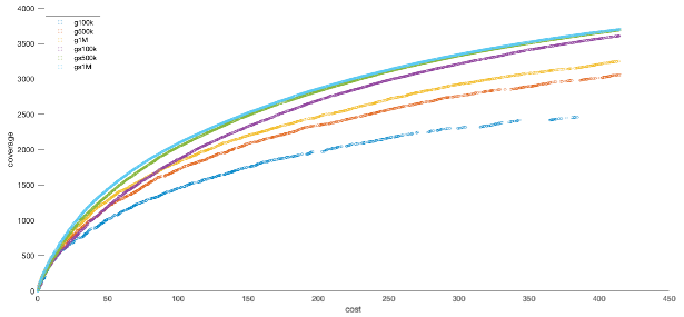
Figure 1: Example final trade-offs for the graph ca-GrQc (4158 nodes) with randomly chosen costs and budget
$B=415$ obtained by GSEMO (g) and Sliding Window GSEMO (gs) for runs with $100k$, $500k$, and $1M$ iterations.

5.2 Experimental results

The results for all considered graphs, constraint bounds, fitness evaluation budgets in the uniform and random cost setting are given in Table 1. The best results are highlighted in bold. Overall, SW-GSEMO is clearly outperforming GSEMO for almost all settings and almost all results are statistically significant. The only instances where both algorithms perform equally good are when considering the small constraint bounds of $\log_{2}n$ or $\sqrt{n}$ for ca-CSphd and $\log_{2}n$ for ca-GrQc, Erdos992, ca-HepPh. An important observation is that SW-GSEMO with only $100{,}000$ iterations is already much better than GSEMO with $1{,}000{,}000$ fitness evaluations if the constraint bound is not too small.

Considering the larger constraint bounds $\lfloor n/20\rfloor,\lfloor n/10\rfloor$ for the graphs, we can see that SW-GSEMO is significantly outperforming GSEMO. The difference in terms of coverage values between the two algorithms becomes even more pronounced when considering the random instances compared to the uniform ones. Considering the graph ca-HepPh, we can see that standard GSEMO obtains better results than SW-GSEMO when considering the constraint bound of $\log_{2}n$ in the uniform setting while SW-GSEMO is significantly outperforming GSEMO in all other settings. Looking at the results for the two largest graphs ca-AstroPh and ca-CondMat, we can see that SW-GSEMO significantly outperforms GSEMO in all considered settings.

Comparing the uniform and the random setting, we can see that the coverage values obtained by GSEMO in the random setting are much smaller than in the uniform setting when considering the three larger graphs ca-HepPh, ca-AstroPh, ca-CondMat. The only exception are some results for the small bound $B=\log_{2}n$. We attribute this deterioration of GSEMO to the larger number of trade-offs per cost unit encountered in the optimization process which significantly slows down GSEMO making progress towards the constraint bound. In contrast to this, the coverage values obtained by SW-GSEMO in the uniform and random setting when considering $t_{\mathit{max}}=500000,1000000$ are quite similar and sometimes higher for the random setting. This indicates that the sliding window selection keeps steady progress for the random setting and is not negatively impacted by the larger number of trade-offs in the random setting.

In order to better understand the performance difference between the algorithms, we examine the trade-offs produced by the algorithms. Figure 1 illustrates the final set of trade-offs for GSEMO and SW-GSEMO with respect to cost and coverage values for the different number of fitness evaluations considered. The three lower trade-off fronts depicted in blue, red, and yellow are obtaining running GSEMO with 100,000, 500,000, and 1,000,000 iterations. The three higher trade-off fronts shown in purple, green, and light blue have been obtained by SW-GSEMO in 100000, 500000, and 1000000 iterations. It can be observed that the fronts obtained by SW-GSEMO are significantly better than the ones obtained by GSEMO. The fronts for SW-GSEMO with 500000 and 1000000 iterations are very similar while the results for $100000$ are already better than the ones obtained by GSEMO with 1000000 iterations. This matches the behaviour that can already be observed for many results shown in Table 1. Furthermore, it can be seen that GSEMO has already difficulties obtaining a solution with cost close to the constraint bound when using the smallest considered budget of $100000$ fitness evaluations.

			Uniform					Random
			GSEMO		SW-GSEMO			GSEMO		SW-GSEMO
Graph	$B$	$t_{\max}$	Mean	Std	Mean	Std	$p$-value	Mean	Std	Mean	Std	$p$-value
ca-CSphd	10	100000	222	0.183	222	0.000	0.824	244	12.904	254	13.117	0.006
	10	500000	222	0.000	222	0.000	1.000	257	13.962	257	13.672	0.971
	10	1000000	222	0.000	222	0.000	1.000	258	13.938	257	13.878	0.894
	43	100000	568	5.756	599	0.730	0.000	539	13.808	625	13.711	0.000
	43	500000	600	0.254	600	0.000	0.657	615	13.150	629	13.485	0.000
	43	1000000	600	0.000	600	0.000	1.000	626	13.588	630	13.688	0.234
	94	100000	823	6.150	928	0.430	0.000	779	12.898	957	12.038	0.000
	94	500000	924	1.570	928	0.000	0.000	915	12.252	962	12.159	0.000
	94	1000000	928	0.254	928	0.000	0.657	946	11.660	963	12.173	0.000
	188	100000	1087	11.676	1280	0.814	0.000	1036	12.868	1334	12.709	0.000
	188	500000	1256	2.809	1280	0.000	0.000	1235	12.964	1341	12.718	0.000
	188	1000000	1278	1.119	1280	0.254	0.000	1291	11.671	1341	12.822	0.000
ca-GrQc	12	100000	490	8.798	505	5.701	0.000	535	17.964	595	21.765	0.000
	12	500000	509	2.539	510	0.000	0.046	601	23.067	620	20.341	0.003
	12	1000000	510	0.000	510	0.000	1.000	615	22.523	623	22.192	0.181
	64	100000	1320	15.662	1511	5.488	0.000	1281	24.326	1636	25.545	0.000
	64	500000	1490	8.904	1529	3.319	0.000	1516	25.832	1692	25.286	0.000
	64	1000000	1512	6.244	1529	2.087	0.000	1594	24.659	1699	26.351	0.000
	207	100000	2151	20.651	2748	10.797	0.000	2044	25.039	2840	23.631	0.000
	207	500000	2530	13.505	2775	3.937	0.000	2450	18.991	2918	18.449	0.000
	207	1000000	2655	9.295	2778	2.687	0.000	2600	13.956	2926	20.322	0.000
	415	100000	2704	24.887	3571	5.661	0.000	2407	51.554	3622	15.866	0.000
	415	500000	3171	13.424	3616	3.336	0.000	3047	19.085	3701	14.015	0.000
	415	1000000	3339	10.258	3622	3.468	0.000	3232	13.908	3710	12.832	0.000
Erdos992	12	100000	584	8.094	601	2.102	0.000	635	26.211	750	37.157	0.000
	12	500000	603	1.837	604	0.183	0.012	751	36.183	783	37.723	0.002
	12	1000000	604	0.254	604	0.000	0.657	774	37.049	786	38.149	0.191
	78	100000	1835	35.766	2453	6.674	0.000	1658	31.957	2512	44.639	0.000
	78	500000	2345	18.151	2472	0.791	0.000	2169	35.736	2626	44.925	0.000
	78	1000000	2438	7.439	2473	0.430	0.000	2366	41.017	2634	43.671	0.000
	305	100000	2862	54.832	4706	7.897	0.000	2547	60.705	4584	87.698	0.000
	305	500000	3824	27.333	4772	1.570	0.000	3534	30.716	4789	20.565	0.000
	305	1000000	4201	20.239	4775	0.765	0.000	3898	28.104	4799	21.492	0.000
	610	100000	3076	46.668	5251	2.343	0.000	2553	57.540	4734	464.930	0.000
	610	500000	4428	31.694	5263	0.964	0.000	4017	50.324	5376	8.230	0.000
	610	1000000	4791	22.216	5264	0.254	0.000	4516	33.380	5378	8.477	0.000
ca-HepPh	13	100000	1687	34.310	1806	30.914	0.000	1750	53.601	1979	53.815	0.000
	13	500000	1830	27.572	1844	11.761	0.019	1980	50.385	2115	48.030	0.000
	13	1000000	1854	15.539	1840	5.112	0.000	2058	50.351	2144	54.399	0.000
	105	100000	3740	48.996	4644	27.022	0.000	3598	31.674	4806	52.069	0.000
	105	500000	4309	28.317	4789	13.226	0.000	4238	40.329	5111	53.447	0.000
	105	1000000	4516	20.372	4802	10.016	0.000	4490	43.562	5176	42.558	0.000
	560	100000	5909	73.941	8544	22.516	0.000	5108	86.715	8626	40.014	0.000
	560	500000	7092	29.683	8800	11.032	0.000	6802	36.876	9058	31.968	0.000
	560	1000000	7527	24.174	8825	7.388	0.000	7249	32.562	9129	28.224	0.000
	1120	100000	5919	81.766	10196	144.717	0.000	5098	92.907	9095	1221.796	0.000
	1120	500000	8148	55.111	10494	8.483	0.000	7209	62.132	10622	45.053	0.000
	1120	1000000	8795	30.765	10523	7.263	0.000	8138	62.450	10683	30.947	0.000
ca-AstroPh	14	100000	2594	85.426	2867	57.047	0.000	2598	96.079	3026	106.242	0.000
	14	500000	2914	31.062	2974	5.396	0.000	3016	64.712	3321	80.235	0.000
	14	1000000	2962	12.480	2980	2.716	0.000	3195	77.509	3388	87.267	0.000
	133	100000	6484	77.132	8351	50.919	0.000	6221	82.193	8558	79.255	0.000
	133	500000	7551	51.042	8709	25.847	0.000	7362	61.676	9214	64.955	0.000
	133	1000000	7968	40.202	8749	14.914	0.000	7817	62.797	9372	68.257	0.000
	895	100000	9511	120.361	15033	32.462	0.000	8170	122.610	14467	1262.081	0.000
	895	500000	12360	60.272	15611	16.028	0.000	11387	100.119	15861	34.325	0.000
	895	1000000	13017	35.102	15690	11.610	0.000	12490	39.435	16014	27.498	0.000
	1790	100000	9502	97.540	16984	162.622	0.000	8137	104.415	13313	2546.964	0.000
	1790	500000	12750	88.401	17473	8.353	0.000	11374	104.602	17039	822.188	0.000
	1790	1000000	14103	54.069	17527	6.369	0.000	12743	112.303	17543	158.486	0.000
ca-CondMat	14	100000	1514	56.623	1766	44.191	0.000	1411	76.166	1759	63.903	0.000
	14	500000	1802	25.451	1854	5.063	0.000	1773	62.028	2016	79.008	0.000
	14	1000000	1846	8.628	1857	1.717	0.000	1912	69.264	2068	77.399	0.000
	146	100000	4388	71.953	6668	49.261	0.000	4106	91.413	6650	68.737	0.000
	146	500000	5585	61.992	7054	17.553	0.000	5264	65.588	7412	73.412	0.000
	146	1000000	6092	50.561	7091	8.705	0.000	5776	64.557	7560	73.139	0.000
	1068	100000	7187	130.346	15758	38.782	0.000	5779	149.352	14515	2634.382	0.000
	1068	500000	11334	67.041	16727	18.791	0.000	9655	129.937	17038	47.148	0.000
	1068	1000000	12364	69.321	16844	11.085	0.000	11533	79.858	17287	53.123	0.000
	2136	100000	7211	133.166	19120	204.254	0.000	5823	137.877	13642	3603.578	0.000
	2136	500000	11556	115.359	20093	12.913	0.000	9675	135.492	19513	1682.649	0.000
	2136	1000000	13652	84.783	20218	9.453	0.000	11632	96.193	20446	87.106	0.000

Table 1: Maximum coverage scores obtained by GSEMO and SW-GSEMO

In Table 2, we show the average number of trade-offs given by the final populations of the two algorithms for the 30 runs of each setting. We first examine the uniform setting. The budgets for our experiments are chosen small enough such that not all nodes can be covered by any solution. Therefore, in the ideal case, both algorithms would produce $B+1$ trade-offs in the uniform setting. It can be observed that this is roughly happening for the two smallest graphs ca-CSphd, ca-GrQc. For the remaining $4$ graphs, GSEMO produces significantly less points when considering the constraint bound $\lfloor n/20\rfloor,\lfloor n/10\rfloor$ while the number of trade-offs obtained by SW-GSEMO is close to $B+1$ is most uniform settings. Considering the random setting, we can see that the number of trade-offs produced by SW-GSEMO is significantly higher than for GSEMO. In the case of large graphs, the number of trade-offs produced is up to four times larger than the number of trade-offs produced by GSEMO, e.g. for graph ca-CondMat and $B=2136$. Overall this suggests that the larger number of trade-offs produced in a systematic way by the sliding window approach significantly contributes to the superior performance of SW-GSEMO.

			Uniform		Random
Graph	$B$	$t_{\max}$	G	SWG	G	SWG
ca-CSphd	10	100000	11	11	73	92
	10	500000	11	11	125	130
	10	1000000	11	11	133	132
	43	100000	44	44	172	280
	43	500000	44	44	287	435
	43	1000000	44	44	390	475
	94	100000	94	95	281	496
	94	500000	95	95	422	686
	94	1000000	95	95	540	761
	188	100000	180	189	404	785
	188	500000	189	189	591	985
	188	1000000	189	189	734	1068
ca-GrQc	12	100000	13	13	89	115
	12	500000	13	13	142	191
	12	1000000	13	13	185	236
	64	100000	65	65	261	439
	64	500000	65	65	372	700
	64	1000000	65	65	448	854
	207	100000	200	208	493	1021
	207	500000	207	208	710	1460
	207	1000000	208	208	841	1703
	415	100000	347	414	611	1500
	415	500000	400	416	967	1996
	415	1000000	409	416	1134	2246
Erdos992	12	100000	13	13	76	103
	12	500000	13	13	129	193
	12	1000000	13	13	181	251
	78	100000	78	79	237	395
	78	500000	79	79	330	684
	78	1000000	79	79	393	913
	305	100000	253	305	441	970
	305	500000	291	306	668	1497
	305	1000000	298	306	777	1885
	610	100000	296	588	440	1031
	610	500000	483	610	818	1769
	610	1000000	522	611	1014	2073
ca-HepPh	13	100000	14	14	91	118
	13	500000	14	14	125	157
	13	1000000	14	14	143	195
	105	100000	105	106	344	634
	105	500000	106	106	489	878
	105	1000000	106	106	553	1040
	560	100000	408	558	634	2083
	560	500000	521	560	1176	2849
	560	1000000	543	561	1364	3304
	1120	100000	409	1093	644	2295
	1120	500000	813	1116	1306	3854
	1120	1000000	951	1117	1718	4295
ca-AstroPh	14	100000	15	15	94	119
	14	500000	15	15	125	155
	14	1000000	15	15	142	190
	133	100000	132	134	404	808
	133	500000	134	134	565	1074
	133	1000000	134	134	663	1292
	895	100000	416	890	653	2719
	895	500000	764	895	1372	3921
	895	1000000	818	896	1755	4434
	1790	100000	413	1715	643	2237
	1790	500000	848	1767	1366	4525
	1790	1000000	1121	1776	1830	5263
ca-CondMat	14	100000	15	15	87	106
	14	500000	15	15	111	137
	14	1000000	15	15	124	166
	146	100000	144	147	410	819
	146	500000	147	147	572	1066
	146	1000000	147	147	662	1286
	1068	100000	424	1063	650	3244
	1068	500000	864	1068	1437	4953
	1068	1000000	952	1068	1929	5772
	2136	100000	425	2084	655	2801
	2136	500000	906	2125	1428	6313
	2136	1000000	1228	2131	1953	7724

Table 2: Final number of trade-off solutions obtained by GSEMO (G) and SW-GSEMO (SWG)

6 Conclusions

Pareto optimization using GSEMO has widely been applied in the context of submodular optimization. We introduced the Sliding Window GSEMO algorithm which selects an individual due to time progress and constraint value in the parent selection step. Our theoretical analysis provides better runtime bounds for SW-GSEMO while achieving the same worst-case approxmation ratios as GSEMO. Our experimental investigations for the maximum coverage problem shows that SW-GSEMO outperforms GSEMO for a wide range of settings. We also provided additional insights into the optimization process by showing that SW-GSEMO computes significantly more trade-off then GSEMO for instances with random weights or uniform instances with large budgets.

References

-
[1]
G. L. Nemhauser, L. A. Wolsey, Best
algorithms for approximating the maximum of a submodular set function,
Mathematics of Operations Research 3 (3) (1978) 177–188.
URL https://doi.org/10.1287/moor.3.3.177 - [2] A. Krause, D. Golovin, Submodular function maximization, in: Tractability: Practical approaches to hard problems, Cambridge University Press, 2014, pp. 71–104. doi:10.1017/CBO9781139177801.004.
- [3] S. Khuller, A. Moss, J. Naor, The budgeted maximum coverage problem, Information Processing Letters 70 (1) (1999) 39–45. doi:10.1016/S0020-0190(99)00031-9.
-
[4]
M. X. Goemans, D. P. Williamson,
Improved approximation
algorithms for maximum cut and satisfiability problems using semidefinite
programming, J. ACM 42 (6) (1995) 1115–1145.
doi:10.1145/227683.227684.
URL https://doi.org/10.1145/227683.227684 -
[5]
H. Zhang, Y. Vorobeychik,
Submodular
optimization with routing constraints, in: D. Schuurmans, M. P. Wellman
(Eds.), Proc. of AAAI ’16, AAAI Press, 2016, pp. 819–826.
URL http://www.aaai.org/ocs/index.php/AAAI/AAAI16/paper/view/11911 - [6] T. Friedrich, F. Neumann, Maximizing submodular functions under matroid constraints by evolutionary algorithms, Evolutionary Computation 23 (4) (2015) 543–558. doi:10.1162/EVCO_a_00159.
- [7] C. Qian, Y. Yu, Z. Zhou, Subset selection by Pareto optimization, in: Proceedings of the 28th International Conference on Neural Information Processing Systems - Volume 1, NIPS 2015, 2015, pp. 1774–1782.
-
[8]
C. Qian, J. Shi, Y. Yu, K. Tang,
On subset selection with
general cost constraints, in: C. Sierra (Ed.), Proc. of IJCAI ’17,
ijcai.org, 2017, pp. 2613–2619.
doi:10.24963/ijcai.2017/364.
URL https://doi.org/10.24963/ijcai.2017/364 - [9] A. Neumann, F. Neumann, Optimising monotone chance-constrained submodular functions using evolutionary multi-objective algorithms, in: Parallel Problem Solving from Nature, PPSN 2020, Proceedings, Part I, Vol. 12269 of LNCS, Springer, 2020, pp. 404–417. doi:10.1007/978-3-030-58112-1_28.
- [10] F. Neumann, C. Witt, Bioinspired computation in combinatorial optimization, Natural Computing Series, Springer, 2010. doi:10.1007/978-3-642-16544-3.
- [11] B. Doerr, F. Neumann, Theory of Evolutionary Computation – Recent developments in discrete optimization, Natural Computing Series, Springer, 2020. doi:10.1007/978-3-030-29414-4.
- [12] M. Laumanns, L. Thiele, E. Zitzler, Running time analysis of multiobjective evolutionary algorithms on pseudo-boolean functions, IEEE Transactions on Evolutionary Computtation 8 (2) (2004) 170–182.
- [13] O. Giel, Expected runtimes of a simple multi-objective evolutionary algorithm, in: Proc. of Congress onEvolutionary Computation (CEC’03), Vol. 3, IEEE, 2003, pp. 1918–1925.
- [14] F. Neumann, I. Wegener, Minimum spanning trees made easier via multi-objective optimization, Nat. Comput. 5 (3) (2006) 305–319.
- [15] T. Friedrich, J. He, N. Hebbinghaus, F. Neumann, C. Witt, Approximating covering problems by randomized search heuristics using multi-objective models, Evol. Comput. 18 (4) (2010) 617–633.
- [16] S. Kratsch, F. Neumann, Fixed-parameter evolutionary algorithms and the vertex cover problem, Algorithmica 65 (4) (2013) 754–771.
- [17] V. Roostapour, A. Neumann, F. Neumann, T. Friedrich, Pareto optimization for subset selection with dynamic cost constraints, Artif. Intell. 302 (2022) 103597.
-
[18]
C. Qian, D. Liu, C. Feng, K. Tang,
Multi-objective evolutionary
algorithms are generally good: Maximizing monotone submodular functions over
sequences, Theoretical Computer Science 943 (2023) 241–266.
doi:10.1016/j.tcs.2022.12.011.
URL https://doi.org/10.1016/j.tcs.2022.12.011 - [19] R. A. Rossi, N. K. Ahmed, The network data repository with interactive graph analytics and visualization, in: AAAI, AAAI Press, 2015, pp. 4292–4293.