Revealing Patterns of Symptomatology in Parkinson’s Disease: A Latent Space Analysis with 3D Convolutional Autoencoders

Abstract

This work proposes the use of 3D convolutional variational autoencoders (CVAEs) to trace the changes and symptomatology produced by neurodegeneration in Parkinson’s disease (PD). In this work, we present a novel approach to detect and quantify changes in dopamine transporter (DaT) concentration and its spatial patterns using 3D CVAEs on Ioflupane (FPCIT) imaging. Our approach leverages the power of deep learning to learn a low-dimensional representation of the brain imaging data, which then is linked to different symptom categories using regression algorithms. We demonstrate the effectiveness of our approach on a dataset of PD patients and healthy controls, and show that general symptomatology (UPDRS) is linked to a d-dimensional decomposition via the CVAE with R2>0.25. Our work shows the potential of representation learning not only in early diagnosis but in understanding neurodegeneration processes and symptomatology.

1 Introduction

Parkinson’s disease (PD) is a progressive neurodegenerative disorder that affects more than 6.2 million people worldwide [1]. PD is characterized by a loss of dopamine-producing neurons in the brain, causing tremors, stiffness, and cognitive decline among other symptoms. FPCIT (ioflupane) SPECT is the most widely extended neuroimaging technique for the diagnosis of PD. FPCIT binds to the presynaptic dopamine transporters (DaTs), allowing to visualize and quantify the DaT concentration at the striata, that characterizes PD [2]. This modality may allow to tackle one of the biggest challenges for PD: the early detection and monitoring of disease progression [3].

Recent advances in deep learning, and in particular, convolutional neural networks (CNNs) have shown promising results in medical imaging applications such as segmentation, registration, and classification [4]. Autoencoders (AEs), a type of self-supervised neural network, can learn a low-dimensional representation of high-dimensional data, making them well-suited for image compression, denoising, and anomaly detection [5].

In this paper, we propose a novel approach to detect and quantify subtle changes in DaT concentration and distribution in the brain using 3D convolutional variational AEs (CVAEs). Our approach leverages the power of deep learning to learn a low-dimensional representation of brain imaging data, which enables us to longitudinally compare images and identify patterns of change that are indicative of neurodegeneration. We demonstrate the effectiveness of our approach on a dataset of PD patients and healthy controls, and show that latent spaces can capture the variability of individual symptom categories, as well as the overall disease stage.

2 Materials and Methods

2.1 Dataset

Data for this study were obtained from the Parkinson’s Progression Markers Initiative (PPMI) database. For the most recent information on the study, please visit www.ppmi-info.org. We used the standardized “Original Cohort BL to Year 5” that includes individuals initially diagnosed as either controls (CTL) or PD affected subjects with varying levels of severity. After removing subjects with no FPCIT scans, the CTL group comprises 101 males and 53 females, while the PD group comprises 284 males and 159 females, followed for up to 5 years, with a total 1399 sessions of available data for studying the progression of imaging biomarkers and their link to PD-specific progression indicators. Symptomatology is assessed via the MDS-UPDRS scale [6], either in its aggregated form (UPDRS -total-) or its 4 parts: 1) non-motor aspects of daily living; 2) motor aspects of daily living (tremor, walking, etc); 3) motor examination (rigidity, posture, gait etc) and 4) motor complications (dyskinesia, fluctuation items).

FPCIT scans labeled as “Reconstructed” were used, having all of them a consistent orientation and similar sizes (for a scan of shape $91\times 109\times 91$). However, no spatial normalization is performed, as it was demonstrated to have small impact when using CNN architectures [4]. Intensity was normalized by substracting the background average intensity, and then dividing all voxel intensities by a non-specific reference, defined as the average voxel intensity of the cerebellum and occipital lobe. Finally, to favor convergence of the CVAE training, the upper-end values of the intensity distribution were compressed using a sigmoid function.

2.2 3D Convolutional Variational Autoencoders

An autoencoder is a neural network architecture that consists of an encoder network and a decoder network. In this work we used a 3D convolutional encoder-decoder architecture, capable of dealing with volumetric 3D images. The 3D encoder can capture spatial features at multiple scales, similarly to well-known 3D convolutional NNs [4]. Its output is a lower-dimensional representation which encodes the most salient features of the input data. Under the manifold hypothesis [5], this representation is often considered as coordinates in a “latent space” underlying the dataset. The decoder network performs the inverse operation.

Variational autoencoders consider that the latent space is indeed the parameter space of $D$ Gaussian distributions, from which the input of the decoder is sampled [7], allowing for non-sparse sampling and a quantification of uncertainty in the point estimates. The $\beta$-VAE loss function [8] was used (Equation 1):

$$\hypertarget{eq-vae}{}{\mathcal{L}_{VAE}=\mathcal{L}_{recon}+\beta\mathcal{L}_{KLD}}$$ (1)

This loss function allows controlling for the proportion of the reconstruction error and the Kullback-Leibler Divergence (KLD) (Equation 3) using the parameter $\beta$. Reconstruction error was estimated assuming that the voxel distribution among patients was guassian, which means that we could use the volumetric Mean Squared Error (MSE) (Equation 2) between the original voxel intensities $x_{j}$ and the output voxel of the decoder $\hat{x}_{j}$ for all $j$ voxels in the images. Each subject’s loss was added to conform the batch loss (reduction “sum”), which proved to improve training convergence.

$$\hypertarget{eq-recon}{}{\mathcal{L}_{recon}=\sum_{j}(x_{j}^{2}-\hat{x}_{j}^{2})}$$ (2)

$$\hypertarget{eq-kld}{}{\mathcal{L}_{KLD}=-\frac{1}{2}\sum_{i=0}^{D}\left(1+\log\sigma_{i}^{2}-\mu_{i}^{2}-\sigma_{i}^{2}\right)}$$ (3)

The specific architecture and parameters of the 3D-CVAE is shown at Table LABEL:tbl-encoder-params and Table LABEL:tbl-decoder-params. Different latent dimensionality (3, 8 and 20) was tested for 400 epochs with Adam optimizer (lr=1e-3).

Table 1: Encoder architecture parameters

Type # in # out KS Stride Padding Conv3D (1) 1 32 3 2 1 Conv3D (2) 32 64 3 2 1 Conv3D (3) 64 128 3 2 1 Conv3D (4) 128 256 3 2 1 Linear 73728 512 - - - 2 $\times$ Linear ($\mu$ and $\sigma$) 512 $D$ - - -

Table 2: Decoder architecture parameters

Type	# in	# out	KS	Stride	Padding
Linear	$D$	73728	–	–	–
ConvTranspose3d (1)	256	128	3	2	1
ConvTranspose3d (2)	128	64	3	2	1
ConvTranspose3d (3)	64	32	3	2	1
ConvTranspose3d (4)	32	1	3	2	1

2.3 Regression

The purpose of this work is to predict 4 categories of symptomatology using the latent distribution of the FPCIT image dataset. To perform such task, we explore the predictive power of two widely-used regression algorithms: Decision Trees (DT) and XGBoost. DTs are relatively simple to understand and have been widely used in medicine, because the resulting trees are directly interpretable [9]. XGboost is a scalable tree boosting system that uses approximate tree learning, and is widely extended in data science, achieving high performance in many challenges [10].

2.4 Experimental Setup

The machine learning pipeline is defined by first training the dataset and using the $\mu$ parameters of the latent distribution as features. Additionally, K-Means features (KMF), which capture the distance to a K-means cluster center, were generated to capture the salient characteristics of the data. The number of clusters used to generate KMFs is established as the maximum value between 8 and the logarithm of the dimensionality times 8, as in [11]. Then, the two regression algorithms are trained with or without these KMFs to predict the different UPDRS categories. 10-Fold cross-validation is used to compute the performance values, including the Mean Absolute Error (MAE), Root Mean Squared Error (RMSE) and coefficient of determination $R^{2}$ between the real and predicted values for UPDRS.

To more fully understand the output of the pipeline, we applied SHapley Additive exPlanations (SHAP) [12] to the outputs of each system. SHAP yields metrics such as feature importance, and the contribution of each feature to the output of the algorithm, and thus can be used to track the most relevant characteristics on the data.

3 Results and Discussion

3.1 Regression Results

The performance of the proposed regression algorithms on the 3, 8 and 20-dimensional latent space of the CVAE is shown at Figure 1. We obtained R2>0 for almost all target symptomatology categories and d-dimensional latent spaces. We can observe that, while low latent dimensionality (3, 8) is -in general- better for individual symptom categories, the details of the overall symptomatology score (UPDRS – total) is better accounted for by the 20-dimensional (20-D) CVAE, achieving a MAE = 12.21 and a R2=0.26. This speaks of the complexity of the composite, but also of its relationship to the FPCIT distribution patterns. Similarly, UPDRS 3, more dependent on measured motor symptoms, benefits from the 20-D space.

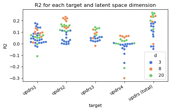
Figure 1: R2 performance for the models trained with the five symptomatology scales and 3, 8 and 20 latent-dimension.

A detailed view of the best results obtained for each combination of target scale and dimensionality of the latent space D, including their MAE, RMSE and $R^{2}$ values is shown at Table LABEL:tbl-performance.

Table 3: Classification and regression results. DT stands for Decission Trees, XGB for XG-Boost and KMF for K-Means features

target	d	model	MAE	RMSE	R2
	3	DT	3.53	4.5	0.15
updrs1	8	DT (KMF)	3.58	4.55	0.13
	20	DT (KMF)	3.69	4.71	0.07
	3	XGB (KMF)	3.96	5.23	0.11
updrs2	8	XGB (KMF)	3.68	4.86	0.23
	20	XGB (KMF)	3.74	5.08	0.16
	3	XGB (KMF)	10.78	13.11	0.06
updrs3	8	XGB (KMF)	10.21	12.93	0.09
	20	XGB (KMF)	10.03	12.59	0.14
	3	DT	0.7	1.44	0
updrs4	8	XGB	0.62	1.39	0.07
	20	DT (KMF)	0.71	1.43	0.02
	3	XGB (KMF)	13.15	16.42	0.17
updrs (total)	8	XGB	12.72	15.75	0.24
	20	XGB	12.21	15.51	0.26

3.2 Intepretability of the Space

The regression results show that there exist a predictive power in the manifold representation of the FPCIT dataset. The interpretation of the effective patterns captured by latent variables can be, in consequence, of key importance for clinical validation. While DTs (best for UPDRS 1) are visual by nature, ensemble methods such as XGBoost are more difficult to interpret. Here, SHAP can pave the way to interpret the contribution of each of the latent features to the output variables.

In this regard, the prediction of total symptomatology (UPDRS - total) is of special interest. In both the 8- and 20-dimensional spaces XGBoost achieves the largest predictive ability in terms of $R^{2}$. Consequently, the most important features -measured by SHAP- can capture the patterns that lead to this high performance. The SHAP analysis of the XGBoost regressor with the 20-dimensional space reveals the behavior shown at Figure 2.

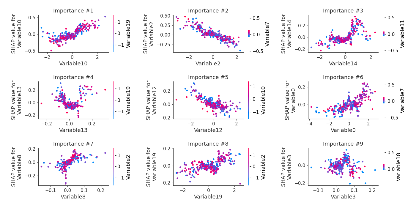
Figure 2: SHAP dependence plot of the XGBoost regressor with the 20-dimensional space

SHAP dependence plots show how the SHAP value of importance depends on a given feature, ordered from highest to lowest importance. In Figure 2 we see that the top-3 features that contribute to the output of the algorithm are variables 2, 10 and 0. Color shows the values of a second feature that may have an interaction effect with the feature we are plotting. Remember that these are the mean parameters of a Gaussian distribution that encodes the pattern for each subject. In this regard, we see an almost linear dependency between importance to the algorithm output and values of the variables, which indicates that there exist a clear relationship between them. To visualize the patterns captured by features 2 and 10, we generated brain images sampling these two features with the decoder and setting 0-mean to all other features. The result is shown at Figure 3.

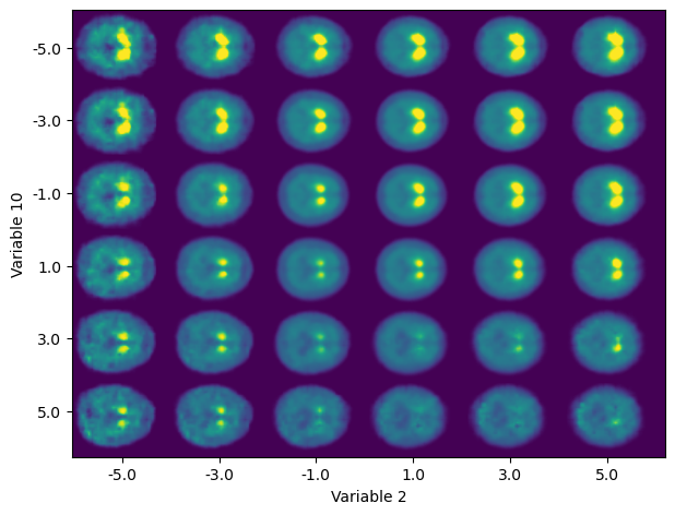
Figure 3: Latent manifold for variables 10 and 2 of the 20-dimensional latent space of the 3D CVAE.

We observe that the composition of the two variables account for two relevant characteristics of FPCIT: the overall intensity of the striata, the separation between them and the ratio between uptake at the anterior and posterior parts of the striata. General intensity and separation patterns seem to be encoded by our variable 10, whereas the striata anterior-posterior length is generally encoded by variable 2. In this regard, the overall intensity (uptake) at the striata is indeed the objective of FPCIT as a biomarker, and therefore expected. As for the anterior-posterior striata patterns, many works that used FDOPA, a presynaptic dopaminergic marker, reported a distinct anterior–posterior gradient of uptake as PD progresses [13]. This could be then a relevant marker for assessing the progression of the disease. Since SHAP importance is higher for this variable 2, we can assume that its contribution to the modelling of the progression is higher, perhaps showing a more smooth transition as the symptoms progress, in contrast to overall drug uptake, more related to late neurodegeneration.

4 Conclusions

We hypothesize that the non-linear self-supervised latent space of a 3D Convolutional Variational Autoencoder (CVAE) is linked to the symptoms shown by affected subjects. The latent features of a trained CVAEs was related to different aspects of the MDS-UPDRS scale with R2>0.20, proving a link between FPCIT spatial patterns and Parkinson’s Disease symptomatology. The most relevant variables for the predictive algorithms reveal that the CVAE captures patterns related to overall intensity, striata separation and differences between anterior-posterior parts of the striata, and that this last feature is more relevant for assessing the progression of symptoms than the former. This comprehensive approach may help to better understand the complex relationship between clinical disease and imaging biomarkers, beyond the obvious relationship between the average binding-ratio and the disease.

References

re [1] V.L. Feigin, A.A. Abajobir, K.H. Abate, et al., “Global, regional, and national burden of neurological disorders during 1990–2015: A systematic analysis for the global burden of disease study 2015,”. The Lancet Neurology. vol. 16, no. 11, pp. 877–897, 2017.

pre [2] F. Segovia, J.M. Górriz, J. Ramírez, F.J. Martínez-Murcia, and D. Salas-Gonzalez, “Preprocessing of 18F-DMFP-PET Data Based on Hidden Markov Random Fields and the Gaussian Distribution,”. Frontiers in aging neuroscience. vol. 9, p. 326, 2017.

pre [3] E. Tolosa, A. Garrido, S.W. Scholz, and W. Poewe, “Challenges in the diagnosis of parkinson’s disease,”. The Lancet Neurology. vol. 20, no. 5, pp. 385–397, 2021.

pre [4] F.J. Martinez-Murcia, J.M. Górriz, J. Ramírez, and A. Ortiz, “Convolutional neural networks for neuroimaging in parkinson’s disease: Is preprocessing needed?”. International journal of neural systems. vol. 28, no. 10, p. 1850035, 2018.

pre [5] F.J. Martinez-Murcia, A. Ortiz, J.-M. Gorriz, J. Ramirez, and D. Castillo-Barnes, “Studying the Manifold Structure of Alzheimer’s Disease: A Deep Learning Approach Using Convolutional Autoencoders,”. IEEE Journal of Biomedical and Health Informatics. vol. 24, no. 1, pp. 17–26, 2020.

pre [6] C.G. Goetz, B.C. Tilley, S.R. Shaftman, et al., “Movement disorder society-sponsored revision of the unified parkinson’s disease rating scale (MDS-UPDRS): Scale presentation and clinimetric testing results,”. Movement disorders: official journal of the Movement Disorder Society. vol. 23, no. 15, pp. 2129–2170, 2008.

pre [7] D.P. Kingma and M. Welling, “Auto-encoding variational bayes,”. arXiv preprint arXiv:1312.6114. 2013.

pre [8] I. Higgins, L. Matthey, A. Pal, et al., “Beta-vae: Learning basic visual concepts with a constrained variational framework,”. In: International conference on learning representations (2017).

pre [9] J.E. Arco, A. Ortiz, J. Ramírez, F.J. Martínez-Murcia, Y.-D. Zhang, and J.M. Górriz, “Uncertainty-driven ensembles of multi-scale deep architectures for image classification,”. Information Fusion. vol. 89, pp. 53–65, 2023.

pre [10] T. Chen and C. Guestrin, “Xgboost: A scalable tree boosting system,”. In: Proceedings of the 22nd acm sigkdd international conference on knowledge discovery and data mining. pp. 785–794 (2016).

pre [11] C. Boutsidis, A. Zouzias, and P. Drineas, “Random projections for $k$-means clustering,”. Advances in neural information processing systems. vol. 23, 2010.

pre [12] S.M. Lundberg and S.-I. Lee, “A unified approach to interpreting model predictions,”. In: I. Guyon, U.V. Luxburg, S. Bengio, et al., Eds. Advances in neural information processing systems. Curran Associates, Inc. (2017).

pre [13] V. Dhawan, Y. Ma, V. Pillai, et al., “Comparative analysis of striatal FDOPA uptake in parkinson’s disease: Ratio method versus graphical approach,”. Journal of Nuclear Medicine. vol. 43, no. 10, pp. 1324–1330, 2002.

p