Rethink Depth Separation with Intra-layer Links
Abstract
The depth separation theory is nowadays widely accepted as an effective explanation for the power of depth, which consists of two parts: i) there exists a function representable by a deep network; ii) such a function cannot be represented by a shallow network whose width is lower than a threshold. However, this theory is established for feedforward networks. Few studies, if not none, considered the depth separation theory in the context of shortcuts which are the most common network types in solving real-world problems. Here, we find that adding intra-layer links can modify the depth separation theory. First, we report that adding intra-layer links can greatly improve a network’s representation capability through bound estimation, explicit construction, and functional space analysis. Then, we modify the depth separation theory by showing that a shallow network with intra-layer links does not need to go as wide as before to express some hard functions constructed by a deep network. Such functions include the renowned "sawtooth" functions. Moreover, the saving of width is up to linear. Our results supplement the existing depth separation theory by examining its limit in the shortcut domain. Also, the mechanism we identify can be translated into analyzing the expressivity of popular shortcut networks such as ResNet and DenseNet, e.g., residual connections empower a network to represent a sawtooth function efficiently.
1 Introduction
Due to the widespread applications of deep networks in many important fields (LeCun et al., 2015), mathematically understanding the power of deep networks has been a central problem in deep learning theory (Poggio et al., 2020). The key issue is figuring out how expressive a deep network is or how increasing depth promotes the expressivity of a neural network better than increasing width. In this regard, there have been a plethora of studies on the expressivity of deep networks, which are collectively referred to as the depth separation theory Safran et al. (2019); Vardi and Shamir (2020); Gühring et al. (2020); Vardi et al. (2021); Safran and Lee (2022); Venturi et al. (2022).
A popular idea to demonstrate the expressivity of depth is the complexity characterization that introduces appropriate complexity measures for functions represented by neural networks (Pascanu et al., 2013; Montufar et al., 2014; Telgarsky, 2015; Montúfar, 2017; Serra et al., 2018; Hu and Zhang, 2018; Xiong et al., 2020; Bianchini and Scarselli, 2014; Raghu et al., 2017; Sanford and Chatziafratis, 2022; Joshi et al., 2023), and then reports that increasing depth can greatly boost such a complexity measure. In contrast, a more concrete way to show the power of depth is to construct functions that can be expressed by a narrow network of a given depth, but cannot be approximated by shallower networks, unless its width is sufficiently large (Telgarsky, 2015, 2016; Arora et al., 2016; Eldan and Shamir, 2016; Safran and Shamir, 2017; Venturi et al., 2021). For example,Eldan and Shamir (2016) constructed a radial function and used Fourier spectrum analysis to show that a two-hidden-layer network can represent it with a polynomial number of neurons, but a one-hidden-layer network needs an exponential number of neurons to achieve the same level of error. Telgarsky (2015) employed a ReLU network to build a one-dimensional "sawtooth" function whose number of pieces scales exponentially over the depth. As such, a deep network can construct a sawtooth function with many pieces, while a shallow network cannot unless it is very wide. Arora et al. (2016) derived the upper bound of the maximal number of pieces for a univariate ReLU network, and used this bound to elaborate the separation between a deep and a shallow network. In a broad sense, we summarize the elements of establishing a depth separation theorem as the following: i) there exists a function representable by a deep network; ii) such a function cannot be represented by a shallow network whose width is lower than a threshold. The depth separation theory is nowadays widely accepted as an effective explanation for the power of depth.

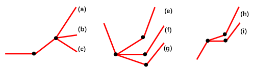
In the current deep learning research, the dominating network architectures are often not feedforward but intensively use shortcuts. However, the existing depth separation theory is established for feedforward networks. Few studies, if not none, considered the depth separation theory in the shortcut paradigm. Due to the pervasiveness of shortcuts, examining the depth separation in the context of shortcuts is critical. Here we are motivated by ResNet, which are outer links embedded into a network horizontally (Figure 1(b)). The shallow network with residual connections can have comparable performance with a deep network, i.e., the insertion of residual connections can save depth. Per structural symmetry, we embed shortcuts vertically, i.e., intra-linking neurons within a layer (Figure 1(c)) to force a neuron to take the outputs of its neighboring neuron. From the perspective of the crossing number Telgarsky (2016), the non-symmetric structure of intra-layer linked networks can produce more oscillations than networks without intra-layer links. Thus, intra-layer links can save width, i.e., without the need to go as wide as before, a shallow network can express as a complicated function as a deep network could, which means that the depth separation theory is modified.
Specifically, our roadmap to the modification of depth separation theorems includes two milestones. 1) Through bound analysis, explicit construction, and functional space analysis, we substantiate that a network with intra-layer links can produce much more pieces than a feedforward network, and the gain is at most exponential, i.e., , where is the number of hidden layers. 2) Since intra-layer links can yield more pieces, they can modify depth separation theorems by empowering a shallow network to represent a function constructed by a deep network, even if the width of this shallow network is lower than the prescribed threshold. The modification is done in the cases of vs 3 (Theorem 4.18), vs (Theorem 4.19, the famous sawtooth function (Telgarsky, 2015)), and Theorem 4.17. The saving of width is up to linear.
Although the focus of our draft is the depth separation theory, our result is also valuable in the following two aspects: First, the identified mechanism of generating more pieces can be translated into other shortcut networks such as ResNet and DenseNet, e.g., residual connections can represent a sawtooth function efficiently. Second, exploring new and powerful network architectures has been the mainstream research direction in deep learning in the past decade. To the best of our knowledge, we are the first to consider adding shortcuts within a layer in a fully-connected network. Our analysis theoretically suggests that an intra-linked network is more powerful than a feedforward network. Like the residual connections, we spotlight that the improvement of representation power by intra-layer links favorably increases no trainable parameters for a network.
To summarize, our contributions are threefold. 1) We point out the limitation of the depth separation theory and propose to consider inserting intra-layer links in shallow networks. 2) We show via bound estimation, explicit construction, and functional space analysis that intra-layer links can make a ReLU network produce more pieces. 3) We modify the depth separation result including the famous Telgarsky (2015)’s theorem by demonstrating that a shallow network with intra-layer links does not need to go as wide as before to represent a function constructed by a deep network.
2 Related works
A plethora of depth separation studies have shown the superiority of deep networks over shallow ones from perspectives of complexity analysis and constructive analysis.
The complexity analysis is to characterize the complexity of the function represented by a neural network, thereby demonstrating that increasing depth can greatly maximize such a complexity measure. Currently, one of the most popular complexity measures is the number of linear regions because it conforms to the functional structure of the widely-used ReLU networks. For example, Pascanu et al. (2013); Montufar et al. (2014); Montúfar (2017); Serra et al. (2018); Hu and Zhang (2018); Hanin and Rolnick (2019) estimated the bound of the number of linear regions generated by a fully-connected ReLU network by applying Zaslavsky’s Theorem (Zaslavsky, 1997). Xiong et al. (2020) offered the first upper and lower bounds of the number of linear regions for convolutional networks. Other complexity measures include classification capabilities (Malach and Shalev-Shwartz, 2019), Betti numbers (Bianchini and Scarselli, 2014), trajectory lengths (Raghu et al., 2017), global curvature (Poole et al., 2016), and topological entropy (Bu et al., 2020). Please note that using complexity measures to justify the power of depth demands a tight bound estimation. Otherwise, it is insufficient to say that shallow networks cannot be as powerful as deep networks, since deep networks cannot reach the upper bound.
The construction analysis is to find a family of functions that are hard to approximate by a shallow network, but can be efficiently approximated by a deep network. Eldan and Shamir (2016) built a special radial function that is expressible by a 3-layer neural network with a polynomial number of neurons, but a 2-layer network can do the same level approximation only with an exponential number of neurons. Later, Safran and Shamir (2017) extended this result to a ball function, which is a more natural separation result. Venturi et al. (2021) generalized the construction of this type to a non-radial function. Telgarsky (2015, 2016) used an -layer network to construct a sawtooth function. Given that such a function has an exponential number of pieces, it cannot be expressed by an -layer network, unless the width is . Arora et al. (2016) estimated the maximal number of pieces a network can produce, and established the size-piece relation to advance the depth separation results from (, ) to (, ), where . Other smart constructions include polynomials (Rolnick and Tegmark, 2017), functions of a compositional structure (Poggio et al., 2017), Gaussian mixture models (Jalali et al., 2019), and so on. Our work also includes the construction, and we use an intra-linked network to efficiently build a sawtooth function.
3 Notation and Definition
Notation 1 (Feedforward networks). For an ReLU DNN with widths of hidden layers, we use to denote the input of the network. Let be the vector composed of outputs of all neurons in the -th layer. The pre-activation of the -th neuron in the -th layer and the corresponding neuron are given by
respectively, where is the ReLU activation and are parameters. The output of this network is for some , .
Notation 2 (Intra-linked networks) For an ReLU DNN with widths of hidden layers, we now assume that every neurons are intra-linked in the -th layer, where can divide without remainder. Similar to the classical ReLU DNN, we use and to denote the input and the vectorized outputs of the -th layer. The -th pre-activation in the -th layer and the output of the network are computed in the same way as classical feedforward networks. In an intra-linked network, the -th, , -th neurons in the -th layer are linked, and the -th, , -th neurons in the -th layer are linked. We prescribe
for . Especially, we are interested in the case every 2 neurons are linked in each layer (i.e., ) and the case all neurons in a layer are linked (i.e., ) in this work.
Notation 3 (sawtooth functions and breakpoints) we say a piecewise linear (PWL) function is of "-sawtooth" shape, if for . We say is a breakpoint of a PWL function , if the left hand and right hand derivative of at are not equal, i.e., .
Please note that stacking a layer is essentially different from inserting intra-layer links in terms of the fundamental mechanism of generating new pieces, the number of affine transforms being used, and the functional class.
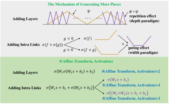
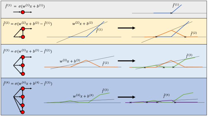
As Figure 2 shows, their mechanisms of producing pieces are fundamentally different. While the mechanism of adding a new layer is the repetition effect (multiplication), i.e., the function value of the function being composed is oscillating, and each oscillation can generate more pieces, which falls into the depth paradigm. The mechanism of intra-layer links is the gating effect (addition). The neuron being embedded have two activation states, and each state is leveraged to produce a breakpoint. Two states are integrated to generate more pieces. Such a mechanism essentially conforms to the parallelism, which is of width paradigm.
Adding intra-layer links does not increase the number of affine transforms and activations. As Figure 2 illustrates, a feedforward network with two layers involves two times of affine transformation (activation). In contrast, adding intra-layer links in a fully-connected layer actually exerts a gating effect. When , the output is ; when , the output is . The number of (affine transform, activation) is still one for both cases.
The function classes represented by our intra-linked network and the deeper feedforward network are not the same, either, and this will make a big difference. Given the same width, the deeper feedforward network has a larger function class than a shallow intra-linked network. However, given the same width and depth, our intra-linked network has more expressive power (i.e., number of pieces, VC dimension) than a feedforward network.
Since inserting intra-layer links is different from stacking new layers, we define the width and depth of intra-linked networks to be the same as the width and depth of feedforward networks resulting from removing intra-layer links.
Definition 3.1 (Width and depth of feedforward networks (Arora et al., 2016)).
For any number of hidden layers , input and output dimensions , an feedforward network is given by specifying a sequence of natural numbers representing widths of the hidden layers. The depth of the network is defined as , which is the number of (affine transform, activation). The width of the network is .
Definition 3.2 (Width and depth of intra-linked networks (Fan et al., 2020)).
Given an intra-linked network , we delete the intra-layer links to make the resultant network a feedforward network. Then, we define the width and depth of to be the same as the width and depth of .
4 Rethink the Depth Separation with Intra-layer Links
Since our focus is the network using ReLU activation and related estimation of the number of pieces, the seminal depth separation theorems closest to us are the following:
Theorem 4.1 (Depth separation vs (Telgarsky, 2015, 2016)).
For a natural number , there exists a sawtooth function representable by an -layer feedforward ReLU DNN of width such that if it is also representable by a -layer feedforward ReLU DNN, this -layer feedforward ReLU DNN should at least have the width of .
Theorem 4.2 (Depth separation vs (Arora et al., 2016)).
For every pair of natural numbers , there exists a function representable by an -layer feedforward ReLU DNN of width such that if it is also representable by a -layer feedforward ReLU DNN for any , this -layer feedforward ReLU DNN has width at least .
Despite being one-dimensional, the above results convincingly reveal that increasing depth can make a ReLU network express a much more complicated function, which is the heart of depth separation. Here, we shed new light on the depth separation problem with intra-layer links. Our primary argument is that if intra-layer links shown in Figure 1(c) are inserted, there exist shallow networks that previously cannot express some hard functions constructed by deep networks now can do the job. Our investigation consists of two parts. First, we substantiate that adding intra-layer links can greatly increase the number of pieces via bound estimation, explicit construction, and functional space analysis. Then, adding intra-layer links can represent complicated functions such as sawtooth functions, without the need of going as wide as before.
4.1 Intra-Layer Links Can Increase the Number of Pieces
4.1.1 Upper Bound Estimation
Lemma 4.3.
Let be a PWL function with pieces, then the breakpoints of consist of two parts: some old breakpoints of and at most newly produced breakpoints. Furthermore, has new breakpoints if and only if has distinct zero points.
Proof.
A direct calculus. ∎
Theorem 4.4 (Upper bound of feedforward networks).
Let be a PWL function represented by an ReLU DNN with depth and widths of hidden layers. Then has at most pieces.
This bound is the univariate case of the bound: , derived in Montúfar (2017) for -dimensional inputs. In Appendix B, we offer constructions to show that this bound is achievable in a depth-bounded but width-unbounded network (depth=3) (Proposition B.1) and a width-bounded (width=3) but depth-unbounded network (Proposition B.2) in one-dimensional space. Previously many bounds Pascanu et al. (2013); Montufar et al. (2014); Montúfar (2017); Xiong et al. (2020) on linear regions were derived, however, it is unknown whether these bounds are vacuous or tight, particularly for networks with more than one hidden layer. What makes Propositions B.1 and B.2 special is that they for the first time substantiate that Montúfar (2017)’s bound is tight over three-layer and deeper networks, although these results are for the one-dimensional case.
Remark 1. (Sharpening the bound in (Arora et al., 2016)). Previously, Arora et al. (2016) computed the number of pieces produced by a network of depth and widths as . The reason why their bound has an exponential term is that when considering how ReLU activation increases the number of pieces, they repetitively computed the old breakpoints generated in the previous layer. Our Lemma 4.3 implies that the ReLU activation in fact cannot double the number of pieces of a PWL function. Therefore, the depth separation theorem of Arora et al. (2016) needs to be re-examined.
Lemma 4.5.
Let be two PWL functions with totally breakpoints. Set and . Then the breakpoints of consist of three parts: some breakpoints of , some breakpoints of , and at most newly produced breakpoints. Furthermore, has newly produced breakpoints if and only if has distinct zero points.
Proof.
A direct corollary of Lemma 4.3. ∎
Let us illustrate why the intra-linked architecture can produce more pieces. Given two PWL functions and which has totally breakpoints, in the feedforward architecture, and have totally at most breakpoints, which contains at most old breakpoints of and at most newly produced breakpoints. However, in the intra-linked architecture, can produce more breakpoints because has two states: activated or deactivated. Then, and consist of at most old breakpoints of and newly produced breakpoints.
Theorem 4.6 (Upper bound of 2-neuron intra-linked networks).
Let be a PWL function represented by a ReLU DNN with depth , widths , and every two neurons linked in each hidden layer as Figure 1(c). Assuming that are even, has at most pieces.
Proof.
We prove by induction on . For the base case , we assume for every odd , the neurons and are linked. The number of breakpoints of , , is at most . Hence, the first layer yields at most pieces. For the induction step, we assume that for some , any ReLU DNN with every two neurons linked in each hidden layer, depth and widths of hidden layers produces at most pieces. Now we consider any ReLU DNN with every two neurons linked in each hidden layer, depth and widths of hidden layers. By the induction hypothesis, each has at most breakpoints. Then the breakpoints of consist of some breakpoints of and at most newly generated breakpoints. Then has at most breakpoints, based on Lemma 4.5. The breakpoints of consist of some breakpoints of and at most newly generated breakpoints. Note that have totally at most breakpoints. In all, the number of pieces we can therefore get is at most ∎
In the following theorems, we offer the bound estimation for high-dimensional cases. The detailed proof for Theorem 4.8 is put into Appendix A.
Theorem 4.7 (Upper Bound of Feedforward Networks (Montúfar, 2017)).
Let be a PWL function represented by an ReLU DNN with depth and widths of hidden layers. Then has at most linear regions.
Theorem 4.8 (Upper Bound of Intra-linked Networks).
Let be a PWL function represented by an ReLU DNN with every two neurons linked in each hidden layer, depth and widths of hidden layers. We assume each is even. Then has at most linear regions.
4.1.2 Explicit Construction.
Despite that the bound estimation offers some light, to convincingly illustrate that intra-layer links can increase the number of pieces, we need to supply the explicit construction for the intra-linked networks. The number of pieces in the construction should be bigger than either the upper bound of feedforward networks or the maximal number a feedforward network can achieve. Specifically, the constructions for 2-neuron intra-linked networks in Propositions 4.9 and 4.10 have a number of pieces larger than the upper bounds of feedforward networks. In Proposition 4.11, by enumerating all possible cases, we present a construction for a 2-neuron intra-linked network of width 2 and arbitrary depth whose number of pieces is larger than what a feedforward network of width 2 and arbitrary depth possibly achieves. Proposition 4.12 shows that pieces can be achieved by a one-hidden-layer all-intra-linked network. Propositions 4.13 and 4.14 provide rather tight constructions for an all-neuron intra-linked network of width 3&4 and arbitrary depth.
Proposition 4.9 (The bound is tight for a two-hidden-layer 2-neuron intra-linked network).
Given an two-hidden-layer ReLU network, with every two neurons linked in each hidden layer, for any even , there exists a PWL function represented by such a network, whose number of pieces is .
Proposition 4.10 (Use intra-linked networks to achieve a sawtooth function with pieces).
There exists a function represented by an intra-linked ReLU DNN with depth and width of hidden layers, whose number of pieces is at least .
Proposition 4.11 (Intra-layer links can greatly increase the number of pieces in an ReLU network with width 2 and arbitrary depth).
Let be a PWL function represented by an -layer ReLU DNN with widths of all hidden layers. Then the number of pieces of is at most
There exists an -layer -wide ReLU DNN, with neurons linked in each hidden layer, which can produce at least pieces.
Proof.
The proof is put in Appendix E. ∎
Proposition 4.12 ( pieces for a one-hidden-layer all-neuron intra-linked network).
Given an one-hidden-layer ReLU network with all neurons linked in the hidden layer, there exists a PWL function represented by such a network, whose number of pieces is .
Proof.
For the first layer, has one breakpoint and each has at most newly produced breakpoints and some old breakpoints of and , for . Hence, the first layer gives at most pieces. Then the rest of the proof is similar to Theorem 4.6. ∎
Proposition 4.13 (An arbitrarily deep network of width=3 and with all neurons in each layer intra-linked can achieve at least pieces).
There exists an function represented by an intra-linked ReLU DNN with depth , width in each layer, and all neurons intra-linked in each layer, whose number of pieces is at least .
Proposition 4.14 (An arbitrarily deep network of width=4 and with all neurons in each layer intra-linked can achieve at least pieces).
There exists an function represented by an intra-linked ReLU DNN with depth , width in each layer, and all neurons in each layer intra-linked, whose number of pieces is at least .
4.1.3 Functional Space Analysis
The above constructive analyses demonstrate that in the maximal sense, intra-layer links can empower a feedforward network to represent a function with more pieces. Now, we move one step forward by showing that intra-layer links can surprisingly expand the functional space of a feedforward network. The reason why this result is surprising is that one tends to think an intra-linked network produces an exclusively different function from a feedforward network. However, here we report that given an arbitrary feedforward ReLU network, adding intra-layer links in the first layer can definitely expand its functional space (Theorem 4.15). The core is that an intra-linked one-hidden-layer network of two neurons can express a feedforward one-hidden-layer network of two neurons, and the opposite doesn’t hold true.
Theorem 4.15.
Let be any PWL representable by a classical -layer ReLU DNN with widths of hidden layers. Then, can also be represented by a -layer ReLU DNN with widths of hidden layers, with neurons in the first layer linked.
Remark 2. Finding new and powerful network architectures has been always important in deep learning. Although the focus of our draft is the depth separation theory rather than designing new architectures, our analysis theoretically suggests that an intra-linked network is more powerful than a feedforward network. Moreover, since adding intra-layer links increases no trainable parameters, they can serve as an economical add-on to the model to use parameters more efficiently. Even if only every two neurons are intra-linked in a layer, the improvement is exponentially dependent on depth, i.e., approximately , which is considerable when a network is deep.
4.2 Modify the Depth Separation Theorem with Intra-layer Links
In a broad sense, the depth separation theorem consists of two elements: i) there exists a function representable by a deep network; ii) such a function cannot be represented by a shallow network whose width is lower than a threshold. Since adding intra-layer links can generally improve the capability of a network, if one adds intra-layer links to a shallow network, the function constructed by a deep network can be represented by a shallow network, even if the width of this shallow network is still lower than the threshold. Theorem 4.17 showcases that a shallow network with all-neuron intra-layer links can save the width up to a linear reduction. Theorems 4.18 and 4.19 modify the depth separation vs 3 and vs , respectively, by presenting that a shallow network with 2-neuron intra-layer links only needs to go times as wide as before to express the same function.
Lemma 4.16 (A network with width=2 can approximate any univariate PWL function (Fan et al., 2021)).
Given a univariate PWL function with pieces , there exists a -layer network with two neurons in each layer such that .
Theorem 4.17 (Modify the depth separation vs 2).
For every , there exists a function that can be represented by a -layer ReLU DNN with 2 nodes in each layer, such that it cannot be represented by a classical -layer ReLU DNN with width less than , but can be represented by a -layer, -wide intra-linked ReLU DNN .
Theorem 4.18 (Modify the depth separation vs 3).
For every , there exists a function that can be represented by a -layer ReLU DNN with 2 nodes in each layer, such that it cannot be represented by a classical -layer ReLU DNN with width less than , but can be represented by a -layer, -wide intra-linked ReLU DNN .
Theorem 4.19 (Modify the depth separation vs ).
For every , there is a PWL function represented by a feedforward -layer ReLU DNN with at most nodes in each layer, such that it cannot be represented by a classical -layer ReLU DNN with width less than , but can be represented by a -layer 2-neuron intra-linked ReLU DNN with width no more than .
Proof.
Per (Telgarsky, 2016)’s construction, a feedforward -layer ReLU DNN with at most nodes in each layer can produce a sawtooth function of pieces. Similarly, a feedforward -layer ReLU DNN with at most nodes in each layer can have pieces. Thus, it follows Theorem 4.4 that any classical -layer ReLU DNN with width less than cannot generate pieces. However, according to the construction in Proposition 4.10, let , an intra-linked network can exactly express a sawtooth function with pieces. ∎
Remark 3. The existing depth separation theory is established for feedforward networks. Our systematic analyses reveal that when considering shortcuts, the existing depth separation can be modified in terms of reducing the bar of width. Theorem 4.17 implicates that intra-layer links can reduce the bar of the width substantially (), where is the original width, with a linear reduction. Our highlight is the existence of such shallow networks that can be transformed by intra-layer links to have representation power on a par with a deep network. Such shallow networks go against the predictions of depth separation theory.
5 Discussion and Conclusion
Well-established network architectures such as ResNet and DenseNet imply that incorporating shortcuts greatly empowers a neural network. However, only a limited number of theoretical studies attempted to explain the representation ability of shortcuts Veit et al. (2016); Fan et al. (2021); Lin and Jegelka (2018). Although intra-layer links and residual connections are essentially two different kinds of shortcuts, the techniques we developed and the mechanisms we identified in analyzing intra-linked networks can be extended to other networks with shortcuts. On the one hand, we identified conditions for the tightness of the bound, which has been proven to be stronger than existing results. Specifically, in the activation step, we distinguish the existing and newly generated breakpoints to avoid repeated counting, and then in the following pre-activation step, we maximize the oscillation to yield the most pieces after the next activation. On the other hand, the construction of functions in our work, i.e., constructing oscillations by preserving existing breakpoints and splitting each piece into several ones, is generic in analyzing other popular types of networks, thereby explaining how the shortcut connections improve the representation power of a network.
For example, it is straightforward to see that a one-neuron-wide ReLU DNN can represent PWL functions with at most three pieces, no matter how deep the network is. However, as Theorem 5.1 shows, with residual connections, a ResNet with neurons can represent a sawtooth function with pieces, which cannot be done by a feedforward network. For DenseNet, Theorem 4.4 shows that an ReLU DNN with depth and width has at most pieces. If we add dense intra-layer links that connect any two neurons in a hidden layer to turn a feedforward network into a DenseNet, Theorem 5.2 shows that the so-obtained DenseNet can produce much more pieces than the feedforward network. The difference is exponential, i.e., vs . The detailed proofs are put into Appendix H.
Theorem 5.1.
Let be a PWL function represented by a one-neuron-wide ResNet. Mathematically, , where are parameters, for . Then has at most pieces. Furthermore, this upper bound is tight and can be a sawtooth function with at most pieces.
Theorem 5.2.
Let be a PWL function represented by a DenseNet obtained by adding dense intra=layer links into a feedforward network with depth and width of hidden layers. Then we can construct such a PWL function with at least pieces.
In this draft, via bound estimation, dedicated construction, and functional space analysis, we have shown that an intra-linked network is much more expressive than a feedforward one. Then, we have modified the depth separation results to that a shallow network that previously cannot express some functions constructed by deep networks now can do the job with intra-layer links. Our results supplement the existing depth separation theory, and suggest the potential of intra-layer links. At the same time, the identified mechanism of generating pieces can also be used to decode the power of other shortcut networks such as ResNet and DenseNet. Future endeavors can be training networks using intra-layer links to solve real-world problems.
References
- Arora et al. (2016) Raman Arora, Amitabh Basu, Poorya Mianjy, and Anirbit Mukherjee. Understanding deep neural networks with rectified linear units. arXiv preprint arXiv:1611.01491, 2016.
- Bianchini and Scarselli (2014) Monica Bianchini and Franco Scarselli. On the complexity of neural network classifiers: A comparison between shallow and deep architectures. IEEE transactions on neural networks and learning systems, 25(8):1553–1565, 2014.
- Bu et al. (2020) Kaifeng Bu, Yaobo Zhang, and Qingxian Luo. Depth-width trade-offs for neural networks via topological entropy. arXiv preprint arXiv:2010.07587, 2020.
- Eldan and Shamir (2016) Ronen Eldan and Ohad Shamir. The power of depth for feedforward neural networks. In Conference on learning theory, pages 907–940. PMLR, 2016.
- Fan et al. (2020) Feng-Lei Fan, Rongjie Lai, and Ge Wang. Quasi-equivalence of width and depth of neural networks. arXiv preprint arXiv:2002.02515, 2020.
- Fan et al. (2021) Fenglei Fan, Dayang Wang, Hengtao Guo, Qikui Zhu, Pingkun Yan, Ge Wang, and Hengyong Yu. On a sparse shortcut topology of artificial neural networks. IEEE Transactions on Artificial Intelligence, 2021.
- Gühring et al. (2020) Ingo Gühring, Mones Raslan, and Gitta Kutyniok. Expressivity of deep neural networks. arXiv preprint arXiv:2007.04759, 2020.
- Hanin and Rolnick (2019) Boris Hanin and David Rolnick. Deep relu networks have surprisingly few activation patterns. In Advances in Neural Information Processing Systems, pages 359–368, 2019.
- Hu and Zhang (2018) Qiang Hu and Hao Zhang. Nearly-tight bounds on linear regions of piecewise linear neural networks. arXiv preprint arXiv:1810.13192, 2018.
- Jalali et al. (2019) Shirin Jalali, Carl Nuzman, and Iraj Saniee. Efficient deep learning of gmms. arXiv preprint arXiv:1902.05707, 2019.
- Joshi et al. (2023) Chaitanya K Joshi, Cristian Bodnar, Simon V Mathis, Taco Cohen, and Pietro Liò. On the expressive power of geometric graph neural networks. arXiv preprint arXiv:2301.09308, 2023.
- LeCun et al. (2015) Yann LeCun, Yoshua Bengio, and Geoffrey Hinton. Deep learning. nature, 521(7553):436–444, 2015.
- Lin and Jegelka (2018) Hongzhou Lin and Stefanie Jegelka. Resnet with one-neuron hidden layers is a universal approximator. Advances in Neural Information Processing Systems, 31:6169–6178, 2018.
- Malach and Shalev-Shwartz (2019) Eran Malach and Shai Shalev-Shwartz. Is deeper better only when shallow is good? Advances in Neural Information Processing Systems, 32, 2019.
- Montúfar (2017) Guido Montúfar. Notes on the number of linear regions of deep neural networks. Sampling Theory Appl., Tallinn, Estonia, Tech. Rep, 2017.
- Montufar et al. (2014) Guido F Montufar, Razvan Pascanu, Kyunghyun Cho, and Yoshua Bengio. On the number of linear regions of deep neural networks. In Advances in neural information processing systems, pages 2924–2932, 2014.
- Pascanu et al. (2013) Razvan Pascanu, Guido Montufar, and Yoshua Bengio. On the number of response regions of deep feed forward networks with piece-wise linear activations. arXiv preprint arXiv:1312.6098, 2013.
- Poggio et al. (2017) Tomaso Poggio, Hrushikesh Mhaskar, Lorenzo Rosasco, Brando Miranda, and Qianli Liao. Why and when can deep-but not shallow-networks avoid the curse of dimensionality: a review. International Journal of Automation and Computing, 14(5):503–519, 2017.
- Poggio et al. (2020) Tomaso Poggio, Andrzej Banburski, and Qianli Liao. Theoretical issues in deep networks. Proceedings of the National Academy of Sciences, 117(48):30039–30045, 2020.
- Poole et al. (2016) Ben Poole, Subhaneil Lahiri, Maithra Raghu, Jascha Sohl-Dickstein, and Surya Ganguli. Exponential expressivity in deep neural networks through transient chaos. Advances in neural information processing systems, 29, 2016.
- Raghu et al. (2017) Maithra Raghu, Ben Poole, Jon Kleinberg, Surya Ganguli, and Jascha Sohl-Dickstein. On the expressive power of deep neural networks. In international conference on machine learning, pages 2847–2854. PMLR, 2017.
- Rolnick and Tegmark (2017) David Rolnick and Max Tegmark. The power of deeper networks for expressing natural functions. arXiv preprint arXiv:1705.05502, 2017.
- Safran and Lee (2022) Itay Safran and Jason Lee. Optimization-based separations for neural networks. In Conference on Learning Theory, pages 3–64. PMLR, 2022.
- Safran and Shamir (2017) Itay Safran and Ohad Shamir. Depth-width tradeoffs in approximating natural functions with neural networks. In International conference on machine learning, pages 2979–2987. PMLR, 2017.
- Safran et al. (2019) Itay Safran, Ronen Eldan, and Ohad Shamir. Depth separations in neural networks: what is actually being separated? In Conference on Learning Theory, pages 2664–2666. PMLR, 2019.
- Sanford and Chatziafratis (2022) Clayton H Sanford and Vaggos Chatziafratis. Expressivity of neural networks via chaotic itineraries beyond sharkovsky’s theorem. In International Conference on Artificial Intelligence and Statistics, pages 9505–9549. PMLR, 2022.
- Serra et al. (2018) Thiago Serra, Christian Tjandraatmadja, and Srikumar Ramalingam. Bounding and counting linear regions of deep neural networks. In International Conference on Machine Learning, pages 4558–4566. PMLR, 2018.
- Stanley (2004) Richard P. Stanley. An introduction to hyperplane arrangements. In Lecture Notes, IAS/Park City Mathematics Institute, 2004.
- Telgarsky (2015) Matus Telgarsky. Representation benefits of deep feedforward networks. arXiv preprint arXiv:1509.08101, 2015.
- Telgarsky (2016) Matus Telgarsky. Benefits of depth in neural networks. In Conference on learning theory, pages 1517–1539. PMLR, 2016.
- Vardi and Shamir (2020) Gal Vardi and Ohad Shamir. Neural networks with small weights and depth-separation barriers. Advances in neural information processing systems, 33:19433–19442, 2020.
- Vardi et al. (2021) Gal Vardi, Daniel Reichman, Toniann Pitassi, and Ohad Shamir. Size and depth separation in approximating benign functions with neural networks. In Conference on Learning Theory, pages 4195–4223. PMLR, 2021.
- Veit et al. (2016) Andreas Veit, Michael J Wilber, and Serge Belongie. Residual networks behave like ensembles of relatively shallow networks. Advances in neural information processing systems, 29, 2016.
- Venturi et al. (2021) Luca Venturi, Samy Jelassi, Tristan Ozuch, and Joan Bruna. Depth separation beyond radial functions. Journal of Machine Learning Research, 2021.
- Venturi et al. (2022) Luca Venturi, Samy Jelassi, Tristan Ozuch, and Joan Bruna. Depth separation beyond radial functions. The Journal of Machine Learning Research, 23(1):5309–5364, 2022.
- Xiong et al. (2020) Huan Xiong, Lei Huang, Mengyang Yu, Li Liu, Fan Zhu, and Ling Shao. On the number of linear regions of convolutional neural networks. In International Conference on Machine Learning, pages 10514–10523. PMLR, 2020.
- Zaslavsky (1975) T. Zaslavsky. Facing up to arrangements : face-count formulas for partitions of space by hyperplanes. Number 154 in Memoirs of the American Mathematical Society. American Mathematical Society, 1975.
- Zaslavsky (1997) T Zaslavsky. Facing up to arrangements: face-count formulas for partitions of space by hyperplanes. Memoirs of American Mathematical Society, 154:1–95, 1997.
Contents of Appendices
Section G extends the results of 2-intra-linked networks to a network with more intra-layer links.
Section H demonstrates that the analysis tools developed for intra-linked networks can also be used to analyze the power of ResNet and DenseNet.
Appendix A Proof of Theorem 4.8
Lemma A.1 (Zaslavsky’s Theorem Zaslavsky [1975], Stanley [2004]).
Let be an arrangement in . Then, the number of regions for the arrangement satisfies
| (1) |
Proof.
We prove by induction on . For the base case , produces one hyperplane in the input space . Furthermore, produces at most two hyperplanes in the input space . Therefore, in total, the neurons in the first layer produces hyperplanes in the input space . Then by Zaslavsky’s Theorem, it will produce at most linear regions in the input space . For the induction step, we assume that for some , any ReLU DNN with every two neurons linked in each hidden layer, depth and widths of hidden layers produces at most linear regions. Now we consider any ReLU DNN with every two neurons linked in each hidden layer, depth and widths of hidden layers. Then for each linear region produced by the first layers, again, produces one hyperplane in . Furthermore, produces at most two hyperplanes in the . Therefore, in total, the neurons in the layer produces hyperplanes in . Then by Zaslavsky’s Theorem, it will produce at most linear regions in . Thus has at most linear regions. ∎
Appendix B Supplementary Results for the Tightness of Theorem 4.4
Proposition B.1 (The bound is tight for a depth-bounded but width-unbounded network).
Given an two-hidden-layer ReLU network, for any width in the first and second hidden layers, there exists a PWL function represented by such a network, whose number of pieces is .
Proof.
To guarantee the bound is tight, the following two requirements should be met: (i) each , , , has distinct zero points that are as much as its number of pieces, so that the activation step can produce the most new breakpoints; (ii) the breakpoints of each , , , as the affine combination of , contains all the breakpoints of , so that all the old breakpoints are reserved.
Now we give the proof in detail. Let . When , we set
When , we let and
Then has distinct zero points. Hence for , the breakpoints of keeps all breakpoints of and yields new breakpoints. Note that and do not share new breakpoints, and and covers all the breakpoints of . Therefore, the total number of pieces via an affine combination of is pieces. ∎
Proposition B.2 (The bound is tight for a width-bounded but depth-unbounded network).
Given an ReLU network with width for the first layer and 3 for the other layers, for any depth , there exists a PWL function represented by such a network, whose number of pieces is .
Proof.
Let be the same as in Proposition B.1. Let
We set
Now we continue our proof by induction. Assume we have constructed , and , . Then we set
and
Through a direct calculus, we know has pieces with opposite slope in every two adjoint pieces and ranges from to in each piece except the leftmost and rightmost piece, which implied we can totally obtain pieces. ∎
Appendix C Proof of Proposition 4.9
Proposition C.1 (The bound is tight for a two-hidden-layer 2-neuron intra-linked network).
Given an two-hidden-layer ReLU network, with every two neurons linked in each hidden layer, for any even , there exists a PWL function represented by such a network, whose number of pieces is .
Proof.
To guarantee the bound is tight, the following two conditions should be satisfied: (i) and have as many zero points as possible so that and can produce the maximal number of breakpoints; (ii) all old breakpoints of are reserved by , an affine transform of .
We first consider the first hidden layer. Let
When , we set
When , for each odd , let where , then the output of the first layer is expressed as the following: which has pieces and whose adjacent pieces have slopes of opposite signs. Note that any line , where , can cross all pieces of . Thus, fulfills the conditions of Lemma 4.5. We divide the breakpoints of into two parts: and . We refer to their counts as # and #.
Next, we construct the second hidden layer. , where , has new breakpoints. Then by choosing some scaling parameter bias to fulfill Lemma 4.5, we can also make has distinct zero-points, which implies has newly produced breakpoints. Therefore, the affine combination of and contains all breakpoints of , and has # breakpoints. To reserve all the breakpoints of , we do the similar thing for to gain and , whose affine combination has # breakpoints, which contains all breakpoints in , and shares no breakpoints with the affine combination of .
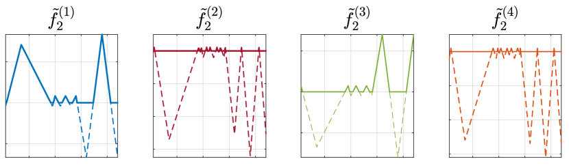
Hence, the affine combination of has # # breaking points, which contains all the breakpoints of . are visualized in Figure 4. Repeating this procedure by selecting different , we can construct the remaining such that the affine transformation of has pieces of . ∎
Appendix D Proof of Proposition 4.10
Proposition D.1 (Use intra-linked networks to achieve a sawtooth function with pieces).
There exists a function represented by an intra-linked ReLU DNN with depth and width of hidden layers, whose number of pieces is at least .
Proof.
Let defined over . The core of the proof is to use a one-hidden-layer network of neurons to create pieces from .
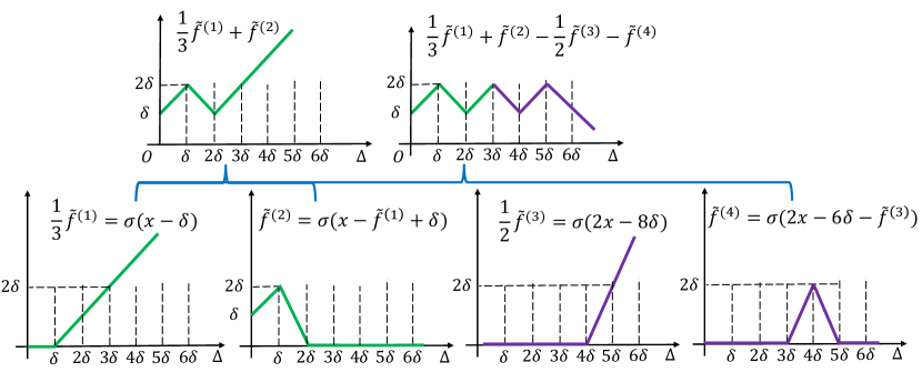
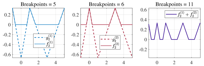
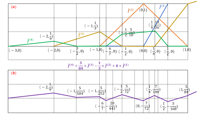
Let . Set , , , , and , , , , for all . The output of this one-hidden-layer network is which has pieces on . is of slope on , , and ranges from to on each piece. Figure 5 shows how the affine transformation of constructs a sawtooth function of 6 pieces. Please note that flipping or translating will not prevent from generating pieces.
The targeted intra-linked ReLU network with depth and width of hidden layers is designed as , where . ∎
Appendix E Proof of Proposition 4.11
Proof.
For the first assertion, we claim that each pre-activation , , , cannot have its every two adjacent pieces of slope with different sign, which implies the activation cannot produce the most breakpoints as in Lemma 4.3. In fact, , , has at most pieces. If some has pieces, then by exhaustion, we know either it has a -slope, or it has two adjacent pieces with slopes of the same sign (see Figure 6). Hence, , , has at most newly produced breakpoints. Then the output of the -nd layer has at most breakpoints, i.e., pieces. Applying a similar method to each piece, we can get our result via a simple induction step.
Now we come to the second assertion. For convenience, we say an PWL function is of "triangle-trapezoid-triangle" shape on , if there exists a partition of and a positive constant , such that
Given a PWL function of "triangle-trapezoid-triangle" shape on , with corresponding partition and , if we set
then is of "triangle-trapezoid-triangle" shape on respectively.
Using this fact, we can construct a PWL function represented by a -layer -wide intra-linked ReLU DNN, which has pieces. Actually, set
then through a direct calculus, is of "triangle-trapezoid-triangle" shape on . Using the fact above repeatedly, we can construct a PWL function represented by a -layer, -wide, intra-linked ReLU DNN, which is constant on and of "triangle-trapezoid-triangle" shape on , .
∎
Appendix F Proof of Theorem 4.15
Lemma F.1.
Let , where , and , there exists some , and such that , where .
Proof.
Without loss of generality, we assume and . Then is of slope , , and on and , respectively. Now we choose satisfying , and set . , . Then is of slope and on and , respectively, while is of slope 0, , and on , and , respectively. Hence, let , and , we have . ∎
Theorem F.2.
Let be any PWL representable by a classical -layer ReLU DNN with widths of hidden layers. Then, can also be represented by a -layer ReLU DNN with widths of hidden layers, with neurons in the first layer linked.
Proof.
Let the output of the -th neuron of the first layer in the feedforward network be , . Since the feedforward network is invariant to permutating neurons, we can link the arbitrary -th and -th neuron if , which directly concludes the proof according to Lemma F.1. ∎
Remark D.1. Generally, Theorem 4.15 does not hold for deeper layers. Since the first layer has only one input while the higher layer generally has several inputs so that Lemma F.1 does not hold. But Theorem 4.15 still holds for higher layers of some special networks. For example, the function class in Telgarsky [2015] is given by the composition of several functions, which makes the corresponding network has one neuron in every other layer.
Appendix G Extension to more intra-layer links
G.1 Proof of Proposition 4.12
Proof.
Without loss of generality, a one-hidden-layer network with all neurons intra-linked is mathematically formulated as the following:
| (2) |
To prove that the bound is tight for a one-hidden-layer network, the key is to make each produce new breakpoints and have non-zero pieces that share a point with . We use mathematical induction to derive our construction. Figure 7 schematically illustrates our construction idea.
First, let and . Note that has non-zero piece that shares a point with , and has non-zero pieces that share a common point with .
Then, given , we suppose has non-zero pieces that share a point with . Since is continuous, we select its peaks by the following conditions: i) is not differentiable at ; ii) . Next, let be the lowest peak of . As long as the slope and the bias satisfy
| (3) |
crosses and only crosses pieces of . These pieces are exactly non-zero pieces that share a point with . Thus, plus the breakpoint , generates a total of new breakpoints. At the same time, has non-zero pieces that share a point with . Figure 7 illustrates the process of induction.
Finally, the total number of breakpoints is , which concludes our proof.
∎
G.2 Proof of Proposition 4.14
Proof.
The core of the proof is to use a one-hidden-layer all-neuron-intra-linked network of width to create a quasi-sawtooth function with as many pieces as possible. We construct four neurons as follows:
| (4) |
The profiles of are shown in Figure 8(a).
By combining with carefully calibrated coefficients, we have the following quasi-sawtooth function that has pieces are
| (5) |
As shown in Figure 8(b), we have marked all breakpoints of to validate its correctness.
Next, we just need to let each layer of the intra-linked network represent a stretched and down-pulled variant of , e.g., the -th layer , where is a sufficiently large number and to ensure that is within the function range of .
Finally, the constructed network is
| (6) |
∎
G.3 Proof of Proposition 4.13
Proof.
Following the same spirit in proof of Theorem 4.14, we construct three neurons as follows:
| (7) |
The target function that returns us pieces is
| (8) |
Next, we just need to let each layer of the intra-linked network represent a stretched and down-pulled variant of , e.g., the -th layer , where is a sufficiently large number and to ensure that is within the function range of .
Finally, the constructed network is
| (9) |
∎
Appendix H Analysis Extended to ResNet and DenseNet
H.1 Proof of Theorem 5.1
Proof.
H.2 Proof of Theorem 5.2
Proof.
For convenience, we only consider the case , the general case is just simply repeating this procedure. Let
be the neurons of the first hidden layer. Then we consider the affine combination. It is easy to find coefficient such that
A direct calculus gives , shown in Figure 9. Then follow the same idea in analyzing intra-linked networks, we know all the non-constant pieces of can generate in the next layer and the result follows after a simple induction step. ∎
Theorem 5.1 confirms that adding simple links can greatly improve the representation ability of a network. Actually, both ResNet and intra-layer linked networks do not increase the number of parameters, but they can represent more complicated functions than the feedforward of the same neurons used in each layer. Hence, the linked structure can improve the efficiency of parameters. Besides, we can see from the proof of Theorem 5.1 and 5.2 that the idea and construction in analyzing intra-linked networks can indeed be utilized to analyze other architecture of networks.