Discrete integrable systems associated with relativistic collisions

Abstract

We study vector quadrirational Yang–Baxter maps representing the momentum-energy transformation of two particles after elastic relativistic collisions. The collision maps admit Lax representations compatible with an $r$-matrix Poisson structure and correspond to integrable systems of quadrilateral lattice equations.

1 Introduction

The integrability of discrete systems (systems of ordinary or partial difference equations) is closely related to the concept of multidimensional consistency. This can be depicted as the three-dimensional (3D) consistency for equations on two-dimensional lattices [3, 9, 31], with fields assigned to the vertices of elementary quadrilaterals, and as the (set theoretical) Yang–Baxter equation [7, 10, 16, 40, 44, 46] for maps with fields assigned to the edges of the quadrilaterals. Both the 3D consistency and the Yang–Baxter property reflect the compatibility of the equations/maps when extended to the three-dimensional lattice, and they are related to typical integrability features such as zero-curvature representations, Bäcklund–Darboux transformation, invariant Poisson structures, recursion operators, symmetries and conserved quantities (see e.g. [4, 5, 20, 25, 28, 29, 34, 44]).

In this article we study particle collision problems in the framework of discrete integrable systems. In [22], it was shown that the velocity transformation of two head-on elastically colliding particles satisfies the Yang–Baxter equation with the two masses acting as the Yang–Baxter parameters. In the classical (non-relativistic) case the collision Yang–Baxter map is linear and is linked to a discrete wave equation (see the relevant discussion in section 2.1). In the relativistic case, the induced collision map is a non-rational parametric Yang–Baxter map which can be transformed, under a non-rational change of variables, to a rational one associated with well-known integrable lattice equations of KdV type. This surprising link between discrete integrable systems and particle collision problems motivates this work.

The aim of this paper is to investigate various integrability aspects of relativistic collision problems which extend the results of [22]. We will introduce and study integrable, in the sense of multidimensional consistency, birational maps and affine linear equations associated with elastic collisions. In the non-relativistic case the velocity transformation under the collision of two particles generates linear systems that satisfy all the desirable properties. However, in the relativistic case we show that the momentum-energy vectors, rather than velocities, form a more natural set of variables. The momentum-energy transformation of the colliding particles is a vector quadrirational Yang–Baxter map which corresponds to an affine linear system of 3D consistent quadrilateral equations. Moreover, a higher-dimensional generalisation associated with planar collisions is presented, which admits a Lax representation compatible with the Sklyanin bracket. Thus we derive invariant Poisson structures for transfer maps, which represent particular sequences of periodic colliding particles, on the two-dimensional lattice and Poisson commuting first integrals.

Section 2 includes a short introduction to the theory of 3D consistent equations and Yang–Baxter maps. As a first application, we present the linear systems associated with classical elastic collisions. In section 3, we study head-on relativistic collisions. We review the velocity transformation map and introduce the momentum-energy transformation Yang–Baxter map, its Lax representation and the corresponding 3D consistent lattice equations. Higher dimensional generalisations of these systems are presented in section 4, where we also study invariant Poisson structures, reductions and the Liouville integrability of the transfer maps. We conclude in section 5 with further comments and perspectives for future work.

2 Integrable lattice equations, Yang–Baxter maps and classical collisions

We consider an equation of the form $Q(f,f_{1},f_{2},f_{12};\alpha,\beta)=0$, where the four variables $f,f_{1},f_{2},f_{12}\in\mathbb{C}^{n}$ are assigned to the four vertices of a quadrilateral and the parameters $\alpha,\beta$ are assigned to its edges (Figure 1). We assume that this equation is affine linear, that is linear with respect to any one of the arguments $f,f_{1},f_{2}$ and $f_{12}$. Next, we consider fixed values $f,f_{1},f_{2},f_{3}$ at four vertices of a cube as in Figure 1 (black points). By employing the same equation at the corresponding vertices of the down, front and left faces of the cube we can determine uniquely the values $f_{12},f_{13}$ and $f_{23}$. Hence, we can determine the value $f_{123}$ in three different ways by the rest three faces of the cube. If all these three values coincide, i.e. $f_{123}$ is uniquely defined as a function of $f,f_{1},f_{2},f_{3}$, then the equation $Q(f,f_{1},f_{2},f_{12};\alpha,\beta)=0$ is called 3D consistent or consistent around the cube [3, 9, 31].

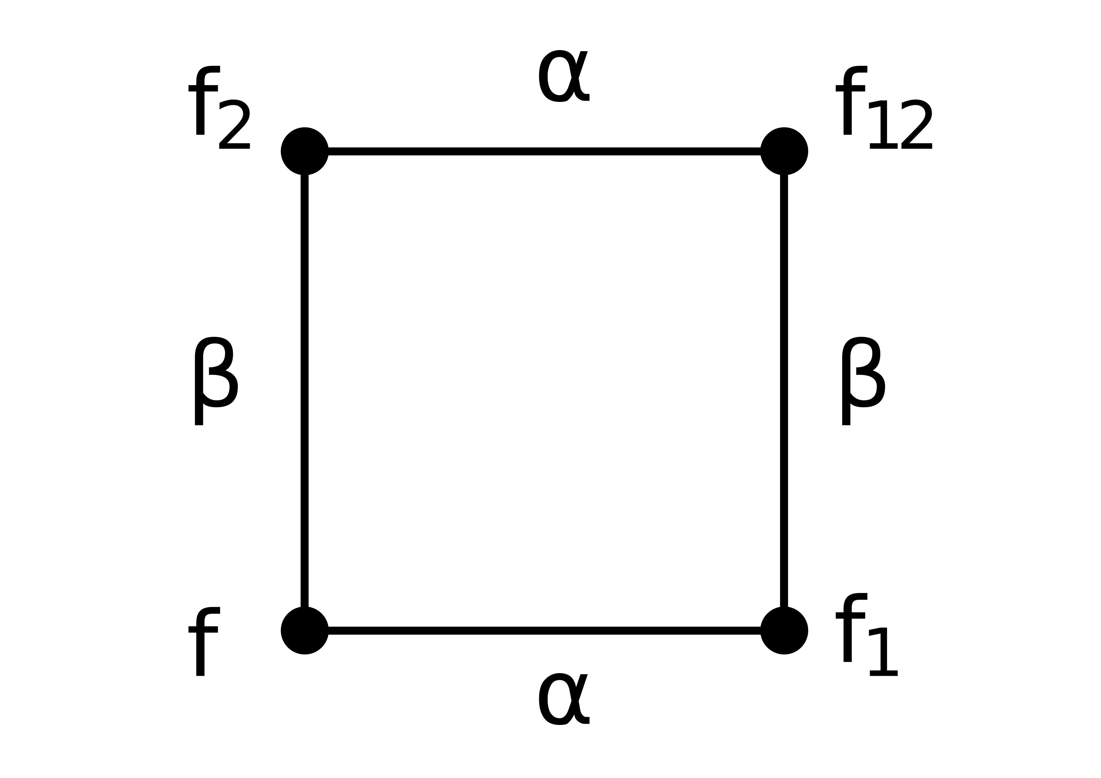
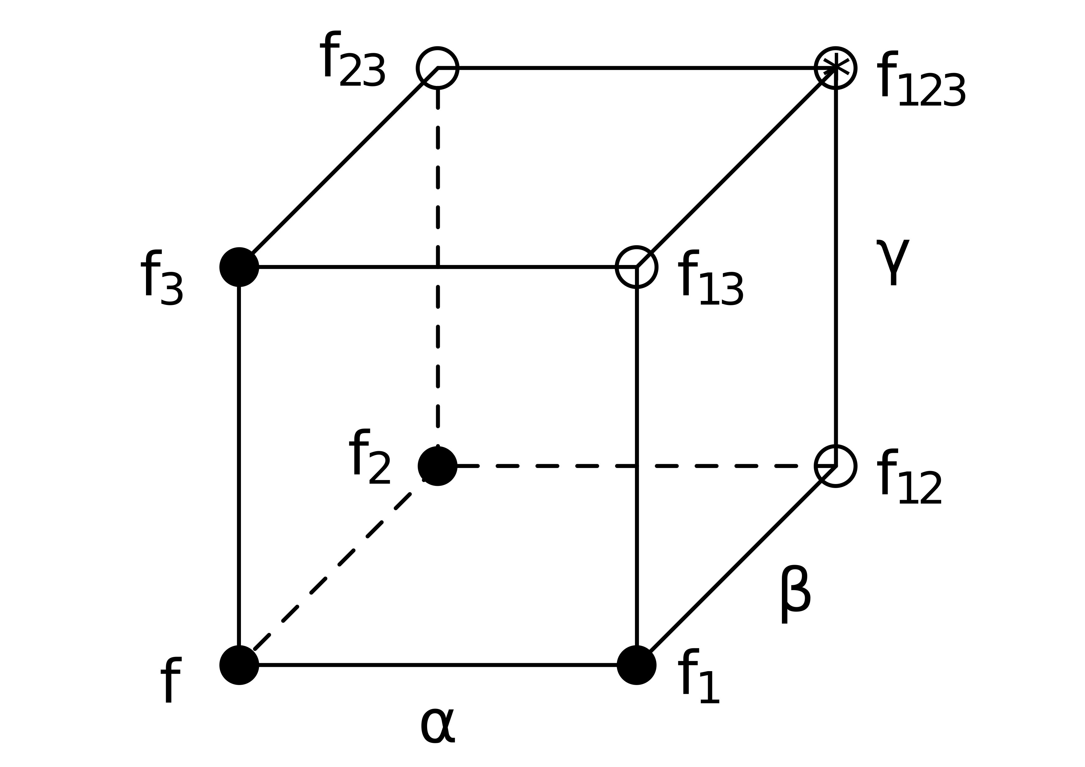
Figure 1: 3D consistency

We can regard the equation $Q(f,f_{1},f_{2},f_{12};\alpha,\beta)=0$ as defined on a two-dimensional quadrilateral lattice with fields $f_{i,j}:\mathbb{Z}^{2}\rightarrow\mathbb{C}^{n}$, by setting $f=f_{n,m},f_{1}=f_{n+1,m},f_{2}=f_{n,m+1}$ and $f_{12}=f_{n+1,m+1}$, thus

$$Q(f_{n,m},f_{n+1,m},f_{n,m+1},f_{n+1,m+1};\alpha,\beta)=0.$$ (1)

The 3D consistency then indicates that the lattice equation (1) can be embedded in a three dimensional lattice in a compatible way. Adler, Bobenko and Suris presented in [3] a classification of 3D consistent equations up to common Möbius transformations of the variables. An equivalent formulation of 3D consistency can be traced back in [5] (see also [26, 34]).

The equivalent of 3D consistency in the case of maps defined on the edges of a quadrilateral is the Yang–Baxter equation [7, 16, 46]. Following [10, 44], we will call a map $R:\mathcal{X}\times\mathcal{X}\rightarrow\mathcal{X}\times\mathcal{X}$, with $R:(x,y)\mapsto(u(x,y),v(x,y))$, a Yang–Baxter map if it satisfies the set-theoretical Yang–Baxter equation,

$$R_{23}\circ R_{13}\circ R_{12}=R_{12}\circ R_{13}\circ R_{23},$$ (2)

where $R_{ij}$, for $i,j=1,2,3$, denotes the action of the map $R$ on the $i$ and $j$ factor of $\mathcal{X}\times\mathcal{X}\times\mathcal{X}$, i.e. $R_{12}(x,y,z)=(u(x,y),v(x,y),z)$, $R_{13}(x,y,z)=(u(x,z),y,v(x,z))$ and $R_{23}(x,y,z)=(x,u(y,z),v(y,z))$. In general $\mathcal{X}$ can be any set, however here we will regard $\mathcal{X}$ as an algebraic variety. Furthermore, we will call the map $R$ quadrirational, if both maps $u(\cdot,y)$, $v(x,\cdot)$, for fixed $y$ and $x$ respectively, are birational isomorphisms of $\mathcal{X}$ to itself [4]. By considering $R$ as a map on the edges of an elementary quadrilateral, we can interpret the Yang–Baxter equation (2) as the compatibility of the map embedded on the faces of a 3D cube as in Figure 2.

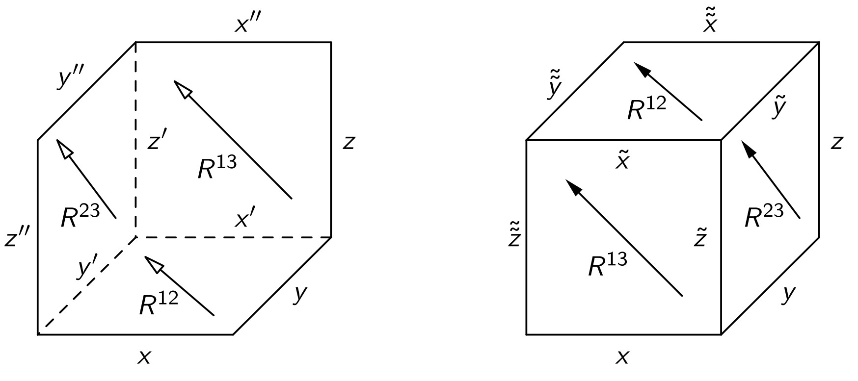
Figure 2: The cubic representation of the Yang–Baxter equation

A parametric Yang–Baxter map [44, 45] is a Yang–Baxter map $R:(\mathcal{X}\times\mathcal{I})\times(\mathcal{X}\times\mathcal{I})\mapsto(\mathcal{X}\times\mathcal{I})\times(\mathcal{X}\times\mathcal{I})$, with

$$R:((x,\alpha),(y,\beta))\mapsto((u,\alpha),(v,\beta))=((u(x,\alpha,y,\beta),\alpha),(v(x,\alpha,y,\beta),\beta)).$$ (3)

So, the Yang–Baxter parameters $\alpha,\beta\in\mathcal{I}$ are considered as extra variables that remain invariant under the map $R$. We usually keep the parameters $\alpha,\beta\in\mathcal{I}$ separate and denote (3) just by $R_{\alpha,\beta}:\mathcal{X}\times\mathcal{X}\rightarrow\mathcal{X}\times\mathcal{X}$. Classifications of parametric Yang–Baxter maps on $\mathbb{CP}^{1}\times\mathbb{CP}^{1}$ have been presented in [4, 35].

A matrix $L$ that depends on a point $x\in\mathcal{X}$, a parameter $\alpha\in\mathcal{I}$ and a spectral parameter $\zeta\in\mathbb{C}$, such that

$$L(u,\alpha,\zeta)L(v,\beta,\zeta)=L(y,\beta,\zeta)L(x,\alpha,\zeta)$$ (4)

is called a Lax matrix of the Yang–Baxter map $R_{\alpha,\beta}$ [43, 44, 45]. On the other hand, if $u=u_{\alpha,\beta}(x,y)$ and $v=v_{\alpha,\beta}(x,y)$ satisfy (4) for a matrix $L$ and the equation

$$L(\hat{x},\alpha,\zeta)L(\hat{y},\beta,\zeta)L(\hat{z},\gamma,\zeta)=L(x,\alpha,\zeta)L(y,\beta,\zeta)L(z,\gamma,\zeta)$$

implies the unique solution $\hat{x}=x,\ \hat{y}=y$ and $\hat{z}=z$ for every $x,y,z\in\mathcal{X}$, then it follows that the map $R_{\alpha,\beta}:(x,y)\mapsto(u,v)$ is a Yang–Baxter map with Lax matrix $L$ [23, 44].

3D consistent equations generate solutions of the Yang–Baxter equation and vice versa. This connection relies on the symmetries of the equations and the invariant conditions of the maps [18, 26, 33, 34, 37]. A similar approach can be considered for multi-component systems of difference equations [19]. The following proposition for Yang–Baxter maps defined on quasigroups which satisfy an invariant condition appears in [37] (see also [26] for applications in the case of parametric Yang–Baxter maps).

Proposition 2.1.

Let $R:L\times L\rightarrow L\times L$, $R(x,y)=(u(x,u),v(x,y))$ be a Yang–Baxter map on the quasigroup $(L,*)$ with $v(x,y)*u(x,y)=x*y$. Then

$$f_{n,m+1}=f_{n,m}*v(f_{n,m}\backslash f_{n+1,m},f_{n+1,m}\backslash f_{n+1,m+1})\;,$$ (5)

where $\backslash$ denotes the left division operation, is a 3D consistent equation.

In the case of an abelian group $(L,+)$, the invariant condition becomes $u(x,y)+v(x,y)=x+y$ and the corresponding 3D consistent equation

$$f_{n,m+1}=f_{n,m}+v(f_{n+1,m}-f_{n,m},f_{n+1,m+1}-f_{n+1,m})\;.$$ (6)

2.1 Classical head-on collision systems

As a first example, we consider the map $R^{0}_{m_{1},m_{2}}:(v_{1},v_{2})\mapsto(v_{1}^{\prime},v_{2}^{\prime})$, with

$$v_{1}^{\prime}=\frac{v_{1}(m_{1}-m_{2})+2m_{2}v_{2}}{m_{1}+m_{2}},\ v_{2}^{\prime}=\frac{v_{2}(m_{2}-m_{1})+2m_{1}v_{1}}{m_{1}+m_{2}}\;.$$ (7)

This linear map represents the transformation of velocities of two particles with masses $m_{1}$, $m_{2}$ respectively after elastic (non-relativistic) collision. Here $v_{1}$, $v_{2}$ denote the initial velocities of the two particles and $v_{1}^{\prime}$, $v_{2}^{\prime}$ the corresponding velocities after the collision.

The linear map $R^{0}_{m_{1},m_{2}}$ satisfies the parametric Yang–Baxter equation [22] and the invariant condition

$$m_{1}v_{1}+m_{2}v_{2}=m_{1}v_{1}^{\prime}+m_{2}v_{2}^{\prime}\;,$$

which reflects the conservation of momentum. The Yang–Baxter map $R^{0}_{m_{1},m_{2}}$ appears in various different contexts in literature. In [14], it describes the change of polarization throughout the tropical limit graph of soliton solutions of the vector KdV equation, while in [18] appears as a limit of Hirota’s KdV equation.

Now, if we consider vertex variables $w_{k,l}$ with

$$v_{1}=m_{2}(w_{k+1,l}-w_{k,l})\;,\ v_{1}=m_{1}(w_{k+1,l+1}-w_{k+1,l})\;,$$

$$v_{1}^{\prime}=m_{2}(w_{k+1,l+1}-w_{k,l+1})\;,\ v_{2}^{\prime}=m_{1}(w_{k,l+1}-w_{k,l})\;,$$

then equations (7) imply the discrete linear wave equation:

$$(m_{2}-m_{1})(w_{n+1,m+1}-w_{n,m})+(m_{2}+m_{1})(w_{n+1,m}-w_{n,m+1})=0\;.$$ (8)

We can show directly that (8) is a 3D consistent equation. Linear quadrilateral 3D consistent equations are described in [6] and linear Yang–Baxter maps in [11].

3 Head-on relativistic collisions and integrable lattice systems

In this section we present the Yang–Baxter maps and the integrable lattice equations associated with head-on relativistic collisions. The parametric Yang–Baxter map which corresponds to the velocity transformation is not a rational map but it is equivalent, under a non-rational change of variables which preserves the Yang–Baxter property, to a quadrirational one associated with the discrete modified and the Schwarzian KdV equations. On the other hand, the map that represents the momentum-energy transformation after collision is by default quadrirational. This (non-parametric) higher-dimensional map satisfies the Yang–Baxter equation too, and corresponds to a system of 3D consistent lattice equations.

3.1 Discrete systems associated with velocity transformations

In [22], we have shown that the transformation of the velocities of two head-on colliding particles with invariant masses $m_{1}$, $m_{2}$, after an elastic relativistic collision is given by the collision map

$$\mathcal{R}_{m_{1},m_{2}}=(\phi^{-1}\times\phi^{-1})\circ{R}_{m_{1},m_{2}}\circ(\phi\times\phi),$$ (9)

where $\phi:(-c,c)\rightarrow(0,+\infty)$ is the bijection $\phi(v)=\sqrt{\frac{c+v}{c-v}}$, $(\phi\times\phi)(v_{1},v_{2})=(\phi(v_{1}),\phi(v_{2}))$, $c$ is the speed of light and $R_{m_{1},m_{2}}$ the quadrirational map

$${R}_{m_{1},m_{2}}(x,y)=\left(y\left(\frac{m_{1}x+m_{2}y}{m_{2}x+m_{1}y}\right),x\left(\frac{m_{1}x+m_{2}y}{m_{2}x+m_{1}y}\right)\right):=(u,v)\;.$$ (10)

Both maps, $R_{m_{1},m_{2}}$ and $\mathcal{R}_{m_{1},m_{2}}$ are parametric Yang–Baxter maps with Lax matrices

$$L(x,\alpha,\zeta)=\left(\begin{array}[]{cc}\zeta&\alpha x\\ \frac{\alpha}{x}&\zeta\end{array}\right)\ \text{and}\ \mathcal{L}(x,m_{1},\zeta)=L(\phi(x),m_{1},\zeta)$$ (11)

respectively.

The collision map (9) is not rational but it is equivalent under the non-rational transformation $\phi$ to the quadrirational Yang–Baxter map (10) (for the Yang–Baxter equivalence see [35]). The latter map corresponds to the $H_{III}^{A}$ map of the classification list in [35] under the transformation $x\mapsto\alpha\hat{x}$, $y\mapsto\beta\hat{y}$, $u\mapsto\alpha\hat{u}$, $v\mapsto\beta\hat{v}$ and the reparametrization $\alpha^{2}=\hat{\alpha},\ \beta^{2}=\hat{\beta}$, and to the $F_{III}$ map of the classification list in [4], for $x\mapsto-\alpha x$, $y\mapsto\beta\hat{y}$, $u\mapsto\alpha\hat{u}$, $v\mapsto-\beta\hat{v}$ and the same reparametrization.

Now, from (10), by setting $x=w_{k+1,l}w_{k,l}$, $y=w_{k+1,l+1}w_{k+1,l}$, $u=w_{k+1,l+1}w_{k,l+1}$ and $v=w_{k,l+1}w_{k,l}$, we come up with the 3D consistent equation

$$w_{k+1,l}(\alpha w_{k,l}+\beta w_{k+1,l+1})-w_{k,l+1}(\beta w_{k,l}+\alpha w_{k+1,l+1})=0\;,$$ (12)

which is a discrete version of the potential modified KdV equation [30] and corresponds under a gauge transformation to $H_{3}$ equation in [3] (for $\delta=0$). We can derive this equation directly from Proposition 2.1 by considering the quasigroup $L=\mathbb{C}\backslash\{0\}$ with binary operation $x*y=\frac{y}{x}$, for any $x,y\in L$, (so that the left division is then defined as $x\backslash y=xy$), which also proves the 3D consistency of this equation.

There is one more 3D consistent equation associated with the Yang–Baxter map (10) and the invariant condition $m_{1}u+m_{2}v=m_{1}x+m_{2}y$, that is the discrete Schwarzian KdV or cross-ratio lattice equation ($Q_{1}$ for $\delta=0$ of the ABS classification list [3]),

$$\frac{(w_{k,l}-w_{k,l+1})(w_{k+1,l+1}-w_{k+1,l})}{(w_{k,l+1}-w_{k+1,l+1})(w_{k+1,l}-w_{k,l})}=\frac{m_{2}^{2}}{m_{1}^{2}}\;,$$ (13)

which is obtained by considering vertex variables $w_{k,l}$, such that $m_{2}(w_{k+1,l}-w_{k,l})=x$, $m_{1}(w_{k+1,l+1}-w_{k+1,l})=y$, $m_{2}(w_{k+1,l+1}-w_{k,l+1})=u$ and $m_{1}(w_{k,l+1}-w_{k,l})=v$.

3.2 Discrete systems associated with momentum-energy
transformations

We consider the two colliding particles with rest masses $m_{1}$, $m_{2}$ and initial momentum-energy vectors

$$\mathbf{x}=(x_{0},x_{1})=(\frac{E_{x}}{c},p_{x})\;,\ \mathbf{y}=(y_{0},y_{1})=(\frac{E_{y}}{c},p_{y})\;$$

respectively. Here, $E_{x},E_{y}$ denote the relativistic energy of the two particles before collision and $p_{x},p_{y}$ their momenta. We also denote by

$$\mathbf{u}=(u_{0},u_{1})=(\frac{E_{u}}{c},p_{u})\;,\ \mathbf{v}=(v_{0},v_{1})=(\frac{E_{v}}{c},p_{v})\;$$

the momentum-energy vectors of the particles after collision, with $E_{u},E_{v}$ and $p_{u},p_{v}$ their corresponding energies and momenta. The conservation of relativistic energy and momentum then reads

$$\mathbf{u}+\mathbf{v}=\mathbf{x}+\mathbf{y}\;.$$ (14)

Furthermore, the energy-momentum relation, $E^{2}=(pc^{2})+(mc^{2})^{2}$, for each particle implies that

$$u_{0}^{2}-u_{1}^{2}=x_{0}^{2}-x_{1}^{2}=m_{1}^{2}c^{2}\;,\ v_{0}^{2}-v_{1}^{2}=y_{0}^{2}-y_{1}^{2}=m_{2}^{2}c^{2}\;.$$ (15)

The system of (14) and (15) admits two solutions with respect to $\mathbf{u}$ and $\mathbf{v}$, the trivial one $\mathbf{u}=\mathbf{x}$, $\mathbf{v}=\mathbf{y}$, which corresponds to no-collision, and the collision solution

$$\mathbf{u}=\mathbf{y}+k(\mathbf{x},\mathbf{y})(\mathbf{x}+\mathbf{y})\;,\mathbf{v}=\mathbf{x}-k(\mathbf{x},\mathbf{y})(\mathbf{x}+\mathbf{y})\;,$$ (16)

with

$$k(\mathbf{x},\mathbf{y})=\frac{({x}_{0}^{2}-{x}_{1}^{2})-({y}_{0}^{2}-{y}_{1}^{2})}{(x_{0}+y_{0})^{2}-(x_{1}+y_{1})^{2}}=\frac{\langle\mathbf{x},\mathbf{x}\rangle-\langle\mathbf{y},\mathbf{y}\rangle}{\langle\mathbf{x}+\mathbf{y},\mathbf{x}+\mathbf{y}\rangle}\;.$$ (17)

Here, by $\langle\ ,\ \rangle$ we denote the bilinear form $\langle\mathbf{x},\mathbf{y}\rangle:=x_{0}y_{0}-x_{1}y_{1}$. Hence, the invariant conditions (14)-(15) imply that $\langle\mathbf{x},\mathbf{x}\rangle=\langle\mathbf{u},\mathbf{u}\rangle$, $\langle\mathbf{y},\mathbf{y}\rangle=\langle\mathbf{v},\mathbf{v}\rangle$ and $k(\mathbf{x},\mathbf{y})=k(\mathbf{u},\mathbf{v})$.

Now, we define as the momentum-energy map the map

$$\mathbf{R}:(\mathbf{x},\mathbf{y})\mapsto(\mathbf{u},\mathbf{v}):=(\mathbf{y}+k(\mathbf{x},\mathbf{y})(\mathbf{x}+\mathbf{y}),\mathbf{x}-k(\mathbf{x},\mathbf{y})(\mathbf{x}+\mathbf{y}))\;,$$ (18)

which maps the initial collision momentum-energy vectors of the two particles to the corresponding vectors after collision.

Proposition 3.1.

The momentum-energy map (18) is a (non-parametric) quadrirational Yang–Baxter map with Lax matrix

$$\mathbf{L}(\mathbf{x},\zeta)=\left(\begin{array}[]{cc}\zeta&\ x_{0}+x_{1}\\ x_{0}-x_{1}&\zeta\end{array}\right).$$ (19)

Proof.

The Yang–Baxter property of the map $\mathbf{R}$ can be checked directly. We can also verify that for $\mathbf{u}=\mathbf{y}+K(\mathbf{x}+\mathbf{y})$ and $\mathbf{v}=\mathbf{x}-K(\mathbf{x}+\mathbf{y})$,

$$\mathbf{L}(\mathbf{u},\zeta)\mathbf{L}(\mathbf{v},\zeta)=\mathbf{L}(\mathbf{y},\zeta)\mathbf{L}(\mathbf{x},\zeta)\;,$$

which shows that $\mathbf{L}(\mathbf{x},\zeta)$ is a Lax matrix of $\mathbf{R}$. Finally, the quadrirationality of $\mathbf{R}$ follows by observing that system (16) is equivalent to

$$\mathbf{u}=-\mathbf{v}+k(\mathbf{x},-\mathbf{v})(\mathbf{x}-\mathbf{v})\;,\ \mathbf{y}=-\mathbf{x}+k(\mathbf{x},-\mathbf{v})(\mathbf{x}-\mathbf{v})\;,$$

and to

$$\mathbf{v}=-\mathbf{u}+k(\mathbf{u},-\mathbf{y})(\mathbf{u}-\mathbf{y})\;,\ \mathbf{x}=-\mathbf{y}+k(\mathbf{u},-\mathbf{y})(\mathbf{u}-\mathbf{y})\;.$$

∎

Remark 3.2.

If we replace the quadratic form $\langle\mathbf{x},\mathbf{y}\rangle=x_{0}y_{0}-x_{1}y_{1}$ that appears in the momentum-energy map (18) with the scalar product $\langle\mathbf{x},\mathbf{y}\rangle=x_{0}y_{0}+x_{1}y_{1}$ of the Euclidean space $\mathbb{R}^{2}$, then we retrieve a map $R_{k}$ which (up to a permutation) was presented in [1] as integrable deformations of a polygon. The two maps are not equivalent in the real space $\mathbb{R}^{2}\times\mathbb{R}^{2}$. The map $R_{k}$ preserves the circles $x_{0}^{2}+x_{1}^{2}=c_{1}^{2}$ and $y_{0}^{2}+y_{1}^{2}=c_{2}^{2}$, for constants $c_{1},c_{2}$, while the momentum-energy map $\mathbf{R}$ the parabolas $x_{0}^{2}-x_{1}^{2}=m_{1}^{2}c^{2}$ and $y_{0}^{2}-y_{1}^{2}=m_{2}^{2}c^{2}$. However, the two maps are equivalent by considering a complex change of variables. That is

$${R}_{k}=(\phi\times\phi)\circ{\mathbf{R}}\circ(\phi^{-1}\times\phi^{-1})\;,$$

for $\phi(x_{0},x_{1})=(x_{0},ix_{1})$.

The momentum-energy Yang–Baxter map (18) is reversible, which means that $\mathbf{R}_{21}\circ\mathbf{R}=Id$ and it is an involution, $\mathbf{R}\circ\mathbf{R}=Id$. Moreover, it is associated with a system of 3D consistent lattice equation. We can derive this equation from proposition 2.1 by considering the abelian group $(\mathbb{R}^{2},+)$ and the invariant condition (14). In this case, equation (6) becomes

$$\mathbf{w}_{n+1,m}-\mathbf{w}_{n,m+1}=k(\mathbf{w}_{n+1,m}-\mathbf{w}_{n,m},\mathbf{w}_{n+1,m+1}-\mathbf{w}_{n+1,m})(\mathbf{w}_{n+1,m+1}-\mathbf{w}_{n,m})\;.$$ (20)

We can derive this system directly from the map (18) by setting

$$\mathbf{x}=\mathbf{w}_{n+1,m}-\mathbf{w}_{n,m},\ \ \ \mathbf{y}=\mathbf{w}_{n+1,m+1}-\mathbf{w}_{n+1,m},$$

$$\mathbf{u}=\mathbf{w}_{n+1,m+1}-\mathbf{w}_{n,m+1},\ \mathbf{v}=\mathbf{w}_{n,m+1}-\mathbf{w}_{n,m}.$$

For the vertex variables $\mathbf{w}_{n,m}=(f_{n,m},g_{n,m})$, the system (20) is expressed as

$$\frac{(f_{n+1,m+1}-f_{n,m+1})^{2}-(f_{n+1,m}-f_{n,m})^{2}}{(g_{n+1,m+1}-g_{n,m+1})^{2}-(g_{n+1,m}-g_{n,m})^{2}} =1\;,$$ (21)

$$\frac{(f_{n+1,m+1}-f_{n+1,m})^{2}-(f_{n,m+1}-f_{n,m})^{2}}{(g_{n+1,m+1}-g_{n+1,m})^{2}-(g_{n,m+1}-g_{n,m})^{2}} =1\;.$$ (22)

The vector equation (20), or equivalently system (21)-(22), is uniquely solvable with respect to any one of the arguments $\mathbf{w}_{n,m}=(f_{n,m},g_{n,m})$, $\mathbf{w}_{n+1,m}=(f_{n+1,m},g_{n+1,m})$, $\mathbf{w}_{n,m+1}=(f_{n,m+1},g_{n,m+1})$ and $\mathbf{w}_{n+1,m+1}=(f_{n+1,m+1},g_{n+1,m+1})$. Its 3D consistency follows from proposition 2.1. We can also obtain a Lax representation for this system from the Lax representation (19) of the momentum-energy map, i.e. the solutions of (20) satisfy the equation

$$\mathbf{L}(\mathbf{w}_{n+1,m+1}-\mathbf{w}_{n,m+1},\zeta)\mathbf{L}(\mathbf{w}_{n,m+1}-\mathbf{w}_{n,m},\zeta)=\mathbf{L}(\mathbf{w}_{n+1,m+1}-\mathbf{w}_{n+1,m},\zeta)\mathbf{L}(\mathbf{w}_{n+1,m}-\mathbf{w}_{n,m},\zeta).$$

4 Higher dimensional generalisations

The aim of this section is to generalise the results of the head-on collisions in higher dimensions. We will mainly focus on the two-dimensional space case. So, we consider that the two colliding particles, with rest masses $m_{1}$ and $m_{2}$, have two-dimensional vector momentums $\mathbf{p}_{x}=(p_{x_{1}},p_{x_{2}})$, $\mathbf{p}_{y}=(p_{y_{1}},p_{y_{2}})$ and $\mathbf{p}_{u}=(p_{u_{1}},p_{u_{2}})$, $\mathbf{p}_{v}=(p_{v_{1}},p_{v_{2}})$ before and after collision respectively. We also denote by $E_{x}$, $E_{y}$, and $E_{u}$, $E_{v}$ the corresponding relativistic energies of the particles and we define the momentum-energy vectors

$$\mathbf{x}=(x_{0},x_{1},x_{2}):=(\frac{E_{x}}{c},\mathbf{p}_{x})\;,\ \mathbf{y}=(y_{0},y_{1},y_{2}):=(\frac{E_{y}}{c},\mathbf{p}_{y})\;,$$

$$\mathbf{u}=(u_{0},u_{1},u_{2}):=(\frac{E_{u}}{c},\mathbf{p}_{u})\;,\ \mathbf{v}=(v_{0},v_{1},v_{2}):=(\frac{E_{v}}{c},\mathbf{p}_{v})\;.$$

The conservation of relativistic energy and momentum along with the energy-momentum relation imply the system

$$\mathbf{u}+\mathbf{v}=\mathbf{x}+\mathbf{y}\;,\ \langle\mathbf{u},\mathbf{u}\rangle=\langle\mathbf{x},\mathbf{x}\rangle\;,\ \langle\mathbf{v},\mathbf{v}\rangle=\langle\mathbf{y},\mathbf{y}\rangle\;,$$ (23)

where $\langle\ ,\ \rangle$ denotes the quadratic form $\langle\mathbf{x},\mathbf{y}\rangle:=x_{0}y_{0}-x_{1}y_{1}-x_{2}y_{2}$.

The system (23) consists of five equations, so more information is needed to derive a unique solution with respect to $\mathbf{u}$ and $\mathbf{v}$. This could be, for instance, one of $u_{i}$, $v_{i}$, or the scattering angle of the two colliding particles after the collision, and can be linked to an extra parameter.

4.1 A 2D collision Yang–Baxter map

In this section, we present a higher dimensional Yang–Baxter map associated with relativistic collisions on the plane, which satisfies an extra parametric invariant condition. This map generalises the head-on collision Yang–Baxter maps of the previous section and corresponds to a system of 3D consistent lattice equations.

Theorem 4.1.

The map $\mathbf{\hat{R}}_{\alpha,\beta}:(\mathbf{x},\mathbf{y})\mapsto(\mathbf{u},\mathbf{v})$, with

$$\mathbf{u}=\ \hat{k}(\mathbf{x},\mathbf{y},q)\mathbf{x}+(1-\hat{k}(\mathbf{y},\mathbf{x},q))\mathbf{y}+2q\hat{\mathbf{r}}(\mathbf{x},\mathbf{y},q)\;,$$ (24)

$$\mathbf{v}=(1-\hat{k}(\mathbf{x},\mathbf{y},q))\mathbf{x}+\hat{k}(\mathbf{y},\mathbf{x},q)\mathbf{y}-2q\hat{\mathbf{r}}(\mathbf{x},\mathbf{y},q)\;,$$ (25)

where

$$\hat{k}(\mathbf{x},\mathbf{y},q)=\frac{\langle\mathbf{x},\mathbf{x}\rangle-\langle\mathbf{y},\mathbf{y}\rangle+q^{2}}{\langle\mathbf{x}+\mathbf{y},\mathbf{x}+\mathbf{y}\rangle+q^{2}}\;,\ \hat{\mathbf{r}}(\mathbf{x},\mathbf{y},q) =\frac{(x_{1}y_{2}-x_{2}y_{1},x_{0}y_{2}-x_{2}y_{0},x_{1}y_{0}-x_{0}y_{1})}{\langle\mathbf{x}+\mathbf{y},\mathbf{x}+\mathbf{y}\rangle+q^{2}}\;,$$

and $q=\alpha-\beta$, is a parametric quadrirational Yang–Baxter map which satisfies the invariant conditions (23) and admits a Lax representation with Lax matrix

$${\mathbf{L}(\mathbf{x},\alpha,\zeta)}=\left(\begin{array}[]{cc}\zeta+i(x_{2}-\alpha)&\ x_{0}+x_{1}\\ x_{0}-x_{1}&\zeta-i(x_{2}+a)\end{array}\right).$$ (26)

Proof.

For every generic $2\times 2$ matrices $X$, $Y$, $U$ and $V$, the system (factorization system)

$$(U-\zeta I)(V-\zeta I)=(Y-\zeta I)(X-\zeta I),$$

together with the equation $\det(U-\zeta I)=\det(X-\zeta I)$, where $I$ indicates the identity matrix, admits a non-trivial solution with respect to $U$ and $V$, that is

$$U=(YX-\det(X)I)(Y+X-\mathrm{Tr}(X)\,I)^{-1}\;,\ V=Y+X-U\;.$$

The map $\mathcal{R}_{I}:(X,Y)\mapsto(U,V)$ defined by this solution is a quadrirational Yang–Baxter map with Lax matrix $X-\zeta I$, and invariant conditions $\det(U)=\det(X)$, $\det(V)=\det(Y)$, $\mathrm{Tr}(U)=\mathrm{Tr}(X)$ and $\mathrm{Tr}(V)=\mathrm{Tr}(Y)$. This fact is proved in [23, 25].

Now, if we express the generic elements of the matrix $X$ as

$$[X]_{11}=i(x_{3}+x_{2}),\ [X]_{12}=x_{0}+x_{1},\ [X]_{21}=x_{0}-x_{1},\ [X]_{22}=i(x_{3}-x_{2})$$

and in a similar way the elements of the matrices $Y$, $U$ and $V$, then the map $\mathbf{\hat{R}}_{\alpha,\beta}$ constitutes the reduction of the map $\mathcal{R}_{I}$ to the invariant level sets

$$\{(x_{1},x_{2},x_{3},x_{4})\,|\,\mathrm{Tr}(X)=-2i\alpha\},\ \{(y_{1},y_{2},y_{3},y_{4})\,|\,\mathrm{Tr}(Y)=-2i\beta\},$$ (27)

by setting $x_{3}=u_{3}=-\alpha$ and $y_{3}=v_{3}=-\beta$. The same reduction at the Lax representation of $\mathcal{R}_{I}$ implies the Lax representation of $\mathbf{\hat{R}}_{\alpha,\beta}$ with Lax matrix (26). Hence, the Yang–Baxter property, the Lax representation, the quadrirationality and the invariant conditions of $\mathbf{\hat{R}}_{\alpha,\beta}$ follow from the corresponding properties of the Yang–Baxter map $\mathcal{R}_{I}$ under this reduction. ∎

The parametric map $\mathbf{\hat{R}}_{\alpha,\beta}$ of theorem 4.1 preserves the relativistic energy and momenta of the system of two colliding particles, as well as the rest masses $m_{1}$ and $m_{2}$. It is derived as the unique solution with respect to $\mathbf{u}$ and $\mathbf{v}$ of the factorization problem

$$\mathbf{L}(\mathbf{u},\alpha,\zeta)\mathbf{L}(\mathbf{v},\beta,\zeta)=\mathbf{L}(\mathbf{x},\alpha,\zeta)\mathbf{L}(\mathbf{y},\beta,\zeta).$$ (28)

In addition, from the Lax representation we can trace the extra parametric invariant condition

$$\alpha u_{0}+\beta v_{0}+(v_{1}u_{2}-u_{1}v_{2})=\alpha x_{0}+\beta y_{0}+(x_{1}y_{2}-y_{1}x_{2})\;,$$

or equivalently

$$\frac{\det(\mathbf{p}_{u},\mathbf{p}_{v})+\det(\mathbf{p}_{x},\mathbf{p}_{y})}{u_{0}-x_{0}}=q\;,$$ (29)

for $q=\alpha-\beta$. On the other hand, we can derive directly (24)-(25) from the unique solution of the system of (23) and (29), i.e. (28) is equivalent to (23),(29). Hence, $\mathbf{\hat{R}}_{\alpha,\beta}$ represents two-dimensional relativistic collisions which satisfy the parametric invariant condition (29).

The actual values of $\mathbf{\hat{R}}_{\alpha,\beta}$ depend only on the difference $q$ of the Yang–Baxter parameters $\alpha$ and $\beta$. The parameter $q$ can be related to the extra information which is required to fully determine planar collisions. For example, the scattering angle $\theta_{L}$ of the first particle with respect to the first axis is expressed with respect to the parameter $q$ and the initial conditions $\mathbf{x}$, $\mathbf{y}$ by the equation

$$\tan{\theta_{L}}=\frac{u_{2}}{u_{1}}=\frac{(|\mathbf{x}|^{2}-|\mathbf{y}|^{2}+q^{2})x_{2}+2(|\mathbf{x}|^{2}+\langle\mathbf{x},\mathbf{y}\rangle)y_{2}+2q(x_{1}y_{0}-x_{0}y_{1})}{(|\mathbf{x}|^{2}-|\mathbf{y}|^{2}+q^{2})x_{1}+2(|\mathbf{x}|^{2}+\langle\mathbf{x},\mathbf{y}\rangle)y_{1}+2q(x_{0}y_{2}-x_{2}y_{0})}\;,$$ (30)

where here $|\mathbf{x}|^{2}=\langle\mathbf{x},\mathbf{x}\rangle$ and $|\mathbf{y}|^{2}=\langle\mathbf{y},\mathbf{y}\rangle.$

We will further investigate the role of the parameters of the map $\mathbf{\hat{R}}_{\alpha,\beta}$ in a special case. So, we consider a frame (lab frame) in which the second particle is at rest and the velocity of the first particle is directed along the first axis, that is $y_{1}=y_{2}=x_{2}=0$ and $x_{1}>0$. In this case, taking into account the energy-momentum relation for the two particles, $|\mathbf{x}|^{2}=m_{1}^{2}c^{2}$ and $|\mathbf{y}|^{2}=m_{2}^{2}c^{2}$, (30) becomes

$$\tan{\theta_{L}}=\frac{2qy_{0}}{|\mathbf{x}|^{2}-|\mathbf{y}|^{2}+q^{2}}=\frac{2qm_{2}c}{m_{1}^{2}c^{2}-m_{2}^{2}c^{2}+q^{2}}\;.$$ (31)

In addition, we can express the scattering angle $\theta_{L}$ in the lab frame with respect to the scattering angle $\theta$ in the center-of-momentum frame, where the total momentum of the system is zero, by the formula

$$\tan{\theta_{L}}=\frac{m_{2}c^{2}\sin{\theta}}{E_{x}^{\prime}+E_{y}^{\prime}\cos{\theta}}=\frac{2c^{2}m_{2}\tan{\frac{\theta}{2}}}{E_{x}^{\prime}+E_{y}^{\prime}+(E_{x}^{\prime}-E_{y}^{\prime})\tan^{2}{\frac{\theta}{2}}}\;,$$ (32)

where here $E^{\prime}_{x}$ and $E^{\prime}_{y}$ denote the relativistic energies of the two particles before collision with respect to the center-of-momentum frame (so, $E_{x}^{\prime 2}-E_{y}^{\prime 2}=c^{4}(m_{1}^{2}-m_{2}^{2})$ ). Comparing (31) and (32), we derive that

$$q=\frac{1}{c}(E^{\prime}_{x}-E^{\prime}_{y})\tan{\frac{\theta}{2}}\;.$$ (33)

The particles’ after collision energies $E^{\prime}_{u}$ and $E^{\prime}_{v}$ with respect to the center of momentum frame are equal to $E^{\prime}_{x}$ and $E^{\prime}_{y}$ respectively. Thus, according to (33), a natural choice for the Yang–Baxter parameters $\alpha,\beta$ in this case is

$$\alpha=\frac{E^{\prime}_{x}}{c}\tan{\frac{\theta}{2}}=\frac{E^{\prime}_{u}}{c}\tan{\frac{\theta}{2}}\;,\ \beta=\frac{E^{\prime}_{y}}{c}\tan{\frac{\theta}{2}}=\frac{E^{\prime}_{v}}{c}\tan{\frac{\theta}{2}}\;.$$ (34)

Alternatively, if we denote by $W$ the invariant mass of the system of the particles defined by

$$W^{2}c^{2}=\langle\mathbf{x}+\mathbf{y},\mathbf{x}+\mathbf{y}\rangle=\langle\mathbf{u}+\mathbf{v},\mathbf{u}+\mathbf{v}\rangle=\frac{(E^{\prime}_{x}+E^{\prime}_{y})^{2}}{c^{2}}\;,$$

then from (33) we can express the parameter $q$ in terms of $\theta$, $W$, $m_{1}$ and $m_{2}$, as

$$q=\frac{c}{W}(m_{1}^{2}-m_{2}^{2})\tan{\frac{\theta}{2}}\;,$$

and consider

$$\alpha=\frac{cm_{1}^{2}}{W}\tan{\frac{\theta}{2}}\;,\ \beta=\frac{cm_{2}^{2}}{W}\tan{\frac{\theta}{2}}\;.$$

4.2 Poisson structure, reductions and transfer dynamics

The construction of the Lax matrix (26), as appears in the proof of theorem 4.1, suggests that it admits a compatible $r$-matrix Poisson structure, that is the Sklyanin bracket [38, 39]. Indeed, the equation

$$\{\mathbf{L}(\mathbf{x},{\alpha},i\zeta)\ \overset{\otimes}{,}\ \mathbf{L}(\mathbf{x},{\alpha},ih)\}=[\frac{{{P}}}{\zeta-\eta},\mathbf{L}(\mathbf{x},{\alpha},i\zeta)\otimes\mathbf{L}(\mathbf{x},{\alpha},ih)]\;,$$ (35)

where $P$ denotes the permutation operator, ${{P}}(x\otimes y)=y\otimes x$ and $\mathbf{L}$ the Lax matrix (26), is equivalent to

$$\{x_{0},x_{1}\}=x_{2}\;,\ \{x_{0},x_{2}\}=-x_{1}\;,\ \{x_{1},x_{2}\}=-x_{0}\;.$$ (36)

We can extend the Sklyanin bracket on $\mathcal{L}\times\mathcal{L}$, for $\mathcal{L}=\{\mathbf{L}(\mathbf{x},\alpha,\zeta)|\mathbf{x}\in\mathbb{R}^{3},\alpha\in\mathbb{R}\}$ by considering

$$\{\mathbf{L}(\mathbf{x},{\alpha},i\zeta)\ \overset{\otimes}{,}\ \mathbf{L}(\mathbf{x},{\alpha},ih)\}=[\frac{P}{\zeta-\eta},\mathbf{L}(\mathbf{x},{\alpha},i\zeta)\otimes\mathbf{L}(\mathbf{x},{\alpha},ih)]\;,$$

$$\{\mathbf{L}(\mathbf{y},{\beta},i\zeta)\ \overset{\otimes}{,}\ \mathbf{L}(\mathbf{y},{\beta},ih)\}=[\frac{P}{\zeta-\eta},\mathbf{L}(\mathbf{y},{\beta},i\zeta)\otimes\mathbf{L}(\mathbf{y},{\beta},ih)]\;,$$

and $\{\mathbf{L}(\mathbf{x},{\alpha},i\zeta)\ \overset{\otimes}{,}\ \mathbf{L}(\mathbf{y},{\beta},ih)\}=0$, which corresponds to the Poisson tensor

$$\pi_{(\mathbf{x},\mathbf{y})} ={x_{2}}\frac{\partial}{\partial x_{0}}\wedge\frac{\partial}{\partial x_{1}}-{x_{1}}\frac{\partial}{\partial x_{0}}\wedge\frac{\partial}{\partial x_{2}}-{x_{0}}\frac{\partial}{\partial x_{1}}\wedge\frac{\partial}{\partial x_{2}}$$

$$+{y_{2}}\frac{\partial}{\partial y_{0}}\wedge\frac{\partial}{\partial y_{1}}-{y_{1}}\frac{\partial}{\partial y_{0}}\wedge\frac{\partial}{\partial y_{2}}-{y_{0}}\frac{\partial}{\partial y_{1}}\wedge\frac{\partial}{\partial y_{2}}\;$$

on $\mathbb{R}^{3}\times\mathbb{R}^{3}$. Now, we can show directly that the Yang–Baxter map $\mathbf{\hat{R}}_{\alpha,\beta}$ of theorem 4.1 is Poisson with respect to $\pi_{(x,y)}$. This follows from the fact that $\mathbf{\hat{R}}_{\alpha,\beta}$ is a reduction on the Poisson submanifolds defined by the invariant level sets (27), of the more general Poisson Yang–Baxter map $\mathcal{R}_{I}$ (see proof of theorem 4.1) with respect to the Sklyanin bracket [23, 25].

The Poisson structure (36) is of rank two and it admits the Casimir function

$$\mathcal{C}({\mathbf{x}})=\langle\mathbf{x},\mathbf{x}\rangle=x_{0}^{2}-x_{1}^{2}-x_{2}^{2}\;.$$

Correspondingly, the extended (rank-four) Poisson structure $\pi_{(\mathbf{x},\mathbf{y})}$ admits the Casimirs $\mathcal{C}({\mathbf{x}})$ and $\mathcal{C}({\mathbf{y}})$. Since the Yang–Baxter map $\mathbf{\hat{R}}_{\alpha,\beta}$ preserves the Casimirs, we can further reduce it to a symplectic Yang–Baxter map (with the masses as extra Yang–Baxter parameters) on the four-dimensional invariant symplectic leaves of $\pi_{(\mathbf{x},\mathbf{y})}$ defined by the connected components of

$$\mathcal{S}_{m_{1},m_{2}}=\{(\mathbf{x},\mathbf{y})\,|\,\mathcal{C}({\mathbf{x}})=m_{1}^{2}c^{2},\ \mathcal{C}({\mathbf{y}})=m_{2}^{2}c^{2}\}\;.$$

However, the resulting map under this reduction is not rational.

The head-on collision Yang–Baxter map (18) is derived by reduction of $\mathbf{\hat{R}}_{\alpha,\beta}$ for $q=0$, i.e. $\alpha=\beta$, on an invariant manifold. Particularly, from (24)-(25) we observe that if we set $x_{2}=y_{2}=0$, for $q=0$, then we obtain $u_{2}=v_{2}=0$, which shows that

$$\mathcal{M}=\{(x_{0},x_{1},0,y_{0},y_{1},0):x_{i},y_{i}\in\mathbb{R}\}$$

is an invariant manifold of $\mathbf{\hat{R}}_{\alpha,\beta}$. The reduced map on $\mathcal{M}$ coincides with the head-on momentum-energy Yang–Baxter map (18).

The dynamical behaviour of a plain Yang–Baxter map is usually rather trivial. For example all the maps of the classification in [4, 35] are involutions and the same is true for the maps (9), (10) and (18) (but not for the higher-dimensional Yang–Baxter map of theorem 4.1). Nevertheless, for any Yang–Baxter map various families of multidimensional maps, usually referred as transfer maps, can be generated that exhibit highly non-trivial behaviour. In [44, 45], Veselov introduced an hierarchy of commuting transfer maps which preserve the spectrum of their monodromy matrix. The transfer maps of the collision Yang–Baxter maps represent particular sequences of $n$ colliding particles and their commutativity reflects the fact that the resulting momentum-energy vectors are independent of the ordering of the collisions.

Here, we will focus on a variant of Veselov’s transfer maps associated with periodic staircase initial value problems of integrable lattice equations [32, 36] (see also [24, 22] for the case of Yang–Baxter maps). In this framework, we define the transfer map of a Yang–Baxter map $R_{\alpha,\beta}$, as the map

$$T_{n}:(x_{1},x_{2},\dots,x_{n},y_{1},y_{2}\dots,y_{n})\mapsto(x_{1}^{\prime},x_{2}^{\prime}\dots,x_{n}^{\prime},y_{2}^{\prime},y_{3}^{\prime}\dots,y_{n}^{\prime},y_{1}^{\prime}),$$

where $(x_{i}^{\prime},y_{i}^{\prime})=R_{\alpha,\beta}(x_{i},y_{i})$, and the $k$-transfer map as the map $T_{n}^{k}:=\underbrace{T_{n}\circ\dots\circ T_{n}}_{k}$. We also define the monodromy matrix $M_{n}$ of $T_{n}$, with

$$M_{n}(x_{1},\dots,x_{n},y_{1},\dots,y_{n})=\prod_{i=0}^{n-1}L(y_{n-i},\beta,\zeta)L(x_{n-i},\alpha,\zeta)\;.$$

From the definition of the monodromy matrix and the Lax representation (4), it follows that

$$L(y_{1}^{\prime},\beta,\zeta)M_{n}(x_{1},\dots,x_{n},y_{1},\dots,y_{n})=M_{n}(T_{n}(x_{1},\dots,x_{n},y_{1},\dots,y_{n}))L(y_{1}^{\prime},\beta,\zeta)\;.$$ (37)

Hence, we can derive integrals of any transfer map from the spectrum of the monodromy matrix. Similarly, we can show that in the more general case of (non-autonomous) transfer maps including different parameters $\alpha_{i},\beta_{i}$, where $(x_{i}^{\prime},y_{j}^{\prime}):=R_{\alpha_{i},\beta_{j}}(x_{i},y_{j})$, the $n$-transfer map $T_{n}^{n}$ preserves the spectrum of the corresponding monodromy matrix.

Let us denote by $\mathbf{T}_{n}$ the $6n$-dimensional transfer map of the Yang–Baxter map $\mathbf{\hat{R}}_{\alpha,\beta}$, and by $\mathbf{M}(\zeta)=\mathbf{M}_{n}(\mathbf{x}_{1},\dots,\mathbf{x}_{n},\mathbf{y}_{1},\dots,\mathbf{y}_{n})$ and $\mathbf{M^{\prime}}(\zeta)=\mathbf{M}_{n}(\mathbf{T}_{n}(\mathbf{x}_{1},\dots,\mathbf{x}_{n},\mathbf{y}_{1},\dots,\mathbf{y}_{n}))$ the corresponding monodromy matrices. By construction, we obtain three linear integrals of $\mathbf{T}_{n}$ (associated with the invariant condition $\mathbf{u}+\mathbf{v}=\mathbf{x}+\mathbf{y}$ of $\mathbf{\hat{R}}_{\alpha,\beta}$),

$$I_{k}=\sum_{i=1}^{n}(x_{i}+y_{i})\;,\ k=0,1,2\;,$$

which represent the conservation of energy and momentum. More integrals are obtained from the spectrum of $\mathbf{M}(\zeta)$.

The comultiplication property of the Sklyanin bracket (see e.g. [41, 42] for the Sklyanin bracket with regard to the Heisenberg magnetic chain) implies that

$$\{\mathbf{M}(i\zeta)\ \overset{\otimes}{,}\ \mathbf{M}(ih)\}=[\frac{{{P}}}{\zeta-\eta},\mathbf{M}(i\zeta)\otimes\mathbf{M}(ih)]\;,$$

and from (37) we derive that $\{\mathbf{M}^{\prime}(i\zeta)\ \overset{\otimes}{,}\ \mathbf{M}^{\prime}(ih)\}=[\frac{{{P}}}{\zeta-\eta},\mathbf{M}^{\prime}(i\zeta)\otimes\mathbf{M}^{\prime}(ih)]\;,$ which shows that $\mathbf{T}_{n}$ is a Poisson map with respect to the (extended) Sklyanin bracket on $\mathbb{R}^{6n}$,

$$\pi_{(\mathbf{x}_{1},\mathbf{y}_{1})}+\pi_{(\mathbf{x}_{2},\mathbf{y}_{2})}+\dots+\pi_{(\mathbf{x}_{n},\mathbf{y}_{n})}\;.$$

Finally, the Sklyanin bracket ensures that the integrals obtained from the spectrum of $\mathbf{M}(\zeta)$ are in involution [8]. We summarise all these results in the following proposition.

Proposition 4.2.

The transfer map $\mathbf{T}_{n}$ is Poisson with respect to the Sklyanin bracket and preserves the spectrum of the monodromy matrix $\mathbf{M}(\zeta)$, the corresponding $2n$ Casimirs $\mathcal{C}({\mathbf{x}_{i}})$, $\mathcal{C}({\mathbf{y}_{i}})$ and the three linear integrals $I_{k}$. Furthermore, $\{tr\mathbf{M}(\zeta),tr\mathbf{M}(\eta)\}=0$.

Similar results hold also for Veselov’s transfer maps of $\mathbf{\hat{R}}_{\alpha,\beta}$. In order to complete a proof of the Liouville integrability of the transfer maps we need to show that the spectrum of the monodromy matrix generates enough functional independent integrals. In the future we aim to investigate in detail the Liouville integrability of several types of collision transfer maps.

4.3 The Lattice equation associated with 2D collisions

As in the case of head-on collisions, we can derive a $3$D-consistent system of lattice equations associated with the Yang–Baxter map $\mathbf{\hat{R}}_{\alpha,\beta}$ of theorem 4.1. Here, we apply proposition 2.1 on the abelian group $(\mathbb{R}^{3},+)$ by considering the invariant condition $\mathbf{u}+\mathbf{v}=\mathbf{x}+\mathbf{y}$, for $\mathbf{u}$ and $\mathbf{v}$ given by (24) and (25) respectively. In this case, equation (6) for the vector vertex variables $\mathbf{w}_{n,m}=(f_{n,m},g_{n,m},h_{n,m})$ implies the $3$D-consistent system

$$\mathbf{w}_{n+1,m}-\mathbf{w}_{n,m+1} =\hat{k}(\mathbf{w}_{n+1,m}-\mathbf{w}_{n,m},\mathbf{w}_{n+1,m+1}-\mathbf{w}_{n+1,m},q)(\mathbf{w}_{n+1,m}-\mathbf{w}_{n,m})$$

$$-\hat{k}(\mathbf{w}_{n+1,m+1}-\mathbf{w}_{n+1,m},\mathbf{w}_{n+1,m}-\mathbf{w}_{n,m},q)(\mathbf{w}_{n+1,m+1}-\mathbf{w}_{n+1,m})$$

$$+2q\hat{\mathbf{r}}(\mathbf{w}_{n+1,m}-\mathbf{w}_{n,m},\mathbf{w}_{n+1,m+1}-\mathbf{w}_{n+1,m},q)\;.$$ (38)

Similarly to the head-on collision system (20), we can derive system (4.3) directly from (24)-(25) by setting $\mathbf{x}=\mathbf{w}_{n+1,m}-\mathbf{w}_{n,m}$, $\mathbf{y}=\mathbf{w}_{n+1,m+1}-\mathbf{w}_{n+1,m}$, $\mathbf{u}=\mathbf{w}_{n+1,m+1}-\mathbf{w}_{n,m+1}$ and $\mathbf{v}=\mathbf{w}_{n,m+1}-\mathbf{w}_{n,m}$.

System (4.3) is uniquely solvable with respect to any one of the arguments $\mathbf{w}_{n,m}$, $\mathbf{w}_{n+1,m}$, $\mathbf{w}_{n,m+1}$, $\mathbf{w}_{n+1,m+1}$ and 3D consistent according to proposition 2.1. Furthermore, it admits the Lax representation

$$\mathbf{L}(\mathbf{w}_{n+1,m+1}-\mathbf{w}_{n,m+1},\alpha,\zeta)\mathbf{L}(\mathbf{w}_{n,m+1}-\mathbf{w}_{n,m},\beta,\zeta)$$

$$=\mathbf{L}(\mathbf{w}_{n+1,m+1}-\mathbf{w}_{n+1,m},\beta,\zeta)\mathbf{L}(\mathbf{w}_{n+1,m}-\mathbf{w}_{n,m},\alpha,\zeta)\;.$$

where $\mathbf{L}(\mathbf{w}_{n+1,m+1}-\mathbf{w}_{n,m+1},\alpha,\zeta)$ is the Lax matrix (26). The system (4.3) is reduced to (20) for $q=0$ and $h_{n,m}=0$, for all $n,m\in\mathbb{Z}$.

In some cases compatible Poisson structures of Yang–Baxter maps of particular form give rise to compatible Poisson structures for periodic reductions of the corresponding 3D-consistent lattice equations [27]. However, this connection is not completely clear yet and a straightforward implementation of the results in [27] do not apply here. We will defer this problem for a future work in which we intend to study invariant Poisson structures for the periodic reductions of relativistic collision quadrilateral equations.

5 Conclusion

In this paper, we presented discrete integrable systems, namely Yang–Baxter maps and 3D consistent systems of lattice equations, associated with elastic relativistic particle collisions. Our approach was based on the momentum-energy transformation which generalises the results of [22] and implies quadrirational Yang–Baxter maps, with respect to the original energy and momentum variables, as well as affine linear quadrilateral equations. Parametric generalisations of these systems, regarding planar relativistic collisions, were also presented, along with an $r$-matrix formalism suitable to study the Liouville integrability of the transfer maps. A complete proof of the Liouville integrability, including the investigation of exact solutions of transfer maps and of plane wave reductions of the induced lattice systems require further study.

The transfer maps of the Yang–Baxter maps and the periodic reductions of the quadrilateral equations correspond to periodic boundary conditions on two-dimensional lattices. Nevertheless, a similar approach to [12, 13] can be considered to study reflection maps and fixed boundary value problems for the discrete collision systems. Furthermore, various non-commutative and anti-commutative solutions of the Yang–Baxter equation appear in literature [2, 4, 15, 17, 21]. It would be interesting to examine the existence of non-commutative analogues of the collision Yang–Baxter maps and the corresponding 3D consistent equations.

Proceeding to higher-dimensional collision problems requires extra information regarding the colliding particles and equivalent parametric invariant conditions. The existence of higher-dimensional refactorization problems which reproduce such conditions, in addition to the conservation of momentum-energy, and result in quadrirational maps and affine linear systems of equations is left for future research. It is expected that higher-dimensional systems representing elastic collisions will be integrable as well. However, the interpretation from a physics point of view of standard integrability features (e.g. soliton/breather solutions, symmetries and conservation laws) of discrete collision systems and their continuous counterparts, with regard to chains of relativistic colliding particles, is not yet very clear to the author and deserves further investigation.

References

- [1] Adler V E 1995 Integrable deformations of a polygon Physica D 87 52–57.
- [2] Adamopoulou P, Konstantinou-Rizos S, Papamikos G 2021 Integrable extensions of the Adler map via Grassmann algebras Theor. Math. Phys. 207 553–559.
- [3] Adler V E, Bobenko A I, Suris Yu B 2003 Classification of integrable equations on quad-graphs. The consistency approach Comm. Math. Phys. 233 513–543.
- [4] Adler V E, Bobenko A I, Suris Yu B 2004 Geometry of Yang-Baxter maps: pencils of conics and quadrirational mappings Comm. Anal. Geom. 12 967–1007.
- [5] Adler V E, Yamilov R I 1994 Explicit auto-transformations of integrable chains J. Phys.A: Math. Gen. 27 477–492.
- [6] Atkinson J 2009 Linear quadrilateral lattice equations and multidimensional consistency J. Phys. A: Math. Theor. 42 454005.
- [7] Baxter R 1972 Partition function of the eight-vertex lattice model Ann. Physics 70 193–228.
- [8] Babelon O, Viallet C M 1990 Hamiltonian structures and Lax equations Phys. Lett. B 237 411–416.
- [9] Bobenko A I, Suris Yu B 2002 Integrable systems on quad-graphs Int. Math. Res. Notices 11 573–611.
- [10] Buchstaber V 1998 The Yang-Baxter transformation Russ. Math. Surveys 53:6 1343–1345.
- [11] Buchstaber V M, Igonin S, Konstantinou-Rizos S, Preobrazhenskaia M M 2020 Yang–Baxter maps, Darboux transformations, and linear approximations of refactorisation problems J. Phys. A: Math. Theor. 53 504002.
- [12] Caudrelier V, Crampé N, Zhang Q C 2014 Integrable boundary for quad-graph systems: Three-dimensional boundary consistency SIGMA 10 014 24pp.
- [13] Caudrelier V, Zhang Q C 2014 Yang–Baxter and reflection maps from vector solitons with a boundary Nonlinearity 27 1081–1103.
- [14] Dimakis A, Müller-Hoissen F 2019 Matrix KP: tropical limit and Yang–Baxter maps Lett. Math. Phys. 109 799–827.
- [15] Doliwa A 2014 Non-commutative rational Yang–Baxter maps Lett. Math. Phys. 104 299–309.
- [16] Drinfeld V 1992 On some unsolved problems in quantum group theory Lecture Notes in Math. 1510 1–8.
- [17] Kassotakis P, Kouloukas T 2022 On non-abelian quadrirational Yang–Baxter maps J. Phys. A: Math. Theor. 55 175203.
- [18] Kassotakis P, Nieszporski M 2018 Difference systems in bond and face variables and non-potential versions of discrete integrable systems J.Phys.A:Math.Theor.51 385203.
- [19] Kassotakis P, Nieszporski M, Papageorgiou V, Tongas A 2020 Integrable two-component systems of difference equations Proc. R. Soc. A 476 20190668.
- [20] Konstantinou-Rizos S, Mikhailov A V 2013 Darboux transformations, finite reduction groups and related Yang-Baxter maps J. Phys. A: Math. Theor. 46 425201.
- [21] Konstantinou-Rizos S, Kouloukas T E 2018 A noncommutative discrete potential KdV lift J. Math. Phys. 59 063506.
- [22] Kouloukas T E 2017 Relativistic collisions as Yang–Baxter maps Phys.Lett. A 381 3445–3449.
- [23] Kouloukas T E, Papageorgiou V G 2009 Yang–Baxter maps with first-degree-polynomial Lax matrices J. Phys. A: Math. Theor. 42 404012.
- [24] Kouloukas T E, Papageorgiou V G 2011 Entwining Yang-Baxter maps and integrable lattices Banach Center Publ. 93 163–175.
- [25] Kouloukas T E, Papageorgiou V G 2011 Poisson Yang-Baxter maps with binomial Lax matrices J. Math. Phys. 52 073502.
- [26] Kouloukas T E, Papageorgiou V G 2012 3D compatible ternary systems and Yang–Baxter maps J. Phys. A: Math. Theor. 45 345204.
- [27] Kouloukas T E, Tran D 2015 Poisson structures for lifts and periodic reductions of integrable lattice equations J. Phys. A: Math. Theor. 48 075202.
- [28] Mikhailov A V, Wang J P, Xenitidis P 2011 Recursion operators, conservation laws, and integrability conditions for difference equations Theor. Math. Phys. 167, 421–443.
- [29] Nijhoff F W 2002 Lax pair for the Adler (lattice Krichever-Novikov) system Phys.Lett. A 297 49–58.
- [30] Nijhoff F W, Quispel G R W, Capel H W 1983 Direct linearization of nonlinear difference-difference equations Phys. Lett. A 97 125–128.
- [31] Nijhoff F W, Walker A J 2001 The discrete and continuous Painlevè hierarchy and the Garnier systems Glasgow Mathematical Journal 43 A 109–123.
- [32] Papageorgiou V G, Nijhoff F W, Capel H W 1990 Integrable mappings and nonlinear integrable lattice equations, Phys. Lett. A 147 106–114.
- [33] Papageorgiou V G, Tongas A G 2007 Yang-Baxter maps and multi-field integrable lattice equations J. Phys. A: Math. Theor. 40 12677.
- [34] Papageorgiou V G, Tongas A G and Veselov AP 2006 Yang-Baxter maps and symmetries of integrable equations on quad-graphs J. Math. Phys. 47 083502.
- [35] Papageorgiou V G, Suris Yu B, Tongas A G, Veselov A P 2010 On Quadrirational Yang-Baxter Maps SIGMA 6 033 9pp.
- [36] Quispel G R W, Capel H W, Papageorgiou V G, Nijhoff F W 1991 Integrable mappings derived from soliton equations, Physica A 173 243–266.
- [37] Shibukawa Y 2007 Dynamical Yang-baxter maps with an invariance condition Publ. Res. Inst. Math. Sci. 43, No 4, 1157–1182
- [38] Sklyanin E K 1982 Some algebraic structures connected with the Yang-Baxter equation Funct. Anal. Appl. 16, No 4, 263–270.
- [39] Sklyanin E K 1985 The Goryachev-Chaplygin top and the method of the inverse scattering problem Journal of Soviet Mathematics 31, No 6, 3417–3431.
- [40] Sklyanin E K 1988 Classical limits of SU(2)-invariant solutions of the Yang-Baxter equation J. Soviet Math. 40, No 1, 93–107.
- [41] Sklyanin E K 2000 Bäcklund transformations and Baxter’s Q-operator Integrable systems: from classical to quantum (Montréal, QC, 1999) CRM Proc. Lecture Notes, 26, Amer. Math. Soc. 227–250.
- [42] Tsiganov A V 2007 A family of the Poisson brackets compatible with the Sklyanin bracket J. Phys. A: Math. Theor. 40 4803.
- [43] Suris Y B, Veselov A P 2003 Lax matrices for Yang–Baxter maps J. Nonlin. Math. Phys. 10 223–230.
- [44] Veselov A P 2003 Yang-Baxter maps and integrable dynamics Phys. Lett. A 314 214–221.
- [45] Veselov A P 2007 Yang-Baxter maps: dynamical point of view Combinatorial Aspects of Integrable Systems (Kyoto, 2004) MSJ Mem. 17 145–67.
- [46] Yang C 1967 Some exact results for the many-body problem in one dimension with repulsive delta-function interaction Phys. Rev. Lett. 19 1312–1315.