Neural Wave Functions for Superfluids

Abstract

Understanding superfluidity remains a major goal of condensed matter physics. Here we tackle this challenge utilizing the recently developed Fermionic neural network (FermiNet) wave function Ansatz [1] for variational Monte Carlo calculations. We study the unitary Fermi gas, a system with strong, short-range, two-body interactions known to possess a superfluid ground state but difficult to describe quantitatively. We demonstrate key limitations of the FermiNet Ansatz in studying the unitary Fermi gas and propose a simple modification that outperforms the original FermiNet significantly, giving highly accurate results. We prove mathematically that the new Ansatz, which only differs from the original Ansatz by the method of antisymmetrization, is a strict generalization of the original FermiNet architecture, despite the use of fewer parameters. Our approach shares several advantages with the FermiNet: the use of a neural network removes the need for an underlying basis set; and the flexibility of the network yields extremely accurate results within a variational quantum Monte Carlo framework that provides access to unbiased estimates of arbitrary ground-state expectation values. We discuss how the method can be extended to study other superfluids.

I Introduction

The unitary Fermi gas (UFG) is a paradigmatic example of a strongly interacting system of two-component fermions that possesses superfluid ground states and lies in the crossover region between a Bardeen-Cooper-Schrieffer (BCS) superconductor and a Bose-Einstein condensate [2, 3]. The effective range of the interaction is zero and the $s$-wave scattering length diverges (the “unitarity limit”), so the UFG has no intrinsic length scale. The only remaining length is the inverse of the Fermi wavevector $1/k_{F}$, on which all thermodynamic quantities depend. For example, regardless of the particle density, the ground-state energy per particle of a unitary Fermi gas can be written as

$$E=\xi E_{FG}=\xi\frac{3}{5}\frac{\hbar^{2}k_{F}^{2}}{2m},$$ (1)

where $E_{FG}$ is the energy per particle of a non-interacting Fermi gas of the same density. The dimensionless constant $\xi$ is known as the Bertsch parameter [4].

Because of the universality of the UFG model, it can be used to describe many real physical systems at different scales, such as the neutron matter in the inner crust of neutron stars [5] or quantum criticality of s-wave atomic superfluids [6, 7]. The size of the pairs in the UFG is comparable to the inter-particle spacing, which is also a feature of many high-$T_{c}$ superconductors [8, 9, 10]. As a result, the UFG has been studied extensively [11]. Although the UFG is an idealized model, it can be accurately realized in the laboratory using ultracold atomic gases in which the interactions have been tuned by using an external magnetic field to drive the system across a Feshbach resonance [12].

The UFG has been studied for decades, but it remains difficult to calculate its ground-state properties accurately using analytic methods. Mean-field treatments such as BCS theory [13] give good results for systems with weak interactions, but there is no guarantee of success in the strongly interacting regime. As a result, various quantum Monte Carlo (QMC) methods [14, 15] have been used to simulate the properties of the UFG to high accuracy at zero and finite temperature. Methods used include variational Monte Carlo (VMC), fixed-node diffusion Monte Carlo (FN-DMC), fixed-node Green function Monte Carlo, auxiliary field Monte Carlo and diagrammatic Monte Carlo [16, 17, 18, 19, 20, 21, 22, 23, 24, 25, 26]. However, a full quantitive description remains an open and challenging problem.

Recent advances in machine learning algorithms and the growing availability of inexpensive GPU-based computational resources have allowed neural-network-based approaches to permeate many areas of computational physics, including lattice [27, 28, 29, 30] and continuum [1, 31, 32, 33] QMC simulations. Here we employ a neural network Ansatz within a VMC approach to study the unitary Fermi gas. The Ansatz we use, the Fermionic Neural Network (FermiNet) [1], gives very accurate results for atoms and molecules [1, 34, 35, 36] and has recently been applied to periodic solids and the homogeneous electron gas (HEG) with comparable success [37]. In the case of the HEG, the variational optimization of the FermiNet Ansatz discovered the quantum phase transition between the Fermi liquid and Wigner crystal ground states without external guidance [38]. In contrast, previous approaches required different Ansätze to be used for the two different phases. The FermiNet has not previously been applied to fermonic superfluids such as the UFG.

The paper is organized as follows. Section II of this paper describes the architecture of the FermiNet. We find that the original FermiNet Ansatz is insufficient to capture the two-particle correlations of superfluids. This is the first example in which the FermiNet has been seen to fail both quantitatively and qualitatively. To remedy the problem, we modify the FermiNet architecture based on the idea of the antisymmetric geminal power singlet wave function (AGPs) [39, 40, 41, 42, 30], which we discuss in detail in Section III. The implementation of the AGPs wave function using the FermiNet, as well as its relation to the original block-diagonal multi-determinant FermiNet, are discussed in Section IV. Our computational results are presented in Section V, followed by a summary and discussion in Section VI. The Appendix includes detailed explanations and derivations of important formulae, as well as implementation and training details.

II FermiNet

The Fermionic Neural Network, or FermiNet [1], is a neural network that can be used to approximate the ground-state wave function of any system of interacting fermions. The inputs to the network are the positions $\mathbf{r}_{1},\mathbf{r}_{2},\ldots,\mathbf{r}_{N}$ and spin coordinates ${\sigma}_{1},{\sigma}_{2},\ldots,{\sigma}_{N}$ of the $N$ particles, and the output is the value of the wave function $\Psi(\mathbf{r}_{1},{\sigma}_{1},\mathbf{r}_{2},{\sigma}_{2},\ldots,\mathbf{r}_{N},{\sigma}_{N})$ corresponding to those inputs. The network is trained using the variational Monte Carlo (VMC) method [14]: the weights and biases that define the network are varied at each training iteration to minimize the energy expectation value according to the variational principle. If the network is flexible enough, the approximate wave function obtained after training may be very close to the true ground state. The FermiNet provides a more general and accurate alternative to the conventional Slater-Jastrow (SJ) and Slater-Jastrow-backflow (SJB) Ansätze that have been used in most VMC and FN-DMC calculations to date, and may improve VMC and FN-DMC results for strongly correlated systems.

In conventional SJ Ansätze, the antisymmetry of the $N$-electron wave function is represented using Slater determinants, which are antisymmetrized products of single-particle orbitals. For simulations of solids it is common to use one determinant only; for molecules, a linear combination of determinants is usually employed. In both cases, the presence of determinants guarantees that the wave function has the correct exchange antisymmetry. To improve the representation of electronic correlations, especially the correlations that chemists call “dynamic”, the determinants are multiplied by a totally symmetric non-negative function of the electron coordinates known as a Jastrow factor. This acts to decrease the value of the wave function as pairs of electrons approach each other, reducing the total Coulomb repulsion energy.

If the Hamiltonian is independent of spin and all of the single-particle orbitals are eigenfuntions of total $S_{z}$, one can assign spins to the electrons and every Slater determinant can be factored into a product of spin-up and spin-down Slater determinants [43, 14]. The wave function is no longer antisymmetric under the exchange of electrons of opposite spin, but expectation values of spin-independent operators are unaltered. Including a spin-assigned Jastrow factor expressed in the form $e^{J}$, a one-determinant SJ Ansatz becomes:

$$\Psi_{\text{SJ}}\left(\{\mathbf{r}^{\uparrow}\},\{\mathbf{r}^{\downarrow}\}\right)$$

$$=e^{J(\{\mathbf{r}^{\uparrow}\},\{\mathbf{r}^{\downarrow}\})}\det[\phi^{\uparrow}_{i}(\mathbf{r}^{\uparrow}_{j})]\det[\phi^{\downarrow}_{i}(\mathbf{r}^{\downarrow}_{j})],$$ (2)

where $\{\mathbf{r}^{\uparrow}\}$ and $\{\mathbf{r}^{\downarrow}\}$ are the sets of position coordinates of the $N^{\uparrow}$ electrons assigned to be spin up and the $N^{\downarrow}$ electrons assigned to be spin down, respectively.

One can improve the SJ Ansatz by transforming the electron coordinates as

$$\mathbf{r}_{j}^{\alpha}\rightarrow\mathbf{x}_{j}^{\alpha}=\mathbf{r}_{j}^{\alpha}+\sum_{\stackrel{{\scriptstyle\scriptstyle i=1}}{{\scriptstyle(i\neq j)}}}^{N^{\alpha}} \eta_{\parallel}(r_{ij}^{\alpha\alpha})(\mathbf{r}_{i}^{\alpha}-\mathbf{r}_{j}^{\alpha})$$

$$+\sum_{i=1}^{N^{\bar{\alpha}}}\eta_{\nparallel}(r_{ij}^{\bar{\alpha}\alpha})(\mathbf{r}_{i}^{\bar{\alpha}}-\mathbf{r}_{j}^{\alpha}),$$ (3)

where $\alpha$ and $\bar{\alpha}$ are the two possible spin components of an electron, $r_{ij}^{\beta\alpha}=|\mathbf{r}_{i}^{\beta}-\mathbf{r}_{j}^{\alpha}|$, and $\eta_{\parallel}(r)$ and $\eta_{\nparallel}(r)$ are parameterized functions of a single distance argument. The coordinate-transformed SJ Ansatz is called a Slater-Jastrow-backflow (SJB) wave function and the new coordinates are called quasiparticle coordinates. Note that the quasiparticle coordinate $\mathbf{x}_{j}^{\alpha}$ is invariant under the exchange of any two position vectors in $\{\mathbf{r}_{/j}^{\alpha}\}=\{\mathbf{r}_{1}^{\alpha},\dots,\mathbf{r}_{j-1}^{\alpha},\mathbf{r}_{j+1}^{\alpha},\dots,\mathbf{r}_{{N}^{\alpha}}^{\alpha}\}$ or in $\{\mathbf{r}^{\bar{\alpha}}\}=\{\mathbf{r}_{1}^{\bar{\alpha}},\dots,\mathbf{r}_{N^{\bar{\alpha}}}^{\bar{\alpha}}\}$[14].

The backflow transformation replaces every single-particle orbital $\phi_{i}^{\alpha}(\mathbf{r}_{j}^{\alpha})$ by a transformed orbital $\phi_{i}^{\alpha}(\mathbf{x}_{j}^{\alpha})$, which depends on the position of every electron in the system. Exchanging the coordinates of any two spin-parallel electrons still exchanges two rows of the Slater determinant, so the antisymmetry is preserved. The downside is that moving one electron now changes every element of the Slater matrix, preventing the use of efficient rank-1 update formulae and increasing the cost of re-evaluating the determinant by a factor of $N$. Despite the extra cost, however, the enrichment of the description of correlations between electrons makes SJB wave functions significantly better than SJ wave functions and they are frequently used in VMC and FN-DMC simulations.

The FermiNet [1] takes the idea of permutation equivariant backflow much further, replacing the orbitals $\phi_{i}^{\alpha}(\mathbf{r}_{j}^{\alpha})$ entirely by neural networks. The orbitals represented by these networks differ from SJB orbitals because they are not functions of a single three-dimensional vector $\mathbf{x}_{j}^{\alpha}$ but depend in a very general way on $\mathbf{r}_{j}^{\alpha}$ and all of the elements of the sets $\{\mathbf{r}_{/j}^{\alpha}\}$ and $\{\mathbf{r}^{\bar{\alpha}}\}$. They are best written as $\phi_{i}^{\alpha}(\mathbf{r}_{j}^{\alpha};\{\mathbf{r}_{/j}^{\alpha}\};\{\mathbf{r}^{\bar{\alpha}}\})$. The exchange antisymmetry is maintained because $\phi_{i}^{\alpha}(\mathbf{r}_{j}^{\alpha};\{\mathbf{r}_{/j}^{\alpha}\};\{\mathbf{r}^{\bar{\alpha}}\})$ is totally symmetric on exchange of any pair of coordinates in $\{\mathbf{r}^{\alpha}_{/j}\}$ or $\{\mathbf{r}^{\bar{\alpha}}\}$. Furthermore, because they are represented as neural networks, the FermiNet orbitals need not be expanded in terms of an explicit basis set, widening the class of functions they can represent [44]. In order to build functions with the correct exchange symmetry properties, a carefully constructed neural network architecture is used, which is described below.

The FermiNet architecture consists of two parts: the one-electron stream, which takes electron-nucleus separation vectors $\mathbf{r}^{\alpha}_{i}-\mathbf{R}_{I}$ and distances $|\mathbf{r}^{\alpha}_{i}-\mathbf{R}_{I}|$ as inputs, and the two-electron stream, which takes electron-electron separations $\mathbf{r}^{\alpha}_{i}-\mathbf{r}^{\beta}_{j}$ and distances $|\mathbf{r}^{\alpha}_{i}-\mathbf{r}^{\beta}_{j}|$ as inputs, with $i,j\in\{1,2,\dots,N^{\alpha}\}$ and $\alpha,\beta\in\{\uparrow,\downarrow\}$. The inputs to the one-electron stream are concatenated to form one input vector for each electron, and the inputs to the two-electron stream are concatenated to form one input vector for each pair of electrons:

$$\mathbf{h}^{0\alpha}_{i} =\left(\mathbf{r}^{\alpha}_{i}-\mathbf{R}_{I},|\mathbf{r}^{\alpha}_{i}-\mathbf{R}_{I}|\ \forall I\right),$$ (4)

$$\mathbf{h}^{0\alpha\beta}_{ij} =\left(\mathbf{r}^{\alpha}_{i}-\mathbf{r}^{\beta}_{j},|\mathbf{r}^{\alpha}_{i}-\mathbf{r}^{\beta}_{j}|\right),$$ (5)

where the superscript $0$ means that the vectors are the inputs to the first layer of the network. The distances between particles are passed into the network to help it to model the wave function cusps, i.e., the discontinuities in the derivatives of the wave function when two electrons or an electron and a nucleus coincide. These discontinuities create divergences in the kinetic energy that exactly cancel the divergences in the potential energy as pairs of charged particles approach each other [1].

Each electron stream consists of several layers. At each layer $l\in\{0,\dots,L-1\}$, the outputs $\mathbf{h}^{l\alpha}_{i}$ and $\mathbf{h}^{l\alpha\beta}_{ij}$ from the streams are averaged and concatenated in the following way:

$$\mathbf{f}^{l\alpha}_{i} =\left(\mathbf{h}^{l\alpha}_{i},\mathbf{g}^{l\uparrow},\mathbf{g}^{l\downarrow},\mathbf{g}^{l\alpha\uparrow}_{i},\mathbf{g}^{l\alpha\downarrow}_{i}\right),$$

$$\mathbf{g}^{l\uparrow} =\frac{1}{N^{\uparrow}}\sum^{N^{\uparrow}}_{j=1}\mathbf{h}^{l\uparrow}_{j},\quad\mathbf{g}^{l\downarrow}=\frac{1}{N^{\downarrow}}\sum^{N^{\downarrow}}_{j=1}\mathbf{h}^{l\downarrow}_{j},$$

$$\mathbf{g}^{l\alpha\uparrow}_{i} =\frac{1}{N^{\uparrow}}\sum^{N^{\uparrow}}_{j=1}\mathbf{h}^{l\alpha\uparrow}_{ij},\quad\mathbf{g}^{l\alpha\downarrow}_{i}=\frac{1}{N^{\downarrow}}\sum^{N^{\downarrow}}_{j=1}\mathbf{h}^{l\alpha\downarrow}_{ij}.$$ (6)

The concatenated one-electron vectors are then passed into the next layer, as are the two-electron vectors:

$$\mathbf{h}^{(l+1)\alpha}_{i} =\tanh(\mathbf{V}^{l}\mathbf{f}^{l\alpha}_{i}+\mathbf{b}^{l})+\mathbf{h}^{l\alpha}_{i},$$ (7)

$$\mathbf{h}^{(l+1)\alpha\beta}_{ij} =\tanh(\mathbf{W}^{l}\mathbf{h}^{l\alpha\beta}_{ij}+\mathbf{c}^{l})+\mathbf{h}^{l\alpha\beta}_{ij},$$ (8)

where $\mathbf{V}^{l}$ and $\mathbf{W}^{l}$ are matrices, $\mathbf{b}^{l}$ and $\mathbf{c}^{l}$ are vectors, and all of them are optimizable. The outputs from the final layer $L$ of the one-electron streams are used to build the many-particle FermiNet orbitals:

$$\phi^{k\alpha}_{i}(\mathbf{r}^{\alpha}_{j};\{\mathbf{r}^{\alpha}_{/j}\};\{\mathbf{r}^{\bar{\alpha}}\})=(\mathbf{w}^{k\alpha}_{i}\cdot\mathbf{h}^{L\alpha}_{j}+g^{k\alpha}_{i})\chi^{k\alpha}_{i}(\mathbf{r}^{\alpha}_{j}),$$ (9)

where $\mathbf{w}^{k\alpha}_{i}$ is an optimizable vector and $g^{k\alpha}_{i}$ an optimizable scalar. The $\chi^{k\alpha}_{i}(\mathbf{r}^{\alpha}_{j})$ factor is an envelope function to ensure that the wave function satisfies the relavent boundary conditions. For example, in a system which requires the wave function to tend to zero as $|\mathbf{r}^{\alpha}_{j}-\mathbf{R}_{m}|\rightarrow\infty$, exponential envelopes are used:

$$\chi^{k\alpha}_{i}(\mathbf{r}^{\alpha}_{j})=\sum_{m}\pi^{k\alpha}_{im}\exp(-\sigma^{k\alpha}_{im}|\mathbf{r}^{\alpha}_{j}-\mathbf{R}_{m}|),$$ (10)

where $\pi^{k\alpha}_{im}$ and $\sigma^{k\alpha}_{im}$ are variational parameters. No attempt is made to ensure that the FermiNet orbitals are normalized or orthogonal to each other.

As mentioned earlier, FermiNet orbitals are not functions of one electron position $\mathbf{r}^{\alpha}_{i}$ only, but also depend on the positions of all of the other electrons in the system in an appropriately permutation invariant way. No Jastrow factor is needed as the electron-electron correlations are included in the network. The full FermiNet wave function is thus a determinant of the FermiNet orbitals $\phi^{k\alpha}_{i}(\mathbf{r}^{\alpha}_{j};\{\mathbf{r}^{\alpha}_{/j}\};\{\mathbf{r}^{\bar{\alpha}}\})$. Multiple determinants may also be used, in which case the wave function is a weighted linear combination:

$$\Psi_{\text{FermiNet}}\left(\mathbf{r}^{\uparrow}_{1},\dots,\mathbf{r}^{\uparrow}_{N^{\uparrow}},\mathbf{r}^{\downarrow}_{1},\dots,\mathbf{r}^{\downarrow}_{N^{\downarrow}}\right)$$

$$=\sum_{k}\omega_{k}\det[\phi^{k\uparrow}_{i}(\mathbf{r}^{\uparrow}_{j};\{\mathbf{r}^{\uparrow}_{/j}\};\{\mathbf{r}^{\downarrow}\})]\det[\phi^{k\downarrow}_{i}(\mathbf{r}^{\downarrow}_{j};\{\mathbf{r}^{\downarrow}_{/j}\};\{\mathbf{r}^{\uparrow}\})].$$ (11)

In practice, the weights $\omega_{k}$ are absorbed into the orbitals, which are not normalized.

The VMC method is then applied with the FermiNet Ansatz and the parameters of the network are optimized using a second-order method known as the Kronecker-factored approximate curvature algorithm [45]. The aim is to minimize the expectation value of the Hamiltonian $\langle H\rangle$, which acts as our loss function. For a more detailed explanation of the FermiNet architecture, see Pfau et al.  [1] and the discussion of the improved JAX implementation [46] in Spencer et al. [36].

The FermiNet architecture can be extended to study periodic system [38, 37, 47]. Consider the basis $\{\mathbf{a_{1}},\mathbf{a_{2}},\mathbf{a_{3}}\}$ of the Bravais lattice generated by repeating the finite simulation cell periodically. Any position vector may be written as $\mathbf{r}=s_{1}\mathbf{a_{1}}+s_{2}\mathbf{a_{2}}+s_{3}\mathbf{a_{3}}$. To ensure that the FermiNet represents a periodic function, the position coordinates $s_{i}$ are replaced in the FermiNet inputs by pairs of periodic functions, $s_{i}\rightarrow(\sin(2\pi s_{i}),\cos(2\pi s_{i}))$. Thus, if any electron is moved by any simulation-cell Bravais lattice vector, the inputs to the network are unchanged. It follows that the output, the value of the wave function, is also unchanged. A periodic envelope function is used to improve the speed of convergence [38]:

$$\chi^{k\alpha}_{i}(\mathbf{r}^{\alpha}_{j})=\sum_{m}\left[\nu^{k\alpha}_{im}\cos(\mathbf{k}_{m}\cdot\mathbf{r}^{\alpha}_{j})+\mu^{k\alpha}_{im}\sin(\mathbf{k}_{m}\cdot\mathbf{r}^{\alpha}_{j})\right],$$ (12)

where the $\mathbf{k}_{m}$ are simulation-cell reciprocal lattice vectors up to the Fermi wavevector of the non-interacting Fermi gas. This specific way of adapting the FermiNet to periodic systems was proposed by Cassella et al. [38], although other similar methods exist [37, 47].

The FermiNet has only been used to study systems of electrons interacting via Coulomb forces to date, but can easily be adapted to systems of other spin-$1/2$ particles simply by changing the Hamiltonian. Here we use the periodic FermiNet Ansatz to approximate the ground state of the UFG Hamiltonian in a cubic box subject to periodic boundary conditions. Since there are no atomic nuclei and the wave function has no electron-nuclear cusps, the inputs to the one-electron streams are simpler than shown in Eq. (4), containing only the particle coordinates : $\mathbf{h}^{0\alpha}_{i}=\mathbf{r}^{\alpha}_{i}$ .

As will be demonstrated below, the original FermiNet is sufficient to learn the superfluid ground state for small systems but fails for large systems. Hence, we propose a modification to the method of building orbitals. The motivation for this modification comes from earlier work using antisymmetrized products of two-particles orbitals known as antisymmetrized geminal power (AGP) wave functions [39, 49, 50, 40, 42, 16, 30]. We describe the antisymmetrized geminal power singlet (AGPs) wave function in the next section.

III Antisymmetrized Geminal Power Wave Function

The FermiNet and other Ansätze that generalize the idea of a Slater determinant or expand the ground state as a linear combination of Slater determinants give very accurate results for many molecules and solids, but may still fail to capture strong two-particle correlations in superfluids. An alternative starting point, which is better at capturing two-particle correlations, is the antisymmetric geminal power (AGP) wave function [40, 51, 41, 42]. This uses an antisymmetrized product of two-particle functions known as pairing orbitals or geminals instead of an antisymmetrized product of single-particle orbitals.

Although one can build a general AGP wave function with pairings between arbitrary particles, the UFG Hamiltonian only contains interactions between particles of opposite spin. It is therefore sufficient to consider pairing orbitals involving particles of opposite spin only. In this case, the wave function is called an antisymmetrized geminal power singlet (AGPs). The rest of this section summarizes the main features of the AGPs Ansatz and explains how the FermiNet architecture can be modified to produce many-particle generalizations of AGPs pairing orbitals. Detailed discussions of AGPs wave functions, including derivations of the equations, can be found in Refs. [40, 51, 41, 42, 30] and the Appendix.

III.1 AGP Singlet Wave Functions

It is helpful to start by considering an unpolarized system with an even number ($N=2p$) of particles and total spin $S_{z}=0$. An AGPs wave function for such a system is constructed using a singlet pairing function of the form

$$\Phi(\mathbf{r}_{i},\sigma_{i};\mathbf{r}_{j},\sigma_{j})=\varphi(\mathbf{r}_{i},\mathbf{r}_{j})\times\langle\sigma_{i}\sigma_{j}|\frac{1}{\sqrt{2}}(|\uparrow\downarrow\rangle-|\downarrow\uparrow\rangle),$$ (13)

where $\varphi(\mathbf{r}_{i},\mathbf{r}_{j})$ is a symmetric function of its arguments. We work with spin-assigned wave functions, so we set the spins of particles $1,2,\dots,p$ to $\uparrow$ and the spins of particles $p+1,p+2,\dots,2p$ to $\downarrow$. If, for example, $i\leq p$ and $j>p$, so that particle $i$ is spin-up and particle $j$ is spin-down, the spin-assigned pairing function is

$$\Phi(\mathbf{r}_{i},\uparrow;\mathbf{r}_{j},\downarrow)=\varphi(\mathbf{r}_{i},\mathbf{r}_{j})/\sqrt{2}.$$ (14)

The spin-assigned singlet pairing function is equal to zero if the spins of particles $i$ and $j$ are the same.

The spin-assigned AGPs wave function is a determinant of spatial pairing functions [16, 39]:

$$\Psi_{\text{AGPs}}(\mathbf{r}_{1}^{\uparrow},\dots,\mathbf{r}_{p}^{\uparrow},\mathbf{r}_{1}^{\downarrow},\dots,\mathbf{r}_{p}^{\downarrow})=\det[\varphi(\mathbf{r}_{i}^{\uparrow},\mathbf{r}_{j}^{\downarrow})].$$ (15)

Like all spin-assigned wave functions, it depends on position coordinates only. For convenience, we have changed the particle labeling scheme: $i$ and $j$ both run from $1$ to $p$ and arrow superscripts have been added to distinguish up-spin from down-spin particles. Note that the AGPs wave function coincides with the BCS wavefunction projected onto a fixed particle number subspace (see Appendix) [39]. It is therefore suitable for describing singlet-paired systems, including $s$-wave superfluids.

III.2 AGPs with Unpaired States

We can generalize the spin-assigned AGPs wave function to allow for unpaired particles. Consider a system with $N=2p+u+d$ particles, where $p$ is the number of pairs, $u$ is the number of unpaired spin-up particles, and $d$ is the number of unpaired spin-down particles. The total number of spin-up particles is $p+u$ and the total number of spin-down particles is $p+d$. The AGPs wave function can be written as a determinant of pairing functions and single-particle orbitals [51, 42, 39] as shown in Eq. (16)

$$\Psi(1,2,\dots,2p+u+d)=\det\left(\begin{array}[]{cccccccc}\varphi(\mathbf{r}^{\uparrow}_{1},\mathbf{r}^{\downarrow}_{1})&\cdots&\varphi(\mathbf{r}^{\uparrow}_{1},\mathbf{r}^{\downarrow}_{p+d})&\phi^{\uparrow}_{1}(\mathbf{r}^{\uparrow}_{1})&\cdots&\phi^{\uparrow}_{u}(\mathbf{r}^{\uparrow}_{1})\\ \varphi(\mathbf{r}^{\uparrow}_{2},\mathbf{r}^{\downarrow}_{1})&\cdots&\varphi(\mathbf{r}^{\uparrow}_{2},\mathbf{r}^{\downarrow}_{p+d})&\phi^{\uparrow}_{1}(\mathbf{r}^{\uparrow}_{2})&\cdots&\phi^{\uparrow}_{u}(\mathbf{r}^{\uparrow}_{2})\\ \vdots&\ddots&\vdots&\vdots&\ddots&\vdots\\ \varphi(\mathbf{r}^{\uparrow}_{p+u},\mathbf{r}^{\downarrow}_{1})&\cdots&\varphi(\mathbf{r}^{\uparrow}_{p+u},\mathbf{r}^{\downarrow}_{p+d})&\phi^{\uparrow}_{1}(\mathbf{r}^{\uparrow}_{p+u})&\cdots&\phi^{\uparrow}_{u}(\mathbf{r}^{\uparrow}_{p+u})\\ \phi^{\downarrow}_{1}(\mathbf{r}^{\downarrow}_{1})&\cdots&\phi^{\downarrow}_{1}(\mathbf{r}^{\downarrow}_{p+d})&0&\cdots&0\\ \phi^{\downarrow}_{2}(\mathbf{r}^{\downarrow}_{1})&\cdots&\phi^{\downarrow}_{2}(\mathbf{r}^{\downarrow}_{p+d})&0&\cdots&0\\ \vdots&\ddots&\vdots&\vdots&\ddots&\vdots\\ \phi^{\downarrow}_{d}(\mathbf{r}^{\downarrow}_{1})&\cdots&\phi^{\downarrow}_{d}(\mathbf{r}^{\downarrow}_{p+d})&0&\cdots&0\end{array}\right),$$ (16)

where $\varphi(\mathbf{r}^{\uparrow}_{i},\mathbf{r}^{\downarrow}_{j})$ is the singlet pairing function and $\phi^{\sigma_{i}}_{i}(\mathbf{r}^{\sigma_{i}}_{j})$ are the single-particle orbitals. For the UFG considered in this paper, we only need the case where $u=1$ and $d=0$ or vice versa. This represents a fully paired $2p$-particle system to which one particle has been added. The extra particle is placed in a single-particle orbital.

IV AGP Singlet FermiNet

Having discussed the form of the AGPs wave function, we now discuss how it can be implemented using FermiNet. In the original FermiNet architecture, the outputs of the one-electron stream are used to build FermiNet orbitals $\phi^{k\alpha}_{i}(\mathbf{r}^{\alpha}_{j};\{\mathbf{r}^{\alpha}_{/j}\};\{\mathbf{r}^{\bar{\alpha}}\})$. The full many-fermion wave function is a weighted sum of terms, each of which is the product of one up-spin and one down-spin determinant of the FermiNet orbital matrices, as shown in Eq. (11).

To build a pairing orbital, one can make use of the outputs $\mathbf{h}^{L\alpha}_{i}$ from the last layer $L$ of the one-electron stream. Instead of using these outputs to build FermiNet orbitals, as in Eq. (9), they can be used to build FermiNet pairing orbitals as follows:

$$\varphi^{k}(\mathbf{r}^{\alpha}_{i},\mathbf{r}^{\bar{\alpha}}_{j};\{\mathbf{r}^{\alpha}_{/i}\};\{\mathbf{r}^{\bar{\alpha}}_{/j}\})\\ =[\mathbf{w}^{k}\cdot(\mathbf{h}^{L\alpha}_{i}\odot\mathbf{h}^{L\bar{\alpha}}_{j})]\chi^{k}(\mathbf{r}^{\alpha}_{i})\chi^{k}(\mathbf{r}^{\bar{\alpha}}_{j}),$$ (17)

where $\chi(\mathbf{r})$ are the envelope functions, $\mathbf{w}^{k}$ are vectors and $\odot$ denotes the element-wise product. This procedure generates a pairing function between particles $\mathbf{r}^{\alpha}_{i}$ and $\mathbf{r}^{\bar{\alpha}}_{j}$, retaining the permutation invariant property possessed by FermiNet orbitals. Depending on the number of FermiNet geminals generated, the AGPs can be written as one or a weighted sum of multiple determinants of the FermiNet geminals

$$\Psi^{\text{AGPs}}_{\text{FermiNet}}\left(\mathbf{r}^{\uparrow}_{1},\dots,\mathbf{r}^{\downarrow}_{N^{\downarrow}}\right)$$

$$=\sum_{k}\omega_{k}\det[\varphi^{k}(\mathbf{r}^{\alpha}_{i},\mathbf{r}^{\bar{\alpha}}_{j};\{\mathbf{r}^{\alpha}_{/i}\};\{\mathbf{r}^{\bar{\alpha}}_{/j}\})].$$ (18)

This is analogous to a weighted sum of single-determinant AGPs wave functions of the type defined in Eq. (15), but the replacement of the two-particle geminals by FermiNet geminals that depend on the positions of all of the particles makes it much more general.

Although using the outputs from the one-electron stream is sufficient to build an AGPs, one can also include the outputs from the two-electron stream:

$$\varphi^{k} (\mathbf{r}^{\alpha}_{i},\mathbf{r}^{\bar{\alpha}}_{j};\{\mathbf{r}^{\alpha}_{/i}\};\{\mathbf{r}^{\bar{\alpha}}_{/j}\})$$

$$=[ \mathbf{w}^{k}_{1}\cdot(\mathbf{h}^{L\alpha}_{i}\odot\mathbf{h}^{L\bar{\alpha}}_{j})$$

$$+\mathbf{w}^{k}_{2}\cdot(\mathbf{h}^{L\alpha\bar{\alpha}}_{ij}\odot\mathbf{h}^{L\bar{\alpha}\alpha}_{ji})]\chi^{k}(\mathbf{r}^{\alpha}_{i})\chi^{k}(\mathbf{r}^{\bar{\alpha}}_{j}),$$ (19)

where $\mathbf{w}^{k}_{1}$ and $\mathbf{w}^{k}_{2}$ are vectors.

Note that Eqs. (17) and (19) are two possible ways of building a pairing function. There are many others ways and they are all valid as long as the appropriate symmetries are preserved. An alternative method is given by Xie et al. [52].

The benefit of building AGPs-like wave functions using the FermiNet is that the pairing function $\varphi(\mathbf{r}^{\alpha}_{i},\mathbf{r}^{\bar{\alpha}}_{j};\{\mathbf{r}^{\alpha}_{/i}\};\{\mathbf{r}^{\bar{\alpha}}_{/j}\})$ now depends not only on $\mathbf{r}_{i}^{\alpha}$ and $\mathbf{r}_{j}^{\bar{\alpha}}$ but also on the positions of the other particles in the system . Correlations between the singlet pair and the other particles can thus be captured. In a similar way, the original unpaired FermiNet replaced Hartree-Fock-like single-particle orbitals $\phi_{i}^{\alpha}(\mathbf{r}_{j}^{\alpha})$ by FermiNet orbitals $\phi^{\alpha}_{i}(\mathbf{r}^{\alpha}_{j};\{\mathbf{r}^{\alpha}_{/j}\};\{\mathbf{r}^{\bar{\alpha}}\})$, helping to capture correlations between the particle at $\mathbf{r}_{j}^{\alpha}$ and all other particles.

IV.1 Relations between the original FermiNet and the AGPs FermiNet

Next, we clarify the relation between the original FermiNet and the AGPs FermiNet, showing that the AGPs FermiNet is the more general of the two. A FermiNet geminal with a two-particle stream term is even more general than a FermiNet geminal without, so it is sufficient for this purpose to omit the two-particle stream term. We also neglect the envelope functions. Including them circumvents numerical difficulties in finite systems and can speed up the network optimization, but does not affect the generality of the Ansatz.

Let us first define a pairing function in the following way:

$$\varphi(\mathbf{r}^{\uparrow}_{i},\mathbf{r}^{\downarrow}_{j};\{\mathbf{r}^{\uparrow}_{/i}\};\{\mathbf{r}^{\downarrow}_{/j}\})=\sum_{kl}W_{kl}h^{L\uparrow(k)}_{i}h^{L\downarrow(l)}_{j},$$ (20)

where $h^{L\alpha(k)}_{i}=[\mathbf{h}^{L\alpha}_{i}]_{k}$ are the outputs from the final layer of the one-electron stream for particle $i$ of spin $\alpha$. As we explain below, Eq. (20) is equivalent to the simpler FermiNet geminal described above:

$$\varphi(\mathbf{r}^{\uparrow}_{i},\mathbf{r}^{\downarrow}_{j};\{\mathbf{r}^{\uparrow}_{/i}\};\{\mathbf{r}^{\downarrow}_{/j}\})=\mathbf{w}\cdot(\mathbf{h}^{l\uparrow}_{i}\odot\mathbf{h}^{l\downarrow}_{j}).$$ (21)

We choose to write the pairing function in the form of Eq. (20) only because this makes it easier to relate to FermiNet orbitals. Since Eqs. (20) and (21) are equivalent, the choice does not affect the conclusions of the argument. In the rest of this section, for the sake of simplicity, we omit the sets $\{\mathbf{r}_{/i}^{\uparrow}\}$ and $\{\mathbf{r}_{/j}^{\downarrow}\}$ from the arguments of FermiNet pairing functions and orbitals.

To explain the equivalence of Eqs. (20) and (21), it is helpful to represent the matrix $W_{kl}$ as its singular-value decomposition (SVD):

$$W_{kl}=\sum^{n_{L}}_{\gamma=1}\sigma_{\gamma}U_{\gamma k}V_{\gamma l},$$ (22)

where $U\in\mathbb{R}^{n_{L}\times n_{L}}$ and $V\in\mathbb{R}^{n_{L}\times n_{L}}$ are orthogonal matrices and $n_{L}$ is the size of the vectors $\mathbf{h}_{i}^{L\alpha}$ output by the final layer $L$ of the one-electron stream. This is also known as the number of hidden units in layer $L$. The pairing function in Eq. (20) becomes

$$\varphi(\mathbf{r}^{\uparrow}_{i},\mathbf{r}^{\downarrow}_{j}) =\sum_{kl}W_{kl}h^{L\uparrow(k)}_{i}h^{L\downarrow(l)}_{j}$$ (23)

$$=\sum_{\gamma}\sigma_{\gamma}\left(\sum_{k}U_{\gamma k}h^{L\uparrow(k)}_{i}\right)\left(\sum_{k}V_{\gamma l}h^{L\uparrow(l)}_{j}\right)$$ (24)

$$=\sum_{\gamma}\sigma_{\gamma}(U\mathbf{h}^{L\uparrow}_{i})_{\gamma}(V\mathbf{h}^{L\downarrow}_{j})_{\gamma}.$$ (25)

Given the universal approximation theorem [44], and the fact that every layer of the network contains an arbitrary linear transformation, it is reasonable to assume that the functions $\mathbf{h}^{L\alpha}_{i}$ and $O\mathbf{h}^{L\alpha}_{i}$, where $O$ is $U$ or $V$, have the same variational freedom and information content. In other words, we assume that any network capable of representing $\mathbf{h}^{L\alpha}_{i}$ can also represent $O\mathbf{h}^{L\alpha}_{i}$, since this is merely a rotation of the vectors $\mathbf{h}^{L\alpha}_{i}$ in the last layer. We thus define $\tilde{\mathbf{h}}^{L\uparrow}_{i}=U\mathbf{h}^{L\uparrow}_{i}$ and $\tilde{\mathbf{h}}^{L\downarrow}_{i}=V\mathbf{h}^{L\downarrow}_{i}$, such that the pairing function becomes

$$\varphi(\mathbf{r}^{\uparrow}_{i},\mathbf{r}^{\downarrow}_{j}) =\sum_{\gamma}\sigma_{\gamma}(U\mathbf{h}^{L\uparrow}_{i})_{\gamma}(V\mathbf{h}^{L\downarrow}_{j})_{\gamma}$$

$$=\sum_{\gamma}\sigma_{\gamma}(\tilde{\mathbf{h}}^{L\uparrow}_{i}\odot\tilde{\mathbf{h}}^{L\downarrow}_{j})_{\gamma},$$ (26)

which is equivalent to Eq. (21).

To relate the AGPs FermiNet and the original FermiNet, we expand an AGPs determinant constructed using the pairing function from Eq. (20) as a sum of block-diagonal determinants of FermiNet orbitals. It will be sufficient to consider matrices $W\in\mathbb{R}^{n_{L}\times n_{L}}$ of rank $M$, with $p\leq M\leq n_{L}$. We can decompose any such matrix using rank factorization,

$$W_{kl}=\sum^{M}_{\gamma=1}F_{\gamma k}G_{\gamma l},$$ (27)

where $F$ and $G$ are matrices in $\mathbb{R}^{M\times n_{L}}$. Equation (20) then becomes

$$\varphi(\mathbf{r}^{\uparrow}_{i},\mathbf{r}^{\downarrow}_{j}) =\sum_{\gamma=1}^{M}\left(\sum_{k=1}^{n_{L}}F_{\gamma k}h^{L\uparrow(k)}_{i}\right)\left(\sum_{l=1}^{n_{L}}G_{\gamma l}h^{L\downarrow(l)}_{j}\right)$$

$$=\sum_{\gamma=1}^{M}\phi^{\uparrow}_{\gamma}(\mathbf{r}^{\uparrow}_{i})\phi^{\downarrow}_{\gamma}(\mathbf{r}^{\downarrow}_{j}),$$ (28)

where the last line defines the functions $\phi_{\gamma}^{\uparrow}$ and $\phi_{\gamma}^{\downarrow}$. In the case when $M=p$, where $p=N/2$ is the number of pairs in the system, the determinant of the pairing function can be written as a block-diagonal determinant of FermiNet orbitals:

$$\det[\varphi(\mathbf{r}^{\uparrow}_{i},\mathbf{r}^{\downarrow}_{j})] =\det[\sum_{\gamma=1}^{p}\phi^{\uparrow}_{\gamma}(\mathbf{r}^{\uparrow}_{i})\phi^{\downarrow}_{\gamma}(\mathbf{r}^{\downarrow}_{j})]$$

$$=\det[\left(\phi^{\uparrow T}\phi^{\downarrow}\right)_{ij}]$$

$$=\det[\phi^{\uparrow}_{i}(\mathbf{r}^{\uparrow}_{j})]\det[\phi^{\downarrow}_{i}(\mathbf{r}^{\downarrow}_{j})]$$ (29)

where $[\phi^{\alpha}]_{ij}=\phi^{\alpha}_{i}(\mathbf{r}^{\alpha}_{j})$ are matrices in $\mathbb{R}^{M\times p}$ with $M=p$. The product of two $p\times p$ determinants can be written as the determinant of a single $2p\times 2p$ matrix, with the $p\times p$ spin-up and spin-down blocks on the diagonal. Therefore, any AGPs wave function constructed using the pairing function from Eq. (20) with a rank-$p$ matrix $W_{kl}$ is equivalent to a $2p\times 2p$ block-diagonal determinant of conventional FermiNet orbitals. The equivalence is already well known [50] for APGs wave functions constructed using conventional two-particle orbitals.

Now consider the more general case where $p\leq M\leq n_{L}$. The Cauchy-Binet formula states that

$$\det[\varphi(\mathbf{r}^{\uparrow}_{i},\mathbf{r}^{\downarrow}_{j})]=\det[\sum_{\gamma=1}^{M}\phi^{\uparrow}_{\gamma}(\mathbf{r}^{\uparrow}_{i})\phi^{\downarrow}_{\gamma}(\mathbf{r}^{\downarrow}_{j})]$$

$$=\sum_{1\leq j_{1}<j_{2}<\cdots<j_{p}\leq M}\det\begin{pmatrix}\phi^{\uparrow}_{j_{1}}(\mathbf{r}^{\uparrow}_{1})&\phi^{\uparrow}_{j_{1}}(\mathbf{r}^{\uparrow}_{2})&\cdots&\phi^{\uparrow}_{j_{1}}(\mathbf{r}^{\uparrow}_{p})\\ \phi^{\uparrow}_{j_{2}}(\mathbf{r}^{\uparrow}_{1})&\phi^{\uparrow}_{j_{2}}(\mathbf{r}^{\uparrow}_{2})&\cdots&\phi^{\uparrow}_{j_{2}}(\mathbf{r}^{\uparrow}_{p})\\ \vdots&\vdots&\ddots&\vdots\\ \phi^{\uparrow}_{j_{p}}(\mathbf{r}^{\uparrow}_{1})&\phi^{\uparrow}_{j_{p}}(\mathbf{r}^{\uparrow}_{2})&\cdots&\phi^{\uparrow}_{j_{p}}(\mathbf{r}^{\uparrow}_{p})\end{pmatrix}\det\begin{pmatrix}\phi^{\downarrow}_{j_{1}}(\mathbf{r}^{\downarrow}_{1})&\phi^{\downarrow}_{j_{1}}(\mathbf{r}^{\downarrow}_{2})&\cdots&\phi^{\downarrow}_{j_{1}}(\mathbf{r}^{\downarrow}_{p})\\ \phi^{\downarrow}_{j_{2}}(\mathbf{r}^{\downarrow}_{1})&\phi^{\downarrow}_{j_{2}}(\mathbf{r}^{\downarrow}_{2})&\cdots&\phi^{\downarrow}_{j_{2}}(\mathbf{r}^{\downarrow}_{p})\\ \vdots&\vdots&\ddots&\vdots\\ \phi^{\downarrow}_{j_{p}}(\mathbf{r}^{\downarrow}_{1})&\phi^{\downarrow}_{j_{p}}(\mathbf{r}^{\downarrow}_{2})&\cdots&\phi^{\downarrow}_{j_{p}}(\mathbf{r}^{\downarrow}_{p})\end{pmatrix},$$ (30)

where the sum is over all $\binom{M}{p}$ distinct choices of $p$ rows from the two $M\times p$ matrices $\phi^{\uparrow}_{\gamma}(\mathbf{r}^{\uparrow}_{i})$ and $\phi^{\downarrow}_{\gamma}(\mathbf{r}^{\downarrow}_{i})$. The products of the determinants of the two $p\times p$ matrices associated with each such choice are summed to reproduce the APGs. This is similar to the block-diagonal multiple determinant expansion of FermiNet orbitals without weights given by Eq. (11) and in the original FermiNet paper [1] .

Note that the intermediate layers, i.e., the one and two-electron streams, are identical in the original FermiNet and the AGPs FermiNet. The only modifications are made at the orbital shaping layer, or, equivalently, the method of antisymmetrization has changed. Thus, the representational power of the intermediate layers of the AGPs FermiNet remain the same as for the original FermiNet. Thus, it must be the method of antisymmetrization that limits the performance of the original FermiNet when applied to the UFG.

We have shown that a single APGs determinant constructed using the pairing function from Eq. (20) with a matrix $W_{kl}$ of rank greater than $p$ contains multiple block-diagonal determinants of FermiNet orbitals. If the rank of $W_{kl}$ is equal to $p$, the AGPs is equivalent to a single block-diagonal FermiNet determinant. Conversely, any single-determinant FermiNet wave function can be written as an AGPs of rank $p$. Therefore, the AGPs FermiNet provide a more powerful Ansatz with fewer variational parameters than the original FermiNet, since the former contains the latter.

It is worth mentioning another advantage of using the FermiNet to build geminals. By generating more sets of independent parameters $\mathbf{w}^{k}_{i}$ in Eq. (19), one can easily construct an arbitrary number $N_{\det}$ of FermiNet geminals $\varphi^{k}(\mathbf{r}^{\alpha}_{i},\mathbf{r}^{\bar{\alpha}}_{j};\{\mathbf{r}^{\alpha}_{/i}\};\{\mathbf{r}^{\bar{\alpha}}_{/j}\})$ with $k\in\{1,2,\dots,N_{\det}\}$, all without the use of a basis set. It allows one to use weighted sums of AGPs determinants as trial wave functions, similar to the weighted sum of conventional FermiNet determinants seen in Eq. (11).

IV.2 AGPs FermiNet with Unpaired States

To extend the AGPs FermiNet to systems with unpaired states, such as an odd-number of particle system, we use FermiNet geminals and orbitals to replace both the pairing orbitals and the single-particle orbitals in Eq. (16). In this work we consider systems with equal numbers of up-spin and down-spin particles, which are assumed to be fully paired, and systems containing one additional unpaired particle, which may have spin up or spin down. For example, the AGPs FermiNet with an extra spin-up particle is given by

$$\Psi^{\text{AGPs}}_{\text{FermiNet}}\left(\mathbf{r}^{\uparrow}_{1},\dots,\mathbf{r}^{\uparrow}_{p+1},\mathbf{r}^{\downarrow}_{1},\dots,\mathbf{r}^{\downarrow}_{p}\right)$$

$$=\sum_{k}\omega_{k}\det\left(\begin{array}[]{cccc}\varphi^{k}(\mathbf{r}^{\uparrow}_{1},\mathbf{r}^{\downarrow}_{1};\{\mathbf{r}^{\uparrow}_{/1}\};\{\mathbf{r}^{\downarrow}_{/1}\})&\cdots&\varphi^{k}(\mathbf{r}^{\uparrow}_{1},\mathbf{r}^{\downarrow}_{p};\{\mathbf{r}^{\uparrow}_{/1}\};\{\mathbf{r}^{\downarrow}_{/p}\})&\phi^{k\uparrow}_{1}(\mathbf{r}^{\uparrow}_{1};\{\mathbf{r}^{\uparrow}_{/1}\};\{\mathbf{r}^{\downarrow}\})\\ \varphi^{k}(\mathbf{r}^{\uparrow}_{2},\mathbf{r}^{\downarrow}_{1};\{\mathbf{r}^{\uparrow}_{/2}\};\{\mathbf{r}^{\downarrow}_{/1}\})&\cdots&\varphi^{k}(\mathbf{r}^{\uparrow}_{2},\mathbf{r}^{\downarrow}_{p};\{\mathbf{r}^{\uparrow}_{/2}\};\{\mathbf{r}^{\downarrow}_{/p}\})&\phi^{k\uparrow}_{1}(\mathbf{r}^{\uparrow}_{2};\{\mathbf{r}^{\uparrow}_{/2}\};\{\mathbf{r}^{\downarrow}\})\\ \vdots&\ddots&\vdots&\vdots\\ \varphi^{k}(\mathbf{r}^{\uparrow}_{p+1},\mathbf{r}^{\downarrow}_{1};\{\mathbf{r}^{\uparrow}_{/p+1}\};\{\mathbf{r}^{\downarrow}_{/1}\})&\cdots&\varphi^{k}(\mathbf{r}^{\uparrow}_{p+1},\mathbf{r}^{\downarrow}_{p};\{\mathbf{r}^{\uparrow}_{/p+1}\};\{\mathbf{r}^{\downarrow}_{/p}\})&\phi^{k\uparrow}_{1}(\mathbf{r}^{\uparrow}_{p+1};\{\mathbf{r}^{\uparrow}_{/p+1}\};\{\mathbf{r}^{\downarrow}\})\end{array}\right)$$ (35)

V Results

The power of the FermiNet AGPs Ansatz may be demonstrated by studying the UFG. The Hamiltonian is

$$\hat{H}=-\frac{1}{2}\sum^{N}_{i}\nabla^{2}_{i}+\sum^{N/2}_{ij}U(\mathbf{r}^{\uparrow}_{i}-\mathbf{r}^{\downarrow}_{j}),$$ (36)

where

$$U(\mathbf{r})=-\frac{2v_{0}\mu^{2}}{\cosh^{2}(\mu r)}$$ (37)

is the modified Pöschl-Teller potential, which is widely used in variational and diffusion QMC simulations [16, 17, 18, 19, 20, 21, 22, 23]. It would be better to use a delta function interaction with an infinite $s$-wave scattering length, but it is difficult to simulate systems with delta-like potentials using QMC methods. Thus, a finite but short-ranged interaction is typically used. The $s$-wave scattering length of the Pöschl-Teller potential diverges when $v_{0}=1$. By changing the value of $\mu$ at fixed $v_{0}=1$, it is possible to vary the effective range of the interaction, $r_{e}=2/\mu$, whilst holding the $s$-wave scattering length infinite.

We choose to study a system with density parameter $r_{s}=1$, where $r_{s}$, the radius of a sphere that contains one particle on average, provides a convenient measure of the inter-particle distance. Throughout this work, we employ the dimensionless system based on Hartree atomic units: the unit of length is the Bohr radius, $a_{0}$, and the unit of energy is the Hartree. To ensure that the range of the interaction is small compared with the inter-particle separation, we set $\mu=12$ ($r_{e}=1/6$), keeping $v_{0}=1$ to ensure that the scattering length remains infinite . We have also simulated the system with $k_{F}=1$ (equivalent to $r_{s}=(9\pi/4)^{1/3}\approx 1.92$) and $\mu=12$ to compare with the fixed-node diffusion Monte Carlo (FN-DMC) result from Forbes et al. [21].

We use both the original FermiNet and the AGPs FermiNet to study the unitary fermi gas from $N=4$ to $N=38$ particles in a cubic box subject to periodic boundary conditions. The same network size, number of determinants, and number of training iterations are used for both Ansätze. The FermiNet orbitals are given by Eq. (9) without the bias term. The FermiNet geminal used for systems containing from $4$ to $28$ particles is the one defined as in Eq. (17). Including contributions from the two-electron stream improves the optimization rate and can achieve a slightly lower variational energy in larger systems, so Eq. (19) was used for systems of $29$ to $38$ particles. The inclusion of plane-wave envelopes as defined in Eq. (12) also improves the optimization rate.

A comparison of the ground-state energy expectation values given by the two Ansätze is shown in Fig. 1(a). The conventional FermiNet Ansatz, which consists of a linear combination of block-diagonal determinants of FermiNet orbitals, performs well when the number of particles $N$ is smaller than around $10$, but the AGPs FermiNet is much superior in larger systems. It is clear that the original FermiNet Ansatz has difficulties learning the ground states of large paired systems.

In systems containing an odd number of particles, one must be left unpaired. This raises the energy a little and explains the zigzag shape of Fig. 1(a). The odd-even staggering is lost for larger systems with the original FermiNet Ansatz, indicating the absence of pair formation [16, 56]. The original FermiNet fails to learn the superfluid state. For the AGPs FermiNet, by contrast, the amplitude of the odd-even zigzag remains constant, superposed on the linear increase with $N$ expected of any extensive quantity.

Another comparison between the two Ansätze is shown in Fig. 1(b) depicting the ratio of the interacting and non-interacting energies per particle, known as the Bertsch parameter [4] and defined in Eq. (1), as a function of $N$. All FermiNet energies are variational and the non-interacting energies are exact, so the AGPs FermiNet, for which the Bertsch parameter is lower by up to around 30%, is the much better of the two Ansätze.

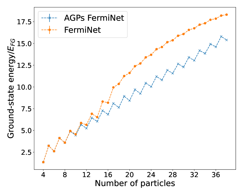
(a) The total energy of the UFG simulation cell, measured in units of the free Fermi gas energy $E_{\text{FG}}$. The original FermiNet Ansatz begins to fail when $N\gtrapprox 10$.

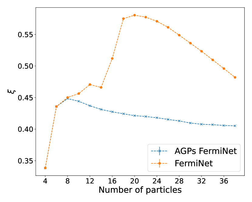
(b) The Bertsch parameter $\xi$ (the ratio of the interacting and non-interacting ground-state energies per particle) as a function of the number of particles $N$.

Figure 1: Comparison between results obtained using the AGPs FermiNet and the original FermiNet for different numbers of particles, $N$, with $r_{s}=1$ and $\mu=12$. All simulations used 32 determinants, 300,000 optimization steps, and the same hyperparameters, which are detailed in the Appendix.

We next compare our results with state-of-the-art FN-DMC results from Forbes et al. [21] shown in Fig. 2 for the case $k_{F}=1$ and $\mu=12$.

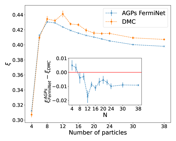
Figure 2: Comparison of the system-size dependent values of the Bertsch parameter, $\xi$, as calculated using the AGPs FermiNet and FN-DMC, with $k_{F}=1$ and $\mu=12$. According to the variational principle, lower values are better. The error bars on the AGPs FermiNet results are smaller than the sizes of the crosses. Inset: difference between the AGPs and FN-DMC values of the Bertsch parameter.

The AGPs FermiNet achieves a lower energy per particle than FN-DMC for all system sizes except for $N=4$ and $N=6$. The dependence of the Bertsch parameter on system size is also smoother when calculated with the AGPs FermiNet.

The pairing gap may be found using the approximation formula [56, 15]

$$\Delta=(-1)^{N}\left[E(N+1)-\frac{1}{2}\left[E(N)+E(N+2)\right]\right],$$ (38)

where $N$ is the total number of particles in the box. The results from $N=4$ to $N=36$ are shown in Fig. 3. Also shown is the thermodynamic ($N\rightarrow\infty$) limit of the BCS pairing gap including Gorkov’s polarization correction [57]:

$$\Delta_{\text{BCS}} =\frac{8}{e^{2}}\frac{\hbar^{2}k_{F}^{2}}{2m}\exp(\frac{\pi}{2k_{F}a}),$$ (39)

$$\Delta_{\text{Gorkov}} =\frac{1}{(4e)^{1/3}}\Delta_{\text{BCS}}.$$ (40)

Here $a$ is the scattering length of the interaction, which is infinite in the UFG. In this limit, $\Delta_{\text{BCS}}=1.804E_{\text{FG}}$ and $\Delta_{\text{Gorkov}}=0.815E_{\text{FG}}$, where $E_{\text{FG}}=\frac{3}{5}\frac{\hbar^{2}k_{F}^{2}}{2m}$ is the average energy per particle of an unpolarized non-interacting Fermi gas and $e$ is Euler’s number. The UFG is a strongly coupled system, so the BCS and Gorkov estimates of the gap need not be accurate.

The striking collapse of the pairing gap with increasing system size shows that the original FermiNet Ansatz struggles to describe paired states in systems of more than $10$ particles. The AGPs FermiNet Ansatz behaves much better, although the oscillations with system size suggest that significant finite-size errors remain even for the largest systems simulated.

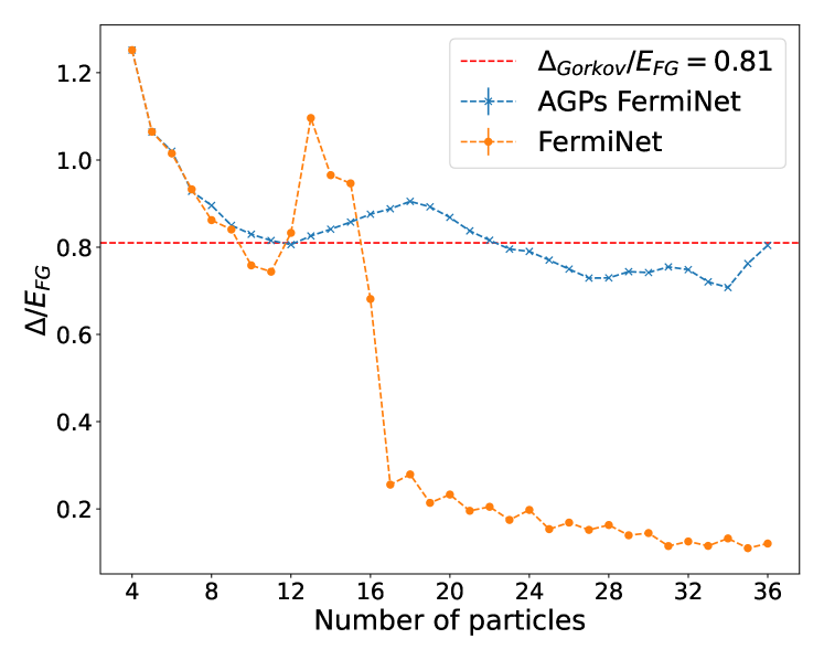
Figure 3: Pairing gaps calculated with the original FermiNet and the AGPs FermiNet for different numbers of particles $N$, with $r_{s}=1$ and $\mu=12$.

Another signature of fermionic superfluidity is the presence of off-diagonal long-ranged order in the two-body density matrix (TBDM),

$$\rho_{\uparrow\downarrow}^{(2)}(\mathbf{r}_{1},\mathbf{r}_{2};\mathbf{r}^{\prime}_{1},\mathbf{r}^{\prime}_{2})=\langle\hat{\psi}^{\dagger}_{\uparrow}(\mathbf{r}_{1})\hat{\psi}^{\dagger}_{\downarrow}(\mathbf{r}_{2})\hat{\psi}^{\phantom{\dagger}}_{\downarrow}(\mathbf{r}^{\prime}_{2})\hat{\psi}^{\phantom{\dagger}}_{\uparrow}(\mathbf{r}_{1}^{\prime})\rangle,$$ (41)

the largest eigenvalue of which diverges as the number of particles $N$ tends to infinity [58]. The superfluid condensate fraction $c$ may be obtained by evaluating [59]

$$c=\lim_{r\rightarrow\infty}\frac{\Omega^{2}}{N_{\uparrow}}\rho_{\uparrow\downarrow}^{(2)TR}(r),$$ (42)

where $\Omega$ is the volume of the simulation cell, $N_{\uparrow}$ is the number of spin-up particles, and $\rho_{\uparrow\downarrow}^{(2)TR}(r)$ is the rotational and translational average of the TBDM

$$\rho_{\uparrow\downarrow}^{(2)TR}(r)\\ =\frac{1}{4\pi r^{2}\Omega^{2}}\int\rho_{\uparrow\downarrow}^{(2)}(\mathbf{r}_{1},\mathbf{r}_{2};\mathbf{r}_{1}+\mathbf{r}^{\prime},\mathbf{r}_{2}+\mathbf{r}^{\prime})\delta(|\mathbf{r}^{\prime}|-r)d\mathbf{r}_{1}d\mathbf{r}_{2}d\mathbf{r}^{\prime}.$$ (43)

The one-body density matrix (OBDM), by contrast, tends to zero in the $r\rightarrow\infty$ limit [58]. A full discussion of the methods used to evaluate the condensate fraction in QMC simulations can be found in the Appendix and the CASINO manual [59].

After fully training both the original FermiNet and the AGPs FermiNet for the $N=38$ particle system, we used the resulting neural wave functions to compute the quantity $\frac{\Omega^{2}}{N_{\uparrow}}\rho_{\uparrow\downarrow}^{(2)TR}(r)$. The results are shown in Fig. 4, which provide further evidence that the original FermiNet fails to converge to the superfluid ground state; the quantity $\frac{\Omega^{2}}{N_{\uparrow}}\rho_{\uparrow\downarrow}^{(2)TR}(r)$ appears to be approaching zero in the large pair-separation limit, implying that the condensate fraction is also zero. The same quantity for the AGPs FermiNet approaches a finite value which we esitmated to be roughly $c=0.44(1)$ using the eight data points with separations $r/r_{s}\geq 2.0$. This value is consistent with previous estimations from experiments and the most recent AFMC value from [22]. Some of the results are summerized in Table (1)

Method	Value
Our estimation	0.44(1)
FN-DMC [60]	0.57(2)
FN-DMC and VMC with extrapolation [18]	0.51
FN-DMC with effective range extrapolation [61]	0.56(1)
AFMC [22]	0.43(2)
Experiment [62]	0.46(7)
Experiment [63]	0.47(7)

Table 1: The estimations of the superfluid condensate fraction at unitarity using various methods.

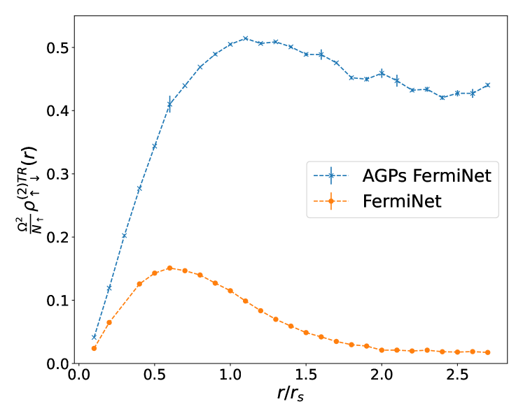
Figure 4: Comparing the TBDM estimators between the AGPs FermiNet and the original FermiNet with $N=38$, $r_{s}=1$ and $\mu=12$.

An important advantage of VMC methods is that almost any expectation value, including any reduced density matrix, may be estimated without bias. The same is not true of FN-DMC simulations, which sample the wave function instead of its square modulus and produce biased “one-sided” estimates of the expectation values of operators that do not commute with the Hamiltonian [14]. Thus, there are very few unbiased and accurate first-principles calculations of the condensate fraction. Our approach provides a solution to this problem and a more accurate way to estimate general expectation values.

VI Discussion

In this work, we studied the benchmark superfluid system of the UFG with neural wave functions . We showed that the original FermiNet Ansatz has difficulties in describing such a paired systems with strong and short-range attractive interactions between opposite spin particles. Hence, we proposed a way to improve the variational Ansatz by using determinants of FermiNet geminals, similar to an AGPs or a BCS wave function. We showed mathematically that the original FermiNet is a limiting case of the AGPs FermiNet despite the use of fewer parameters in the latter, which means that any FermiNet wave function can in-principle be written as an AGPs FermiNet wave function.

We compared the total energies and the energies per particle of the UFG between the original FermiNet and the AGPs FermiNet. The former fails to produce a paired state when the number of particles, $N$, is greater than around $10$, while the AGPs FermiNet works very well.

As the UFG has a superfluid ground-state, we computed the pairing gap and condensate fraction for the $N=38$ system and compared estimates made with the original FermiNet and the AGPs FermiNet. There is a clear qualitative difference between the pairing gap obtained using the AGPs FermiNet and the original FermiNet, with the latter approaching zero as the number of particle $N$ increases. The results for the superfluid condensate fraction show a similar behaviour, with the AGPs FermiNet converging to a finite value, while the original FermiNet approaches zero in the limit of large system size. Although the AGPs pairing gap shows significant finite size errors, it lies close to the mean-field BCS result with Gorkov-Melik-Barkhudarov corrections [57]. Taken together, these results show that the original FermiNet is unable to represent large systems with superfluid ground states. The AGPs FermiNet is much more suitable for studying paired systems such as the UFG.

To demonstrate success of the AGPs FermiNet, we also compared our calculated total energies with state-of-the-art fixed-node diffusion QMC energies obtained using a Jastrow-BCS Ansatz [21]. For all systems with more than a few particles, the AGPs FermiNet achieves lower (i.e., better) variational energies than FN-DMC using the same model interaction and system parameters.

The failure of the original FermiNet Ansatz comes as a surprise because the original FermiNet paper [1] argued that any many-body fermionic wave function can be represented as a single determinant of FermiNet orbitals. However, the mathematical argument relies on the construction of FermiNet orbitals with unphysical discontinuities. Whether or not any wave function can be represented as a single determinant of FermiNet orbitals of the type used in practice, which are differentiable everywhere except at electron-electron and electron-nuclear coalescence points, remains an open question. Another limitation is that the original FermiNet architecture, which is rather simple, may not be able to represent an arbitrary FermiNet orbital.

Even if a single FermiNet determinant is general in principle, there is no guarantee that it is equally easy to represent all wave functions. It may be that producing an accurate representation of a paired wave function requires the width and number of layers in the network to increase rapidly with system size. The observation that the original FermiNet works well when $N\lessapprox 10$ but that the quality of the results degrades rapidly for larger systems suggests that this is, in fact, the case.

One of the most important strengths of the original FermiNet is that it does not require the use of an explicit basis set. In particular, there is no need to construct and optimize a new basis set for every new system or particle. Our modified AGPs FermiNet for paired superfluids inherits this advantage.

Another strength of the AGPs FermiNet is the ease with which it is possible to optimize linear combinations of determinants of FermiNet pairing orbitals, such as the one in Eq. (35). This is much more difficult to accomplish with conventional wave functions based on explicit two-electron pairing orbitals or pairing orbitals represented as outer products of single-particle orbitals or basis functions. The basis-set-free nature of the AGPs FermiNet will make it relatively easy to investigate the importance of pairing in other systems of interest such as molecules, electron-positron systems, electron-hole liquids, and other $s$-wave superfluids.

The AGPs FermiNet introduced here is very general and flexible. It can be generalized to arbitrary pairing also with triplet spin components. Therefore, we expect it to become a powerfull tool for understanding strongly correlated non-$s$-wave superfluid and superconducting systems as well, for example Helium-3 or high-$T_{c}$ and $p$-wave superconductors.

Besides the FermiNet, future work may involve utilizing more recent neural-network architectures, such as the Psiformer [65], GLOBE and MOON [66], DeepErwin [67], etc., to build neural-network-based AGPs or Pfaffian wave functions.

Appendix A Antisymmetric Geminal Power Wave Function

This section discusses the relation between the antisymmetric geminal power singlet wave function (AGPs) and the BCS wave function.

A.1 Fixed-particle Number BCS Ground State

The antisymmetrized geminal power single (AGPs) wave function may be obtained by projecting the BCS ground-state wave function [13] into a subspace of fixed particle number [39]. We start with the BCS ground state:

$$\ket{\Psi_{\text{BCS}}} =\prod_{\mathbf{k}}(u_{\mathbf{k}}^{\phantom{\dagger}}+v_{\mathbf{k}}^{\phantom{\dagger}}\hat{c}^{\dagger}_{\mathbf{k},\uparrow}\hat{c}^{\dagger}_{-\mathbf{k},\downarrow})\ket{0}$$

$$=\bigg{(}\prod_{\mathbf{k}}u_{\mathbf{k}}^{\phantom{\dagger}}\bigg{)}e^{\sum_{\mathbf{k}}\varphi_{\mathbf{k}}^{\phantom{\dagger}}\hat{c}^{\dagger}_{\mathbf{k},\uparrow}\hat{c}^{\dagger}_{-\mathbf{k},\downarrow}}\ket{0},$$

where $\varphi_{\mathbf{k}}=\frac{v_{\mathbf{k}}}{u_{\mathbf{k}}}$. Ignoring global phase factors and coefficients, the fixed-particle BCS wave function can be written as:

$$\ket{\Psi_{\text{PBCS}}}=\bigg{(}\sum_{\mathbf{k}}\varphi_{\mathbf{k}}^{\phantom{\dagger}}\hat{c}^{\dagger}_{\mathbf{k},\uparrow}\hat{c}^{\dagger}_{-\mathbf{k},\downarrow}\bigg{)}^{p}\ket{0},$$ (44)

where $p=N/2$ is the number of pairs in the system and $N$ is the number of electrons. After Fourier transforming this wave function, we get the real space wave function [39]:

$$\Psi_{\text{PBCS}}=\mathcal{A}[\Phi(1,1^{\prime})\Phi(2,2^{\prime})\cdots\Phi(p,p^{\prime})],$$ (45)

where $\mathcal{A}$ is the antisymmetrizer, the wave function corresponding to $\Phi(i,i^{\prime})$ is

$$\Phi(i,i^{\prime}) \equiv\Phi(\mathbf{r}_{i},\sigma_{i};\mathbf{r}_{i^{\prime}}\sigma_{i^{\prime}})$$

$$=\varphi(\mathbf{r}_{i},\mathbf{r}_{i^{\prime}})\times\bra{\sigma_{i}\sigma_{i^{\prime}}}\frac{1}{\sqrt{2}}(\ket{\uparrow\downarrow}-\ket{\downarrow\uparrow}),$$ (46)

and $\varphi(\mathbf{r}_{i},\mathbf{r}_{i^{\prime}})=\sum_{\mathbf{k}}\varphi_{\mathbf{k}}e^{i\mathbf{k}\cdot(\mathbf{r}_{i}-\mathbf{r}_{i^{\prime}})}$ is the Fourier transform of $\varphi_{\mathbf{k}}$.

As mentioned in the main text, Eq. (45) can be written as a determinant of the pairing function $\varphi(\mathbf{r}_{i},\mathbf{r}_{i^{\prime}})$ after spin-assignment [39, 40]

$$\Psi_{\text{PBCS}}=\det\left[\varphi(\mathbf{r}^{\uparrow}_{i},\mathbf{r}^{\downarrow}_{j})\right].$$ (47)

Appendix B Experimental Setup

In this section, we report the FermiNet setup and hyperparameters used in this work.

B.1 FermiNet

The periodic version of the FermiNet implemented by Cassella et al. [38], which can be found in the FermiNet repository [69], was used as the basis for the AGPs code. The small modifications required to support AGPs wave functions were made using the JAX Python library [46]. For the majority of our calculations, four NVIDIA A100 GPUs were used. For systems with $N>30$ particles, we used four nodes with a total of sixteen A100 GPUs to speed up the calculations. A JAX implementation of the Kronecker-factored approximate curvature (KFAC) gradient descent algorithm [45, 70] was used for optimization. The FermiNet hyperparameters are shown in Table (2) and the network sizes in Table (3). All training runs used $3\times 10^{5}$ iterations to ensure convergence. When evaluating expectation values with an optimized wave function, $5\times 10^{4}$ inference steps were used.

Parameter	Value
Batch size	4096
Training iterations	3e5
Pretraining iterations	None
Learning rate	$(2e4+t)^{-1}$
Local energy clipping	5.0
KFAC Momentum	0
KFAC Covariance moving average decay	0.95
KFAC Norm constraint	1e-3
KFAC Damping	1e-3
MCMC Proposal std. dev. (per dimension)	0.02
MCMC Steps between parameter updates	10

Table 2: Hyperparameters used in all simulations.

Parameter	Value
One-electron Stream Network Size	512
Two-electron Stream Network Size	64
Number of Network Layers	4
Number of Determinants	32

Table 3: Network sizes and number of determinants used in all simulations.

B.2 Estimation of the Two-Body Density Matrix

The two-body density matrix (TBDM) in first quantized notation can be written as

$$\rho_{\alpha\beta}^{(2)}(\mathbf{r}_{1},\mathbf{r}_{2};\mathbf{r}^{\prime}_{1},\mathbf{r}^{\prime}_{2})\\ =N_{\alpha}(N_{\beta}-\delta_{\alpha\beta})\frac{\int|\Psi(\mathbf{R})|^{2}\frac{\Psi(\mathbf{r}^{\prime}_{1},\mathbf{r}^{\prime}_{2})}{\Psi(\mathbf{r}_{1},\mathbf{r}_{2})}d\mathbf{r}_{3}\dots d\mathbf{r}_{N}}{\int|\Psi(\mathbf{R})|^{2}d\mathbf{R}},$$ (48)

where $\alpha$ and $\beta$ denote the spin or particle species. The superfluid condensate fraction in a finite and periodic system is defined as

$$c=\frac{\Omega^{2}}{N_{\alpha}}\lim_{r\rightarrow\infty}\rho_{\alpha\beta}^{(2)TR}(r),$$ (49)

where $\Omega$ is the volume of the simulation cell, $N_{\alpha}$ is the number of particles with spin $\alpha$, and $\rho_{\alpha\beta}^{(2)TR}(r)$ is the translational and rotational average of the TBDM given in Eq. (43).

The one-body density matrix (OBDM) is expected to tend to zero as $r\rightarrow\infty$. However, because of finite-size effects, the OBDM is not necessarily zero within our simulation cell. We therefore use an improved estimator in Eq. (50) that removes the one-body contribution explicitly [59]:

$$\rho_{\alpha\beta}^{(2)}(\mathbf{r}_{1},\mathbf{r}_{2};\mathbf{r}^{\prime}_{1},\mathbf{r}^{\prime}_{2})=N_{\alpha}(N_{\beta}-\delta_{\alpha\beta})\frac{\int|\Psi(\mathbf{R})|^{2}\left[\frac{\Psi(\mathbf{r}^{\prime}_{1},\mathbf{r}^{\prime}_{2})}{\Psi(\mathbf{r}_{1},\mathbf{r}_{1})}-\frac{\Psi(\mathbf{r}^{\prime}_{1},\mathbf{r}_{2})}{\Psi(\mathbf{r}_{1},\mathbf{r}_{2})}\frac{\Psi(\mathbf{r}_{1},\mathbf{r}^{\prime}_{2})}{\Psi(\mathbf{r}_{1},\mathbf{r}_{2})}\right]d\mathbf{r}_{3}\dots d\mathbf{r}_{N}}{\int|\Psi(\mathbf{R})|^{2}d\mathbf{R}}.$$ (50)

This quantity can then be estimated using Monte Carlo sampling.

References

- Pfau et al. [2020] D. Pfau, J. S. Spencer, A. G. D. G. Matthews, and W. M. C. Foulkes, Phys. Rev. Res. 2, 033429 (2020).
- Leggett [1980] A. J. Leggett, in Modern Trends in the Theory of Condensed Matter, edited by A. Pekalski and J. A. Przystawa (Springer Berlin Heidelberg, Berlin, Heidelberg, 1980) pp. 13–27.
- Nozières and Schmitt-Rink [1985] P. Nozières and S. Schmitt-Rink, J. Low Temp. Phys. 59, 195 (1985).
- Papenbrock and Bertsch [1999] T. Papenbrock and G. F. Bertsch, Phys. Rev. C 59, 2052 (1999).
- Gandolfi et al. [2015] S. Gandolfi, A. Gezerlis, and J. Carlson, Annu. Rev. Nucl. Part. Sci. 65, 303 (2015), https://doi.org/10.1146/annurev-nucl-102014-021957 .
- Nishida and Son [2006] Y. Nishida and D. T. Son, Phys. Rev. Lett. 97, 050403 (2006).
- Nikolić and Sachdev [2007] P. Nikolić and S. Sachdev, Phys. Rev. A 75, 033608 (2007).
- Randeria et al. [1990] M. Randeria, J.-M. Duan, and L.-Y. Shieh, Phys. Rev. B 41, 327 (1990).
- Randeria [2010] M. Randeria, Nat. Phys. 6, 561 (2010).
- Strinati et al. [2018] G. C. Strinati, P. Pieri, G. Röpke, P. Schuck, and M. Urban, Phys. Rep. 738, 1 (2018), the BCS–BEC crossover: From ultra-cold Fermi gases to nuclear systems.
- Giorgini et al. [2008] S. Giorgini, L. P. Pitaevskii, and S. Stringari, Rev. Mod. Phys. 80, 1215 (2008).
- Chin et al. [2010] C. Chin, R. Grimm, P. Julienne, and E. Tiesinga, Rev. Mod. Phys. 82, 1225 (2010).
- Bardeen et al. [1957] J. Bardeen, L. N. Cooper, and J. R. Schrieffer, Phys. Rev. 106, 162 (1957).
- Foulkes et al. [2001] W. M. C. Foulkes, L. Mitas, R. J. Needs, and G. Rajagopal, Rev. Mod. Phys. 73, 33 (2001).
- Carlson et al. [2013] J. Carlson, S. Gandolfi, and A. Gezerlis, in Fifty Years of Nuclear BCS (WORLD SCIENTIFIC, 2013) pp. 348–359.
- Carlson et al. [2003] J. Carlson, S.-Y. Chang, V. R. Pandharipande, and K. E. Schmidt, Phys. Rev. Lett. 91, 050401 (2003).
- Chang et al. [2004] S. Y. Chang, V. R. Pandharipande, J. Carlson, and K. E. Schmidt, Phys. Rev. A 70, 043602 (2004), publisher: American Physical Society.
- Morris et al. [2010] A. J. Morris, P. López Ríos, and R. J. Needs, Phys. Rev. A 81, 033619 (2010).
- Chang and Pandharipande [2005] S. Y. Chang and V. R. Pandharipande, Phys. Rev. Lett. 95, 080402 (2005).
- Gezerlis and Carlson [2010] A. Gezerlis and J. Carlson, Phys. Rev. C 81, 025803 (2010).
- Forbes et al. [2011] M. M. Forbes, S. Gandolfi, and A. Gezerlis, Phys. Rev. Lett. 106, 235303 (2011).
- He et al. [2020] R. He, N. Li, B.-N. Lu, and D. Lee, Phys. Rev. A 101, 063615 (2020).
- Song et al. [2021] Y.-H. Song, Y. Kim, N. Li, B.-N. Lu, R. He, and D. Lee, Phys. Rev. C 104, 044304 (2021).
- Goulko and Wingate [2016] O. Goulko and M. Wingate, Phys. Rev. A 93, 053604 (2016).
- Jensen et al. [2020] S. Jensen, C. N. Gilbreth, and Y. Alhassid, Phys. Rev. Lett. 125, 043402 (2020).
- Pisani et al. [2022] L. Pisani, P. Pieri, and G. C. Strinati, Phys. Rev. B 105, 054505 (2022).
- Carleo and Troyer [2017] G. Carleo and M. Troyer, Science 355, 602 (2017), https://www.science.org/doi/pdf/10.1126/science.aag2302 .
- Choo et al. [2019] K. Choo, T. Neupert, and G. Carleo, Phys. Rev. B 100, 125124 (2019).
- Hibat-Allah et al. [2020] M. Hibat-Allah, M. Ganahl, L. E. Hayward, R. G. Melko, and J. Carrasquilla, Phys. Rev. Res. 2, 023358 (2020).
- Luo and Clark [2019] D. Luo and B. K. Clark, Phys. Rev. Lett. 122, 226401 (2019).
- Hermann et al. [2020] J. Hermann, Z. Schätzle, and F. Noé, Nat. Chem. 12, 891 (2020).
- Gerard et al. [2022] L. Gerard, M. Scherbela, P. Marquetand, and P. Grohs, arXiv:2205.09438 [cs.LG] (2022).
- Pescia et al. [2022] G. Pescia, J. Han, A. Lovato, J. Lu, and G. Carleo, Phys. Rev. Res. 4, 023138 (2022).
- Li et al. [2022a] X. Li, C. Fan, W. Ren, and J. Chen, Phys. Rev. Res. 4, 013021 (2022a).
- Wilson et al. [2021] M. Wilson, N. Gao, F. Wudarski, E. Rieffel, and N. M. Tubman, arXiv:2103.12570 [physics.chem-ph] (2021).
- Spencer et al. [2020a] J. S. Spencer, D. Pfau, A. Botev, and W. M. C. Foulkes, arXiv:2011.07125 [physics.comp-ph] (2020a).
- Li et al. [2022b] X. Li, Z. Li, and J. Chen, Nat. Commun. 13, 7895 (2022b).
- Cassella et al. [2023] G. Cassella, H. Sutterud, S. Azadi, N. D. Drummond, D. Pfau, J. S. Spencer, and W. M. C. Foulkes, Phys. Rev. Lett. 130, 036401 (2023).
- Bouchaud et al. [1988] J. Bouchaud, A. Georges, and C. Lhuillier, J. Phys. France 49, 553 (1988).
- Casula and Sorella [2003] M. Casula and S. Sorella, J. Chem. Phys. 119, 6500 (2003), arXiv:cond-mat/0305169.
- Bajdich [2007] M. Bajdich, Generalized pairing wave functions and nodal properties for electronic structure quantum monte carlo (2007), arXiv:0712.3066 [cond-mat.other] .
- Genovese et al. [2020] C. Genovese, T. Shirakawa, K. Nakano, and S. Sorella, Journal of Chemical Theory and Computation 16, 6114 (2020), pMID: 32804497, https://doi.org/10.1021/acs.jctc.0c00165 .
- Toulouse and Umrigar [2007] J. Toulouse and C. J. Umrigar, J. Chem. Phys. 126, 084102 (2007), https://doi.org/10.1063/1.2437215 .
- Hornik et al. [1989] K. Hornik, M. Stinchcombe, and H. White, Neural Netw. 2, 359 (1989).
- Martens and Grosse [2015] J. Martens and R. Grosse, in Proceedings of the 32nd International Conference on Machine Learning, Vol. 37, edited by F. Bach and D. Blei (PMLR, Lille, France, 2015) pp. 2408–2417.
- Bradbury et al. [2018] J. Bradbury, R. Frostig, P. Hawkins, M. J. Johnson, C. Leary, D. Maclaurin, G. Necula, A. Paszke, J. VanderPlas, S. Wanderman-Milne, and Q. Zhang, JAX: composable transformations of Python+NumPy programs (2018).
- Wilson et al. [2022] M. Wilson, S. Moroni, M. Holzmann, N. Gao, F. Wudarski, T. Vegge, and A. Bhowmik, arXiv:2202.04622 [physics.chem-ph] (2022).
- Note [1] Although, in principle, the particle coordinates are not needed in a periodic system, we have observed that including them often improves convergence and allows the variational Ansatz to achieve a lower energy. Hence, we have included them in all of our calculations.
- Casula et al. [2004] M. Casula, C. Attaccalite, and S. Sorella, J. Chem. Phys. 121, 7110 (2004), https://doi.org/10.1063/1.1794632 .
- Marchi et al. [2009] M. Marchi, S. Azadi, M. Casula, and S. Sorella, J. Chem. Phys. 131, 154116 (2009).
- Bajdich et al. [2006] M. Bajdich, L. Mitas, G. Drobný, L. K. Wagner, and K. E. Schmidt, Phys. Rev. Lett. 96, 130201 (2006).
- Xie et al. [2022] H. Xie, Z.-H. Li, H. Wang, L. Zhang, and L. Wang, arXiv:2209.06095 [cond-mat.str-el] (2022).
- Note [2] Note that the idea of an AGPs/BCS FermiNet is very similar to the previous work by Luo and Clark [30], where they used the neural network backflow (NNB) wave function implemented on top of a Bogoliubov-de Gennes/BCS wave function to study lattice systems.
- Note [3] To get a rough estimate of the number of terms in the sum, we can take the number of hidden units in the one-electron stream to be and the number of pairs to be , this number is approximately .
- Note [4] Although the range of the potential is finite, which introduces a second length scale even at unitarity, most of the results in the literature have been obtained with the same value of . This allows us to compare our results with theirs. To obtain exact results, one has to study the limit as , but converging the simulations becomes more difficult as increases.
- Palkanoglou et al. [2020] G. Palkanoglou, F. K. Diakonos, and A. Gezerlis, Phys. Rev. C 102, 064324 (2020).
- Gorkov and Melik-Barkhudarov [1961] L. P. Gorkov and T. K. Melik-Barkhudarov, Sov. Phys. JETP 13 (1961).
- Yang [1962] C. N. Yang, Rev. Mod. Phys. 34, 694 (1962).
- Needs et al. [2020] R. J. Needs, M. D. Towler, N. D. Drummond, P. López Ríos, and J. R. Trail, Variational and diffusion quantum Monte Carlo calculations with the CASINO code (2020), https://doi.org/10.1063/1.5144288 .
- Astrakharchik et al. [2005] G. E. Astrakharchik, J. Boronat, J. Casulleras, and S. Giorgini, Phys. Rev. Lett. 95, 230405 (2005).
- Li et al. [2011] X. Li, J. c. v. Kolorenč, and L. Mitas, Phys. Rev. A 84, 023615 (2011).
- Zwierlein et al. [2005] M. W. Zwierlein, C. H. Schunck, C. A. Stan, S. M. F. Raupach, and W. Ketterle, Phys. Rev. Lett. 94, 180401 (2005).
- Kwon et al. [2020] W. J. Kwon, G. D. Pace, R. Panza, M. Inguscio, W. Zwerger, M. Zaccanti, F. Scazza, and G. Roati, Science 369, 84 (2020), https://www.science.org/doi/pdf/10.1126/science.aaz2463 .
- Note [5] Shortly after submitting this manuscript to the arXiv server, a closely related preprint on neural networks and the Fermi gas appeared [68], proposing a similar extension to continuous-space neural network ansatzes.
- von Glehn et al. [2023] I. von Glehn, J. S. Spencer, and D. Pfau, arXiv:2211.13672 [physics.chem-ph] (2023).
- Gao and Günnemann [2023] N. Gao and S. Günnemann, arXiv:2302.04168 [cs.LG] (2023).
- Scherbela et al. [2022] M. Scherbela, R. Reisenhofer, L. Gerard, P. Marquetand, and P. Grohs, Nature Computational Science 2, 331 (2022).
- Kim et al. [2023] J. Kim, G. Pescia, B. Fore, J. Nys, G. Carleo, S. Gandolfi, M. Hjorth-Jensen, and A. Lovato, arXiv:2305.08831 [cond-mat.quant-gas] (2023).
- Spencer et al. [2020b] J. S. Spencer, D. Pfau, and contributors, FermiNet, http://github.com/deepmind/ferminet (2020b).
- Botev and Martens [2022] A. Botev and J. Martens, KFAC-JAX, http://github.com/deepmind/kfac-jax (2022).